Australian Rainfall & Runoff Revision Projects PROJECT 6 Loss Models for Catchment Simulation – Rural Catchments STAGE 3 REPORT P6/S3/016B OCTOBER 2014

Welcome message from author
This document is posted to help you gain knowledge. Please leave a comment to let me know what you think about it! Share it to your friends and learn new things together.
Transcript
Australian Rainfall & Runoff
Revision Projects
PROJECT 6
Loss Models for Catchment Simulation – Rural Catchments
STAGE 3 REPORT
P6/S3/016B
OCTOBER 2014

Engineers Australia Engineering House 11 National Circuit Barton ACT 2600 Tel: (02) 6270 6528 Fax: (02) 6273 2358 Email:[email protected] Web: www.arr.org.au
AUSTRALIAN RAINFALL AND RUNOFF REVISION PROJECT 6: LOSS MODELS FOR CATCHMENT SIMULATION: PHASE 4 ANALYSIS OF RURAL CATCHMENTS
PHASE 4 ANALYSIS OF LOSS VALUES FOR RURAL CATCHMENTS ACROSS AUSTRALIA
OCTOBER, 2014
Project Project 6: Loss models for catchment simulation: Phase 4 Analysis of Rural Catchments
ARR Report Number P6/S3/016B
Date 23 October 2014
ISBN 978-085825-9775
Contractor Jacobs SKM
Contractor Reference Number
VW07245
Authors Peter Hill Zuzanna Graszkiewicz Melanie Taylor Dr Rory Nathan
Verified by
P6/S3/016B : 23 October 2014
This project was made possible by funding from the
and the associated project are the result of a significant amount of in kind hours provided by
Engineers Australia Members.
Loss models for catchment simulation: Phase 4 Analysis of Rural Catchments
ACKNOWLEDGEMENTS
This project was made possible by funding from the Australian Federal Government.
project are the result of a significant amount of in kind hours provided by
ia Members.
Contractor Details
Jacobs SKM PO Box 312 Flinders Lane MELBOURNE VIC 8009
Tel: (03) 8668 3000 Fax: (03) 8668 3001
Web: www.JacobsSKM.com
Loss models for catchment simulation: Phase 4 Analysis of Rural Catchments
i
Federal Government. This report
project are the result of a significant amount of in kind hours provided by
Loss models for catchment simulation: Phase 4 Analysis of Rural Catchments
P6/S3/016B : 23 October 2014 ii
FOREWORD
ARR Revision Process
Since its first publication in 1958, Australian Rainfall and Runoff (ARR) has remained one of the
most influential and widely used guidelines published by Engineers Australia (EA). The current
edition, published in 1987, retained the same level of national and international acclaim as its
predecessors.
With nationwide applicability, balancing the varied climates of Australia, the information and the
approaches presented in Australian Rainfall and Runoff are essential for policy decisions and
projects involving:
• infrastructure such as roads, rail, airports, bridges, dams, stormwater and sewer
systems;
• town planning;
• mining;
• developing flood management plans for urban and rural communities;
• flood warnings and flood emergency management;
• operation of regulated river systems; and
• prediction of extreme flood levels.
However, many of the practices recommended in the 1987 edition of ARR now are becoming
outdated, and no longer represent the accepted views of professionals, both in terms of
technique and approach to water management. This fact, coupled with greater understanding of
climate and climatic influences makes the securing of current and complete rainfall and
streamflow data and expansion of focus from flood events to the full spectrum of flows and
rainfall events, crucial to maintaining an adequate knowledge of the processes that govern
Australian rainfall and streamflow in the broadest sense, allowing better management, policy
and planning decisions to be made.
One of the major responsibilities of the National Committee on Water Engineering of Engineers
Australia is the periodic revision of ARR. A recent and significant development has been that
the revision of ARR has been identified as a priority in the Council of Australian Governments
endorsed National Adaptation Framework for Climate Change.
The update will be completed in three stages. Twenty one revision projects have been identified
and will be undertaken with the aim of filling knowledge gaps. Of these 21 projects, ten projects
commenced in Stage 1 and an additional 9 projects commenced in Stage 2. The remaining
projects will commence in Stage 3. The outcomes of the projects will assist the ARR Editorial
Team with the compiling and writing of chapters in the revised ARR.
Steering and Technical Committees have been established to assist the ARR Editorial Team in
guiding the projects to achieve desired outcomes. Funding for Stages 1 and 2 of the ARR
revision projects has been provided by the Federal Department of Climate Change and Energy
Efficiency. Funding for Stages 2 and 3 of Project 1 (Development of Intensity-Frequency-
Duration information across Australia) has been provided by the Bureau of Meteorology.
Funding for Stage 3 has been provided by Geoscience Australia

Loss models for catchment simulation: Phase 4 Analysis of Rural Catchments
P6/S3/016B : 23 October 2014 iii
Project 6: Loss Models for Catchment Simulation
This project aims to develop design losses for the whole of Australia on rural and urban
catchments.
Mark Babister Assoc Prof James Ball
Chair Technical Committee for ARR Editor
ARR Research Projects

Loss models for catchment simulation: Phase 4 Analysis of Rural Catchments
P6/S3/016B : 23 October 2014 iv
ARR REVISION PROJECTS
The 21 ARR revision projects are listed below :
ARR Project No. Project Title Starting Stage
1 Development of intensity-frequency-duration information across Australia 1
2 Spatial patterns of rainfall 2
3 Temporal pattern of rainfall 2
4 Continuous rainfall sequences at a point 1
5 Regional flood methods 1
6 Loss models for catchment simulation 2
7 Baseflow for catchment simulation 1
8 Use of continuous simulation for design flow determination 2
9 Urban drainage system hydraulics 1
10 Appropriate safety criteria for people 1
11 Blockage of hydraulic structures 1
12 Selection of an approach 2
13 Rational Method developments 1
14 Large to extreme floods in urban areas 3
15 Two-dimensional (2D) modelling in urban areas. 1
16 Storm patterns for use in design events 2
17 Channel loss models 2
18 Interaction of coastal processes and severe weather events 1
19 Selection of climate change boundary conditions 3
20 Risk assessment and design life 2
21 IT Delivery and Communication Strategies 2

Loss models for catchment simulation: Phase 4 Analysis of Rural Catchments
P6/S3/016B : 23 October 2014 v
PROJECT TEAM
Project Team Members: � Dr Rory Nathan (AR&R TC and Jacobs SKM)
� Peter Hill (Jacobs SKM)
� Zuzanna Graszkiewicz (Jacobs SKM)
� Matthew Scorah (Jacobs SKM)
� David Stephens (Jacobs SKM)
� Clayton Johnson (Jacobs SKM)
� Stephen Impey (Jacobs SKM)
� Dr Ataur Rahman (EnviroWater Sydney)
� Melanie Loveridge (EnviroWater Sydney)
� Leanne Pearce (WA Water Corporation)
This report was independently reviewed by:
• Erwin Weinmann

Loss models for catchment simulation: Phase 4 Analysis of Rural Catchments
P6/S3/016B : 23 October 2014 vi
BACKGROUND
ARR Project 6 - Loss models for catchment simulation - consists of four phases of
work as defined in the outcomes of the workshop of experts in the field held in 2009. These
are:
• Phase 1 – Pilot Study for Rural Catchments. A pilot study on a limited number of
catchments that trials potential loss models to test whether they are suited for
parameterisation and application to design flood estimation for ungauged catchments.
• Phase 2 – Collate Data for Rural Catchments. Streamflow and rainfall data for a large
number of catchments across Australia will be collated for subsequent analysis.
• Phase 3 – Urban Losses. The phase involves analysis of losses for urban areas and
estimation of impervious areas.
• Phase 4 – Analysis of Data for Catchments across Australia. Loss values will be
derived in a consistent manner from the analysis of recorded streamflow and
rainfall from catchments across Australia. The results will then be analysed to
determine the distribution of loss values, correlation between loss parameters and
variation with storm severity, duration and season. Finally, prediction equations will be
developed that relate the loss values to catchment characteristics.
This report details the outcomes of Phase 4.
Loss models for catchment simulation: Phase 4 Analysis of Rural Catchments
P6/S3/016B : 23 October 2014 vii
AR&R Technical Committee:
Chair: Mark Babister, WMAwater
Members: Associate Professor James Ball, Editor AR&R, UTS
Professor George Kuczera, University of Newcastle
Professor Martin Lambert, Chair NCWE, University of Adelaide
Dr Rory Nathan, Jacobs SKM
Dr Bill Weeks, Department of Transport and Main Roads, Qld
Associate Professor Ashish Sharma, UNSW
Dr Bryson Bates, CSIRO
Steve Finlay, Engineers Australia
Related Appointments:
ARR Project Engineer: Monique Retallick, WMAwater
Loss models for catchment simulation: Phase 4 Analysis of Rural Catchments
P6/S3/016B : 23 October 2014 viii
TABLE OF CONTENTS
1. Introduction ............................................................................................................... 1
2. Study catchments ..................................................................................................... 2
3. Selection of conceptual loss models ...................................................................... 6
3.1. Introduction ................................................................................................. 6
3.2. Initial Loss – Continuing Loss ..................................................................... 7
3.3. SWMOD ..................................................................................................... 8
3.3.1. Distributed storage capacity models ........................................................... 8
3.3.2. SWMOD overview ...................................................................................... 9
3.3.3. SWMOD conceptualisation ....................................................................... 10
3.4. Estimation of profile water holding capacity .............................................. 11
3.4.1. Introduction ............................................................................................... 11
3.4.2. Shape parameter ...................................................................................... 12
3.4.3. Comparison with other studies .................................................................. 13
4. Selection and characterisation of storm events ................................................... 15
4.1. Embedded nature of design rainfall bursts ................................................ 15
4.2. Selection and definition of storm events .................................................... 16
4.2.1. Selection of bursts .................................................................................... 16
4.2.2. Definition of complete storms .................................................................... 16
4.3. Pre-burst rainfall ....................................................................................... 17
4.4. Variation of pre-burst rainfall ..................................................................... 18
4.4.1. Pre-burst variation with design rainfall ...................................................... 18
4.4.2. Pre-burst variation with burst duration....................................................... 19
4.4.3. Pre-burst as a proportion of burst depth .................................................... 22
4.4.4. Pre-burst variation with burst severity ....................................................... 24
5. Estimation of loss values ....................................................................................... 25
5.1. Baseflow separation ................................................................................. 25
5.2. Method ..................................................................................................... 25
5.3. Review of loss values ............................................................................... 27
5.4. Routing parameters .................................................................................. 29
6. Loss values ............................................................................................................. 31
6.1. Storm loss values ..................................................................................... 31
Loss models for catchment simulation: Phase 4 Analysis of Rural Catchments
P6/S3/016B : 23 October 2014 ix
6.2. Relationship between Storm Initial Loss and Initial Moisture ..................... 34
6.3. Sensitivity to burst duration ....................................................................... 37
6.4. Burst loss values ...................................................................................... 38
6.5. Comparison with previous studies ............................................................ 39
6.5.1. Comparison with Pilot Study ..................................................................... 39
6.5.2. Comparison with other studies .................................................................. 40
6.6. Relative performance of loss models ........................................................ 41
6.7. Non-parametric distribution ....................................................................... 42
6.8. Relationship with antecedent conditions ................................................... 45
6.9. Variation with storm severity ..................................................................... 47
7. Development of prediction equations ................................................................... 49
7.1. Catchment characteristics ......................................................................... 49
7.2. Multiple linear regression approach .......................................................... 51
7.3. Selection of independent variables ........................................................... 52
7.4. Prediction equations ................................................................................. 53
7.4.1. GSAM Coastal and Inland Region ............................................................ 53
7.4.2. GTSMR Coastal ....................................................................................... 54
7.4.3. GTSMR SW WA ....................................................................................... 55
7.4.4. Range of applicability ................................................................................ 55
8. Conclusions and recommendations...................................................................... 56
9. References .............................................................................................................. 59
Appendix A Excluded catchments ............................................................................. 63
Appendix B Catchment maps ..................................................................................... 66
Appendix C Pre-burst distribution for each duration ............................................... 67
Appendix D Ratio of 3 hour to 6 hour pre-burst relationships ................................. 70
Appendix E Pre-burst distributions and API for each site and duration ................. 71
Appendix F Distribution of pre-burst rainfall for each region .................................. 72
Appendix G Sensitivity of loss values to approach .................................................. 73
Appendix H Adopted routing and baseflow parameters ........................................ 103
Appendix I Loss summaries for 24h bursts ........................................................... 104
Appendix J Loss summaries for 3h bursts ............................................................. 105
Appendix K Non-parametric loss distributions ....................................................... 106
Appendix L Variation of loss values with ARI ......................................................... 110
Appendix M Prediction equation diagnostics .......................................................... 119

Loss models for catchment simulation: Phase 4 Analysis of Rural Catchments
P6/S3/016B: 23 October 2014 1
1. Introduction
Engineers Australia has embarked upon the revision of Australian Rainfall and Runoff (ARR).
The revision is being undertaken over 4 years and is being underpinned by 21 projects which
address knowledge gaps or developments since the last full revision in 1987. ARR Project 6 -
Loss models for catchment simulation - consists of four phases of work:
� Phase 1 – Pilot Study for Rural Catchments (SKM, 2012b; Hill et al., 2011). Involved a pilot
study on a limited number of catchments that trialled potential loss models to test whether
they are suited for parameterisation and application to design flood estimation for ungauged
catchments.
� Phase 2 – Collation of Data for Rural Catchments (SKM, 2012a). Streamflow and rainfall
data for a large number of catchments across Australia was collated for subsequent
analysis.
� Phase 3 – Urban Losses. The phase involves analysis of losses for urban areas and
estimation of impervious areas.
� Phase 4 – Analysis of Loss Values for Rural Catchments across Australia. Loss values have
been derived in a consistent manner from the analysis of recorded streamflow and rainfall
from catchments across Australia and then analysed to determine the distribution of loss
values. Finally, prediction equations were developed that relate the loss values to catchment
characteristics.
This report covers the work undertaken as part of Phase 4. The following chapters of the report
are summarised below:
� Chapter 2 outlines the basis of selecting catchments and summarises the adopted
catchments for the study;
� Chapter 3 introduces and discusses the conceptual loss models applied which builds on the
outcomes of the Pilot Study undertaken as part of Phase 1.
� Chapter 4 describes the selection and characterisation of events analysed, with particular
emphasis on rainfall occurring immediately prior to these bursts of rainfall
� Chapter 5 describes the approach used to estimate the loss values.
� Chapter 6 presents the estimated loss values and explores relationships with antecedent
conditions and storm severity
� Chapter 7 explores the relationship between the loss values and catchment characteristics
and prediction equations for each of the loss parameters for different hydroclimatic regions
across Australia.
� Chapter 8 covers conclusions and recommendations from the study.
Loss models for catchment simulation: Phase 4 Analysis of Rural Catchments
P6/S3/016B: 23 October 2014 2
2. Study catchments
The estimation of loss values requires catchments with concurrent periods of pluviograph and
streamflow records. Sufficient rainfall stations are required to adequately capture the total
volume of rainfall. The catchment should be sufficiently small so that routing effects are not
significant and hence estimated loss values are not sensitive to the catchment routing
assumptions.
The greatest constraint on the selection of appropriate catchments for inclusion in the study was
found to be representative rainfall records for the catchments. There is hence an implicit trade-
off between analysing a greater number of catchments and the quality of the spatial coverage of
rainfall.
Phase 2 of ARR Project #6 involved the identification and collation of data sets for rural
catchments. The adopted criteria for selection of the catchments were:
� catchment area between 20 and 100 km2
� unregulated (free from transfers and lake systems)
� minimum of 20 years of streamflow record with a preference for a longer period
� close proximity of a pluviograph gauge to the catchment centroid, preferably within 5 km
� at least 20 years of overlapping streamflow and pluviograph data
� mix of catchments covering different regions of Australia
A preliminary list of compliant catchments based on catchment area and streamflow record was
made using the Bureau of Meteorology (BoM) Water Resource Station Catalogue (WRSC). This
database includes sites maintained by BoM and other agencies.
The catchments were initially defined using the national 9” (9 second) Digital Elevation Model
(DEM). This DEM covers the whole of Australia and has a grid spacing of 9 seconds in longitude
and latitude, which equates to approximately 250 metres. It has been “hydrologically enforced”
to consolidate and incorporate streamline flow paths and other topological features. The
hydrological enforcing used flow direction from the 9 second DEM and the gauge locations to
define a preliminary catchment boundary and area. An approximate catchment centroid location
was determined for each catchment and used to obtain the closest pluviograph stations to each
catchment based on the WRSC dataset.
The preliminary catchment boundaries were used to determine that the catchment fulfilled the
criteria listed above for being free of significant water bodies and not located in urban areas. The
period of hourly rainfall record at the pluviograph stations identified was compared to the period
of streamflow record. Where the period of concurrent streamflow and hourly rainfall was greater
than 20 years, the catchment was considered eligible for the Phase 2 database.
The streamflow and pluviograph data was collected from state agencies and the Bureau of
Meteorology. As part of Phase 2 preliminary data checks were done collected data, including
comparison of the mean annual rainfall calculated from the received data and the mean annual
rainfall determined from the BoM Average Annual Rainfall raster dataset. Mean annual
Loss models for catchment simulation: Phase 4 Analysis of Rural Catchments
P6/S3/016B: 23 October 2014 3
streamflow was also checked by plotting against mean annual rainfall for each site. These
checks were used to identify any gross errors in the data.
A number of catchments were then excluded from the analysis based on problems with the
collected data, including missing periods, shorter periods of record or timing issues. Some other
catchments were excluded because they occurred in areas of high density of eligible
catchments (for example SW WA). Of the available catchments in these areas, those with the
longest period of overlapping streamflow and pluviograph data and the closest distance between
the pluviograph and the catchment centroid were selected. Appendix A shows a list of
catchments that were initially identified as potentially fulfilling the criteria but subsequently
excluded, and the reason for the exclusion.
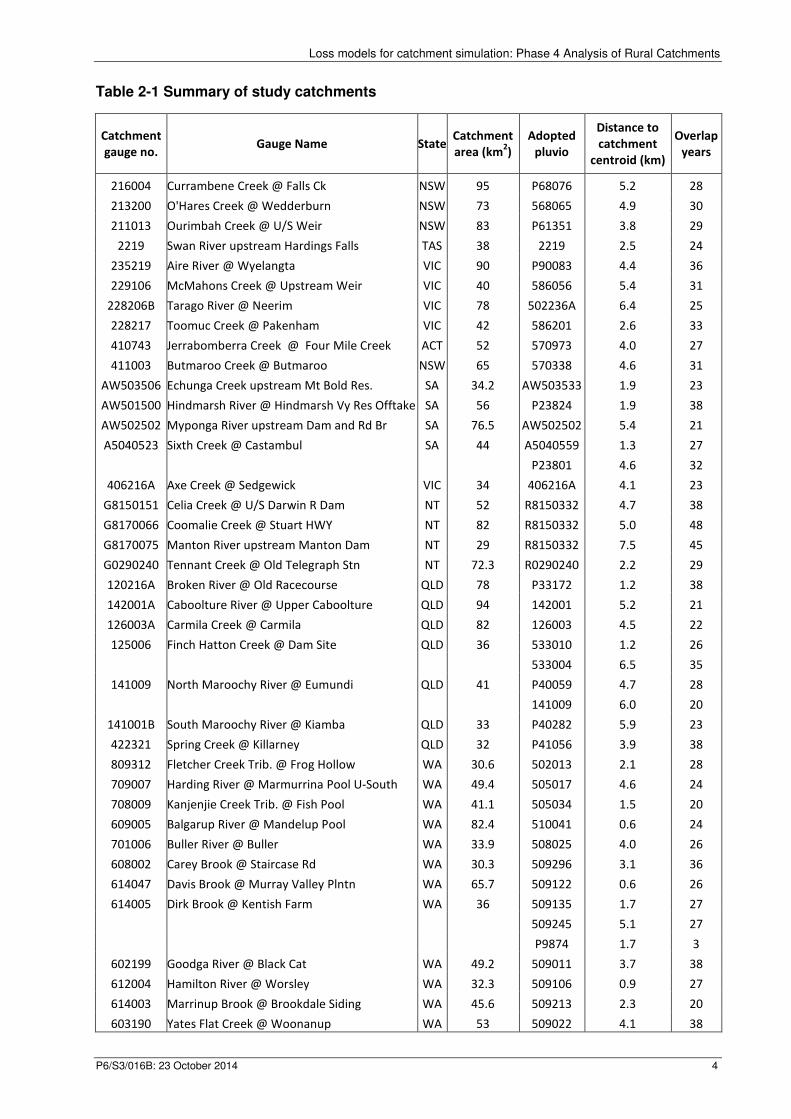
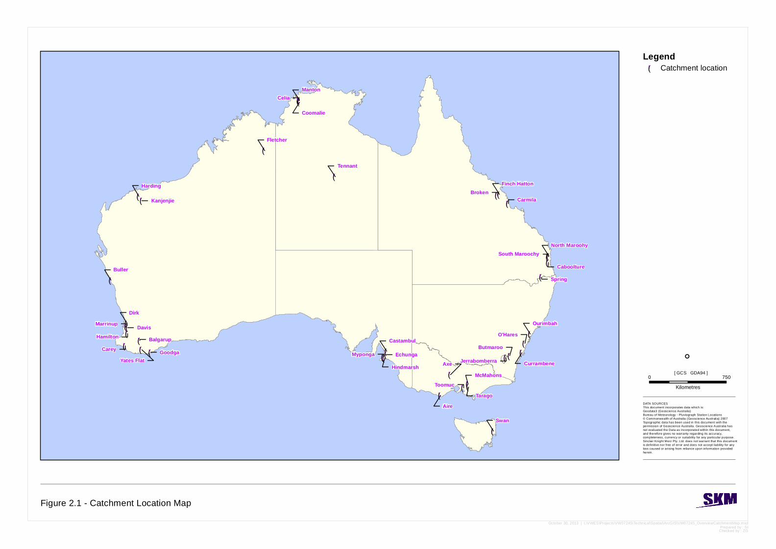
A total of 38 catchments were ultimately included in the Phase 4 analysis. Ten of these were the
pilot catchments from the Phase 1 Pilot Study. The final set of catchments is listed in Table 2-1
and shown in Figure 2-1. Maps of each catchment are included in Appendix B.
The investigation of the loss values described in Section 6 showed the influence of different
hydroclimatic regions across Australia. From preliminary analysis of the data, the regions
defined by the BoM in the development of the generalised PMP estimates were adopted as they
are based upon the prevalent storm types and appeared useful in explaining the variability of
loss values. These groups of catchments have been subsequently used in summarising the
results and developing prediction equations.
The GTSMR (Generalised Tropical Storm Method – Revised) region covers those areas of
Australia affected by storms of tropical origin. The storms within the GSTMR can be broadly
classified as tropical cyclones, ex-tropical cyclones, Monsoon activity and extratropical systems.
Each of these types of storms can be limited to certain areas and to certain times of the year.
Thus, the BoM has divided the GTSMR zone into sub-zones to represent the particular type of
storm mechanism that would be important (BoM, 2003). The regions are Coastal, Inland and
Southwest WA (although none of the Project 6 catchments lie in the GTSMR inland region)
The remainder of Australia is the defined as the GSAM (Generalised South eastern Australia
Method). The GSAM region has been divided into two zones, Coastal and Inland, separated by
the Great Dividing Range. This zonal division reflects a working hypothesis that within the two
zones the mechanisms by which large rainfalls are produced are genuinely different. The
corollary is that within each zone there is an assumed homogeneity (BoM, 1996).
Loss models for catchment simulation: Phase 4 Analysis of Rural Catchments
P6/S3/016B: 23 October 2014 4
Table 2-1 Summary of study catchments
Catchment
gauge no. Gauge Name State
Catchment
area (km2)
Adopted
pluvio
Distance to
catchment
centroid (km)
Overlap
years
216004 Currambene Creek @ Falls Ck NSW 95 P68076 5.2 28
213200 O'Hares Creek @ Wedderburn NSW 73 568065 4.9 30
211013 Ourimbah Creek @ U/S Weir NSW 83 P61351 3.8 29
2219 Swan River upstream Hardings Falls TAS 38 2219 2.5 24
235219 Aire River @ Wyelangta VIC 90 P90083 4.4 36
229106 McMahons Creek @ Upstream Weir VIC 40 586056 5.4 31
228206B Tarago River @ Neerim VIC 78 502236A 6.4 25
228217 Toomuc Creek @ Pakenham VIC 42 586201 2.6 33
410743 Jerrabomberra Creek @ Four Mile Creek ACT 52 570973 4.0 27
411003 Butmaroo Creek @ Butmaroo NSW 65 570338 4.6 31
AW503506 Echunga Creek upstream Mt Bold Res. SA 34.2 AW503533 1.9 23
AW501500 Hindmarsh River @ Hindmarsh Vy Res Offtake SA 56 P23824 1.9 38
AW502502 Myponga River upstream Dam and Rd Br SA 76.5 AW502502 5.4 21
A5040523 Sixth Creek @ Castambul SA 44 A5040559 1.3 27
P23801 4.6 32
406216A Axe Creek @ Sedgewick VIC 34 406216A 4.1 23
G8150151 Celia Creek @ U/S Darwin R Dam NT 52 R8150332 4.7 38
G8170066 Coomalie Creek @ Stuart HWY NT 82 R8150332 5.0 48
G8170075 Manton River upstream Manton Dam NT 29 R8150332 7.5 45
G0290240 Tennant Creek @ Old Telegraph Stn NT 72.3 R0290240 2.2 29
120216A Broken River @ Old Racecourse QLD 78 P33172 1.2 38
142001A Caboolture River @ Upper Caboolture QLD 94 142001 5.2 21
126003A Carmila Creek @ Carmila QLD 82 126003 4.5 22
125006 Finch Hatton Creek @ Dam Site QLD 36 533010 1.2 26
533004 6.5 35
141009 North Maroochy River @ Eumundi QLD 41 P40059 4.7 28
141009 6.0 20
141001B South Maroochy River @ Kiamba QLD 33 P40282 5.9 23
422321 Spring Creek @ Killarney QLD 32 P41056 3.9 38
809312 Fletcher Creek Trib. @ Frog Hollow WA 30.6 502013 2.1 28
709007 Harding River @ Marmurrina Pool U-South WA 49.4 505017 4.6 24
708009 Kanjenjie Creek Trib. @ Fish Pool WA 41.1 505034 1.5 20
609005 Balgarup River @ Mandelup Pool WA 82.4 510041 0.6 24
701006 Buller River @ Buller WA 33.9 508025 4.0 26
608002 Carey Brook @ Staircase Rd WA 30.3 509296 3.1 36
614047 Davis Brook @ Murray Valley Plntn WA 65.7 509122 0.6 26
614005 Dirk Brook @ Kentish Farm WA 36 509135 1.7 27
509245 5.1 27
P9874 1.7 3
602199 Goodga River @ Black Cat WA 49.2 509011 3.7 38
612004 Hamilton River @ Worsley WA 32.3 509106 0.9 27
614003 Marrinup Brook @ Brookdale Siding WA 45.6 509213 2.3 20
603190 Yates Flat Creek @ Woonanup WA 53 509022 4.1 38
!(!(!(
!(
!(
!(!(!(!( !(
!(!(!(
!(!(
!(!(!(!( !(
!( !(!(!( !(!( !(!( !(!( !(!(
!(
!(!(!(!(
!(
MantonCelia
Coomalie
Fletcher
Tennant
Finch HattonBroken
Harding
Kanjenjie Carmila
North MaroohySouth Maroochy
Caboolture
SpringBuller
DirkMarrinup DavisHamilton
Ourimbah
Balgarup O'Hares
CareyYates Flat
CastambulGoodga
CurrambeneEchunga
ButmarooMyponga
JerrabomberraHindmarsh Axe
McMahons
TaragoToomuc
Aire
Swan
[ GCS GDA94 ]°
0 750Kilometres
October 30, 2013 | I:\VWES\Projects\VW07245\Technical\Spatial\ArcGIS\VW07245_OverviewCatchmentMap.mxdPrepared by : SIChecked by : ZG
Legend!( Catchment location
DATA SOURCESThis document incorporates data which is:Geodata3 (Geoscience Australia)Bureau of Meteorology - Pluviograph Station Locations© Commonwealth of Australia (Geoscience Australia) 2007Topographic data has been used in this document with thepermission of Geoscience Australia. Geoscience Austral ia hasnot evaluated the Data as incorporated within this document,and therefore gives no warranty regarding its accuracy,completeness, currency or suitability for any particular purpose.Sinclair Knight Merz Pty. Ltd. does not warrant that this documentis definitive nor free of error and does not accept liability for anyloss caused or arising from reliance upon information providedherein.
Figure 2.1 - Catchment Location Map
Loss models for catchment simulation: Phase 4 Analysis of Rural Catchments
P6/S3/016B: 23 October 2014 6
3. Selection of conceptual loss models
3.1. Introduction
Loss is defined as the precipitation that does not appear as direct runoff, and the loss is typically
attributed to processes such as interception by vegetation, infiltration into the soil, retention on
the surface (depression storage), and transmission loss through the stream bed and banks.
While the processes that contribute to loss may be well defined at a point, it is difficult to
estimate a representative value of loss over an entire catchment. Other factors, such as the
spatial variability in topography, catchment characteristics (such as vegetation and soils), and
rainfall makes it very difficult to link the loss to catchment characteristics.
Despite the obvious attraction of using infiltration equations; the uncertainties of characterising
catchment properties (particularly soil) do not justify the use of anything more than the simplest
models (Mein and Goyen, 1988). To overcome this difficulty, lumped conceptual loss models are
widely used for design flood estimation. They combine the different loss processes and treat
them in a simplified fashion. The focus of these conceptual models is less on the representation
of the loss processes themselves, but is rather on representing their effects in producing the
rainfall excess.
The key requirements for a loss model for design flood estimation are to (Weinmann, pers.
Comm.):
� close the volume balance in a probabilistic sense such that the volume of the design flood
hydrograph for a given AEP should match the flood volume derived from the frequency
analysis of flood volumes;
� produce a realistic time distribution of runoff to allow the modelling of the peak flow and
hydrograph shape;
� reflect the variation of runoff production with different catchment characteristics to enable
application to ungauged catchments; and,
� reflect the effects of natural variability of runoff production for different events on the same
catchment to avoid probability bias in the transformation of rainfall to flood.
In the Phase 1 Pilot Study (Hill et al., 2013) a number of criteria were used to assess candidate
loss models; namely it was required that the model :
1) produces a temporal distribution of rainfall-excess that is consistent with the effect of the
processes contributing to loss
2) is suitable for extrapolation beyond calibration and hence applicable to estimate floods over
a full range of AEPs
3) has inputs that are consistent with data readily available across Australia
4) is parsimonious (i.e. preferably requires no more than two parameters to be fitted)
5) has parameters that have been linked to catchment characteristics, or it is considered
reasonable that such a link could be established
6) is readily accessible and well documented ; and,
7) can be easily incorporated into rainfall-runoff models
Loss models for catchment simulation: Phase 4 Analysis of Rural Catchments
P6/S3/016B: 23 October 2014 7
The four loss models selected for further consideration were:
1) Initial loss – constant continuing loss (IL/CL)
2) Initial loss – constant proportional loss (IL/PL)
3) Initial loss – variable continuing loss; and,
4) Probability distributed storage capacity loss model.
The IL/PL model provided satisfactory results when used to estimate loss values but when
combined with other design inputs there was a tendency to underestimate peak flows when
compared to those from the frequency analysis of recorded peak flows. This reinforces the
difficulties of applying the IL/PL model to derive design estimates beyond the range of events
found in the historical record.
Based upon consideration of infiltration theory it would be expected that the infiltration rate
should decrease with the volume of water infiltrated. For the IL/CL model this would suggest that
the Continuing Loss should decrease as the event progresses and such a reduction with
duration (as a surrogate for volume of infiltration) has been observed from the empirical analysis
of data by Ishak and Rahman (2006) and Ilahee and Imteaz (2009). The Phase 1 pilot study did
not identify a reduction in the continuing loss rate with duration or infiltrated volume.
Thus, it was recommended that Phase 4 concentrate on deriving parameter values for IL/CL and
SWMOD.
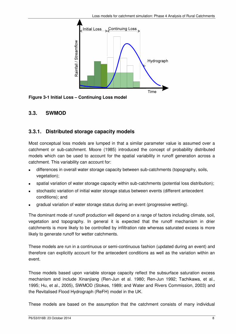
3.2. Initial Loss – Continuing Loss
The most commonly-used model in Australia is the Initial Loss - Continuing Loss (IL/CL) model
(Figure 3-1). The initial loss occurs in the beginning of the storm, prior to the commencement of
surface runoff. It should be noted that when analysing recorded streamflow data the start of the
hydrograph rise reflects the runoff response from the parts of the catchment closest to the
gauging station and the commencement of runoff from the upper parts of the catchments is not
readily discernible because of routing delays. This limitation is overcome if the initial loss is
inferred from a routing-routing model.
The continuing loss is the average rate of loss throughout the remainder of the storm. This
model is consistent with the concept of runoff being produced by infiltration excess, i.e. runoff
occurs when the rainfall intensity exceeds the infiltration capacity of the soil.
A number of models (such as URBS and HEC-HMS) include loss models that allow recovery of
the Initial Loss after a substantial dry period. The recovering loss model is represented as a
simple initial loss single bucket model. When rainfall is less than the potential loss in a time step,
the deficit is made up in part from the initial loss store. Although accounting for the recovery of
Initial Loss may be important for long duration events which have multiple bursts, it is unlikely to
be significant for design flood estimation which is based upon design bursts or design storms
where the rainfall is reasonably continuous over the event.
Loss models for catchment simulation: Phase 4 Analysis of Rural Catchments
P6/S3/016B: 23 October 2014 8
Figure 3-1 Initial Loss – Continuing Loss model
3.3. SWMOD
3.3.1. Distributed storage capacity models
Most conceptual loss models are lumped in that a similar parameter value is assumed over a
catchment or sub-catchment. Moore (1985) introduced the concept of probability distributed
models which can be used to account for the spatial variability in runoff generation across a
catchment. This variability can account for:
� differences in overall water storage capacity between sub-catchments (topography, soils,
vegetation);
� spatial variation of water storage capacity within sub-catchments (potential loss distribution);
� stochastic variation of initial water storage status between events (different antecedent
conditions); and
� gradual variation of water storage status during an event (progressive wetting).
The dominant mode of runoff production will depend on a range of factors including climate, soil,
vegetation and topography. In general it is expected that the runoff mechanism in drier
catchments is more likely to be controlled by infiltration rate whereas saturated excess is more
likely to generate runoff for wetter catchments.
These models are run in a continuous or semi-continuous fashion (updated during an event) and
therefore can explicitly account for the antecedent conditions as well as the variation within an
event.
Those models based upon variable storage capacity reflect the subsurface saturation excess
mechanism and include Xinanjiang (Ren-Jun et al. 1980; Ren-Jun 1992; Tachikawa, et al.,
1995; Hu, et al., 2005), SWMOD (Stokes, 1989; and Water and Rivers Commission, 2003) and
the Revitalised Flood Hydrograph (ReFH) model in the UK.
These models are based on the assumption that the catchment consists of many individual
P6/S3/016B: 23 October 2014
storage elements with a soil moisture capacity.
catchment is probabilistic, in other words the different amounts of soil mois
assigned to specific locations in the catchment.
by rainfall and decreased by evaporation. When rainfall exceeds the st
runoff is produced. The model assumes that th
elements between rainfall events.
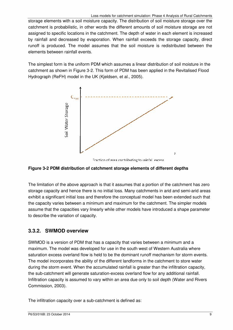
The simplest form is the uniform PDM
catchment as shown in Figure
Hydrograph (ReFH) model in the UK (Kjeldsen, et al., 2005).
Figure 3-2 PDM distribution of catchment storage elements o
The limitation of the above approach is that it assumes that a portion of the catchment has zero
storage capacity and hence there is no
exhibit a significant initial loss
the capacity varies between a minimum and maximum for the catchment. The simpler models
assume that the capacities vary linearly while other models have introduced a shape parameter
to describe the variation of capacity.
3.3.2. SWMOD overview
SWMOD is a version of PDM that has a capacity that varies between a minimum and a
maximum. The model was developed for use in the south west of Western Australia where
saturation excess overland flow is held to be the dominant runoff mechanism for s
The model incorporates the ability of the different landforms in the catchment to store water
during the storm event. When the accumulated rainfall is greater than the infiltration capacity,
the sub-catchment will generate saturation
Infiltration capacity is assumed to vary within an area due only to soil depth
Commission, 2003).
The infiltration capacity over a sub
Loss models for catchment simulation: Phase 4 Analysis of Rural Catchments
storage elements with a soil moisture capacity. The distribution of soil moisture storage over the
catchment is probabilistic, in other words the different amounts of soil mois
assigned to specific locations in the catchment. The depth of water in each element is increased
and decreased by evaporation. When rainfall exceeds the st
is produced. The model assumes that the soil moisture is redistributed between the
elements between rainfall events.
The simplest form is the uniform PDM which assumes a linear distribution of soil moisture in the
Figure 3-2. This form of PDM has been applied in the Revitalised Flood
drograph (ReFH) model in the UK (Kjeldsen, et al., 2005).
PDM distribution of catchment storage elements of different depths
tion of the above approach is that it assumes that a portion of the catchment has zero
storage capacity and hence there is no initial loss. Many catchments in arid and semi
oss and therefore the conceptual model has been extended such that
the capacity varies between a minimum and maximum for the catchment. The simpler models
assume that the capacities vary linearly while other models have introduced a shape parameter
to describe the variation of capacity.
erview
SWMOD is a version of PDM that has a capacity that varies between a minimum and a
maximum. The model was developed for use in the south west of Western Australia where
saturation excess overland flow is held to be the dominant runoff mechanism for s
The model incorporates the ability of the different landforms in the catchment to store water
during the storm event. When the accumulated rainfall is greater than the infiltration capacity,
catchment will generate saturation-excess overland flow for any additional rainfall.
Infiltration capacity is assumed to vary within an area due only to soil depth
The infiltration capacity over a sub-catchment is defined as:
Loss models for catchment simulation: Phase 4 Analysis of Rural Catchments
9
The distribution of soil moisture storage over the
catchment is probabilistic, in other words the different amounts of soil moisture storage are not
The depth of water in each element is increased
and decreased by evaporation. When rainfall exceeds the storage capacity, direct
e soil moisture is redistributed between the
distribution of soil moisture in the
is form of PDM has been applied in the Revitalised Flood
f different depths
tion of the above approach is that it assumes that a portion of the catchment has zero
. Many catchments in arid and semi-arid areas
s been extended such that
the capacity varies between a minimum and maximum for the catchment. The simpler models
assume that the capacities vary linearly while other models have introduced a shape parameter
SWMOD is a version of PDM that has a capacity that varies between a minimum and a
maximum. The model was developed for use in the south west of Western Australia where
saturation excess overland flow is held to be the dominant runoff mechanism for storm events.
The model incorporates the ability of the different landforms in the catchment to store water
during the storm event. When the accumulated rainfall is greater than the infiltration capacity,
erland flow for any additional rainfall.
Infiltration capacity is assumed to vary within an area due only to soil depth (Water and Rivers
Loss models for catchment simulation: Phase 4 Analysis of Rural Catchments
P6/S3/016B: 23 October 2014 10
Cf = Cmax – (Cmax - Cmin) x (1-F)1/B C� = C�����C��� − C��� × �1 − F��/� (1)
Where Cf is the infiltration capacity at fraction F of the sub-catchment
F is the saturation fraction of the sub-catchment
B is the shape parameter
Cmax is the maximum infiltration capacity
Cmin is the minimum infiltration capacity
Soil types in the south-west of WA have been grouped into five main landform categories which
have specific characteristics based on field investigations. Representative values of Cmin, Cmax
and B values have been derived for each of the 5 landforms (Water and Rivers Commission,
2003) and the model can incorporate a mix of different landforms in a catchment.
The application of SWMOD results in an Initial Loss (determined by the initial water content and
the value of Cmin) followed by variable proportional loss (which is a function of the range and
shape of the distribution of soil capacity). The resulting distribution of losses is similar in form to
that proposed by Siriwardena and Mein (1996) who fitted a logistic function to the volumetric
runoff coefficients for a range of events.
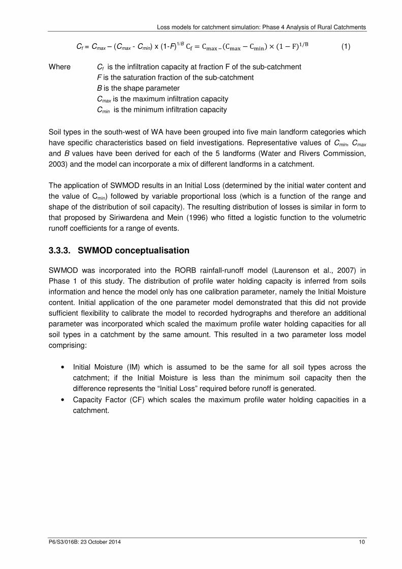
3.3.3. SWMOD conceptualisation
SWMOD was incorporated into the RORB rainfall-runoff model (Laurenson et al., 2007) in
Phase 1 of this study. The distribution of profile water holding capacity is inferred from soils
information and hence the model only has one calibration parameter, namely the Initial Moisture
content. Initial application of the one parameter model demonstrated that this did not provide
sufficient flexibility to calibrate the model to recorded hydrographs and therefore an additional
parameter was incorporated which scaled the maximum profile water holding capacities for all
soil types in a catchment by the same amount. This resulted in a two parameter loss model
comprising:
• Initial Moisture (IM) which is assumed to be the same for all soil types across the
catchment; if the Initial Moisture is less than the minimum soil capacity then the
difference represents the “Initial Loss” required before runoff is generated.
• Capacity Factor (CF) which scales the maximum profile water holding capacities in a
catchment.
Loss models for catchment simulation: Phase 4 Analysis of Rural Catchments
P6/S3/016B: 23 October 2014 11
Figure 3-3 Conceptualisation of 2 parameter SWMOD model
3.4. Estimation of profile water holding capacity
3.4.1. Introduction
In Australia, the application of distributed storage capacity models, such as SWMOD, in
Australia has historically been constrained by the lack of information on the hydraulic properties
of soils. The requirement of consistent data that can be applied across all Australian catchments
results in few options for characterising the soils for analysis.
The Atlas of Australian Soils (Northcote et al. 1960-1968) is the only consistent source of spatial
information for the whole of the country. McKenzie et al (2000) provide data on soil physical
properties for the 725 Principle Profile Forms (PPFs) identified in the Factual Key of Northcote
(1979) and the dominant PPFs for each soil landscape type in the Digital Atlas of Australian
Soils.
Properties provided by McKenzie et al. (2000) were estimated using a two-layer model of soil
using estimated characteristics for the A and B horizons. Estimates of thickness, texture, bulk
density and pedality were used to estimate parameters describing the soil water retention curve,
which then allow the calculation of the soil water holding capacity for each layer (McKenzie,
2000). Estimates were provided for the 5th percentile, median and 95th percentile.
Data extracted from the Atlas was used to characterise the soil storage capacity in each of the
study catchments. The 5th and 95th percentiles of A and B horizon thickness were taken as
approximates of the minimum and maximum thicknesses. The database provides a single A and
B horizon water holding capacity per unit depth for each soil type. The proportions of each soil
type in each pilot catchment was extracted from the Atlas and a distribution of catchment water
holding capacity was calculated using the distribution of soil horizon thickness and water holding
capacity.
So
il W
ate
r St
ora
ge
Fraction of area contributing to rainfall excess
Cmax
Cmin
β
CF > 1
CF < 1
IM
Loss models for catchment simulation: Phase 4 Analysis of Rural Catchments
P6/S3/016B: 23 October 2014 12
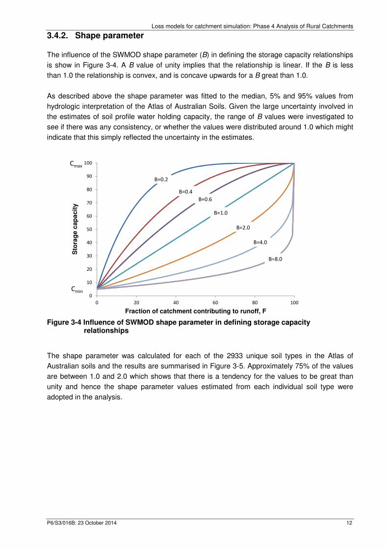
3.4.2. Shape parameter
The influence of the SWMOD shape parameter (B) in defining the storage capacity relationships
is show in Figure 3-4. A B value of unity implies that the relationship is linear. If the B is less
than 1.0 the relationship is convex, and is concave upwards for a B great than 1.0.
As described above the shape parameter was fitted to the median, 5% and 95% values from
hydrologic interpretation of the Atlas of Australian Soils. Given the large uncertainty involved in
the estimates of soil profile water holding capacity, the range of B values were investigated to
see if there was any consistency, or whether the values were distributed around 1.0 which might
indicate that this simply reflected the uncertainty in the estimates.
Figure 3-4 Influence of SWMOD shape parameter in defining storage capacity
relationships
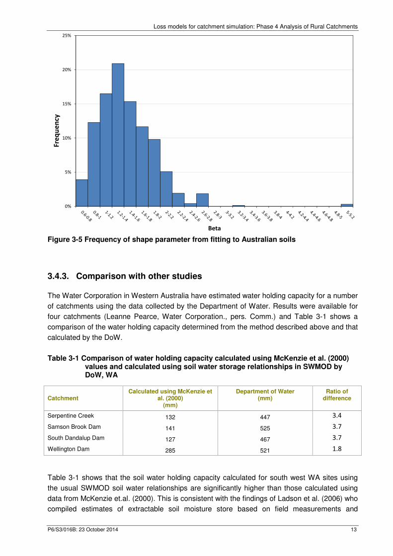
The shape parameter was calculated for each of the 2933 unique soil types in the Atlas of
Australian soils and the results are summarised in Figure 3-5. Approximately 75% of the values
are between 1.0 and 2.0 which shows that there is a tendency for the values to be great than
unity and hence the shape parameter values estimated from each individual soil type were
adopted in the analysis.
0
10
20
30
40
50
60
70
80
90
100
0 20 40 60 80 100
Sto
rag
e c
ap
acit
y
Fraction of catchment contributing to runoff, F
B=0.2
B=0.4
B=0.6
B=1.0
B=2.0
B=4.0
B=8.0
Cmax
Cmin
Loss models for catchment simulation: Phase 4 Analysis of Rural Catchments
P6/S3/016B: 23 October 2014 13
Figure 3-5 Frequency of shape parameter from fitting to Australian soils
3.4.3. Comparison with other studies
The Water Corporation in Western Australia have estimated water holding capacity for a number
of catchments using the data collected by the Department of Water. Results were available for
four catchments (Leanne Pearce, Water Corporation., pers. Comm.) and Table 3-1 shows a
comparison of the water holding capacity determined from the method described above and that
calculated by the DoW.
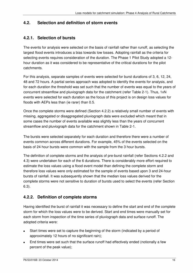
Table 3-1 Comparison of water holding capacity calculated using McKenzie et al. (2000) values and calculated using soil water storage relationships in SWMOD by DoW, WA
Catchment Calculated using McKenzie et
al. (2000) (mm)
Department of Water (mm)
Ratio of difference
Serpentine Creek 132 447 3.4
Samson Brook Dam 141 525 3.7
South Dandalup Dam 127 467 3.7
Wellington Dam 285 521 1.8
Table 3-1 shows that the soil water holding capacity calculated for south west WA sites using
the usual SWMOD soil water relationships are significantly higher than those calculated using
data from McKenzie et.al. (2000). This is consistent with the findings of Ladson et al. (2006) who
compiled estimates of extractable soil moisture store based on field measurements and
0%
5%
10%
15%
20%
25%
Fre
qu
en
cy
Beta

Loss models for catchment simulation: Phase 4 Analysis of Rural Catchments
P6/S3/016B: 23 October 2014 14
compared them with the soil moisture store from the Atlas. Results determined that 42% of
estimates from the Ladson et al. (2006) were greater than twice the value from the Atlas. In
general, they concluded that estimates of available water capacity from McKenzie et al. (2000)
could be considered a reasonable lower bound on field based estimates of the extractable soil
moisture.
Appendix G describes some sensitivity analysis undertaken after the completion of Stage 1 of
ARR Project #6. This confirmed that increasing the storage capacity values (in this case by a
nominal factor of 3) resulted in decreasing the value of the Capacity Factor. However, there was
no clear basis for adjusting the values and therefore in this study the storage capacity values
were adopted from McKenzie et al (2000) without modification.
Loss models for catchment simulation: Phase 4 Analysis of Rural Catchments
P6/S3/016B: 23 October 2014 15
4. Selection and characterisation of storm events
4.1. Embedded nature of design rainfall bursts
The rainfall data used in the derivation of Intensity Frequency Duration (IFD) information such as
IFD2013 (the new IFD information developed by the Bureau of Meteorology as part of the
revision of ARR; Green, et al. 2012) has been derived from the analysis of the most intense
bursts of rainfalls, rather than complete storms. The nature of these embedded bursts should be
accounted for when selecting loss values that are suitable for design (Hill and Mein, 1996; Rigby
and Bannigan, 1996).
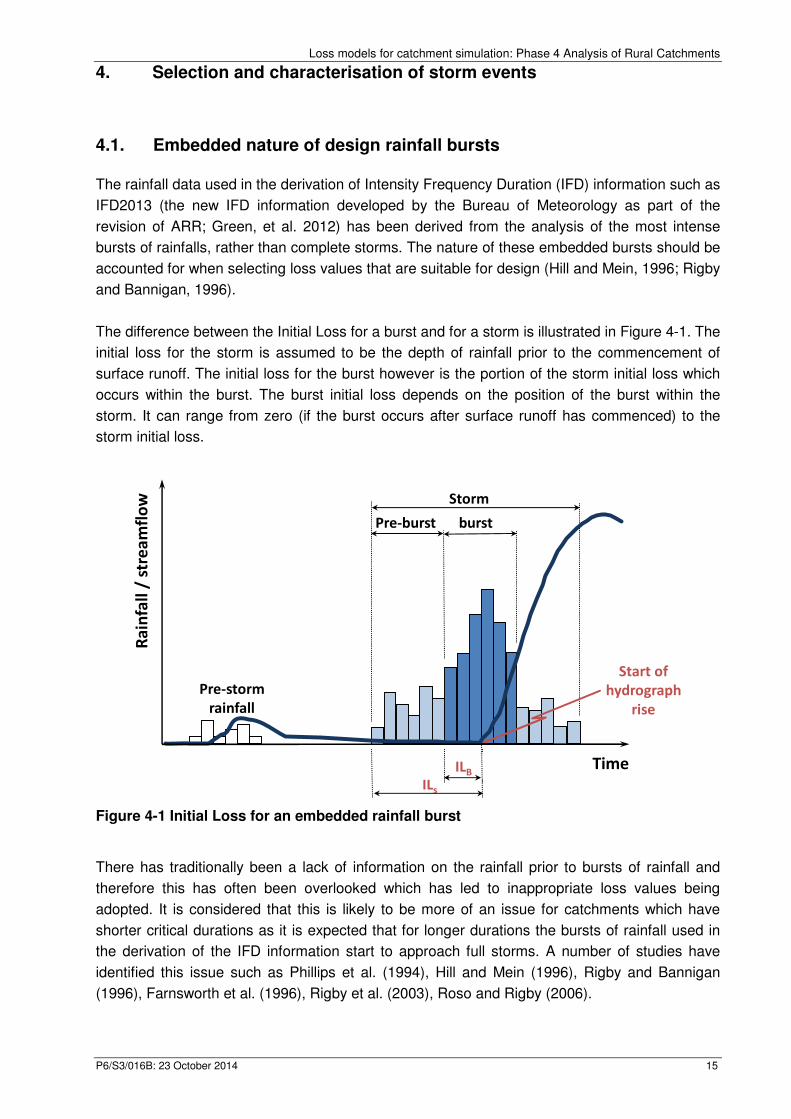
The difference between the Initial Loss for a burst and for a storm is illustrated in Figure 4-1. The
initial loss for the storm is assumed to be the depth of rainfall prior to the commencement of
surface runoff. The initial loss for the burst however is the portion of the storm initial loss which
occurs within the burst. The burst initial loss depends on the position of the burst within the
storm. It can range from zero (if the burst occurs after surface runoff has commenced) to the
storm initial loss.
Figure 4-1 Initial Loss for an embedded rainfall burst
There has traditionally been a lack of information on the rainfall prior to bursts of rainfall and
therefore this has often been overlooked which has led to inappropriate loss values being
adopted. It is considered that this is likely to be more of an issue for catchments which have
shorter critical durations as it is expected that for longer durations the bursts of rainfall used in
the derivation of the IFD information start to approach full storms. A number of studies have
identified this issue such as Phillips et al. (1994), Hill and Mein (1996), Rigby and Bannigan
(1996), Farnsworth et al. (1996), Rigby et al. (2003), Roso and Rigby (2006).
burstPre-burst
Storm
Time
Ra
infa
ll /
str
ea
mfl
ow
ILs
ILB
Start of
hydrograph
rise
Pre-storm
rainfall
Loss models for catchment simulation: Phase 4 Analysis of Rural Catchments
P6/S3/016B: 23 October 2014 16
4.2. Selection and definition of storm events
4.2.1. Selection of bursts
The events for analysis were selected on the basis of rainfall rather than runoff, as selecting the
largest flood events introduces a bias towards low losses. Adopting rainfall as the criteria for
selecting events requires consideration of the duration. The Phase 1 Pilot Study adopted a 12-
hour duration as it was considered to be representative of the critical durations for the pilot
catchments.
For this analysis, separate samples of events were selected for burst durations of 3, 6, 12, 24,
48 and 72 hours. A partial series approach was adopted to identify the events for analysis, and
for each duration the threshold was set such that the number of events was equal to the years of
concurrent streamflow and pluviograph data for the catchment (refer Table 2-1). Thus, 1xN
events were selected for each duration as the focus of this project is on design loss values for
floods with AEPs less than (ie rarer) than 0.5.
Once the complete storms were defined (Section 4.2.2) a relatively small number of events with
missing, aggregated or disaggregated pluviograph data were excluded which meant that in
some cases the number of events available was slightly less than the years of concurrent
streamflow and pluviograph data for the catchment shown in Table 2-1.
The bursts were selected separately for each duration and therefore there were a number of
events common across different durations. For example, 45% of the events selected on the
basis of 24 hour bursts were common with the sample from the 3 hour bursts.
The definition of complete storms and the analysis of pre-burst rainfall (refer Sections 4.2.2 and
4.3) were undertaken for each of the 6 durations. There is considerably more effort required to
estimate the loss values using a flood event model than defining the complete storm and
therefore loss values were only estimated for the sample of events based upon 3 and 24-hour
bursts of rainfall. It was subsequently shown that the median loss values derived for the
complete storms were not sensitive to duration of bursts used to select the events (refer Section
6.3).
4.2.2. Definition of complete storms
Having identified the burst of rainfall it was necessary to define the start and end of the complete
storm for which the loss values were to be derived. Start and end times were manually set for
each storm from inspection of the time series of pluviograph data and surface runoff. The
adopted criteria were:
� Start times were set to capture the beginning of the storm (indicated by a period of
approximately 12 hours of no significant rain);
� End times were set such that the surface runoff had effectively ended (notionally a few
percent of the peak value);
P6/S3/016B: 23 October 2014
� Start and end times were set to 9:00
the spatial distribution of rainfa
For some events it was not possible to satisfy all criteria and therefore start and end times were
based upon a compromise between
As discussed in Section 4.2.1
duration bursts. In these cases a
were adopted for the same storm.
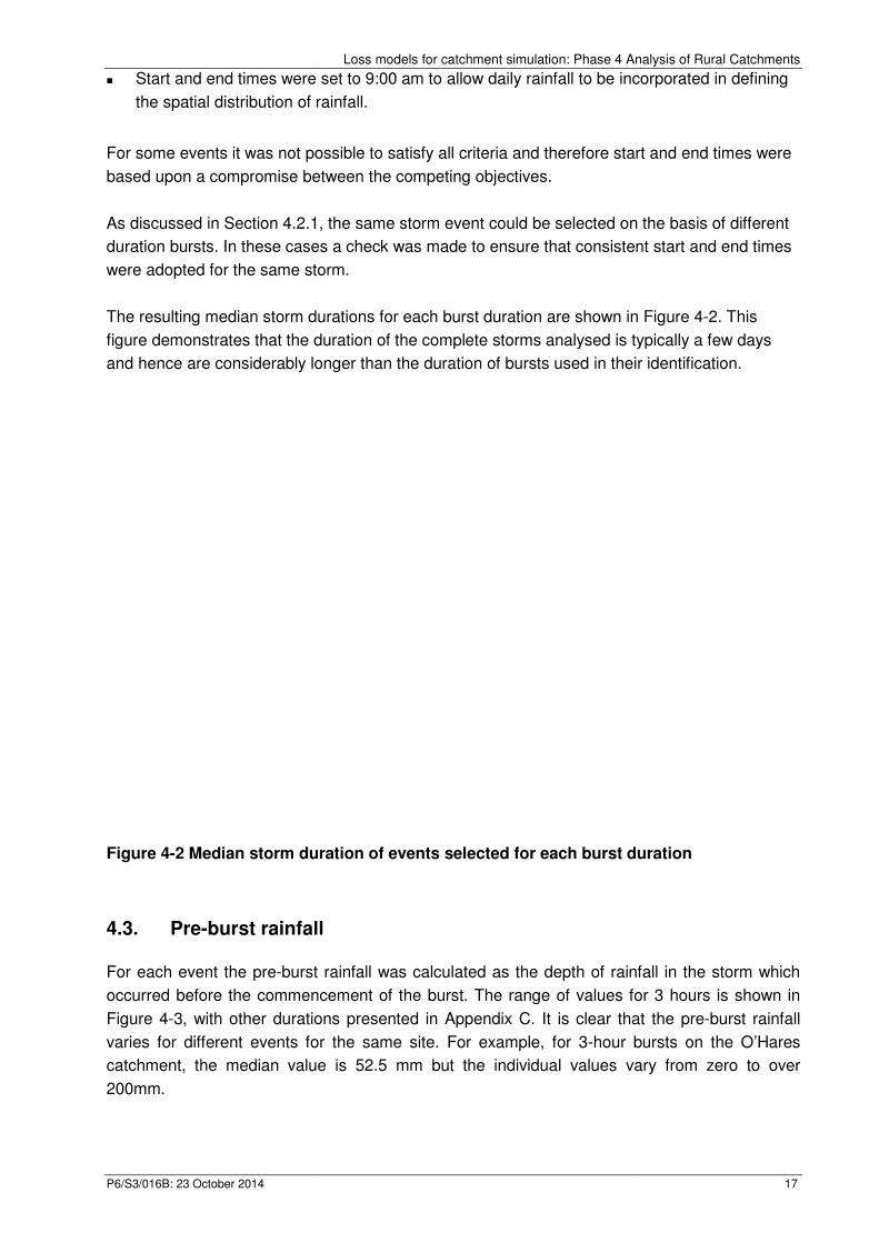
The resulting median storm duration
figure demonstrates that the duration of the complete storms analysed is typically a few days
and hence are considerably longer than the
Figure 4-2 Median storm duration of
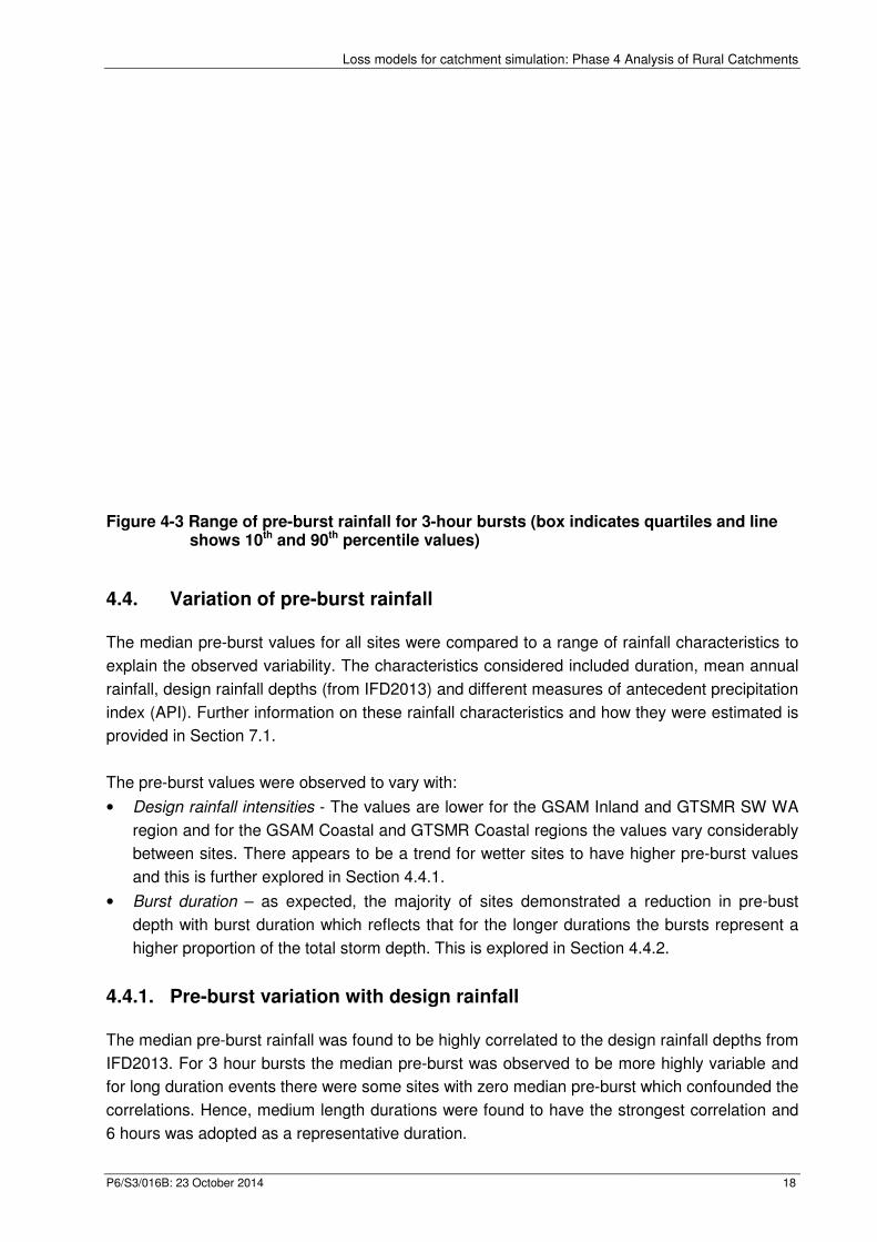
4.3. Pre-burst rainfall
For each event the pre-burst rainfall was calculated as the depth of rainfall in the storm which
occurred before the commencement of the burs
Figure 4-3, with other durations presented in
varies for different events for
catchment, the median value is
200mm.
Loss models for catchment simulation: Phase 4 Analysis of Rural Catchments
Start and end times were set to 9:00 am to allow daily rainfall to be incorporated in defining
the spatial distribution of rainfall.
For some events it was not possible to satisfy all criteria and therefore start and end times were
e between the competing objectives.
4.2.1, the same storm event could be selected on the basis of different
In these cases a check was made to ensure that consistent start and end times
for the same storm.
The resulting median storm durations for each burst duration are shown in
that the duration of the complete storms analysed is typically a few days
considerably longer than the duration of bursts used in their identification
Median storm duration of events selected for each burst duration
ainfall
burst rainfall was calculated as the depth of rainfall in the storm which
occurred before the commencement of the burst. The range of values for 3 hours is shown in
, with other durations presented in Appendix C. It is clear that the pre
varies for different events for the same site. For example, for 3-hour bursts on the
catchment, the median value is 52.5 mm but the individual values vary from zero to over
Loss models for catchment simulation: Phase 4 Analysis of Rural Catchments
17
am to allow daily rainfall to be incorporated in defining
For some events it was not possible to satisfy all criteria and therefore start and end times were
ected on the basis of different
check was made to ensure that consistent start and end times
are shown in Figure 4-2. This
that the duration of the complete storms analysed is typically a few days
bursts used in their identification.
selected for each burst duration
burst rainfall was calculated as the depth of rainfall in the storm which
The range of values for 3 hours is shown in
It is clear that the pre-burst rainfall
bursts on the O’Hares
mm but the individual values vary from zero to over
P6/S3/016B: 23 October 2014
Figure 4-3 Range of pre-burst rainfall for shows 10th and 90
4.4. Variation of pre-burst rainfall
The median pre-burst values for all
explain the observed variability. The characteristics considered in
rainfall, design rainfall depths (from IFD2013) and different measures of antecedent precipitation
index (API). Further information on these rainfall characteristics and how they were estimated is
provided in Section 7.1.
The pre-burst values were observed to vary with
• Design rainfall intensities
region and for the GSAM Coastal and GTSMR Coastal regions the values vary considerably
between sites. There appears to be a trend for wetter
and this is further explored in Section
• Burst duration – as expected
depth with burst duration which reflects that for the longer durations the bursts represent a
higher proportion of the total storm depth.
4.4.1. Pre-burst variation with
The median pre-burst rainfall was found to be highly correlated to the design rainfall depths from
IFD2013. For 3 hour bursts the median pre
for long duration events there were some
correlations. Hence, medium length durations were found to have the strongest correlation
6 hours was adopted as a representative duration
Loss models for catchment simulation: Phase 4 Analysis of Rural Catchments
urst rainfall for 3-hour bursts (box indicates and 90th percentile values)
burst rainfall
burst values for all sites were compared to a range of rainfall characteristics to
explain the observed variability. The characteristics considered included duration, mean annual
rainfall, design rainfall depths (from IFD2013) and different measures of antecedent precipitation
index (API). Further information on these rainfall characteristics and how they were estimated is
were observed to vary with:
- The values are lower for the GSAM Inland and GTSMR SW WA
the GSAM Coastal and GTSMR Coastal regions the values vary considerably
s. There appears to be a trend for wetter sites to have higher pre
and this is further explored in Section 4.4.1.
as expected, the majority of sites demonstrated a reduction in pre
ith burst duration which reflects that for the longer durations the bursts represent a
higher proportion of the total storm depth. This is explored in Section 4.4
burst variation with design rainfall
t rainfall was found to be highly correlated to the design rainfall depths from
the median pre-burst was observed to be more highly
uration events there were some sites with zero median pre-burst
Hence, medium length durations were found to have the strongest correlation
6 hours was adopted as a representative duration.
Loss models for catchment simulation: Phase 4 Analysis of Rural Catchments
18
es quartiles and line
range of rainfall characteristics to
cluded duration, mean annual
rainfall, design rainfall depths (from IFD2013) and different measures of antecedent precipitation
index (API). Further information on these rainfall characteristics and how they were estimated is
M Inland and GTSMR SW WA
the GSAM Coastal and GTSMR Coastal regions the values vary considerably
s to have higher pre-burst values
demonstrated a reduction in pre-bust
ith burst duration which reflects that for the longer durations the bursts represent a
4.4.2.
t rainfall was found to be highly correlated to the design rainfall depths from
more highly variable and
burst which confounded the
Hence, medium length durations were found to have the strongest correlation and
P6/S3/016B: 23 October 2014
No increase in regression performance was achieved through separation of data into GSAM and
GTMSR region. However, six
relatively high design rainfall
the 4 sites from the Northern Territory
WA. The remaining site that had zero median 6
Queensland. For this site nearly half of the values were non
non-zero median pre-burst. This site was therefore excluded as an outlier.
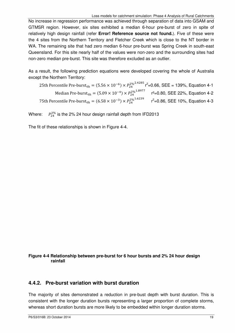
As a result, the following prediction equation
except the Northern Territory:
25thPercentilePre-burst
MedianPre-burst
75thPercentilePre-burst
Where: '()(% is the 2% 24 hour design rainfall depth from IFD2013
The fit of these relationships is shown in
Figure 4-4 Relationship betweenrainfall
4.4.2. Pre-burst variation with
The majority of sites demonstrated a reduction in pre
consistent with the longer duration bursts representing a larger proportion of complete storms,
whereas short duration bursts are more likely to be embedded within long
Loss models for catchment simulation: Phase 4 Analysis of Rural Catchments
No increase in regression performance was achieved through separation of data into GSAM and
However, six sites exhibited a median 6-hour pre-burst
(refer Error! Reference source not found.
from the Northern Territory and Fletcher Creek which is close to the NT border in
WA. The remaining site that had zero median 6-hour pre-burst was Spring Creek in south
Queensland. For this site nearly half of the values were non-zero and the surrounding sites had
burst. This site was therefore excluded as an outlier.
As a result, the following prediction equations were developed covering the whole of Australia
:
burst6h = �5.56 × 10�.� '()(%(.)(/0
r2=0.66, SEE =
burst6h � �5.09 10�)� '()(%�./233
r²=0.80, SEE 2
burst6h � �6.58 10�5� '()(%�..(52
r2=0.86, SEE
is the 2% 24 hour design rainfall depth from IFD2013
is shown in Figure 4-4.
Relationship between pre-burst for 6 hour bursts and 2% 24 hour design
ariation with burst duration
s demonstrated a reduction in pre-bust depth with burst duration. This is
consistent with the longer duration bursts representing a larger proportion of complete storms,
whereas short duration bursts are more likely to be embedded within longer duration storms.
Loss models for catchment simulation: Phase 4 Analysis of Rural Catchments
19
No increase in regression performance was achieved through separation of data into GSAM and
burst of zero in spite of
Error! Reference source not found.). Five of these were
close to the NT border in
burst was Spring Creek in south-east
zero and the surrounding sites had
burst. This site was therefore excluded as an outlier.
developed covering the whole of Australia
=0.66, SEE = 139%, Equation 4-1
SEE 22%, Equation 4-2
, SEE 10%, Equation 4-3
burst for 6 hour bursts and 2% 24 hour design
bust depth with burst duration. This is
consistent with the longer duration bursts representing a larger proportion of complete storms,
er duration storms.

P6/S3/016B: 23 October 2014
The variation of pre-burst depth with burst duration is plotted for each
example of the pre-burst rainfall for South Maroochy
This is typical of most sites
rainfall with burst duration.
Figure 4-5 Range of pre-burst rainfall for(box indicates quartiles and line show 10
However, there is more variability in the pre
the 3-hours is lower than the pre
shown in Figure 4-6 for McMahons in Victoria.
The variability in the pre-burst depths for 3 hour bursts is likely to be caused by different mixes
of storm mechanisms contributing to the rainfall with
isolated thunderstorms (associated with zero or very small pre
intense cells within much longer duration storms.
To explore this variability the ratio of median 3
compared to the rainfall characteristics defined in Section
of these characteristics could explain the observed variability.
variation across regions. It is recommended that this be
Loss models for catchment simulation: Phase 4 Analysis of Rural Catchments
burst depth with burst duration is plotted for each site
burst rainfall for South Maroochy in Queensland is presented in
and demonstrates the consistent reduction in median pre
burst rainfall for South Maroochy for each duratdicates quartiles and line show 10th and 90th percentile
there is more variability in the pre-burst for 3-hour bursts. For 8
is lower than the pre-burst associated with the 6-hour events. An
for McMahons in Victoria.
burst depths for 3 hour bursts is likely to be caused by different mixes
of storm mechanisms contributing to the rainfall with some 3-hour rainfalls being generated by
(associated with zero or very small pre-burst depths)
intense cells within much longer duration storms.
the ratio of median 3-hour pre-burst to median 6
compared to the rainfall characteristics defined in Section 7.1 (see Appendix D
of these characteristics could explain the observed variability. Similarly, there wa
It is recommended that this be investigated with a larger dataset.
Loss models for catchment simulation: Phase 4 Analysis of Rural Catchments
20
site in Appendix E. An
is presented in Figure 4-5.
and demonstrates the consistent reduction in median pre-burst
South Maroochy for each duration
percentile values)
or 8 sites the pre-burst for
hour events. An example of this is
burst depths for 3 hour bursts is likely to be caused by different mixes
r rainfalls being generated by
burst depths) whereas others are
burst to median 6-hour pre-burst was
Appendix D); however, none
Similarly, there was no obvious
with a larger dataset.
P6/S3/016B: 23 October 2014
Figure 4-6 Range of pre-burst rainfall for(box indicates quartiles and
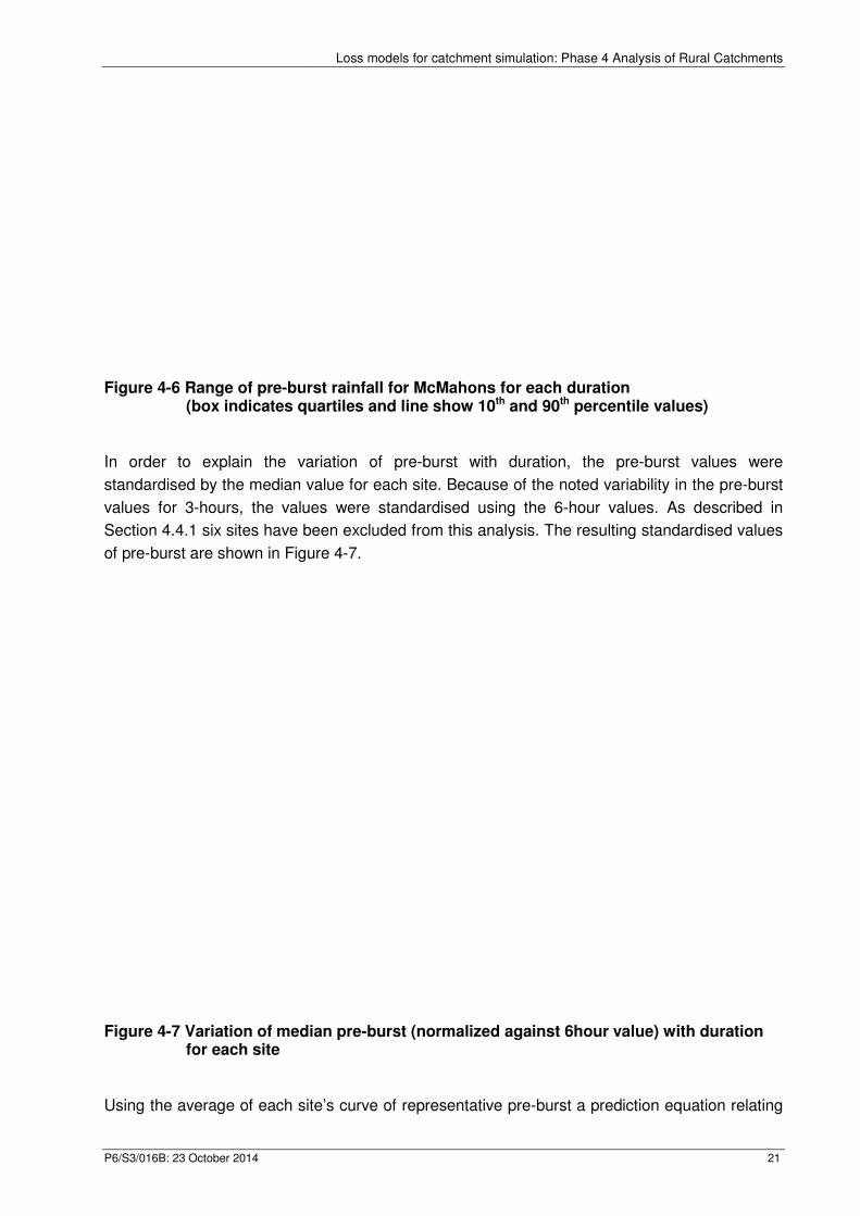
In order to explain the variation of pre
standardised by the median value for each
values for 3-hours, the values were standardised using the 6
Section 4.4.1 six sites have been excluded from this analysis.
of pre-burst are shown in Figure
Figure 4-7 Variation of median prefor each site
Using the average of each site’s
Loss models for catchment simulation: Phase 4 Analysis of Rural Catchments
burst rainfall for McMahons for each durationdicates quartiles and line show 10th and 90th percentile
In order to explain the variation of pre-burst with duration, the pre
by the median value for each site. Because of the noted variability in the pre
lues were standardised using the 6-hour values.
have been excluded from this analysis. The resulting standardised values
Figure 4-7.
Variation of median pre-burst (normalized against 6hour value)
site’s curve of representative pre-burst a prediction equation
Loss models for catchment simulation: Phase 4 Analysis of Rural Catchments
21
for each duration
percentile values)
burst with duration, the pre-burst values were
Because of the noted variability in the pre-burst
hour values. As described in
The resulting standardised values
(normalized against 6hour value) with duration
burst a prediction equation relating
P6/S3/016B: 23 October 2014
duration and pre-burst was defined:
Pre-burstduration � Pre
Where: duration is the duration of the burst in hours
Pre-burst6h is the median pre
For an ungauged catchment t
in Section 4.4.1 to estimate pre
4.4.3. Pre-burst as a pr
In the previous sections the pre
the pre-burst rainfall is considered as a p
ratio for all events in a particula
This shows that the ratio of pre
Additionally, pre-burst is larger relative to burst rainfall for the G
coastal sites. This is consistent with pre
Figure 4-3. The negligible pre
is further illustrated here.
Figure 4-8 Change in Pre-burst/burst rainfall ratio with duration for each regionand Fletcher Creek separated from GTSMR coastalexcluded)
Distribution summaries of pre
Loss models for catchment simulation: Phase 4 Analysis of Rural Catchments
was defined:
Pre-burst6h 7�8.8.)/�duration�.� r2=0.99, SEE 1
is the duration of the burst in hours
the median pre-burst depth in mm for a 6 hour burst
For an ungauged catchment this relationship can be used in conjunction with
to estimate pre-burst for each duration.
roportion of burst depth
In the previous sections the pre-burst has been expressed as an absolute value. In this section
burst rainfall is considered as a proportion of the burst rainfall. The median values of the
ratio for all events in a particular region are summarised in Figure 4-8.
This shows that the ratio of pre-burst to burst rainfall reduces with increasing
burst is larger relative to burst rainfall for the GTMSR coastal and G
. This is consistent with pre-burst being larger for wetter catchments, as seen in
The negligible pre-burst for the Northern Territory sites as described in Section
burst/burst rainfall ratio with duration for each regionand Fletcher Creek separated from GTSMR coastal sites, and
of pre-burst normalized against burst rainfall for each region can be
Loss models for catchment simulation: Phase 4 Analysis of Rural Catchments
22
SEE 18%, Equation 4-4
burst depth in mm for a 6 hour burst
his relationship can be used in conjunction with the regionalization
burst has been expressed as an absolute value. In this section
roportion of the burst rainfall. The median values of the
increasing burst duration.
astal and GSAM
burst being larger for wetter catchments, as seen in
as described in Section 4.4.1
burst/burst rainfall ratio with duration for each region (NT sites , and Spring Creek
burst normalized against burst rainfall for each region can be
P6/S3/016B: 23 October 2014
found in Appendix F.
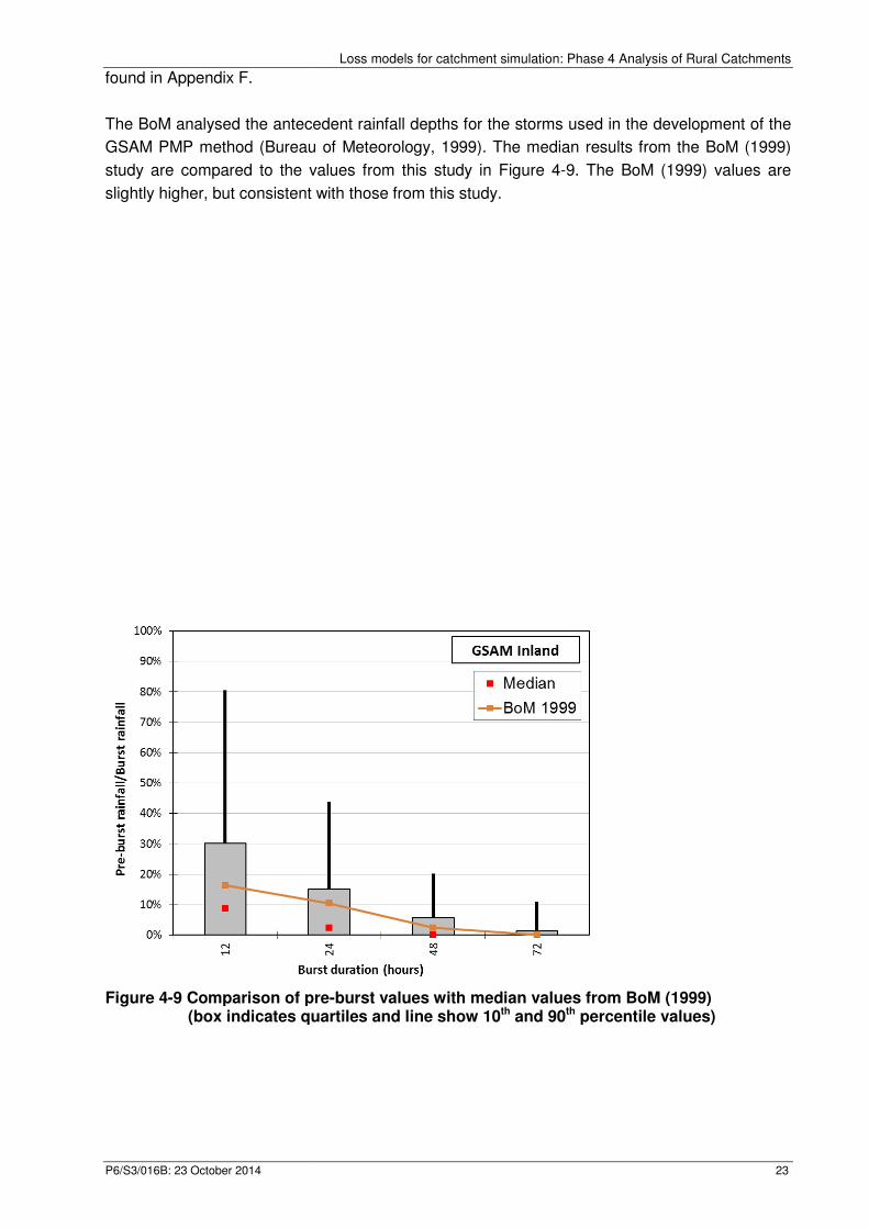
The BoM analysed the antecedent rainfall depths for the storms used in t
GSAM PMP method (Bureau of Meteorology, 1999).
study are compared to the values from this study in
slightly higher, but consistent with those from this study.
Figure 4-9 Comparison of pre(box indicates quartiles and line show 10
Loss models for catchment simulation: Phase 4 Analysis of Rural Catchments
The BoM analysed the antecedent rainfall depths for the storms used in t
GSAM PMP method (Bureau of Meteorology, 1999). The median results from the BoM (1999)
study are compared to the values from this study in Figure 4-9. The BoM (1999) values are
but consistent with those from this study.
Comparison of pre-burst values with median values from BoM (1999)dicates quartiles and line show 10th and 90th percentile
Loss models for catchment simulation: Phase 4 Analysis of Rural Catchments
23
The BoM analysed the antecedent rainfall depths for the storms used in the development of the
The median results from the BoM (1999)
The BoM (1999) values are
burst values with median values from BoM (1999) percentile values)

P6/S3/016B: 23 October 2014
4.4.4. Pre-burst variation with burst severity
The ratio of pre-burst to burst rainfall is plotted against the Average Recurrence Interval (ARI) of
the burst for the 3 hour events
ratio to vary with the severity of the burst
proportion of the burst depth.
Figure 4-10 Relationship between ratio of prehour bursts. (Northern Territory catchments and Fletcher Creek separated from GTSMR coastal
Loss models for catchment simulation: Phase 4 Analysis of Rural Catchments
st variation with burst severity
burst to burst rainfall is plotted against the Average Recurrence Interval (ARI) of
for the 3 hour events in Figure 4-10. It is shown that there is no sig
ratio to vary with the severity of the burst, which implies that the pre-burst rainfall is a fixed
Relationship between ratio of pre-burst rainfall and burst ra(Northern Territory catchments and Fletcher Creek separated
from GTSMR coastal catchments, and Spring Creek excluded)
Loss models for catchment simulation: Phase 4 Analysis of Rural Catchments
24
burst to burst rainfall is plotted against the Average Recurrence Interval (ARI) of
significant trend for the
burst rainfall is a fixed
urst rainfall and burst rainfall to ARI for 3-(Northern Territory catchments and Fletcher Creek separated
, and Spring Creek excluded)
Loss models for catchment simulation: Phase 4 Analysis of Rural Catchments
P6/S3/016B: 23 October 2014 25
5. Estimation of loss values
This section describes the approach used to estimate loss values. The overall approach was
developed and trailed during Stage 1 of ARR Project #6 (SKM, 2012b). Some of the details were
further refined as part of a sensitivity analysis undertaken after Stage 1 and these results are
documented in Appendix G. This work highlighted the importance of ensuring that the volume of
surface runoff is maintained when estimating the loss values and hence the overall shaper and
volume was given more weight than the peak as outlined in Section 5.2.
5.1. Baseflow separation
Recorded streamflow is made up of baseflow, which is sourced from groundwater aquifers, and
quickflow, which is sourced from surface runoff. The usual method to remove baseflow involves
a subjective process of looking at the surface runoff and extracting baseflow based on
descriptions such as Nathan and McMahon (1990) and Brodie and Hostetler (2005). Manual
baseflow extraction for a large number of events for each of the catchments would be time
consuming, and so this process was automated by using a recursive digital filter. Further
information on the approach is contained in the ARR Project #7 report (SKM, 2011). The filter
parameter was fixed at 0.925 and the number of passes was set to 7 or 9 to provide a realistic
separation of baseflow. A summary of the adopted baseflow parameters is contained in
Appendix H.
5.2. Method
As part of the Phase 1 Pilot Study a preliminary attempt was made to develop lag relationships
which could be applied to the recorded streamflow data to directly estimate the losses. This
involved defining a threshold flow above which IL was deemed to be satisfied and then the CL or
PL was calculated from a water balance. Such an approach (without the allowance for lag) has
previously been applied by Hill et al (1996) and Ilahee (2005) to derive loss values for South-
East Australia and Queensland respectively. However, the investigation demonstrated the
difficulty in defining a single threshold that reproduces the loss values estimated using flood
models.
This reinforced the complexity of identifying the loss from the analysis of rainfall and surface
runoff and the importance of utilising a rainfall-runoff model. Therefore, loss values were derived
for the large number of events using a simplified calibration procedure which utilised a flood
event model.
The RORB rainfall-runoff model was selected as regional prediction equations for its
parameterisation are readily available for most regions in Australia. RORB is a general runoff
and streamflow routing program that is used to calculate flood hydrographs from rainfall and
other catchment and channel inputs. The model subtracts losses from rainfall to determine
rainfall excess and routes this through catchment storages represented by the stream length to
produce streamflow hydrographs at points of interest. The model can account for both temporal
and spatial distribution of rainfall and losses.
The model is based on catchment geometry and topographic data, and the two principal
parameters are kc and m. The parameter m describes the degree of non-linearity of the
Loss models for catchment simulation: Phase 4 Analysis of Rural Catchments
P6/S3/016B: 23 October 2014 26
catchment’s response to rainfall excess and was set to 0.8 based upon the recommendations in
ARR. The parameter kc describes the delay in the catchment’s response to rainfall excess.
The RORB catchment file requires information about the catchment layout, which is obtained by
delineating the catchment into smaller sub-areas that are joined by reaches. The 1 to 25,000
spatial information from the Bureau of Meteorology geofabric was used as a basis for
delineating the catchments. The geofabric network information and cartographic layers were
used to assist in developing sub-area boundaries and reaches. When delineating the catchment,
care was taken to include at least 5 sub-areas upstream of the catchment outlet, and to make
the sub-areas a similar size. The catchment boundaries derived using the geofabric information
was checked against those reported by the relevant agencies.
As part of scoping the work for Phase 4 a sensitivity analysis was undertaken to test whether the
loss values are sensitive to the adopted structure of the routing model. For 5 catchments, losses
were estimated using RORB and also an URBS model with separate routing parameters for
channel and overland routing (α and β). The results are included in Appendix G4 and
demonstrate that the results are not sensitive to the selection of routing model.
The following simplifications were incorporated:
� Spatial patterns – the spatial distribution of rainfall for each event was derived from inverse-
distance weighting of nearby daily rainfall stations rather than manually deriving isohyets.
� Fixed routing parameter – for each loss model the routing parameter kc was kept fixed for
every event on a catchment.
� Timing – the temporal distribution of rainfall and streamflow was adopted without
adjustment.
� Baseflow separation – the contribution of baseflow to each event was estimated using the
recursive digital filter and the parameters summarised in Appendix H rather than manually
estimate the baseflow.
Based upon the above simplifications, RORB was used to estimate the values of IL/CL and
SWMOD for each of the events identified in Section 4.2.1. The estimation of loss values
required subjective fitting of the modelled hydrograph with the surface runoff estimated from
subtracting the baseflow from the recorded total streamflow.
In reviewing the results from the Phase 1 Pilot Study it was noted that undue weight was given
to fitting the peaks at the expense of the volume and there was a tendency to underestimate the
flood volume (refer Appendix G). Hence in Phase 4 greater emphasis was placed on the volume
and the following criteria (from most to least important) were adopted:
� Overall shape
� Volume
� Timing
� Peak
In many cases, the fit could have been improved by adjusting the routing parameter but the fits
were deemed to be appropriate for estimating the loss values for the event.
Loss models for catchment simulation: Phase 4 Analysis of Rural Catchments
P6/S3/016B: 23 October 2014 27
5.3. Review of loss values
Because the events were selected on the basis of rainfall, some events yielded little or no
surface runoff and this confounded the estimation of loss parameters. Where no surface runoff
was generated the event was excluded as it was not possible to estimate the IL value; all that
could be determined was that the value was at least the depth of rainfall. For events which
yielded a small surface runoff (typically less than a few m³/s) it was often difficult to obtain a
good match between the modelled and surface runoff estimated from the recorded flow data. In
these cases the event was discarded as they were subject to considerable uncertainty.
For each event a subjective score from 0 to 9 was assigned based upon the goodness of fits
giving consideration to the criteria listed above. An example of the fits is provided in Figure 5-1.
For each catchment, the sample of events was reviewed and outliers or events considered to be
highly uncertain were removed. Events were excluded if::
• Volume errors were large (as indicated by zero CL and significant underestimation of
volume, typically 20%)
• Runoffs were very low (typically 1.0m³/s but this threshold was increased for some
catchments)
• There was a mismatch in timing between rainfall and runoff
• the fit between calculated and recorded hydrographs was very poor
• The fitted value of CL was abnormally high (typically > 20 mm/h)
• The fitted value of CF was abnormally high (typically > 10)
• The complete period of rainfall was very short (typically less than 3 hours) which made
the identification of loss values problematic given the 1 hour time step.
Typically more events were removed from the sample selected by 3-hour rather than 24-hour
bursts. Therefore unless otherwise indicated, the analysis and presentation of results in the
following sections has focussed on the sample selected from 24-hour bursts.

P6/S3/016B: 23 October 2014
Figure 5-1 Example skill scores used to assess goodness of fit between calculated and recorded hydrographs
Loss models for catchment simulation: Phase 4 Analysis of Rural Catchments
scores used to assess goodness of fit between calculated and recorded hydrographs
Loss models for catchment simulation: Phase 4 Analysis of Rural Catchments
28
scores used to assess goodness of fit between calculated and
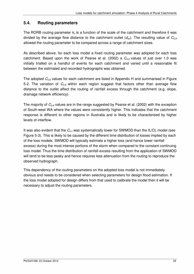
Loss models for catchment simulation: Phase 4 Analysis of Rural Catchments
P6/S3/016B: 23 October 2014 29
5.4. Routing parameters
The RORB routing parameter kc is a function of the scale of the catchment and therefore it was
divided by the average flow distance to the catchment outlet (dav). The resulting value of C0.8
allowed the routing parameter to be compared across a range of catchment sizes.
As described above, for each loss model a fixed routing parameter was adopted for each loss
catchment. Based upon the work of Pearse et al. (2002) a C0.8 values of just over 1.0 was
initially trialled on a handful of events for each catchment and varied until a reasonable fit
between the estimated and recorded hydrographs was obtained.
The adopted C0.8 values for each catchment are listed in Appendix H and summarised in Figure
5-2. The variation of C0.8 within each region suggest that factors other than average flow
distance to the outlet affect the routing of rainfall excess through the catchment (e.g. slope,
drainage network efficiency).
The majority of C0.8 values are in the range suggested by Pearse et al. (2002) with the exception
of South-west WA where the values were consistently higher. This indicates that the catchment
response is different to other regions in Australia and is likely to be characterised by higher
levels of interflow.
It was also evident that the C0.8 was systematically lower for SWMOD than the IL/CL model (see
Figure 5-3). This is likely to be caused by the different time distribution of losses implied by each
of the loss models. SWMOD will typically estimate a higher loss (and hence lower rainfall
excess) during the most intense portions of the storm when compared to the constant continuing
loss model. Thus the time distribution of rainfall excess resulting from the application of SWMOD
will tend to be less peaky and hence requires less attenuation from the routing to reproduce the
observed hydrograph.
This dependency of the routing parameters on the adopted loss model is not immediately
obvious and needs to be considered when selecting parameters for design flood estimation. If
the loss model adopted for design differs from that used to calibrate the model then it will be
necessary to adjust the routing parameters.
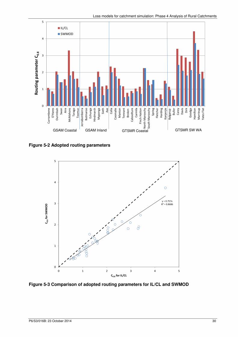
Loss models for catchment simulation: Phase 4 Analysis of Rural Catchments
P6/S3/016B: 23 October 2014 30
Figure 5-2 Adopted routing parameters
Figure 5-3 Comparison of adopted routing parameters for IL/CL and SWMOD
0
1
2
3
4
5
Cu
rra
mb
en
e
O'H
are
s
Ou
rim
ba
h
Swa
n
Air
e
McM
ah
on
s
Ta
rag
o
To
om
uc
Jerr
ab
om
be
rra
Bu
tma
roo
Ech
un
ga
Hin
dm
ars
h
Myp
on
ga
Six
th
Axe
Ce
lia
Co
om
ali
e
Ma
nto
n
Te
nn
an
t
Bro
ken
Ca
bo
olt
ure
Ca
rmil
a
Fin
ch H
att
on
No
rth
Ma
roo
chy
So
uth
Ma
roo
chy
Spri
ng
Fle
tch
er
Ha
rdin
g
Ka
nje
nji
e
Ba
lga
rup
Bu
ller
Ca
rey
Da
vis
Dir
k
Go
od
ga
Ha
milt
on
Ma
rrin
up
Ya
tes
Fla
t
Ro
uti
ng
pa
ram
ete
r C
0.8
IL/CL
SWMOD
GSAM Coastal GSAM Inland GTSMR Coastal GTSMR SW WA
y = 0.757x
R² = 0.8686
0
1
2
3
4
5
0 1 2 3 4 5
C0
.8fo
r S
WM
OD
C0.8 for IL/CL
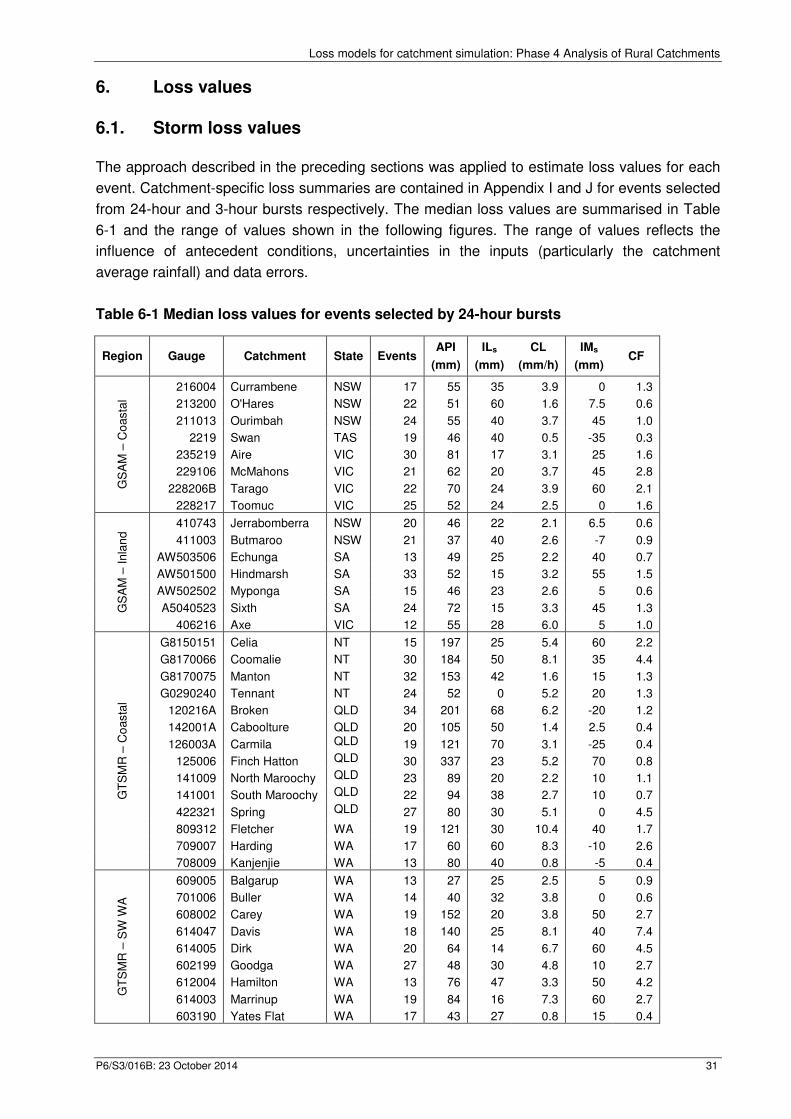
Loss models for catchment simulation: Phase 4 Analysis of Rural Catchments
P6/S3/016B: 23 October 2014 31
6. Loss values
6.1. Storm loss values
The approach described in the preceding sections was applied to estimate loss values for each
event. Catchment-specific loss summaries are contained in Appendix I and J for events selected
from 24-hour and 3-hour bursts respectively. The median loss values are summarised in Table
6-1 and the range of values shown in the following figures. The range of values reflects the
influence of antecedent conditions, uncertainties in the inputs (particularly the catchment
average rainfall) and data errors.
Table 6-1 Median loss values for events selected by 24-hour bursts
Region Gauge Catchment State Events API
(mm)
ILs
(mm)
CL
(mm/h)
IMs
(mm) CF
GS
AM
– C
oasta
l
216004 Currambene NSW 17 55 35 3.9 0 1.3
213200 O'Hares NSW 22 51 60 1.6 7.5 0.6
211013 Ourimbah NSW 24 55 40 3.7 45 1.0
2219 Swan TAS 19 46 40 0.5 -35 0.3
235219 Aire VIC 30 81 17 3.1 25 1.6
229106 McMahons VIC 21 62 20 3.7 45 2.8
228206B Tarago VIC 22 70 24 3.9 60 2.1
228217 Toomuc VIC 25 52 24 2.5 0 1.6
GS
AM
– I
nla
nd 410743 Jerrabomberra NSW 20 46 22 2.1 6.5 0.6
411003 Butmaroo NSW 21 37 40 2.6 -7 0.9
AW503506 Echunga SA 13 49 25 2.2 40 0.7
AW501500 Hindmarsh SA 33 52 15 3.2 55 1.5
AW502502 Myponga SA 15 46 23 2.6 5 0.6
A5040523 Sixth SA 24 72 15 3.3 45 1.3
406216 Axe VIC 12 55 28 6.0 5 1.0
GT
SM
R –
Co
asta
l
G8150151 Celia NT 15 197 25 5.4 60 2.2
G8170066 Coomalie NT 30 184 50 8.1 35 4.4
G8170075 Manton NT 32 153 42 1.6 15 1.3
G0290240 Tennant NT 24 52 0 5.2 20 1.3
120216A Broken QLD 34 201 68 6.2 -20 1.2
142001A Caboolture QLD 20 105 50 1.4 2.5 0.4
126003A Carmila QLD 19 121 70 3.1 -25 0.4
125006 Finch Hatton QLD 30 337 23 5.2 70 0.8
141009 North Maroochy QLD 23 89 20 2.2 10 1.1
141001 South Maroochy QLD 22 94 38 2.7 10 0.7
422321 Spring QLD 27 80 30 5.1 0 4.5
809312 Fletcher WA 19 121 30 10.4 40 1.7
709007 Harding WA 17 60 60 8.3 -10 2.6
708009 Kanjenjie WA 13 80 40 0.8 -5 0.4
GT
SM
R –
SW
WA
609005 Balgarup WA 13 27 25 2.5 5 0.9
701006 Buller WA 14 40 32 3.8 0 0.6
608002 Carey WA 19 152 20 3.8 50 2.7
614047 Davis WA 18 140 25 8.1 40 7.4
614005 Dirk WA 20 64 14 6.7 60 4.5
602199 Goodga WA 27 48 30 4.8 10 2.7
612004 Hamilton WA 13 76 47 3.3 50 4.2
614003 Marrinup WA 19 84 16 7.3 60 2.7
603190 Yates Flat WA 17 43 27 0.8 15 0.4
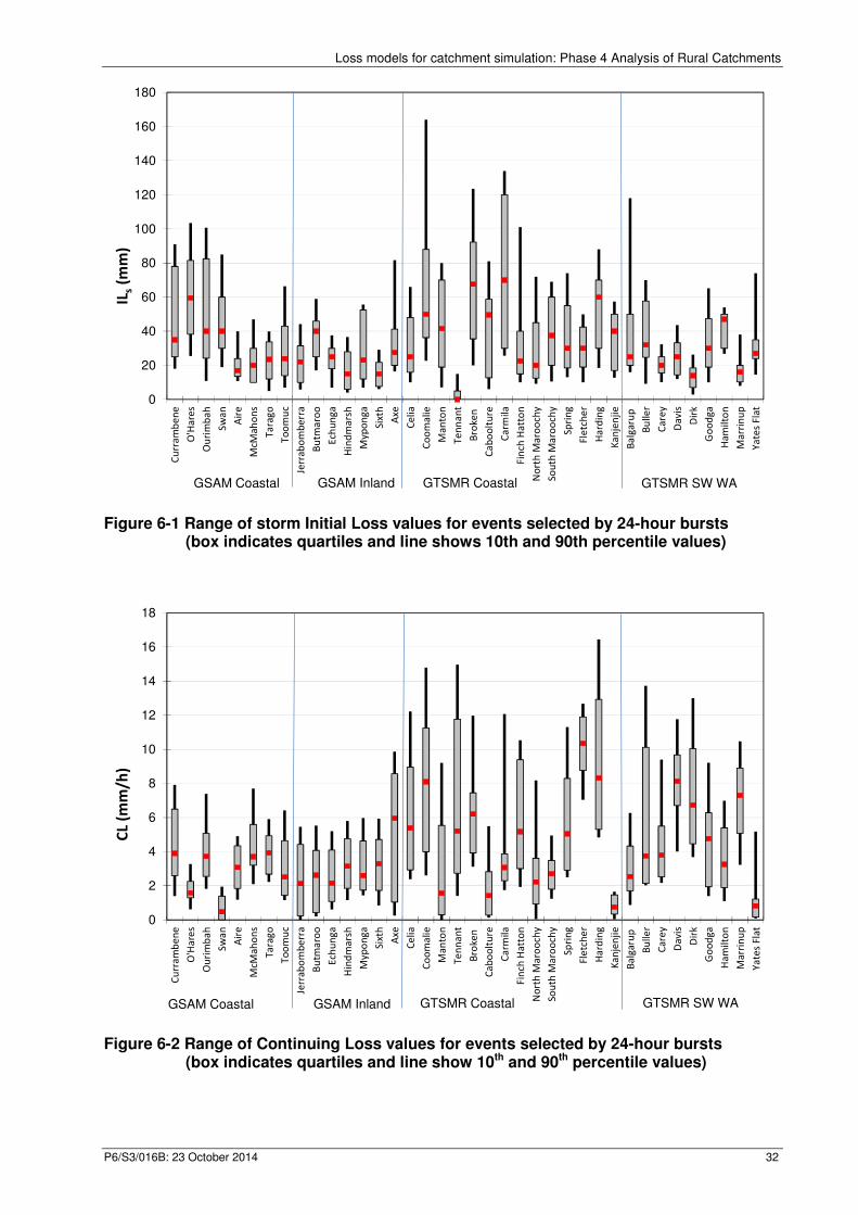
Loss models for catchment simulation: Phase 4 Analysis of Rural Catchments
P6/S3/016B: 23 October 2014 32
Figure 6-1 Range of storm Initial Loss values for events selected by 24-hour bursts (box indicates quartiles and line shows 10th and 90th percentile values)
Figure 6-2 Range of Continuing Loss values for events selected by 24-hour bursts
(box indicates quartiles and line show 10th and 90th percentile values)
0
20
40
60
80
100
120
140
160
180
Cu
rra
mb
en
e
O'H
are
s
Ou
rim
ba
h
Sw
an
Air
e
McM
ah
on
s
Ta
rag
o
To
om
uc
Jerr
ab
om
be
rra
Bu
tma
roo
Ech
un
ga
Hin
dm
ars
h
Myp
on
ga
Sixt
h
Axe
Ce
lia
Co
om
alie
Ma
nto
n
Te
nn
an
t
Bro
ken
Ca
bo
olt
ure
Ca
rmila
Fin
ch H
att
on
No
rth
Ma
roo
chy
Sou
th M
aro
och
y
Spri
ng
Fle
tch
er
Ha
rdin
g
Ka
nje
nji
e
Ba
lga
rup
Bu
ller
Ca
rey
Da
vis
Dir
k
Go
od
ga
Ha
mil
ton
Ma
rrin
up
Ya
tes
Fla
t
ILs
(mm
)
GSAM Coastal GSAM Inland GTSMR Coastal GTSMR SW WA
0
2
4
6
8
10
12
14
16
18
Cu
rra
mb
en
e
O'H
are
s
Ou
rim
ba
h
Sw
an
Air
e
McM
ah
on
s
Ta
rag
o
To
om
uc
Jerr
ab
om
be
rra
Bu
tma
roo
Ech
un
ga
Hin
dm
ars
h
Myp
on
ga
Sixt
h
Axe
Ce
lia
Co
om
alie
Ma
nto
n
Te
nn
an
t
Bro
ken
Ca
bo
olt
ure
Ca
rmila
Fin
ch H
att
on
No
rth
Ma
roo
chy
Sou
th M
aro
och
y
Spri
ng
Fle
tch
er
Ha
rdin
g
Ka
nje
nji
e
Ba
lga
rup
Bu
ller
Ca
rey
Da
vis
Dir
k
Go
od
ga
Ha
mil
ton
Ma
rrin
up
Ya
tes
Fla
t
CL
(mm
/h)
GSAM Coastal GSAM Inland GTSMR Coastal GTSMR SW WA
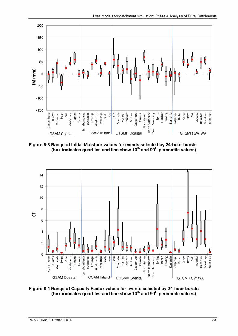
Loss models for catchment simulation: Phase 4 Analysis of Rural Catchments
P6/S3/016B: 23 October 2014 33
Figure 6-3 Range of Initial Moisture values for events selected by 24-hour bursts
(box indicates quartiles and line show 10th and 90th percentile values)
Figure 6-4 Range of Capacity Factor values for events selected by 24-hour bursts (box indicates quartiles and line show 10th and 90th percentile values)
-150
-100
-50
0
50
100
150
200
Cu
rra
mb
en
e
O'H
are
s
Ou
rim
ba
h
Swa
n
Air
e
McM
ah
on
s
Ta
rag
o
To
om
uc
Jerr
ab
om
be
rra
Bu
tma
roo
Ech
un
ga
Hin
dm
ars
h
Myp
on
ga
Six
th
Axe
Ce
lia
Co
om
ali
e
Ma
nto
n
Te
nn
an
t
Bro
ken
Ca
bo
olt
ure
Ca
rmil
a
Fin
ch H
att
on
No
rth
Ma
roo
chy
So
uth
Ma
roo
chy
Spri
ng
Fle
tch
er
Ha
rdin
g
Ka
nje
nji
e
Ba
lga
rup
Bu
ller
Ca
rey
Da
vis
Dir
k
Go
od
ga
Ha
milt
on
Ma
rrin
up
Ya
tes
Fla
t
IM (
mm
)
GSAM Coastal GSAM Inland GTSMR Coastal GTSMR SW WA
0
2
4
6
8
10
12
14
Cu
rra
mb
en
e
O'H
are
s
Ou
rim
ba
h
Swa
n
Air
e
McM
ah
on
s
Ta
rag
o
To
om
uc
Jerr
ab
om
be
rra
Bu
tma
roo
Ech
un
ga
Hin
dm
ars
h
Myp
on
ga
Six
th
Axe
Ce
lia
Co
om
ali
e
Ma
nto
n
Te
nn
an
t
Bro
ken
Ca
bo
olt
ure
Ca
rmil
a
Fin
ch H
att
on
No
rth
Ma
roo
chy
So
uth
Ma
roo
chy
Spri
ng
Fle
tch
er
Ha
rdin
g
Ka
nje
nji
e
Ba
lga
rup
Bu
ller
Ca
rey
Da
vis
Dir
k
Go
od
ga
Ha
milt
on
Ma
rrin
up
Ya
tes
Fla
t
CF
GSAM Coastal GSAM Inland GTSMR Coastal GTSMR SW WA
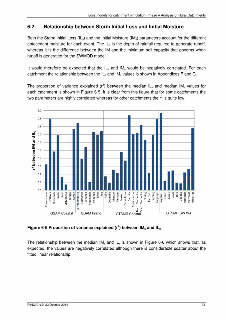
Loss models for catchment simulation: Phase 4 Analysis of Rural Catchments
P6/S3/016B: 23 October 2014 34
6.2. Relationship between Storm Initial Loss and Initial Moisture
Both the Storm Initial Loss (ILs) and the Initial Moisture (IMs) parameters account for the different
antecedent moisture for each event. The ILs is the depth of rainfall required to generate runoff,
whereas it is the difference between the IM and the minimum soil capacity that governs when
runoff is generated for the SWMOD model.
It would therefore be expected that the ILs and IMs would be negatively correlated. For each
catchment the relationship between the ILs and IMs values is shown in Appendices F and G.
The proportion of variance explained (r2) between the median ILs and median IMs values for
each catchment is shown in Figure 6-5. It is clear from this figure that for some catchments the
two parameters are highly correlated whereas for other catchments the r2 is quite low.
Figure 6-5 Proportion of variance explained (r2) between IMs and ILs
The relationship between the median IMs and ILs is shown in Figure 6-6 which shows that, as
expected, the values are negatively correlated although there is considerable scatter about the
fitted linear relationship.
0.0
0.1
0.2
0.3
0.4
0.5
0.6
0.7
0.8
0.9
1.0
Cu
rra
mb
en
e
O'H
are
s
Ou
rim
ba
h
Swa
n
Air
e
McM
ah
on
s
Ta
rag
o
To
om
uc
Jerr
ab
om
be
rra
Bu
tma
roo
Ech
un
ga
Hin
dm
ars
h
Myp
on
ga
Sixt
h
Axe
Ce
lia
Co
om
ali
e
Ma
nto
n
Te
nn
an
t
Bro
ken
Ca
bo
olt
ure
Ca
rmil
a
Fin
ch H
att
on
No
rth
Ma
roo
chy
Sou
th M
aro
och
y
Spri
ng
Fle
tch
er
Ha
rdin
g
Ka
nje
nji
e
Ba
lga
rup
Bu
ller
Ca
rey
Da
vis
Dir
k
Go
od
ga
Ha
mil
ton
Ma
rrin
up
Ya
tes
Fla
t
r2b
etw
ee
n I
M a
nd
IL s
GSAM Coastal GSAM Inland GTSMR Coastal GTSMR SW WA
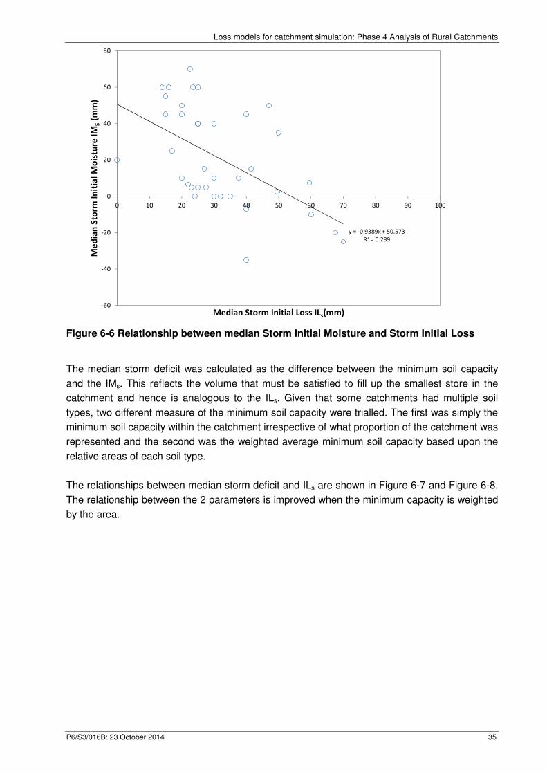
Loss models for catchment simulation: Phase 4 Analysis of Rural Catchments
P6/S3/016B: 23 October 2014 35
Figure 6-6 Relationship between median Storm Initial Moisture and Storm Initial Loss
The median storm deficit was calculated as the difference between the minimum soil capacity
and the IMs. This reflects the volume that must be satisfied to fill up the smallest store in the
catchment and hence is analogous to the ILs. Given that some catchments had multiple soil
types, two different measure of the minimum soil capacity were trialled. The first was simply the
minimum soil capacity within the catchment irrespective of what proportion of the catchment was
represented and the second was the weighted average minimum soil capacity based upon the
relative areas of each soil type.
The relationships between median storm deficit and ILs are shown in Figure 6-7 and Figure 6-8.
The relationship between the 2 parameters is improved when the minimum capacity is weighted
by the area.
y = -0.9389x + 50.573
R² = 0.289
-60
-40
-20
0
20
40
60
80
0 10 20 30 40 50 60 70 80 90 100
Me
dia
n S
torm
In
itia
l M
ois
ture
IM
S(m
m)
Median Storm Initial Loss ILs(mm)
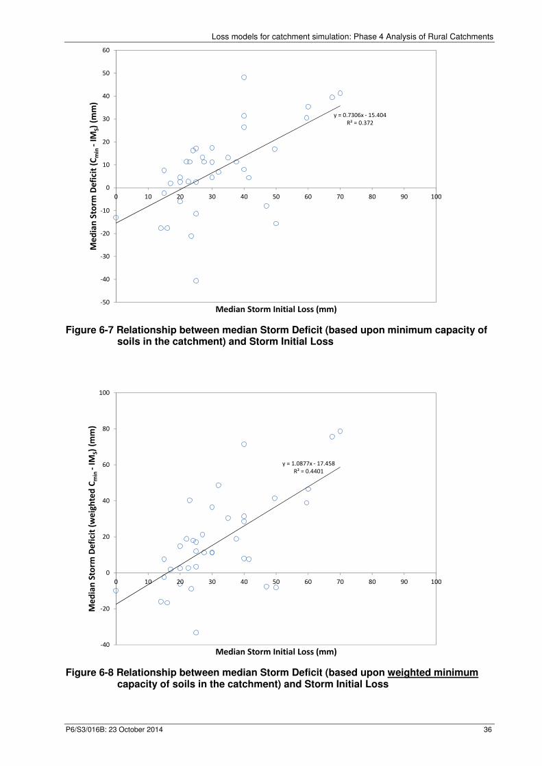
Loss models for catchment simulation: Phase 4 Analysis of Rural Catchments
P6/S3/016B: 23 October 2014 36
Figure 6-7 Relationship between median Storm Deficit (based upon minimum capacity of soils in the catchment) and Storm Initial Loss
Figure 6-8 Relationship between median Storm Deficit (based upon weighted minimum
capacity of soils in the catchment) and Storm Initial Loss
y = 0.7306x - 15.404
R² = 0.372
-50
-40
-30
-20
-10
0
10
20
30
40
50
60
0 10 20 30 40 50 60 70 80 90 100
Me
dia
n S
torm
De
fici
t (C
min
-IM
S)
(mm
)
Median Storm Initial Loss (mm)
y = 1.0877x - 17.458
R² = 0.4401
-40
-20
0
20
40
60
80
100
0 10 20 30 40 50 60 70 80 90 100
Me
dia
n S
torm
De
fici
t (w
eig
hte
d C
min
-IM
S)
(mm
)
Median Storm Initial Loss (mm)
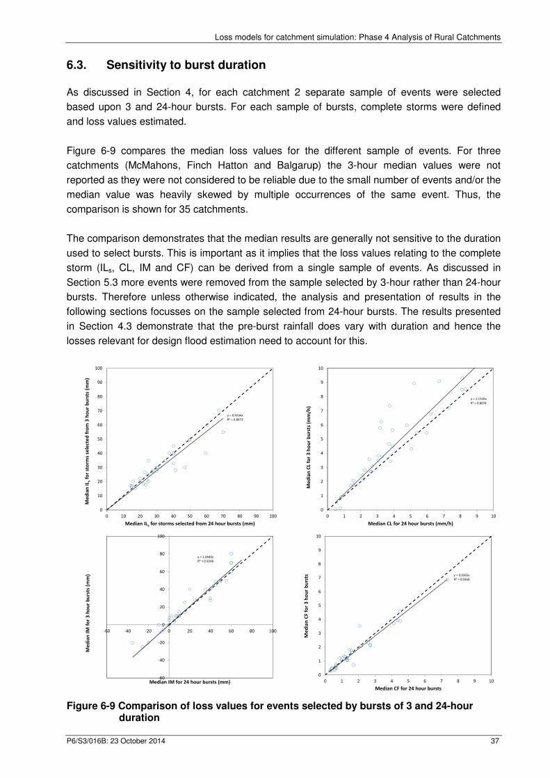
Loss models for catchment simulation: Phase 4 Analysis of Rural Catchments
P6/S3/016B: 23 October 2014 37
6.3. Sensitivity to burst duration
As discussed in Section 4, for each catchment 2 separate sample of events were selected
based upon 3 and 24-hour bursts. For each sample of bursts, complete storms were defined
and loss values estimated.
Figure 6-9 compares the median loss values for the different sample of events. For three
catchments (McMahons, Finch Hatton and Balgarup) the 3-hour median values were not
reported as they were not considered to be reliable due to the small number of events and/or the
median value was heavily skewed by multiple occurrences of the same event. Thus, the
comparison is shown for 35 catchments.
The comparison demonstrates that the median results are generally not sensitive to the duration
used to select bursts. This is important as it implies that the loss values relating to the complete
storm (ILs, CL, IM and CF) can be derived from a single sample of events. As discussed in
Section 5.3 more events were removed from the sample selected by 3-hour rather than 24-hour
bursts. Therefore unless otherwise indicated, the analysis and presentation of results in the
following sections focusses on the sample selected from 24-hour bursts. The results presented
in Section 4.3 demonstrate that the pre-burst rainfall does vary with duration and hence the
losses relevant for design flood estimation need to account for this.
Figure 6-9 Comparison of loss values for events selected by bursts of 3 and 24-hour
duration
y = 0.9234x
R² = 0.8372
0
10
20
30
40
50
60
70
80
90
100
0 10 20 30 40 50 60 70 80 90 100
Me
dia
n I
L sfo
r st
orm
s se
lect
ed
fro
m 3
ho
ur
bu
rsts
(m
m)
Median ILs for storms selected from 24 hour bursts (mm)
y = 1.1316x
R² = 0.8074
0
1
2
3
4
5
6
7
8
9
10
0 1 2 3 4 5 6 7 8 9 10
Me
dia
n C
L fo
r 3
ho
ur
bu
rsts
(m
m/h
)
Median CL for 24 hour bursts (mm/h)
y = 1.0446x
R² = 0.9248
-60
-40
-20
0
20
40
60
80
100
-60 -40 -20 0 20 40 60 80 100
Me
dia
n I
M f
or
3 h
ou
r b
urs
ts (
mm
)
Median IM for 24 hour bursts (mm)
y = 0.9365x
R² = 0.9366
0
1
2
3
4
5
6
7
8
9
10
0 1 2 3 4 5 6 7 8 9 10
Me
dia
n C
F f
or
3 h
ou
r b
urs
ts
Median CF for 24 hour bursts
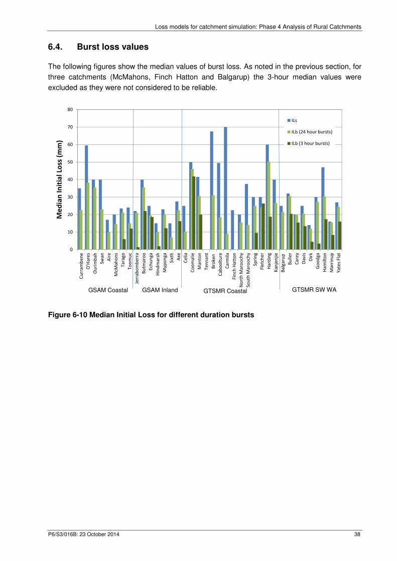
Loss models for catchment simulation: Phase 4 Analysis of Rural Catchments
P6/S3/016B: 23 October 2014 38
6.4. Burst loss values
The following figures show the median values of burst loss. As noted in the previous section, for
three catchments (McMahons, Finch Hatton and Balgarup) the 3-hour median values were
excluded as they were not considered to be reliable.
Figure 6-10 Median Initial Loss for different duration bursts
0
10
20
30
40
50
60
70
80
Cu
rra
mb
en
e
O'H
are
s
Ou
rim
ba
h
Swa
n
Air
e
McM
ah
on
s
Ta
rag
o
To
om
uc
Jerr
ab
om
be
rra
Bu
tma
roo
Ech
un
ga
Hin
dm
ars
h
Myp
on
ga
Sixt
h
Axe
Ce
lia
Co
om
ali
e
Ma
nto
n
Te
nn
an
t
Bro
ken
Ca
bo
olt
ure
Ca
rmil
a
Fin
ch H
att
on
No
rth
Ma
roo
chy
So
uth
Ma
roo
chy
Spri
ng
Fle
tch
er
Ha
rdin
g
Ka
nje
nji
e
Ba
lga
rup
Bu
ller
Ca
rey
Da
vis
Dir
k
Go
od
ga
Ha
mil
ton
Ma
rrin
up
Ya
tes
Fla
t
Me
dia
n I
nit
ial
Loss
(m
m)
ILs
ILb (24 hour bursts)
ILb (3 hour bursts)
GSAM Coastal GSAM Inland GTSMR Coastal GTSMR SW WA
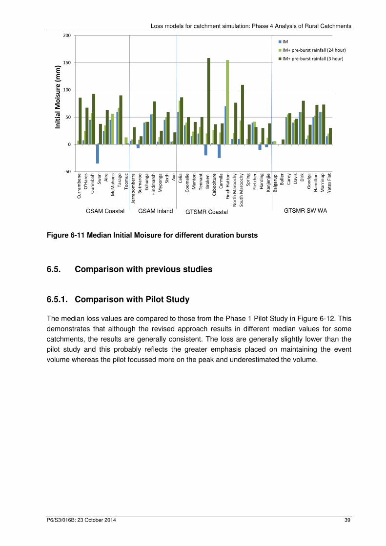
Loss models for catchment simulation: Phase 4 Analysis of Rural Catchments
P6/S3/016B: 23 October 2014 39
Figure 6-11 Median Initial Moisure for different duration bursts
6.5. Comparison with previous studies
6.5.1. Comparison with Pilot Study
The median loss values are compared to those from the Phase 1 Pilot Study in Figure 6-12. This
demonstrates that although the revised approach results in different median values for some
catchments, the results are generally consistent. The loss are generally slightly lower than the
pilot study and this probably reflects the greater emphasis placed on maintaining the event
volume whereas the pilot focussed more on the peak and underestimated the volume.
-50
0
50
100
150
200
Cu
rra
mb
en
e
O'H
are
s
Ou
rim
ba
h
Sw
an
Air
e
McM
ah
on
s
Ta
rag
o
To
om
uc
Jerr
ab
om
be
rra
Bu
tma
roo
Ech
un
ga
Hin
dm
ars
h
Myp
on
ga
Sixt
h
Axe
Ce
lia
Co
om
alie
Ma
nto
n
Te
nn
an
t
Bro
ken
Ca
bo
olt
ure
Ca
rmila
Fin
ch H
att
on
No
rth
Ma
roo
chy
Sou
th M
aro
och
y
Spri
ng
Fle
tch
er
Ha
rdin
g
Ka
nje
nji
e
Ba
lga
rup
Bu
lle
r
Ca
rey
Da
vis
Dir
k
Go
od
ga
Ha
milt
on
Ma
rrin
up
Ya
tes
Fla
t
Init
ial
Mo
isu
re (
mm
)
IM
IM+ pre-burst rainfall (24 hour)
IM+ pre-burst rainfall (3 hour)
GSAM Coastal GSAM Inland GTSMR Coastal GTSMR SW WA
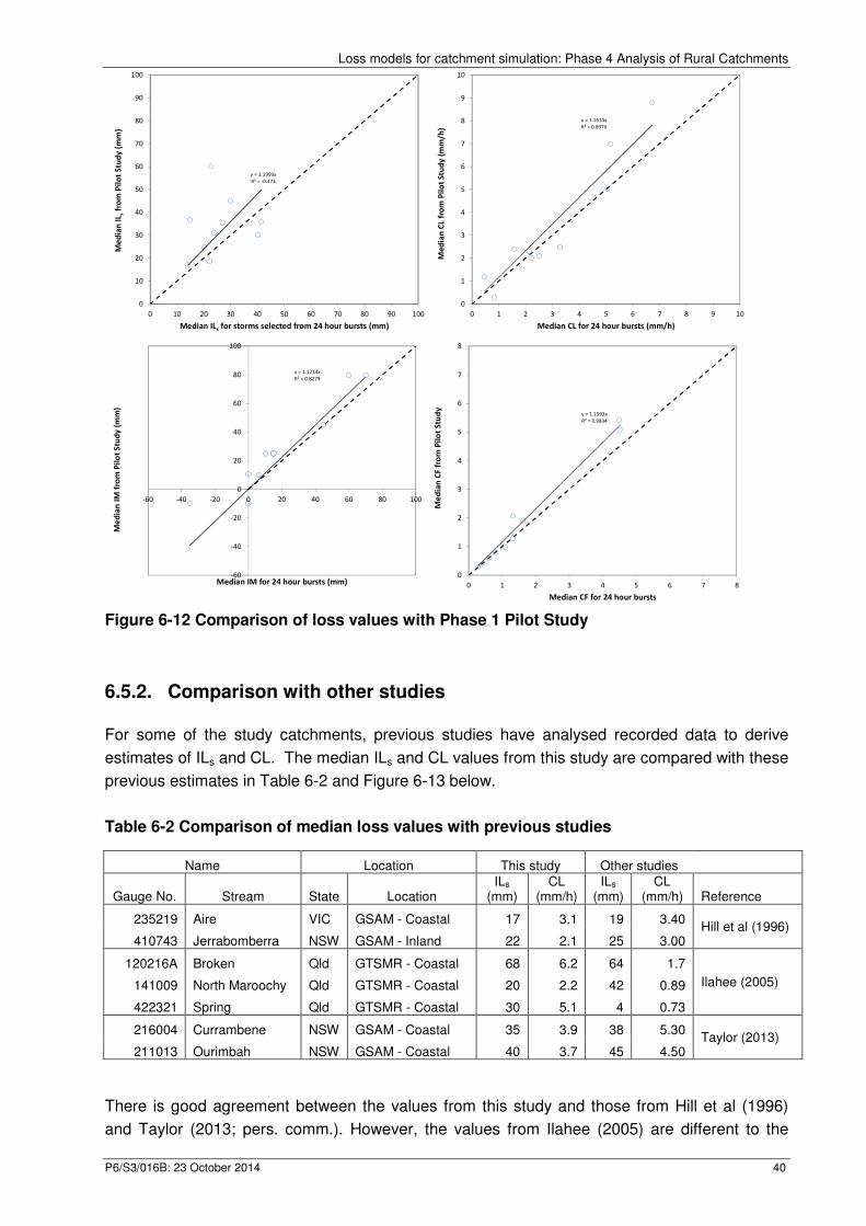
Loss models for catchment simulation: Phase 4 Analysis of Rural Catchments
P6/S3/016B: 23 October 2014 40
Figure 6-12 Comparison of loss values with Phase 1 Pilot Study
6.5.2. Comparison with other studies
For some of the study catchments, previous studies have analysed recorded data to derive
estimates of ILs and CL. The median ILs and CL values from this study are compared with these
previous estimates in Table 6-2 and Figure 6-13 below.
Table 6-2 Comparison of median loss values with previous studies
Name Location This study Other studies
Gauge No. Stream State Location ILs
(mm) CL
(mm/h) ILs
(mm) CL
(mm/h) Reference
235219 Aire VIC GSAM - Coastal 17 3.1 19 3.40 Hill et al (1996)
410743 Jerrabomberra NSW GSAM - Inland 22 2.1 25 3.00
120216A Broken Qld GTSMR - Coastal 68 6.2 64 1.7
Ilahee (2005) 141009 North Maroochy Qld GTSMR - Coastal 20 2.2 42 0.89
422321 Spring Qld GTSMR - Coastal 30 5.1 4 0.73
216004 Currambene NSW GSAM - Coastal 35 3.9 38 5.30 Taylor (2013)
211013 Ourimbah NSW GSAM - Coastal 40 3.7 45 4.50
There is good agreement between the values from this study and those from Hill et al (1996)
and Taylor (2013; pers. comm.). However, the values from Ilahee (2005) are different to the
y = 1.1993x
R² = -0.473
0
10
20
30
40
50
60
70
80
90
100
0 10 20 30 40 50 60 70 80 90 100
Me
dia
n I
L sfr
om
Pil
ot
Stu
dy
(m
m)
Median ILs for storms selected from 24 hour bursts (mm)
y = 1.1614x
R² = 0.8976
0
1
2
3
4
5
6
7
8
9
10
0 1 2 3 4 5 6 7 8 9 10
Me
dia
n C
L fr
om
Pil
ot
Stu
dy
(m
m/h
)
Median CL for 24 hour bursts (mm/h)
y = 1.1214x
R² = 0.8279
-60
-40
-20
0
20
40
60
80
100
-60 -40 -20 0 20 40 60 80 100
Me
dia
n I
M f
rom
Pil
ot
Stu
dy
(m
m)
Median IM for 24 hour bursts (mm)
y = 1.1593x
R² = 0.9834
0
1
2
3
4
5
6
7
8
0 1 2 3 4 5 6 7 8
Me
dia
n C
F fr
om
Pil
ot
Stu
dy
Median CF for 24 hour bursts
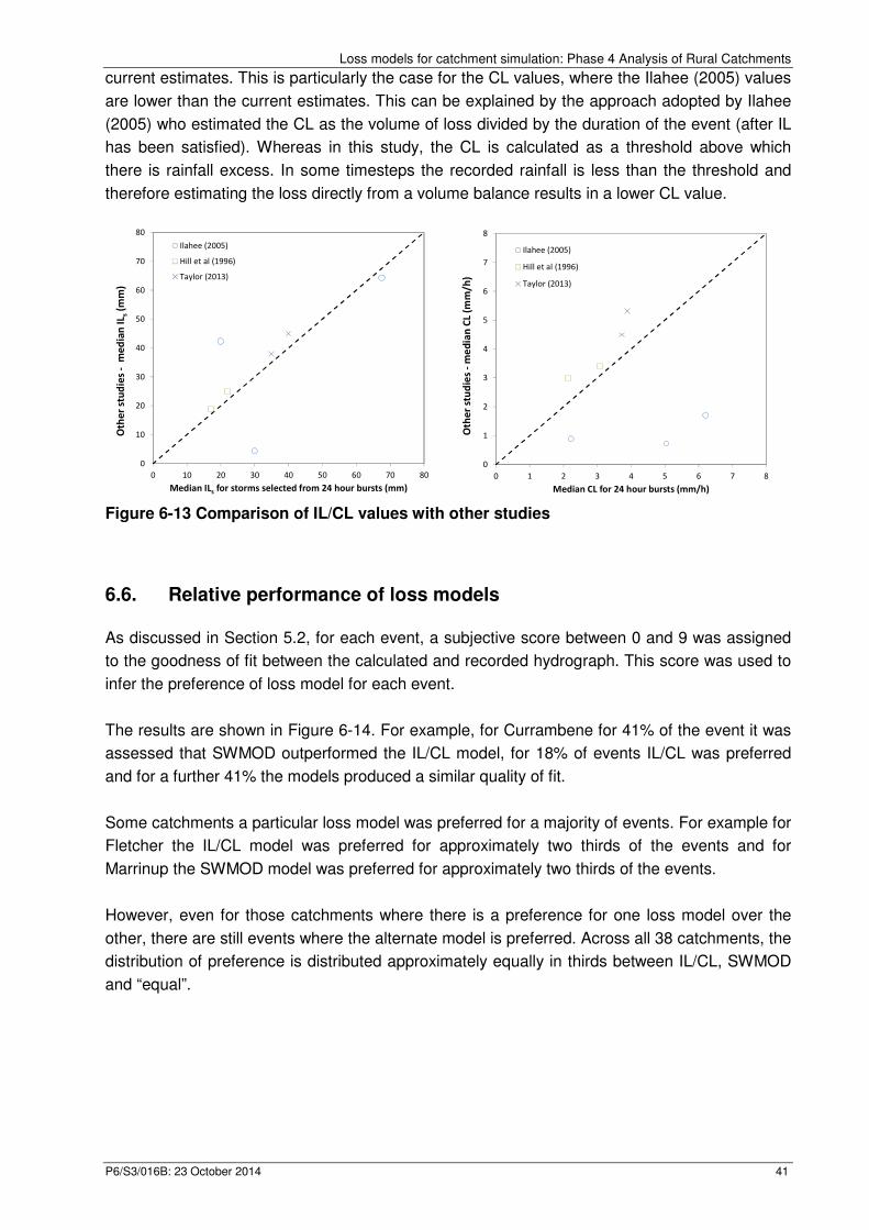
Loss models for catchment simulation: Phase 4 Analysis of Rural Catchments
P6/S3/016B: 23 October 2014 41
current estimates. This is particularly the case for the CL values, where the Ilahee (2005) values
are lower than the current estimates. This can be explained by the approach adopted by Ilahee
(2005) who estimated the CL as the volume of loss divided by the duration of the event (after IL
has been satisfied). Whereas in this study, the CL is calculated as a threshold above which
there is rainfall excess. In some timesteps the recorded rainfall is less than the threshold and
therefore estimating the loss directly from a volume balance results in a lower CL value.
Figure 6-13 Comparison of IL/CL values with other studies
6.6. Relative performance of loss models
As discussed in Section 5.2, for each event, a subjective score between 0 and 9 was assigned
to the goodness of fit between the calculated and recorded hydrograph. This score was used to
infer the preference of loss model for each event.
The results are shown in Figure 6-14. For example, for Currambene for 41% of the event it was
assessed that SWMOD outperformed the IL/CL model, for 18% of events IL/CL was preferred
and for a further 41% the models produced a similar quality of fit.
Some catchments a particular loss model was preferred for a majority of events. For example for
Fletcher the IL/CL model was preferred for approximately two thirds of the events and for
Marrinup the SWMOD model was preferred for approximately two thirds of the events.
However, even for those catchments where there is a preference for one loss model over the
other, there are still events where the alternate model is preferred. Across all 38 catchments, the
distribution of preference is distributed approximately equally in thirds between IL/CL, SWMOD
and “equal”.
0
10
20
30
40
50
60
70
80
0 10 20 30 40 50 60 70 80
Oth
er
stu
die
s -
me
dia
n I
L s(m
m)
Median ILs for storms selected from 24 hour bursts (mm)
Ilahee (2005)
Hill et al (1996)
Taylor (2013)
0
1
2
3
4
5
6
7
8
0 1 2 3 4 5 6 7 8O
the
r st
ud
ies
-m
ed
ian
CL
(mm
/h)
Median CL for 24 hour bursts (mm/h)
Ilahee (2005)
Hill et al (1996)
Taylor (2013)
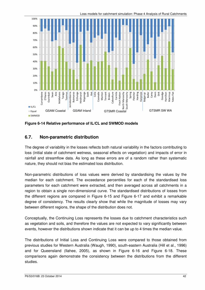
Loss models for catchment simulation: Phase 4 Analysis of Rural Catchments
P6/S3/016B: 23 October 2014 42
Figure 6-14 Relative performance of IL/CL and SWMOD models
6.7. Non-parametric distribution
The degree of variability in the losses reflects both natural variability in the factors contributing to
loss (initial state of catchment wetness, seasonal effects on vegetation) and impacts of error in
rainfall and streamflow data. As long as these errors are of a random rather than systematic
nature, they should not bias the estimated loss distribution.
Non-parametric distributions of loss values were derived by standardising the values by the
median for each catchment. The exceedance percentiles for each of the standardised loss
parameters for each catchment were extracted, and then averaged across all catchments in a
region to obtain a single non-dimensional curve. The standardised distributions of losses from
the different regions are compared in Figure 6-15 and Figure 6-17 and exhibit a remarkable
degree of consistency. The results clearly show that while the magnitude of losses may vary
between different regions, the shape of the distribution does not.
Conceptually, the Continuing Loss represents the losses due to catchment characteristics such
as vegetation and soils, and therefore the values are not expected to vary significantly between
events, however the distributions shown indicate that it can be up to 4 times the median value.
The distributions of Initial Loss and Continuing Loss were compared to those obtained from
previous studies for Western Australia (Waugh, 1990), south-eastern Australia (Hill et al., 1996)
and for Queensland (Ilahee, 2005), as shown in Figure 6-16 and Figure 6-18. These
comparisons again demonstrate the consistency between the distributions from the different
studies.
0%
10%
20%
30%
40%
50%
60%
70%
80%
90%
100%
Cu
rra
mb
en
e
O'H
are
s
Ou
rim
ba
h
Sw
an
Air
e
McM
ah
on
s
Ta
rag
o
To
om
uc
Jerr
ab
om
be
rra
Bu
tma
roo
Ech
un
ga
Hin
dm
ars
h
Myp
on
ga
Six
th
Axe
Ce
lia
Co
om
alie
Ma
nto
n
Te
nn
an
t
Bro
ken
Ca
bo
olt
ure
Ca
rmila
Fin
ch H
att
on
No
rth
Ma
roo
chy
So
uth
Ma
roo
chy
Sp
rin
g
Fle
tch
er
Ha
rdin
g
Ka
nje
nji
e
Ba
lga
rup
Bu
ller
Ca
rey
Da
vis
Dir
k
Go
od
ga
Ha
milt
on
Ma
rrin
up
Ya
tes
Fla
t
IL/CL
Equal
SWMOD
GSAM Coastal GSAM Inland GTSMR Coastal GTSMR SW WA
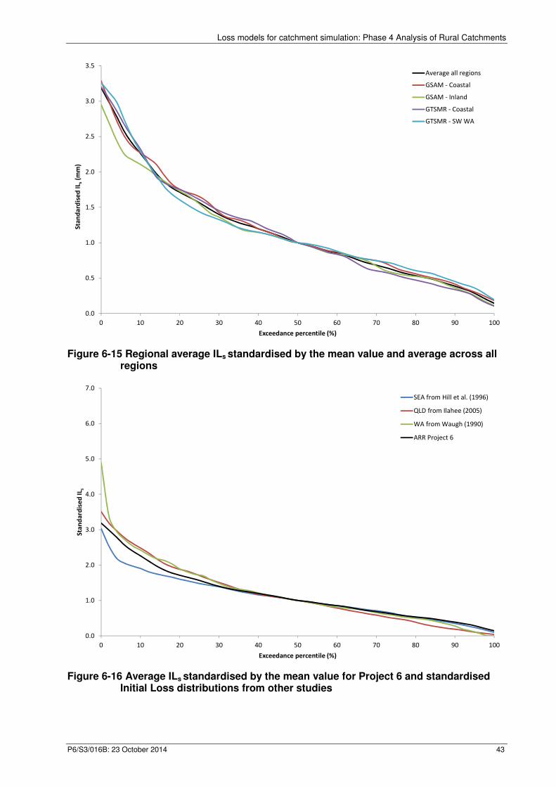
Loss models for catchment simulation: Phase 4 Analysis of Rural Catchments
P6/S3/016B: 23 October 2014 43
Figure 6-15 Regional average ILs standardised by the mean value and average across all regions
Figure 6-16 Average ILs standardised by the mean value for Project 6 and standardised Initial Loss distributions from other studies
0.0
0.5
1.0
1.5
2.0
2.5
3.0
3.5
0 10 20 30 40 50 60 70 80 90 100
Sta
nd
ard
ise
d I
L s(m
m)
Exceedance percentile (%)
Average all regions
GSAM - Coastal
GSAM - Inland
GTSMR - Coastal
GTSMR - SW WA
0.0
1.0
2.0
3.0
4.0
5.0
6.0
7.0
0 10 20 30 40 50 60 70 80 90 100
Sta
nd
ard
ise
d I
L s
Exceedance percentile (%)
SEA from Hill et al. (1996)
QLD from Ilahee (2005)
WA from Waugh (1990)
ARR Project 6
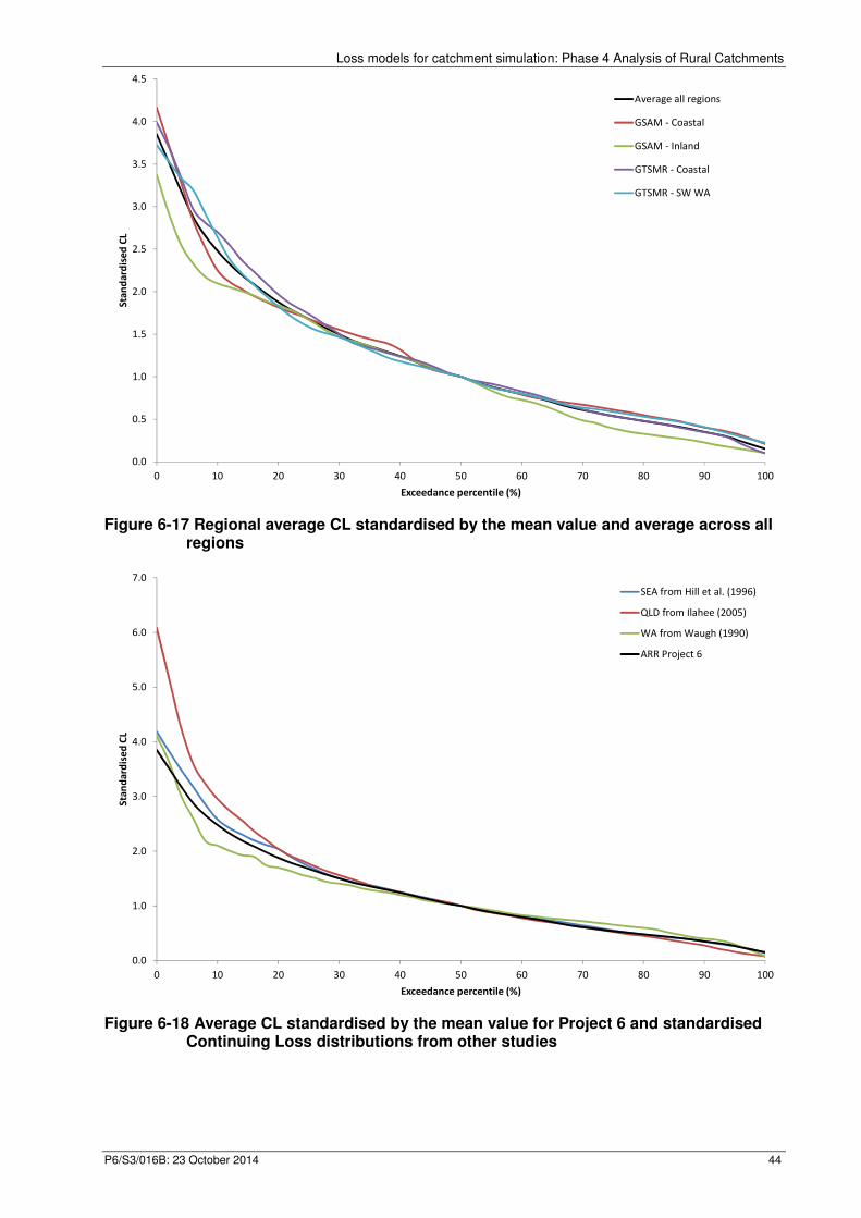
Loss models for catchment simulation: Phase 4 Analysis of Rural Catchments
P6/S3/016B: 23 October 2014 44
Figure 6-17 Regional average CL standardised by the mean value and average across all regions
Figure 6-18 Average CL standardised by the mean value for Project 6 and standardised Continuing Loss distributions from other studies
0.0
0.5
1.0
1.5
2.0
2.5
3.0
3.5
4.0
4.5
0 10 20 30 40 50 60 70 80 90 100
Sta
nd
ard
ise
d C
L
Exceedance percentile (%)
Average all regions
GSAM - Coastal
GSAM - Inland
GTSMR - Coastal
GTSMR - SW WA
0.0
1.0
2.0
3.0
4.0
5.0
6.0
7.0
0 10 20 30 40 50 60 70 80 90 100
Sta
nd
ard
ise
d C
L
Exceedance percentile (%)
SEA from Hill et al. (1996)
QLD from Ilahee (2005)
WA from Waugh (1990)
ARR Project 6
Loss models for catchment simulation: Phase 4 Analysis of Rural Catchments
P6/S3/016B: 23 October 2014 45
6.8. Relationship with antecedent conditions
The antecedent precipitation index (API) is a measure of the initial wetness of a catchment. API
is calculated by discounting the time series of daily rainfall prior to the event using an empirical
decay factor and the basic equations is (Cordery, 1970):
APId = Pd + k.Pd-1+ k2.Pd-2 + …
Where k is an empirical decay factor less than unity and Pd is rainfall for day d. The value of k
varies typically in the range of 0.85 to 0.98 (Linsley et al., 1982) and Cordery (1970) found that
the average relationship for Australian catchments was 0.92. The value of k is considered to
vary seasonally and has been linked to the variation in potential evapotranspiration (Mein et al.
1995).
For this study a fixed k was adopted throughout the year and values of 0.85, 0.90 and 0.95 were
trialled. The relationship between the API and the ILs and IMs was explored by simple linear
regression and the r2 are summarised in Figure 6-19 and Figure 6-20. For both the ILs and IMs
the highest correlation was obtained with a k of 0.95 and hence this was adopted consistently
across all catchments.
For some catchments the API explains a large proportion of the variance in ILs and IMs whereas
for other catchments the loss values appear to be invariant with API. This would indicate that the
variability of losses is driven by factors other than antecedent rainfall and it is recommended that
this be further investigated.
The ranges of values of API for each catchment are shown in Figure 6-21 for a k of 0.95 for
storms selected based upon 24-hour bursts. The range of API values for the sample of events
based upon different duration bursts is shown in Appendix E. The API values are not sensitive to
the burst duration used to select the events and this is consistent with the findings for ILs and IMs
noted above.
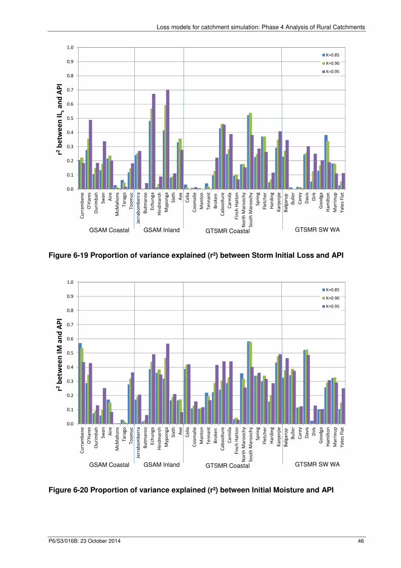
Loss models for catchment simulation: Phase 4 Analysis of Rural Catchments
P6/S3/016B: 23 October 2014 46
Figure 6-19 Proportion of variance explained (r²) between Storm Initial Loss and API
Figure 6-20 Proportion of variance explained (r²) between Initial Moisture and API
0.0
0.1
0.2
0.3
0.4
0.5
0.6
0.7
0.8
0.9
1.0
Cu
rra
mb
en
e
O'H
are
s
Ou
rim
ba
h
Swa
n
Air
e
McM
ah
on
s
Ta
rag
o
To
om
uc
Jerr
ab
om
be
rra
Bu
tma
roo
Ech
un
ga
Hin
dm
ars
h
Myp
on
ga
Six
th
Axe
Ce
lia
Co
om
ali
e
Ma
nto
n
Te
nn
an
t
Bro
ken
Ca
bo
olt
ure
Ca
rmila
Fin
ch H
att
on
No
rth
Ma
roo
chy
Sou
th M
aro
och
y
Sp
rin
g
Fle
tch
er
Ha
rdin
g
Ka
nje
nji
e
Ba
lga
rup
Bu
ller
Ca
rey
Da
vis
Dir
k
Go
od
ga
Ha
milt
on
Ma
rrin
up
Ya
tes
Fla
t
r2b
etw
ee
n I
L sa
nd
AP
IK=0.85
K=0.90
K=0.95
GSAM Coastal GSAM Inland GTSMR Coastal GTSMR SW WA
0.0
0.1
0.2
0.3
0.4
0.5
0.6
0.7
0.8
0.9
1.0
Cu
rra
mb
en
e
O'H
are
s
Ou
rim
ba
h
Sw
an
Air
e
McM
ah
on
s
Ta
rag
o
To
om
uc
Jerr
ab
om
be
rra
Bu
tma
roo
Ech
un
ga
Hin
dm
ars
h
Myp
on
ga
Sixt
h
Axe
Ce
lia
Co
om
alie
Ma
nto
n
Te
nn
an
t
Bro
ken
Ca
bo
olt
ure
Ca
rmila
Fin
ch H
att
on
No
rth
Ma
roo
chy
Sou
th M
aro
och
y
Spri
ng
Fle
tch
er
Ha
rdin
g
Ka
nje
nji
e
Ba
lga
rup
Bu
lle
r
Ca
rey
Da
vis
Dir
k
Go
od
ga
Ha
milt
on
Ma
rrin
up
Ya
tes
Fla
t
r2b
etw
ee
n I
M a
nd
AP
I
K=0.85
K=0.90
K=0.95
GSAM Coastal GSAM Inland GTSMR Coastal GTSMR SW WA
P6/S3/016B: 23 October 2014
Figure 6-21 Range of API values (box indicates quartiles and line shows
6.9. Variation with storm
The catchment specific loss s
values versus the storm severity which is characterised as the average recurrence (ARI) of the
rainfall burst. It is difficult to infer the variation of loss values with storm severity because
lack of severe rainfalls recorded for a particular catchment. It should be noted however, that the
storm severity is characterised as the ARI of the rainfall burst whereas the loss values relate to
the complete storm and this discrepancy further hi
severity.
The events for all catchments were therefore pooled by standardising by the median values. The
variation of standardised loss with ARI is presented in the following figures and shows that there
is no systematic variation of loss values with ARI. This is consistent with a range of previous
studies that have failed to find a trend with ARI.
Loss models for catchment simulation: Phase 4 Analysis of Rural Catchments
values (k=0.95) for storm selected by 24-hour(box indicates quartiles and line shows 10th and 90th percentile
torm severity
The catchment specific loss summaries provided in Appendix I and J include plots of the loss
values versus the storm severity which is characterised as the average recurrence (ARI) of the
rainfall burst. It is difficult to infer the variation of loss values with storm severity because
lack of severe rainfalls recorded for a particular catchment. It should be noted however, that the
storm severity is characterised as the ARI of the rainfall burst whereas the loss values relate to
the complete storm and this discrepancy further hinders the identification of any trend with storm
The events for all catchments were therefore pooled by standardising by the median values. The
variation of standardised loss with ARI is presented in the following figures and shows that there
no systematic variation of loss values with ARI. This is consistent with a range of previous
studies that have failed to find a trend with ARI.
Loss models for catchment simulation: Phase 4 Analysis of Rural Catchments
47
hour bursts percentile values)
include plots of the loss
values versus the storm severity which is characterised as the average recurrence (ARI) of the
rainfall burst. It is difficult to infer the variation of loss values with storm severity because of the
lack of severe rainfalls recorded for a particular catchment. It should be noted however, that the
storm severity is characterised as the ARI of the rainfall burst whereas the loss values relate to
nders the identification of any trend with storm
The events for all catchments were therefore pooled by standardising by the median values. The
variation of standardised loss with ARI is presented in the following figures and shows that there
no systematic variation of loss values with ARI. This is consistent with a range of previous
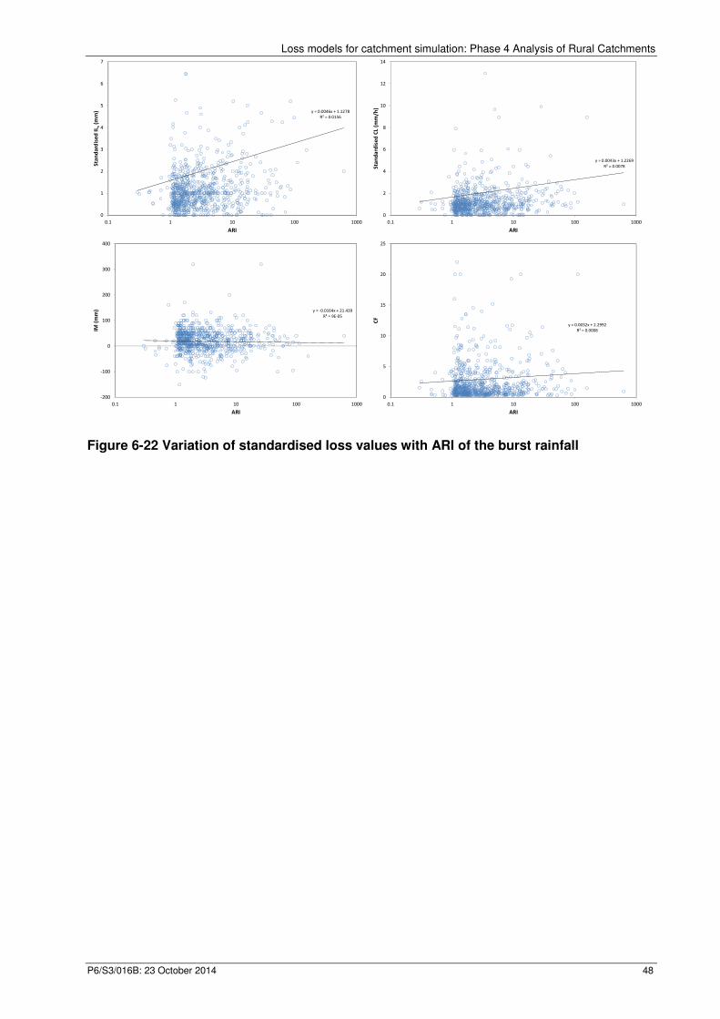
Loss models for catchment simulation: Phase 4 Analysis of Rural Catchments
P6/S3/016B: 23 October 2014 48
Figure 6-22 Variation of standardised loss values with ARI of the burst rainfall
y = 0.0046x + 1.1278
R² = 0.0156
0
1
2
3
4
5
6
7
0.1 1 10 100 1000
Sta
nd
ard
ise
d I
L s(m
m)
ARI
y = 0.0043x + 1.2269
R² = 0.0078
0
2
4
6
8
10
12
14
0.1 1 10 100 1000
Sta
nd
ard
ise
d C
L (m
m/h
)
ARI
y = -0.0164x + 21.439
R² = 9E-05
-200
-100
0
100
200
300
400
0.1 1 10 100 1000
IM (
mm
)
ARI
y = 0.0032x + 2.2992
R² = 0.0008
0
5
10
15
20
25
0.1 1 10 100 1000
CF
ARI
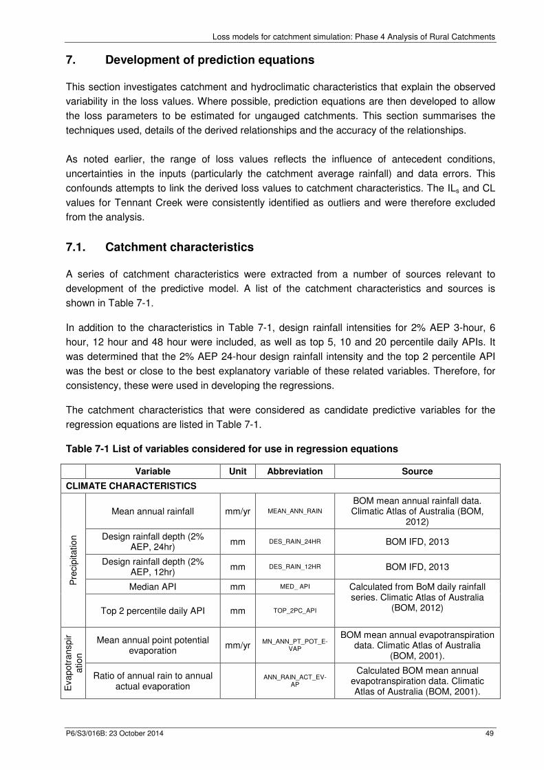
Loss models for catchment simulation: Phase 4 Analysis of Rural Catchments
P6/S3/016B: 23 October 2014 49
7. Development of prediction equations
This section investigates catchment and hydroclimatic characteristics that explain the observed
variability in the loss values. Where possible, prediction equations are then developed to allow
the loss parameters to be estimated for ungauged catchments. This section summarises the
techniques used, details of the derived relationships and the accuracy of the relationships.
As noted earlier, the range of loss values reflects the influence of antecedent conditions,
uncertainties in the inputs (particularly the catchment average rainfall) and data errors. This
confounds attempts to link the derived loss values to catchment characteristics. The ILs and CL
values for Tennant Creek were consistently identified as outliers and were therefore excluded
from the analysis.
7.1. Catchment characteristics
A series of catchment characteristics were extracted from a number of sources relevant to
development of the predictive model. A list of the catchment characteristics and sources is
shown in Table 7-1.
In addition to the characteristics in Table 7-1, design rainfall intensities for 2% AEP 3-hour, 6
hour, 12 hour and 48 hour were included, as well as top 5, 10 and 20 percentile daily APIs. It
was determined that the 2% AEP 24-hour design rainfall intensity and the top 2 percentile API
was the best or close to the best explanatory variable of these related variables. Therefore, for
consistency, these were used in developing the regressions.
The catchment characteristics that were considered as candidate predictive variables for the
regression equations are listed in Table 7-1.
Table 7-1 List of variables considered for use in regression equations
Variable Unit Abbreviation Source
CLIMATE CHARACTERISTICS
Pre
cip
itatio
n
Mean annual rainfall mm/yr MEAN_ANN_RAIN
BOM mean annual rainfall data. Climatic Atlas of Australia (BOM,
2012)
Design rainfall depth (2% AEP, 24hr)
mm DES_RAIN_24HR BOM IFD, 2013
Design rainfall depth (2% AEP, 12hr)
mm DES_RAIN_12HR BOM IFD, 2013
Median API mm MED_ API Calculated from BoM daily rainfall series. Climatic Atlas of Australia
(BOM, 2012)
Top 2 percentile daily API mm TOP_2PC_API
Evapotr
anspir
atio
n
Mean annual point potential evaporation
mm/yr MN_ANN_PT_POT_E-
VAP
BOM mean annual evapotranspiration data. Climatic Atlas of Australia
(BOM, 2001).
Ratio of annual rain to annual actual evaporation
ANN_RAIN_ACT_EV-
AP
Calculated BOM mean annual evapotranspiration data. Climatic Atlas of Australia (BOM, 2001).
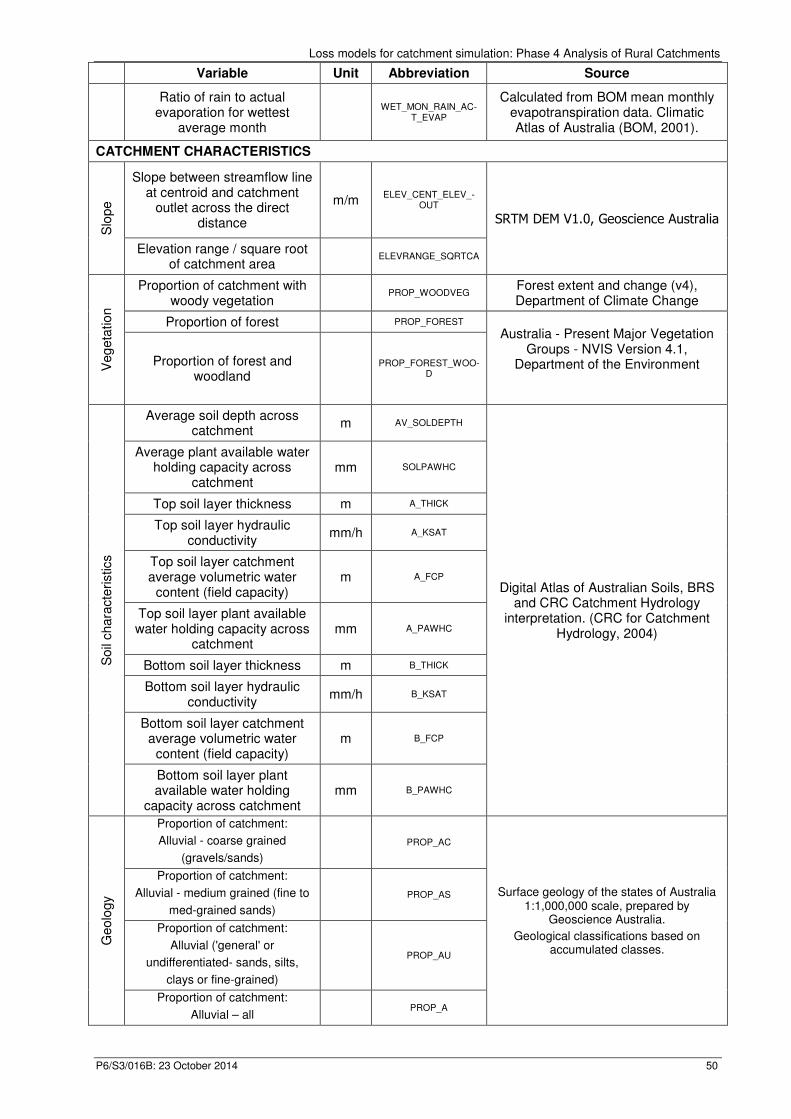
Loss models for catchment simulation: Phase 4 Analysis of Rural Catchments
P6/S3/016B: 23 October 2014 50
Variable Unit Abbreviation Source
Ratio of rain to actual evaporation for wettest
average month
WET_MON_RAIN_AC- T_EVAP
Calculated from BOM mean monthly evapotranspiration data. Climatic Atlas of Australia (BOM, 2001).
CATCHMENT CHARACTERISTICS
Slo
pe
Slope between streamflow line at centroid and catchment
outlet across the direct distance
m/m ELEV_CENT_ELEV_-
OUT
SRTM DEM V1.0, Geoscience Australia
Elevation range / square root of catchment area
ELEVRANGE_SQRTCA
Veg
eta
tio
n
Proportion of catchment with woody vegetation
PROP_WOODVEG Forest extent and change (v4), Department of Climate Change
Proportion of forest PROP_FOREST
Australia - Present Major Vegetation Groups - NVIS Version 4.1,
Department of the Environment
Proportion of forest and woodland
PROP_FOREST_WOO-
D
Soil
chara
cte
ristics
Average soil depth across catchment
m AV_SOLDEPTH
Digital Atlas of Australian Soils, BRS and CRC Catchment Hydrology
interpretation. (CRC for Catchment Hydrology, 2004)
Average plant available water holding capacity across
catchment mm SOLPAWHC
Top soil layer thickness m A_THICK
Top soil layer hydraulic conductivity
mm/h A_KSAT
Top soil layer catchment average volumetric water
content (field capacity) m A_FCP
Top soil layer plant available water holding capacity across
catchment mm A_PAWHC
Bottom soil layer thickness m B_THICK
Bottom soil layer hydraulic conductivity
mm/h B_KSAT
Bottom soil layer catchment average volumetric water
content (field capacity) m B_FCP
Bottom soil layer plant available water holding
capacity across catchment mm B_PAWHC
Geolo
gy
Proportion of catchment:
Alluvial - coarse grained
(gravels/sands)
PROP_AC
Surface geology of the states of Australia 1:1,000,000 scale, prepared by
Geoscience Australia.
Geological classifications based on accumulated classes.
Proportion of catchment:
Alluvial - medium grained (fine to
med-grained sands)
PROP_AS
Proportion of catchment:
Alluvial ('general' or
undifferentiated- sands, silts,
clays or fine-grained)
PROP_AU
Proportion of catchment:
Alluvial – all PROP_A
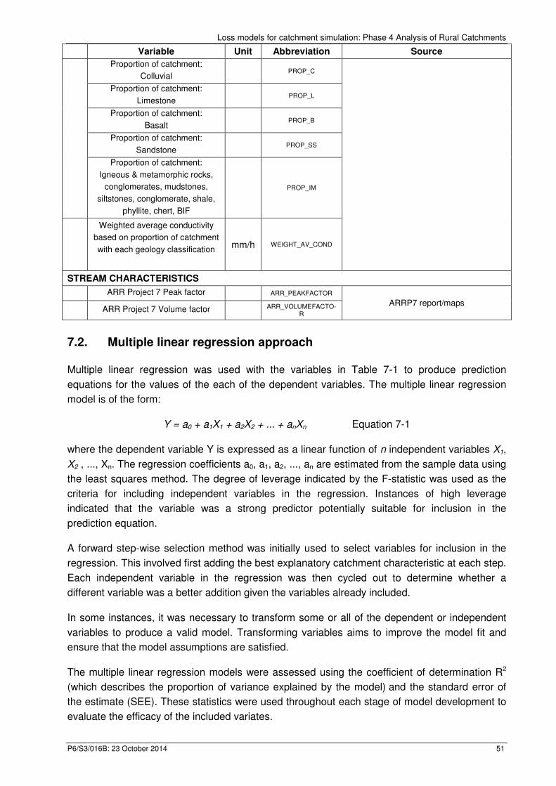
Loss models for catchment simulation: Phase 4 Analysis of Rural Catchments
P6/S3/016B: 23 October 2014 51
Variable Unit Abbreviation Source
Proportion of catchment:
Colluvial PROP_C
Proportion of catchment:
Limestone PROP_L
Proportion of catchment:
Basalt PROP_B
Proportion of catchment:
Sandstone PROP_SS
Proportion of catchment:
Igneous & metamorphic rocks,
conglomerates, mudstones,
siltstones, conglomerate, shale,
phyllite, chert, BIF
PROP_IM
Weighted average conductivity
based on proportion of catchment
with each geology classification
mm/h WEIGHT_AV_COND
STREAM CHARACTERISTICS
ARR Project 7 Peak factor ARR_PEAKFACTOR
ARRP7 report/maps ARR Project 7 Volume factor
ARR_VOLUMEFACTO- R
7.2. Multiple linear regression approach
Multiple linear regression was used with the variables in Table 7-1 to produce prediction
equations for the values of the each of the dependent variables. The multiple linear regression
model is of the form:
Y = a0 + a1X1 + a2X2 + ... + anXn Equation 7-1
where the dependent variable Y is expressed as a linear function of n independent variables X1,
X2 , ..., Xn. The regression coefficients a0, a1, a2, ..., an are estimated from the sample data using
the least squares method. The degree of leverage indicated by the F-statistic was used as the
criteria for including independent variables in the regression. Instances of high leverage
indicated that the variable was a strong predictor potentially suitable for inclusion in the
prediction equation.
A forward step-wise selection method was initially used to select variables for inclusion in the
regression. This involved first adding the best explanatory catchment characteristic at each step.
Each independent variable in the regression was then cycled out to determine whether a
different variable was a better addition given the variables already included.
In some instances, it was necessary to transform some or all of the dependent or independent
variables to produce a valid model. Transforming variables aims to improve the model fit and
ensure that the model assumptions are satisfied.
The multiple linear regression models were assessed using the coefficient of determination R2
(which describes the proportion of variance explained by the model) and the standard error of
the estimate (SEE). These statistics were used throughout each stage of model development to
evaluate the efficacy of the included variates.
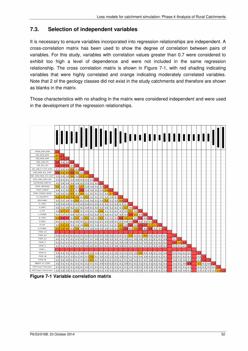
Loss models for catchment simulation: Phase 4 Analysis of Rural Catchments
P6/S3/016B: 23 October 2014 52
7.3. Selection of independent variables
It is necessary to ensure variables incorporated into regression relationships are independent. A
cross-correlation matrix has been used to show the degree of correlation between pairs of
variables. For this study, variables with correlation values greater than 0.7 were considered to
exhibit too high a level of dependence and were not included in the same regression
relationship. The cross correlation matrix is shown in Figure 7-1, with red shading indicating
variables that were highly correlated and orange indicating moderately correlated variables.
Note that 2 of the geology classes did not exist in the study catchments and therefore are shown
as blanks in the matrix.
Those characteristics with no shading in the matrix were considered independent and were used
in the development of the regression relationships.
Figure 7-1 Variable correlation matrix
M EAN_ANN_RAIN 1.0DES_RAIN_24HR 0.7 1.0DES_RAIN_12HR 0.7 1.0 1.0M ED_ANN_API 0.8 0.4 0.4 1.0TOP_2PC_API 0.8 0.9 0.9 0.5 1.0
M N_ANN_PT_POT_EVAP -0.1 0.2 0.3 -0.6 0.3 1.0ANN_RAIN_ACT_EVAP 0.8 0.6 0.6 0.8 0.6 -0.2 1.0
WET_M ON_RAIN_ACT_EVAP 0.3 0.0 0.0 0.6 0.0 -0.5 0.6 1.0ELEV_CENT_ELEV_OUT 0.1 -0.1 -0.1 0.4 0.0 -0.3 0.3 0.3 1.0ELEVRANGE_SQRTCA 0.2 0.4 0.4 0.4 0.4 -0.3 0.3 0.1 0.5 1.0
PROP_WOODVEG 0.5 0.2 0.2 0.7 0.3 -0.5 0.4 0.4 0.2 0.3 1.0PROP_FOREST 0.4 0.1 0.0 0.7 0.1 -0.8 0.3 0.4 0.3 0.4 0.6 1.0
PROP_FOREST_WOOD 0.3 0.0 0.0 0.5 0.1 -0.6 0.1 0.2 0.1 0.2 0.5 0.7 1.0AV_SOLDEPTH 0.6 0.7 0.6 0.6 0.6 -0.3 0.5 0.2 0.1 0.5 0.4 0.4 0.3 1.0
SOLPAWHC 0.5 0.5 0.4 0.4 0.5 -0.1 0.4 0.0 0.3 0.4 0.6 0.2 0.2 0.6 1.0A_THICK -0.2 -0.4 -0.4 -0.1 -0.3 -0.2 -0.4 -0.1 -0.3 -0.3 0.3 0.1 0.3 -0.2 0.1 1.0A_KSAT 0.2 0.1 0.0 0.2 0.2 -0.1 0.0 -0.1 0.3 0.2 0.5 0.2 0.2 0.1 0.7 0.4 1.0A_FCP 0.5 0.7 0.7 0.3 0.6 0.1 0.5 -0.1 0.4 0.6 0.1 0.1 -0.1 0.5 0.5 -0.7 0.2 1.0
A_PAWHC -0.1 -0.2 -0.2 0.0 0.0 -0.1 -0.3 -0.2 -0.2 -0.2 0.4 0.1 0.2 0.0 0.3 0.9 0.5 -0.5 1.0B_THICK 0.6 0.8 0.7 0.4 0.7 0.0 0.5 0.0 0.3 0.5 0.2 0.2 0.1 0.8 0.6 -0.6 0.1 0.8 -0.4 1.0B_KSAT -0.1 -0.2 -0.2 -0.1 0.0 0.1 -0.3 -0.2 0.1 -0.1 0.3 0.0 0.1 -0.4 0.4 0.5 0.8 -0.2 0.5 -0.2 1.0B_FCP 0.4 0.5 0.5 0.3 0.4 0.0 0.5 0.2 0.3 0.5 -0.2 0.1 -0.1 0.5 0.0 -0.8 -0.4 0.8 -0.7 0.7 -0.7 1.0
B_PAWHC 0.5 0.6 0.6 0.4 0.6 0.0 0.5 0.0 0.4 0.5 0.4 0.2 0.1 0.6 0.9 -0.2 0.6 0.7 0.0 0.8 0.2 0.3 1.0PROP_AC - - - - - - - - - - - - - - - - - - - - - - - -PROP_AS -0.2 -0.2 -0.2 -0.1 -0.2 -0.1 -0.3 -0.2 -0.2 -0.2 0.0 0.0 0.1 -0.1 0.1 0.6 0.2 -0.2 0.6 -0.3 0.2 -0.3 -0.1 - 1.0PROP_AU 0.1 0.1 0.1 0.1 0.1 -0.2 0.1 0.1 0.0 0.0 0.0 0.2 0.2 0.1 0.0 -0.1 0.0 0.0 0.0 0.1 -0.1 0.1 0.0 - -0.1 1.0PROP_A -0.1 -0.1 -0.1 -0.1 -0.1 -0.2 -0.2 -0.1 -0.1 -0.2 0.0 0.2 0.2 0.0 0.0 0.4 0.2 -0.2 0.4 -0.2 0.1 -0.2 -0.1 - 0.7 0.6 1.0PROP_C 0.1 0.1 0.1 -0.1 0.1 0.2 0.0 -0.2 -0.2 -0.1 -0.2 -0.3 0.0 0.0 -0.1 0.1 -0.2 -0.1 0.1 -0.1 -0.2 0.0 -0.1 - -0.1 -0.1 -0.1 1.0PROP_L - - - - - - - - - - - - - - - - - - - - - - - - - - - - -PROP_B 0.3 0.2 0.2 0.2 0.1 0.0 0.4 0.0 0.4 0.2 -0.1 0.1 0.0 0.1 0.2 -0.5 0.0 0.6 -0.4 0.4 -0.1 0.5 0.4 - -0.1 -0.1 -0.2 -0.1 - 1.0PROP_SS 0.0 -0.1 -0.1 0.3 -0.1 -0.3 0.3 0.6 -0.1 0.0 0.2 0.2 0.2 0.0 -0.2 0.1 -0.3 -0.4 0.0 -0.2 -0.3 -0.1 -0.2 - -0.2 -0.1 -0.2 -0.1 - -0.2 1.0PROP_IM -0.2 0.0 0.0 -0.3 0.1 0.3 -0.4 -0.5 -0.1 0.0 -0.1 -0.1 -0.2 -0.1 0.1 0.0 0.3 0.1 0.1 0.0 0.4 -0.1 0.0 - 0.0 0.0 0.0 -0.2 - -0.3 -0.8 1.0
WEIGHT_AV_COND 0.2 0.1 0.1 0.1 0.1 0.1 0.2 -0.1 0.1 0.0 -0.2 -0.2 0.1 0.1 0.0 -0.1 -0.2 0.2 -0.1 0.1 -0.2 0.2 0.1 - 0.1 -0.1 0.0 0.8 - 0.5 -0.1 -0.4 1.0ARR Pro ject 7 Peak factor 0.1 -0.2 -0.2 0.1 0.0 -0.1 0.0 0.1 -0.1 -0.1 0.3 0.1 0.1 -0.1 0.1 0.3 0.2 -0.2 0.2 -0.2 0.3 -0.2 0.0 - 0.0 0.2 0.1 -0.1 - -0.1 -0.2 0.2 -0.1 1.0
ARR Pro ject 7 Vo lume factor 0.2 0.0 0.0 0.1 0.1 0.0 0.1 -0.1 0.0 -0.1 0.3 0.2 0.2 0.0 0.2 0.1 0.3 0.0 0.1 0.0 0.3 -0.1 0.2 - 0.0 0.0 0.0 -0.1 - -0.1 -0.3 0.3 -0.2 0.6 1.0
Loss models for catchment simulation: Phase 4 Analysis of Rural Catchments
P6/S3/016B: 23 October 2014 53
7.4. Prediction equations
Prediction equations were developed for each of the 4 loss parameters separately for each of
three hydroclimatic regions defined by the BoM:
• GSAM Coastal and Inland
• GTSMR Coastal
• GTSMR Southwest WA
In developing the prediction equations, a check was made that the variables and the sign of their
coefficients were consistent with the dominant physical processes. For some loss parameters in
some regions, it was not possible to develop prediction equations with physically meaningful
parameters and therefore the mean value is simply adopted. The mean values for each region
are summarised in the following tables:
Table 7-2 Mean IL/CL values
Region
Storm Initial Loss (mm) Continuing Loss (mm/h)
Mean Standard Error Mean Standard Error
All 33 46% 4.0 60%
GSAM Coastal & Inland 28 43% 3.0 42%
GTSMR 42 40% 4.6 65%
GTSMR SW WA 26 38% 4.6 52%
Table 7-3 Mean SWMOD values
Region
Initial Moisture (mm) Capacity Factor
Mean Standard Error Mean Standard Error
All 20.8 131% 1.8 87%
GSAM Coastal & Inland 19.8 138% 1.2 56%
GTSMR 14.5 195% 1.6 83%
GTSMR SW WA 32.2 76% 2.9 77%
The range of variable used in the development of the prediction equations is summarised in
Section 7.4.4.
7.4.1. GSAM Coastal and Inland Region
For the GSAM Coastal and Inland Region there are 15 catchments and the prediction equations
are shown below. The ILs is estimated as function of the design rainfall intensity and the median
API. No physically meaningful variables could be identified to explain the variability in the CL
and therefore a mean value of 3.0 mm/h was adopted, where two thirds of the values lie
between +40% of this value, as represented by its standard deviation (SD). The SWMOD
parameters are a function of the hydraulic conductivity of the top soil layer.
Loss models for catchment simulation: Phase 4 Analysis of Rural Catchments
P6/S3/016B: 23 October 2014 54
9:; = 16.7 + 0.141'()>(% − 0.291?7@ABCD'9 r²=0.78, SE = 22%
CL = 3.0 mm/h SD = 40%
IMF = −4.5 + 0.229A_kF�J r²=0.43, SE = 108%
KL = 0.51 + 0.006D_M;NO r²=0.58, SE = 38%
Where:
ILs is the storm Initial Loss (mm)
CL is the Continuing Loss (mm/h)
IMs is the storm Initial Moisture (mm)
CF is the Capacity Factor
'()>(% is the 2% AEP 24-hour design rainfall depth from IFD2013 (mm)
MedianAPI is the median API calculated with a K=0.95 (mm)
A_ksat is the hydraulic conductivity of the top soil layer (mm/h)
7.4.2. GTSMR Coastal
For the GTSMR Region there were 14 catchments and the prediction equations are shown
below. The IM was expressed as a function of the catchment slope (expressed as the elevation
range within the catchment divided by the square root of the catchment area) and the top soil
layer catchment average volumetric water content (field capacity). No physically plausible
variables could be identified to explain the variability in the ILs, CL or CF and therefore mean
values were adopted.
ILs = 42 SD = 40%
CL = 4.6 SD = 65%
IMF = 108.4 + 622KBPQℎS7CP_TUVW7 − 393.5A_FCP r²=0.66, SE = 124%
CF = 1.6 SD = 83%
Where:
ILs is the storm Initial Loss (mm)
CL is the Continuing Loss (mm/h)
IMs is the storm Initial Moisture (mm)
CF is the Capacity Factor
Catchment Slope is the elevation range (difference between the maximum and minimum
elevation in the catchment) divided by the square root of the catchment area
A_FCP is top soil layer catchment average volumetric water content (m)
Loss models for catchment simulation: Phase 4 Analysis of Rural Catchments
P6/S3/016B: 23 October 2014 55
7.4.3. GTSMR SW WA
For the GTSMR Southwest WA Region there were 9 catchments and the prediction equations
are shown below. No physically plausible variables could be identified to explain the variability in
the ILs and therefore a mean value was adopted. The CL, IMs and CF are expressed as
functions of the design rainfall, API and hydraulic conductivity, respectively.
ILs = 26 SD = 38%
CL = −10.7 + 0.159P�(Z(% r²=0.54, SE = 38%
IMF = −36 + 0.472Top_2%_API r²=0.89, SE = 26%
CF = 0.88 + 0.012B_MF�J r²=0.49, SE = 59%
Where:
ILs is the storm Initial Loss (mm)
CL is the Continuing Loss (mm/h)
IMs is the storm Initial Moisture (mm)
CF is the Capacity Factor
'�(>(% is the 2% AEP 12 hour design rainfall depth from IFD2013 (mm)
Top_2%_API is the top 2% of API values calculated with a K=0.95 (mm)
B_ksat is the hydraulic conductivity of the top soil layer (mm/h)
7.4.4. Range of applicability
The range of variable used in the development of the prediction equations in the preceding
sections is summarised in the table below.
Table 7-4 Range of values used in development of prediction equations
Parameter Units GSAM Inland & Coastal GTSMR GTSMR SW WA
Min Max Min Max Min Max
'()>(% mm 113 369 - - - -
'�(>(% mm - - - - 80 109
MedianAPI mm 30 91 - - - -
TOP_2%_API mm - - - - 78 202
Catchment Slope m/m - - 0.007 0.192 - -
A_FCP m - - 0.22 0.42 - -
A_kSAT mm/h 30 300 - - - -
B_kSAT mm/h - - - - 10 298
Loss models for catchment simulation: Phase 4 Analysis of Rural Catchments
P6/S3/016B: 23 October 2014 56
8. Conclusions and recommendations
A total of 38 rural catchments from around Australia were selected for analysis in this study. The
major constraint on the identification of catchments was the availability of long term pluviograph
records within close proximity to the centroid of the catchment.
Although the Bureau of Meteorology has greatly advanced the collection of data at the national
level, the collation, formatting and checking of streamflow and pluviograph data in a form
suitable for this project still required significant effort. Moves to increase the consistency and
accessibility of these data are strongly supported and will assist future hydrologic research.
A number of additional potential catchments were identified for south-west WA which were not
included to ensure that the study catchments reflected a reasonable mix across Australia. There
is the potential to extend the current study utilising this additional data. The analysis of additional
catchments would shed additional insights on the drivers of the variation of loss values in this
region.
The Phase 1 Pilot Study reviewed a number of lumped conceptual loss models and
recommended that the initial loss/continuing loss (IL/CL) and SWMOD loss models be applied in
Phase 4.
SWMOD is a distributed storage capacity model and accounts for the spatial variability in runoff
generated across a catchment. The structure of a distributed model such as SWMOD addresses
the limitations of the initial loss/proportional loss (IL/PL) model for design flood estimation as the
updating of the soil moisture content during the event results in a reducing proportional loss
(increasing proportion of runoff) as the event progresses.
For the SWMOD an additional parameter, the capacity factor, was introduced to allow additional
flexibility in calibrating the results to recorded flood hydrographs. Both the IL/CL and SWMOD
have two parameters (after the soil profile is defined in SWMOD) and their relatively simple
structures make them suitable for design flood estimation.
In this study, the distribution of profile water holding capacity was estimated using hydrologic
interpretation of the Atlas of Australian Soils. For the majority of catchments, the SWMOD
capacity factor was greater than 1.0 which is consistent with the findings of other studies such
as Ladson et al. (2006) which found that the values from the Atlas of Australian Soils typically
underestimate the hydrologic capacity. Based upon the estimated capacity factors and
investigations by the WA Water Corporation, this underestimation is most pronounced in south-
west WA.
The application of a probability loss model such as SWMOD is hampered by the lack of
consistent and reliable estimates of the hydrologic properties of soils across Australia (with the
exception of south-west WA). Further research on the definition of hydrologic properties would
greatly assist the application of these models and has the potential to reduce the current
uncertainty in estimating loss values for ungauged catchments.
The events used to estimate the loss values were selected on the basis of rainfall, rather than
flow, to ensure that they weren’t biased towards wet antecedent conditions. Rainfall bursts were
selected for durations of 3 and 24 hours and then complete storms defined to allow the

Loss models for catchment simulation: Phase 4 Analysis of Rural Catchments
P6/S3/016B: 23 October 2014 57
estimation of losses. The storm durations were typically a few days and therefore, although the
events were selected on the basis of shorter bursts of rainfall, the losses were estimated for
longer duration events.
Although not the focus of the study, the definition of complete storms for events selected on the
basis of rainfall bursts allowed the pre-burst rainfall to be investigated. The analysis was
undertaken for burst durations between 3 and 72 hours which showed that the pre-burst rainfall
varies both with location and duration. It is important that this pre-burst rainfall is accounted for
when applying loss values derived from the analysis of complete storms with design rainfalls
derived from the analysis of rainfall bursts (such as IFD2013).
The pre-burst rainfall was shown to be correlated with design rainfall depths, and a prediction
equation was developed for the pre-burst rainfall for 6 hour bursts as a function of the 24 hr 2%
IFD2013. There was a consistent trend for the pre-burst values to reduce for longer durations
and a prediction equation was developed that relates the pre-burst depth for any duration as a
function of the value for 6 hours. For 3 hour bursts there was significant variability which could
not be explained by simple rainfall characteristics.
It is recommended that the analysis of pre-burst rainfall be extended to a larger number of sites
and the variability of the values for the 3 hour bursts be investigated. The value of pre-burst has
been presented in both absolute terms and also as a function of the depth of the burst. It is
recommended that the implications of either approach on design flood estimation for rare and
extreme floods be further explored before design guidance is provided.
No correlation was evident in the ratio of pre-burst rainfall to burst rainfall with the severity of the
burst, which implies that the pre-burst rainfall is a fixed proportion of the burst depth. This has
important implications for design flood estimation and it is recommended that this is further
investigated.
The loss values were estimated using RORB models created for each catchment. For each of
the two loss models a fixed routing parameter was adopted for all events on each catchment
based upon matching modelled and recorded hydrographs. Choice of loss model was shown to
affect the preferred routing parameter with the value for SWMOD being approximately 75% of
that for the IL/CL model. This demonstrates that the selection of the loss parameters and routing
model are not independent and hence guidance will be required for different routing parameters
based upon the loss model. The routing parameters for south west WA were consistently higher
than the catchments from other locations in Australia and indicates a different catchment
response, possibly characterised by higher levels of interflow.
Loss values were derived for each event and a subjective score was assigned to each result
based upon the goodness of fit between the calculated and recorded hydrographs. This score
was used to assess which of the loss models was preferred. This assessment did not include
any clear “winner”, where the proportion of cases where one or either of the loss models was
approximately uniform. Even for catchments where one of the loss models was preferred for a
majority of events, there were still some events for which the alternate model was preferred.
Similarly there was no obvious relationship between the preference for a particular model and
hydroclimatic or catchment characteristics which could explain the preference for a particular
approach.

Loss models for catchment simulation: Phase 4 Analysis of Rural Catchments
P6/S3/016B: 23 October 2014 58
For a given catchment the calculated loss values varied over a wide range which reflects the
importance of antecedent conditions and the uncertainty associated with the values.
A non-parametric distribution of IL and CL values was derived by standardising by the median
value for each catchment. The distributions from different catchments and regions were
remarkable similar and consistent with the results from a number of studies. This implies that
having identified the median value, the likelihood that the loss value is proportionally more or
less than this value (i.e. the likelihood that the catchment is likely to be drier or wetter than
average) is similar for any of the study catchments. Accordingly, these distributions are well
suited to incorporation in a Monte-Carlo framework for design flood estimation.
The variation of the loss values with event severity was investigated by plotting the
(standardised) values against the Average Recurrence Interval (ARI) of the burst depth. There
was no evidence of any variation with ARI. This supports the findings of a number of other
studies that have not been able to identify a trend of loss values with storm severity.
The physical processes contributing to loss are reasonably well understood however past
studies have struggled to relate loss values from the analysis of data to any physical catchment
or hydroclimatic characteristics. The linking of loss values to characteristics is confounded by a
number of factors, including the variability of values due to antecedent conditions, the spatial
variability of catchment characteristics, uncertainty in the observed rainfall and streamflow and
the lack of hydrologic interpretation of catchment characteristics such as soils and vegetation.
In this study a range of physical and hydroclimatic characteristics were examined to see if they
could explain the observed variability in median loss values. Where possible, prediction
equations were developed and checks were made to ensure that the variables and the signs of
their coefficients were consistent with the dominant physical processes expected to contribute to
the loss. Although the proportion of the variance explained by the prediction equation varies for
the different parameters and different regions, these relationships represent some of the first
defensible relationships between loss values and catchment characteristics in Australia. It would
be desirable as part of future work to assess the sensitivity of design flood estimates to
variations of loss parameters within the range of the standard errors.
The loss values derived in this study should be combined with the other key design inputs such
as design rainfall depth, pre-burst rainfall, temporal and spatial pattern of rainfall and baseflow in
a Monte-Carlo framework to check if they produce probability-neutral estimates of flows. Clearly,
any discrepancies between the rainfall-based estimates and the flood frequency quantiles will be
a function of any biases and uncertainties introduced at every step in the design process - from
uncertainties in the measured data, conceptualisation and calibration of flood models through to
each of the design inputs – so it may be difficult to assign any bias to any of the individual
inputs. Nevertheless, this benchmarking step is essential to ensure that the combination of the
new design inputs results in unbiased estimates of design floods.
Loss models for catchment simulation: Phase 4 Analysis of Rural Catchments
P6/S3/016B: 23 October 2014 59
9. References
Bureau of Meteorology (1996). ‘Development of the Generalized Southeast Australia Method
for Estimating Probable Maximum Precipitation’. Hydrology Report Series No. 4,
Hydrometeorological Advisory Service, Bureau of Meteorology.
Bureau of Meteorology (1999) Rainfall antecedent to large and extreme rainfall bursts over
southeast Australia. Hydrology Report Series. HRS6.
Bureau of Meteorology (2003) Revision of Generalised Tropical Storm Method for Estimating
Probable Maximum Precipitation. Hydrology Report Series No. 8, Hydrometeorological Advisory
Service, Bureau of Meteorology.
Brodie R.S. and Hostetler S. (2005) A review of techniques for analysing baseflow from stream
hydrographs. Proceedings of the NZHS-IAH-NZSSS 2005 Conference, 28 Nov-2 Dec, 2005,
Auckland, New Zealand
Cordery, I., (1970) Antecedent Wetness for Design Flood Estimation, Civil Engineering
Transaction, Institution of Engineers, Australia, 1970, Vol. CE12 No. 2, pp 181-184
Dyer, B.G., Nathan, R.J., McMahon, T.A., O’Neill, I.C. (1994) Development of Regional
Prediction Equations for the RORB Runoff Routing Model. CRC for Catchment Hydrology
Report 94/1. March 1994
Farnsworth, N.; Turner, L., Pearce, H. (1996) Analysis of Antecedent & Subsequent Rainfall.
Hydrology and Water Resources Symposium 1996: Water and the Environment; Preprints of
Papers; pages: 433-438. National Conference Publication no. 96/05
Green, J., Xuereb, K., Johnson, F., Moore, G, The, C. (2012) The Revised Intensity-Frequency-
Duration (IFD) Design Rainfall Estimates for Australia – An Overview. Hydrology and Water
Resources Symposium 2012. Sydney. 19-22 November 2012.
Hill, P.I. (2011) Towards Improved Loss Parameters for Design Flood Estimation in Australia.
34th IAHR World Congress. 26 June to 1 July 2011 Brisbane, Australia
Hill, P.I., Maheepala, U., Mein, R.G., (1996) Empirical Analysis of Data to Derive Losses:
Methodology, Programs and Results. CRC for Catchment Hydrology Working Document 96/5
Hill, P.I., Mein, R.G., (1996) Incompatibilities between Storm Temporal Patterns and Losses for
Design Flood Estimation, Hydrology and Water Resources Symposium, Hobart, I.E.Aust. Nat.
Conf. Pub. No. 96/05 pp. 445-451
Hu, C., Guo, S., Xiong, L., Peng, D., (2005) A modified Xinanjiang model and its application in
northern China. Nordic Hydrology. Vol 36. No. 2 pp 175 - 192
Ilahee, M. (2005). Modelling Losses in Flood Estimation, A thesis submitted to the School of
Urban Development Queensland University of Technology in partial fulfilment of the
requirements for the Degree of Doctor of Philosophy, March 2005
Ilahee, M and Imteaz, M.A. (2009) Improved Continuing Losses Estimation Using Initial Loss-
Continuing Loss Model for Medium Sized Rural Catchments. American J. of Engineering and
Applied Sciences 2 (4): 796-803, 2009
Ishak, E., and Rahman, A. (2006) Investigation into Probabilistic Nature of Continuing Loss in
Four Catchments in Victoria. In: 30th Hydrology & Water Resources Symposium: Past, Present
Loss models for catchment simulation: Phase 4 Analysis of Rural Catchments
P6/S3/016B: 23 October 2014 60
& Future; pages: 432-437
Kjeldsen, T.R., Stewart, E.J., Packman, J.C., Folwell, S.S. and Bayliss, A.C. (2005)
Revitalisation of the FSR/FEH rainfall-runoff method. Joint Defra/EA Flood and Coastal Erosion
Risk Management R&D Programme. R&D Technical Report FD1913/TR
Ladson, A.R., Lander, J.R., Western, A.W., Grayson, R.B. and Zhang, L. (2006) Estimating
extractable soil moisture content for Australian soils from field measurements. Australian Journal
of Soil Research. Vol. 44. pp531-541
Laurenson, E.M., R.G. Mein, Nathan R.J. (2007): RORB - Version 6 User Manual, Department
of Civil Engineering, Monash University, and Sinclair Knight Merz
McKenzie, N.J., Jacquier, D.W., Ashton, L.J. and Cresswell, H.P. (2000) Estimation of Soil
Properties Using the Atlas of Australian Soils. CSIRO Land and Water, Canberra, ACT,
Technical Report 11/00
Mein, R.G., Goyen, AG (1988) Urban Runoff. Transactions of the Institution of Engineers,
Australia: Civil Engineering. v CE30, n 4, December 1988
Mein, R.G., Nandakumar, N., Siriwardena, L. (1995) Estimation of Initial Loss from Soil Moisture
Indices (Pilot Study) CRC for Catchment Hydrology Working Document 95/1
Moore, R.J. (1985) The probability-distributed principle and runoff production at point and basin
scales. Hydrological Sciences Journal 30: 2, 273 — 297
Nathan R.J. and McMahon, T.A. (1990) Evaluation of Automated Techniques for Base Flow and
Recession Analysis. Water Resources Research Vol 26 pp1465-1473
Northcote, K.H. (1979) A Factual Key for the Recognition of Australian Soils. 4th Edn. Rellim
Tech. Publ.: Glenside, S.A.
Northcote, K.H. with Beckmann, G.G., Bettenay, E., Churchward, H.M., Van Dijk, D.C.,
Dimmock, G.M., Hubble, G.D., Isbell, R.F., McArthur, W.M., Murtha, G.G., Nicolls, K.D., Paton,
T.R., Thompson, C.H., Webb, A.A. and Wright, M.J. (1960-1968) Atlas of Australian Soils,
Sheets 1 to 10. With explanatory data. CSIRO Aust. And Melbourne University Press,
Melbourne
Pearse, M., Jordan, P., Collins, Y. (2002), A simple method for estimating RORB model
parameters for ungauged rural catchments, 27th IEAust Hydrology and Water Resources
Symposium, Melbourne, 2002
Phillips, B.C.; Lees, S.J., Lynch, S.J. (1994) Embedded Design Storms - an Improved Procedure
for Design Flood Level Estimation? Water Down Under 94: Surface Hydrology and Water
Resources Papers; Preprints of Papers; pages: 235-240. National conference publication no.
94/15
Ren-Jun, Z, Yi-Lin, Z., Le-Run, F., Xin-Ren, L., Quan-Sheng, Z. (1980) The Xinanjiang Model.
Hydrological Forecasting. Proceedings of the Oxford Symposium. April 1980
Ren-Jun., Z (1992) The Xinanjiang model applied in China. Journal of Hydrology. 135 pp 371 –
381
Rigby, E.H., Bannigan, D.J. (1996) The Embedded Design Storm Concept - a Critical Review.
In: Hydrology and Water Resources Symposium 1996: Water and the Environment; Preprints of
Papers; pages: 453-459. National Conference Publication no. 96/05
Loss models for catchment simulation: Phase 4 Analysis of Rural Catchments
P6/S3/016B: 23 October 2014 61
Rigby, T., Boyd, M., Roso, S., VanDrie, R. (2003) Storms, Storm Bursts and Flood Estimation A
Need for Review of the AR&R Procedures. 28th International Hydrology and Water Resources
Symposium. 10-14 November 2003 Wollongong NSW Vol1 pp17-24
Roso, S.; Rigby, T. (2006) The Impact of Embedded Design Storms on Flows within a
Catchment: 30th Hydrology & Water Resources Symposium: Past, Present & Future; pages: 9-
13. Sandy Bay, Tas.: Conference Design, 2006
Siriwardena, L., Weinmann, P.E. (1996) Derivation of areal reduction factors for design rainfalls
in Victoria. CRC for Catchment Hydrology, Report No. 96/5. 60pp
SKM (2012a) Revision project 6: Loss models for catchment simulation. Phase 2 Collation of
data for rural catchments - Draft
SKM (2012b) Revision project 6: Loss models for catchment simulation. Stage 1 Pilot study for
rural catchments
SKM (2011) Project 7: Baseflow for catchment simulation. Phase 2 – Development of baseflow
estimation approach
Stokes, R.A. (1989) Calculation file for Soil Water Model – Concept and theoretical basis of soil
water model for the south west of Western Australia. Unpublished Report. Water Authority of
W.A. Water Resources Directorate
Tachikawa, N.Y., Shiiba, M., Takasao, T., (1995) Estimation of River Discharge using Xinanjiang
Model. Annual Journal of Hydraulic Engineering JSCE Vol 39 pp 91 – 96
Water and Rivers Commission (2003) SWMOD A rainfall loss model for calculating rainfall
excess User Manual (Version 2.11). Prepared by Hydrology and Water Resources Branch
Resource Science Division. September 2003
Waugh, A.S. (1990) Design Losses in Flood Estimation, M.Eng.Sc. Project Report. University of
NSW. February 1990
Related Documents