Chapter 2 Atomic structure and spectra 2.1 Atomic structure 2.1.1 The hydrogen atom and one-electron atoms The Hamiltonian for one-electron atoms such as H, He + , Li 2+ , ..., can be written as ˆ H = ˆ p 2 2m e − Ze 2 4πε 0 r , (2.1) where ˆ p is the momentum operator, m e is the electron mass (m e =9.10938291(40) × 10 −31 kg), Z is the atomic number (or proton number), e is the elementary charge (e = 1.602176565(35) × 10 −19 C) and r is the distance between the electron and the nucleus. The associated Schr¨ odinger equation can be solved analytically, as demonstrated in most quantum mechanics textbooks. The eigenvalues E nm and eigenfunctions Ψ nm are then described by Equations (2.2) and (2.3), respectively E nm = −hcZ 2 R M /n 2 (2.2) Ψ nm (r, θ, ϕ) = R n (r)Y m (θ,ϕ). (2.3) In Equation (2.2), R M is the mass-corrected Rydberg constant for a nucleus of mass M R M = μ m e R ∞ , (2.4) where R ∞ = m e e 4 /(8h 3 ε 2 0 c) = 10973731.568539(55) m −1 represents the Rydberg constant for a hypothetical infinitely heavy nucleus and μ = m e M/(m e + M ) is the reduced mass of the electron-nucleus system. The principal quantum number n can take integer values from 1 to ∞, the orbital angular momentum quantum number integer values from 0 to 33

Welcome message from author
This document is posted to help you gain knowledge. Please leave a comment to let me know what you think about it! Share it to your friends and learn new things together.
Transcript
Chapter 2
Atomic structure and spectra
2.1 Atomic structure
2.1.1 The hydrogen atom and one-electron atoms
The Hamiltonian for one-electron atoms such as H, He+, Li2+, . . ., can be written as
H =p2
2me− Ze2
4πε0r, (2.1)
where p is the momentum operator, me is the electron mass (me = 9.10938291(40) ×10−31 kg), Z is the atomic number (or proton number), e is the elementary charge (e =
1.602176565(35)× 10−19C) and r is the distance between the electron and the nucleus. The
associated Schrodinger equation can be solved analytically, as demonstrated in most quantum
mechanics textbooks. The eigenvalues En�m�and eigenfunctions Ψn�m�
are then described by
Equations (2.2) and (2.3), respectively
En�m�= −hcZ2RM/n2 (2.2)
Ψn�m�(r, θ, ϕ) = Rn�(r)Y�m�
(θ, ϕ). (2.3)
In Equation (2.2), RM is the mass-corrected Rydberg constant for a nucleus of mass M
RM =μ
meR∞, (2.4)
where R∞ = mee4/(8h3ε20c) = 10973731.568539(55)m−1 represents the Rydberg constant
for a hypothetical infinitely heavy nucleus and μ = meM/(me + M) is the reduced mass
of the electron-nucleus system. The principal quantum number n can take integer values
from 1 to ∞, the orbital angular momentum quantum number � integer values from 0 to
33
34 CHAPTER 2. ATOMIC STRUCTURE AND SPECTRA
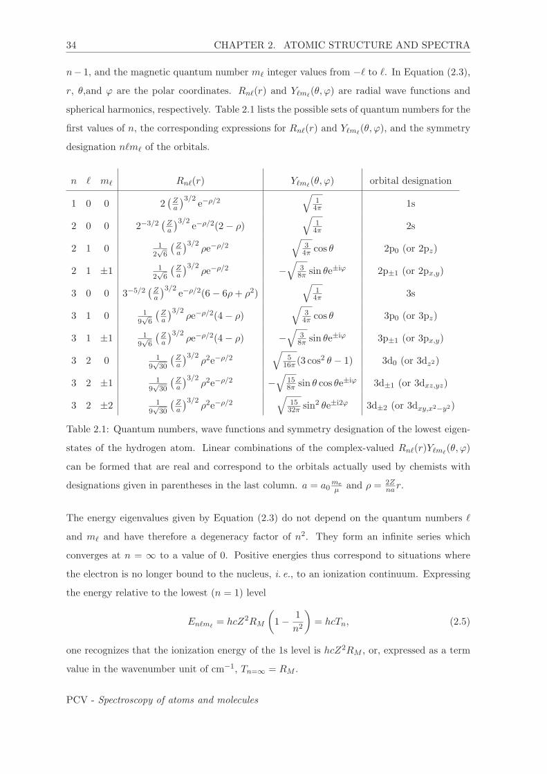
n− 1, and the magnetic quantum number m� integer values from −� to �. In Equation (2.3),
r, θ,and ϕ are the polar coordinates. Rn�(r) and Y�m�(θ, ϕ) are radial wave functions and
spherical harmonics, respectively. Table 2.1 lists the possible sets of quantum numbers for the
first values of n, the corresponding expressions for Rn�(r) and Y�m�(θ, ϕ), and the symmetry
designation n�m� of the orbitals.
n � m� Rn�(r) Y�m�(θ, ϕ) orbital designation
1 0 0 2(Za
)3/2e−ρ/2
√14π 1s
2 0 0 2−3/2(Za
)3/2e−ρ/2(2− ρ)
√14π 2s
2 1 0 12√6
(Za
)3/2ρe−ρ/2
√34π cos θ 2p0 (or 2pz)
2 1 ±1 12√6
(Za
)3/2ρe−ρ/2 −
√38π sin θe±iϕ 2p±1 (or 2px,y)
3 0 0 3−5/2(Za
)3/2e−ρ/2(6− 6ρ+ ρ2)
√14π 3s
3 1 0 19√6
(Za
)3/2ρe−ρ/2(4− ρ)
√34π cos θ 3p0 (or 3pz)
3 1 ±1 19√6
(Za
)3/2ρe−ρ/2(4− ρ) −
√38π sin θe±iϕ 3p±1 (or 3px,y)
3 2 0 19√30
(Za
)3/2ρ2e−ρ/2
√5
16π (3 cos2 θ − 1) 3d0 (or 3dz2)
3 2 ±1 19√30
(Za
)3/2ρ2e−ρ/2 −
√158π sin θ cos θe±iϕ 3d±1 (or 3dxz,yz)
3 2 ±2 19√30
(Za
)3/2ρ2e−ρ/2
√1532π sin2 θe±i2ϕ 3d±2 (or 3dxy,x2−y2)
Table 2.1: Quantum numbers, wave functions and symmetry designation of the lowest eigen-
states of the hydrogen atom. Linear combinations of the complex-valued Rn�(r)Y�m�(θ, ϕ)
can be formed that are real and correspond to the orbitals actually used by chemists with
designations given in parentheses in the last column. a = a0meμ and ρ = 2Z
na r.
The energy eigenvalues given by Equation (2.3) do not depend on the quantum numbers �
and m� and have therefore a degeneracy factor of n2. They form an infinite series which
converges at n = ∞ to a value of 0. Positive energies thus correspond to situations where
the electron is no longer bound to the nucleus, i. e., to an ionization continuum. Expressing
the energy relative to the lowest (n = 1) level
En�m�= hcZ2RM
(1− 1
n2
)= hcTn, (2.5)
one recognizes that the ionization energy of the 1s level is hcZ2RM , or, expressed as a term
value in the wavenumber unit of cm−1, Tn=∞ = RM .
PCV - Spectroscopy of atoms and molecules

2.1. ATOMIC STRUCTURE 35
The functions Ψn�m�(r, θ, φ) represent orbitals and describe the bound states of one-electron
atoms; the product Ψ∗n�m�Ψn�m�
= |Ψn�m�|2 represents the probability density of finding the
electron at the position (r, θ, ϕ) and implies the following general behavior:
• The average distance between the electron and the nucleus is proportional to n2, in
accordance with Bohr’s model of the hydrogen atom, which predicts that the classical
radius of the electron orbit should grow with n as a0n2, a0 being the Bohr radius
(a0 = 0.52917721092(17)× 10−10m).
• The probability of finding the electron in the immediate vicinity of the nucleus, i. e.,
within a sphere of radius on the order of a0, decreases with n−3. This implies that all
physical properties which depend on this probability, such as the excitation probability
from the ground state, or the radiative decay rate to the ground state should also scale
with n−3.
The orbital angular momentum quantum number �, which comes naturally in the solution of
the Schrodinger equation of the hydrogen atom, is also a symmetry label of the corresponding
quantum states. Indeed, the 2�+ 1 functions Ψn�m�(r, θ, ϕ) with m� = −�,−�+ 1, . . . , � are
designated by letters as s (� = 0), p (� = 1), d (� = 2), f (� = 3), g (� = 4), with subsequent
labels in alphabetical order, i. e., h, i, k, l, etc. for � = 5, 6, 7, 8, etc. The distinction between
electronic orbitals and electronic states is useful in polyelectronic atoms.
The operators �2 and �z describing the squared norm of the orbital angular momentum vector
and its projection along the z axis commute with H and with each other. The spherical
harmonics Y�m�(θ, ϕ) are thus also eigenfunctions of �2 and �z with eigenvalues given by the
eigenvalue equations
�2Y�m�(θ, ϕ) = �
2�(�+ 1)Y�m�(θ, ϕ) (2.6)
and
�zY�m�(θ, ϕ) = �m�Y�m�
(θ, ϕ). (2.7)
PCV - Spectroscopy of atoms and molecules
36 CHAPTER 2. ATOMIC STRUCTURE AND SPECTRA
2.1.2 Polyelectronic atoms
Reminder: Exact and approximate separability of the Schrodinger equation
We consider a system of two particles described by the Hamiltonian:
H = H1(p1, q1) + H2(p2, q2) (2.8)
Each operator Hi only depends on the momentum operator pi and coordinates qi of
particle i. In such a case, a solution of the Scrodinger equation
HΨn = EnΨn (2.9)
can be written as a product
Ψn = φn1,1φn2,2, (2.10)
and the eigenvalues as a sum
En = En1,1 + En2,2. (2.11)
Inserting Equation (2.10) and Equation (2.11) into Equation (2.9) one obtains:
(H1 + H2
)φn1,1φn2,2 = (En1,1 + En2,2)φn1,1φn2,2, (2.12)
i. e. H1φn1,1 = En1,1φn1,1 and H2φn2,2 = En2,2φn2,2.
In general the wavefunction of n non-interacting particles is the product of the one-
particle wavefunctions and the total energy is the sum of the one-particle energies.
In many cases the Schrodinger equation is nearly separable. This is the case when
H = H1(p1, q1) + H2(p2, q2) + H ′, (2.13)
where the expectation values of H ′ are much smaller than those of H1 and H2. The
functions φn1,1(q1)φn2,2(q2) are very similar to the exact eigenfunctions of H and serve
as a good approximation for them. In such a case, perturbation theory is a good approach
to improve the approximation.
The Hamiltonian for atoms with more than one electron can be written as follows:
H =
N∑i=1
(p2i2me
− Ze2
4πε0ri
)︸ ︷︷ ︸
hi
+
N∑i=1
N∑j>i
e2
4πε0rij︸ ︷︷ ︸H′
+H ′′ , (2.14)
where H ′′ represents all weak interactions not contained in hi and H ′, cannot be solved
analytically. If H ′ and H ′′ in Equation (2.14) are neglected, H becomes separable in N
PCV - Spectroscopy of atoms and molecules
2.1. ATOMIC STRUCTURE 37
one-electron operators hi(pi, qi) with hi(pi, qi)φj(qi) = εjφj(qi) (to simplify the notation, we
use in the following the notation qi instead of qi to designate all spatial xi, yi, zi and spin msi
coordinates of the polyelectron wave function)
H0 =
N∑i=1
hi(pi, qi), (2.15)
with eigenfunctions
Ψk(q1, . . . , qN ) = φk1(q1)φk2(q2) . . . φkN (qN ) (2.16)
and eigenvalues
Ek = εk1 + εk2 + ...+ εkN , (2.17)
where φj(qi) = Rnj�j (ri)Y�jm�j(θi, ϕi)σmsj
represents a spin orbital with σmsjbeing the spin
part of the orbital, either α for msj = 1/2 or β for msj = −1/2 .
The electron wave function in Equation (2.16) gives the occupation of the atomic orbitals
and represents a given electron configuration e. g., for the atom of lithium (Li), one gets:
Ψ1(q1, q2, q3) = 1sα(q1), 1sβ(q2), 2sα(q3). Neglecting the electron-repulsion term H ′ in Equa-
tion (2.14) is a very crude approximation, and it needs to be considered to get a realistic
estimation of the eigenfunctions and eigenvalues of H. A way to consider H ′ without affect-
ing the product form of Equation (2.16) is to introduce, for each electron, a potential energy
term describing the interaction with the mean field of all other electrons. Iteratively solv-
ing one-electron problems and modifying the mean-field potential term lead to the so-called
“Hartree-Fock Self-Consistent Field” (HF-SCF) wave functions, which still have the form
of Equation (2.16) for a single electronic configuration but now incorporate most effects of
the electron-electron repulsion except their instantaneous correlation. Because polyelectronic
atoms are also spherically symmetric the angular part of the improved orbitals can also be
described by spherical harmonics Y�m�(θi, ϕi). However, the radial functions Rn�(ri) and the
orbital energies (εj) differ from the hydrogenic case because of the electron-electron repulsion
term H ′.
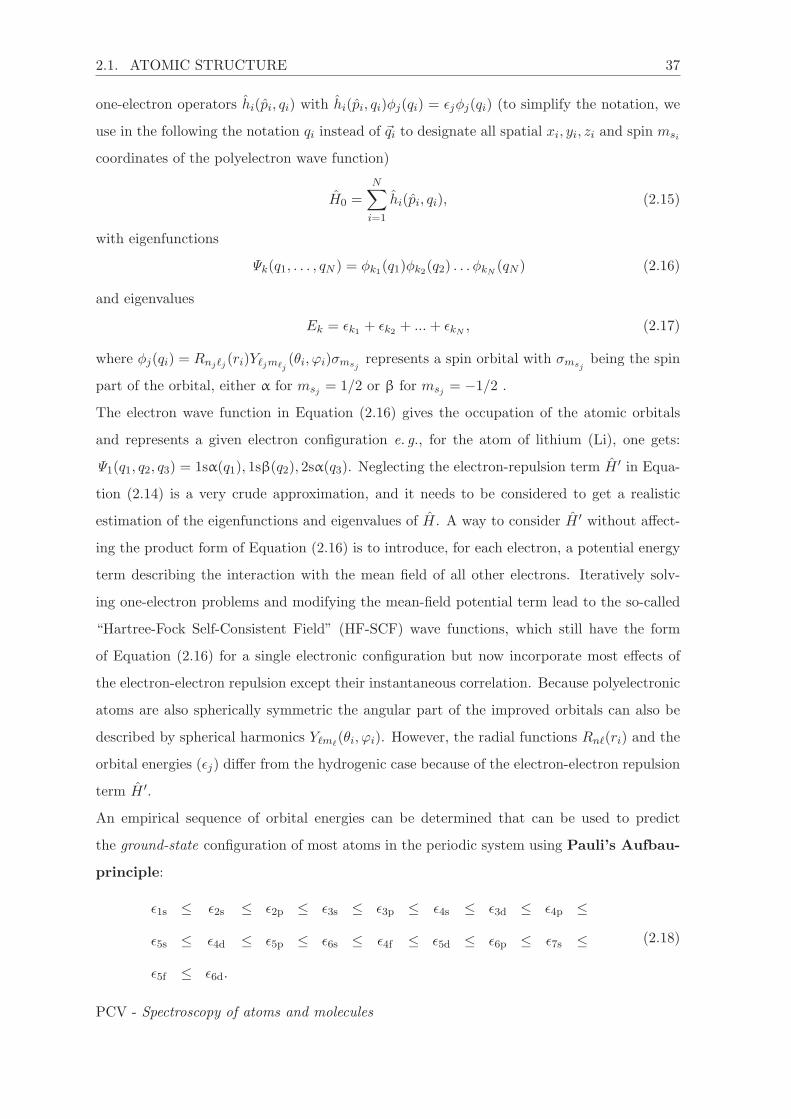
An empirical sequence of orbital energies can be determined that can be used to predict
the ground-state configuration of most atoms in the periodic system using Pauli’s Aufbau-
principle:
ε1s ≤ ε2s ≤ ε2p ≤ ε3s ≤ ε3p ≤ ε4s ≤ ε3d ≤ ε4p ≤
ε5s ≤ ε4d ≤ ε5p ≤ ε6s ≤ ε4f ≤ ε5d ≤ ε6p ≤ ε7s ≤
ε5f ≤ ε6d.
(2.18)
PCV - Spectroscopy of atoms and molecules

38 CHAPTER 2. ATOMIC STRUCTURE AND SPECTRA
This sequence of orbital energies can be qualitatively explained by considering the shielding
of the nuclear charge by electrons in inner shells and the decrease, with increasing value of �,
of the penetrating character of the orbitals.
For most purposes and in many atoms the product form of Equation (2.16) represents an
adequate approximation of the N -electron wave function. However, Equation (2.16) is, not
compatible with the generalized Pauli principle. Indeed, electrons have a half-integer spin
quantum number (s = 1/2) and polyelectronic wave functions must be antisymmetric with
respect to the exchange (permutation) of the coordinates of any pair of electrons. Equa-
tion (2.16) must therefore be antisymmetrized with respect to such an exchange of coordi-
nates. This is achieved by writing the wave functions as determinants of the type:
Ψ(q1, . . . , qN ) =1√N !
det
∣∣∣∣∣∣∣∣∣∣∣∣∣∣∣∣∣∣∣∣∣∣
φk1(q1) φk1(q2) . . . φk1(qN )
φk2(q1) φk2(q2) . . . φk2(qN )
.
.
.
φkN (q1) . . . . . . φkN (qN )
∣∣∣∣∣∣∣∣∣∣∣∣∣∣∣∣∣∣∣∣∣∣
(2.19)
in which all φi are different spin orbitals. Such determinants are called Slater determi-
nants and represent suitable N -electron wave functions which automatically fulfill the Pauli
principle for fermions. Indeed, exchanging two columns in a determinant, i. e., permuting
the coordinates of two electrons, automatically changes the sign of the determinant. The
determinant of a matrix with two identical rows is zero so that Equation (2.19) is also in
accord with Pauli’s exclusion principle, namely that any configuration with two electrons in
the same spin orbital is forbidden. This is not surprising given that Pauli’s exclusion prin-
ciple can be regarded as a consequence of the generalized Pauli principle for fermions. The
ground-state configuration of an atom can thus be obtained by filling the orbitals in order
of increasing energy (see Equation (2.18)) with two electrons, one with ms = 1/2, the other
with ms = −1/2, a procedure known as the Pauli’s Aufbau-principle.
2.1.3 Singlet and triplet states
The generalized Pauli principle for fermions also restricts the number of possible wave func-
tions associated with a given configuration, as illustrated with the ground electronic config-
uration of the carbon atom in the following example.
PCV - Spectroscopy of atoms and molecules
2.1. ATOMIC STRUCTURE 39
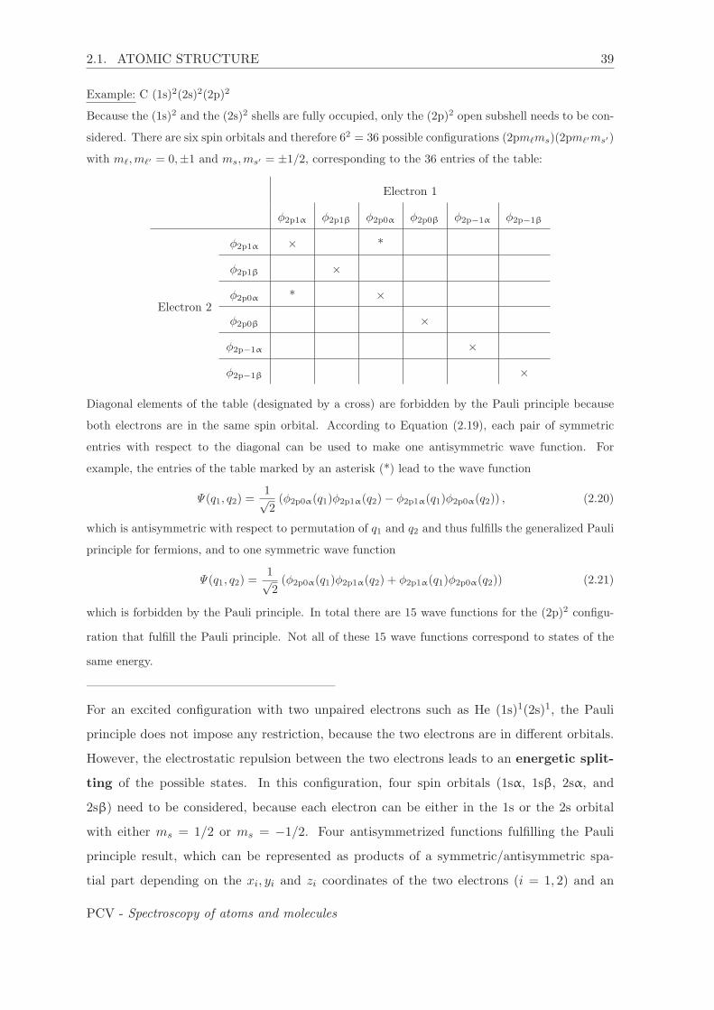
Example: C (1s)2(2s)2(2p)2
Because the (1s)2 and the (2s)2 shells are fully occupied, only the (2p)2 open subshell needs to be con-
sidered. There are six spin orbitals and therefore 62 = 36 possible configurations (2pm�ms)(2pm�′ms′)
with m�,m�′ = 0,±1 and ms,ms′ = ±1/2, corresponding to the 36 entries of the table:
Electron 1
φ2p1α φ2p1β φ2p0α φ2p0β φ2p−1α φ2p−1β
Electron 2
φ2p1α × *
φ2p1β ×φ2p0α * ×φ2p0β ×φ2p−1α ×φ2p−1β ×
Diagonal elements of the table (designated by a cross) are forbidden by the Pauli principle because
both electrons are in the same spin orbital. According to Equation (2.19), each pair of symmetric
entries with respect to the diagonal can be used to make one antisymmetric wave function. For
example, the entries of the table marked by an asterisk (*) lead to the wave function
Ψ(q1, q2) =1√2(φ2p0α(q1)φ2p1α(q2)− φ2p1α(q1)φ2p0α(q2)) , (2.20)
which is antisymmetric with respect to permutation of q1 and q2 and thus fulfills the generalized Pauli
principle for fermions, and to one symmetric wave function
Ψ(q1, q2) =1√2(φ2p0α(q1)φ2p1α(q2) + φ2p1α(q1)φ2p0α(q2)) (2.21)
which is forbidden by the Pauli principle. In total there are 15 wave functions for the (2p)2 configu-
ration that fulfill the Pauli principle. Not all of these 15 wave functions correspond to states of the
same energy.
———————————————————
For an excited configuration with two unpaired electrons such as He (1s)1(2s)1, the Pauli
principle does not impose any restriction, because the two electrons are in different orbitals.
However, the electrostatic repulsion between the two electrons leads to an energetic split-
ting of the possible states. In this configuration, four spin orbitals (1sα, 1sβ, 2sα, and
2sβ) need to be considered, because each electron can be either in the 1s or the 2s orbital
with either ms = 1/2 or ms = −1/2. Four antisymmetrized functions fulfilling the Pauli
principle result, which can be represented as products of a symmetric/antisymmetric spa-
tial part depending on the xi, yi and zi coordinates of the two electrons (i = 1, 2) and an
PCV - Spectroscopy of atoms and molecules
40 CHAPTER 2. ATOMIC STRUCTURE AND SPECTRA
antisymmetric/symmetric spin part (T= triplet, S=singlet):
1√2(1s(1)2s(2)− 1s(2)2s(1))α(1)α(2) = ΨT,MS=1 (2.22)
1√2(1s(1)2s(2)− 1s(2)2s(1))β(1)β(2) = ΨT,MS=−1 (2.23)
1√2(1s(1)2s(2)− 1s(2)2s(1))
1√2[α(1)β(2) + α(2)β(1)] = ΨT,MS=0 (2.24)
1√2(1s(1)2s(2) + 1s(2)2s(1))
1√2(α(1)β(2)− α(2)β(1)) = ΨS,MS=0, (2.25)
where the notation 1s(i)α(i) has been used to designate electron i being in the 1s orbital with
spin projection quantum number ms = 1/2.
The first three functions (Equations (2.22), (2.23) and (2.24)), with MS = ms1+ms2 = ±1, 0,
have an antisymmetric spatial part and a symmetric electron-spin part with respect to the
permutation of the two electrons. These three functions represent the three components of
a triplet (S = 1) state. The fourth function has a symmetric spatial and an antisymmetric
electron-spin part with MS = 0 and represents a singlet (S = 0) state. These results are
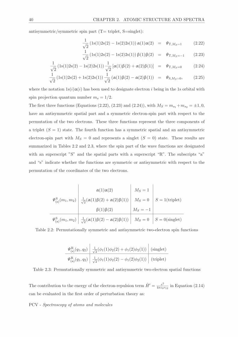
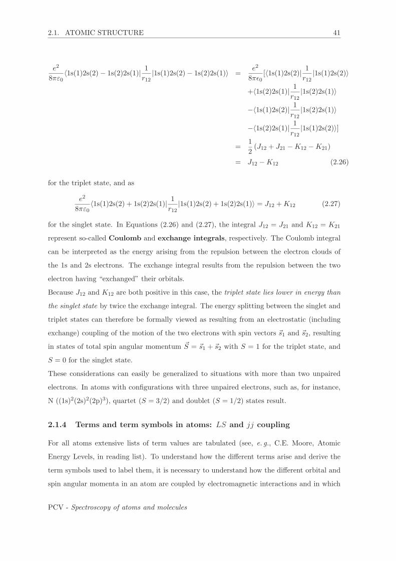
summarized in Tables 2.2 and 2.3, where the spin part of the wave functions are designated
with an superscript ”S” and the spatial parts with a superscript “R”. The subscripts “a”
and “s” indicate whether the functions are symmetric or antisymmetric with respect to the
permutation of the coordinates of the two electrons.
α(1)α(2) MS = 1
ΨS(s)(m1,m2)
1√2(α(1)β(2) + α(2)β(1)) MS = 0 S = 1(triplet)
β(1)β(2) MS = −1
ΨS(a)(m1,m2)
1√2(α(1)β(2)− α(2)β(1)) MS = 0 S = 0(singlet)
Table 2.2: Permutationally symmetric and antisymmetric two-electron spin functions
ΨR(s)(q1, q2)
1√2(φ1(1)φ2(2) + φ1(2)φ2(1)) (singlet)
ΨR(a)(q1, q2)
1√2(φ1(1)φ2(2)− φ1(2)φ2(1)) (triplet)
Table 2.3: Permutationally symmetric and antisymmetric two-electron spatial functions
The contribution to the energy of the electron-repulsion term H ′ = e2
4πε0r12in Equation (2.14)
can be evaluated in the first order of perturbation theory as:
PCV - Spectroscopy of atoms and molecules
2.1. ATOMIC STRUCTURE 41
e2
8πε0〈1s(1)2s(2)− 1s(2)2s(1)| 1
r12|1s(1)2s(2)− 1s(2)2s(1)〉 =
e2
8πε0[〈1s(1)2s(2)| 1
r12|1s(1)2s(2)〉
+〈1s(2)2s(1)| 1
r12|1s(2)2s(1)〉
−〈1s(1)2s(2)| 1
r12|1s(2)2s(1)〉
−〈1s(2)2s(1)| 1
r12|1s(1)2s(2)〉]
=1
2(J12 + J21 −K12 −K21)
= J12 −K12 (2.26)
for the triplet state, and as
e2
8πε0〈1s(1)2s(2) + 1s(2)2s(1)| 1
r12|1s(1)2s(2) + 1s(2)2s(1)〉 = J12 +K12 (2.27)
for the singlet state. In Equations (2.26) and (2.27), the integral J12 = J21 and K12 = K21
represent so-called Coulomb and exchange integrals, respectively. The Coulomb integral
can be interpreted as the energy arising from the repulsion between the electron clouds of
the 1s and 2s electrons. The exchange integral results from the repulsion between the two
electron having “exchanged” their orbitals.
Because J12 and K12 are both positive in this case, the triplet state lies lower in energy than
the singlet state by twice the exchange integral. The energy splitting between the singlet and
triplet states can therefore be formally viewed as resulting from an electrostatic (including
exchange) coupling of the motion of the two electrons with spin vectors s1 and s2, resulting
in states of total spin angular momentum S = s1 + s2 with S = 1 for the triplet state, and
S = 0 for the singlet state.
These considerations can easily be generalized to situations with more than two unpaired
electrons. In atoms with configurations with three unpaired electrons, such as, for instance,
N ((1s)2(2s)2(2p)3), quartet (S = 3/2) and doublet (S = 1/2) states result.
2.1.4 Terms and term symbols in atoms: LS and jj coupling
For all atoms extensive lists of term values are tabulated (see, e. g., C.E. Moore, Atomic
Energy Levels, in reading list). To understand how the different terms arise and derive the
term symbols used to label them, it is necessary to understand how the different orbital and
spin angular momenta in an atom are coupled by electromagnetic interactions and in which
PCV - Spectroscopy of atoms and molecules
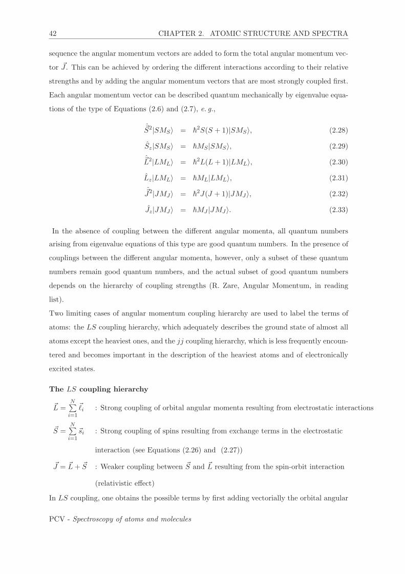
42 CHAPTER 2. ATOMIC STRUCTURE AND SPECTRA
sequence the angular momentum vectors are added to form the total angular momentum vec-
tor J . This can be achieved by ordering the different interactions according to their relative
strengths and by adding the angular momentum vectors that are most strongly coupled first.
Each angular momentum vector can be described quantum mechanically by eigenvalue equa-
tions of the type of Equations (2.6) and (2.7), e. g.,
S2|SMS〉 = �2S(S + 1)|SMS〉, (2.28)
Sz|SMS〉 = �MS |SMS〉, (2.29)
L2|LML〉 = �2L(L+ 1)|LML〉, (2.30)
Lz|LML〉 = �ML|LML〉, (2.31)
J2|JMJ〉 = �2J(J + 1)|JMJ〉, (2.32)
Jz|JMJ〉 = �MJ |JMJ〉. (2.33)
In the absence of coupling between the different angular momenta, all quantum numbers
arising from eigenvalue equations of this type are good quantum numbers. In the presence of
couplings between the different angular momenta, however, only a subset of these quantum
numbers remain good quantum numbers, and the actual subset of good quantum numbers
depends on the hierarchy of coupling strengths (R. Zare, Angular Momentum, in reading
list).
Two limiting cases of angular momentum coupling hierarchy are used to label the terms of
atoms: the LS coupling hierarchy, which adequately describes the ground state of almost all
atoms except the heaviest ones, and the jj coupling hierarchy, which is less frequently encoun-
tered and becomes important in the description of the heaviest atoms and of electronically
excited states.
The LS coupling hierarchy
L =N∑i=1
�i : Strong coupling of orbital angular momenta resulting from electrostatic interactions
S =N∑i=1
si : Strong coupling of spins resulting from exchange terms in the electrostatic
interaction (see Equations (2.26) and (2.27))
J = L+ S : Weaker coupling between S and L resulting from the spin-orbit interaction
(relativistic effect)
In LS coupling, one obtains the possible terms by first adding vectorially the orbital angular
PCV - Spectroscopy of atoms and molecules

2.1. ATOMIC STRUCTURE 43
momenta �i of the electrons to form a resultant total orbital angular momentum L. Then,
the total electron spin S is determined by vectorial addition of the spins si of all electrons.
Finally, the total angular momentum J is determined by adding vectorially S and L. For a
two-electron system, one obtains:
L = �1 + �2; L = |�1 − �2|, |�1 − �2|+ 1, . . . , �1 + �2 (2.34)
ML = m�1 +m�2 = −L,−L+ 1, . . . , L (2.35)
S = s1 + s2; S = 1, 0 (2.36)
MS = ms1 +ms2 = −S,−S + 1, . . . , S (2.37)
J = L+ S; J = |L− S|, |L− S|+ 1, . . . , L+ S (2.38)
MJ = MS +ML = −J,−J + 1, . . . , J. (2.39)
The angular momentum quantum numbers L, S and J that arise in Equations (2.34), (2.36),
and (2.38) from the addition of the pairs of coupled vectors (�1, �2), (s1, s2) and (L, S),
respectively, can be derived from angular momentum algebra as explained in most quantum
mechanics textbooks.
The different terms (L, S, J) that are obtained for the possible values of L, S and J in
Equations (2.34), (2.36), and (2.38) are written in compact form as term symbols
2S+1LJ . (2.40)
However, not all terms that are predicted by Equations (2.34), (2.36), and (2.38) are al-
lowed by the Pauli principle. This is best explained by deriving the possible terms of the C
(1s)2(2s)2(2p)2 configuration in the following example.
———————————————————
Example: C (1s)2(2s)2(2p)2. Only the partially filled 2p subshell needs to be considered. In this case
l1 = 1, l2 = 1 and s1 = s2 = 1/2. From Equations (2.34), (2.36), and (2.38) one obtains, neglecting
the Pauli principle:
L = 0(S), 1(P), 2(D)
S = 0(singlet), 1(triplet)
J = 0, 1, 2, 3
which leads to the following terms:
Term 1S03S1
1P13P0
3P13P2
1D23D1
3D23D3
Degeneracy factor gJ = 2J + 1 1 3 3 1 3 5 5 3 5 7
PCV - Spectroscopy of atoms and molecules
44 CHAPTER 2. ATOMIC STRUCTURE AND SPECTRA
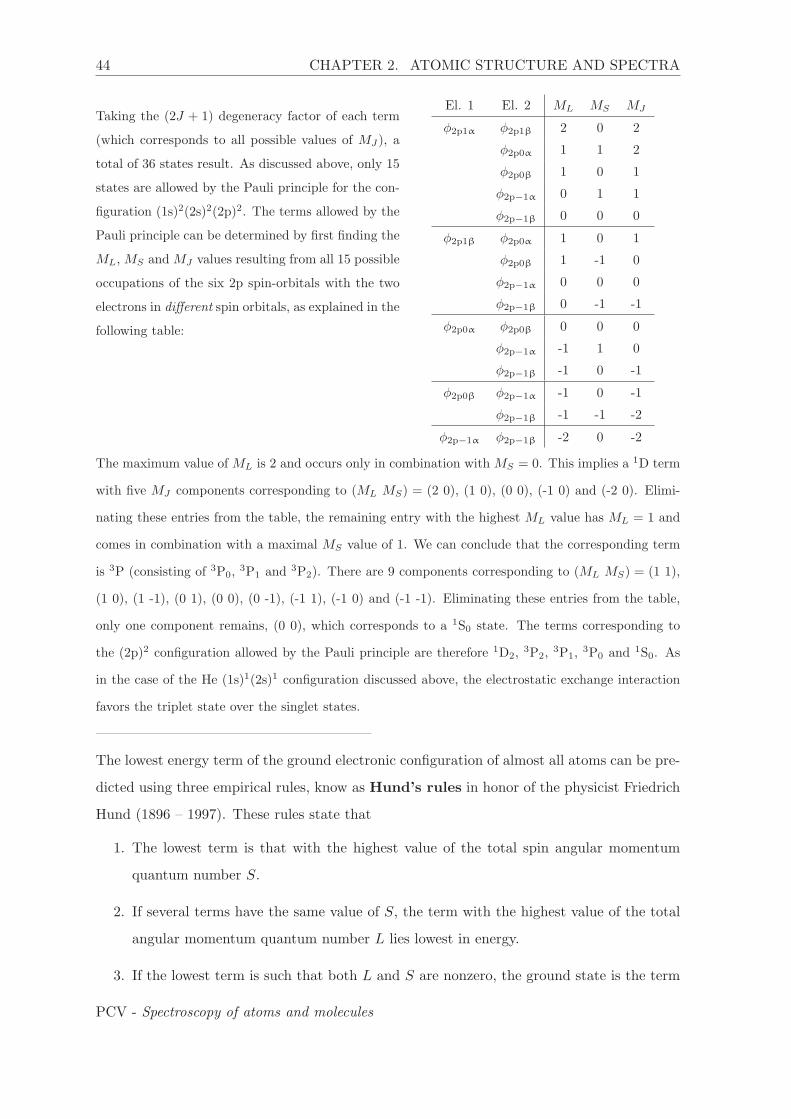
Taking the (2J + 1) degeneracy factor of each term
(which corresponds to all possible values of MJ), a
total of 36 states result. As discussed above, only 15
states are allowed by the Pauli principle for the con-
figuration (1s)2(2s)2(2p)2. The terms allowed by the
Pauli principle can be determined by first finding the
ML, MS and MJ values resulting from all 15 possible
occupations of the six 2p spin-orbitals with the two
electrons in different spin orbitals, as explained in the
following table:
El. 1 El. 2 ML MS MJ
φ2p1α φ2p1β 2 0 2
φ2p0α 1 1 2
φ2p0β 1 0 1
φ2p−1α 0 1 1
φ2p−1β 0 0 0
φ2p1β φ2p0α 1 0 1
φ2p0β 1 -1 0
φ2p−1α 0 0 0
φ2p−1β 0 -1 -1
φ2p0α φ2p0β 0 0 0
φ2p−1α -1 1 0
φ2p−1β -1 0 -1
φ2p0β φ2p−1α -1 0 -1
φ2p−1β -1 -1 -2
φ2p−1α φ2p−1β -2 0 -2
The maximum value of ML is 2 and occurs only in combination with MS = 0. This implies a 1D term
with five MJ components corresponding to (ML MS) = (2 0), (1 0), (0 0), (-1 0) and (-2 0). Elimi-
nating these entries from the table, the remaining entry with the highest ML value has ML = 1 and
comes in combination with a maximal MS value of 1. We can conclude that the corresponding term
is 3P (consisting of 3P0,3P1 and 3P2). There are 9 components corresponding to (ML MS) = (1 1),
(1 0), (1 -1), (0 1), (0 0), (0 -1), (-1 1), (-1 0) and (-1 -1). Eliminating these entries from the table,
only one component remains, (0 0), which corresponds to a 1S0 state. The terms corresponding to
the (2p)2 configuration allowed by the Pauli principle are therefore 1D2,3P2,
3P1,3P0 and 1S0. As
in the case of the He (1s)1(2s)1 configuration discussed above, the electrostatic exchange interaction
favors the triplet state over the singlet states.
———————————————————
The lowest energy term of the ground electronic configuration of almost all atoms can be pre-
dicted using three empirical rules, know as Hund’s rules in honor of the physicist Friedrich
Hund (1896 – 1997). These rules state that
1. The lowest term is that with the highest value of the total spin angular momentum
quantum number S.
2. If several terms have the same value of S, the term with the highest value of the total
angular momentum quantum number L lies lowest in energy.
3. If the lowest term is such that both L and S are nonzero, the ground state is the term
PCV - Spectroscopy of atoms and molecules

2.1. ATOMIC STRUCTURE 45
component with J = |L−S| if the partially filled subshell is less than half full, and the
term component with J = L+ S if the partially filled subshell is more than half full.
According to Hund’s rules, the ground state of C is the term component 3P0, and the ground
state of F is the term component 2P3/2, in agreement with experimental results. Hund’s rules
do not reliably predict the energetic ordering of electronically excited states.
The energy level splittings of the components of a term 2S+1L can be described by considering
the effect of the effective spin-orbit operator
HSO =hcA
�2L · S (2.41)
on the basis functions |LSJ〉 with J = L + S. In Equation (2.41), the spin-orbit coupling
constant A is expressed in cm−1. From J2 = L2 + S2 + 2L · S one finds
L · S =1
2
[J2 − L2 − S2
]. (2.42)
The diagonal matrix elements of HSO, which represent the first-order corrections to the
energies in a perturbation theory treatment, are
〈LSJ |HSO|LSJ〉 = 1
2hcA[J(J + 1)− L(L+ 1)− S(S + 1)], (2.43)
from which one sees that two components of a term with J and J +1 are separated in energy
by hcA(J + 1). Hund’s third rule implies that the spin-orbit coupling constant A is positive
in ground terms arising from less than half-full subshells and negative in ground terms arising
from more than half-full subshells.
To illustrate the main conclusions of this subsection, Figure 2.1 shows schematically by which
interactions the 15 states of the ground-state configuration of C can be split. The strong
electrostatic interactions (including exchange) lead to a splitting into three terms 3P, 1D and
1S. The weaker spin-orbit interaction splits the ground 3P term into three components 3P0,
3P1 and3P2. Each term component can be further split into (2J+1) MJ levels by an external
magnetic field, an effect known as the Zeeman effect.
PCV - Spectroscopy of atoms and molecules
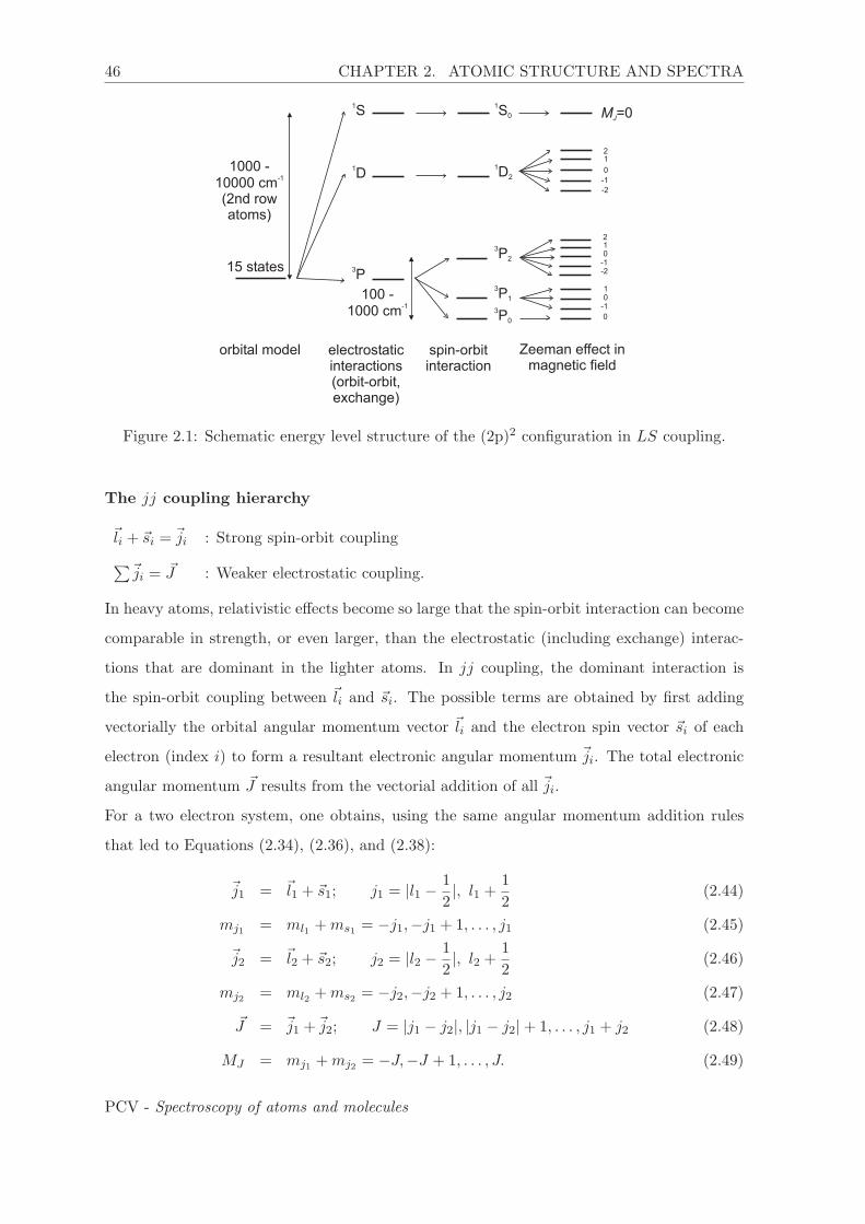
46 CHAPTER 2. ATOMIC STRUCTURE AND SPECTRA
Figure 2.1: Schematic energy level structure of the (2p)2 configuration in LS coupling.
The jj coupling hierarchy
li + si = ji : Strong spin-orbit coupling
∑ji = J : Weaker electrostatic coupling.
In heavy atoms, relativistic effects become so large that the spin-orbit interaction can become
comparable in strength, or even larger, than the electrostatic (including exchange) interac-
tions that are dominant in the lighter atoms. In jj coupling, the dominant interaction is
the spin-orbit coupling between li and si. The possible terms are obtained by first adding
vectorially the orbital angular momentum vector li and the electron spin vector si of each
electron (index i) to form a resultant electronic angular momentum ji. The total electronic
angular momentum J results from the vectorial addition of all ji.
For a two electron system, one obtains, using the same angular momentum addition rules
that led to Equations (2.34), (2.36), and (2.38):
j1 = l1 + s1; j1 = |l1 − 1
2|, l1 +
1
2(2.44)
mj1 = ml1 +ms1 = −j1,−j1 + 1, . . . , j1 (2.45)
j2 = l2 + s2; j2 = |l2 − 1
2|, l2 +
1
2(2.46)
mj2 = ml2 +ms2 = −j2,−j2 + 1, . . . , j2 (2.47)
J = j1 +j2; J = |j1 − j2|, |j1 − j2|+ 1, . . . , j1 + j2 (2.48)
MJ = mj1 +mj2 = −J,−J + 1, . . . , J. (2.49)
PCV - Spectroscopy of atoms and molecules

2.1. ATOMIC STRUCTURE 47
The total orbital and spin angular momentum quantum numbers L and S are no longer
defined in jj coupling. Instead, the terms are now specified by a different set of angular
momentum quantum numbers: the total angular momentum ji of all electrons (index i) in
partially filled subshells and the total angular momentum quantum number J of the atom.
A convenient way to label the terms is (j1, j2, . . . , jN )J .
———————————————————
Example: The (np)1((n+ 1)s)1 excited configuration:
LS coupling: S = 0, 1; L = 1. Termsymbols: 1P1,3P0,1,2, which give rise to 12 states.
jj coupling: l1 = 1, s1 = 12 , j1 = 1
2 ,32 and l2 = 0, s2 = 1
2 , j2 = 12 . Termsymbols: [(j1, j2)J ] :
( 12 ,12 )0; (
12 ,
12 )1; (
32 ,
12 )1; (
32 ,
12 )2, which also gives rise to 12 states.
———————————————————
The evolution from LS coupling to jj coupling can be observed by looking at the evolution of
the energy level structure associated with a given configuration as one moves down a column
in the periodic table. Figure 2.2 illustrates schematically how the energy levels arising from
the (np)1((n + 1)s)1 excited configuration are grouped according to LS coupling for n = 2
and 3 (C and Si) and according to jj coupling for n = 6 (Pb). The main splitting between
the (1/2, 1/2)0,1 and the (3/2, 1/2)1,2 states of Pb is actually much larger than the splitting
between the 3P and 1P terms. Figure 2.2 is a so-called correlation diagram, which represents
how the energy level structure of a given system (here the states of the (np)1((n+1)s)1 con-
figuration) evolves as a function of one or more system parameters (here the magnitude of the
spin-orbit and electrostatic interactions). States with the same values of all good quantum
numbers (here J) are usually connected by lines and do not cross in a correlation diagram.
1P
J=0
1st + 2nd rowC, Si
1
2
3P
J=1
(1/2, 1/2)J=1
J=0
(3/2, 1/2)J=1
J=2
Pb
Figure 2.2: Correlation diagram depicting schematically, and not to scale, how the term
values for the (np)((n + 1)s) configuration evolve from C, for which the LS coupling limit
represents a good description, to Pb, the level structure of which is more adequately described
by the jj coupling limit.
PCV - Spectroscopy of atoms and molecules

48 CHAPTER 2. ATOMIC STRUCTURE AND SPECTRA
The actual evolution of the energy level structure in the series C, Si, Ge, Sn and Pb, drawn
to scale in Figure 2.3 using reference data on atomic term values, enables one to see quan-
titatively the effects of the gradual increase of the spin-orbit coupling. For the comparison,
the zero point of the energy scale was placed at the center of gravity of the energy level
structure. In C, the spin-orbit interaction is weaker than the electrostatic interactions, and
the spin-orbit splittings of the 3P state are hardly recognizable on the scale of the figure. In
Pb, it is stronger than the electrostatic interactions and determines the main splitting of the
energy level structure.
C
0
1
J
3P
1P
12
012
11
2
1
0
1
0
1
2
1
2
1
0
(3/2,1/2)
(1/2,1/2)
PbSi Ge Sn
0
E hc/ ( cm )-1
5000
- 10000
- 5000
Figure 2.3: Evolution from LS coupling to jj coupling with the example of the term values of
the (np)1((n+1)s)1 configuration of C, Si, Ge, Sn and Pb. The terms symbols are indicated
without the value of J on the left-hand side for the LS coupling limit and on the right-hand
side for the jj coupling limit. The values of J are indicated next to the horizontal bars
corresponding to the positions of the energy levels.
2.1.5 Hyperfine coupling
Magnetic moments arise in systems of charged particles with nonzero angular momenta to
which they are proportional. In the case of the orbital angular momentum of an electron, the
PCV - Spectroscopy of atoms and molecules
2.1. ATOMIC STRUCTURE 49
origin of the magnetic moment can be understood by considering the similarity between the
orbital motion of an electron in an atom and a ”classical” current generated by an electron
moving with velocity v in a circular loop or radius r. The magnetic moment is equal to
μ = − e
2mer ×mev = − e
2me
� = γ�. (2.50)
For the orbital motion of an electron in an atom, Equation (2.50) can be written using the
correspondence principle as
μ = γ� = −μB
�
�, (2.51)
where γ = −e/(2me) represents the magnetogyric ratio of the orbital motion and μB =
e�/(2me) = 9.27400968(20) × 10−24 JT−1 is the Bohr magneton. By analogy, similar equa-
tions can be derived for all other momenta. The electron spin s and the nuclear spin I, for
instance, give rise to the magnetic moments
μs = −geγs = geμB
�s, (2.52)
and
μI = γI I = gIμN
�
I, (2.53)
respectively, where ge is the so-called g value of the electron (ge = −2.0023193043622(15)),
γI is themagnetogyric ratio of the nucleus, μN = e�/(2mp) = 5.05078353(11)×10−27 JT−1
is the nuclear magneton (mp = 1.672621777(74)×10−27 kg is the mass of the proton), and gI
is the nuclear g factor (gp = 5.585 for the proton). Because μN/μB = me/mp, the magnetic
moments resulting from the electronic orbital and spin motions are typically 2 to 3 orders of
magnitude larger than the magnetic dipole moments (and higher moments) of nuclear spins.
The spin-orbit interaction is in general much stronger than the interactions involving nuclear
spins. The hyperfine interaction can therefore be described as an interaction between I, with
magnetic moment (gIμN/�)I, and J , with magnetic moment
μJ = gJγ J, (2.54)
rather than as two separate interactions of I with L and S. In Equation (2.54), gJ is the g
factor of the LS-coupled state, also called Lande g factor, and is given in good approximation
by
gJ = 1 +J(J + 1) + S(S + 1)− L(L+ 1)
2J(J + 1). (2.55)
PCV - Spectroscopy of atoms and molecules

50 CHAPTER 2. ATOMIC STRUCTURE AND SPECTRA
The hyperfine interaction results in a total angular momentum vector F of norm |F | =
�√
F (F + 1) and z-axis projection �MF . The possible values of the quantum numbers F
and MF can be determined using the usual angular momentum addition rules:
F = |J − I|, |J − I|+ 1, . . . , J + I, (2.56)
and
MF = −F, −F + 1, . . . , F. (2.57)
The hyperfine contribution to H arising from the interaction of μJ and μI is one of the terms
included in H ′′ in Equation (2.14) and is proportional to μI · μJ , and thus to I · J . Followingthe same argument as that used to derive Equation (2.43), one obtains
I · J =1
2
[F 2 − I2 − J2
](2.58)
with F = I + J and F 2 = I2 + J2 + 2I · J . The hyperfine energy shift of state |IJF 〉 is
therefore
〈IJF |ha�2
I · J |IJF 〉 = ha
2[F (F + 1)− I(I + 1)− J(J + 1)] (2.59)
as can be derived from Equation (2.58) and the eigenvalues of F 2, I2 and J2. In Equa-
tion (2.59), a is the hyperfine coupling constant in Hz. Note that choosing to express A in
cm−1 and a in Hz is the reason for the additional factor of c in Equation (2.41). Examples
of the fine and hyperfine structure of atoms will be given in Section 2.2.
2.2 Atomic spectra
2.2.1 Transition moments and selection rules
The intensity I(νfi) of a transition between an initial state of an atom or a molecule with
wave function Ψi and energy Ei and a final state with wave function Ψf and energy Ef is
proportional to the square of the matrix element Vfi, where the matrix V represents the
operator describing the interaction between the radiation field and the atom or the molecule
I(νfi) ∝ |〈Ψf |V |Ψi〉|2 = 〈f|V |i〉2 = V 2if . (2.60)
The transition is observed at the frequency νfi = |Ef − Ei|/h.A selection rule enables one to predict whether a transition can be observed or not on the
basis of symmetry arguments. If 〈Ψf |V |Ψi〉 = 0, the transition f ← i is said to be “forbidden”,
PCV - Spectroscopy of atoms and molecules
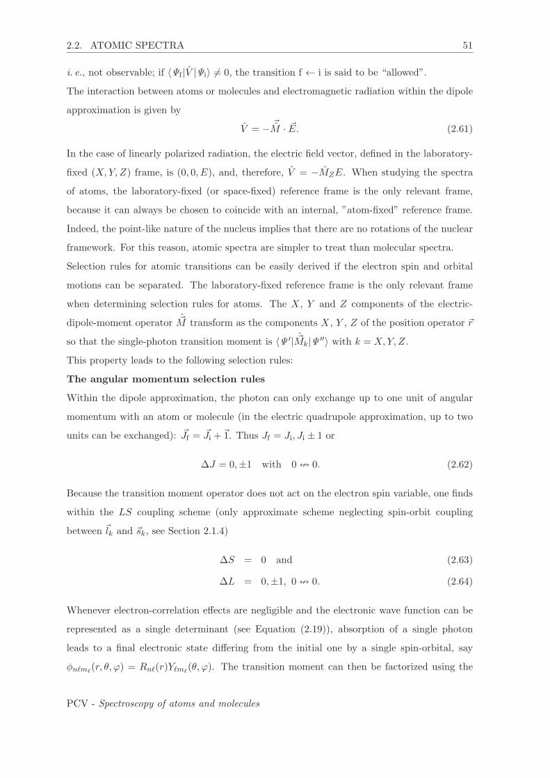
2.2. ATOMIC SPECTRA 51
i. e., not observable; if 〈Ψf |V |Ψi〉 = 0, the transition f ← i is said to be “allowed”.
The interaction between atoms or molecules and electromagnetic radiation within the dipole
approximation is given by
V = − M · E. (2.61)
In the case of linearly polarized radiation, the electric field vector, defined in the laboratory-
fixed (X,Y, Z) frame, is (0, 0, E), and, therefore, V = −MZE. When studying the spectra
of atoms, the laboratory-fixed (or space-fixed) reference frame is the only relevant frame,
because it can always be chosen to coincide with an internal, ”atom-fixed” reference frame.
Indeed, the point-like nature of the nucleus implies that there are no rotations of the nuclear
framework. For this reason, atomic spectra are simpler to treat than molecular spectra.
Selection rules for atomic transitions can be easily derived if the electron spin and orbital
motions can be separated. The laboratory-fixed reference frame is the only relevant frame
when determining selection rules for atoms. The X, Y and Z components of the electric-
dipole-moment operator M transform as the components X, Y , Z of the position operator r
so that the single-photon transition moment is 〈Ψ ′| Mk|Ψ ′′〉 with k = X,Y, Z.
This property leads to the following selection rules:
The angular momentum selection rules
Within the dipole approximation, the photon can only exchange up to one unit of angular
momentum with an atom or molecule (in the electric quadrupole approximation, up to two
units can be exchanged): Jf = Ji +1. Thus Jf = Ji, Ji ± 1 or
ΔJ = 0,±1 with 0 � 0. (2.62)
Because the transition moment operator does not act on the electron spin variable, one finds
within the LS coupling scheme (only approximate scheme neglecting spin-orbit coupling
between lk and sk, see Section 2.1.4)
ΔS = 0 and (2.63)
ΔL = 0,±1, 0 � 0. (2.64)
Whenever electron-correlation effects are negligible and the electronic wave function can be
represented as a single determinant (see Equation (2.19)), absorption of a single photon
leads to a final electronic state differing from the initial one by a single spin-orbital, say
φn�m�(r, θ, ϕ) = Rn�(r)Y�m�
(θ, ϕ). The transition moment can then be factorized using the
PCV - Spectroscopy of atoms and molecules

52 CHAPTER 2. ATOMIC STRUCTURE AND SPECTRA
relation z = r cos(θ) for radiation linearly polarized along z:
I(νfi) ∝∣∣∣〈φn′�′m′
�| M |φn′′�′′m′′
�〉∣∣∣2 = ∣∣∣〈Rn′�′ |r|Rn′′�′′〉〈Y�′m′
�| cos θ|Y�′′m′′
�〉∣∣∣2 (2.65)
The radial part of the integral is evaluated numerically whereas the angular part has analytical
solutions since Y�m�are spherical harmonics (see exercise 2). The angular part is responsible
for the selection rules
Δ� = �′ − �′′ = ±1 (2.66)
and
Δm = m′ −m′′ = 0 (2.67)
in the case of linearly polarized light.
The parity (Laporte) selection rule
The parity operator E∗ inverts the coordinates of all particles:
E∗Ψ(x1, . . . , zN ) = Ψ(−x1, . . . ,−zN ). (2.68)
Because the kinetic and potential energy operators in the Hamiltonian only depend on the
coordinates squared, the Hamiltonian commutes with the parity operator:
[E∗, H
]= 0 (2.69)
and therefore the eigenstates of the Hamiltonian are also eigenstates of the parity operator:
E∗Ψ(x1, . . . , zN ) = ±Ψ(x1, . . . , zN ). (2.70)
States with eigenvalue +1 have positive parity, states with eigenvalue −1 have negative
parity. The transition moment has negative parity:
E∗μ(x, y, z) = μ(−x,−y,−z) = −μ(x, y, z). (2.71)
Because the integral over a function of negative parity vanishes, dipole transitions are only
allowed between states of opposite parity:
+ ↔ −,+ � +,− � −. (2.72)
The same argumentation can easily be extended to the derivation of magnetic-dipole or
electric-quadrupole selection rules as well as selection rules for multiphoton processes.
PCV - Spectroscopy of atoms and molecules
2.2. ATOMIC SPECTRA 53
2.2.2 Spectra of hydrogen and other one-electron atoms
The spectra of hydrogen and hydrogen-like atoms have been of importance for the devel-
opment of quantum mechanics and for detecting and recognizing the significance of fine,
hyperfine and quantum-electrodynamics effects. They are also the source of precious infor-
mation on fundamental constants such as Rydberg’s constant and the fine-structure constant.
If fine, hyperfine, and quantum-electrodynamics effects are neglected, the energy level struc-
ture of the hydrogen atom is given by Equation (2.2) and is characterized by a high-degree
of degeneracy. The allowed electronic transitions can be predicted using Equation (2.66) and
their wavenumbers determined using Equation (2.73)
ν =RM
n′′2− RM
n′2(2.73)
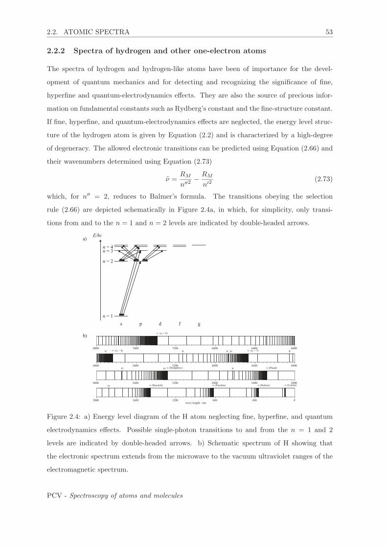
which, for n′′ = 2, reduces to Balmer’s formula. The transitions obeying the selection
rule (2.66) are depicted schematically in Figure 2.4a, in which, for simplicity, only transi-
tions from and to the n = 1 and n = 2 levels are indicated by double-headed arrows.
a)
s
E/hc
n = 1
n = 2
n = 3n = 4
p d f g
0400800120016002000wave length / nm
� (Lyman)� (Balmer)� (Paschen)� (Brackett)Pa
400044004800520056006000
� ( = 7)ni� ( = 8)ni BPfHHH
200024002800320036004000
� (Pfund)� (Humphrey) BPfPf
600064006800720076008000
� ( = 9)ni
b)
Figure 2.4: a) Energy level diagram of the H atom neglecting fine, hyperfine, and quantum
electrodynamics effects. Possible single-photon transitions to and from the n = 1 and 2
levels are indicated by double-headed arrows. b) Schematic spectrum of H showing that
the electronic spectrum extends from the microwave to the vacuum ultraviolet ranges of the
electromagnetic spectrum.
PCV - Spectroscopy of atoms and molecules
54 CHAPTER 2. ATOMIC STRUCTURE AND SPECTRA
Because of their importance, many transitions have been given individual names. Lines in-
volving n = 1, 2, 3, 4, 5, and 6 as lower levels are called Lyman, Balmer, Paschen, Brackett,
Pfund, and Humphrey lines, respectively. Above n = 6, one uses the n value of the lower level
to label the transitions. Lines with Δn = n′ − n′′ = 1, 2, 3, 4, 5, . . . are labeled α, β, γ, δ, . . .,
respectively. Balmer β, for instance, designates the transition from n = 2 to n = 4. The spec-
tral positions of the allowed transitions are indicated in the schematic spectrum presented in
Figure 2.4b.
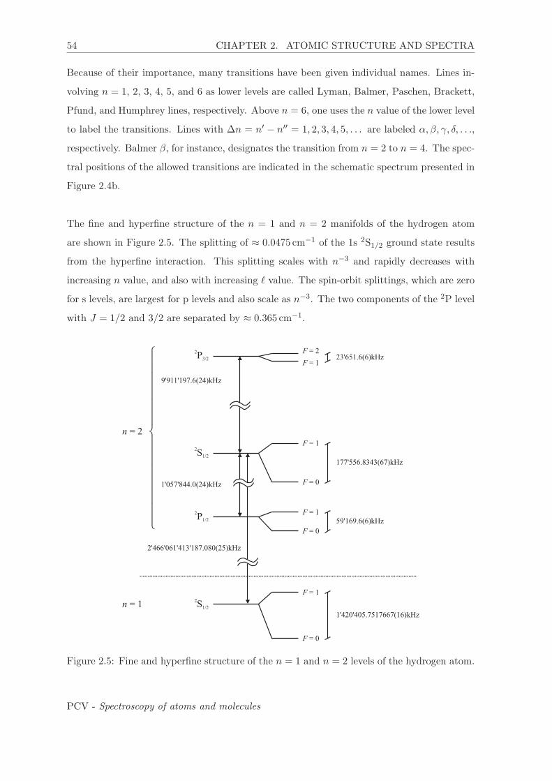
The fine and hyperfine structure of the n = 1 and n = 2 manifolds of the hydrogen atom
are shown in Figure 2.5. The splitting of ≈ 0.0475 cm−1 of the 1s 2S1/2 ground state results
from the hyperfine interaction. This splitting scales with n−3 and rapidly decreases with
increasing n value, and also with increasing � value. The spin-orbit splittings, which are zero
for s levels, are largest for p levels and also scale as n−3. The two components of the 2P level
with J = 1/2 and 3/2 are separated by ≈ 0.365 cm−1.
F = 0
F = 12S1/2
F = 0
F = 12S1/2
F = 0
F = 12P1/2
F = 1
F = 22P3/2 23'651.6(6)kHz
177'556.8343(67)kHz
59'169.6(6)kHz
1'420'405.7517667(16)kHz
9'911'197.6(24)kHz
1'057'844.0(24)kHz
2'466'061'413'187.080(25)kHz
��
��
��
��
��
��
��
n = 2
n = 1
Figure 2.5: Fine and hyperfine structure of the n = 1 and n = 2 levels of the hydrogen atom.
PCV - Spectroscopy of atoms and molecules

2.2. ATOMIC SPECTRA 55
High-resolution spectroscopy of hydrogen-like atoms such as H, He+, Li2+, Be3+ . . . and
their isotopes continues to stimulate methodological and instrumental progress in electronic
spectroscopy. Measurements on ”artificial” hydrogen-like atoms such as positronium (atom
consisting of an electron and a positron), protonium (atom consisting of a proton and an an-
tiproton), antihydrogen (atom consisting of an antiproton and a positron), muonium (atom
consisting of a positive muon μ+ and an electron), antimuonium (atom consisting of a negative
muon μ− and a positron), etc., have the potential of providing new insights into fundamental
physical laws and symmetries and their violations.
2.2.3 Spectra of alkali-metal atoms
A schematic energy level diagram showing the single-photon transitions that can be observed
in the spectra of the alkali-metal atoms is presented in Figure 2.6. The ground-state config-
uration corresponds to a closed-shell rare-gas-atom configuration with a single valence n0s
electron with n0 = 2, 3, 4, 5 and 6 for Li, Na, K, Rb and Cs, respectively. The energetic
positions of these levels can be determined accurately from Equation (2.2). The Laporte
selection rule (Equation (2.72)) restricts the observable single-photon transitions to those
drawn as double-headed arrows in Figure 2.6. Neglecting the fine and hyperfine structures,
their wave numbers can be determined using:
ν =RM
(n′′ − δ�′′)2− RM
(n′ − δ�′)2. (2.74)
s
E/hc
n0s
( +1)sn0
( +2)sn0
p d f
n0p
( +1)pn0
( +1)dn0
( +2)fn0
principal series
sharp series
diffuse series
fundamental series
Figure 2.6: Schematic diagram showing the transitions that can be observed in the single-
photon spectrum of the alkali-metal atoms.
PCV - Spectroscopy of atoms and molecules
56 CHAPTER 2. ATOMIC STRUCTURE AND SPECTRA
The deviation from hydrogenic behavior is accounted for by the �-dependent quantum de-
fects. Transitions from (or to) the lowest energy levels can be grouped in Rydberg series,
which have been called principal, sharp, diffuse and fundamental. Comparing Figure 2.6 with
Figure 2.4, one can see that the principal series of the alkali metal atoms (called principal
because it is observed in absorption and emission) corresponds to the Lyman lines of H, the
diffuse and sharp series to the Balmer lines, and the fundamental series to the Paschen lines.
The quantum defects are only very weakly dependent on the energy. Neglecting this depen-
dence, the quantum defects of the sodium atom are δs ≈ 1.35, δp ≈ 0.86, δd ≈ 0.014, and
δf ≈ 0, so that the lowest-frequency line of the principal series (called the sodium D line
because it is a doublet, see below) lies in the yellow range of the electromagnetic spectrum,
and not in the VUV as Lyman α. The fact that the n0p ← n0s lines of the alkali metal atoms
lie in the visible range of the electromagnetic spectrum makes them readily accessible with
commercial laser sources, and therefore extensively studied and exploited in atomic-physics
experiments.
36MHz16MHz
60MHz
188MHz
1772MHz
17.19 cm = 515.4 GHz-1
16960.9 cm-1
F = 3
F = 2
F = 1F = 0
F = 2
F = 1
F = 2
F = 1
3p P2
3/2
3p P2
1/2
3s S2
1/2
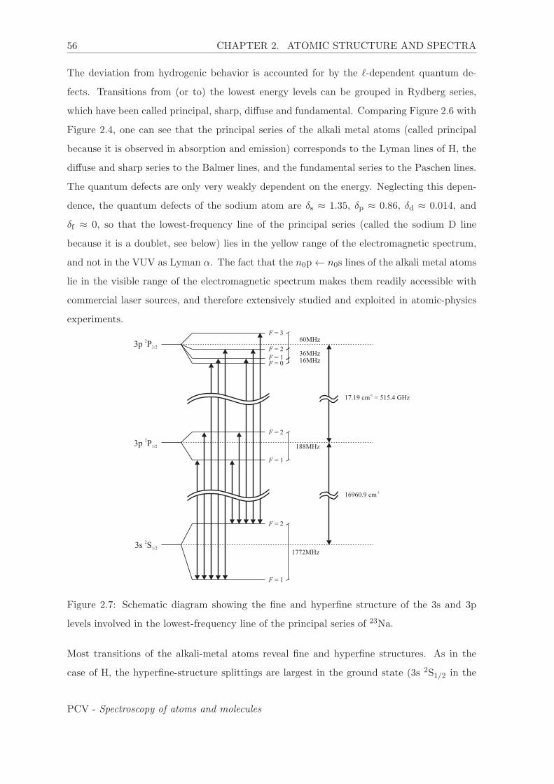
Figure 2.7: Schematic diagram showing the fine and hyperfine structure of the 3s and 3p
levels involved in the lowest-frequency line of the principal series of 23Na.
Most transitions of the alkali-metal atoms reveal fine and hyperfine structures. As in the
case of H, the hyperfine-structure splittings are largest in the ground state (3s 2S1/2 in the
PCV - Spectroscopy of atoms and molecules
2.2. ATOMIC SPECTRA 57
case of Na) and the fine-structure splittings are largest in the lowest-lying p level (3p 2PJ
with J = 1/2, 3/2 in the case of Na). The details of the structure of these two levels of Na
are presented in Figure 2.7. At low resolution, the 3p←3s line appears as a doublet with two
components at 16960.9 cm−1 and 16978.1 cm−1, separated by an interval of 17.2 cm−1 corre-
sponding to the spin-orbit splitting of the 3p state. The second largest splitting (≈ 0.06 cm−1)
in the spectrum arises from the hyperfine splitting of 1772MHz of the 3s state. Finally, split-
tings of less than 200MHz result from the hyperfine structure of the 3p levels.
2.2.4 Spectra of the rare gas atoms
The 1S0 ground state of the rare-gas atoms (Rg=Ne, Ar, Kr and Xe) results from the full-
shell configurations ([. . .](n0p)6 with n0 = 2, 3, 4 and 5 for Ne, Ar, Kr, and Xe, respectively).
Single-photon absorption by electrons in the (n0p)6 orbitals leads to the excitation of J = 1
states of the configurations [. . .](n0p)5(ns)1 and [. . .](n0p)
5(nd)1.
Compared to H and the alkali-metal atoms discussed in the previous examples, the lowest
excited electronic configurations contain two, instead of only one, unpaired electrons, which
leads to both S = 0 and S = 1 states. Moreover, these states form Rydberg series that con-
verge on two closely spaced ionization limits corresponding to the two spin-orbit components
(J+ = 1/2, 3/2) of the 2PJ+ ground state of Rg+, rather than on a single ionization limit, as
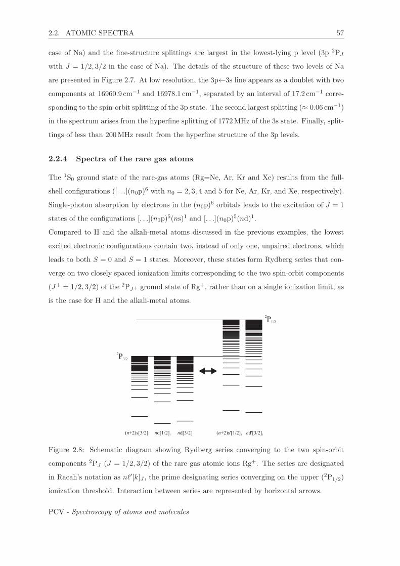
is the case for H and the alkali-metal atoms.
( +2)s[3/2]n 1 nd[3/2]1nd[1/2]1 ( +2)s'[1/2]n 1 nd'[3/2]1
2P1/2
2P3/2
Figure 2.8: Schematic diagram showing Rydberg series converging to the two spin-orbit
components 2PJ (J = 1/2, 3/2) of the rare gas atomic ions Rg+. The series are designated
in Racah’s notation as n�′[k]J , the prime designating series converging on the upper (2P1/2)
ionization threshold. Interaction between series are represented by horizontal arrows.
PCV - Spectroscopy of atoms and molecules
58 CHAPTER 2. ATOMIC STRUCTURE AND SPECTRA
Figure 2.8 depicts schematically the J = 1 Rydberg series of the rare-gas atoms located
below the 2PJ+ (J+ = 1/2, 3/2) ionization thresholds that are optically accessible from the
1S0 ground state. Two angular momentum coupling schemes are used to label these Rydberg
states. The first one corresponds to the familiar LS-coupling scheme discussed in Section 2.1.4
and tends to be realized, if at all, only for the lowest Rydberg states and the lightest atoms.
Five series arise from the optically allowed p→s and p→d transitions, two s series ((n0p)5(ns)1
3P1 and 1P1) and three d series ((n0p)5(nd)1 3D1,
3P1 and 1P1). The second one is a variant
of the jj coupling scheme, and becomes an increasingly exact representation at high n values,
when the spin-orbit coupling in the 2PJ+ ion core becomes stronger than the electrostatic
(including exchange) interaction between the Rydberg and the core electrons. As a result,
the core and Rydberg electrons are decoupled, and J+ becomes a good quantum number
instead of S. In this labeling scheme, the states are designated (2PJ+)n�[k]J , k being the
quantum number resulting from the addition of J+ and �. The five optically accessible J = 1
series are labeled ns[3/2]1, ns′[1/2]1, nd[1/2]1, nd[3/2]1, nd′[3/2]1, the ”prime” being used to
designate the two series converging to the 2P1/2 ionization limit (see Figure 2.8).
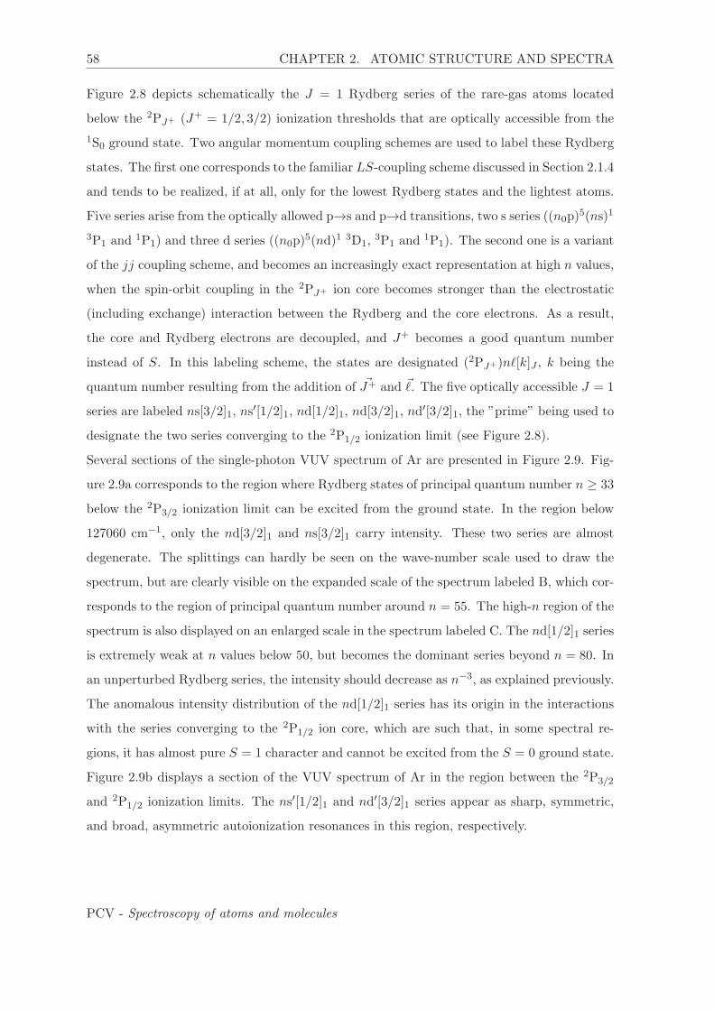
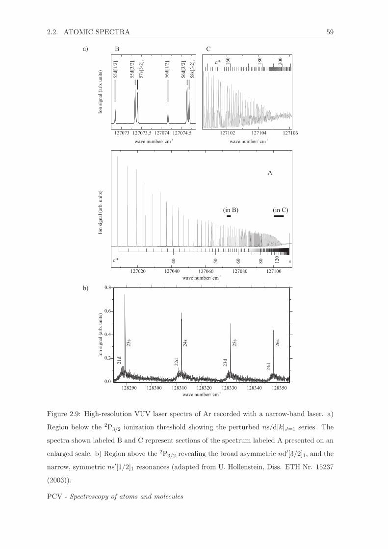
Several sections of the single-photon VUV spectrum of Ar are presented in Figure 2.9. Fig-
ure 2.9a corresponds to the region where Rydberg states of principal quantum number n ≥ 33
below the 2P3/2 ionization limit can be excited from the ground state. In the region below
127060 cm−1, only the nd[3/2]1 and ns[3/2]1 carry intensity. These two series are almost
degenerate. The splittings can hardly be seen on the wave-number scale used to draw the
spectrum, but are clearly visible on the expanded scale of the spectrum labeled B, which cor-
responds to the region of principal quantum number around n = 55. The high-n region of the
spectrum is also displayed on an enlarged scale in the spectrum labeled C. The nd[1/2]1 series
is extremely weak at n values below 50, but becomes the dominant series beyond n = 80. In
an unperturbed Rydberg series, the intensity should decrease as n−3, as explained previously.
The anomalous intensity distribution of the nd[1/2]1 series has its origin in the interactions
with the series converging to the 2P1/2 ion core, which are such that, in some spectral re-
gions, it has almost pure S = 1 character and cannot be excited from the S = 0 ground state.
Figure 2.9b displays a section of the VUV spectrum of Ar in the region between the 2P3/2
and 2P1/2 ionization limits. The ns′[1/2]1 and nd′[3/2]1 series appear as sharp, symmetric,
and broad, asymmetric autoionization resonances in this region, respectively.
PCV - Spectroscopy of atoms and molecules
2.2. ATOMIC SPECTRA 59
40
50
60
80
120
127020 127040 127060 127080 127100
Ion
signal
(arb
.unit
s)
n *
∞
(in B) (in C)
127102 127104 127106
wave number/ cm-1
200
180
160
n *
57s[
3/2
] 1
58s[
3/2
] 1
55d[3
/2] 1
56d[3
/2] 1
55d[1
/2] 1
56d[1
/2] 1
127073 127073.5 127074 127074.5
A
B C
wave number/ cm-1
wave number/ cm-1
Ion
signal
(arb
.unit
s)
a)
128290 128300 128310 128320 128330 128340 128350
0.0
0.2
0.4
0.6
0.8
Ion
signal
(arb
.unit
s)
21d
22d
23d
24d
23s
24s
25s
26s
wave number/ cm-1
b)
Figure 2.9: High-resolution VUV laser spectra of Ar recorded with a narrow-band laser. a)
Region below the 2P3/2 ionization threshold showing the perturbed ns/d[k]J=1 series. The
spectra shown labeled B and C represent sections of the spectrum labeled A presented on an
enlarged scale. b) Region above the 2P3/2 revealing the broad asymmetric nd′[3/2]1, and the
narrow, symmetric ns′[1/2]1 resonances (adapted from U. Hollenstein, Diss. ETH Nr. 15237
(2003)).
PCV - Spectroscopy of atoms and molecules
Related Documents