One-Day Short Course Jianghua He, Ph.D. Associate Professor, Department of Biostatistics University of Kansas Medical Center [email protected] Survival Analysis

Welcome message from author
This document is posted to help you gain knowledge. Please leave a comment to let me know what you think about it! Share it to your friends and learn new things together.
Transcript

One-Day Short Course
Jianghua He, Ph.D. Associate Professor, Department of Biostatistics University of Kansas Medical Center [email protected]
Survival Analysis
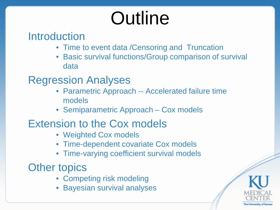
Outline Introduction
• Time to event data /Censoring and Truncation • Basic survival functions/Group comparison of survival
data
Regression Analyses • Parametric Approach -- Accelerated failure time
models • Semiparametric Approach – Cox models
Extension to the Cox models • Weighted Cox models • Time-dependent covariate Cox models • Time-varying coefficient survival models
Other topics • Competing risk modeling • Bayesian survival analyses
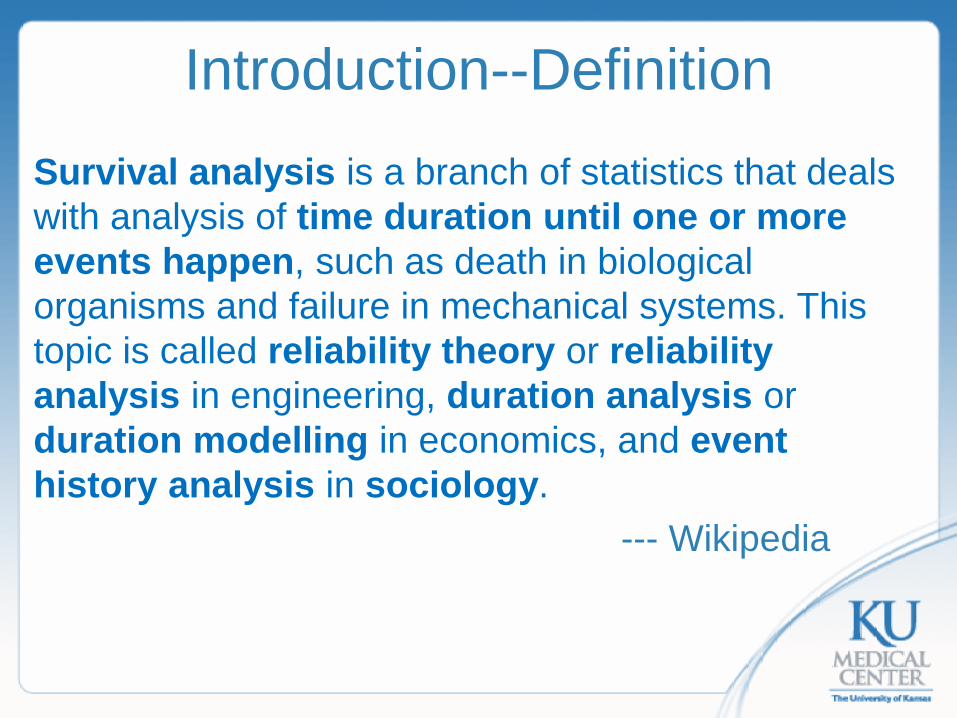
Introduction--Definition Survival analysis is a branch of statistics that deals with analysis of time duration until one or more events happen, such as death in biological organisms and failure in mechanical systems. This topic is called reliability theory or reliability analysis in engineering, duration analysis or duration modelling in economics, and event history analysis in sociology. --- Wikipedia

Introduction--Definition With survival analysis, we can try to answer questions such as: What are the 5-year or 10-year survival rates for
certain diseases after diagnosis? What are the risk factors that contribute to the risk of
events? Does the new treatment reduce the risk (increase the
survival rate) compared to the placebo or old treatment?
Can multiple causes of death or failure be taken into account?
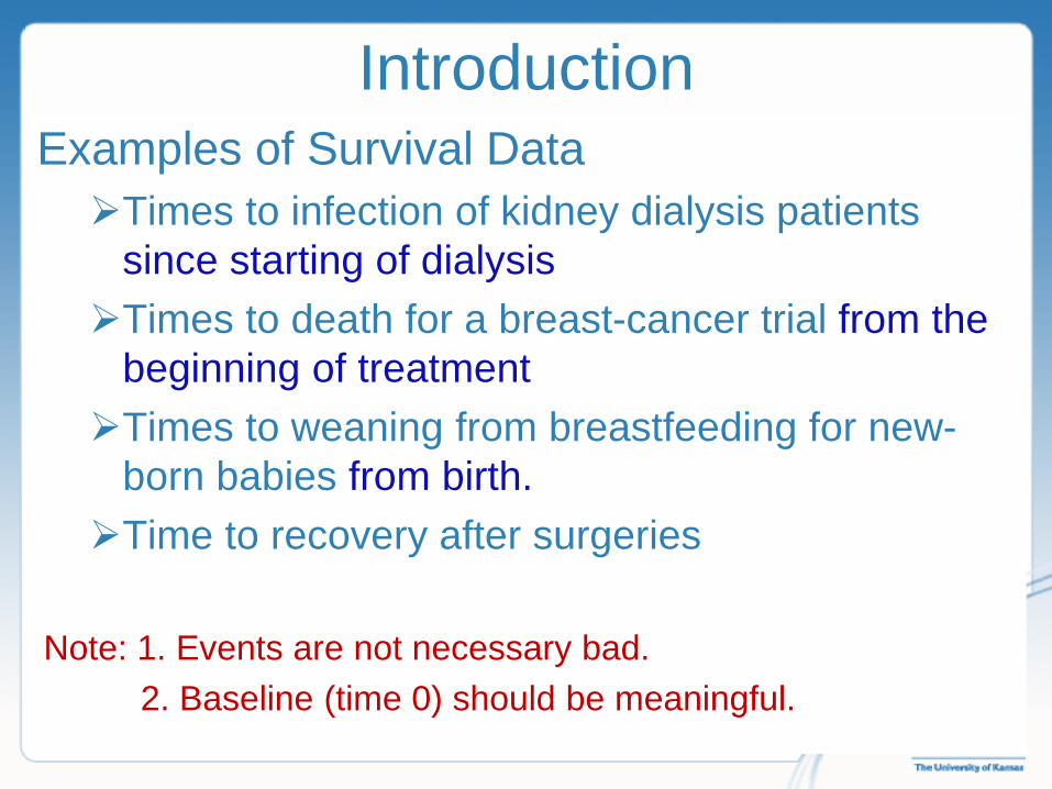
Introduction Examples of Survival Data Times to infection of kidney dialysis patients
since starting of dialysis Times to death for a breast-cancer trial from the
beginning of treatment Times to weaning from breastfeeding for new-
born babies from birth. Time to recovery after surgeries
Note: 1. Events are not necessary bad. 2. Baseline (time 0) should be meaningful.
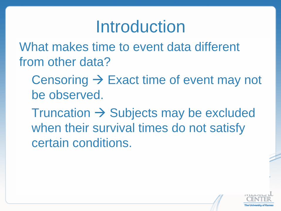
Introduction What makes time to event data different from other data?
Censoring Exact time of event may not be observed. Truncation Subjects may be excluded when their survival times do not satisfy certain conditions.

Introduction---Censoring Assume there is a study of cancer patients’ survival after a new cancer treatment. The following plot shows a typical outcome of the study
Reasons of censoring could be: dropout, death unrelated to the specific cancer, end of follow-up, etc.
Observed event time
Censored (right) event time
Time 0 may not be the same calendar time for subjects due to the enrollment process
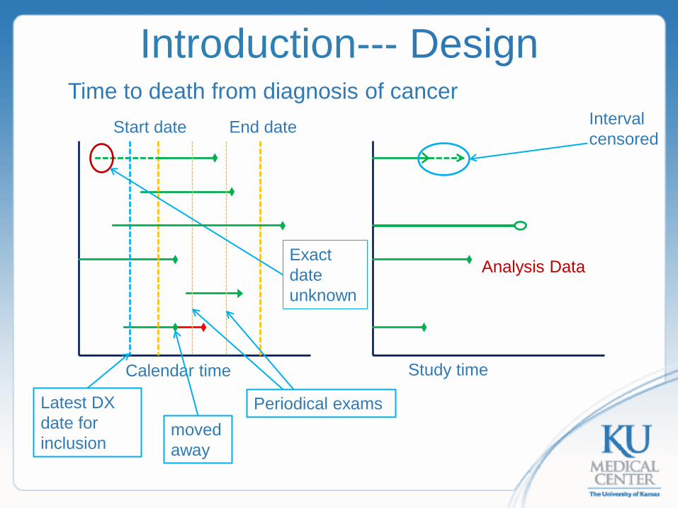
Introduction--- Design Time to death from diagnosis of cancer
Latest DX date for inclusion
Calendar time
Start date End date
Periodical exams
Exact date unknown
moved away
Study time
Analysis Data
Interval censored
Introduction---Censoring Sometimes, an event is not observed but is known to happen after certain time point (right censored), or before certain time point (left-censored), or during a certain time period (interval-censored). • Linear models cannot handle censored observations
directly and have to exclude all unobserved observations or use computed or censored observations. The uniqueness of survival analysis is that it can handle censored observations directly.
• Logistic regression doesn’t take event time into consideration and will lose some useful information. The results may be biased if we treat censored cases as non-events or exclude them from analyses.
Introduction---Censoring In reality, right censoring is the most commonly seen situation. The observed survival time 𝑋𝑋 = min (𝑇𝑇, 𝐶𝐶 ), where 𝐶𝐶 is the censoring time. Another important element is the censoring indicator 𝛿𝛿 = 1 event if X =T, otherwise 𝛿𝛿 = 0(censored). Data: (𝑥𝑥1, 𝛿𝛿 1), (𝑥𝑥2, 𝛿𝛿 2), (𝑥𝑥3, 𝛿𝛿 3),…, (𝑥𝑥𝑛𝑛, 𝛿𝛿 𝑛𝑛) For interval censored data, both the upper limit and lower limit will be provided.
Introduction---Censoring Noninformative/Independent Censoring Time to censoring 𝐶𝐶 can be considered another time to event variable. Independent censoring means time to event of interest 𝑇𝑇 and 𝐶𝐶 are independent. Knowing the censoring times provide no extra information about the potential event times besides what is already known (conditional independence). Most of the survival analyses methods are based on this assumption. However, this assumption cannot be tested within a given data (Identifiability Dilemma).

Introduction---Censoring Noninformative/Independent Censoring Independence assumption is often based clinical consideration. For example, time to cancer death and censoring due to traffic accidents can be considered as independent.In a clinical trial, censoring due to dropouts unrelated to disease severity can be considered independent. Sometimes patients who are doing worse are more likely to drop out (they might think the treatment is harmful), sometimes it is the other way around (less severe patients are less motivated to follow the protocol). These types of censoring should not be considered as independent.
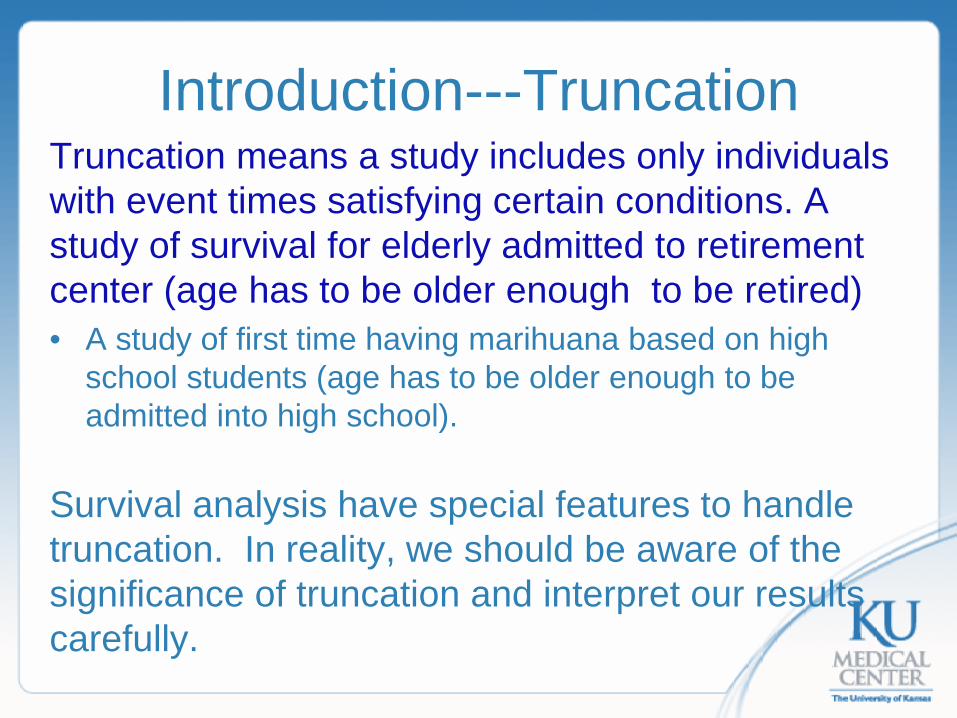
Introduction---Truncation Truncation means a study includes only individuals with event times satisfying certain conditions. A study of survival for elderly admitted to retirement center (age has to be older enough to be retired) • A study of first time having marihuana based on high
school students (age has to be older enough to be admitted into high school).
Survival analysis have special features to handle truncation. In reality, we should be aware of the significance of truncation and interpret our results carefully.
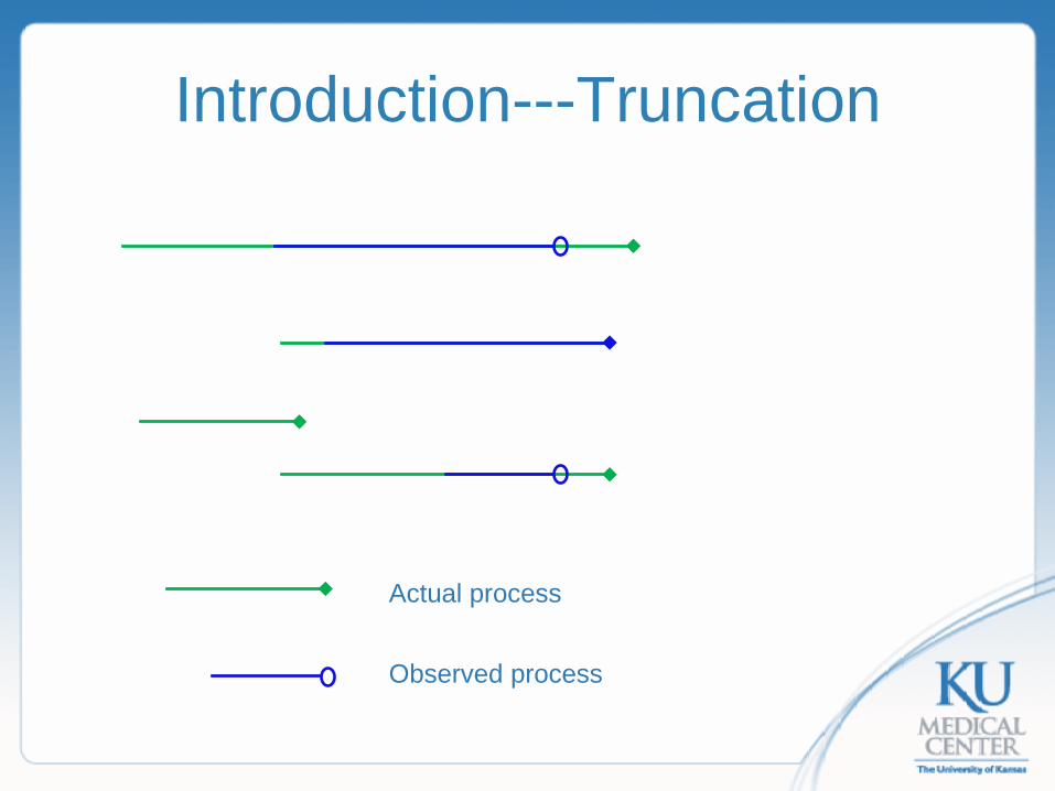
Introduction---Truncation
Actual process
Observed process
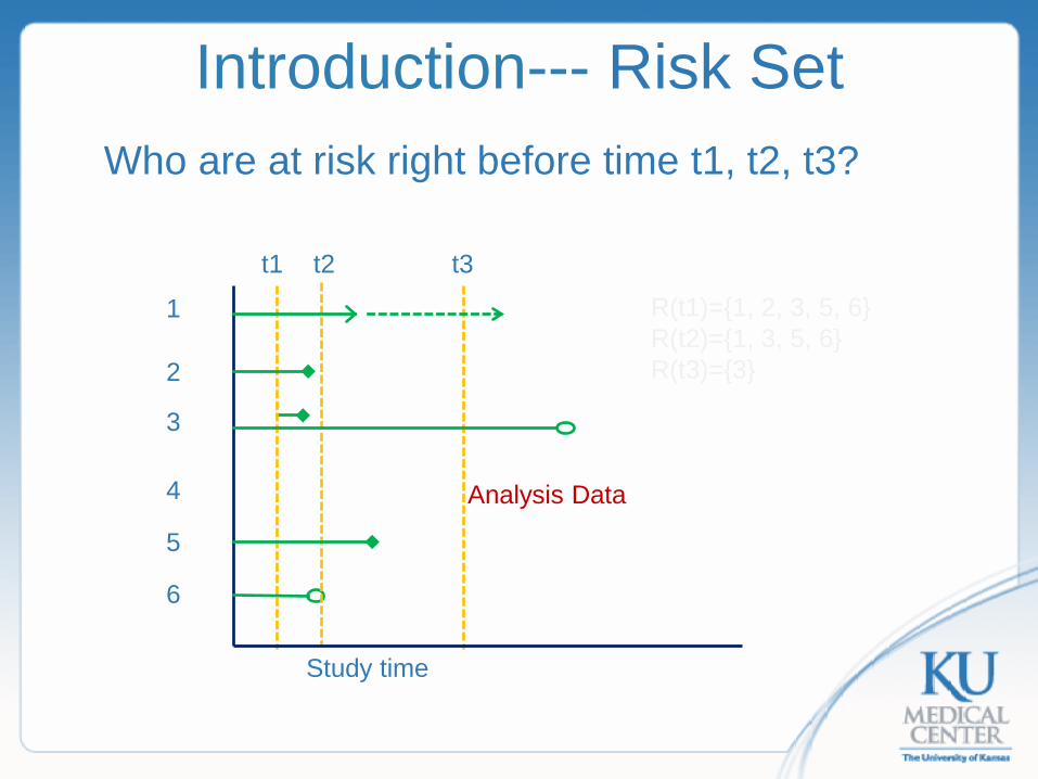
Introduction--- Risk Set Who are at risk right before time t1, t2, t3?
Study time
Analysis Data
1
2
3
4
6
t1 t2 t3
R(t1)={1, 2, 3, 5, 6} R(t2)={1, 3, 5, 6} R(t3)={3}
5
Introduction---Examples Some course materials are based on the following textbooks. Survival Analysis: Techniques for Censored and Truncated Data, 2nd ed., by J. P. Klein and M. L. Moeschberger Data and SAS program codes are available online http://www.ats.ucla.edu/stat/examples/sakm/ Applied Survival Analysis 2nd ed., by D.W. Hosmer, S. Lemeshow, and S. May. Data and program codes (SAS, STATA, SPSS) http://www.ats.ucla.edu/stat/examples/asa2/default.htm www.umass.edu/statdata/statdata/stat-survival.html

Introduction---Examples Kidney Dialysis Purpose: To assess the impact of catheter placement methods on the time to first exit-site infection (in months) in patients with renal insufficiency.
Treatment: Surgical placement (n=43) vs. Percutaneous placement (76).
Many right censored cases.
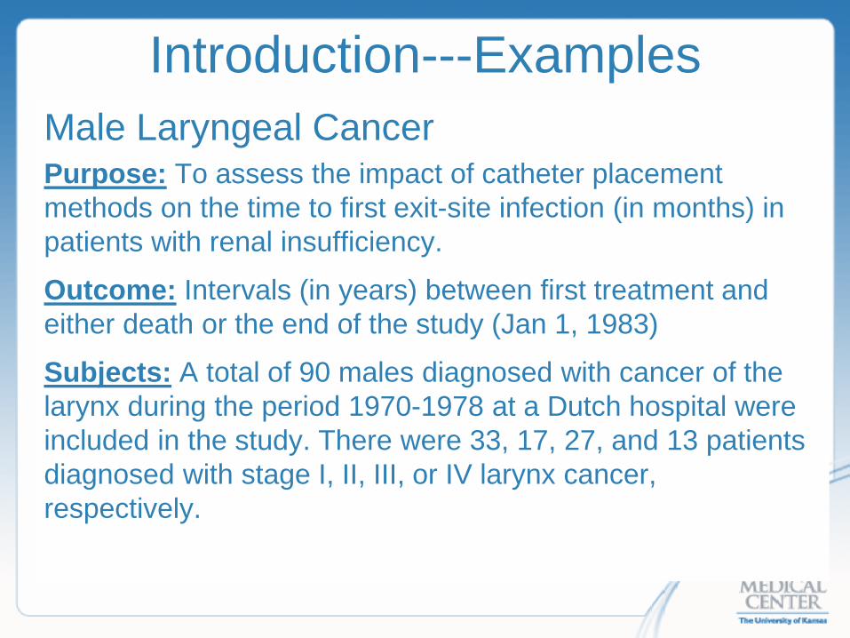
Introduction---Examples Male Laryngeal Cancer Purpose: To assess the impact of catheter placement methods on the time to first exit-site infection (in months) in patients with renal insufficiency.
Outcome: Intervals (in years) between first treatment and either death or the end of the study (Jan 1, 1983)
Subjects: A total of 90 males diagnosed with cancer of the larynx during the period 1970-1978 at a Dutch hospital were included in the study. There were 33, 17, 27, and 13 patients diagnosed with stage I, II, III, or IV larynx cancer, respectively.
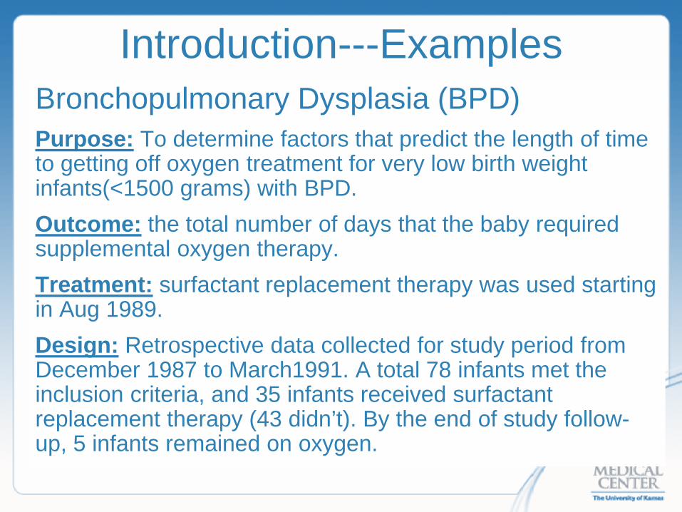
Introduction---Examples Bronchopulmonary Dysplasia (BPD) Purpose: To determine factors that predict the length of time to getting off oxygen treatment for very low birth weight infants(<1500 grams) with BPD. Outcome: the total number of days that the baby required supplemental oxygen therapy. Treatment: surfactant replacement therapy was used starting in Aug 1989. Design: Retrospective data collected for study period from December 1987 to March1991. A total 78 infants met the inclusion criteria, and 35 infants received surfactant replacement therapy (43 didn’t). By the end of study follow-up, 5 infants remained on oxygen.

Introduction---Examples Framingham Heart Study A joint project of the National Heart, Lung and Blood Institute and Boston University to study risk factors of heart diseases. The researchers recruited 5,209 men and women between the ages of 30 and 62 from the town of Framingham, Massachusetts. Since 1948, the subjects return to the study every two years for a detailed medical history, physical examination, and laboratory tests.

Introduction---Basic Functions Continuous Survival Time X Cumulative distribution function 𝐹𝐹(𝑥𝑥) = 𝑃𝑃(𝑋𝑋 ≤ 𝑥𝑥) Probability density function 𝑓𝑓 𝑥𝑥 = 𝑑𝑑𝑑𝑑 𝑥𝑥
𝑑𝑑𝑥𝑥= lim
∆𝑥𝑥→0𝑃𝑃(𝑥𝑥≤𝑋𝑋≤𝑥𝑥+∆𝑥𝑥)
∆𝑥𝑥
Survival function: 0 ≤ 𝑆𝑆 𝑥𝑥 ≤ 1 𝑆𝑆 𝑥𝑥 = 𝑃𝑃 𝑋𝑋 > 𝑥𝑥 = 1 − 𝐹𝐹 𝑥𝑥
= � 𝑓𝑓 𝑥𝑥 𝑑𝑑𝑥𝑥∞
𝑥𝑥
Thus
𝑓𝑓 𝑥𝑥 = − 𝑑𝑑𝑆𝑆 𝑥𝑥𝑑𝑑𝑥𝑥
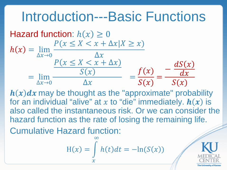
Hazard function: ℎ 𝑥𝑥 ≥ 0
ℎ 𝑥𝑥 = lim∆𝑥𝑥→0
𝑃𝑃(𝑥𝑥 ≤ 𝑋𝑋 < 𝑥𝑥 + ∆𝑥𝑥|𝑋𝑋 ≥ 𝑥𝑥)∆𝑥𝑥
= lim∆𝑥𝑥→0
𝑃𝑃 𝑥𝑥 ≤ 𝑋𝑋 < 𝑥𝑥 + ∆𝑥𝑥𝑆𝑆 𝑥𝑥∆𝑥𝑥
=𝑓𝑓(𝑥𝑥)𝑆𝑆(𝑥𝑥)
=− 𝑑𝑑𝑆𝑆 𝑥𝑥
𝑑𝑑𝑥𝑥𝑆𝑆(𝑥𝑥)
𝒉𝒉 𝒙𝒙 𝒅𝒅𝒙𝒙 may be thought as the "approximate" probability for an individual “alive” at 𝑥𝑥 to “die” immediately. 𝒉𝒉 𝒙𝒙 is also called the instantaneous risk. Or we can consider the hazard function as the rate of losing the remaining life. Cumulative Hazard function:
H 𝑥𝑥 = � ℎ 𝑡𝑡 𝑑𝑑𝑡𝑡∞
𝑥𝑥
= −ln (𝑆𝑆 𝑥𝑥 )
Introduction---Basic Functions
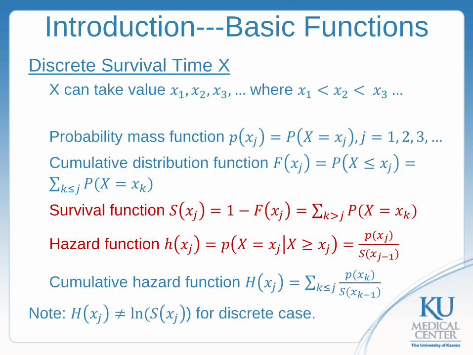
Introduction---Basic Functions Discrete Survival Time X
X can take value 𝑥𝑥1, 𝑥𝑥2, 𝑥𝑥3, … where 𝑥𝑥1 < 𝑥𝑥2 < 𝑥𝑥3 … Probability mass function 𝑝𝑝 𝑥𝑥𝑗𝑗 = 𝑃𝑃 𝑋𝑋 = 𝑥𝑥𝑗𝑗 , 𝑗𝑗 = 1, 2, 3, … Cumulative distribution function 𝐹𝐹 𝑥𝑥𝑗𝑗 = 𝑃𝑃 𝑋𝑋 ≤ 𝑥𝑥𝑗𝑗 =∑ 𝑃𝑃(𝑋𝑋 = 𝑥𝑥𝑘𝑘)𝑘𝑘≤𝑗𝑗
Survival function 𝑆𝑆 𝑥𝑥𝑗𝑗 = 1 − 𝐹𝐹 𝑥𝑥𝑗𝑗 = ∑ 𝑃𝑃(𝑋𝑋 = 𝑥𝑥𝑘𝑘)𝑘𝑘>𝑗𝑗
Hazard function ℎ 𝑥𝑥𝑗𝑗 = 𝑝𝑝 𝑋𝑋 = 𝑥𝑥𝑗𝑗 𝑋𝑋 ≥ 𝑥𝑥𝑗𝑗 = 𝑝𝑝(𝑥𝑥𝑗𝑗)𝑆𝑆(𝑥𝑥𝑗𝑗−1)
Cumulative hazard function 𝐻𝐻 𝑥𝑥𝑗𝑗 = ∑ 𝑝𝑝(𝑥𝑥𝑘𝑘)𝑆𝑆(𝑥𝑥𝑘𝑘−1)𝑘𝑘≤𝑗𝑗
Note: 𝐻𝐻 𝑥𝑥𝑗𝑗 ≠ ln (𝑆𝑆 𝑥𝑥𝑗𝑗 ) for discrete case.
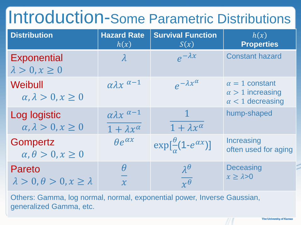
Distribution Hazard Rate ℎ 𝑥𝑥
Survival Function 𝑆𝑆 𝑥𝑥
ℎ 𝑥𝑥 Properties
Exponential 𝜆𝜆 > 0, 𝑥𝑥 ≥ 0
𝜆𝜆 𝑒𝑒−𝜆𝜆𝑥𝑥 Constant hazard
Weibull 𝛼𝛼, 𝜆𝜆 > 0, 𝑥𝑥 ≥ 0
𝛼𝛼𝜆𝜆𝑥𝑥 𝛼𝛼−1 𝑒𝑒−𝜆𝜆𝑥𝑥𝛼𝛼 𝛼𝛼 = 1 constant 𝛼𝛼 > 1 increasing 𝛼𝛼 < 1 decreasing
Log logistic 𝛼𝛼, 𝜆𝜆 > 0, 𝑥𝑥 ≥ 0
𝛼𝛼𝜆𝜆𝑥𝑥 𝛼𝛼−1
1 + 𝜆𝜆𝑥𝑥𝛼𝛼
11 + 𝜆𝜆𝑥𝑥𝛼𝛼
hump-shaped
Gompertz 𝛼𝛼,𝜃𝜃 > 0, 𝑥𝑥 ≥ 0
𝜃𝜃𝑒𝑒𝛼𝛼𝑥𝑥 exp [𝜃𝜃𝛼𝛼(1-𝑒𝑒𝛼𝛼𝑥𝑥)] Increasing
often used for aging
Pareto 𝜆𝜆 > 0,𝜃𝜃 > 0, 𝑥𝑥 ≥ 𝜆𝜆
𝜃𝜃𝑥𝑥
𝜆𝜆𝜃𝜃
𝑥𝑥𝜃𝜃
Deceasing 𝑥𝑥 ≥ 𝜆𝜆>0
Others: Gamma, log normal, normal, exponential power, Inverse Gaussian, generalized Gamma, etc.
Introduction-Some Parametric Distributions
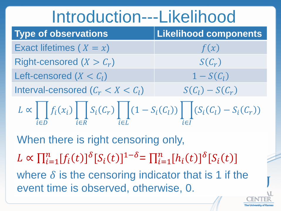
Introduction---Likelihood
𝐿𝐿 ∝�𝑓𝑓𝑖𝑖 𝑥𝑥𝑖𝑖𝑖𝑖∈𝐷𝐷
�𝑆𝑆𝑖𝑖 𝐶𝐶𝑟𝑟𝑖𝑖∈𝑅𝑅
�(1 − 𝑆𝑆𝑖𝑖 𝐶𝐶𝑙𝑙 )𝑖𝑖∈𝐿𝐿
�(𝑆𝑆𝑖𝑖 𝐶𝐶𝑙𝑙 − 𝑆𝑆𝑖𝑖 𝐶𝐶𝑟𝑟 )𝑖𝑖∈𝐼𝐼
When there is right censoring only,
𝐿𝐿 ∝ ∏ [𝑓𝑓𝑖𝑖 𝑡𝑡 ]𝛿𝛿[𝑆𝑆𝑖𝑖 𝑡𝑡 ]1−𝛿𝛿𝑛𝑛𝑖𝑖=1 = ∏ [ℎ𝑖𝑖 𝑡𝑡 ]𝛿𝛿[𝑆𝑆𝑖𝑖 𝑡𝑡 ]𝑛𝑛
𝑖𝑖=1
where 𝛿𝛿 is the censoring indicator that is 1 if the event time is observed, otherwise, 0.
Type of observations Likelihood components Exact lifetimes ( 𝑋𝑋 = 𝑥𝑥) 𝑓𝑓 𝑥𝑥 Right-censored (𝑋𝑋 > 𝐶𝐶𝑟𝑟) 𝑆𝑆 𝐶𝐶𝑟𝑟 Left-censored (𝑋𝑋 < 𝐶𝐶𝑙𝑙) 1 − 𝑆𝑆 𝐶𝐶𝑙𝑙 Interval-censored (𝐶𝐶𝑟𝑟 < 𝑋𝑋 < 𝐶𝐶𝑙𝑙) 𝑆𝑆 𝐶𝐶𝑙𝑙 − 𝑆𝑆 𝐶𝐶𝑟𝑟
Introduction---Likelihood
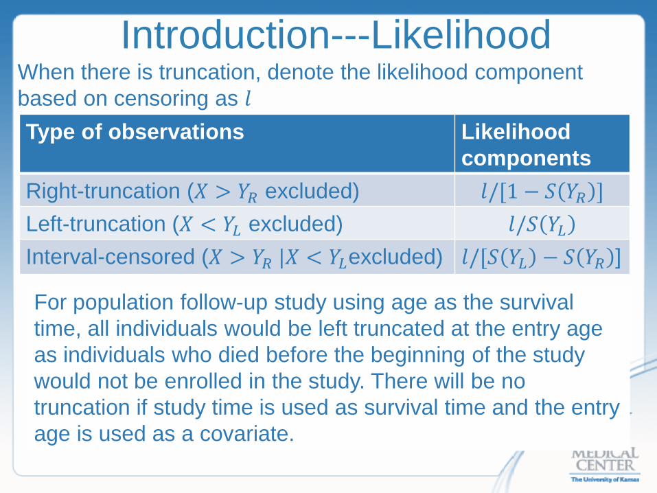
Type of observations Likelihood components
Right-truncation (𝑋𝑋 > 𝑌𝑌𝑅𝑅 excluded) 𝑙𝑙/[1 − 𝑆𝑆 𝑌𝑌𝑅𝑅 ] Left-truncation (𝑋𝑋 < 𝑌𝑌𝐿𝐿 excluded) 𝑙𝑙/𝑆𝑆 𝑌𝑌𝐿𝐿 Interval-censored (𝑋𝑋 > 𝑌𝑌𝑅𝑅 |𝑋𝑋 < 𝑌𝑌𝐿𝐿excluded) 𝑙𝑙/[𝑆𝑆 𝑌𝑌𝐿𝐿 − 𝑆𝑆 𝑌𝑌𝑅𝑅 ]
When there is truncation, denote the likelihood component based on censoring as 𝑙𝑙
For population follow-up study using age as the survival time, all individuals would be left truncated at the entry age as individuals who died before the beginning of the study would not be enrolled in the study. There will be no truncation if study time is used as survival time and the entry age is used as a covariate.
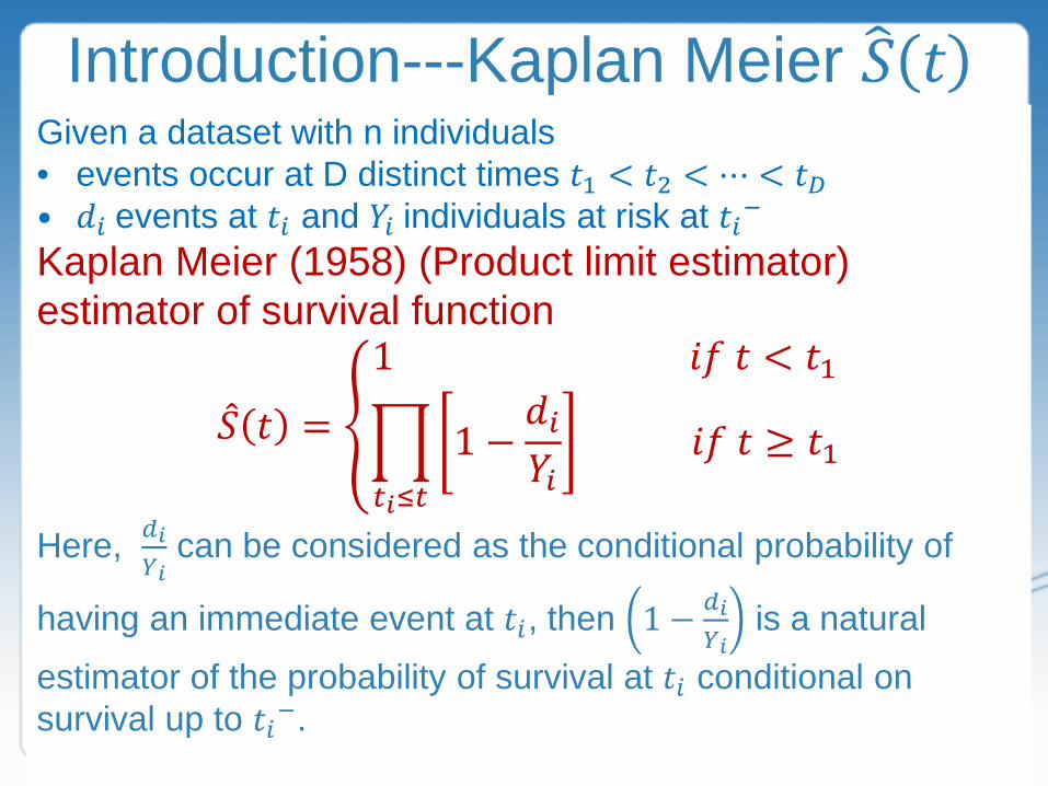
Introduction---Kaplan Meier 𝑆𝑆� 𝑡𝑡 Given a dataset with n individuals • events occur at D distinct times 𝑡𝑡1 < 𝑡𝑡2 < ⋯ < 𝑡𝑡𝐷𝐷 • 𝑑𝑑𝑖𝑖 events at 𝑡𝑡𝑖𝑖 and 𝑌𝑌𝑖𝑖 individuals at risk at 𝑡𝑡𝑖𝑖− Kaplan Meier (1958) (Product limit estimator) estimator of survival function
�̂�𝑆 𝑡𝑡 = �
1 𝑖𝑖𝑓𝑓 𝑡𝑡 < 𝑡𝑡1
� 1 −𝑑𝑑𝑖𝑖𝑌𝑌𝑖𝑖𝑡𝑡𝑖𝑖≤𝑡𝑡
𝑖𝑖𝑓𝑓 𝑡𝑡 ≥ 𝑡𝑡1
Here, 𝑑𝑑𝑖𝑖𝑌𝑌𝑖𝑖
can be considered as the conditional probability of
having an immediate event at 𝑡𝑡𝑖𝑖, then 1 − 𝑑𝑑𝑖𝑖𝑌𝑌𝑖𝑖
is a natural
estimator of the probability of survival at 𝑡𝑡𝑖𝑖 conditional on survival up to 𝑡𝑡𝑖𝑖−.
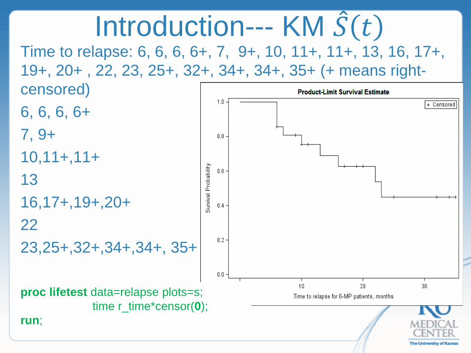
Time to relapse: 6, 6, 6, 6+, 7, 9+, 10, 11+, 11+, 13, 16, 17+, 19+, 20+ , 22, 23, 25+, 32+, 34+, 34+, 35+ (+ means right-censored) 6, 6, 6, 6+ 7, 9+ 10,11+,11+ 13 16,17+,19+,20+ 22 23,25+,32+,34+,34+, 35+
Introduction--- KM �̂�𝑆 𝑡𝑡
proc lifetest data=relapse plots=s; time r_time*censor(0); run;
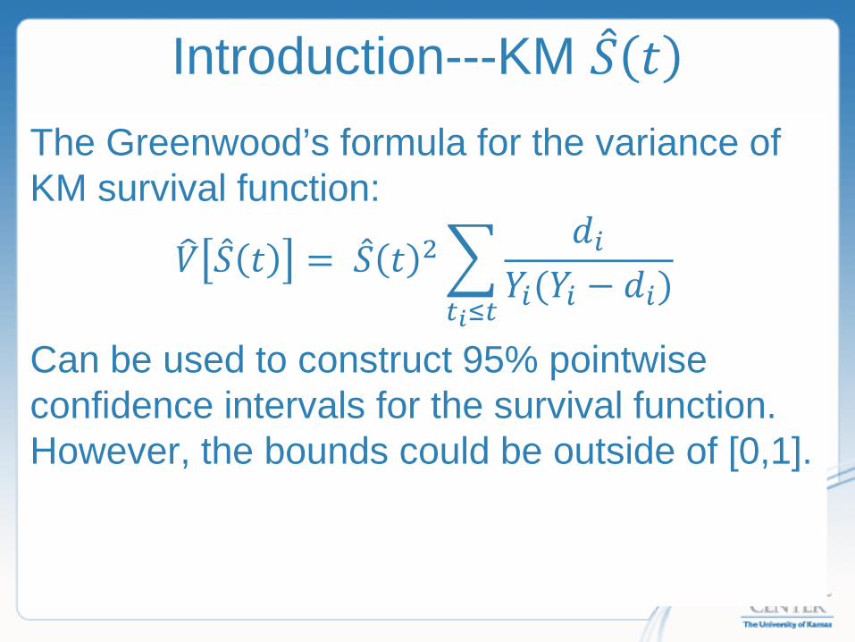
Introduction---KM �̂�𝑆 𝑡𝑡 The Greenwood’s formula for the variance of KM survival function:
𝑉𝑉� �̂�𝑆 𝑡𝑡 = �̂�𝑆 𝑡𝑡 2�𝑑𝑑𝑖𝑖
𝑌𝑌𝑖𝑖(𝑌𝑌𝑖𝑖 − 𝑑𝑑𝑖𝑖)𝑡𝑡𝑖𝑖≤𝑡𝑡
Can be used to construct 95% pointwise confidence intervals for the survival function. However, the bounds could be outside of [0,1].

Introduction---Survival Function Other point-wise confidence intervals for survival functions and these CIs are bounded within 0-1.
Log-log transformation: ln(−ln[�̂�𝑆 𝑡𝑡0)] Log transformation:ln[�̂�𝑆 𝑡𝑡0 ]
Logit transformation:ln{ �̂�𝑆 𝑡𝑡01−�̂�𝑆 𝑡𝑡0 }
Arcsine square-root transformation: arcsin[ �̂�𝑆 𝑡𝑡0 ] PROC LIFETEST < options > ; CONFTYPE= LINEAR/ASINSQRT/LOGLOG/LOG/LOGIT; Confidence Bands (apply to the entire time range) CONFBAND=ALL (both EP and HW) EP (equal-precision CBs) HW (Hall-Wellner CBs)

Introduction---Survival Function Pointwise Confidence Intervals and Confidence Bands
SAS automatically truncate all bounds to be within 0-1
EP CBs
HW CBs CIs

Introduction---Survival Function Pointwise Confidence Intervals and Confidence Bands
Note: Lower Confidence Bands are not monotonic
EP CBs
HW CBs CIs

Introduction---Survival Function Pointwise Confidence Intervals and Confidence Bands
Note: Lower Confidence Bands are not monotonic
EP CBs
HW CBs CIs
Introduction---Survival Function Life table A life table is a summary of the survival data grouped into convenient intervals. Life table is often used in actuarial for life insurance. This approach is much more convenient than K-M estimator when the sample size is very large. Intervals 𝐼𝐼1, 𝐼𝐼2, … , 𝐼𝐼𝑘𝑘 and the corresponding knots: 𝑡𝑡0, 𝑡𝑡1, 𝑡𝑡2 … , 𝑡𝑡𝑘𝑘.

Introduction---Survival Function Life table An example of cost of group life insurance for adults of AIChE Group Source: http://www.aicheinsurance.com/sites/aiche/Pages/GroupTerm-CoverageLimitsandRates.aspx

Life table
Ii=(ti-1, ti] Risk set at ti-1- Events
in Ii Censored cases in Ii
P(t>ti|t> ti-1)
𝐼𝐼1 𝑛𝑛0 = 𝑛𝑛 𝑑𝑑1 𝑐𝑐1 1 −𝑑𝑑1
(𝑛𝑛0 −𝑐𝑐12 )
𝐼𝐼2 𝑛𝑛1 = 𝑛𝑛 − 𝑑𝑑1 − 𝑐𝑐1 𝑑𝑑2 𝑐𝑐2 1 −𝑑𝑑2
(𝑛𝑛1 −𝑐𝑐22 )
… … … … …
𝐼𝐼𝑘𝑘 𝑛𝑛𝑘𝑘−1 = 𝑛𝑛 −�(𝑑𝑑𝑗𝑗 + 𝑐𝑐𝑗𝑗)𝑘𝑘−1
𝑗𝑗=1
𝑑𝑑𝑘𝑘 𝑐𝑐𝑘𝑘 1 −𝑑𝑑𝑘𝑘
(𝑛𝑛𝑘𝑘−1 −𝑐𝑐𝑘𝑘2 )
Survival Function is in a similar form of KM estimator
𝑆𝑆� 𝑡𝑡 = � 1 −𝑑𝑑𝑖𝑖
(𝑛𝑛𝑖𝑖−1 −𝑐𝑐𝑖𝑖2)𝑡𝑡𝑖𝑖≤𝑡𝑡

Introduction---Survival Function Life table proc lifetest data=bpd method=lt intervals=(0 to 750 by 50) plots=s; time ondays*censor(0) ; strata surfact; run;

Introduction Nelson-Aalen estimator of cumulative hazard function
𝐻𝐻� 𝑡𝑡 = �0 𝑖𝑖𝑓𝑓 𝑡𝑡 < 𝑡𝑡1
�𝑑𝑑𝑖𝑖𝑌𝑌𝑖𝑖𝑡𝑡𝑖𝑖≤𝑡𝑡
𝑖𝑖𝑓𝑓 𝑡𝑡 ≥ 𝑡𝑡1
Based on this estimator, an alternative estimator of the survival function is given by
�̃�𝑆 𝑡𝑡 = exp [−𝐻𝐻� 𝑡𝑡 ] This estimate is equal or greater than the K-M estimate. Note: The N-A estimator 𝐻𝐻� 𝑡𝑡 is the first term in a Taylor series expansion of -𝑙𝑙𝑛𝑛 �̂�𝑆 𝑡𝑡 = 𝐻𝐻� 𝑡𝑡 .
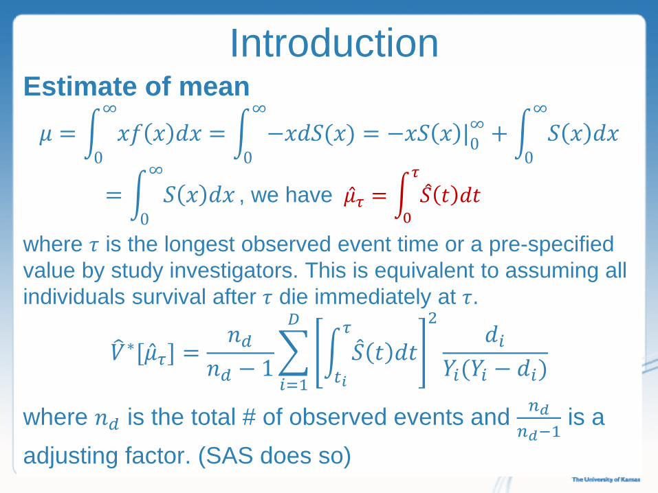
Introduction Estimate of mean 𝜇𝜇 = � 𝑥𝑥𝑓𝑓 𝑥𝑥 𝑑𝑑𝑥𝑥
∞
0= � −𝑥𝑥𝑑𝑑𝑆𝑆(𝑥𝑥)
∞
0= −𝑥𝑥𝑆𝑆 𝑥𝑥 |0
∞ + � 𝑆𝑆 𝑥𝑥 𝑑𝑑𝑥𝑥∞
0
= � 𝑆𝑆 𝑥𝑥 𝑑𝑑𝑥𝑥∞
0, we have �̂�𝜇𝜏𝜏 = � 𝑆𝑆 𝑡𝑡 𝑑𝑑𝑡𝑡
𝜏𝜏
0
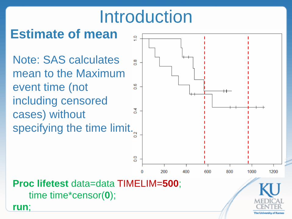
where 𝜏𝜏 is the longest observed event time or a pre-specified value by study investigators. This is equivalent to assuming all individuals survival after 𝜏𝜏 die immediately at 𝜏𝜏.
𝑉𝑉�∗[�̂�𝜇𝜏𝜏] =𝑛𝑛𝑑𝑑
𝑛𝑛𝑑𝑑 − 1� � �̂�𝑆 𝑡𝑡 𝑑𝑑𝑡𝑡
𝜏𝜏
𝑡𝑡𝑖𝑖
2𝑑𝑑𝑖𝑖
𝑌𝑌𝑖𝑖(𝑌𝑌𝑖𝑖 − 𝑑𝑑𝑖𝑖)
𝐷𝐷
𝑖𝑖=1
where 𝑛𝑛𝑑𝑑 is the total # of observed events and 𝑛𝑛𝑑𝑑𝑛𝑛𝑑𝑑−1
is a adjusting factor. (SAS does so)

Introduction Estimates of mean
�̂�𝜇𝜏𝜏 = � �̂�𝑆 𝑡𝑡 𝑑𝑑𝑡𝑡𝜏𝜏
0
this is equivalent to the area under the survival curve up to 𝜏𝜏. When we compare means among groups, make sure the same 𝜏𝜏 is applied to all groups for a fair comparison, and 𝜏𝜏 is appropriate for all groups (𝜏𝜏 < max𝑖𝑖 (𝑡𝑡𝑖𝑖𝑗𝑗) for ∀ 𝑖𝑖 ).
Introduction Estimate of mean
Proc lifetest data=data TIMELIM=500; time time*censor(0); run;
Note: SAS calculates mean to the Maximum event time (not including censored cases) without specifying the time limit.
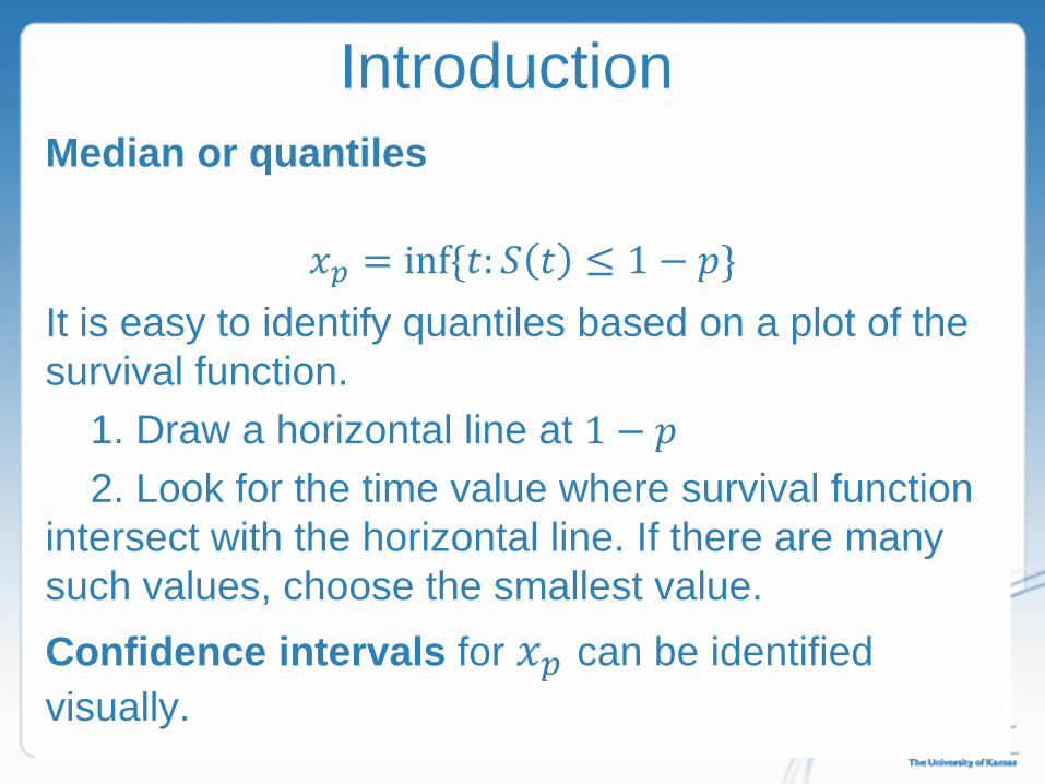
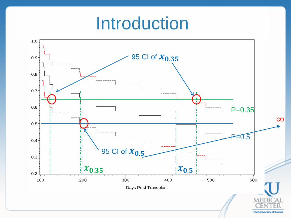
Introduction Median or quantiles
𝑥𝑥𝑝𝑝 = inf{𝑡𝑡: 𝑆𝑆 𝑡𝑡 ≤ 1 − 𝑝𝑝} It is easy to identify quantiles based on a plot of the survival function. 1. Draw a horizontal line at 1 − 𝑝𝑝 2. Look for the time value where survival function intersect with the horizontal line. If there are many such values, choose the smallest value. Confidence intervals for 𝑥𝑥𝑝𝑝 can be identified visually.
'
0.2
0.3
0.4
0.5
0.6
0.7
0.8
0.9
1.0
Days Post Transplant
100 200 300 400 500 600
CIs for quantiles
P=0.5
P=0.35
𝒙𝒙𝟎𝟎.𝟑𝟑𝟑𝟑 𝒙𝒙𝟎𝟎.𝟑𝟑
95 CI of 𝒙𝒙𝟎𝟎.𝟑𝟑𝟑𝟑
95 CI of 𝒙𝒙𝟎𝟎.𝟑𝟑
Introduction
∞

Introduction Group Comparison---Log Rank Test Assume there are K samples (𝐾𝐾 ≥ 2) Null hypothesis: All the groups have the same hazard rate for all 𝑡𝑡 ≤ 𝜏𝜏.
𝐻𝐻0:ℎ1 𝑡𝑡 = ℎ2 𝑡𝑡 = ⋯ = ℎ𝐾𝐾 𝑡𝑡 Alternative hypothesis: At least one group has a different hazard rate for some 𝑡𝑡 ≤ 𝜏𝜏 𝐻𝐻𝐴𝐴:𝑎𝑎𝑡𝑡 𝑙𝑙𝑒𝑒𝑎𝑎𝑙𝑙𝑡𝑡 𝑜𝑜𝑛𝑛𝑒𝑒 𝑜𝑜𝑓𝑓 𝑡𝑡ℎ𝑒𝑒 ℎ𝑗𝑗 𝑡𝑡 ′𝑙𝑙 𝑖𝑖𝑙𝑙 𝑑𝑑𝑖𝑖𝑓𝑓𝑓𝑓𝑒𝑒𝑑𝑑𝑒𝑒𝑛𝑛𝑡𝑡 𝑓𝑓𝑜𝑜𝑑𝑑 𝑙𝑙𝑜𝑜𝑠𝑠𝑒𝑒 𝑡𝑡
≤ 𝜏𝜏. Note: the key factor for power is the number of events rather than the total sample size.
Introduction Group Comparison---Log Rank Test Let 𝑡𝑡1 < 𝑡𝑡2 < … < 𝑡𝑡𝐷𝐷 be the distinct deaths times in the pooled sample. 𝑑𝑑𝑖𝑖𝑗𝑗—# of events at 𝑡𝑡𝑖𝑖 from the jth group. ∑ 𝑑𝑑𝑖𝑖𝑗𝑗𝐾𝐾
𝑗𝑗=1 = 𝑑𝑑𝑖𝑖 (# of events at 𝑡𝑡𝑖𝑖 from the pooled sample) 𝑌𝑌𝑖𝑖𝑗𝑗—# of individuals at risk right before 𝑡𝑡𝑖𝑖 from the jth group. ∑ 𝑌𝑌𝑖𝑖𝑗𝑗𝐾𝐾𝑗𝑗=1 = 𝑌𝑌𝑖𝑖 (risk set of the pooled sample)
𝑖𝑖 = 1,2 …𝐷𝐷 and 𝑗𝑗 = 1,2 …𝐾𝐾
𝑍𝑍𝑗𝑗 𝜏𝜏 = �𝑊𝑊 𝑡𝑡𝑖𝑖
𝐷𝐷
𝑖𝑖=1
𝑑𝑑𝑖𝑖𝑗𝑗 − 𝑌𝑌𝑖𝑖𝑗𝑗𝑑𝑑𝑖𝑖𝑌𝑌𝑖𝑖
, 𝑗𝑗 = 1,2 …𝐾𝐾
where 𝑊𝑊 𝑡𝑡𝑖𝑖 is a weight function defined by the pooled data. There are many options for the weight function.
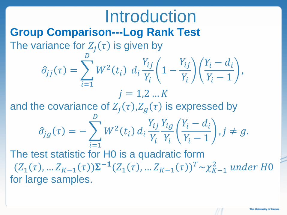
Introduction Group Comparison---Log Rank Test The variance for 𝑍𝑍𝑗𝑗 𝜏𝜏 is given by
𝜎𝜎�𝑗𝑗𝑗𝑗 𝜏𝜏 = �𝑊𝑊2 𝑡𝑡𝑖𝑖
𝐷𝐷
𝑖𝑖=1
𝑑𝑑𝑖𝑖𝑌𝑌𝑖𝑖𝑗𝑗𝑌𝑌𝑖𝑖
1 −𝑌𝑌𝑖𝑖𝑗𝑗𝑌𝑌𝑖𝑖
𝑌𝑌𝑖𝑖 − 𝑑𝑑𝑖𝑖𝑌𝑌𝑖𝑖 − 1
,
𝑗𝑗 = 1,2 …𝐾𝐾 and the covariance of 𝑍𝑍𝑗𝑗 𝜏𝜏 ,𝑍𝑍𝑔𝑔 𝜏𝜏 is expressed by
𝜎𝜎�𝑗𝑗𝑔𝑔 𝜏𝜏 = −�𝑊𝑊2 𝑡𝑡𝑖𝑖
𝐷𝐷
𝑖𝑖=1
𝑑𝑑𝑖𝑖𝑌𝑌𝑖𝑖𝑗𝑗𝑌𝑌𝑖𝑖𝑌𝑌𝑖𝑖𝑔𝑔𝑌𝑌𝑖𝑖
𝑌𝑌𝑖𝑖 − 𝑑𝑑𝑖𝑖𝑌𝑌𝑖𝑖 − 1
, 𝑗𝑗 ≠ 𝑔𝑔.
The test statistic for H0 is a quadratic form (𝑍𝑍1 𝜏𝜏 , …𝑍𝑍𝐾𝐾−1 𝜏𝜏 )𝚺𝚺−𝟏𝟏(𝑍𝑍1 𝜏𝜏 , …𝑍𝑍𝐾𝐾−1 𝜏𝜏 )𝑇𝑇~𝜒𝜒𝐾𝐾−12 𝑢𝑢𝑛𝑛𝑑𝑑𝑒𝑒𝑑𝑑 𝐻𝐻𝐻
for large samples.
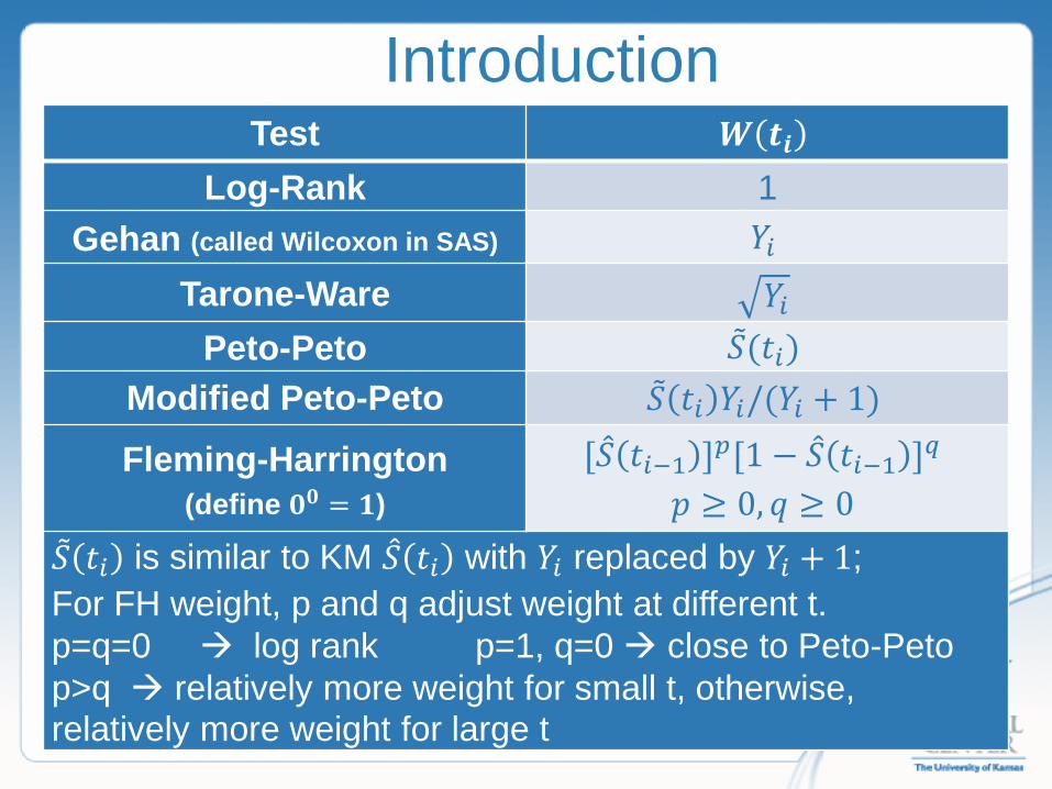
Introduction Test 𝑾𝑾 𝒕𝒕𝒊𝒊
Log-Rank 1 Gehan (called Wilcoxon in SAS) 𝑌𝑌𝑖𝑖
Tarone-Ware 𝑌𝑌𝑖𝑖 Peto-Peto �̃�𝑆(𝑡𝑡𝑖𝑖)
Modified Peto-Peto �̃�𝑆 𝑡𝑡𝑖𝑖 𝑌𝑌𝑖𝑖/(𝑌𝑌𝑖𝑖 + 1)
Fleming-Harrington (define 𝟎𝟎𝟎𝟎 = 𝟏𝟏)
[�̂�𝑆 𝑡𝑡𝑖𝑖−1 ]𝑝𝑝[1 − �̂�𝑆 𝑡𝑡𝑖𝑖−1 ]𝑞𝑞 𝑝𝑝 ≥ 0, 𝑞𝑞 ≥ 0
�̃�𝑆 𝑡𝑡𝑖𝑖 is similar to KM �̂�𝑆 𝑡𝑡𝑖𝑖 with 𝑌𝑌𝑖𝑖 replaced by 𝑌𝑌𝑖𝑖 + 1; For FH weight, p and q adjust weight at different t. p=q=0 log rank p=1, q=0 close to Peto-Peto p>q relatively more weight for small t, otherwise, relatively more weight for large t
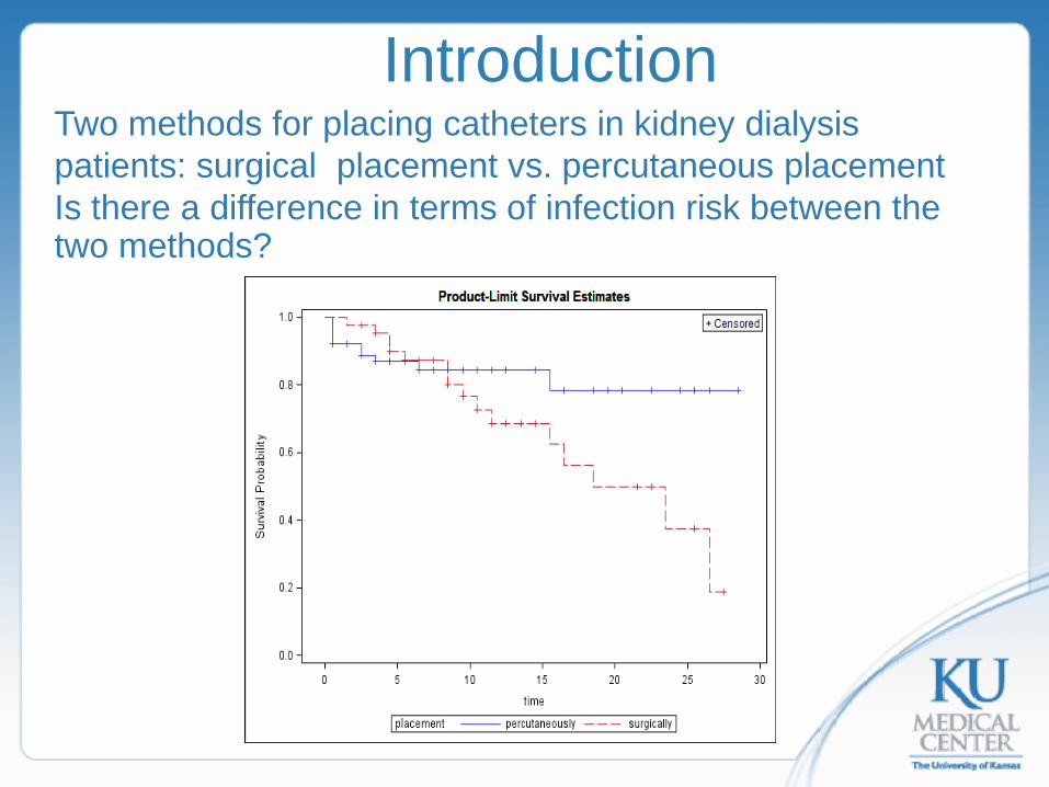
Introduction Two methods for placing catheters in kidney dialysis patients: surgical placement vs. percutaneous placement Is there a difference in terms of infection risk between the two methods?

Introduction Test of Equality over Group
Pr > Test Chi-Square DF Chi-Square Log-Rank 2.5295 1 0.1117 Wilcoxon 0.0021 1 0.9636 Tarone 0.4027 1 0.5257 Peto 1.3992 1 0.2369 Modified Peto 1.2759 1 0.2587 Fleming(0,1) 9.6680 1 0.0019 proc lifetest data=kidney outsurv=a; time time*infect(0); strata /test= all group=placement FLEMING(0, 1); run; *All include FLEMING(1,0) (default). When FLEMING(0, 1) is specified, FLEMING(1,0) will be replaced;

Introduction With different weight functions, different conclusions can be made. In reality, which weight to use should be pre-specified based on clinical considerations. For example, sometimes it may be more relevant to consider the difference between two treatments immediately after baseline. Note: these tests average differences across time that they are not appropriate for survival functions crossing each other.
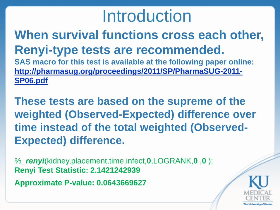
Introduction When survival functions cross each other, Renyi-type tests are recommended. SAS macro for this test is available at the following paper online: http://pharmasug.org/proceedings/2011/SP/PharmaSUG-2011-SP06.pdf These tests are based on the supreme of the weighted (Observed-Expected) difference over time instead of the total weighted (Observed-Expected) difference. %_renyi(kidney,placement,time,infect,0,LOGRANK,0 ,0 ); Renyi Test Statistic: 2.1421242939 Approximate P-value: 0.0643669627

Introduction Test for trend Assume there are K samples Null hypothesis: For 𝑡𝑡 ≤ 𝜏𝜏,
𝐻𝐻0: ℎ1 𝑡𝑡 = ℎ2 𝑡𝑡 = ⋯ = ℎ𝐾𝐾 𝑡𝑡 Alternative hypothesis: For 𝑡𝑡 ≤ 𝜏𝜏
𝐻𝐻𝐴𝐴:ℎ1 𝑡𝑡 ≤ ℎ2 𝑡𝑡 ≤ ⋯ ≤ ℎ𝐾𝐾 𝑡𝑡 with at least one strict inequality
proc lifetest data=Larynx; time time*death(0); strata /trend group=stage all; run;

Introduction Test for trend--Larynx cancer patients at different stages
Test z-Score Pr > |z| Log-Rank 3.7190 0.0002 Wilcoxon 4.2248 <.0001 Tarone 4.0580 <.0001 Peto 4.1293 <.0001 Modified Peto 4.1363 <.0001
Fleming(1) 4.1201 <.0001
When there is no censoring, the test using Gehan or Peto-Peto weights reduces to the Jonckheere-Terpstra test (trend test for categorical data).
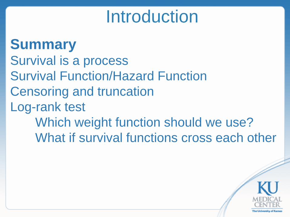
Introduction Summary Survival is a process Survival Function/Hazard Function Censoring and truncation Log-rank test Which weight function should we use? What if survival functions cross each other
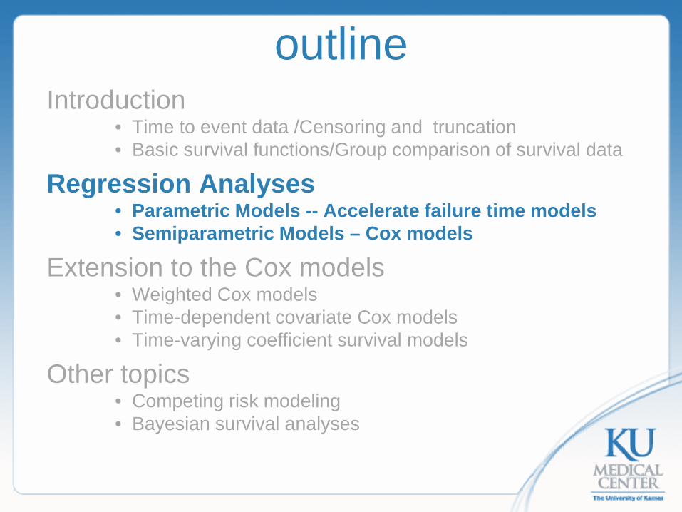
outline Introduction
• Time to event data /Censoring and truncation • Basic survival functions/Group comparison of survival data
Regression Analyses • Parametric Models -- Accelerate failure time models • Semiparametric Models – Cox models
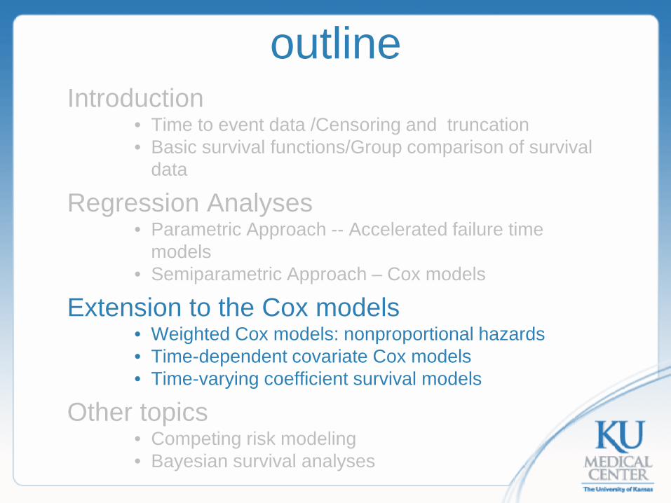
Extension to the Cox models • Weighted Cox models • Time-dependent covariate Cox models • Time-varying coefficient survival models
Other topics • Competing risk modeling • Bayesian survival analyses
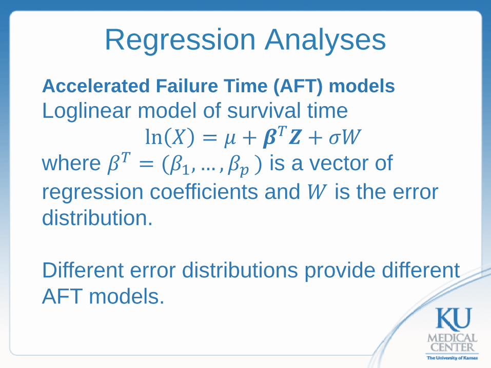
Regression Analyses Accelerated Failure Time (AFT) models Loglinear model of survival time
ln 𝑋𝑋 = 𝜇𝜇 + 𝜷𝜷𝑇𝑇𝒁𝒁 + 𝜎𝜎𝑊𝑊 where 𝛽𝛽𝑇𝑇 = (𝛽𝛽1, … ,𝛽𝛽𝑝𝑝 ) is a vector of regression coefficients and 𝑊𝑊 is the error distribution. Different error distributions provide different AFT models.
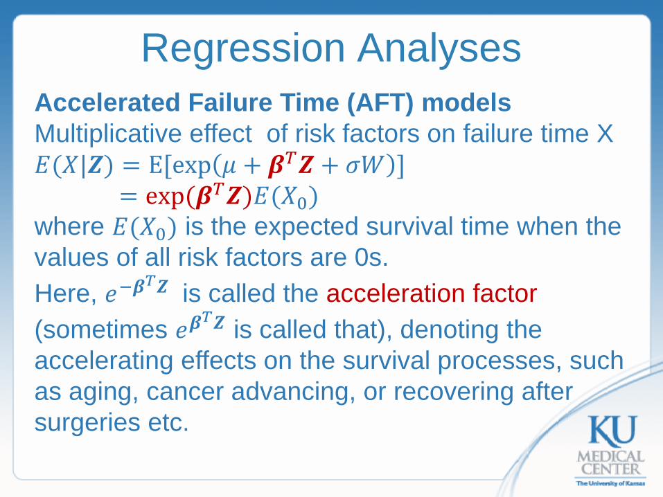
Regression Analyses Accelerated Failure Time (AFT) models Multiplicative effect of risk factors on failure time X 𝐸𝐸(𝑋𝑋|𝒁𝒁) = E[exp 𝜇𝜇 + 𝜷𝜷𝑇𝑇𝒁𝒁 + 𝜎𝜎𝑊𝑊 ] = exp (𝜷𝜷𝑇𝑇𝒁𝒁)𝐸𝐸(𝑋𝑋0) where 𝐸𝐸(𝑋𝑋0) is the expected survival time when the values of all risk factors are 0s. Here, 𝑒𝑒−𝜷𝜷𝑇𝑇𝒁𝒁 is called the acceleration factor (sometimes 𝑒𝑒𝜷𝜷𝑇𝑇𝒁𝒁 is called that), denoting the accelerating effects on the survival processes, such as aging, cancer advancing, or recovering after surgeries etc.
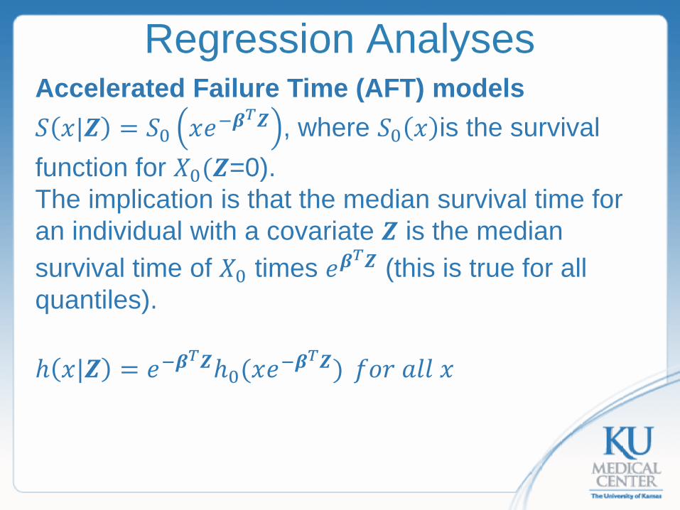
Regression Analyses Accelerated Failure Time (AFT) models 𝑆𝑆 𝑥𝑥|𝒁𝒁 = 𝑆𝑆0 𝑥𝑥𝑒𝑒−𝜷𝜷𝑇𝑇𝒁𝒁 , where 𝑆𝑆0 𝑥𝑥 is the survival function for 𝑋𝑋0(𝒁𝒁=0). The implication is that the median survival time for an individual with a covariate 𝒁𝒁 is the median survival time of 𝑋𝑋0 times 𝑒𝑒𝜷𝜷𝑇𝑇𝒁𝒁 (this is true for all quantiles). ℎ 𝑥𝑥|𝒁𝒁 = 𝑒𝑒−𝜷𝜷𝑇𝑇𝒁𝒁ℎ0(𝑥𝑥𝑒𝑒−𝜷𝜷𝑇𝑇𝒁𝒁) 𝑓𝑓𝑜𝑜𝑑𝑑 𝑎𝑎𝑙𝑙𝑙𝑙 𝑥𝑥
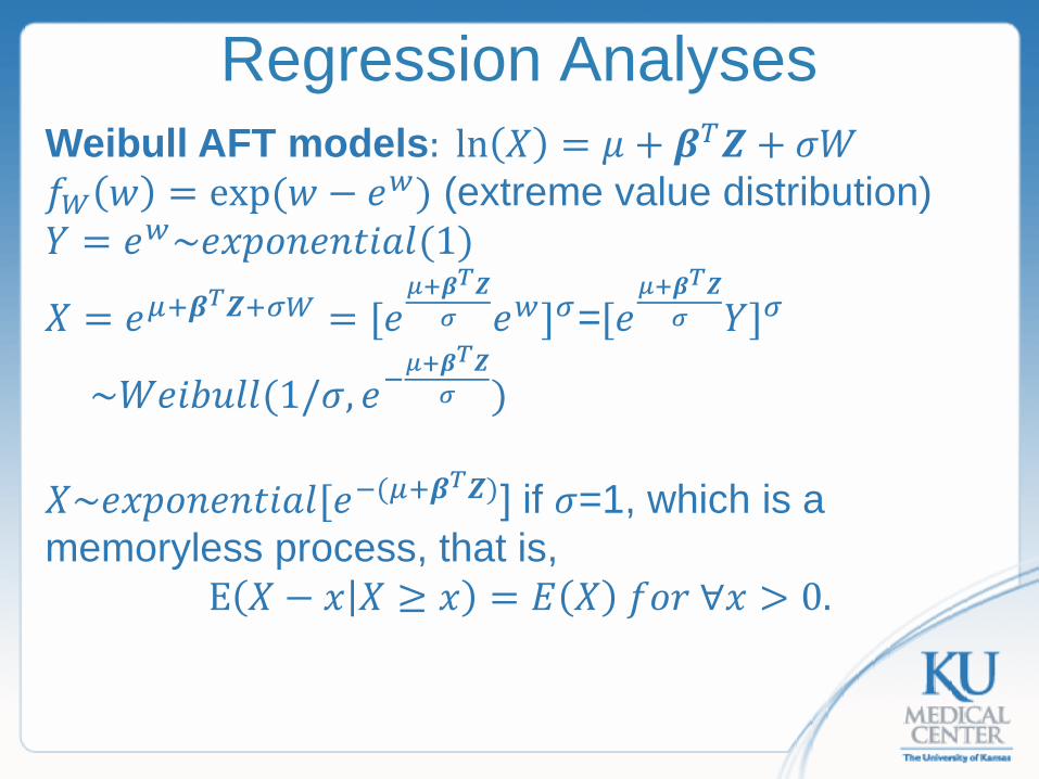
Regression Analyses Weibull AFT models: ln 𝑋𝑋 = 𝜇𝜇 + 𝜷𝜷𝑇𝑇𝒁𝒁 + 𝜎𝜎𝑊𝑊 𝑓𝑓𝑊𝑊 𝑤𝑤 = exp(𝑤𝑤 − 𝑒𝑒𝑤𝑤) (extreme value distribution) 𝑌𝑌 = 𝑒𝑒𝑤𝑤~𝑒𝑒𝑥𝑥𝑝𝑝𝑜𝑜𝑛𝑛𝑒𝑒𝑛𝑛𝑡𝑡𝑖𝑖𝑎𝑎𝑙𝑙(1)
𝑋𝑋 = 𝑒𝑒𝜇𝜇+𝜷𝜷𝑇𝑇𝒁𝒁+𝜎𝜎𝑊𝑊 = [𝑒𝑒𝜇𝜇+𝜷𝜷𝑇𝑇𝒁𝒁
𝜎𝜎 𝑒𝑒𝑤𝑤]𝜎𝜎=[𝑒𝑒𝜇𝜇+𝜷𝜷𝑇𝑇𝒁𝒁
𝜎𝜎 𝑌𝑌]𝜎𝜎
~𝑊𝑊𝑒𝑒𝑖𝑖𝑊𝑊𝑢𝑢𝑙𝑙𝑙𝑙(1/𝜎𝜎, 𝑒𝑒−𝜇𝜇+𝜷𝜷𝑇𝑇𝒁𝒁
𝜎𝜎 ) 𝑋𝑋~𝑒𝑒𝑥𝑥𝑝𝑝𝑜𝑜𝑛𝑛𝑒𝑒𝑛𝑛𝑡𝑡𝑖𝑖𝑎𝑎𝑙𝑙[𝑒𝑒−(𝜇𝜇+𝜷𝜷𝑇𝑇𝒁𝒁)] if 𝜎𝜎=1, which is a memoryless process, that is,
E 𝑋𝑋 − 𝑥𝑥 𝑋𝑋 ≥ 𝑥𝑥 = 𝐸𝐸 𝑋𝑋 𝑓𝑓𝑜𝑜𝑑𝑑 ∀𝑥𝑥 > 0.
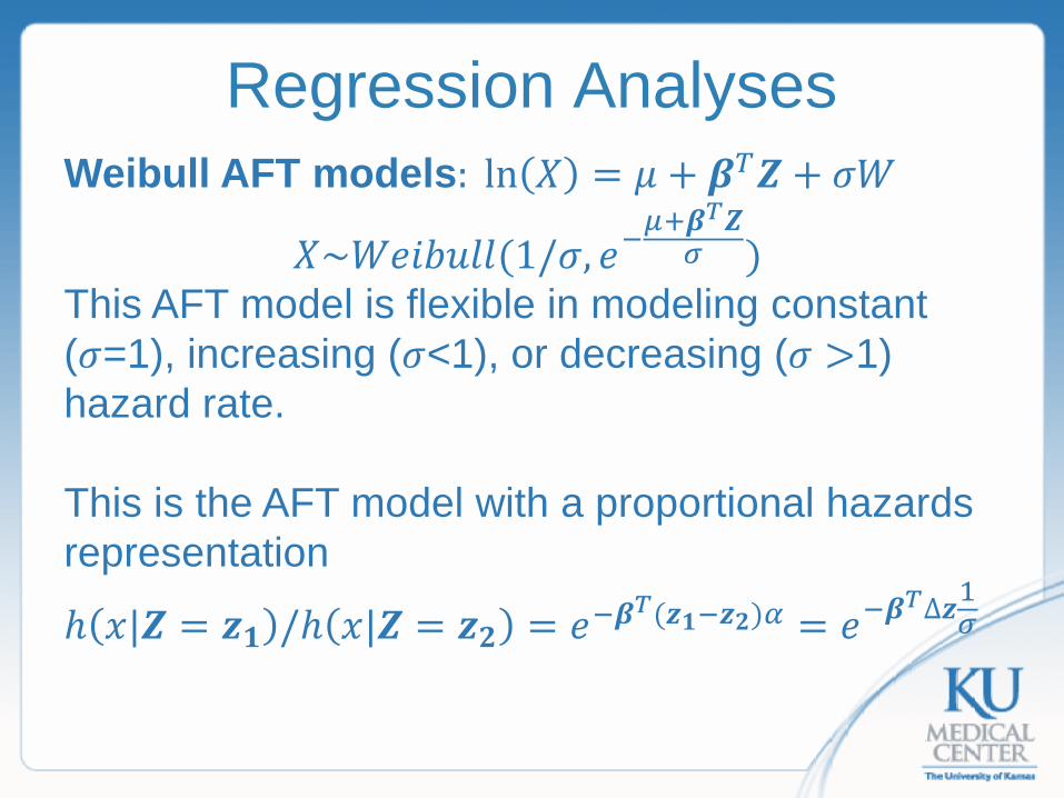
Regression Analyses Weibull AFT models: ln 𝑋𝑋 = 𝜇𝜇 + 𝜷𝜷𝑇𝑇𝒁𝒁 + 𝜎𝜎𝑊𝑊
𝑋𝑋~𝑊𝑊𝑒𝑒𝑖𝑖𝑊𝑊𝑢𝑢𝑙𝑙𝑙𝑙(1/𝜎𝜎, 𝑒𝑒−𝜇𝜇+𝜷𝜷𝑇𝑇𝒁𝒁
𝜎𝜎 ) This AFT model is flexible in modeling constant (𝜎𝜎=1), increasing (𝜎𝜎<1), or decreasing (𝜎𝜎 >1) hazard rate. This is the AFT model with a proportional hazards representation
ℎ 𝑥𝑥|𝒁𝒁 = 𝒛𝒛𝟏𝟏 /ℎ 𝑥𝑥|𝒁𝒁 = 𝒛𝒛𝟐𝟐 = 𝑒𝑒−𝜷𝜷𝑇𝑇(𝒛𝒛𝟏𝟏−𝒛𝒛𝟐𝟐)𝛼𝛼 = 𝑒𝑒−𝜷𝜷𝑇𝑇∆𝒛𝒛1𝜎𝜎
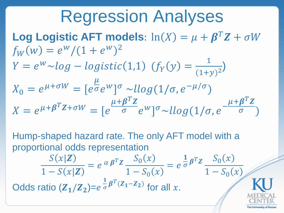
Regression Analyses Log Logistic AFT models: ln 𝑋𝑋 = 𝜇𝜇 + 𝜷𝜷𝑇𝑇𝒁𝒁 + 𝜎𝜎𝑊𝑊 𝑓𝑓𝑊𝑊 𝑤𝑤 = 𝑒𝑒𝑤𝑤/(1 + 𝑒𝑒𝑤𝑤)2 𝑌𝑌 = 𝑒𝑒𝑤𝑤~𝑙𝑙𝑜𝑜𝑔𝑔 − 𝑙𝑙𝑜𝑜𝑔𝑔𝑖𝑖𝑙𝑙𝑡𝑡𝑖𝑖𝑐𝑐 1,1 (𝑓𝑓𝑌𝑌 𝑦𝑦 = 1
(1+𝑦𝑦)2)
𝑋𝑋0 = 𝑒𝑒𝜇𝜇+𝜎𝜎𝑊𝑊 = [𝑒𝑒𝜇𝜇𝜎𝜎𝑒𝑒𝑤𝑤]𝜎𝜎 ~𝑙𝑙𝑙𝑙𝑜𝑜𝑔𝑔(1/𝜎𝜎, 𝑒𝑒−𝜇𝜇/𝜎𝜎)
𝑋𝑋 = 𝑒𝑒𝜇𝜇+𝜷𝜷𝑇𝑇𝒁𝒁+𝜎𝜎𝑊𝑊 = [𝑒𝑒𝜇𝜇+𝜷𝜷𝑇𝑇𝒁𝒁
𝜎𝜎 𝑒𝑒𝑤𝑤]𝜎𝜎~𝑙𝑙𝑙𝑙𝑜𝑜𝑔𝑔(1/𝜎𝜎, 𝑒𝑒−𝜇𝜇+𝜷𝜷𝑇𝑇𝒁𝒁
𝜎𝜎 ) Hump-shaped hazard rate. The only AFT model with a proportional odds representation
𝑆𝑆 𝑥𝑥|𝒁𝒁1 − 𝑆𝑆 𝑥𝑥|𝒁𝒁
= 𝑒𝑒 𝛼𝛼 𝜷𝜷𝑇𝑇𝒁𝒁 𝑆𝑆0 𝑥𝑥1 − 𝑆𝑆0 𝑥𝑥
= 𝑒𝑒 𝟏𝟏𝜎𝜎 𝜷𝜷𝑇𝑇𝒁𝒁 𝑆𝑆0 𝑥𝑥1 − 𝑆𝑆0 𝑥𝑥
Odds ratio (𝒁𝒁𝟏𝟏/𝒁𝒁𝟐𝟐)=𝑒𝑒 𝟏𝟏𝜎𝜎 𝜷𝜷𝑇𝑇(𝒁𝒁𝟏𝟏−𝒁𝒁𝟐𝟐) for all 𝑥𝑥.
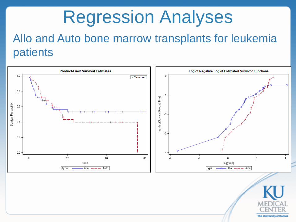
Regression Analyses Allo and Auto bone marrow transplants for leukemia patients
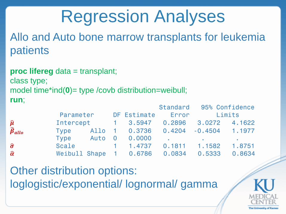
Regression Analyses Allo and Auto bone marrow transplants for leukemia patients proc lifereg data = transplant; class type; model time*ind(0)= type /covb distribution=weibull; run; Standard 95% Confidence Parameter DF Estimate Error Limits 𝝁𝝁� Intercept 1 3.5947 0.2896 3.0272 4.1622 𝜷𝜷�𝒂𝒂𝒂𝒂𝒂𝒂𝒂𝒂 Type Allo 1 0.3736 0.4204 -0.4504 1.1977 Type Auto 0 0.0000 . . . 𝝈𝝈� Scale 1 1.4737 0.1811 1.1582 1.8751 𝜶𝜶� Weibull Shape 1 0.6786 0.0834 0.5333 0.8634
Other distribution options: loglogistic/exponential/ lognormal/ gamma
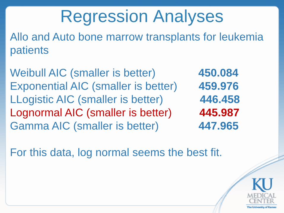
Regression Analyses Allo and Auto bone marrow transplants for leukemia patients Weibull AIC (smaller is better) 450.084 Exponential AIC (smaller is better) 459.976 LLogistic AIC (smaller is better) 446.458 Lognormal AIC (smaller is better) 445.987 Gamma AIC (smaller is better) 447.965 For this data, log normal seems the best fit.
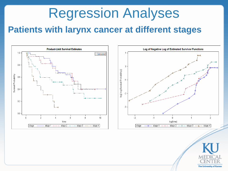
Regression Analyses Patients with larynx cancer at different stages
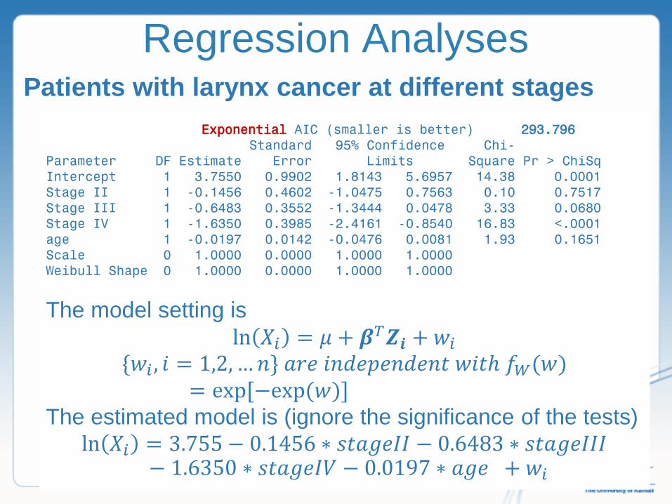
Regression Analyses Patients with larynx cancer at different stages
Exponential AIC (smaller is better) 293.796 Standard 95% Confidence Chi- Parameter DF Estimate Error Limits Square Pr > ChiSq Intercept 1 3.7550 0.9902 1.8143 5.6957 14.38 0.0001 Stage II 1 -0.1456 0.4602 -1.0475 0.7563 0.10 0.7517 Stage III 1 -0.6483 0.3552 -1.3444 0.0478 3.33 0.0680 Stage IV 1 -1.6350 0.3985 -2.4161 -0.8540 16.83 <.0001 age 1 -0.0197 0.0142 -0.0476 0.0081 1.93 0.1651 Scale 0 1.0000 0.0000 1.0000 1.0000 Weibull Shape 0 1.0000 0.0000 1.0000 1.0000
The model setting is ln 𝑋𝑋𝑖𝑖 = 𝜇𝜇 + 𝜷𝜷𝑇𝑇𝒁𝒁𝒊𝒊 + 𝑤𝑤𝑖𝑖
{𝑤𝑤𝑖𝑖 , 𝑖𝑖 = 1,2, …𝑛𝑛} 𝑎𝑎𝑑𝑑𝑒𝑒 𝑖𝑖𝑛𝑛𝑑𝑑𝑒𝑒𝑝𝑝𝑒𝑒𝑛𝑛𝑑𝑑𝑒𝑒𝑛𝑛𝑡𝑡 𝑤𝑤𝑖𝑖𝑡𝑡ℎ 𝑓𝑓𝑊𝑊(𝑤𝑤)= exp[−exp(𝑤𝑤)]
The estimated model is (ignore the significance of the tests) ln 𝑋𝑋𝑖𝑖 = 3.755 − 0.1456 ∗ 𝑙𝑙𝑡𝑡𝑎𝑎𝑔𝑔𝑒𝑒𝐼𝐼𝐼𝐼 − 0.6483 ∗ 𝑙𝑙𝑡𝑡𝑎𝑎𝑔𝑔𝑒𝑒𝐼𝐼𝐼𝐼𝐼𝐼
− 1.6350 ∗ 𝑙𝑙𝑡𝑡𝑎𝑎𝑔𝑔𝑒𝑒𝐼𝐼𝑉𝑉 − 0.0197 ∗ 𝑎𝑎𝑔𝑔𝑒𝑒 + 𝑤𝑤𝑖𝑖
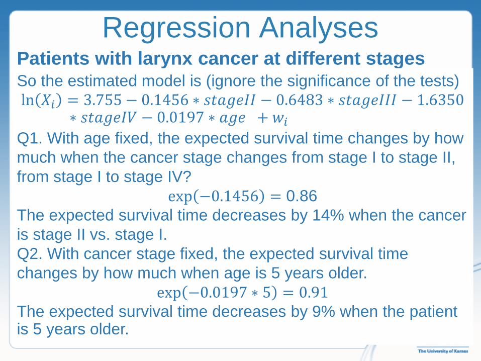
Regression Analyses Patients with larynx cancer at different stages So the estimated model is (ignore the significance of the tests) ln 𝑋𝑋𝑖𝑖 = 3.755 − 0.1456 ∗ 𝑙𝑙𝑡𝑡𝑎𝑎𝑔𝑔𝑒𝑒𝐼𝐼𝐼𝐼 − 0.6483 ∗ 𝑙𝑙𝑡𝑡𝑎𝑎𝑔𝑔𝑒𝑒𝐼𝐼𝐼𝐼𝐼𝐼 − 1.6350
∗ 𝑙𝑙𝑡𝑡𝑎𝑎𝑔𝑔𝑒𝑒𝐼𝐼𝑉𝑉 − 0.0197 ∗ 𝑎𝑎𝑔𝑔𝑒𝑒 + 𝑤𝑤𝑖𝑖 Q1. With age fixed, the expected survival time changes by how much when the cancer stage changes from stage I to stage II, from stage I to stage IV?
exp −0.1456 = 0.86 The expected survival time decreases by 14% when the cancer is stage II vs. stage I. Q2. With cancer stage fixed, the expected survival time changes by how much when age is 5 years older.
exp −0.0197 ∗ 5 = 0.91 The expected survival time decreases by 9% when the patient is 5 years older.

Regression Analyses Patients with larynx cancer at different stages So the estimated model is (ignore the significance of the tests) ln 𝑋𝑋𝑖𝑖 = 3.755 − 0.1456 ∗ 𝑙𝑙𝑡𝑡𝑎𝑎𝑔𝑔𝑒𝑒𝐼𝐼𝐼𝐼 − 0.6483 ∗ 𝑙𝑙𝑡𝑡𝑎𝑎𝑔𝑔𝑒𝑒𝐼𝐼𝐼𝐼𝐼𝐼 − 1.6350
∗ 𝑙𝑙𝑡𝑡𝑎𝑎𝑔𝑔𝑒𝑒𝐼𝐼𝑉𝑉 − 0.0197 ∗ 𝑎𝑎𝑔𝑔𝑒𝑒 + 𝑤𝑤𝑖𝑖 Q3. What is the median survival time for an individual of age 65 with Larynx cancer of stage I, stage II, stage III, and Stage IV? Y = exp 𝑤𝑤 ~𝑒𝑒𝑥𝑥𝑝𝑝𝑜𝑜𝑛𝑛𝑒𝑒𝑛𝑛𝑡𝑡𝑖𝑖𝑎𝑎𝑙𝑙 1 S y = 𝑒𝑒𝑥𝑥𝑝𝑝 −𝑦𝑦 = 0.5 ⇒ 𝑀𝑀𝑦𝑦 = ln(2) 𝑀𝑀(𝑠𝑠𝑡𝑡𝑔𝑔𝐼𝐼,𝑎𝑎𝑔𝑔𝑎𝑎=65) = exp 3.755 − 0.0197 ∗ 65 ∗ 𝑀𝑀𝑦𝑦=8.2 yrs 𝑀𝑀(𝑠𝑠𝑡𝑡𝑔𝑔𝐼𝐼𝐼𝐼,𝑎𝑎𝑔𝑔𝑎𝑎=65) = exp 3.755 − 0.1456 − 0.0197 ∗ 65 ∗ 𝑀𝑀𝑦𝑦=7.1 yrs 𝑀𝑀(𝑠𝑠𝑡𝑡𝑔𝑔𝐼𝐼𝐼𝐼𝐼𝐼,𝑎𝑎𝑔𝑔𝑎𝑎=65) = exp 3.755 − 0.6483 − 0.0197 ∗ 65 ∗ 𝑀𝑀𝑦𝑦=4.3 yrs 𝑀𝑀(𝑠𝑠𝑡𝑡𝑔𝑔𝑠𝑠,𝑎𝑎𝑔𝑔𝑎𝑎=65) = exp 3.755 − 1.6350 − 0.0197 ∗ 65 ∗ 𝑀𝑀𝑦𝑦 =1.6 yrs

Regression Analyses Summary---AFT models Parametric models with options for different hazard function forms (constant, increasing, decreasing, hump-shaped) Multiplicative effects of factors on survival times This type of models are not used as commonly as general linear models for continuous variables in reality. Why? A more flexible model that is easy to implement: The Cox model
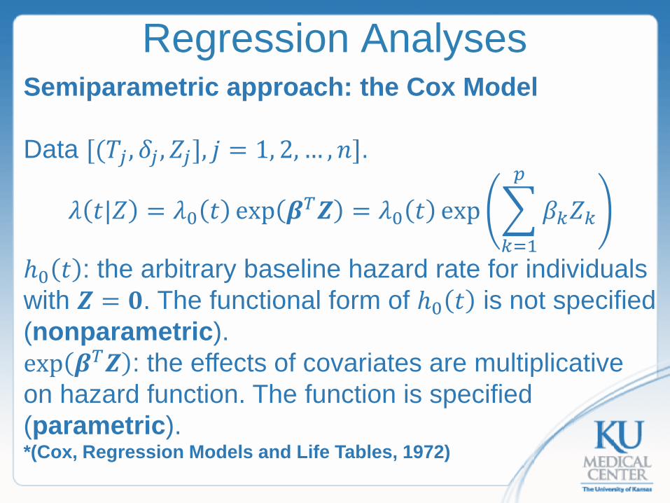
Regression Analyses Semiparametric approach: the Cox Model Data [(𝑇𝑇𝑗𝑗 , 𝛿𝛿𝑗𝑗 ,𝑍𝑍𝑗𝑗], 𝑗𝑗 = 1, 2, … ,𝑛𝑛].
𝜆𝜆 𝑡𝑡|𝑍𝑍 = 𝜆𝜆0 𝑡𝑡 exp 𝜷𝜷𝑇𝑇𝒁𝒁 = 𝜆𝜆0 𝑡𝑡 exp �𝛽𝛽𝑘𝑘𝑍𝑍𝑘𝑘
𝑝𝑝
𝑘𝑘=1
ℎ0 𝑡𝑡 : the arbitrary baseline hazard rate for individuals with 𝒁𝒁 = 𝟎𝟎. The functional form of ℎ0 𝑡𝑡 is not specified (nonparametric). exp 𝜷𝜷𝑇𝑇𝒁𝒁 : the effects of covariates are multiplicative on hazard function. The function is specified (parametric). *(Cox, Regression Models and Life Tables, 1972)
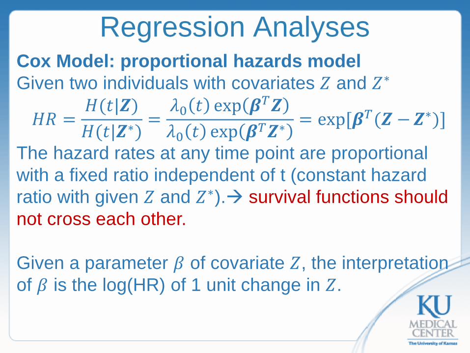
Regression Analyses Cox Model: proportional hazards model Given two individuals with covariates 𝑍𝑍 and 𝑍𝑍∗
𝐻𝐻𝐻𝐻 =𝐻𝐻(𝑡𝑡|𝒁𝒁)𝐻𝐻(𝑡𝑡|𝒁𝒁∗)
=𝜆𝜆0 𝑡𝑡 exp 𝜷𝜷𝑇𝑇𝒁𝒁𝜆𝜆0 𝑡𝑡 exp 𝜷𝜷𝑇𝑇𝒁𝒁∗
= exp[𝜷𝜷𝑇𝑇(𝒁𝒁 −𝒁𝒁∗)]
The hazard rates at any time point are proportional with a fixed ratio independent of t (constant hazard ratio with given 𝑍𝑍 and 𝑍𝑍∗). survival functions should not cross each other. Given a parameter 𝛽𝛽 of covariate 𝑍𝑍, the interpretation of 𝛽𝛽 is the log(HR) of 1 unit change in 𝑍𝑍.
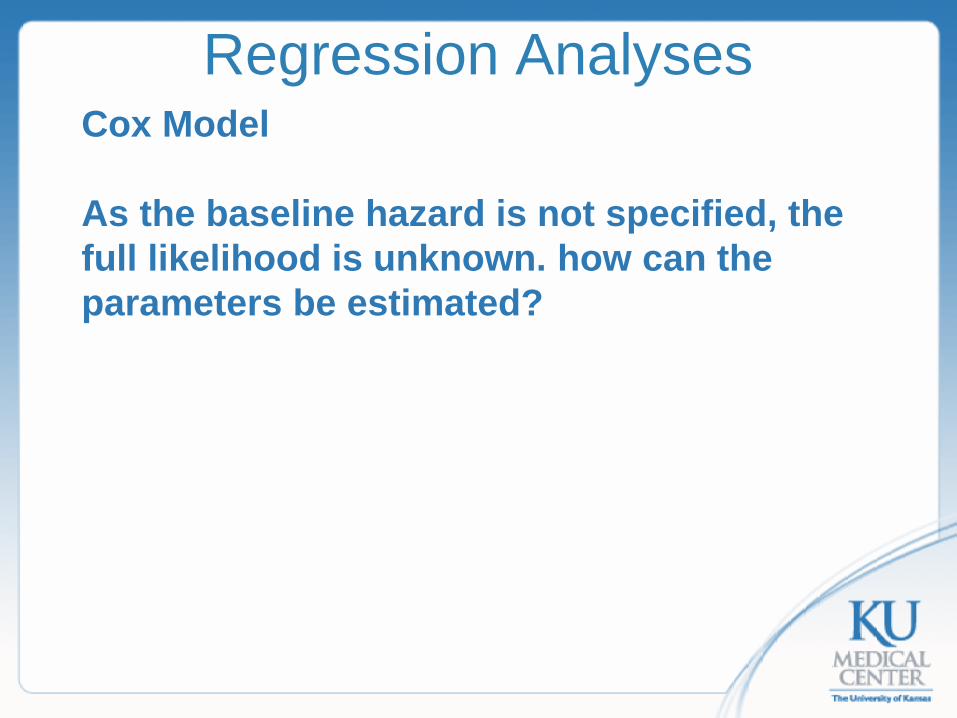
Regression Analyses Cox Model As the baseline hazard is not specified, the full likelihood is unknown. how can the parameters be estimated?
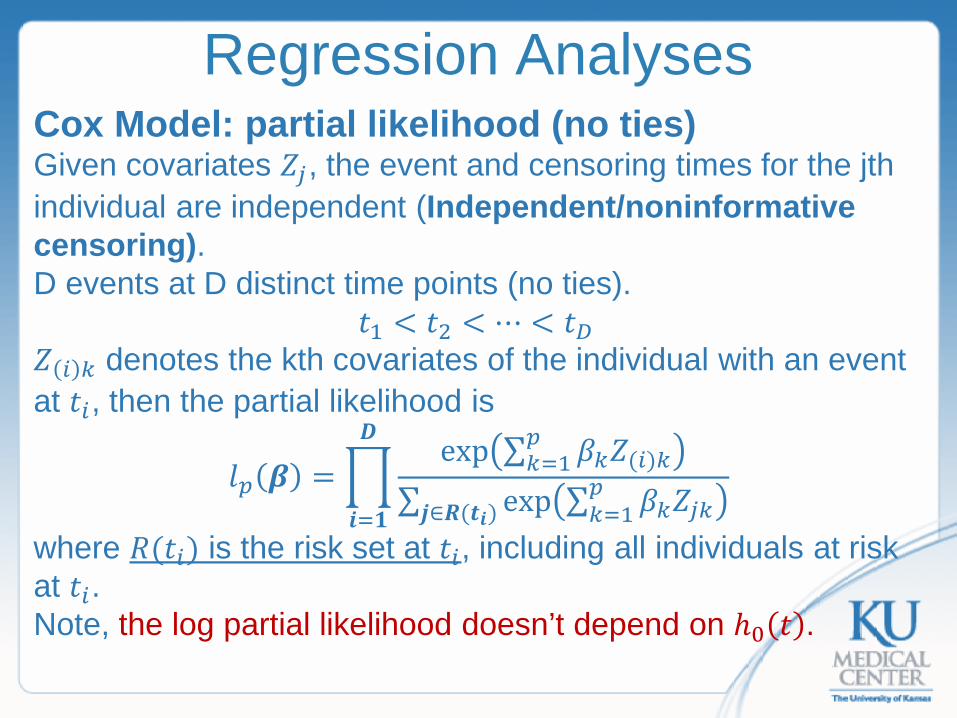
Regression Analyses Cox Model: partial likelihood (no ties) Given covariates 𝑍𝑍𝑗𝑗, the event and censoring times for the jth individual are independent (Independent/noninformative censoring). D events at D distinct time points (no ties).
𝑡𝑡1 < 𝑡𝑡2 < ⋯ < 𝑡𝑡𝐷𝐷 𝑍𝑍 𝑖𝑖 𝑘𝑘 denotes the kth covariates of the individual with an event at 𝑡𝑡𝑖𝑖, then the partial likelihood is
𝑙𝑙𝑝𝑝 𝜷𝜷 = �exp ∑ 𝛽𝛽𝑘𝑘𝑍𝑍(𝑖𝑖)𝑘𝑘
𝑝𝑝𝑘𝑘=1
∑ exp ∑ 𝛽𝛽𝑘𝑘𝑍𝑍𝑗𝑗𝑘𝑘𝑝𝑝𝑘𝑘=1𝒋𝒋∈𝑹𝑹(𝒕𝒕𝒊𝒊)
𝑫𝑫
𝒊𝒊=𝟏𝟏
where 𝐻𝐻(𝑡𝑡𝑖𝑖) is the risk set at 𝑡𝑡𝑖𝑖, including all individuals at risk at 𝑡𝑡𝑖𝑖. Note, the log partial likelihood doesn’t depend on ℎ0 𝑡𝑡 .
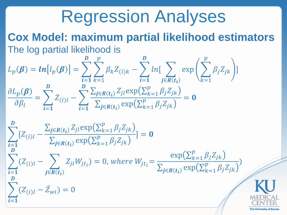
Regression Analyses Cox Model: maximum partial likelihood estimators The log partial likelihood is
𝐿𝐿𝑝𝑝 𝜷𝜷 = 𝒂𝒂𝒍𝒍 𝑙𝑙𝑝𝑝 𝜷𝜷 = ��𝛽𝛽𝑘𝑘𝑍𝑍(𝑖𝑖)𝑘𝑘
𝑝𝑝
𝑘𝑘=1
𝑫𝑫
𝒊𝒊=𝟏𝟏
−�𝑙𝑙𝑛𝑛[ � exp �𝛽𝛽𝑗𝑗𝑍𝑍𝑗𝑗𝑘𝑘
𝑝𝑝
𝑘𝑘=1𝒋𝒋∈𝑹𝑹 𝒕𝒕𝒊𝒊
]𝑫𝑫
𝒊𝒊=𝟏𝟏
𝜕𝜕𝐿𝐿𝑝𝑝 𝜷𝜷𝜕𝜕𝛽𝛽𝑙𝑙
= �𝑍𝑍(𝑖𝑖)𝑙𝑙
𝑫𝑫
𝒊𝒊=𝟏𝟏
−�∑ 𝑍𝑍𝑗𝑗𝑙𝑙exp ∑ 𝛽𝛽𝑗𝑗𝑍𝑍𝑗𝑗𝑘𝑘
𝑝𝑝𝑘𝑘=1𝒋𝒋∈𝑹𝑹 𝒕𝒕𝒊𝒊
∑ exp ∑ 𝛽𝛽𝑗𝑗𝑍𝑍𝑗𝑗𝑘𝑘𝑝𝑝𝑘𝑘=1𝒋𝒋∈𝑹𝑹 𝒕𝒕𝒊𝒊
= 𝟎𝟎𝑫𝑫
𝒊𝒊=𝟏𝟏
�[𝑍𝑍(𝑖𝑖)𝑙𝑙
𝑫𝑫
𝒊𝒊=𝟏𝟏
−∑ 𝑍𝑍𝑗𝑗𝑙𝑙exp ∑ 𝛽𝛽𝑗𝑗𝑍𝑍𝑗𝑗𝑘𝑘
𝑝𝑝𝑘𝑘=1𝒋𝒋∈𝑹𝑹 𝒕𝒕𝒊𝒊
∑ exp ∑ 𝛽𝛽𝑗𝑗𝑍𝑍𝑗𝑗𝑘𝑘𝑝𝑝𝑘𝑘=1𝒋𝒋∈𝑹𝑹 𝒕𝒕𝒊𝒊
] = 𝟎𝟎
�(𝑍𝑍(𝑖𝑖)𝑙𝑙
𝑫𝑫
𝒊𝒊=𝟏𝟏
− � 𝑍𝑍𝑗𝑗𝑙𝑙𝑊𝑊𝑗𝑗𝑡𝑡𝑖𝑖𝒋𝒋∈𝑹𝑹 𝒕𝒕𝒊𝒊
) = 0, 𝑤𝑤ℎ𝑒𝑒𝑑𝑑𝑒𝑒 𝑊𝑊𝑗𝑗𝑡𝑡𝑖𝑖 =exp ∑ 𝛽𝛽𝑗𝑗𝑍𝑍𝑗𝑗𝑘𝑘
𝑝𝑝𝑘𝑘=1
∑ exp ∑ 𝛽𝛽𝑗𝑗𝑍𝑍𝑗𝑗𝑘𝑘𝑝𝑝𝑘𝑘=1𝒋𝒋∈𝑹𝑹 𝒕𝒕𝒊𝒊
)
�(𝑍𝑍(𝑖𝑖)𝑙𝑙
𝑫𝑫
𝒊𝒊=𝟏𝟏
− �̅�𝑍𝑤𝑤𝑖𝑖) = 0
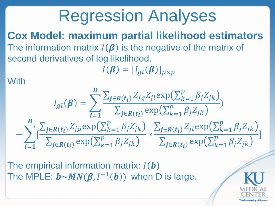
Regression Analyses Cox Model: maximum partial likelihood estimators The information matrix 𝐼𝐼 𝜷𝜷 is the negative of the matrix of second derivatives of log likelihood.
𝐼𝐼 𝜷𝜷 = [𝐼𝐼𝑔𝑔𝑙𝑙 𝜷𝜷 ]𝑝𝑝×𝑝𝑝 With
𝐼𝐼𝑔𝑔𝑙𝑙 𝜷𝜷 = �∑ 𝑍𝑍𝑗𝑗𝑔𝑔𝑍𝑍𝑗𝑗𝑙𝑙exp ∑ 𝛽𝛽𝑗𝑗𝑍𝑍𝑗𝑗𝑘𝑘
𝑝𝑝𝑘𝑘=1𝒋𝒋∈𝑹𝑹 𝒕𝒕𝒊𝒊
∑ exp ∑ 𝛽𝛽𝑗𝑗𝑍𝑍𝑗𝑗𝑘𝑘𝑝𝑝𝑘𝑘=1𝒋𝒋∈𝑹𝑹 𝒕𝒕𝒊𝒊
𝑫𝑫
𝒊𝒊=𝟏𝟏
)
−�[∑ 𝑍𝑍𝑗𝑗𝑔𝑔exp ∑ 𝛽𝛽𝑗𝑗𝑍𝑍𝑗𝑗𝑘𝑘
𝑝𝑝𝑘𝑘=1𝒋𝒋∈𝑹𝑹 𝒕𝒕𝒊𝒊
∑ exp ∑ 𝛽𝛽𝑗𝑗𝑍𝑍𝑗𝑗𝑘𝑘𝑝𝑝𝑘𝑘=1𝒋𝒋∈𝑹𝑹 𝒕𝒕𝒊𝒊
∗𝑫𝑫
𝒊𝒊=𝟏𝟏
∑ 𝑍𝑍𝑗𝑗𝑙𝑙exp ∑ 𝛽𝛽𝑗𝑗𝑍𝑍𝑗𝑗𝑘𝑘𝑝𝑝𝑘𝑘=1𝒋𝒋∈𝑹𝑹 𝒕𝒕𝒊𝒊
∑ exp ∑ 𝛽𝛽𝑗𝑗𝑍𝑍𝑗𝑗𝑘𝑘𝑝𝑝𝑘𝑘=1𝒋𝒋∈𝑹𝑹 𝒕𝒕𝒊𝒊
]
The empirical information matrix: 𝐼𝐼 𝒃𝒃 The MPLE: 𝒃𝒃~𝑴𝑴𝑴𝑴(𝜷𝜷, 𝐼𝐼−1 𝒃𝒃 ) when D is large.
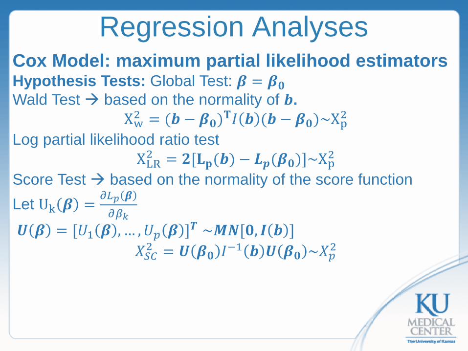
Regression Analyses Cox Model: maximum partial likelihood estimators Hypothesis Tests: Global Test: 𝜷𝜷 = 𝜷𝜷𝟎𝟎 Wald Test based on the normality of 𝒃𝒃.
Χw2 = (𝒃𝒃 − 𝜷𝜷𝟎𝟎)𝐓𝐓𝐼𝐼 𝒃𝒃 (𝒃𝒃 − 𝜷𝜷𝟎𝟎)~Χp2 Log partial likelihood ratio test
ΧLR2 = 𝟐𝟐[𝐋𝐋𝐩𝐩(𝒃𝒃) − 𝑳𝑳𝒑𝒑(𝜷𝜷𝟎𝟎)]~Χp2 Score Test based on the normality of the score function Let Uk 𝜷𝜷 = 𝜕𝜕𝐿𝐿𝑝𝑝 𝜷𝜷
𝜕𝜕𝛽𝛽𝑘𝑘
𝑼𝑼 𝜷𝜷 = [𝑈𝑈1 𝜷𝜷 , … ,𝑈𝑈𝑝𝑝 𝜷𝜷 ]𝑻𝑻 ~𝑴𝑴𝑴𝑴[𝟎𝟎, 𝑰𝑰 𝒃𝒃 ] 𝛸𝛸𝑆𝑆𝑆𝑆2 = 𝑼𝑼 𝜷𝜷𝟎𝟎 𝐼𝐼−1 𝒃𝒃 𝑼𝑼 𝜷𝜷𝟎𝟎 ~𝛸𝛸𝑝𝑝2
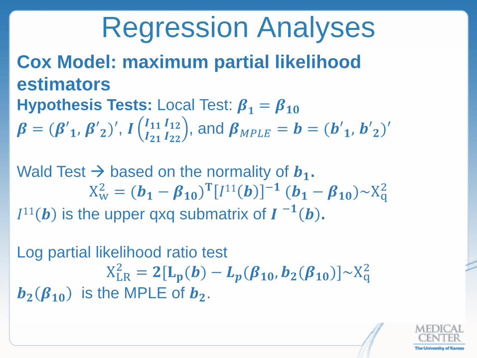
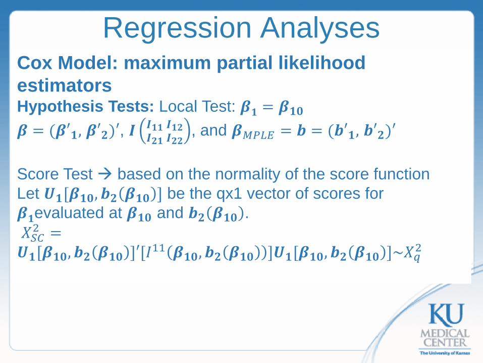
Regression Analyses Cox Model: maximum partial likelihood estimators Hypothesis Tests: Local Test: 𝜷𝜷𝟏𝟏 = 𝜷𝜷𝟏𝟏𝟎𝟎 𝜷𝜷 = (𝜷𝜷𝜷𝟏𝟏, 𝜷𝜷𝜷𝟐𝟐)𝜷, 𝑰𝑰 𝑰𝑰𝟏𝟏𝟏𝟏
𝑰𝑰𝟐𝟐𝟏𝟏𝑰𝑰𝟏𝟏𝟐𝟐𝑰𝑰𝟐𝟐𝟐𝟐
, and 𝜷𝜷𝑀𝑀𝑃𝑃𝐿𝐿𝑀𝑀 = 𝒃𝒃 = (𝒃𝒃𝜷𝟏𝟏, 𝒃𝒃𝜷𝟐𝟐)𝜷 Wald Test based on the normality of 𝒃𝒃𝟏𝟏.
Χw2 = (𝒃𝒃𝟏𝟏 − 𝜷𝜷𝟏𝟏𝟎𝟎)𝐓𝐓 𝐼𝐼11 𝒃𝒃 −𝟏𝟏 (𝒃𝒃𝟏𝟏 − 𝜷𝜷𝟏𝟏𝟎𝟎)~Χq2 𝐼𝐼11 𝒃𝒃 is the upper qxq submatrix of 𝑰𝑰 −𝟏𝟏 𝒃𝒃 . Log partial likelihood ratio test
ΧLR2 = 𝟐𝟐[𝐋𝐋𝐩𝐩(𝒃𝒃) − 𝑳𝑳𝒑𝒑(𝜷𝜷𝟏𝟏𝟎𝟎,𝒃𝒃𝟐𝟐(𝜷𝜷𝟏𝟏𝟎𝟎)]~Χq2 𝒃𝒃𝟐𝟐 𝜷𝜷𝟏𝟏𝟎𝟎 is the MPLE of 𝒃𝒃𝟐𝟐.
Regression Analyses Cox Model: maximum partial likelihood estimators Hypothesis Tests: Local Test: 𝜷𝜷𝟏𝟏 = 𝜷𝜷𝟏𝟏𝟎𝟎 𝜷𝜷 = (𝜷𝜷𝜷𝟏𝟏, 𝜷𝜷𝜷𝟐𝟐)𝜷, 𝑰𝑰 𝑰𝑰𝟏𝟏𝟏𝟏
𝑰𝑰𝟐𝟐𝟏𝟏𝑰𝑰𝟏𝟏𝟐𝟐𝑰𝑰𝟐𝟐𝟐𝟐
, and 𝜷𝜷𝑀𝑀𝑃𝑃𝐿𝐿𝑀𝑀 = 𝒃𝒃 = (𝒃𝒃𝜷𝟏𝟏, 𝒃𝒃𝜷𝟐𝟐)𝜷 Score Test based on the normality of the score function Let 𝑼𝑼𝟏𝟏[𝜷𝜷𝟏𝟏𝟎𝟎,𝒃𝒃𝟐𝟐 𝜷𝜷𝟏𝟏𝟎𝟎 ] be the qx1 vector of scores for 𝜷𝜷𝟏𝟏evaluated at 𝜷𝜷𝟏𝟏𝟎𝟎 and 𝒃𝒃𝟐𝟐 𝜷𝜷𝟏𝟏𝟎𝟎 . 𝛸𝛸𝑆𝑆𝑆𝑆2 =𝑼𝑼𝟏𝟏[𝜷𝜷𝟏𝟏𝟎𝟎,𝒃𝒃𝟐𝟐 𝜷𝜷𝟏𝟏𝟎𝟎 ]𝜷[𝐼𝐼11 𝜷𝜷𝟏𝟏𝟎𝟎,𝒃𝒃𝟐𝟐 𝜷𝜷𝟏𝟏𝟎𝟎 ]𝑼𝑼𝟏𝟏[𝜷𝜷𝟏𝟏𝟎𝟎,𝒃𝒃𝟐𝟐 𝜷𝜷𝟏𝟏𝟎𝟎 ]~𝛸𝛸𝑞𝑞2

Regression Analyses Cox Model: maximum partial likelihood estimators Assume there is only one binary variable Z 𝜆𝜆 𝑡𝑡|𝑍𝑍 = 0 = 𝜆𝜆0 𝑡𝑡 ; 𝜆𝜆 𝑡𝑡|𝑍𝑍 = 1 = 𝜆𝜆0 𝑡𝑡 exp 𝛽𝛽 Hypothesis Test: Local Test: 𝛽𝛽 = 0
𝑈𝑈 𝛽𝛽 = 0 =𝜕𝜕𝐿𝐿𝑝𝑝 𝛽𝛽𝜕𝜕𝛽𝛽 𝛽𝛽=0
= �𝑍𝑍(𝑖𝑖)
𝑫𝑫
𝒊𝒊=𝟏𝟏
−�∑ 𝑍𝑍𝑗𝑗exp 𝛽𝛽𝑍𝑍𝑗𝑗𝒋𝒋∈𝑹𝑹 𝒕𝒕𝒊𝒊∑ exp 𝛽𝛽𝑍𝑍𝑗𝑗𝒋𝒋∈𝑹𝑹 𝒕𝒕𝒊𝒊
𝑫𝑫
𝒊𝒊=𝟏𝟏
= 𝑑𝑑1 −�𝑌𝑌1𝑖𝑖
𝑌𝑌0𝑖𝑖 + 𝑌𝑌1𝑖𝑖
𝑫𝑫
𝒊𝒊=𝟏𝟏
𝑌𝑌0𝑖𝑖 ,𝑌𝑌1𝑖𝑖 are # of subjects at risk at 𝑡𝑡𝑖𝑖
𝐼𝐼 0 = �𝑌𝑌0𝑖𝑖𝑌𝑌1𝑖𝑖
(𝑌𝑌0𝑖𝑖+𝑌𝑌1𝑖𝑖)2
𝑫𝑫
𝒊𝒊=𝟏𝟏
When there are no ties, the score test is exactly the same as the two sample log rank test.

Regression Analyses Cox Model: partial likelihood (with ties) 𝑡𝑡1 < 𝑡𝑡2 < ⋯ < 𝑡𝑡𝐷𝐷 ; 𝑑𝑑𝑖𝑖: # of events at 𝑡𝑡𝑖𝑖; 𝑹𝑹𝑖𝑖: risk set at 𝑡𝑡𝑖𝑖. 𝐷𝐷𝑖𝑖: the set of all individuals who had events at 𝑡𝑡𝑖𝑖 𝑺𝑺𝑖𝑖 = ∑ 𝒁𝒁𝑗𝑗𝑗𝑗∈𝐷𝐷𝑖𝑖 : the sum of the vectors 𝒁𝒁𝑗𝑗over the event set 𝐷𝐷𝑖𝑖. Method 1: Breslow (1974)
𝑙𝑙𝑝𝑝𝐵𝐵 𝜷𝜷 = �exp 𝜷𝜷𝑇𝑇𝑺𝑺𝒊𝒊
[∑ exp 𝜷𝜷𝑇𝑇𝒁𝒁𝒋𝒋 ]𝒅𝒅𝒊𝒊𝒋𝒋∈𝑹𝑹(𝒕𝒕𝒊𝒊)
𝑫𝑫
𝒊𝒊=𝟏𝟏
= ��exp 𝜷𝜷𝑇𝑇𝒁𝒁𝒌𝒌
[∑ exp 𝜷𝜷𝑇𝑇𝒁𝒁𝒋𝒋 ]𝒅𝒅𝒊𝒊𝒋𝒋∈𝑹𝑹(𝒕𝒕𝒊𝒊)𝒌𝒌∈𝐷𝐷𝑖𝑖
=𝑫𝑫
𝒊𝒊=𝟏𝟏
�� �̂�𝑝𝑖𝑖𝑘𝑘𝒌𝒌∈𝐷𝐷𝑖𝑖
𝑫𝑫
𝒊𝒊=𝟏𝟏
This partial likelihood considers each of the 𝑑𝑑𝑖𝑖 events at 𝑡𝑡𝑖𝑖 as distinct, so the conditional probability is the product of the individual conditional probabilities. This approximation works well when there are few ties.
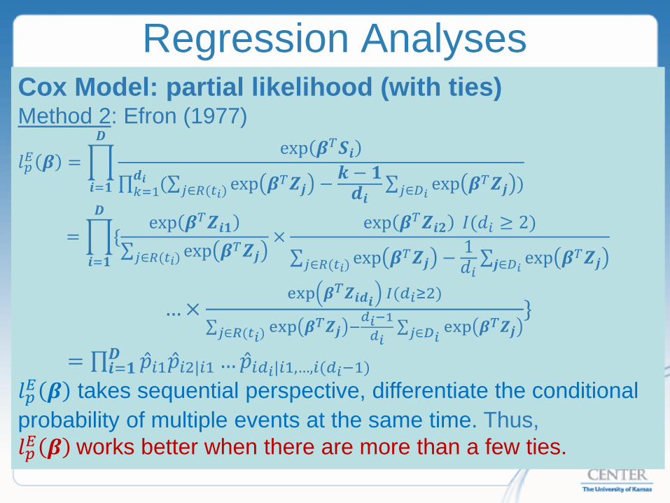
Regression Analyses Cox Model: partial likelihood (with ties) Method 2: Efron (1977)
𝑙𝑙𝑝𝑝𝑀𝑀 𝜷𝜷 = �exp 𝜷𝜷𝑇𝑇𝑺𝑺𝒊𝒊
∏ (∑ exp 𝜷𝜷𝑇𝑇𝒁𝒁𝒋𝒋 − 𝒌𝒌 − 𝟏𝟏𝒅𝒅𝒊𝒊
∑ exp 𝜷𝜷𝑇𝑇𝒁𝒁𝒋𝒋 )𝑗𝑗∈𝐷𝐷𝑖𝑖𝑗𝑗∈𝑅𝑅(𝑡𝑡𝑖𝑖)𝒅𝒅𝒊𝒊𝑘𝑘=1
𝑫𝑫
𝒊𝒊=𝟏𝟏
= �{exp 𝜷𝜷𝑇𝑇𝒁𝒁𝒊𝒊𝟏𝟏
∑ exp 𝜷𝜷𝑇𝑇𝒁𝒁𝒋𝒋𝑗𝑗∈𝑅𝑅(𝑡𝑡𝑖𝑖)×
exp 𝜷𝜷𝑇𝑇𝒁𝒁𝒊𝒊𝟐𝟐 𝐼𝐼(𝑑𝑑𝑖𝑖 ≥ 2)
∑ exp 𝜷𝜷𝑇𝑇𝒁𝒁𝒋𝒋 − 1𝑑𝑑𝑖𝑖∑ exp 𝜷𝜷𝑇𝑇𝒁𝒁𝒋𝒋𝒋𝒋∈𝐷𝐷𝑖𝑖𝑗𝑗∈𝑅𝑅(𝑡𝑡𝑖𝑖)
𝑫𝑫
𝒊𝒊=𝟏𝟏
… ×exp 𝜷𝜷𝑇𝑇𝒁𝒁𝒊𝒊𝒅𝒅𝒊𝒊 𝐼𝐼(𝑑𝑑𝑖𝑖≥2)
∑ exp 𝜷𝜷𝑇𝑇𝒁𝒁𝒋𝒋 −𝑑𝑑𝑖𝑖−1𝑑𝑑𝑖𝑖
∑ exp 𝜷𝜷𝑇𝑇𝒁𝒁𝒋𝒋𝑗𝑗∈𝐷𝐷𝑖𝑖𝑗𝑗∈𝑅𝑅(𝑡𝑡𝑖𝑖)}
= ∏ �̂�𝑝𝑖𝑖1�̂�𝑝𝑖𝑖2|𝑖𝑖1𝑫𝑫𝒊𝒊=𝟏𝟏 … �̂�𝑝𝑖𝑖𝑑𝑑𝑖𝑖|𝑖𝑖1,…,𝑖𝑖(𝑑𝑑𝑖𝑖−1)
𝑙𝑙𝑝𝑝𝑀𝑀 𝜷𝜷 takes sequential perspective, differentiate the conditional probability of multiple events at the same time. Thus, 𝑙𝑙𝑝𝑝𝑀𝑀 𝜷𝜷 works better when there are more than a few ties.
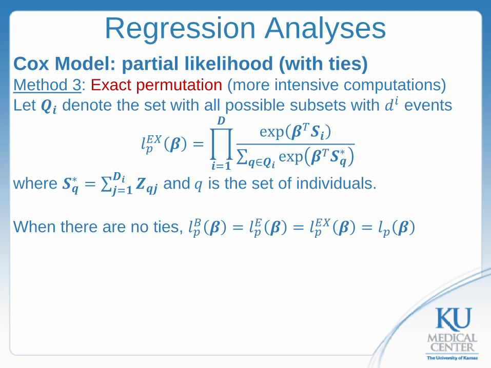
Regression Analyses Cox Model: partial likelihood (with ties) Method 3: Exact permutation (more intensive computations) Let 𝑸𝑸𝒊𝒊 denote the set with all possible subsets with 𝑑𝑑𝑖𝑖 events
𝑙𝑙𝑝𝑝𝑀𝑀𝑋𝑋 𝜷𝜷 = �exp 𝜷𝜷𝑇𝑇𝑺𝑺𝒊𝒊
∑ exp 𝜷𝜷𝑇𝑇𝑺𝑺𝒒𝒒∗𝒒𝒒∈𝑸𝑸𝒊𝒊
𝑫𝑫
𝒊𝒊=𝟏𝟏
where 𝑺𝑺𝒒𝒒∗ = ∑ 𝒁𝒁𝒒𝒒𝒋𝒋𝑫𝑫𝒊𝒊𝒋𝒋=𝟏𝟏 and 𝑞𝑞 is the set of individuals.
When there are no ties, 𝑙𝑙𝑝𝑝𝐵𝐵 𝜷𝜷 = 𝑙𝑙𝑝𝑝𝑀𝑀 𝜷𝜷 = 𝑙𝑙𝑝𝑝𝑀𝑀𝑋𝑋 𝜷𝜷 = 𝑙𝑙𝑝𝑝 𝜷𝜷

Regression Analyses Cox Model: Estimation of the Survival Functions For the proportional hazards model, 𝜆𝜆 𝑡𝑡|𝑍𝑍 = 𝜆𝜆0 𝑡𝑡 exp 𝜷𝜷𝑇𝑇𝒁𝒁 𝐻𝐻 𝑡𝑡|𝑍𝑍 = ∫0
𝑡𝑡𝜆𝜆0 𝜇𝜇 exp 𝜷𝜷𝑇𝑇𝒁𝒁 𝑑𝑑𝜇𝜇= exp 𝜷𝜷𝑇𝑇𝒁𝒁 ∫0
𝑡𝑡𝜆𝜆0 𝜇𝜇 𝑑𝑑𝜇𝜇 = exp 𝜷𝜷𝑇𝑇𝒁𝒁 𝐻𝐻0 𝑡𝑡|𝑍𝑍 𝑆𝑆 𝑡𝑡|𝑍𝑍 = exp − 𝐻𝐻 𝑡𝑡|𝑍𝑍 = exp − exp 𝜷𝜷𝑇𝑇𝒁𝒁 𝐻𝐻0 𝑡𝑡
= {exp −𝐻𝐻0 𝑡𝑡 }exp 𝜷𝜷𝑇𝑇𝒁𝒁 = [𝑆𝑆0 𝑡𝑡 ]exp 𝜷𝜷𝑇𝑇𝒁𝒁

Regression Analyses Cox Model: Estimation of the Survival Functions With 𝜷𝜷 estimated as 𝒃𝒃,
𝒃𝒃,𝑽𝑽� 𝒃𝒃 , 𝑡𝑡1 < 𝑡𝑡2 < ⋯ < 𝑡𝑡𝐷𝐷 𝑑𝑑𝑖𝑖: # of events at 𝑡𝑡𝑖𝑖 The Breslow estimator of baseline cumulative hazard rate:
𝐻𝐻�0(𝑡𝑡) = �𝑑𝑑𝑖𝑖
∑ exp 𝒃𝒃𝑇𝑇𝒁𝒁𝒋𝒋𝒋𝒋∈𝑹𝑹(𝒕𝒕𝒊𝒊)𝑡𝑡𝑖𝑖≤𝑡𝑡
𝐻𝐻�0(𝑡𝑡) is a step function with jumps at {𝑡𝑡𝑖𝑖} . When 𝒁𝒁𝒋𝒋 = 𝟎𝟎, 𝐻𝐻�0(𝑡𝑡) is the N-A estimator.
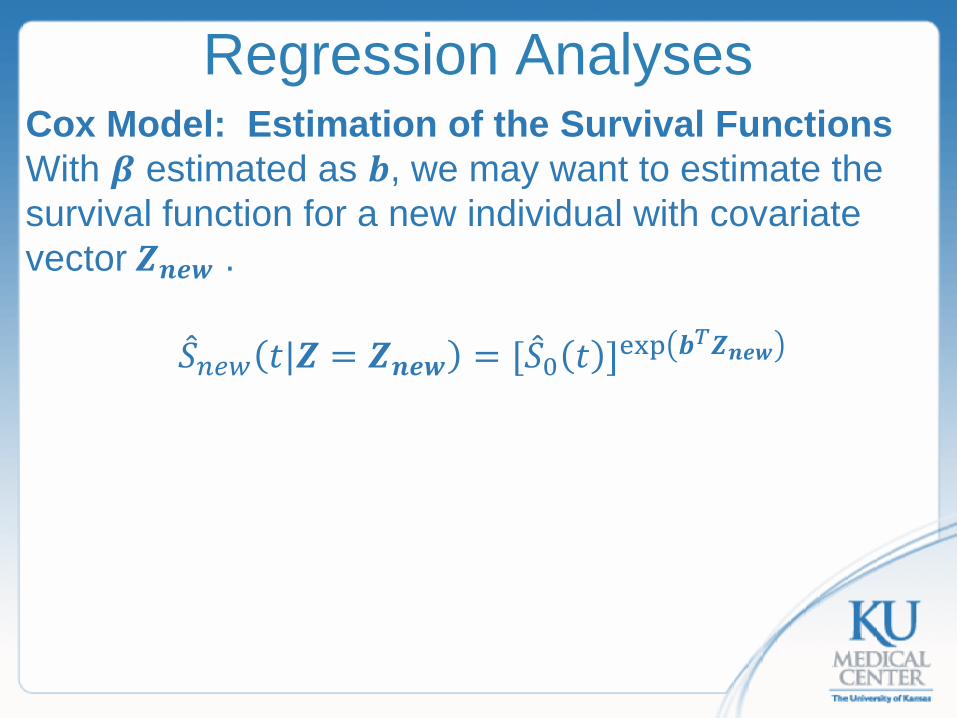
Regression Analyses Cox Model: Estimation of the Survival Functions With 𝜷𝜷 estimated as 𝒃𝒃, we may want to estimate the survival function for a new individual with covariate vector 𝒁𝒁𝒍𝒍𝒏𝒏𝒏𝒏 .
�̂�𝑆𝑛𝑛𝑎𝑎𝑤𝑤 𝑡𝑡|𝒁𝒁 = 𝒁𝒁𝒍𝒍𝒏𝒏𝒏𝒏 = [�̂�𝑆0 𝑡𝑡 ]exp 𝒃𝒃𝑇𝑇𝒁𝒁𝒍𝒍𝒏𝒏𝒏𝒏
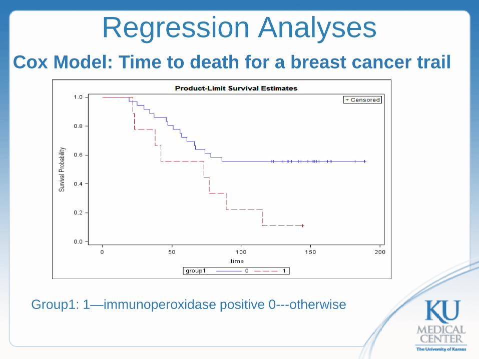
Regression Analyses Cox Model: Time to death for a breast cancer trail Group1: 1—immunoperoxidase positive 0---otherwise
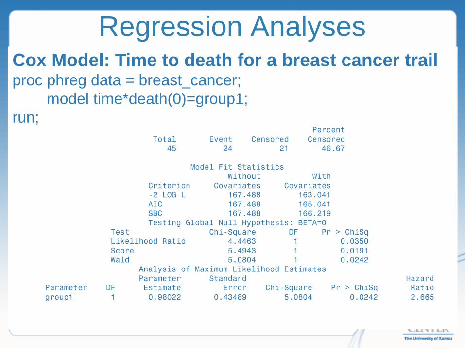
Regression Analyses Cox Model: Time to death for a breast cancer trail proc phreg data = breast_cancer; model time*death(0)=group1; run; Percent Total Event Censored Censored 45 24 21 46.67 Model Fit Statistics Without With Criterion Covariates Covariates -2 LOG L 167.488 163.041 AIC 167.488 165.041 SBC 167.488 166.219
Testing Global Null Hypothesis: BETA=0 Test Chi-Square DF Pr > ChiSq Likelihood Ratio 4.4463 1 0.0350 Score 5.4943 1 0.0191 Wald 5.0804 1 0.0242
Analysis of Maximum Likelihood Estimates Parameter Standard Hazard Parameter DF Estimate Error Chi-Square Pr > ChiSq Ratio group1 1 0.98022 0.43489 5.0804 0.0242 2.665

Regression Analyses Cox Model: Larynx Cancer proc phreg data=larynx; model time*death(0)=z1 z2 z3 age; run;
Parameter Standard Hazard Parameter DF Estimate Error Chi-Square Pr > ChiSq Ratio z1(stg II) 1 0.13842 0.46232 0.0896 0.7646 1.148 z2(stg III) 1 0.63815 0.35609 3.2116 0.0731 1.893 z3(stg IV) 1 1.69333 0.42218 16.0876 <.0001 5.438 age 1 0.01890 0.01425 1.7589 0.1848 1.019
The estimates of hazard ratios are similar to those from the exponential AFT model (HR=1.16, 1.91, and 5.12 for z1, z2, and z3, respectively).

Regression Analyses Cox Model: Ties proc phreg data=kidney ; model time*infect(0)= z1 /itprint; *default is Breslow’s method. run; Parameter Standard Hazard Parameter DF Estimate Error Chi-Square Pr > ChiSq Ratio z1 1 -0.61817 0.39813 2.4108 0.1205 0.539 proc phreg data=kidney; model time*infect(0)= z1 /ties = efron itprint; run; Parameter Standard Hazard Parameter DF Estimate Error Chi-Square Pr > ChiSq Ratio z1 1 -0.61257 0.39791 2.3699 0.1237 0.542 proc phreg data=kidney; model time*infect(0)= z1 /ties = discrete itprint; *use this is times are discrete run; Parameter Standard Hazard Parameter DF Estimate Error Chi-Square Pr > ChiSq Ratio z1 1 -0.62944 0.40190 2.4529 0.1173 0.533 proc phreg data=kidney; model time*infect(0)= z1 /ties = exact itprint; run; Parameter Standard Hazard Parameter DF Estimate Error Chi-Square Pr > ChiSq Ratio z1 1 -0.61265 0.39794 2.3703 0.1237 0.542
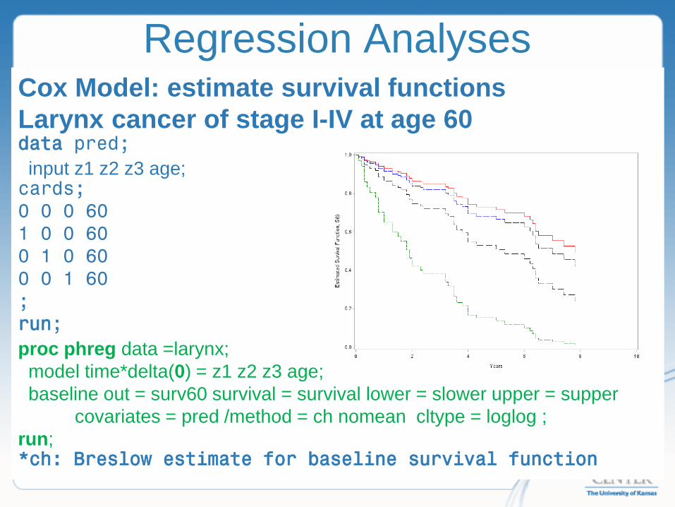
Regression Analyses Cox Model: estimate survival functions Larynx cancer of stage I-IV at age 60 data pred; input z1 z2 z3 age; cards; 0 0 0 60 1 0 0 60 0 1 0 60 0 0 1 60 ; run; proc phreg data =larynx; model time*delta(0) = z1 z2 z3 age; baseline out = surv60 survival = survival lower = slower upper = supper covariates = pred /method = ch nomean cltype = loglog ; run; *ch: Breslow estimate for baseline survival function
Regression Analyses Cox Model: Diagnosis Independent censoring—not testable with the given data (identifiability dilemma) Proportional hazards assumption

Regression Analyses Cox Model: Diagnosis 1. Assess the overall fit using Cox-Snell residuals 2. Identify the functional form of independent variable Z using Martingale residuals 3. Assess the proportional hazards assumption
Regression Analyses Cox Model: Diagnosis of overall fit Given data (𝑇𝑇𝑗𝑗 , 𝛿𝛿𝑗𝑗 , 𝑍𝑍𝑗𝑗(𝑡𝑡)) and a proportional hazards model
ℎ 𝑡𝑡 𝑍𝑍𝑗𝑗 𝑡𝑡 = ℎ0 𝑡𝑡 exp 𝜷𝜷𝑻𝑻𝒁𝒁𝑗𝑗 𝑡𝑡 , the distribution of 𝑆𝑆 𝑡𝑡 𝑍𝑍𝑗𝑗 𝑡𝑡 is uniform on [0,1] and the distribution of 𝐻𝐻 𝑡𝑡 𝑍𝑍𝑗𝑗 𝑡𝑡 = −ln(𝑆𝑆 𝑡𝑡 𝑍𝑍𝑗𝑗 𝑡𝑡 ] is censored exponential (1) if the model is correct.

Regression Analyses Cox Model: Diagnosis of overall fit Cox-Snell residuals
𝑑𝑑𝑗𝑗 = 𝐻𝐻�0 𝑇𝑇𝑗𝑗 exp(𝒃𝒃𝑇𝑇𝒁𝒁𝑗𝑗) , Where 𝐻𝐻�0 𝑇𝑇𝑗𝑗 is Breslow’s estimator of cumulative baseline hazard. Do these residuals behave like a sample from EXP(1)? The plot of 𝑑𝑑𝑗𝑗 vs the 𝐻𝐻�𝑁𝑁𝐴𝐴(𝑑𝑑𝑗𝑗) should be a straight line through the origin with a slope of 1, where 𝐻𝐻�𝑁𝑁𝐴𝐴(𝑑𝑑𝑗𝑗) is the Nelson-Aalen estimator of the cumulative hazard rate of using 𝑑𝑑𝑗𝑗𝜷s as survival times.
Regression Analyses Cox Model: Diagnosis of functional form Martingale residuals
𝑀𝑀�𝑗𝑗 = 𝑁𝑁𝑗𝑗 ∞ −� 𝑌𝑌𝑗𝑗 𝑡𝑡 exp[𝒃𝒃𝑻𝑻∞
0𝑍𝑍𝑗𝑗(𝑡𝑡)]𝑑𝑑𝐻𝐻�0(𝑡𝑡),
𝑗𝑗 = 1,2, … ,𝑛𝑛 When the data is right censored and all covariates are fixed at the baseline, the martingale residual reduces to
𝑀𝑀�𝑗𝑗 = 𝛿𝛿𝑗𝑗 − 𝑑𝑑𝑗𝑗 The martingale residuals are estimates of the excess number of events seen in the data but not predicted by the model.

Regression Analyses Cox Model: Diagnosis of functional form To find the functional form of a single variable 𝑍𝑍𝜷, we can fit a Cox model to the data based on other variables with known functional form and compute the martingale residuals, then plot the martingale residuals against 𝑍𝑍𝜷. The smoothed-fitted curve gives an indication of the functional form for 𝑍𝑍′.
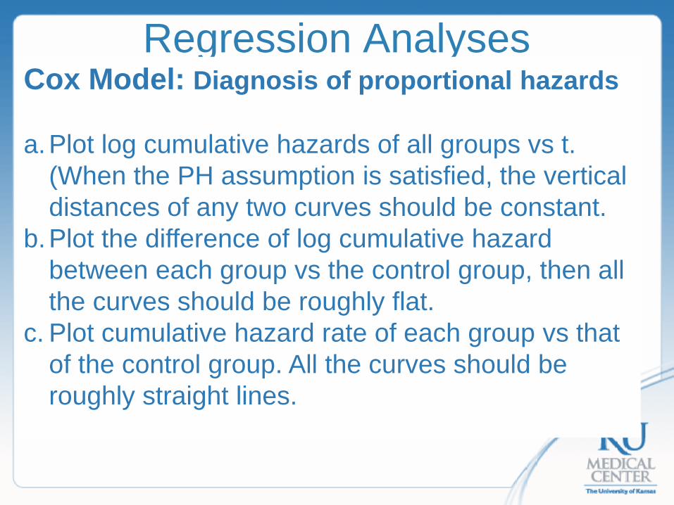
Regression Analyses Cox Model: Diagnosis of proportional hazards a.Plot log cumulative hazards of all groups vs t.
(When the PH assumption is satisfied, the vertical distances of any two curves should be constant.
b.Plot the difference of log cumulative hazard between each group vs the control group, then all the curves should be roughly flat.
c. Plot cumulative hazard rate of each group vs that of the control group. All the curves should be roughly straight lines.
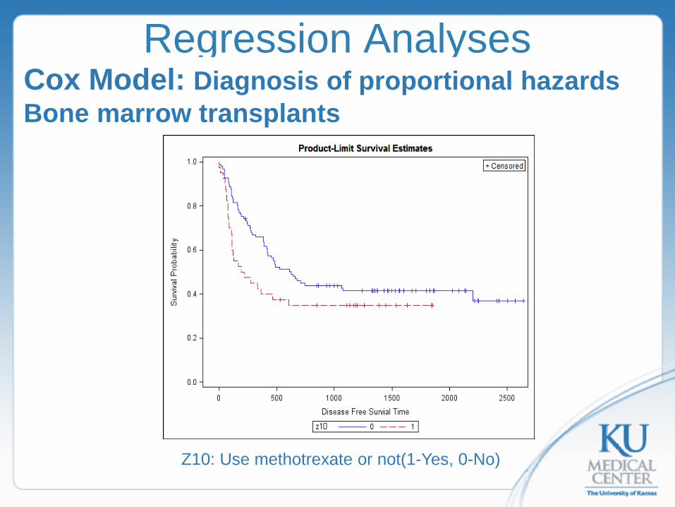
Regression Analyses Cox Model: Diagnosis of proportional hazards Bone marrow transplants
Z10: Use methotrexate or not(1-Yes, 0-No)

Regression Analyses Cox Model: Diagnosis of proportional hazards Bone marrow transplants

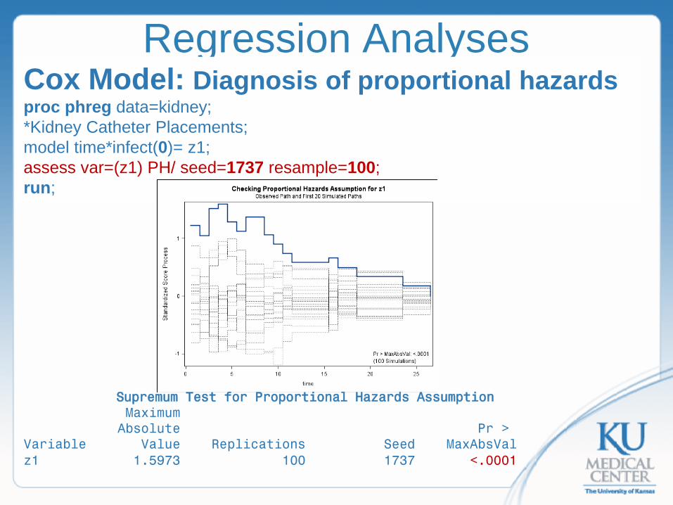
Regression Analyses Cox Model: Diagnosis of proportional hazards proc phreg data=kidney; *Kidney Catheter Placements; model time*infect(0)= z1; assess var=(z1) PH/ seed=1737 resample=100; run;
Supremum Test for Proportional Hazards Assumption Maximum Absolute Pr > Variable Value Replications Seed MaxAbsVal z1 1.5973 100 1737 <.0001
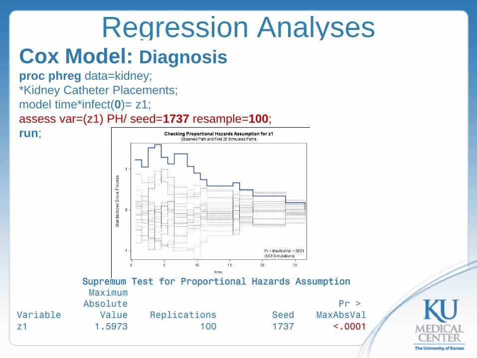
Regression Analyses Cox Model: Diagnosis proc phreg data=kidney; *Kidney Catheter Placements; model time*infect(0)= z1; assess var=(z1) PH/ seed=1737 resample=100; run;
Supremum Test for Proportional Hazards Assumption Maximum Absolute Pr > Variable Value Replications Seed MaxAbsVal z1 1.5973 100 1737 <.0001

Regression Analyses Cox Model: Diagnosis Outliers and Influential Observations by SAS DFBETA specifies the approximate changes in the parameter estimates �̂�𝛽 − �̂�𝛽(𝑗𝑗) when the j th observation is omitted. RESDEV specifies the deviance residual 𝐷𝐷�𝑗𝑗.This is a transform of the martingale residual to achieve a more symmetric distribution. RESMART specifies the martingale residual 𝑀𝑀�𝑗𝑗. XBETA specifies the estimate of the linear predictor 𝑋𝑋�̂�𝛽.
𝐷𝐷�𝑗𝑗 = 𝑙𝑙𝑖𝑖𝑔𝑔𝑛𝑛 𝑀𝑀�𝑗𝑗 {−2 𝑀𝑀�𝑗𝑗 + 𝛿𝛿𝑗𝑗 log 𝛿𝛿𝑗𝑗 − 𝑀𝑀�𝑗𝑗 }12, 𝐷𝐷�𝑗𝑗= 0 𝑖𝑖𝑓𝑓 𝑀𝑀�𝑗𝑗 = 0
To assess the effect of a given individual on the model, a plot of the deviance 𝐷𝐷�𝑗𝑗 vs risk score 𝑋𝑋�̂�𝛽 .When there is light to moderate censoring, the 𝐷𝐷�𝑗𝑗 should look like a sample of normally distributed noise. When there is heavy censoring, a large collections of points near zero will distort the normal approximation. In either case, potential outliers will have deviance residuals whose absolute values are too large. This part is similar to those for linear regression.
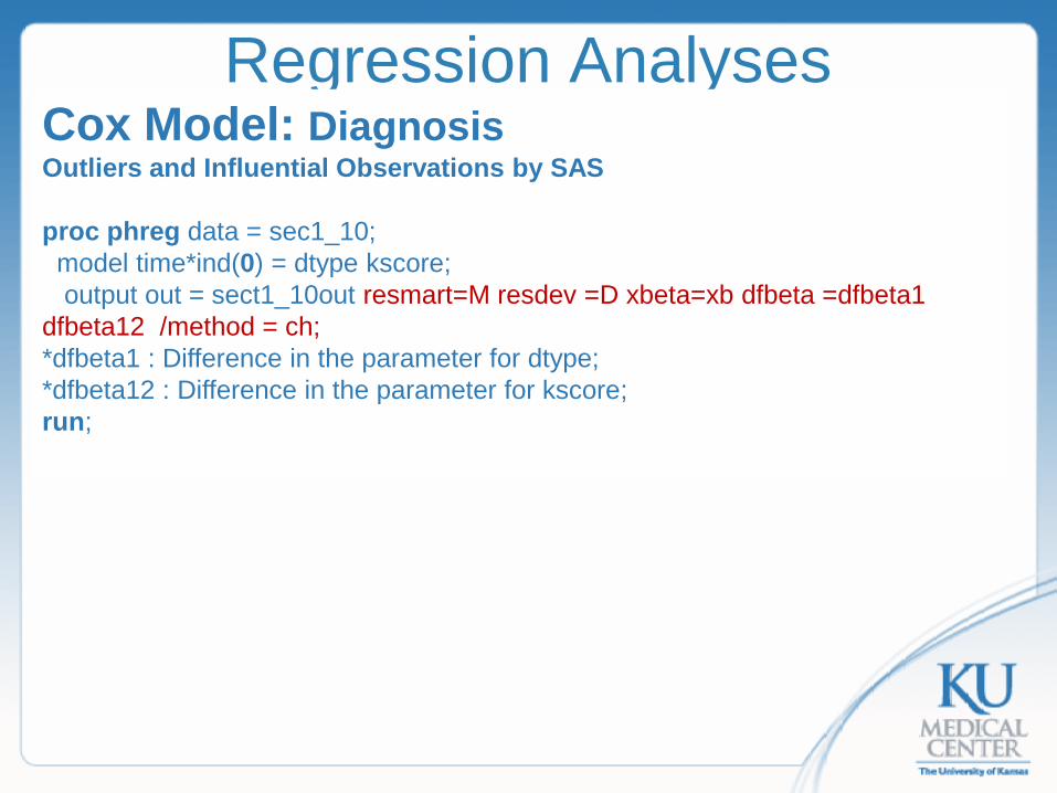
Regression Analyses Cox Model: Diagnosis Outliers and Influential Observations by SAS proc phreg data = sec1_10; model time*ind(0) = dtype kscore; output out = sect1_10out resmart=M resdev =D xbeta=xb dfbeta =dfbeta1 dfbeta12 /method = ch; *dfbeta1 : Difference in the parameter for dtype; *dfbeta12 : Difference in the parameter for kscore; run;
Regression Analyses Which time scale should we use, age or study time? It depends on the research interest and underlying survival functions. Some references Pencina, M. J., Larson, M. G., & D'Agostino, R. B. (2007). Choice of time scale and its effect on significance of predictors in longitudinal studies. Statistics in medicine, 26(6), 1343-1359. Kom, E. L., Graubard, B. I., & Midthune, D. (1997). Time-to-event analysis of longitudinal follow-up of a survey: choice of the time-scale. American journal of epidemiology, 145(1), 72-80. Thiébaut, A., & Bénichou, J. (2004). Choice of time‐scale in Cox's model analysis of epidemiologic cohort data: a simulation study. Statistics in medicine, 23(24),
3803-3820.
outline Introduction
• Time to event data /Censoring and truncation • Basic survival functions/Group comparison of survival
data
Regression Analyses • Parametric Approach -- Accelerated failure time
models • Semiparametric Approach – Cox models
Extension to the Cox models • Weighted Cox models: nonproportional hazards • Time-dependent covariate Cox models • Time-varying coefficient survival models
Other topics • Competing risk modeling • Bayesian survival analyses
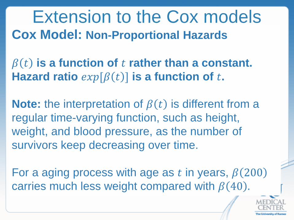
Extension to the Cox models Cox Model: Non-Proportional Hazards 𝛽𝛽 𝑡𝑡 is a function of 𝑡𝑡 rather than a constant. Hazard ratio 𝑒𝑒𝑥𝑥𝑝𝑝[𝛽𝛽 𝑡𝑡 ] is a function of 𝑡𝑡. Note: the interpretation of 𝛽𝛽 𝑡𝑡 is different from a regular time-varying function, such as height, weight, and blood pressure, as the number of survivors keep decreasing over time. For a aging process with age as 𝑡𝑡 in years, 𝛽𝛽 200 carries much less weight compared with 𝛽𝛽 40 .
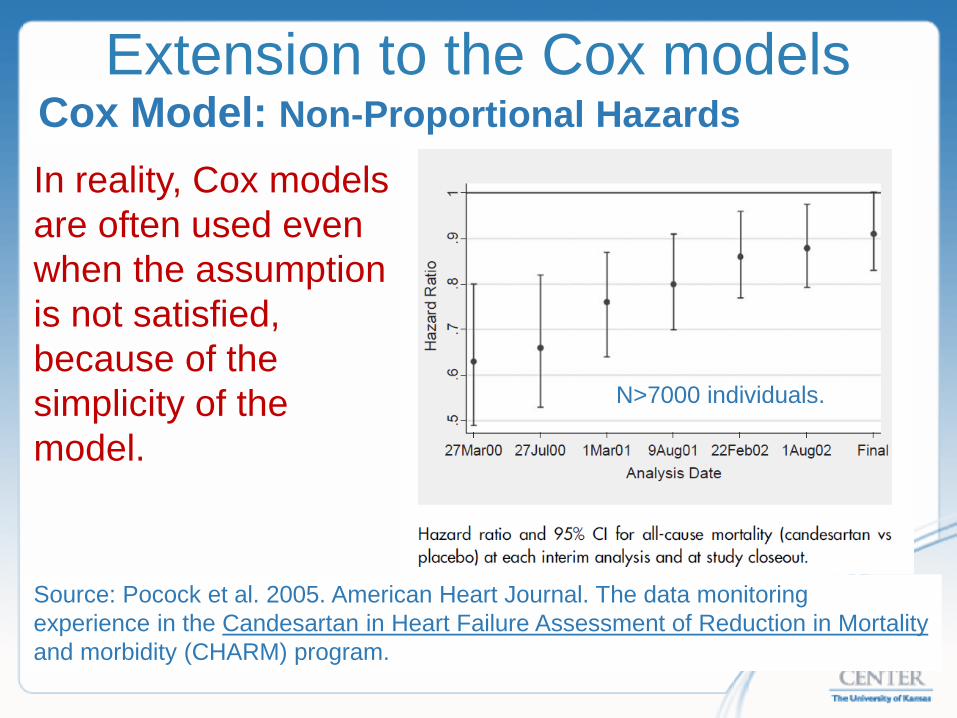
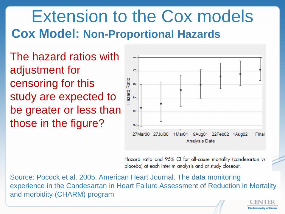
Extension to the Cox models Cox Model: Non-Proportional Hazards
Source: Pocock et al. 2005. American Heart Journal. The data monitoring experience in the Candesartan in Heart Failure Assessment of Reduction in Mortality and morbidity (CHARM) program.
In reality, Cox models are often used even when the assumption is not satisfied, because of the simplicity of the model.
N>7000 individuals.
Extension to the Cox models
Can we use the Cox model when the proportional hazards assumption is violated? What is the interpretation? Any issue we should be aware of?
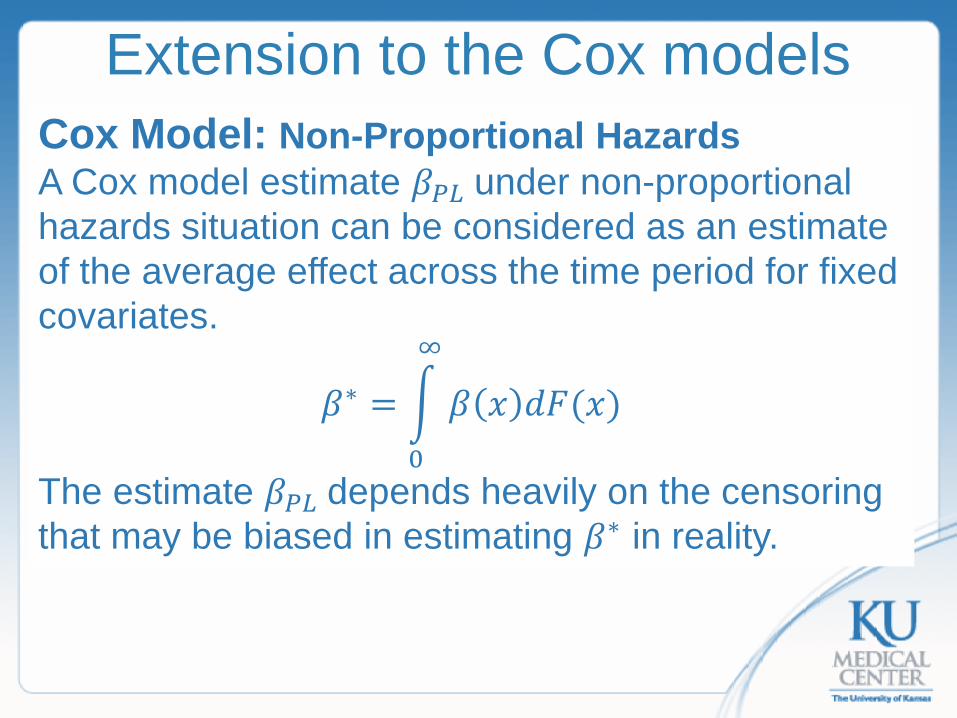
Extension to the Cox models Cox Model: Non-Proportional Hazards A Cox model estimate 𝛽𝛽𝑃𝑃𝐿𝐿 under non-proportional hazards situation can be considered as an estimate of the average effect across the time period for fixed covariates.
𝛽𝛽∗ = � 𝛽𝛽 𝑥𝑥 𝑑𝑑𝐹𝐹(𝑥𝑥)∞
0
The estimate 𝛽𝛽𝑃𝑃𝐿𝐿 depends heavily on the censoring that may be biased in estimating 𝛽𝛽∗ in reality.
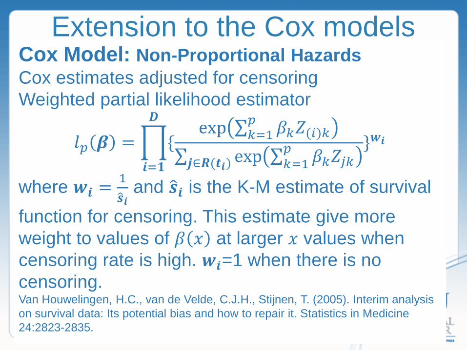
Extension to the Cox models Cox Model: Non-Proportional Hazards Cox estimates adjusted for censoring Weighted partial likelihood estimator
𝑙𝑙𝑝𝑝 𝜷𝜷 = �{exp ∑ 𝛽𝛽𝑘𝑘𝑍𝑍(𝑖𝑖)𝑘𝑘
𝑝𝑝𝑘𝑘=1
∑ exp ∑ 𝛽𝛽𝑘𝑘𝑍𝑍𝑗𝑗𝑘𝑘𝑝𝑝𝑘𝑘=1𝒋𝒋∈𝑹𝑹(𝒕𝒕𝒊𝒊)
𝑫𝑫
𝒊𝒊=𝟏𝟏
}𝒏𝒏𝒊𝒊
where 𝒏𝒏𝒊𝒊 = 1𝒔𝒔�𝒊𝒊
and 𝒔𝒔�𝒊𝒊 is the K-M estimate of survival function for censoring. This estimate give more weight to values of 𝛽𝛽 𝑥𝑥 at larger 𝑥𝑥 values when censoring rate is high. 𝒏𝒏𝒊𝒊=1 when there is no censoring. Van Houwelingen, H.C., van de Velde, C.J.H., Stijnen, T. (2005). Interim analysis on survival data: Its potential bias and how to repair it. Statistics in Medicine 24:2823-2835.

Extension to the Cox models Cox Model: Non-Proportional Hazards BDP data
0.00
0.25
0.50
0.75
1.00
0 200 400 600 800day
No SRT SRT
Kaplan-Meier survival estimates
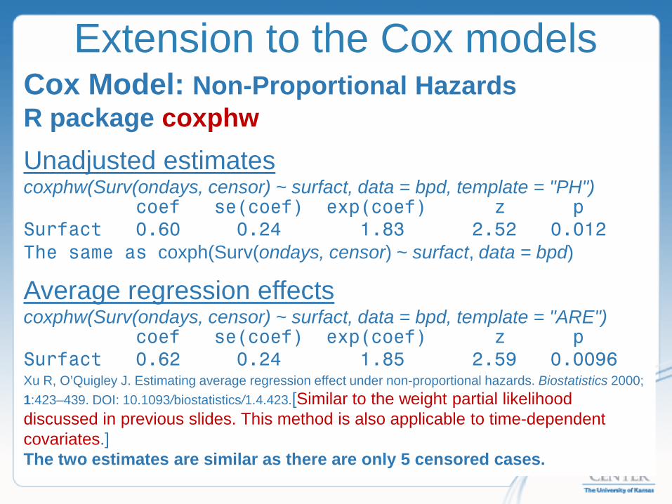
Extension to the Cox models Cox Model: Non-Proportional Hazards R package coxphw
Unadjusted estimates coxphw(Surv(ondays, censor) ~ surfact, data = bpd, template = "PH") coef se(coef) exp(coef) z p Surfact 0.60 0.24 1.83 2.52 0.012 The same as coxph(Surv(ondays, censor) ~ surfact, data = bpd)
Average regression effects coxphw(Surv(ondays, censor) ~ surfact, data = bpd, template = "ARE") coef se(coef) exp(coef) z p Surfact 0.62 0.24 1.85 2.59 0.0096 Xu R, O’Quigley J. Estimating average regression effect under non-proportional hazards. Biostatistics 2000; 1:423–439. DOI: 10.1093/biostatistics/1.4.423.[Similar to the weight partial likelihood discussed in previous slides. This method is also applicable to time-dependent covariates.] The two estimates are similar as there are only 5 censored cases.

Extension to the Cox models Cox Model: Non-Proportional Hazards R package coxphw Average hazard ratios (default) coxphw(formula = Surv(ondays, censor) ~ surfact, data = data) coef se(coef) exp(coef) z p surfact 0.44 0.26 1.56 1.68 0.094 Schemper M, Wakounig S, Heinze G. The estimation of average hazard ratios by weighted Cox regression. Statistics in Medicine 2009;28(19):2473--2489.
Note: this estimate is very different from Cox estimate without censoring.
Extension to the Cox models Cox Model: Non-Proportional Hazards
Source: Pocock et al. 2005. American Heart Journal. The data monitoring experience in the Candesartan in Heart Failure Assessment of Reduction in Mortality and morbidity (CHARM) program
The hazard ratios with adjustment for censoring for this study are expected to be greater or less than those in the figure?

Regression Analyses Cox Model: time-dependent covariates Covariate Z may change with time Z(t) Using time-dependent covariates Cox model to A: test the impact of intermediate events B: test the proportional hazards assumption
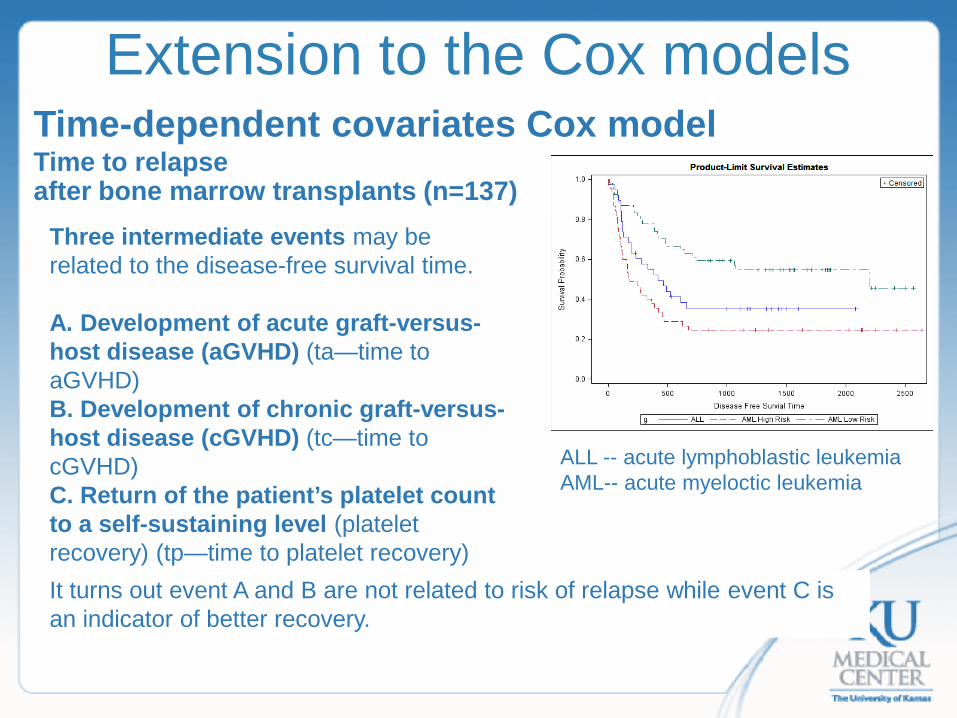
Extension to the Cox models Time-dependent covariates Cox model Time to relapse after bone marrow transplants (n=137)
ALL -- acute lymphoblastic leukemia AML-- acute myeloctic leukemia
Three intermediate events may be related to the disease-free survival time. A. Development of acute graft-versus-host disease (aGVHD) (ta—time to aGVHD) B. Development of chronic graft-versus-host disease (cGVHD) (tc—time to cGVHD) C. Return of the patient’s platelet count to a self-sustaining level (platelet recovery) (tp—time to platelet recovery) It turns out event A and B are not related to risk of relapse while event C is an indicator of better recovery.
Extension to the Cox models Time-dependent covariates Cox model This model provides a simple way of modeling time-varying effect of covariates with their proportional hazards assumptions violated.
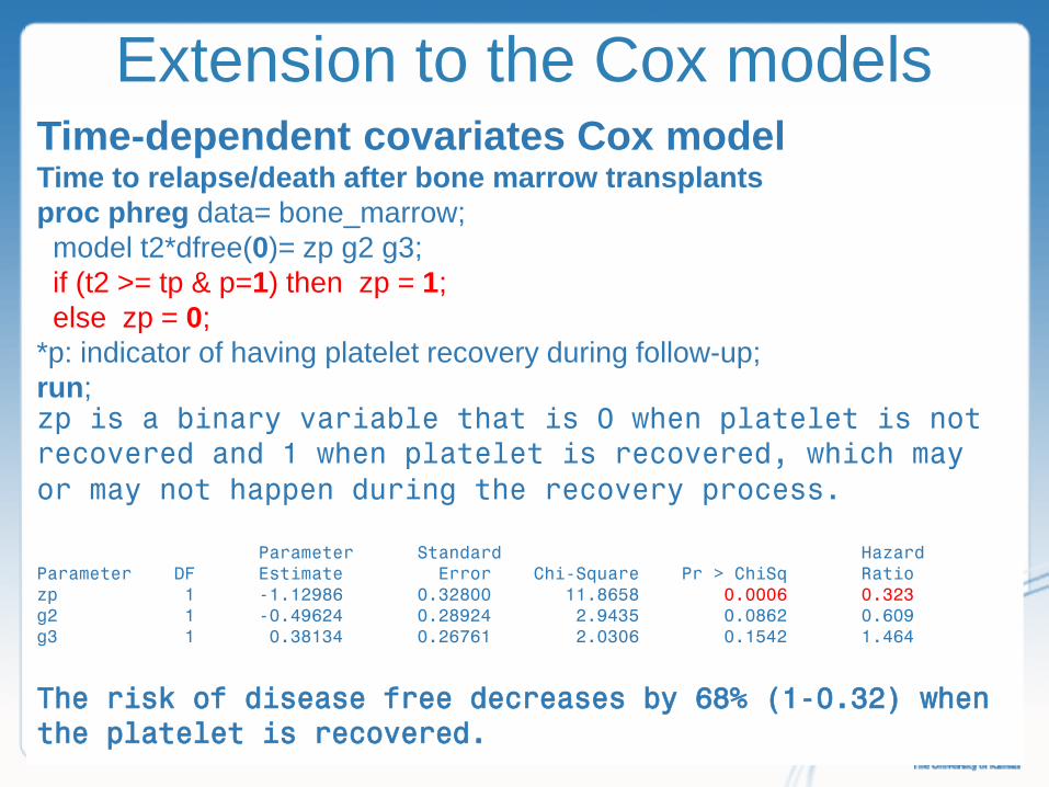
Extension to the Cox models Time-dependent covariates Cox model Time to relapse/death after bone marrow transplants proc phreg data= bone_marrow; model t2*dfree(0)= zp g2 g3; if (t2 >= tp & p=1) then zp = 1; else zp = 0; *p: indicator of having platelet recovery during follow-up; run; zp is a binary variable that is 0 when platelet is not recovered and 1 when platelet is recovered, which may or may not happen during the recovery process. Parameter Standard Hazard Parameter DF Estimate Error Chi-Square Pr > ChiSq Ratio zp 1 -1.12986 0.32800 11.8658 0.0006 0.323 g2 1 -0.49624 0.28924 2.9435 0.0862 0.609 g3 1 0.38134 0.26761 2.0306 0.1542 1.464
The risk of disease free decreases by 68% (1-0.32) when the platelet is recovered.

Extension to the Cox models Time-dependent covariates Cox model Time to infection of kidney dialysis patients The survival functions of the two treatment cross each other, suggesting the infection risk for surgical patients maybe higher at first, but it becomes lower after about 5 months. This is an indicator of possible violation of the proportional hazards assumption. proc phreg data=kidney1; model time*infect(0)= z1 Z1t; z1t=z1*time; run; Parameter Standard Hazard Parameter DF Estimate Error Chi-Square Pr > ChiSq Ratio z1 1 0.94335 0.75154 1.5756 0.2094 2.569 Z1t 1 -0.25343 0.11695 4.6955 0.0302 0.776
The hazard ratio of percutaneous/surgical decreases with time. b (t) =ln[hr(t)] =0.94335-0.25343t HR(t)=2.569*(0.776)t. HR(t)=1 when t=3.7 months.
0= "surgical" 1 = "percutaneous"

Extension to the Cox models Time-dependent covariates Cox model Application: Body weight and mortality The association of body weight measured by body mass index (BMI=weight (kg)/height2 (m2)) and all-cause mortality has been reported to have different shapes. Traditional Cox model or logistic regression models were used.
BMI
No association
U-shaped
J-shaped
Direct
Inverse
*Risk can be measured as relative risk, odds ratio, and hazard ratio etc.
Ris
k of
dea
th*
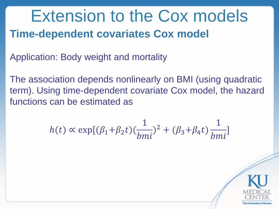
Extension to the Cox models Time-dependent covariates Cox model Application: Body weight and mortality The association depends nonlinearly on BMI (using quadratic term). Using time-dependent covariate Cox model, the hazard functions can be estimated as
ℎ(𝑡𝑡) ∝ exp[(𝛽𝛽1+𝛽𝛽2𝑡𝑡)(1𝑊𝑊𝑠𝑠𝑖𝑖
)2 + (𝛽𝛽3+𝛽𝛽4𝑡𝑡)1𝑊𝑊𝑠𝑠𝑖𝑖
]
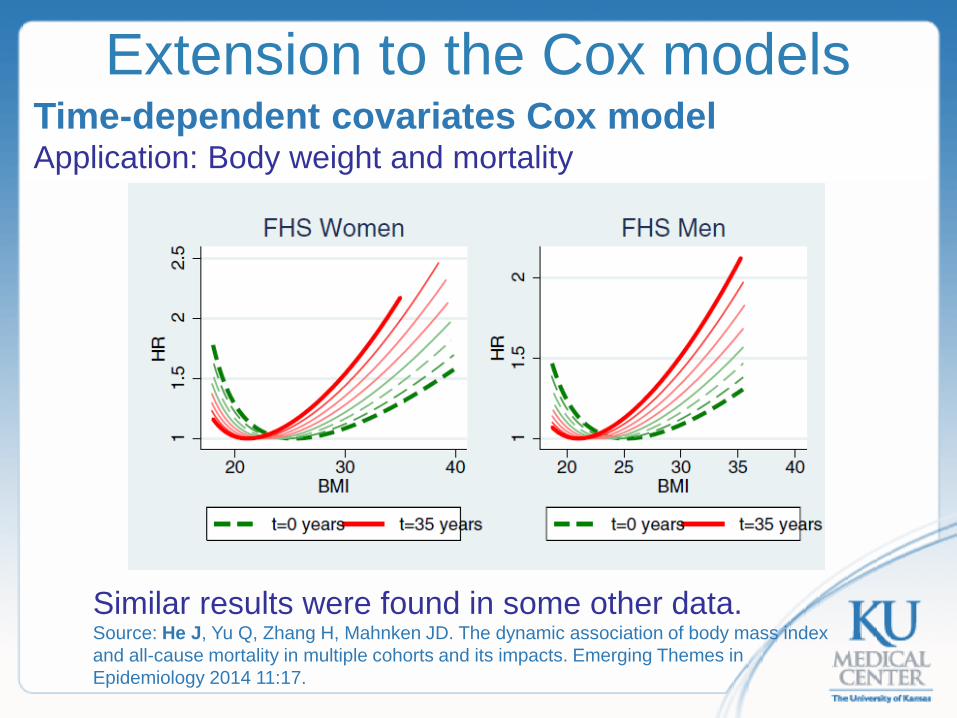
Extension to the Cox models Time-dependent covariates Cox model Application: Body weight and mortality
Similar results were found in some other data. Source: He J, Yu Q, Zhang H, Mahnken JD. The dynamic association of body mass index and all-cause mortality in multiple cohorts and its impacts. Emerging Themes in Epidemiology 2014 11:17.

Extension to the Cox models Time-dependent covariates Cox model Application: Body weight and mortality Conclusion: Because the association changes with time that studies with different lengths of follow-up may naturally obtain different results as their estimates using traditional Cox model were averages effects within different time period. Short studies tend to obtained inverse associations. This finding is consistent with the fact that most studies obtained inverse associations have follow-up lengths shorter than 10 years.
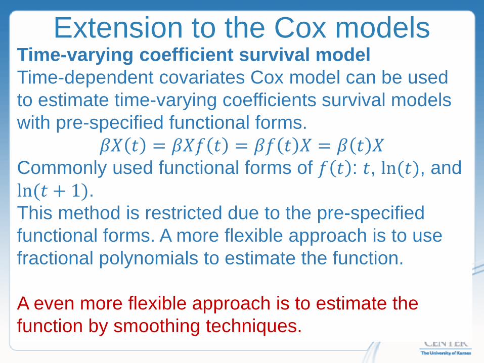
Extension to the Cox models Time-varying coefficient survival model Time-dependent covariates Cox model can be used to estimate time-varying coefficients survival models with pre-specified functional forms.
𝛽𝛽𝑋𝑋 𝑡𝑡 = 𝛽𝛽𝑋𝑋𝑓𝑓 𝑡𝑡 = 𝛽𝛽𝑓𝑓 𝑡𝑡 𝑋𝑋 = 𝛽𝛽 𝑡𝑡 𝑋𝑋 Commonly used functional forms of 𝑓𝑓 𝑡𝑡 : 𝑡𝑡, ln(𝑡𝑡), and ln(𝑡𝑡 + 1). This method is restricted due to the pre-specified functional forms. A more flexible approach is to use fractional polynomials to estimate the function. A even more flexible approach is to estimate the function by smoothing techniques.
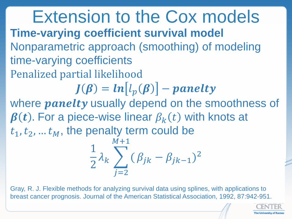
Extension to the Cox models Time-varying coefficient survival model Nonparametric approach (smoothing) of modeling time-varying coefficients Penalized partial likelihood
𝑱𝑱 𝜷𝜷 = 𝒂𝒂𝒍𝒍 𝑙𝑙𝑝𝑝 𝜷𝜷 − 𝒑𝒑𝒂𝒂𝒍𝒍𝒏𝒏𝒂𝒂𝒕𝒕𝒑𝒑 where 𝒑𝒑𝒂𝒂𝒍𝒍𝒏𝒏𝒂𝒂𝒕𝒕𝒑𝒑 usually depend on the smoothness of 𝜷𝜷 𝒕𝒕 . For a piece-wise linear 𝛽𝛽𝑘𝑘 𝑡𝑡 with knots at 𝑡𝑡1, 𝑡𝑡2, … 𝑡𝑡𝑀𝑀, the penalty term could be
12𝜆𝜆𝑘𝑘 � (
𝑀𝑀+1
𝑗𝑗=2
𝛽𝛽𝑗𝑗𝑘𝑘 − 𝛽𝛽𝑗𝑗𝑘𝑘−1)2
Gray, R. J. Flexible methods for analyzing survival data using splines, with applications to breast cancer prognosis. Journal of the American Statistical Association, 1992, 87:942-951.
Extension to the Cox models Time-varying coefficient survival model Nonparametric approach (smoothing) of modeling time-varying coefficients R package coxspline by Gray (panelized B-splines) http://biowww.dfci.harvard.edu/~gray/ May not be compatible with the latest R. R function splineCox in package dynsurv (CRAN) by Wang, Yan, and Chen. A tutorial is available at http://cran.r-project.org/web/packages/dynsurv/dynsurv.pdf
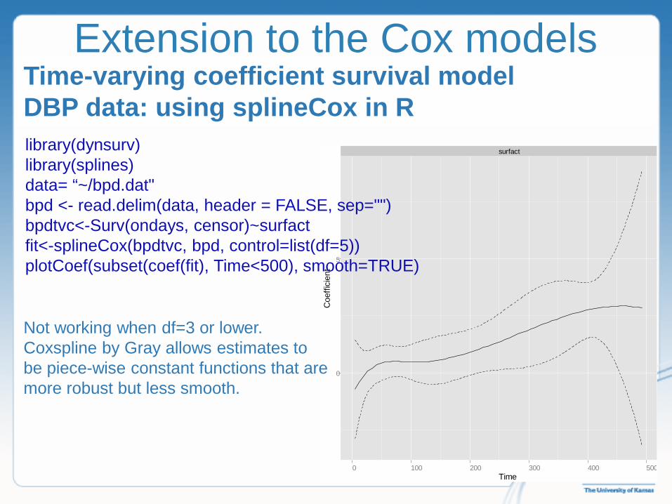
Extension to the Cox models Time-varying coefficient survival model DBP data: using splineCox in R
surfact
0
5
0 100 200 300 400 500Time
Coe
ffici
ent
library(dynsurv) library(splines) data= “~/bpd.dat" bpd <- read.delim(data, header = FALSE, sep="") bpdtvc<-Surv(ondays, censor)~surfact fit<-splineCox(bpdtvc, bpd, control=list(df=5)) plotCoef(subset(coef(fit), Time<500), smooth=TRUE)
Not working when df=3 or lower. Coxspline by Gray allows estimates to be piece-wise constant functions that are more robust but less smooth.
Extension to the Cox models Time-varying coefficient survival model Bayesian approach can be use to estimate time-varying coefficient models using Bayesian smoothing techniques, see the next section about Bayesian survival models.

Outline Introduction
• Time to event data /Censoring and truncation • Basic survival functions/Group comparison of survival
data
Regression Analyses • Parametric Approach -- Accelerated failure time
models • Semiparametric Approach – Cox models
Extension to the Cox models • Weighted Cox models • Time-dependent covariate Cox models • Time-varying coefficient survival models
Other topics • Competing risk modeling • Bayesian survival analyses
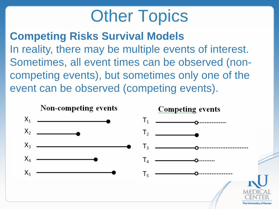
Other Topics Competing Risks Survival Models In reality, there may be multiple events of interest. Sometimes, all event times can be observed (non-competing events), but sometimes only one of the event can be observed (competing events).

Other Topics Competing Risks Survival Models Let 𝑋𝑋𝑖𝑖, 𝑖𝑖 = 1, … ,𝐾𝐾 be the competing event times. 𝑇𝑇 = Min(X1, … , X𝐾𝐾) is observed event time and δ indicates which of the K events happens first. δ = i if T = X𝑖𝑖. Cause-specific (crude) hazard rate
ℎ𝑖𝑖𝑐𝑐 𝑡𝑡 = lim
∆𝑡𝑡→0
𝑃𝑃(𝑡𝑡 ≤ 𝑇𝑇 < 𝑡𝑡 + ∆𝑡𝑡, δ = i |𝑇𝑇 ≥ 𝑡𝑡)∆𝑡𝑡
ℎ𝑖𝑖𝑐𝑐 𝑡𝑡 measures the instantaneous risk of having an
i event for a subject who hasn’t experienced any of the K events at time t, that is, the risk of observing event 𝑖𝑖 happening first.

Other Topics Competing Risks Survival Models The overall hazard rate of the time to failure(any of the competing events happening), T, is
ℎ𝑇𝑇 𝑡𝑡 = �ℎ𝑖𝑖𝑐𝑐 𝑡𝑡𝐾𝐾
𝑖𝑖=1
For example, all-cause mortality can be considered as the combination of mortalities of multiple mutually exclusive causes, such as, cancer-related, car accidents, murder,…etc.

Other Topics Competing Risks Survival Models Cumulative Incidence Function (CIF)
𝐶𝐶𝐼𝐼𝐹𝐹𝑖𝑖 𝑡𝑡 = 𝑃𝑃 𝑇𝑇 ≤ 𝑡𝑡, 𝛿𝛿 = 𝑖𝑖 = � ℎ𝑖𝑖𝑐𝑐 𝜇𝜇 exp{−𝐻𝐻𝑇𝑇
𝑡𝑡
0(𝜇𝜇)}𝑑𝑑𝜇𝜇
When all competing events are independent, ℎ𝑖𝑖𝑐𝑐 𝜇𝜇 is the same as marginal ℎ𝑖𝑖 𝜇𝜇 that is estimable using the regular Cox model assuming a single event of interest and other events are censoring. However, the independent assumption cannot be tested statistically and may not be reasonable from the clinical aspect. Further more, the effect of covariates is not directly associated with CIF.
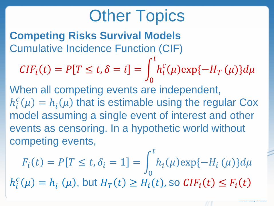
Other Topics Competing Risks Survival Models Cumulative Incidence Function (CIF)
𝐶𝐶𝐼𝐼𝐹𝐹𝑖𝑖 𝑡𝑡 = 𝑃𝑃 𝑇𝑇 ≤ 𝑡𝑡, 𝛿𝛿 = 𝑖𝑖 = � ℎ𝑖𝑖𝑐𝑐 𝜇𝜇 exp{−𝐻𝐻𝑇𝑇
𝑡𝑡
0(𝜇𝜇)}𝑑𝑑𝜇𝜇
When all competing events are independent, ℎ𝑖𝑖𝑐𝑐 𝜇𝜇 = ℎ𝑖𝑖 𝜇𝜇 that is estimable using the regular Cox model assuming a single event of interest and other events as censoring. In a hypothetic world without competing events,
𝐹𝐹𝑖𝑖 𝑡𝑡 = 𝑃𝑃 𝑇𝑇 ≤ 𝑡𝑡, 𝛿𝛿𝑖𝑖 = 1 = � ℎ𝑖𝑖 𝜇𝜇 exp {−𝐻𝐻𝑖𝑖𝑡𝑡
0(𝜇𝜇)}𝑑𝑑𝜇𝜇
ℎ𝑖𝑖𝑐𝑐 𝜇𝜇 = ℎ𝑖𝑖 𝜇𝜇 , but 𝐻𝐻𝑇𝑇 𝑡𝑡 ≥ 𝐻𝐻𝑖𝑖(𝑡𝑡), so 𝐶𝐶𝐼𝐼𝐹𝐹𝑖𝑖 𝑡𝑡 ≤ 𝐹𝐹𝑖𝑖 𝑡𝑡

Other Topics Competing Risks Survival Models Cause-specific hazard regression model
ℎ𝑖𝑖𝑐𝑐 𝜇𝜇 = ℎ𝑖𝑖 𝜇𝜇 = ℎ𝑖𝑖0 𝜇𝜇 exp (𝜷𝜷′𝑿𝑿)
𝐶𝐶𝐼𝐼𝐹𝐹𝑖𝑖 = � ℎ𝑖𝑖𝑐𝑐 𝜇𝜇 exp{−𝐻𝐻𝑇𝑇𝑡𝑡
0(𝜇𝜇)}𝑑𝑑𝜇𝜇
This model is based on the independence assumption that cannot be tested statistically and may not be reasonable from the clinical aspect. For example, death due to coronary heart disease and death due to stroke are likely to be related. Further more, the effect of covariates is not directly associated with CIF (observable outcomes).
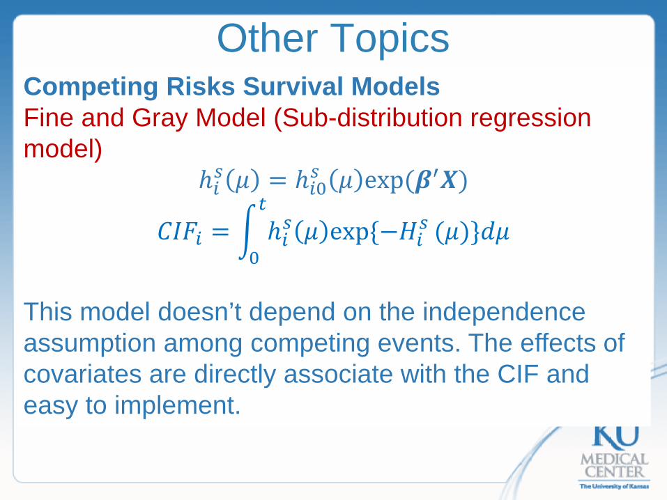
Other Topics Competing Risks Survival Models Fine and Gray Model (Sub-distribution regression model)
ℎ𝑖𝑖𝑠𝑠 𝜇𝜇 = ℎ𝑖𝑖0𝑠𝑠 𝜇𝜇 exp (𝜷𝜷′𝑿𝑿)
𝐶𝐶𝐼𝐼𝐹𝐹𝑖𝑖 = � ℎ𝑖𝑖𝑠𝑠 𝜇𝜇 exp{−𝐻𝐻𝑖𝑖𝑠𝑠𝑡𝑡
0(𝜇𝜇)}𝑑𝑑𝜇𝜇
This model doesn’t depend on the independence assumption among competing events. The effects of covariates are directly associate with the CIF and easy to implement.
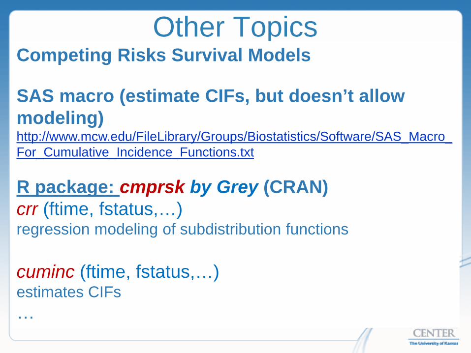
Other Topics Competing Risks Survival Models SAS macro (estimate CIFs, but doesn’t allow modeling) http://www.mcw.edu/FileLibrary/Groups/Biostatistics/Software/SAS_Macro_For_Cumulative_Incidence_Functions.txt R package: cmprsk by Grey (CRAN) crr (ftime, fstatus,…) regression modeling of subdistribution functions cuminc (ftime, fstatus,…) estimates CIFs …
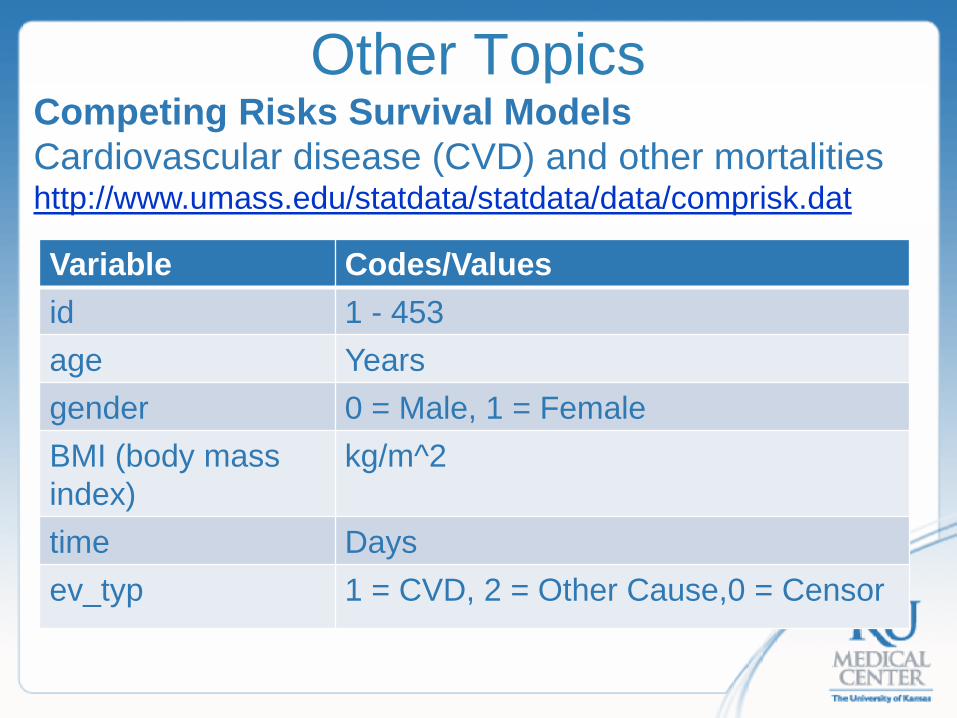
Other Topics Competing Risks Survival Models Cardiovascular disease (CVD) and other mortalities http://www.umass.edu/statdata/statdata/data/comprisk.dat
Variable Codes/Values id 1 - 453 age Years gender 0 = Male, 1 = Female BMI (body mass index)
kg/m^2
time Days ev_typ 1 = CVD, 2 = Other Cause,0 = Censor
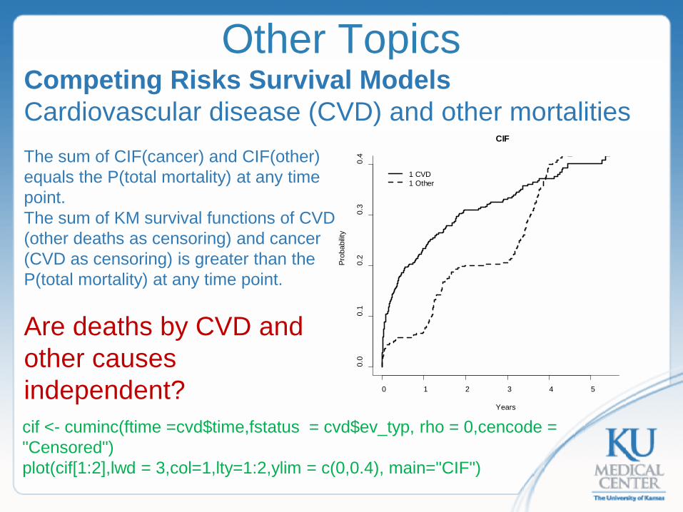
Other Topics Competing Risks Survival Models Cardiovascular disease (CVD) and other mortalities
cif <- cuminc(ftime =cvd$time,fstatus = cvd$ev_typ, rho = 0,cencode = "Censored") plot(cif[1:2],lwd = 3,col=1,lty=1:2,ylim = c(0,0.4), main="CIF")
0 1 2 3 4 5
0.0
0.1
0.2
0.3
0.4
CIF
Years
Prob
abilit
y
1 CVD1 Other
The sum of CIF(cancer) and CIF(other) equals the P(total mortality) at any time point. The sum of KM survival functions of CVD (other deaths as censoring) and cancer (CVD as censoring) is greater than the P(total mortality) at any time point.
Are deaths by CVD and other causes independent?

Other Topics Competing Risks Survival Models CVD Mortality-- Fine and Gray model
coef exp(coef) se(coef) z p-value Female -0.0752 0.928 0.1640 -0.459 0.650 Underweight -1.3686 0.254 1.0364 -1.320 0.190 Overweight 0.4465 1.563 0.2387 1.870 0.061 Obese 0.7078 2.029 0.2290 3.091 0.002 age 0.0890 1.093 0.0069 12.886 0.000 finegray <- crr(ftime =cvd$time,fstatus = cvd$ev_typ, cov1=x,failcode ="Cancer", cencode = "Censored")
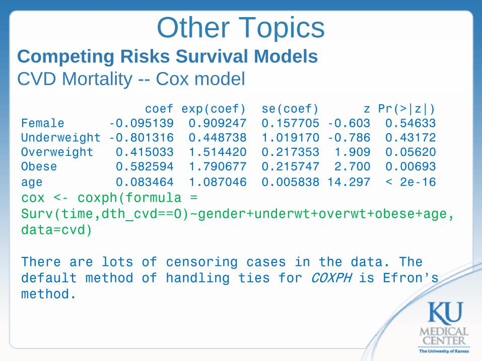
Other Topics Competing Risks Survival Models CVD Mortality -- Cox model coef exp(coef) se(coef) z Pr(>|z|) Female -0.095139 0.909247 0.157705 -0.603 0.54633 Underweight -0.801316 0.448738 1.019170 -0.786 0.43172 Overweight 0.415033 1.514420 0.217353 1.909 0.05620 Obese 0.582594 1.790677 0.215747 2.700 0.00693 age 0.083464 1.087046 0.005838 14.297 < 2e-16 cox <- coxph(formula = Surv(time,dth_cvd==0)~gender+underwt+overwt+obese+age, data=cvd) There are lots of censoring cases in the data. The default method of handling ties for COXPH is Efron’s method.
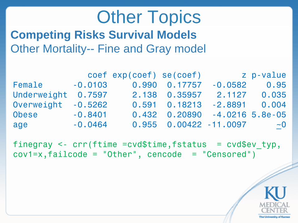
Other Topics Competing Risks Survival Models Other Mortality-- Fine and Gray model
coef exp(coef) se(coef) z p-value Female -0.0103 0.990 0.17757 -0.0582 0.95 Underweight 0.7597 2.138 0.35957 2.1127 0.035 Overweight -0.5262 0.591 0.18213 -2.8891 0.004 Obese -0.8401 0.432 0.20890 -4.0216 5.8e-05 age -0.0464 0.955 0.00422 -11.0097 ~0 finegray <- crr(ftime =cvd$time,fstatus = cvd$ev_typ, cov1=x,failcode = "Other", cencode = "Censored")

Other Topics Competing Risks Survival Models Other Mortality -- Cox model coef exp(coef) se(coef) z Pr(>|z|) Female -0.008966 0.991074 0.178794 -0.050 0.96000 underwt 0.718968 2.052315 0.308726 2.329 0.01987 overwt -0.335500 0.714980 0.182532 -1.838 0.06606 obese -0.621722 0.537019 0.220110 -2.825 0.00473 age -0.027848 0.972536 0.004893 -5.691 1.26e-08 cox <- coxph(formula = Surv(time,dth_cvd==0)~gender+underwt+overwt+obese+age, data=cvd)
Other Topics Bayesian Survival Analysis With the development of computation techniques, Bayesian methods are used more and more common. For Bayesian analysis, all parameters are considered as random variables rather than constant (frequentist). Given prior distributions of parameters, posterior distributions parameters can be obtained. Bayes’ theorem
𝑝𝑝 𝜃𝜃 𝑇𝑇 =𝑝𝑝 𝑇𝑇 𝜃𝜃 𝑝𝑝(𝜃𝜃)
𝑝𝑝(𝑇𝑇)~𝑝𝑝 𝑇𝑇 𝜃𝜃 𝑝𝑝(𝜃𝜃)
Other Topics Bayesian Survival Analysis Bayesian approach is very useful When there are strong prior distributions based on
expert opinions or data from previous studies. When the model is very complex that numeric
solutions based on likelihoods are difficult. Bayesian models can use sampling methods (MCMC) to obtain samples from the posterior distribution of parameter.

Other Topics Bayesian Survival Analysis In SAS, both PROC LIFEREG and PROC PHREG have the Bayes option that provide Bayesian estimates. Unless informative priors are provided, the results are similar to those of frequentist's approaches. ODS graphics on; proc phreg data=bpd; model ondays*censor(0)=surfact; bayes seed=23855 NBI=10000 NMC=50000 thinning=10 outpost=Post DIAGNOSTICS=ALL PLOTS=(trace autocorr); run; ods graphics off;
Other Topics Bayesian Survival Analysis Bayesian survival analysis is more useful in estimating more complicated models than regular AFT and Cox model. Researchers often need to write their own codes. Reference book: Bayesian Survival Analysis By Ibrahim, Joseph G., Chen, Ming-Hui, Sinha, Debajyoti.

Other Topics Frailty model using proc PHREG (Random Effects) https://www.youtube.com/watch?v=ZfgRBuM4u3U Multi-state models R package: mstate
Related Documents