Antarctic ice growth before and after the Eocene …environment.harvard.edu/sites/default/files/152._antarctic_ice... · Antarctic ice growth before and after the Eocene-Oligocene

Antarctic ice growth before and after the Eocene-Oligocenetransition: New estimates from clumped isotopepaleothermometryS. V. Petersen1,2 and D. P. Schrag1

1Department of Earth and Planetary Sciences, Harvard University, Cambridge, Massachusetts, USA, 2Now at Department ofEarth and Environmental Sciences, University of Michigan, Ann Arbor, Michigan, USA

Abstract Across the Eocene-Oligocene transition, the oxygen isotopic composition (δ18O) of benthic andplanktonic foraminifera increased by over 1‰. This shift is thought to represent a combination of globalcooling and the growth of a large ice sheet on the Antarctic continent. To determine the contribution of eachof these factors to the total change in δ18O, we measured the clumped isotopic composition of planktonicforaminifera tests from Ocean Drilling Program Site 689 in the Southern Ocean. Near-surface temperatureswere ~12°C in the intervals 0–1.5Myr before and 1–2Myr after the major (Oi-1) transition, in agreementwith estimates made using other proxies at nearby sites. Temperatures cooled by 0.4 ± 1.1°C betweenthese intervals, indicating that the long-term change in δ18O seen in planktonic foraminifera at this site ispredominantly due to changes in ice volume. A larger instantaneous cooling may have occurred duringOi-1 but is not captured in this study due to sampling resolution. The corresponding change in the isotopiccomposition of seawater (δ18Osw) is 0.75 ± 0.23‰, which is within the range of previous estimates, andrepresents global ice growth equivalent to roughly ~110–120% of the volume of the modern Antarctic icesheet or ~80–90m of eustatic sea level change.

1. Introduction

The Eocene-Oligocene transition (EOT) was first identified as a large increase in the oxygen isotopic composi-tion (δ18O) of benthic foraminifera near the Eocene-Oligocene boundary. The isotopic shift was initially inter-preted as a signal of global cooling [Shackleton and Kennett, 1975; Kennett and Shackleton, 1976]. However, ifice-free conditions were assumed, post-transition benthic δ18O values required bottom water temperaturescolder thanmodern, irreconcilable with the assumed greenhouse climate of the time [Miller et al., 1987]. Laterevidence, such as the synchronous appearance of ice-rafted debris in the Southern Ocean [Ehrmann andMackensen, 1992; Zachos et al., 1992; Scher et al., 2011], glacial diamictites on the Antarctic Peninsula [Ivanyet al., 2005], and changes in the Antarctic weathering regime [Robert and Kennett, 1997] suggested that atleast part of the δ18O increase was due to ice sheet growth on Antarctica. Coastal sediments also documentsea level fall across this transition [Kominz and Pekar, 2001; Pekar et al., 2002; Katz et al., 2008;Miller et al., 2009;Cramer et al., 2011; Houben et al., 2012], supporting the interpretation of continental ice growth at this time.Many studies have now attributed the isotopic shift to a combination of cooling and ice growth [Zachos et al.,1996; Zachos et al., 2001; Coxall et al., 2005; Lear et al., 2008;Miller et al., 2008; Katz et al., 2008;Miller et al., 2009;Liu et al., 2009; Cramer et al., 2009; Peck et al., 2010; Pusz et al., 2011; Cramer et al., 2011; Wade et al., 2012;Bohaty et al., 2012]. However, the relative contributions of temperature change and ice growth to the totalδ18O increase, which is observed globally and can be as great as 1.5‰ at some locations, have been difficultto quantify due to uncertainties in paleotemperature proxies.

Previous attempts at estimating the temperature change across the EOT using the Mg/Ca proxy were com-plicated by coincident changes in the carbonate saturation state of the oceans, which affects the uptake ofMg into biogenic calcite [Elderfield et al., 2006]. Initial measurements on benthic foraminifera suggested bot-tom water warming across the EOT, contrary to the cooling suggested by the δ18O record [Lear et al., 2000;Billups and Schrag, 2003; Lear et al., 2004]. However, when changes in carbonate ion concentration wereaccounted for using Li/Ca ratios [Lear and Rosenthal, 2006; Lear et al., 2010; Peck et al., 2010; Pusz et al.,2011], or shallower sites were chosen to minimize the effects [Lear et al., 2008; Katz et al., 2008, 2011; Wadeet al., 2012; Bohaty et al., 2012], Mg/Ca measurements instead suggested cooling across the EOT. This was

PETERSEN AND SCHRAG ANTARCTIC ICE GROWTH AT THE E/O TRANSITION 1305

PUBLICATIONSPaleoceanography

RESEARCH ARTICLE10.1002/2014PA002769

Key Points:• Clumped isotope proxy applied toEocene/Oligocene foraminifera

• Majority of oxygen isotopes change atEOT due to ice volume, not cooling

Supporting Information:• Text S1, Tables S1–S3, andFigures S1–S3

• Tables S4–S7

Correspondence to:S. V. Petersen,[email protected]

Citation:Petersen, S. V., and D. P. Schrag (2015),Antarctic ice growth before and afterthe Eocene-Oligocene transition: Newestimates from clumped isotopepaleothermometry, Paleoceanography,30, 1305–1317, doi:10.1002/2014PA002769.

Received 5 DEC 2014Accepted 16 SEP 2015Accepted article online 21 SEP 2015Published online 26 OCT 2015

©2015. American Geophysical Union.All Rights Reserved.

corroborated by organic temperature proxies not sensitive to changes in carbonate chemistry, which mea-sured ~3–5°C of high-latitude surface water cooling [Liu et al., 2009].

When these cooling estimates are removed from the δ18O change at each site, the remaining change in δ18Omust be due to changes in the isotopic composition of seawater (δ18Osw), which is an indicator of continentalice growth. Several studies combined δ18O and Mg/Ca with stratigraphic records of sea level change toestimate changes in δ18Osw [Katz et al., 2008; Miller et al., 2009; Cramer et al., 2011]. The change in δ18Osw

has now been estimated at low and high latitudes using different proxies, and ranges from 0.4‰ to 1.2‰,with many observations falling between 0.6‰ and 0.75‰ (Table 1).

While many records document the shift in δ18O at the EOT in either benthic or planktonic foraminifera, uncer-tainties in the isotopic composition of seawater, both in the late Eocene and through the EOT, preclude thedirect translation of these records into either absolute temperature or ice volume estimates. In this study, weutilize the clumped isotope paleothermometer, a new proxy that relates temperature to the ordering ofheavy carbon and oxygen isotopes within the carbonate lattice [Eiler, 2011, and references therein]. Thispaleothermometer can independently measure absolute temperature and δ18Osw and is not sensitive tochanges in the carbonate ion concentration ([CO3

2�]) [Eagle et al., 2013], assuming the carbonate precipi-tated at equilibrium [Hill et al., 2014]. Here this proxy is applied to planktonic foraminifera from Maud Rise(Ocean Drilling Program Site 689) in order to produce the first record of absolute temperature change inthe Southern Ocean for this time period and directly quantify ice growth. Temperature and δ18Osw estimatesfrom the clumped isotope paleothermometer will provide new, independent constraints on the long-studiedquestion of Antarctic ice growth at the EOT.

2. Methods and Materials2.1. Site Selection and Sampling

Ocean Drilling Program (ODP) Site 689 (64°N, 3°E, Maud Rise, Weddell Sea) was selected for this study due toits location proximal to Antarctica and for the previous work done at this site [Kennett and Stott, 1990;Mackensen and Ehrmann, 1992; Mead and Hodell, 1995; Billups and Schrag, 2002, 2003; Bohaty et al., 2012].ODP Hole 689B (modern depth = 2080m, paleodepth = 1500m at 35Ma) [Diester-Haass and Zahn, 1996;Bohaty et al., 2012] has continuous recovery across the EOT and has good carbonate preservation (>75%CaCO3) [Shipboard Scientific Party, 1988; Kennett and Stott, 1990].

ODP Hole 689B was sampled from 110.22 to 129.37mbsf (core sections 689B-12H-7 to 689B-14H-7), yielding13 depth horizons with sufficient sample material spanning the EOT (Table S1 in the supporting information).Depth horizons may be grouped into four periods: Late Eocene (one sample), Pre-transition (five samples),Transition (two samples), and Post-transition (five samples). Although errors on individual temperatures mea-sured with the clumped isotope paleothermometer are sometimes larger than the change in temperature weare trying to detect at the EOT, by combining samples into larger intervals, we can still effectively addresssmaller changes in temperature. No samples come immediately after the transition due to insufficient fora-miniferal material. Calculated changes in temperature or δ18O measured between the Pre-transition and

Table 1. Calculated Increase in δ18Osw Across the EOT, Compiled From Published Literature

Study Location Method Increase in δ18Osw

Lear et al. [2008] Tanzania Drilling Sites (TDP11, 12, 17) (tropical) Mg/Ca on pristine benthic and planktonic foraminifera 0.6‰Katz et al. [2008] Saint Stephens Quarry, Alabama (tropical) Mg/Ca on benthic foraminifera 1.2‰Liu et al. [2009] High latitudes (SH: DSDP 511, 277, and ODP 1090; NH:

DSDP 336 and 913)TEX86 and Uk′37 (surface) 0.4–0.85‰

Peck et al. [2010] South Atlantic (ODP 1263) Mg/Ca on S. utilisindex 0.6‰Pusz et al. [2011] South Atlantic (ODP 1090 and 1265) Mg/Ca on benthic foraminifera, corrected for changes in

[CO32�]

0.75‰

Cramer et al. [2011] New Jersey coast (SL record) and global compilation ofcore sites

Mg/Ca and δ18O on benthic foraminifera and abackstripped sea level record

1.1–1.2‰

Bohaty et al. [2012] Southern high latitudes (ODP 738, 744, and 748) Mg/Ca on benthic foraminifera and S. angiporoides 0.45–0.75‰This Study Southern Ocean (ODP 689) Clumped isotopes on S. utilisindex and S. angiporoides 0.75 ± 0.23‰

Paleoceanography 10.1002/2014PA002769

PETERSEN AND SCHRAG ANTARCTIC ICE GROWTH AT THE E/O TRANSITION 1306

Post-transition intervals should, there-fore, be interpreted as a longer-termnet change across the transition, asopposed to an instantaneous changeat Oi-1.

2.2. Age Model

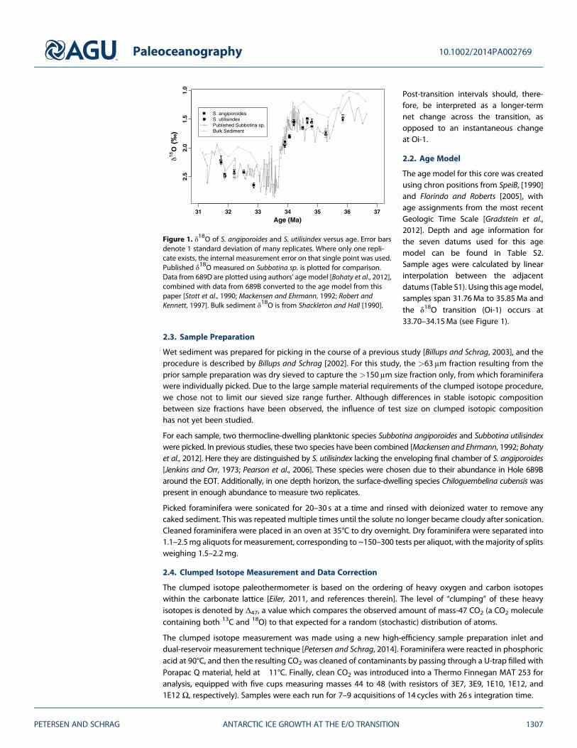
The age model for this core was createdusing chron positions from SpeiB, [1990]and Florindo and Roberts [2005], withage assignments from the most recentGeologic Time Scale [Gradstein et al.,2012]. Depth and age information forthe seven datums used for this agemodel can be found in Table S2.Sample ages were calculated by linearinterpolation between the adjacentdatums (Table S1). Using this agemodel,samples span 31.76Ma to 35.85Ma andthe δ18O transition (Oi-1) occurs at33.70–34.15Ma (see Figure 1).

2.3. Sample Preparation

Wet sediment was prepared for picking in the course of a previous study [Billups and Schrag, 2003], and theprocedure is described by Billups and Schrag [2002]. For this study, the >63μm fraction resulting from theprior sample preparation was dry sieved to capture the >150μm size fraction only, from which foraminiferawere individually picked. Due to the large sample material requirements of the clumped isotope procedure,we chose not to limit our sieved size range further. Although differences in stable isotopic compositionbetween size fractions have been observed, the influence of test size on clumped isotopic compositionhas not yet been studied.

For each sample, two thermocline-dwelling planktonic species Subbotina angiporoides and Subbotina utilisindexwere picked. In previous studies, these two species have been combined [Mackensen and Ehrmann, 1992; Bohatyet al., 2012]. Here they are distinguished by S. utilisindex lacking the enveloping final chamber of S. angiporoides[Jenkins and Orr, 1973; Pearson et al., 2006]. These species were chosen due to their abundance in Hole 689Baround the EOT. Additionally, in one depth horizon, the surface-dwelling species Chiloguembelina cubensis waspresent in enough abundance to measure two replicates.

Picked foraminifera were sonicated for 20–30 s at a time and rinsed with deionized water to remove anycaked sediment. This was repeated multiple times until the solute no longer became cloudy after sonication.Cleaned foraminifera were placed in an oven at 35°C to dry overnight. Dry foraminifera were separated into1.1–2.5mg aliquots for measurement, corresponding to ~150–300 tests per aliquot, with themajority of splitsweighing 1.5–2.2mg.

2.4. Clumped Isotope Measurement and Data Correction

The clumped isotope paleothermometer is based on the ordering of heavy oxygen and carbon isotopeswithin the carbonate lattice [Eiler, 2011, and references therein]. The level of “clumping” of these heavyisotopes is denoted by Δ47, a value which compares the observed amount of mass-47 CO2 (a CO2 moleculecontaining both 13C and 18O) to that expected for a random (stochastic) distribution of atoms.

The clumped isotope measurement was made using a new high-efficiency sample preparation inlet anddual-reservoir measurement technique [Petersen and Schrag, 2014]. Foraminifera were reacted in phosphoricacid at 90°C, and then the resulting CO2 was cleaned of contaminants by passing through a U-trap filled withPorapac Q material, held at �11°C. Finally, clean CO2 was introduced into a Thermo Finnegan MAT 253 foranalysis, equipped with five cups measuring masses 44 to 48 (with resistors of 3E7, 3E9, 1E10, 1E12, and1E12 Ω, respectively). Samples were each run for 7–9 acquisitions of 14 cycles with 26 s integration time.

31 32 33 34 35 36 37

2.5

2.0

1.5

1.0

Age (Ma)

18O

()

S. angiporoidesS. utilisindexPublished Subbotina sp.Bulk Sediment

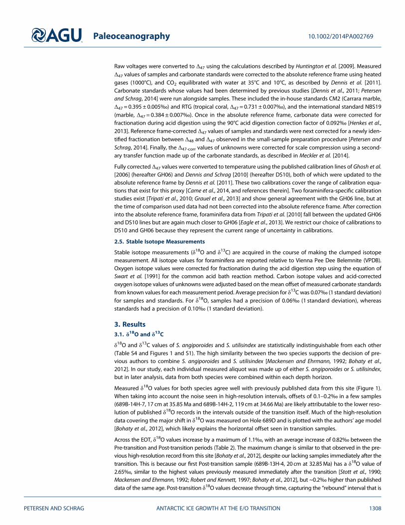
Figure 1. δ18O of S. angiporoides and S. utilisindex versus age. Error barsdenote 1 standard deviation of many replicates. Where only one repli-cate exists, the internal measurement error on that single point was used.Published δ18O measured on Subbotina sp. is plotted for comparison.Data from 689D are plotted using authors’ age model [Bohaty et al., 2012],combined with data from 689B converted to the age model from thispaper [Stott et al., 1990; Mackensen and Ehrmann, 1992; Robert andKennett, 1997]. Bulk sediment δ18O is from Shackleton and Hall [1990].

Paleoceanography 10.1002/2014PA002769

PETERSEN AND SCHRAG ANTARCTIC ICE GROWTH AT THE E/O TRANSITION 1307

Raw voltages were converted to Δ47 using the calculations described by Huntington et al. [2009]. MeasuredΔ47 values of samples and carbonate standards were corrected to the absolute reference frame using heatedgases (1000°C), and CO2 equilibrated with water at 35°C and 10°C, as described by Dennis et al. [2011].Carbonate standards whose values had been determined by previous studies [Dennis et al., 2011; Petersenand Schrag, 2014] were run alongside samples. These included the in-house standards CM2 (Carrara marble,Δ47 = 0.395 ± 0.005‰) and RTG (tropical coral, Δ47 = 0.731 ± 0.007‰), and the international standard NBS19(marble, Δ47 = 0.384 ± 0.007‰). Once in the absolute reference frame, carbonate data were corrected forfractionation during acid digestion using the 90°C acid digestion correction factor of 0.092‰ [Henkes et al.,2013]. Reference frame-corrected Δ47 values of samples and standards were next corrected for a newly iden-tified fractionation between Δ48 and Δ47 observed in the small-sample preparation procedure [Petersen andSchrag, 2014]. Finally, the Δ47-corr values of unknowns were corrected for scale compression using a second-ary transfer function made up of the carbonate standards, as described in Meckler et al. [2014].

Fully corrected Δ47 values were converted to temperature using the published calibration lines of Ghosh et al.[2006] (hereafter GH06) and Dennis and Schrag [2010] (hereafter DS10), both of which were updated to theabsolute reference frame by Dennis et al. [2011]. These two calibrations cover the range of calibration equa-tions that exist for this proxy [Came et al., 2014, and references therein]. Two foraminifera-specific calibrationstudies exist [Tripati et al., 2010; Grauel et al., 2013] and show general agreement with the GH06 line, but atthe time of comparison used data had not been corrected into the absolute reference frame. After correctioninto the absolute reference frame, foraminifera data from Tripati et al. [2010] fall between the updated GH06and DS10 lines but are again much closer to GH06 [Eagle et al., 2013]. We restrict our choice of calibrations toDS10 and GH06 because they represent the current range of uncertainty in calibrations.

2.5. Stable Isotope Measurements

Stable isotope measurements (δ18O and δ13C) are acquired in the course of making the clumped isotopemeasurement. All isotope values for foraminifera are reported relative to Vienna Pee Dee Belemnite (VPDB).Oxygen isotope values were corrected for fractionation during the acid digestion step using the equation ofSwart et al. [1991] for the common acid bath reaction method. Carbon isotope values and acid-correctedoxygen isotope values of unknowns were adjusted based on themean offset of measured carbonate standardsfrom known values for eachmeasurement period. Average precision for δ13C was 0.07‰ (1 standard deviation)for samples and standards. For δ18O, samples had a precision of 0.06‰ (1 standard deviation), whereasstandards had a precision of 0.10‰ (1 standard deviation).

3. Results3.1. δ18O and δ13C

δ18O and δ13C values of S. angiporoides and S. utilisindex are statistically indistinguishable from each other(Table S4 and Figures 1 and S1). The high similarity between the two species supports the decision of pre-vious authors to combine S. angiporoides and S. utilisindex [Mackensen and Ehrmann, 1992; Bohaty et al.,2012]. In our study, each individual measured aliquot was made up of either S. angiporoides or S. utilisindex,but in later analysis, data from both species were combined within each depth horizon.

Measured δ18O values for both species agree well with previously published data from this site (Figure 1).When taking into account the noise seen in high-resolution intervals, offsets of 0.1–0.2‰ in a few samples(689B-14H-7, 17 cm at 35.85Ma and 689B-14H-2, 119 cm at 34.66Ma) are likely attributable to the lower reso-lution of published δ18O records in the intervals outside of the transition itself. Much of the high-resolutiondata covering the major shift in δ18O was measured on Hole 689D and is plotted with the authors’ age model[Bohaty et al., 2012], which likely explains the horizontal offset seen in transition samples.

Across the EOT, δ18O values increase by a maximum of 1.1‰, with an average increase of 0.82‰ between thePre-transition and Post-transition periods (Table 2). The maximum change is similar to that observed in the pre-vious high-resolution record from this site [Bohaty et al., 2012], despite our lacking samples immediately after thetransition. This is because our first Post-transition sample (689B-13H-4, 20 cm at 32.85Ma) has a δ18O value of2.65‰, similar to the highest values previously measured immediately after the transition [Stott et al., 1990;Mackensen and Ehrmann, 1992; Robert and Kennett, 1997; Bohaty et al., 2012], but ~0.2‰ higher than publisheddata of the same age. Post-transition δ18O values decrease through time, capturing the “rebound” interval that is

Paleoceanography 10.1002/2014PA002769

PETERSEN AND SCHRAG ANTARCTIC ICE GROWTH AT THE E/O TRANSITION 1308

also visible in the published data from this site [Mackensen and Ehrmann, 1992; Robert and Kennett, 1997; Bohatyet al., 2012] and in the global benthic stack [Zachos et al., 2001; Cramer et al., 2009].

δ13C values gradually decrease from 1.5‰ to 1.1‰ toward the present, in general agreement with previouslypublished studies [Mackensen and Ehrmann, 1992;Mead and Hodell, 1995; Robert and Kennett, 1997] (Figure S1).Transition samples are lower than published data, as is sample 689B-14H-3, 20 cm (34.81Ma). However, onlylow-resolution δ13C records exist for this site, which could explain these offsets. For both δ18O and δ13C, stableisotope data from S. angiporoides and S. utilisindex differ substantially from bulk sediment stable isotope values(Figures 1 and S1) [Shackleton and Hall, 1990], suggesting our cleaning procedures were sufficient to removeany sediment attached to foraminifera tests.

In one sample (689B-14H-2, 67 cm, at 34.50Ma), two replicates of Chiloguembelina cubensis were measured,giving δ13C and δ18O values of 1.998 ± 0.018‰ and 1.569 ± 0.040‰. This compares well with twomeasurements of this species at 122.06 and 122.8mbsf that average to 2.10 ± 0.17‰ and 1.69 ± 0.07‰[Stott et al., 1990]. At the same depth horizon, we measure δ13C and δ18O values of 1.429 ± 0.047‰ and1.651 ± 0.028‰ for the combined Subbotina species.

3.2. Δ47 and Temperature

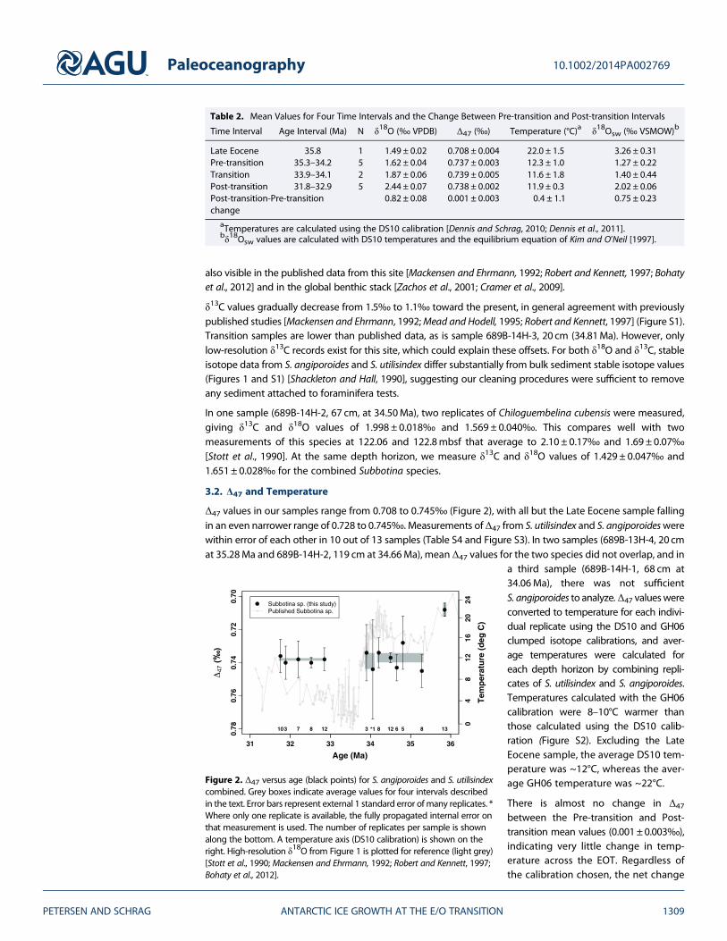
Δ47 values in our samples range from 0.708 to 0.745‰ (Figure 2), with all but the Late Eocene sample fallingin an even narrower range of 0.728 to 0.745‰. Measurements ofΔ47 from S. utilisindex and S. angiporoideswerewithin error of each other in 10 out of 13 samples (Table S4 and Figure S3). In two samples (689B-13H-4, 20 cmat 35.28Ma and 689B-14H-2, 119 cm at 34.66Ma), mean Δ47 values for the two species did not overlap, and in

a third sample (689B-14H-1, 68 cm at34.06Ma), there was not sufficientS. angiporoides to analyze.Δ47 valueswereconverted to temperature for each indivi-dual replicate using the DS10 and GH06clumped isotope calibrations, and aver-age temperatures were calculated foreach depth horizon by combining repli-cates of S. utilisindex and S. angiporoides.Temperatures calculated with the GH06calibration were 8–10°C warmer thanthose calculated using the DS10 calib-ration (Figure S2). Excluding the LateEocene sample, the average DS10 tem-perature was ~12°C, whereas the aver-age GH06 temperature was ~22°C.

There is almost no change in Δ47

between the Pre-transition and Post-transition mean values (0.001±0.003‰),indicating very little change in temp-erature across the EOT. Regardless ofthe calibration chosen, the net change

Table 2. Mean Values for Four Time Intervals and the Change Between Pre-transition and Post-transition Intervals

Time Interval Age Interval (Ma) N δ18O (‰ VPDB) Δ47 (‰) Temperature (°C)a δ18Osw (‰ VSMOW)b

Late Eocene 35.8 1 1.49 ± 0.02 0.708 ± 0.004 22.0 ± 1.5 3.26 ± 0.31Pre-transition 35.3–34.2 5 1.62 ± 0.04 0.737 ± 0.003 12.3 ± 1.0 1.27 ± 0.22Transition 33.9–34.1 2 1.87 ± 0.06 0.739 ± 0.005 11.6 ± 1.8 1.40 ± 0.44Post-transition 31.8–32.9 5 2.44 ± 0.07 0.738 ± 0.002 11.9 ± 0.3 2.02 ± 0.06Post-transition-Pre-transitionchange

0.82 ± 0.08 0.001 ± 0.003 �0.4 ± 1.1 0.75 ± 0.23

aTemperatures are calculated using the DS10 calibration [Dennis and Schrag, 2010; Dennis et al., 2011].bδ18Osw values are calculated with DS10 temperatures and the equilibrium equation of Kim and O’Neil [1997].

Age (Ma)

47 (

)

31 32 33 34 35 36

0.78

0.76

0.74

0.72

0.70

04

812

1620

24

Tem

per

atu

re (

deg

C)

Figure 2. Δ47 versus age (black points) for S. angiporoides and S. utilisindexcombined. Grey boxes indicate average values for four intervals describedin the text. Error bars represent external 1 standard error of many replicates. *Where only one replicate is available, the fully propagated internal error onthat measurement is used. The number of replicates per sample is shownalong the bottom. A temperature axis (DS10 calibration) is shown on theright. High-resolution δ18O from Figure 1 is plotted for reference (light grey)[Stott et al., 1990; Mackensen and Ehrmann, 1992; Robert and Kennett, 1997;Bohaty et al., 2012].

Paleoceanography 10.1002/2014PA002769

PETERSEN AND SCHRAG ANTARCTIC ICE GROWTH AT THE E/O TRANSITION 1309

in temperature between Pre-transitionand Post-transition periods is thesame, within error (GH06=�0.4± 0.7°C,DS10 =�0.4 ± 1.1°C). In both cases,the data show a small cooling acrossthe EOT.

The Late Eocene sample (689B-14H-7,17 cm, at 35.85Ma) has a Δ47 value of0.708‰, outside the range of the othersamples, suggesting warmer tempera-tures in the latest Eocene. This convertsto a temperature of 22.0 ± 1.5°C usingthe DS10 calibration or 27.6 ± 0.9°Cusing GH06. In both calibrations, thissample indicates much warmer condi-tions at 35.8Ma than in the Pre-transitionand Post-transition intervals. This 5–10°Cdifference is not mirrored in δ18O

values, which are only 0.2‰ lower in the late Eocene than in the Pre-transition interval. The late Eocenevalue is made up of 13 analyses, made over two measurement periods. Despite being picked and cleanedat different times and corrected using different standard gases and carbonates, the mean values from thetwo measurement periods (n= 6 and n= 7) differ by 0.007 ± 0.009‰, within error of zero, suggesting thatthis is not a measurement artifact.

Comparison of the temperatures calculated using the two different calibrations with other proxies showsmuch better agreement with the DS10 temperatures (see section 4). This, combined with the fact that theDS10 calibration was performed in the same lab as this study using very similar procedures, lends credenceto the DS10 temperatures over the GH06 temperatures in this case. For further calculations and discussion,we use the DS10 temperatures unless otherwise indicated.

In the one sample where C. cubensis was abundant enough for analysis (689B-14H-2, 67 cm), the two mea-sured replicates recorded very disparate Δ47 values, resulting in a mean value with a very large error(0.699 ± 0.030‰). This is equivalent to a DS10 temperature of 25.7 ± 11.0°C. With an error so large, it is notpossible to conclude anything about the environment of C. cubensis relative to the Subbotina species or tolook at temperature gradients with depth.

3.3. δ18Osw and Ice Volume Estimates

Although δ18O values change dramatically, both through the transition and within the rebound interval, Δ47

values remain nearly constant, requiring that the large change in foraminiferal δ18O be accommodated com-pletely by changes in the isotopic composition of seawater (δ18Osw). δ

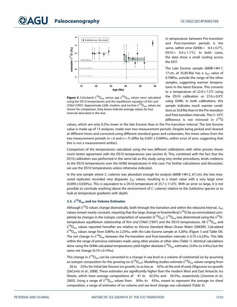
18Osw was determined using the δ18O-temperature equilibrium relationship of Kim and O’Neil [1997] and the DS10 temperatures. All δ18Osw andδ18Oice values reported hereafter are relative to Vienna Standard Mean Ocean Water (SMOW). Calculatedδ18Osw values range from 0.80‰ to 2.25‰, with the Late Eocene sample at 3.26‰ (Figure 3 and Table S4).The net change in δ18Osw between the Pre-transition and Post-transition intervals is 0.75± 0.23‰. This fallswithin the range of previous estimates made using other proxies at other sites (Table 1). Identical calculationsdone using the GH06-calculated temperatures yield higher absolute δ18Osw estimates (3.0‰ to 4.4‰) but thesame net change (0.74± 0.14‰).

This change in δ18Osw can be converted to a change in sea level or a volume of continental ice by assumingan isotopic composition for the growing ice (δ18Oice). Modeling studies estimate δ18Oice values ranging from�20 to�25‰ for initial late Eocene ice growth, to as low as�42‰ at the end of early Oligocene ice growth[DeConto et al., 2008]. These estimates are significantly higher than the modern West and East Antarctic IceSheets, which have average compositions of �41 to �42.5‰ and �56.5‰, respectively [Lhomme et al.,2005]. Using a range of δ18Oice values from �30‰ to �45‰, meant to represent the average ice sheetcomposition, a range of estimates of ice volume and sea level change was calculated (Table 3).

31 32 33 34 35 36

-10

12

34

Age (Ma)

Figure 3. Calculated δ18Osw versus age δ18Osw values were calculatedusing the DS10 temperatures and the equilibrium equation of Kim andO’Neil [1997]. Approximate LGM, modern, and ice-free δ18Osw values areshown for comparison. Grey boxes indicate average values for fourintervals described in the text.

Paleoceanography 10.1002/2014PA002769

PETERSEN AND SCHRAG ANTARCTIC ICE GROWTH AT THE E/O TRANSITION 1310

Using an intermediate value for δ18Oice (�35 to �40‰) and a change in δ18Osw of 0.75‰, we estimate2.9–3.3 × 107 km3 of ice growth, equivalent to 107–122% of the modern Antarctic ice sheet (AIS) volume(Table 3). This estimate is higher but consistent with modeling studies that have sustained ice sheets onthe order of 2.1 × 107 km3 on Antarctica under Eocene-Oligocene conditions [DeConto et al., 2008]. At theEOT, the land area of Antarctica was 10–20% larger than today, which, based on the curvature of a grow-ing ice sheet, would scale to an even greater increase in potential ice volume that could be housed on thecontinent [Wilson and Luyendyk, 2009]. In addition, any ice that was growing in the Northern Hemisphereor elsewhere at high elevation would reduce the volume that would need to be accommodated on theAntarctic continent.

The ice volume calculated from the intermediate δ18Oice composition may be converted into a eustatic sealevel change by assuming a fixed ocean area (Table 3). Our estimate of 79–91m eustatic sea level fallrepresents the long-term storage of ice on Antarctica 1–2Myr after the EOT and is not directly comparableto other estimates of sea level change occurring at Oi-1. Nevertheless, our estimate is consistent withsedimentological evidence of 80 ± 25m of eustatic sea level fall across the whole EOT [Miller et al., 2009,and references therein].

4. Discussion4.1. Comparison to Temperature Estimates From Other Proxies

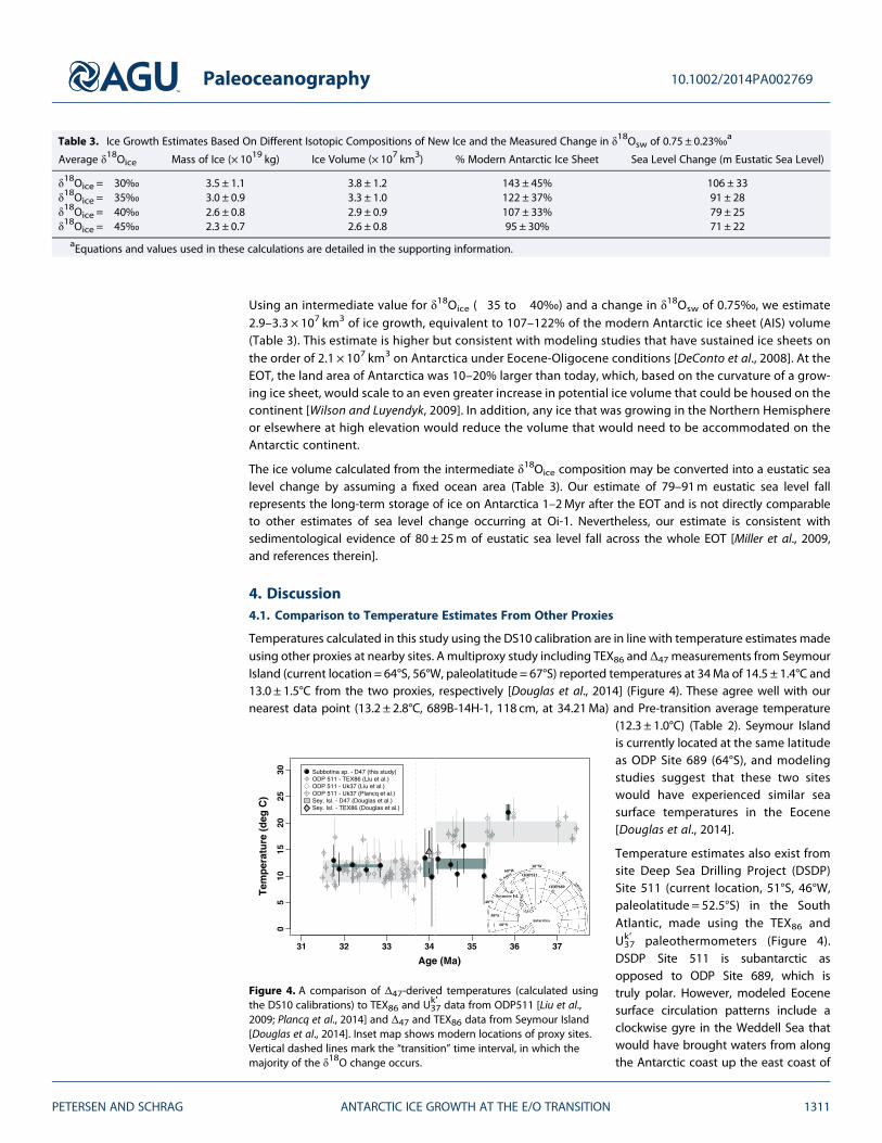
Temperatures calculated in this study using the DS10 calibration are in line with temperature estimates madeusing other proxies at nearby sites. A multiproxy study including TEX86 and Δ47 measurements from SeymourIsland (current location = 64°S, 56°W, paleolatitude= 67°S) reported temperatures at 34Ma of 14.5 ± 1.4°C and13.0 ± 1.5°C from the two proxies, respectively [Douglas et al., 2014] (Figure 4). These agree well with ournearest data point (13.2 ± 2.8°C, 689B-14H-1, 118 cm, at 34.21Ma) and Pre-transition average temperature

(12.3 ± 1.0°C) (Table 2). Seymour Islandis currently located at the same latitudeas ODP Site 689 (64°S), and modelingstudies suggest that these two siteswould have experienced similar seasurface temperatures in the Eocene[Douglas et al., 2014].

Temperature estimates also exist fromsite Deep Sea Drilling Project (DSDP)Site 511 (current location, 51°S, 46°W,paleolatitude = 52.5°S) in the SouthAtlantic, made using the TEX86 andUk′37 paleothermometers (Figure 4).

DSDP Site 511 is subantarctic asopposed to ODP Site 689, which istruly polar. However, modeled Eocenesurface circulation patterns include aclockwise gyre in the Weddell Sea thatwould have brought waters from alongthe Antarctic coast up the east coast of

Table 3. Ice Growth Estimates Based On Different Isotopic Compositions of New Ice and the Measured Change in δ18Osw of 0.75 ± 0.23‰a

Average δ18Oice Mass of Ice (× 1019 kg) Ice Volume (× 107 km3) % Modern Antarctic Ice Sheet Sea Level Change (m Eustatic Sea Level)

δ18Oice =�30‰ 3.5 ± 1.1 3.8 ± 1.2 143 ± 45% 106 ± 33δ18Oice =�35‰ 3.0 ± 0.9 3.3 ± 1.0 122 ± 37% 91 ± 28δ18Oice =�40‰ 2.6 ± 0.8 2.9 ± 0.9 107 ± 33% 79 ± 25δ18Oice =�45‰ 2.3 ± 0.7 2.6 ± 0.8 95 ± 30% 71 ± 22

aEquations and values used in these calculations are detailed in the supporting information.

Figure 4. A comparison of Δ47-derived temperatures (calculated usingthe DS10 calibrations) to TEX86 and Uk′37 data from ODP511 [Liu et al.,2009; Plancq et al., 2014] and Δ47 and TEX86 data from Seymour Island[Douglas et al., 2014]. Inset map shows modern locations of proxy sites.Vertical dashed lines mark the “transition” time interval, in which themajority of the δ18O change occurs.

Paleoceanography 10.1002/2014PA002769

PETERSEN AND SCHRAG ANTARCTIC ICE GROWTH AT THE E/O TRANSITION 1311

South America [Douglas et al., 2014], potentially giving these two sites more similar temperatures than theirlatitudinal positions would suggest. The Pre-transition average temperature at DSDP Site 511 is 18.3±2.0°C,covering the age range of 34.15–37.15Ma [Liu et al., 2009; Plancq et al., 2014]. This is 6°C warmer thanour Pre-transition average (12.3 ± 1.0°C, 34.2–35.3 Ma) but represents a period that extends further intothe Eocene. In contrast, our Late Eocene sample (22.0 ± 1.5°C) is warmer than the DSDP Site 511 Pre-transitionaverage but is within error of the two closest points (21.4 ± 1.9°C, 35.98Ma) [Liu et al., 2009] and theaverage for an earlier interval (19.2 ± 0.5°C, 35.28–37.15Ma) [Liu et al., 2009; Plancq et al., 2014]. ThePost-transition average for DSDP Site 511 is 10.9± 2.1°C (31.5–33.7Ma) [Liu et al., 2009; Plancq et al., 2014],in agreement with our Post-transition average (11.9 ± 0.3°C, 31.8–32.9Ma).

Three proxies (Δ47, TEX86, and Uk′37) now suggest subantarctic and Antarctic temperatures of 10–12°C in the

early Oligocene [Liu et al., 2009; Douglas et al., 2014; Plancq et al., 2014] (this study). In high northern lati-tudes, similarly warm temperatures existed. In the Norwegian Sea (ODP Site 913, 75°N), TEX86, methylationand cyclization of branched tetraethers (MBT index, CBT ratio), and pollen reconstructions record tempera-tures of 8–10°C, 10 ± 3°C, and 11 ± 2°C, respectively, for the early Oligocene [Schouten et al., 2008]. Thesetemperatures may seem too warm, considering the many studies that now indicate a substantial Antarcticice sheet at this time (Table 1). However, these high-latitude proxy reconstructions may be biased toward sum-mertime temperatures due to light limitation during polar night [Eldrett et al., 2009]. For comparison, a model-ing study found austral summertime (December-January-February) temperatures of ~4–7°C for 65°S with2.5 × PAL CO2 (700 ppm) and a full ice sheet on Antarctica, or ~7–11°C with no ice sheet [Pollard andDeConto, 2005].

4.2. Lack of Temperature Change at ODP Site 689

Most other studies of the Eocene-Oligocene transition record some amount of surface or deep cooling(2–5°C) across the transition, which is needed to account for the large magnitude change in δ18O(>1.2‰) without requiring excessive ice growth. In contrast, the measurements on thermocline-dwelling S. angiporoides and S. utilisindex shown here record less than half a degree of cooling betweenPre-transition and Post-transition intervals. Due to the spacing of samples around the EOT in this study,our calculated change in temperature represents a longer-term net change and does not capture anyinstantaneous changes across the transition. A larger cooling may have occurred during Oi-1 but wouldhave to have mostly reversed by 32.85Ma to be consistent with our first Post-transition sample. Thisreversal is seen in Mg/Ca data from the Kerguelan Plateau, which indicate a more pronounced coolingin the earliest Oligocene that reversed by 33Ma, and in Mg/Ca data from ODP Site 689, which show asmaller syn-transition cooling that is reversed by 33.5 Ma (although this record ends before our firstPost-transition sample, so direct comparison is impossible) [Bohaty et al., 2012]. Our estimate of long-termtemperature change (�0.4±1.1°C) allows for up to 1.5°C of cooling within error, which is compatible with otherstudies. This suggests that the long-term shift in δ18O across the EOT was mainly the result of a semipermanentshift in continental ice volume, as opposed to significant cooling.

It is also possible that ocean waters did cool at this site, but that these thermocline-dwelling species did notrecord the cooling. The thermocline temperature could have remained the same, while the surface and/ordeep water cooled, resulting in a shallower temperature gradient with depth. Alternatively, with or withouta change in thermocline structure, S. angiporoides and S. utilisindex could have changed their depth habitatslightly to maintain the same thermal environment while ocean temperatures cooled. Such an adjustmentwould have been easier for these species than for surface-dwelling or benthic foraminifera due to the largethermal gradient found in the thermocline, requiring a much smaller change in depth (and therefore lightconditions) to maintain the same temperature.

Regardless of whether the thermal gradient changed or these species adjusted their depth habitat to main-tain the same thermal conditions, no change in temperature was recorded between the Pre-transition andPost-transition intervals. Therefore, assuming the ice volume signal was well mixed in the oceans, changesin δ18O recorded in this study indicate global changes in δ18Osw.

4.3. Extremely High δ18Osw Values

Despite the agreement between DS10-calculated temperatures and temperature estimates from otherproxies at nearby sites, the δ18Osw values calculated using the DS10 temperatures are unreasonably high.

Paleoceanography 10.1002/2014PA002769

PETERSEN AND SCHRAG ANTARCTIC ICE GROWTH AT THE E/O TRANSITION 1312

In the late Eocene, δ18Osw values are expected to be between �1 and 0‰, indicating the existence ofonly small, transient continental ice growth prior to the major ice growth event at the EOT [Browninget al., 1996; Sagnotti et al., 1998; Tripati et al., 2005]. This is nearly 2‰ lower than δ18Osw values calculatedin this study. δ18Osw values of around +1‰ prior to the EOT ice growth require ice volumes in excess of theLast Glacial Maximum (LGM), when ice sheets covered large parts of North America. Unlike at the LGM, it isthought that in the Eocene, Northern Hemisphere ice was restricted to mountain glaciers only [Edgar et al.,2007; Eldrett et al., 2009], which is not sufficient to explain such high δ18Osw values. This discrepancybetween calculated and expected δ18Osw values may be due to (1) errors in the absolute Δ47-T calibration,producing temperatures that are too warm, (2) vital effects in these extinct species of foraminifera,resulting in δ18O values enriched relative to equilibrium with seawater, or (3) diagenesis causing lowerΔ47 and/or higher δ

18O.

Differences in the Δ47-T calibration would influence absolute temperature (and δ18Osw) values but wouldhave no impact on the calculated change in temperature, which would be near-zero regardless of the choiceof calibration (as demonstrated by the equivalent change in temperature calculated by the GH06 and DS10calibrations). The many published Δ47-T calibrations tend to fall into two groups, those with steeper slopessimilar to GH06 and those with shallower slopes similar to DS10 [Came et al., 2014, and references therein;Tang et al., 2014, and references therein]. Among the calibrations with the shallower DS10 slope, the interceptvalues differ by ~0.02–0.04‰ in the Δ47 range of interest [Schauble et al., 2006; Dennis and Schrag, 2010;Henkes et al., 2013; Hill et al., 2014; Eagle et al., 2013]. A decrease of 0.02‰ in the intercept of the calibrationwould result in a decrease of ~6°C for the mean temperature both before and after the transition (from ~12 to~6°C in both periods). At these lower temperatures, δ18Osw values become �0.12‰ before the EOT and0.63‰ after, showing the same magnitude of change (0.75‰), but absolute values much closer to thoseexpected for a nearly ice-free Eocene. In order to get a Pre-transition δ18Osw value equal to the ice-free oceanend-member, the intercept would need to decrease by 0.031‰. However, at this point the calculatedtemperatures are 2–3°C, much lower than temperature estimates from other nearby proxies. Choice of theDS10 calibration over the other shallow slope calibrations with different intercepts is supported by the factthat the DS10 calibration was performed in the same lab as this study, eliminating the potentially biasinginfluence of any interlab differences in procedure.

Alternatively, the high δ18Osw values may be due to vital effects in S. angiporoides and S. utilisindex affectingδ18O. Subbotina species, including S. angiporoides and S. utilisindex, their ancestor Subbotina linaperta[Pearson et al., 2006], and others, often, but not always, record higher δ18O (and lower δ13C) values than otherplanktonic foraminifera, resulting in their designation as thermocline dwellers [Poore and Matthews, 1984;Keigwin and Corliss, 1986; Sexton et al., 2006;Wade and Pearson, 2008]. For example, the size of the observedoffset in δ18O between Subbotina sp. and Chiloguembelina cubensis (the planktonic species often recordingthe lowest values) ranges from 0‰ up to 1.75‰ [Poore and Matthews, 1984; Keigwin and Corliss, 1986]. Itis possible that instead of living in the cooler thermocline, Subbotina sp. were surface dwellers that incorpo-rated more 18O into their shells than would be expected from equilibrium with seawater (i.e., a vital effect),resulting in higher δ18O and warm (surface) Δ47 temperatures. Such vital effects would have to increaseδ18O on the order of 1.5‰ above equilibrium to get reasonable δ18Osw values, given the temperatures mea-sured in this study. Further work comparing clumped isotope temperatures of different species with theassumed habitats from δ18O depth ranking could resolve these questions and strengthen paleoclimate inter-pretations. Typically, vital effects in foraminifera are expressed as a fixed offset from equilibrium values (e.g.,+0.64‰ for Cibicidoides sp.) so would therefore only affect the absolute δ18O and δ18Osw values but not therelative change in either across the EOT. There is no evidence for vital effects in Δ47 for foraminifera [Tripatiet al., 2010].

Finally, the high δ18Osw values could be caused by diagenetic effects that increased either temperature or δ18Ovalues. Minimal resetting of δ18O values is expected in high-latitude sites such as ODP 689 frommodeling of sedi-ment burial and pore water chemistry [Schrag et al., 1995]. Additional early precipitation of calcite in the colderenvironment of the seafloor or surface sediments would increase δ18O but decrease Δ47 temperatures, resultingin little change in δ18Osw. The samples in this study were taken from 110 to 130mbsf and experienced tempera-tures of only ~6–13°C at these depths, according to limited downhole temperature data at ODP Sites 689 and 690[Nagao, 1990]. Resetting of the clumped isotope signal by solid-state bond reordering only occurs at temperatures

Paleoceanography 10.1002/2014PA002769

PETERSEN AND SCHRAG ANTARCTIC ICE GROWTH AT THE E/O TRANSITION 1313

above 100–150°C [Henkes et al., 2014], much higher than those experienced by these samples. Recrystallizationdeep in the sediment column at temperatures of 6–13°C could possibly explain our Pre-transition andPost-transition data but cannot explain the late Eocene sample, which is 22°C.

4.4. Influence of Changing Carbonate Ion Concentrations on Ice Volume Estimates

Across the EOT, seawater carbonate ion concentration ([CO32�]) has been calculated to change on the order

of 36μmol/kg in the deep Pacific [Lear et al., 2010] to 19–29μmol/kg in the South Atlantic [Lear et al., 2010;Peck et al., 2010] from paired Li/Ca and Mg/Ca measurements. These values agree with a change in [CO3

2�] of19μmol/kg calculated for a 1.2 km deepening of the carbonate compensation depth [Lear et al., 2010;Broecker and Peng, 1982]. It has been shown that increases in [CO3

2�] cause reduced stable isotope valuesin planktonic foraminifera and other single-celled planktonic organisms with a slope of �0.0022‰ δ18O/(μmol/kg [CO3

2�]) for Orbulina universa [Spero et al., 1997], �0.0048 for a coccolithophore species, and�0.0243 for a calcareous dinoflagellate [Ziveri et al., 2012]. Based on the above estimates of changes in[CO3

2�], this could influence δ18O values by 0.04–0.08‰ for foraminifera, diminishing the full magnitudeof the EOT signal. If instead the larger slope for coccolithophores was used, δ18O values could be diminishedby 0.09–0.17‰ across the transition. This influence would differ from site to site, basin to basin, and espe-cially with depth of the core. A site like ODP Site 1218, which was near the CCD prior to the EOT [Coxallet al., 2005], likely experienced a larger change in [CO3

2�] (36μmol/kg) [Lear et al., 2010], whereas a shallowersite may have seen a smaller impact. These site-to-site and depth-dependent differences may explain someof the range in ice volume estimates shown in Table 1, because the calculated changes in δ18Osw may be vari-ably muted according to the local change in [CO3

2�].

5. Conclusions

Clumped isotope measurements on Southern Ocean thermocline-dwelling foraminifera record a minorchange in temperature (�0.4 ± 1.1°C) across the Eocene-Oligocene transition. Mean temperatures at siteODP Site 689 were 12.3°C before and 11.9°C after the transition, in line with temperature estimates fromnearby sites [Douglas et al., 2014; Liu et al., 2009; Plancq et al., 2014]. These temperatures represent averageconditions in the 0–1.5Myr before and 1–2Myr after the main Oi-1 transition and may not capture the fullchange in temperature that occurred at the EOT. When combined with the change in δ18O, this coolingequates to a change in δ18Osw of 0.75 ± 0.23‰ between these intervals, equivalent to an ice volume increaseof 2.9–3.3 × 107 km3, or roughly 110–120% of the modern Antarctic ice sheet volume. These values are withinthe range of previous estimates (Table 2). The absolute values of δ18Osw are 1–2‰ higher than expected forthis time period, which may be due to uncertainty in the Δ47-T calibration and/or vital effects occurring inthese species of foraminifera. Despite high absolute values, the calculated difference in δ18Osw is robustand is within the range of previous estimates. Overall, these results indicate that the longer-term shift inδ18O across the EOT is due predominantly to a semipermanent shift in continental ice volume, and thatany net temperature changes were less than ~1.5°C at this site. This result is not at odds with previous studiesthat measured greater cooling at the EOT. Larger instantaneous cooling could have occurred during the tran-sition itself (not captured in this study) but must have mostly reversed by 32.75Ma.

ReferencesBillups, K., and D. P. Schrag (2002), Paleotemperatures and ice volume of the past 27 Myr revisited with paired Mg/Ca and

18O/

16O

measurements on benthic foraminifera, Paleoceanography, 17(1), 3-1–3-11, doi:10.1029/2000PA000567.Billups, K., and D. P. Schrag (2003), Application of benthic foraminiferal Mg/Ca to questions of Cenozoic climate change, Earth Planet. Sci. Lett.,

209(1–2), 181–195, doi:10.1016/S0012-821X(03)00067-0.Bohaty, S. M., J. C. Zachos, and M. L. Delaney (2012), Foraminiferal Mg/Ca evidence for Southern Ocean cooling across the Eocene-Oligocene

transition, Earth Planet. Sci. Lett., 317–318, 251–261, doi:10.1016/j.epsl.2011.11.037.Broecker, W. S., and T.-H. Peng (1982), Tracers in the Sea, 169 pp., Lamont-Doherty Geological Observatory of Columbia Univ., Palisades,

New York.Browning, J. V., K. G. Miller, and D. K. Pak (1996), Global implications of lower to middle Eocene sequence boundaries on the New Jersey

coastal plain: The icehouse cometh, Geology, 24(7), 639–642, doi:10.1130/0091-7613(1996)024<0639:GIOLTM>2.3.CO;2.Came, R. E., U. Brand, and H. P. Affek (2014), Clumped isotope signatures in modern brachiopod carbonate, Chem. Geol., 377, 20–30,

doi:10.1016/j.chemgeo.2014.04.004.Coxall, H. K., P. A. Wilson, H. Pälike, C. H. Lear, and J. Backman (2005), Rapid stepwise onset of Antarctic glaciation and deeper calcite com-

pensation in the Pacific Ocean, Nature, 433, 53–57, doi:10.1038/nature03135.Cramer, B. S., J. R. Toggweiler, J. D. Wright, M. E. Katz, and K. G. Miller (2009), Ocean overturning since the Late Cretaceous: Inferences from a

new benthic foraminiferal isotope compilation, Paleoceanography, 24, PA4216, doi:10.1029/2008PA001683.

Paleoceanography 10.1002/2014PA002769

PETERSEN AND SCHRAG ANTARCTIC ICE GROWTH AT THE E/O TRANSITION 1314

AcknowledgmentsThe data collected in this study areavailable in the supporting information.This work was supported by Henry andWendy Breck and by the HarvardUniversity GSAS Merit Fellowship. Theauthors would like to thank G. Eischeid,S. Manley, J. Shakun, and F. Chen forlaboratory assistance. We would alsolike to thank two reviewers for theirhelpful comments.

Cramer, B. S., K. G. Miller, P. J. Barrett, and J. D. Wright (2011), Late Cretaceous-Neogene trends in deep ocean temperature and continentalice volume: Reconciling records of benthic foraminiferal geochemistry (δ

18Oand Mg/Ca) with sea level history, J. Geophys. Res., 116,

C12023, doi:10.1029/2011JC007255.DeConto, R. M., D. Pollard, P. A. Wilson, H. Pälike, C. H. Lear, and M. Pagani (2008), Thresholds for Cenozoic bipolar glaciation, Nature, 455,

652–657, doi:10.1038/nature07337.Dennis, K. J., and D. P. Schrag (2010), Clumped isotope thermometry of carbonatites as an indicator of diagenetic alteration, Geochim.

Cosmochim. Acta, 74(14), 4110–4122, doi:10.1016/j.gca.2010.04.005.Dennis, K. J., H. P. Affek, B. H. Passey, D. P. Schrag, and J. M. Eiler (2011), Defining an absolute reference frame for ‘clumped’ isotope studies of

CO2, Geochim. Cosmochim. Acta, 75(22), 7117–7131, doi:10.1016/j.gca.2011.09.025.Diester-Haass, L., and R. Zahn (1996), Eocene-Oligocene transition in the Southern Ocean: History of water circulation and biological

productivity, Geology, 24, 163–166, doi:10.1130/0091-7613(1996)024<0163:EOTITS>2.3.CO;2.Douglas, P. M. J., H. P. Affek, L. C. Ivany, A. J. P. Houben, W. P. Sijp, A. Sluijs, S. Schouten, andM. Pagani (2014), Pronounced zonal heterogeneity

in Eocene southern high-latitude sea surface temperatures, Proc. Natl. Acad. Sci. U.S.A., 111(18), 6582–6587, doi:10.1073/pnas.1321441111.Eagle, R. A., et al. (2013), The influence of temperature and seawater carbonate saturation state on the

13C-

18O bond ordering in bivalve

mollusks, Biogeosciences, 10(7), 4591–4606, doi:10.5194/bg-10-4591-2013.Edgar, K. M., P. A. Wilson, P. F. Sexton, and Y. Suganuma (2007), No extreme bipolar glaciation during the main Eocene calcite compensation

shift, Nature, 448, 908–911, doi:10.1038/nature06053.Ehrmann, W. U., and A. Mackensen (1992), Sedimentological evidence for the formation of an East Antarctic ice sheet in Eocene/Oligocene

time, Palaeogeogr. Palaeoclimatol. Palaeoecol., 93(1–2), 85–112, doi:10.1016/0031-0182(92)90185-8.Eiler, J. M. (2011), Climate reconstruction using carbonate clumped isotope thermometry, Quat. Sci. Rev., 30, 3575–3588, doi:10.1016/

j.quascirev.2011.09.001.Elderfield, H., J. Yu, P. Anand, T. Kiefer, and B. Nyland (2006), Calibrations for benthic foraminiferal Mg/Ca paleothermometry and the

carbonate ion hypothesis, Earth Planet. Sci. Lett., 250(3–4), 633–649, doi:10.1016/j.epsl.2006.07.041.Eldrett, J. S., D. R. Greenwood, I. C. Harding, and M. Huber (2009), Increased seasonality through the Eocene to Oligocene transition in

northern high latitudes, Nature, 459, 969–974, doi:10.1038/nature08069.Florindo, F., and A. P. Roberts (2005), Eocene-Oligocene magnetobiochronology of ODP Sites 689 and 690, Maud Rise, Weddell Sea,

Antarctica, Geol. Soc. Am. Bull., 117(1/2), 46–66, doi:10.1130/B25541.1.Ghosh, P., J. Adkins, H. P. Affek, B. Balta, W. Guo, E. A. Schauble, D. P. Schrag, and J. M. Eiler (2006),

13C-

18O bonds in carbonate minerals: A new

kind of paleothermometer, Geochim. Cosmochim. Acta, 70(6), 1439–1456, doi:10.1016/j.gca.2005.11.014.Gradstein, F. M., J. G. Ogg, M. Schmitz, and G. Ogg (2012), Geomagnetic polarity time scale, in The Geologic Time Scale 2012, pp. 1176, Elsevier,

Oxford, U. K., doi:10.1016/B978-0-444-59425-9.00005-6.Grauel, A.-L., T. W. Schmid, B. Hu, C. Bergami, L. Capotondi, L. Zhou, and S. M. Bernasconi (2013), Calibration and application of the ’clumped

isotope’ thermometer to foraminifera for high-resolution climate reconstructions, Geochim. Cosmochim. Acta, 108, 125–140, doi:10.1016/j.gca.2012.12.049.

Henkes, G. A., B. H. Passey, A. D. Wanamaker, E. L. Grossman, W. G. Ambrose, andM. L. Carroll (2013), Carbonate clumped isotope compositionof modern marine mollusks and brachiopod shells, Geochim. Cosmochim. Acta, 106, 307–325, doi:10.1016/j.gca.2012.12.020.

Henkes, G. A., B. H. Passey, E. L. Grossman, B. J. Shenton, A. Pérez-Huerta, and T. E. Yancey (2014), Temperature limits for preservation ofprimary calcite clumped isotope paleotemperatures, Geochim. Cosmochim. Acta, 139, 362–382, doi:10.1016/j.gca.2014.04.040.

Hill, P. S., A. K. Tripati, and E. A. Schauble (2014), Theoretical constraints on the effects of pH, salinity, and temperature on clumped isotopesignatures of dissolved inorganic carbon species precipitating carbonate minerals, Geochim. Cosmochim. Acta, 125, 610–652, doi:10.1016/j.gca.2013.06.018.

Houben, A. J. P., C. A. van Mourik, A. Montanari, R. Coccioni, and H. Brinkhuis (2012), The Eocene-Oligocene transition: Changes in sea level,temperature, or both?, Palaeogeogr. Palaeoclimatol. Palaeoecol., 335–336, 75–83, doi:10.1016/j.palaeo.2011.04.008.

Huntington, K. W., et al. (2009), Methods and limitations of ’clumped’ CO2 isotope (Δ47) analysis by gas-source isotope ratio mass spectro-metry, J. Mass Spectrom., 44(9), 1318–1329, doi:10.1002/jms.1614.

Ivany, L. C., S. V. Simaeys, E. W. Domack, and S. D. Samson (2005), Evidence for an earliest Oligocene ice sheet on the Antarctic Peninsula,Geology, 34(5), 377–380, doi:10.1130/G22383.1.

Jenkins, D. G., and W. N. Orr (1973), Globigerina Utilisindex n. sp. from the upper Eocene-Oligocene of the Eastern Equatorial Pacific, J. Foram.Res., 3(3), 133–136.

Katz, M. E., K. G. Miller, J. D. Wright, B. S. Wade, J. V. Browning, B. S. Cramer, and Y. Rosenthal (2008), Stepwise transition from the Eocenegreenhouse to the Oligocene icehouse, Nat. Geosci., 1(5), 329–334, doi:10.1038/ngeo179.

Katz, M. E., B. S. Cramer, J. R. Togweiler, G. Esmay, C. Liu, K. G. Miller, Y. Rosenthal, B. S. Wade, and J. D. Wright (2011), Impact of Antarcticcircumpolar current development on Late Paleogene ocean structure, Science, 332(6033), 1076–1079, doi:10.1126/science.1202122.

Keigwin, L. D., and B. H. Corliss (1986), Stable isotopes in late middle Eocene to Oligocene foraminifera, Geol. Soc. Am. Bull., 97(3), 335–345,doi:10.1130/0016-7606(1986)97<335:SIILME>2.0.CO;2.

Kennett, J. P., and N. J. Shackleton (1976), Oxygen isotopic evidence for the development of the psychrosphere 38 Myr ago, Nature,260(5551), 513–515, doi:10.1038/260513a0.

Kennett, J. P., and L. D. Stott (1990), Proteus and Proto-Oceanus: Ancestral Paleogene oceans as revealed from Antarctic stable isotoperesults: ODP Leg 113, in Proceedings of the Ocean Drilling Program, Scientific Results, vol. 113, edited by P. Barker and J. P. Kennett,pp. 865–878, Ocean Drilling Program, College Station, Tex., doi:10.2973/odp.proc.sr.113.188.1990.

Kim, S.-T., and J. R. O’Neil (1997), Equilibrium and nonequilibrium oxygen isotope effects in synthetic carbonates, Geochim. Cosmochim. Acta,61(16), 3461–3475, doi:10.1016/S0016-7037(97)00169-5.

Kominz, M. A., and S. F. Pekar (2001), Oligocene eustasy from two-dimensional sequence stratigraphic backstripping, Geol. Soc. Am. Bull.,113(3), 291–304, doi:10.1130/0016-7606(2001)113<0291:OEFTDS>2.0.CO;2.

Lear, C. H., and Y. Rosenthal (2006), Benthic foraminiferal Li/Ca: Insights into Cenozoic seawater carbonate saturation state, Geology, 34(11),985–988, doi:10.1130/G22792A.1.

Lear, C. H., H. Elderfield, and P. A. Wilson (2000), Cenozoic deep-sea temperatures and global ice volumes from Mg/Ca in benthicforaminiferal calcite, Science, 287(5451), 269–272, doi:10.1126/science.287.5451.269.

Lear, C. H., Y. Rosenthal, H. K. Coxall, and P. A. Wilson (2004), Late Eocene to early Miocene ice sheet dynamics and the global carbon cycle,Paleoceanography, 19, PA4015, doi:10.1029/2004PA001039.

Lear, C. H., T. R. Bailey, P. N. Pearson, H. K. Coxall, and Y. Rosenthal (2008), Cooling and ice growth across the Eocene-Oligocene transition,Geology, 36(3), 251–254, doi:10.1130/G24584A.1.

Paleoceanography 10.1002/2014PA002769

PETERSEN AND SCHRAG ANTARCTIC ICE GROWTH AT THE E/O TRANSITION 1315

Lear, C. H., E. M. Mawbey, and Y. Rosenthal (2010), Cenozoic benthic foraminiferal Mg/Ca and Li/Ca records: Toward unlocking temperaturesand saturation states, Paleoceanography, 25, PA4215, doi:10.1029/2009PA001880.

Lhomme, N., G. K. C. Clarke, and C. Ritz (2005), Global budget of water isotopes inferred from polar ice sheets, Geophys. Res. Lett., 32, L20502,doi:10.1029/2005GL023774.

Liu, Z., M. Pagani, D. Zinniker, R. DeConto, M. Huber, H. Brinkhuis, S. R. Shah, R. M. Leckie, and A. Pearson (2009), Global cooling during theEocene-Oligocene climate transition, Science, 323(5918), 1187–1190, doi:10.1126/science.1166368.

Mackensen, A., and W. U. Ehrmann (1992), Middle Eocene through Early Oligocene climate history and paleoceanography in the SouthernOcean: Stable oxygen and carbon isotopes from ODP Sites on Maud Rise and Kerguelen Plateau, Mar. Geol., 108(1), 1–27, doi:10.1016/0025-3227(92)90210-9.

Mead, G. A., and D. A. Hodell (1995), Controls on the87Sr/

86Sr composition of seawater from the middle Eocene to Oligocene: Hole 689B,

Maud Rise, Antarctica, Paleoceanography, 10(2), 327–346, doi:10.1029/94PA03069.Meckler, A. N., M. Ziegler, M. I. Millan, S. F. M. Breitenbach, and S. M. Bernasconi (2014), Long-term performance of the Kiel carbonate device with a

new correction scheme for clumped isotope measurement, Rapid Commun. Mass Spectrom., 28(15), 1705–1715, doi:10.1002/rcm.6949.Miller, K. G., R. G. Fairbanks, and G. S. Mountain (1987), Tertiary oxygen isotope synthesis, sea level history, and continental margin erosion,

Paleoceanography, 2(1), 1–19, doi:10.1039/PA002i001p00001.Miller, K. G., J. V. Browning, M.-P. Aubry, B. S. Wade, M. E. Katz, A. A. Kulpecz, and J. D. Wright (2008), Eocene-Oligocene global climate and sea-

level changes: St. Stephens Quarry, Alabama, Geol. Soc. Am. Bull., 120(1–2), 34–53, doi:10.1130/B26105.1.Miller, K. G., J. D. Wright, M. E. Katz, B. S. Wade, J. V. Browning, B. S. Cramer, and Y. Rosenthal (2009), Climate threshold at the Eocene-Oligocene

transition: Antarctic ice sheet influence on ocean circulation, Geol. Soc. Am. Spec. Pap., 452, 169–178, doi:10.1130/2009.2452(11).Nagao, T. (1990), Heat flow measurements in the Weddell Sea, Antarctica: ODP Leg 113, in: Proceedings of the Ocean Drilling Program,

Scientific Results, vol. 113, edited by P. Barker and J. P. Kennett, pp. 17–26, Ocean Drilling Program, College Station, Tex., doi:10.2973/odp.proc.sr.113.183.1990.

Pearson, P. N., R. K. Olsson, B. T. Huber, C. Hemleben, and W. A. Berggren (2006), Atlas of Eocene planktonic foraminifera, pp.514, SpecialPublication 41 (Cushman Foundation for Foraminiferal Research), Fredericksburg, Va.

Peck, V. L., J. Yu, S. Kender, and C. R. Riesselman (2010), Shifting ocean carbonate chemistry during the Eocene-Oligocene climate transition:Implications for deep-ocean Mg/Ca paleothermometry, Paleoceanography, 25, PA4219, doi:10.1029/2009PA001906.

Pekar, S. F., N. Christie-Block, M. A. Kominz, and K. G. Miller (2002), Calibration between eustatic estimates from backstripping and oxygenisotopic records for the Oligocene, Geology, 30, 903–906, doi:10.1130/0091-7613(2002)030<0903:CBEEFB>2.0.CO;2.

Petersen, S. V., and D. P. Schrag (2014), Clumped isotope measurements of small carbonate samples using a high-efficiency dual-reservoirtechnique, Rapid Commun. Mass Spectrom., 28, 2371–2381, doi:10.1002/rcm.7022.

Plancq, J., E. Mattioli, B. Pittet, L. Simon, and V. Grossi (2014), Productivity and sea-surface temperature changes recorded during the lateEocene-early Oligocene at DSDP Site 511 (South Atlantic), Palaeogeogr. Palaeoclimatol. Palaeoecol., 407, 34–44, doi:10.1016/j.palaeo.2014.04.016.

Pollard, D., and R. M. DeConto (2005), Hysteresis in Cenozoic Antarctic ice-sheet variations, Global Planet. Change, 45, 9–21, doi:10.1016/j.gloplacha.2004.09.011.

Poore, R. Z., and R. K. Matthews (1984), Oxygen isotope ranking of Late Eocene and Oligocene planktonic foraminifers: Implications forOligocene sea-surface temperatures and global ice-volume, Mar. Micropaleontol., 9, 111–134, doi:10.1016/0377-8398(84)90007-0.

Pusz, A. E., R. C. Thunell, and K. G. Miller (2011), Deep water temperature, carbonate ion, and ice volume changes across the Eocene-Oligocene climate transition, Paleoceanography, 26, PA2205, doi:10.1029/2010PA001950.

Robert, C., and J. P. Kennett (1997), Antarctic continental weathering changes during the Eocene-Oligocene cryosphere expansion: Claymineral and oxygen isotope evidence, Geology, 25(7), 587–590, doi:10.1130/0091-7613(1997)025<0587:ACWCDE>2.3.CO;2.

Sagnotti, L., F. Florindo, K. L. Verosub, G. S. Wilson, and A. P. Roberts (1998), Environmental magnetic record of Antarctic palaeoclimate fromEocene/Oligocene glaciomarine sediments, Victoria Land Basin, Geophys. J. Int., 134, 653–662, doi:10.1046/j.1365-246x.1998.00559.x.

Schauble, E. A., P. Ghosh, and J. M. Eiler (2006), Preferential formation of13C-

18O bonds in carbonate minerals, estimated using first-principle

lattice dynamics, Geochim. Cosmochim. Acta, 70(10), 2510–2529, doi:10.1016/j.gca.2006.02.011.Scher, H. D., S. M. Bohaty, J. C. Zachos, and M. L. Delaney (2011), Two-stepping into the icehouse: East Antarctic weathering during

progressive ice-sheet expansion at the Eocene-Oligocene transition, Geology, 39(4), 383–386, doi:10.1130/G31726.1.Schouten, S., J. Eldrett, D. R. Greenwood, I. Harding, M. Baas, and J. S. Sinninghe Damste (2008), Onset of long-term cooling of Greenland near

the Eocene-Oligocene boundary as revealed by branched tetraether lipids, Geology, 36(2), 147–150, doi:10.1130/G24332A.1.Schrag, D. P., D. J. DePaolo, and F. M. Richter (1995), Reconstructing past sea surface temperatures: Correcting for diagenesis of bulk marine

carbonate, Geochim. Cosmochim. Acta, 59(11), 2265–2278, doi:10.1016/0016-7037(95)00105-9.Sexton, P. F., P. A. Wilson, and P. N. Pearson (2006), Palaeoecology of late middle Eocene planktic foraminifera and evolutionary implications,

Mar. Micropaleontol., 60, 1–16, doi:10.1016/j.marmicro.2006.02.006.Shackleton, N. J., and J. P. Kennett (1975), Paleotemperature history of the Cenozoic and the initiation of Antarctic glaciation: Oxygen and

carbon isotope analyses in DSDP sites 277, 279, and 281, Initial Rep. Deep Sea Drill. Project, 29, 743–755, doi:10.2973/dsdp.proc.29.117.1975.

Shackleton, N. J. and M. A. Hall (1990), Carbon isotope stratigraphy of bulk sediments, ODP sites 689 and 690, Maud Rise, Antarctica, inProceedings of the Ocean Drilling Program, Scientific Results, vol. 113, edited by P. Barker and J. P. Kennett, pp. 985–989, Ocean DrillingProgram, College Station, Tex., doi:10.2973/odp.proc.sr.113.211.1990,

Shipboard Scientific Party (1988), Site 689, in Proc. of the Ocean Drill. Program Init. Rep, vol. 113, edited by S. Baker et al., pp. 89–181, OceanDrilling Program, College Station, Tex., doi:10.2973/odp.proc.ir.113.106.1988.

SpeiB, V. (1990), Cenozoic magnetostratigraphy of Leg 113 drill sites, Maud Rise, Weddell Sea, Antarctica, in Proceedings of the Ocean DrillingProgram, Scientific Results, vol. 113, edited by P. Barker and J. P. Kennett, pp. 261–315, Ocean Drilling Program, College Station, Tex.,doi:10.2973/odp.proc.sr.113.182.1990.

Spero, H. J., J. Bijma, D. W. Lea, and B. E. Bemis (1997), Effect of seawater carbonate concentration on foraminiferal carbon and oxygenisotopes, Nature, 390(6659), 497–500, doi:10.1038/37333.

Stott, L. D., J. P. Kennett, N. J. Shackleton, and R. M. Corfield (1990), The evolution of Antarctic surface waters during the Paleogene: Inferencesfrom the stable isotopic composition of planktonic foraminifers, ODP Leg 113, in Proceedings of the Ocean Drilling Program, ScientificResults, vol. 113, edited by P. Barker and J. P. Kennett, pp. 849–863, Ocean Drilling Program, College Station, Tex., doi:10.2973/odp.proc.sr.113.187.1990.

Swart, P. K., S. J. Burns, and J. J. Leder (1991), Fractionation of the stable isotopes of oxygen and carbon in carbon dioxide during the reactionof calcite with phosphoric acid as a function of temperature and technique, Chem. Geol., 86, 89–96, doi:10.1016/0168-9622(91)90055-2.

Paleoceanography 10.1002/2014PA002769

PETERSEN AND SCHRAG ANTARCTIC ICE GROWTH AT THE E/O TRANSITION 1316

Tang, J., M. Dietzel, A. Fernandez, A. K. Tripati, and B. E. Rosenheim (2014), Evaluation of kinetic effects on clumped isotope fractionation (Δ47)during inorganic calcite precipitation, Geochim. Cosmochim. Acta, 134, 120–136, doi:10.1016/j.gca.2014.03.005.

Tripati, A. K., J. Backman, H. Elderfield, and P. Ferretti (2005), Eocene bipolar glaciation associated with global carbon cycle changes, Nature,436, 341–346, doi:10.1038/nature03874.

Tripati, A. K., R. A. Eagle, N. Thiagarajan, A. C. Gagnon, H. Bauch, P. R. Halloran, and J. M. Eiler (2010),13C-

18O isotope signatures and ’clumped

isotope’ thermometry in foraminifera and coccoliths, Geochim. Cosmochim. Acta, 74(20), 5697–5717, doi:10.1016/j.gca.2010.07.006.Wade, B. S., and P. N. Pearson (2008), Planktonic foraminiferal turnover, diversity fluctuations and geochemical signals across the

Eocene/Oligocene boundary in Tanzania, Mar. Micropaleontol., 68, 244–255, doi:10.1016/j.marmicro.2008.04.002.Wade, B. S., A. J. P. Houben, W. Quaijtaal, S. Schouten, Y. Rosenthal, K. G. Miller, M. E. Katz, J. D. Wright, and H. Brinkhuis (2012), Multiproxy

record of abrupt sea-surface cooling across the Eocene-Oligocene transition in the Gulf of Mexico, Geology, 40(2), 159–162, doi:10.1130/G32577.1.

Wilson, D. S., and B. P. Luyendyk (2009), West Antarctic paleotopography estimated at the Eocene-Oligocene climate transition, Geophys. Res.Lett., 36, L16302, doi:10.1029/2009GL039297.

Zachos, J., M. Pagani, L. Sloan, E. Thomas, and K. Billups (2001), Trends, rhythms, and aberrations in global climate 65 Ma to present, Science,292, 686–693, doi:10.1126/science.1059412.

Zachos, J. C., J. R. Breza, andS.W.Wise (1992), EarlyOligocene ice-sheet expansiononAntarctica: Stable isotopeandsedimentological evidencefrom Kerguelen Plateau, southern Indian Ocean, Geology, 20, 569–573, doi:10.1130/0091-7613(1992)020<0569:EOISEO>2.3.CO;2.

Zachos, J. C., T. M. Quinn, and K. A. Salamy (1996), High-resolution (104years) deep-sea foraminiferal stable isotope records of the Eocene-

Oligocene climate transition, Paleoceanography, 11(3), 251–266, doi:10.1029/96PA00571.Ziveri, P., S. Thomas, I. Probert, M. Geisen, and G. Langer (2012), A universal carbonate ion effect on stable oxygen isotope ratios in unicellular

planktonic calcifying organisms, Biogeosciences, 9, 1025–1032, doi:10.5194/bg-9-1025-2012.

Paleoceanography 10.1002/2014PA002769

PETERSEN AND SCHRAG ANTARCTIC ICE GROWTH AT THE E/O TRANSITION 1317