ANSYS CFX-Solver Manager User's Guide Release 15.0 ANSYS, Inc. November 2013 Southpointe 275 Technology Drive Canonsburg, PA 15317 ANSYS, Inc. is certified to ISO 9001:2008. [email protected] http://www.ansys.com (T) 724-746-3304 (F) 724-514-9494

ANSYS CFX-Solver Manager Users Guide
Dec 29, 2015
Solver Manager Users Guide
Welcome message from author
This document is posted to help you gain knowledge. Please leave a comment to let me know what you think about it! Share it to your friends and learn new things together.
Transcript

ANSYS CFX-Solver Manager User's Guide
Release 15.0ANSYS, Inc.November 2013Southpointe
275 Technology DriveCanonsburg, PA 15317 ANSYS, Inc. is
certified to ISO9001:2008.
[email protected]://www.ansys.com(T) 724-746-3304(F) 724-514-9494
Copyright and Trademark Information
© 2013 SAS IP, Inc. All rights reserved. Unauthorized use, distribution or duplication is prohibited.
ANSYS, ANSYS Workbench, Ansoft, AUTODYN, EKM, Engineering Knowledge Manager, CFX, FLUENT, HFSS and anyand all ANSYS, Inc. brand, product, service and feature names, logos and slogans are registered trademarks ortrademarks of ANSYS, Inc. or its subsidiaries in the United States or other countries. ICEM CFD is a trademark usedby ANSYS, Inc. under license. CFX is a trademark of Sony Corporation in Japan. All other brand, product, serviceand feature names or trademarks are the property of their respective owners.
Disclaimer Notice
THIS ANSYS SOFTWARE PRODUCT AND PROGRAM DOCUMENTATION INCLUDE TRADE SECRETS AND ARE CONFID-ENTIAL AND PROPRIETARY PRODUCTS OF ANSYS, INC., ITS SUBSIDIARIES, OR LICENSORS. The software productsand documentation are furnished by ANSYS, Inc., its subsidiaries, or affiliates under a software license agreementthat contains provisions concerning non-disclosure, copying, length and nature of use, compliance with exportinglaws, warranties, disclaimers, limitations of liability, and remedies, and other provisions. The software productsand documentation may be used, disclosed, transferred, or copied only in accordance with the terms and conditionsof that software license agreement.
ANSYS, Inc. is certified to ISO 9001:2008.
U.S. Government Rights
For U.S. Government users, except as specifically granted by the ANSYS, Inc. software license agreement, the use,duplication, or disclosure by the United States Government is subject to restrictions stated in the ANSYS, Inc.software license agreement and FAR 12.212 (for non-DOD licenses).
Third-Party Software
See the legal information in the product help files for the complete Legal Notice for ANSYS proprietary softwareand third-party software. If you are unable to access the Legal Notice, please contact ANSYS, Inc.
Published in the U.S.A.
Table of Contents
1. CFX-Solver Manager Basics . . . . . . . . . . . . . . . . . . . . . . . . . . . . . . . . . . . . . . . . . . . . . . . . . . . . . . . . . . . . . . . . . . . . . . . . . . . . . . . . . . . . . . . . . . . . . . . . . . . . . . . . . . . . . . . . . . . . . 11.1. Starting CFX-Solver Manager .... . . . . . . . . . . . . . . . . . . . . . . . . . . . . . . . . . . . . . . . . . . . . . . . . . . . . . . . . . . . . . . . . . . . . . . . . . . . . . . . . . . . . . . . . . . . . . . . . . . . . . . . . 11.2.The CFX-Solver Manager Interface .... . . . . . . . . . . . . . . . . . . . . . . . . . . . . . . . . . . . . . . . . . . . . . . . . . . . . . . . . . . . . . . . . . . . . . . . . . . . . . . . . . . . . . . . . . . . . . . . . . 1
1.2.1. Defining Runs in CFX-Solver Manager .... . . . . . . . . . . . . . . . . . . . . . . . . . . . . . . . . . . . . . . . . . . . . . . . . . . . . . . . . . . . . . . . . . . . . . . . . . . . . . . . . . . . 21.2.2. Workspace Selector ... . . . . . . . . . . . . . . . . . . . . . . . . . . . . . . . . . . . . . . . . . . . . . . . . . . . . . . . . . . . . . . . . . . . . . . . . . . . . . . . . . . . . . . . . . . . . . . . . . . . . . . . . . . . . . . . 21.2.3. Convergence History Plots and User Point Plots ... . . . . . . . . . . . . . . . . . . . . . . . . . . . . . . . . . . . . . . . . . . . . . . . . . . . . . . . . . . . . . . . . . . . . . 3
1.2.3.1. Printing an Image of the Convergence History .... . . . . . . . . . . . . . . . . . . . . . . . . . . . . . . . . . . . . . . . . . . . . . . . . . . . . . . . . . . . . . . 41.2.3.2. Saving a Picture of the Convergence History .... . . . . . . . . . . . . . . . . . . . . . . . . . . . . . . . . . . . . . . . . . . . . . . . . . . . . . . . . . . . . . . . . 41.2.3.3. Exporting Plot Data .... . . . . . . . . . . . . . . . . . . . . . . . . . . . . . . . . . . . . . . . . . . . . . . . . . . . . . . . . . . . . . . . . . . . . . . . . . . . . . . . . . . . . . . . . . . . . . . . . . . . . . 41.2.3.4. Exporting Monitor Data from the Command Line .... . . . . . . . . . . . . . . . . . . . . . . . . . . . . . . . . . . . . . . . . . . . . . . . . . . . . . . . . . 5
1.2.4. Text Output Window ..... . . . . . . . . . . . . . . . . . . . . . . . . . . . . . . . . . . . . . . . . . . . . . . . . . . . . . . . . . . . . . . . . . . . . . . . . . . . . . . . . . . . . . . . . . . . . . . . . . . . . . . . . . . . 51.2.4.1. Searching for Text ... . . . . . . . . . . . . . . . . . . . . . . . . . . . . . . . . . . . . . . . . . . . . . . . . . . . . . . . . . . . . . . . . . . . . . . . . . . . . . . . . . . . . . . . . . . . . . . . . . . . . . . . . . 61.2.4.2. Saving the Text to File ... . . . . . . . . . . . . . . . . . . . . . . . . . . . . . . . . . . . . . . . . . . . . . . . . . . . . . . . . . . . . . . . . . . . . . . . . . . . . . . . . . . . . . . . . . . . . . . . . . . . 6
1.2.5. Multi-Configuration Run History Page .... . . . . . . . . . . . . . . . . . . . . . . . . . . . . . . . . . . . . . . . . . . . . . . . . . . . . . . . . . . . . . . . . . . . . . . . . . . . . . . . . . . . 61.3. Customizing CFX-Solver Manager .... . . . . . . . . . . . . . . . . . . . . . . . . . . . . . . . . . . . . . . . . . . . . . . . . . . . . . . . . . . . . . . . . . . . . . . . . . . . . . . . . . . . . . . . . . . . . . . . . . 8
2. Working with Solver Manager . . . . . . . . . . . . . . . . . . . . . . . . . . . . . . . . . . . . . . . . . . . . . . . . . . . . . . . . . . . . . . . . . . . . . . . . . . . . . . . . . . . . . . . . . . . . . . . . . . . . . . . . . . . . . . . . 92.1. Solver Run Overview .... . . . . . . . . . . . . . . . . . . . . . . . . . . . . . . . . . . . . . . . . . . . . . . . . . . . . . . . . . . . . . . . . . . . . . . . . . . . . . . . . . . . . . . . . . . . . . . . . . . . . . . . . . . . . . . . . . . . . . 92.2. The Define Run Dialog Box .... . . . . . . . . . . . . . . . . . . . . . . . . . . . . . . . . . . . . . . . . . . . . . . . . . . . . . . . . . . . . . . . . . . . . . . . . . . . . . . . . . . . . . . . . . . . . . . . . . . . . . . . . . . 10
2.2.1. Run Definition Tab .... . . . . . . . . . . . . . . . . . . . . . . . . . . . . . . . . . . . . . . . . . . . . . . . . . . . . . . . . . . . . . . . . . . . . . . . . . . . . . . . . . . . . . . . . . . . . . . . . . . . . . . . . . . . . . . 102.2.2. Initial Values Tab .... . . . . . . . . . . . . . . . . . . . . . . . . . . . . . . . . . . . . . . . . . . . . . . . . . . . . . . . . . . . . . . . . . . . . . . . . . . . . . . . . . . . . . . . . . . . . . . . . . . . . . . . . . . . . . . . . . 112.2.3. MultiField Tab .... . . . . . . . . . . . . . . . . . . . . . . . . . . . . . . . . . . . . . . . . . . . . . . . . . . . . . . . . . . . . . . . . . . . . . . . . . . . . . . . . . . . . . . . . . . . . . . . . . . . . . . . . . . . . . . . . . . . . 122.2.4. Partitioner Tab .... . . . . . . . . . . . . . . . . . . . . . . . . . . . . . . . . . . . . . . . . . . . . . . . . . . . . . . . . . . . . . . . . . . . . . . . . . . . . . . . . . . . . . . . . . . . . . . . . . . . . . . . . . . . . . . . . . . . . 132.2.5. Solver Tab .... . . . . . . . . . . . . . . . . . . . . . . . . . . . . . . . . . . . . . . . . . . . . . . . . . . . . . . . . . . . . . . . . . . . . . . . . . . . . . . . . . . . . . . . . . . . . . . . . . . . . . . . . . . . . . . . . . . . . . . . . . . 162.2.6. Interpolator Tab .... . . . . . . . . . . . . . . . . . . . . . . . . . . . . . . . . . . . . . . . . . . . . . . . . . . . . . . . . . . . . . . . . . . . . . . . . . . . . . . . . . . . . . . . . . . . . . . . . . . . . . . . . . . . . . . . . . 162.2.7. Configuring Memory for the CFX-Solver ... . . . . . . . . . . . . . . . . . . . . . . . . . . . . . . . . . . . . . . . . . . . . . . . . . . . . . . . . . . . . . . . . . . . . . . . . . . . . . . . 17
2.3. Run Output Results ... . . . . . . . . . . . . . . . . . . . . . . . . . . . . . . . . . . . . . . . . . . . . . . . . . . . . . . . . . . . . . . . . . . . . . . . . . . . . . . . . . . . . . . . . . . . . . . . . . . . . . . . . . . . . . . . . . . . . . . 182.4. Parallel Run .... . . . . . . . . . . . . . . . . . . . . . . . . . . . . . . . . . . . . . . . . . . . . . . . . . . . . . . . . . . . . . . . . . . . . . . . . . . . . . . . . . . . . . . . . . . . . . . . . . . . . . . . . . . . . . . . . . . . . . . . . . . . . . . . . . 19
2.4.1. Overview .... . . . . . . . . . . . . . . . . . . . . . . . . . . . . . . . . . . . . . . . . . . . . . . . . . . . . . . . . . . . . . . . . . . . . . . . . . . . . . . . . . . . . . . . . . . . . . . . . . . . . . . . . . . . . . . . . . . . . . . . . . . . 202.4.2. General Procedure .... . . . . . . . . . . . . . . . . . . . . . . . . . . . . . . . . . . . . . . . . . . . . . . . . . . . . . . . . . . . . . . . . . . . . . . . . . . . . . . . . . . . . . . . . . . . . . . . . . . . . . . . . . . . . . 202.4.3. Configuring a Parallel Run .... . . . . . . . . . . . . . . . . . . . . . . . . . . . . . . . . . . . . . . . . . . . . . . . . . . . . . . . . . . . . . . . . . . . . . . . . . . . . . . . . . . . . . . . . . . . . . . . . . . 20
2.4.3.1. Local Parallel Setup .... . . . . . . . . . . . . . . . . . . . . . . . . . . . . . . . . . . . . . . . . . . . . . . . . . . . . . . . . . . . . . . . . . . . . . . . . . . . . . . . . . . . . . . . . . . . . . . . . . . . . 202.4.3.2. Distributed Parallel Setup .... . . . . . . . . . . . . . . . . . . . . . . . . . . . . . . . . . . . . . . . . . . . . . . . . . . . . . . . . . . . . . . . . . . . . . . . . . . . . . . . . . . . . . . . . . . 20
2.4.3.2.1. Overview .... . . . . . . . . . . . . . . . . . . . . . . . . . . . . . . . . . . . . . . . . . . . . . . . . . . . . . . . . . . . . . . . . . . . . . . . . . . . . . . . . . . . . . . . . . . . . . . . . . . . . . . . . . . 212.4.3.2.2. Selecting Parallel Hosts ... . . . . . . . . . . . . . . . . . . . . . . . . . . . . . . . . . . . . . . . . . . . . . . . . . . . . . . . . . . . . . . . . . . . . . . . . . . . . . . . . . . . . . . 212.4.3.2.3. Configuring a Host ... . . . . . . . . . . . . . . . . . . . . . . . . . . . . . . . . . . . . . . . . . . . . . . . . . . . . . . . . . . . . . . . . . . . . . . . . . . . . . . . . . . . . . . . . . . . . . 21
2.5. Restarting a Run .... . . . . . . . . . . . . . . . . . . . . . . . . . . . . . . . . . . . . . . . . . . . . . . . . . . . . . . . . . . . . . . . . . . . . . . . . . . . . . . . . . . . . . . . . . . . . . . . . . . . . . . . . . . . . . . . . . . . . . . . . . 222.5.1. Restart Procedure .... . . . . . . . . . . . . . . . . . . . . . . . . . . . . . . . . . . . . . . . . . . . . . . . . . . . . . . . . . . . . . . . . . . . . . . . . . . . . . . . . . . . . . . . . . . . . . . . . . . . . . . . . . . . . . . . 222.5.2. Restart Details ... . . . . . . . . . . . . . . . . . . . . . . . . . . . . . . . . . . . . . . . . . . . . . . . . . . . . . . . . . . . . . . . . . . . . . . . . . . . . . . . . . . . . . . . . . . . . . . . . . . . . . . . . . . . . . . . . . . . . . 22
2.5.2.1. Runs Using Mesh Adaption .... . . . . . . . . . . . . . . . . . . . . . . . . . . . . . . . . . . . . . . . . . . . . . . . . . . . . . . . . . . . . . . . . . . . . . . . . . . . . . . . . . . . . . . . . 232.5.2.2. Runs After Physical Model or Solver Parameter Changes .... . . . . . . . . . . . . . . . . . . . . . . . . . . . . . . . . . . . . . . . . . . . . . 232.5.2.3. Runs After Topology or Mesh Changes .... . . . . . . . . . . . . . . . . . . . . . . . . . . . . . . . . . . . . . . . . . . . . . . . . . . . . . . . . . . . . . . . . . . . . . . . 232.5.2.4. Multi-Configuration Simulations .... . . . . . . . . . . . . . . . . . . . . . . . . . . . . . . . . . . . . . . . . . . . . . . . . . . . . . . . . . . . . . . . . . . . . . . . . . . . . . . . . 24
2.6. ANSYS Multi-field Run .... . . . . . . . . . . . . . . . . . . . . . . . . . . . . . . . . . . . . . . . . . . . . . . . . . . . . . . . . . . . . . . . . . . . . . . . . . . . . . . . . . . . . . . . . . . . . . . . . . . . . . . . . . . . . . . . . . 252.6.1. Overview .... . . . . . . . . . . . . . . . . . . . . . . . . . . . . . . . . . . . . . . . . . . . . . . . . . . . . . . . . . . . . . . . . . . . . . . . . . . . . . . . . . . . . . . . . . . . . . . . . . . . . . . . . . . . . . . . . . . . . . . . . . . . 252.6.2. General Procedure .... . . . . . . . . . . . . . . . . . . . . . . . . . . . . . . . . . . . . . . . . . . . . . . . . . . . . . . . . . . . . . . . . . . . . . . . . . . . . . . . . . . . . . . . . . . . . . . . . . . . . . . . . . . . . . 25
2.6.2.1. Starting ANSYS CFX and ANSYS Separately .... . . . . . . . . . . . . . . . . . . . . . . . . . . . . . . . . . . . . . . . . . . . . . . . . . . . . . . . . . . . . . . . . . 262.6.2.2. Process ANSYS Input File Only .... . . . . . . . . . . . . . . . . . . . . . . . . . . . . . . . . . . . . . . . . . . . . . . . . . . . . . . . . . . . . . . . . . . . . . . . . . . . . . . . . . . . . 262.6.2.3. Directory Structure .... . . . . . . . . . . . . . . . . . . . . . . . . . . . . . . . . . . . . . . . . . . . . . . . . . . . . . . . . . . . . . . . . . . . . . . . . . . . . . . . . . . . . . . . . . . . . . . . . . . . . 272.6.2.4. Starting an ANSYS Multi-field Run from the Command Line .... . . . . . . . . . . . . . . . . . . . . . . . . . . . . . . . . . . . . . . . . 28
2.6.3. Monitoring a Run in Progress .... . . . . . . . . . . . . . . . . . . . . . . . . . . . . . . . . . . . . . . . . . . . . . . . . . . . . . . . . . . . . . . . . . . . . . . . . . . . . . . . . . . . . . . . . . . . . . . 28
iiiRelease 15.0 - © SAS IP, Inc. All rights reserved. - Contains proprietary and confidential information
of ANSYS, Inc. and its subsidiaries and affiliates.
2.6.4. Monitoring a Completed Run .... . . . . . . . . . . . . . . . . . . . . . . . . . . . . . . . . . . . . . . . . . . . . . . . . . . . . . . . . . . . . . . . . . . . . . . . . . . . . . . . . . . . . . . . . . . . . . 282.6.5. ANSYS Multi-field Residual Plotting .... . . . . . . . . . . . . . . . . . . . . . . . . . . . . . . . . . . . . . . . . . . . . . . . . . . . . . . . . . . . . . . . . . . . . . . . . . . . . . . . . . . . . 292.6.6. Processing the ANSYS Input File ... . . . . . . . . . . . . . . . . . . . . . . . . . . . . . . . . . . . . . . . . . . . . . . . . . . . . . . . . . . . . . . . . . . . . . . . . . . . . . . . . . . . . . . . . . . 29
2.6.6.1. When the ANSYS Input File Needs Processing .... . . . . . . . . . . . . . . . . . . . . . . . . . . . . . . . . . . . . . . . . . . . . . . . . . . . . . . . . . . . . . 292.6.6.2. The Processing Step .... . . . . . . . . . . . . . . . . . . . . . . . . . . . . . . . . . . . . . . . . . . . . . . . . . . . . . . . . . . . . . . . . . . . . . . . . . . . . . . . . . . . . . . . . . . . . . . . . . . . 29
2.6.7. Restart Procedure for ANSYS Multi-field Runs .... . . . . . . . . . . . . . . . . . . . . . . . . . . . . . . . . . . . . . . . . . . . . . . . . . . . . . . . . . . . . . . . . . . . . . . 302.6.7.1. Restart from End of Previous Run .... . . . . . . . . . . . . . . . . . . . . . . . . . . . . . . . . . . . . . . . . . . . . . . . . . . . . . . . . . . . . . . . . . . . . . . . . . . . . . . . 302.6.7.2. Restart from Intermediate Point During Previous Run .... . . . . . . . . . . . . . . . . . . . . . . . . . . . . . . . . . . . . . . . . . . . . . . . . . 312.6.7.3. Changing CFX Physics or ANSYS Multi-field Settings .... . . . . . . . . . . . . . . . . . . . . . . . . . . . . . . . . . . . . . . . . . . . . . . . . . . . 322.6.7.4. Changing ANSYS Physics ... . . . . . . . . . . . . . . . . . . . . . . . . . . . . . . . . . . . . . . . . . . . . . . . . . . . . . . . . . . . . . . . . . . . . . . . . . . . . . . . . . . . . . . . . . . . . 322.6.7.5. Restart Limitations .... . . . . . . . . . . . . . . . . . . . . . . . . . . . . . . . . . . . . . . . . . . . . . . . . . . . . . . . . . . . . . . . . . . . . . . . . . . . . . . . . . . . . . . . . . . . . . . . . . . . . . 33
3. CFX-Solver Files . . . . . . . . . . . . . . . . . . . . . . . . . . . . . . . . . . . . . . . . . . . . . . . . . . . . . . . . . . . . . . . . . . . . . . . . . . . . . . . . . . . . . . . . . . . . . . . . . . . . . . . . . . . . . . . . . . . . . . . . . . . . . . . . . . . . . 353.1. Files Used by the CFX-Solver ... . . . . . . . . . . . . . . . . . . . . . . . . . . . . . . . . . . . . . . . . . . . . . . . . . . . . . . . . . . . . . . . . . . . . . . . . . . . . . . . . . . . . . . . . . . . . . . . . . . . . . . . . 353.2. Files Generated by the CFX-Solver ... . . . . . . . . . . . . . . . . . . . . . . . . . . . . . . . . . . . . . . . . . . . . . . . . . . . . . . . . . . . . . . . . . . . . . . . . . . . . . . . . . . . . . . . . . . . . . . . . 37
3.2.1. CFX-Solver Output File ... . . . . . . . . . . . . . . . . . . . . . . . . . . . . . . . . . . . . . . . . . . . . . . . . . . . . . . . . . . . . . . . . . . . . . . . . . . . . . . . . . . . . . . . . . . . . . . . . . . . . . . . . 383.2.1.1. Header .... . . . . . . . . . . . . . . . . . . . . . . . . . . . . . . . . . . . . . . . . . . . . . . . . . . . . . . . . . . . . . . . . . . . . . . . . . . . . . . . . . . . . . . . . . . . . . . . . . . . . . . . . . . . . . . . . . . . . . . 393.2.1.2. CFX Command Language for the Run .... . . . . . . . . . . . . . . . . . . . . . . . . . . . . . . . . . . . . . . . . . . . . . . . . . . . . . . . . . . . . . . . . . . . . . . . . . 393.2.1.3. Job Information at Start of Run .... . . . . . . . . . . . . . . . . . . . . . . . . . . . . . . . . . . . . . . . . . . . . . . . . . . . . . . . . . . . . . . . . . . . . . . . . . . . . . . . . . . 423.2.1.4. Memory Allocated for the Run .... . . . . . . . . . . . . . . . . . . . . . . . . . . . . . . . . . . . . . . . . . . . . . . . . . . . . . . . . . . . . . . . . . . . . . . . . . . . . . . . . . . . 433.2.1.5. Mesh Statistics ... . . . . . . . . . . . . . . . . . . . . . . . . . . . . . . . . . . . . . . . . . . . . . . . . . . . . . . . . . . . . . . . . . . . . . . . . . . . . . . . . . . . . . . . . . . . . . . . . . . . . . . . . . . . . 433.2.1.6. Initial Average Scales .... . . . . . . . . . . . . . . . . . . . . . . . . . . . . . . . . . . . . . . . . . . . . . . . . . . . . . . . . . . . . . . . . . . . . . . . . . . . . . . . . . . . . . . . . . . . . . . . . . 453.2.1.7. Checking for Isolated Fluid Regions .... . . . . . . . . . . . . . . . . . . . . . . . . . . . . . . . . . . . . . . . . . . . . . . . . . . . . . . . . . . . . . . . . . . . . . . . . . . . . 453.2.1.8. Solved Equations .... . . . . . . . . . . . . . . . . . . . . . . . . . . . . . . . . . . . . . . . . . . . . . . . . . . . . . . . . . . . . . . . . . . . . . . . . . . . . . . . . . . . . . . . . . . . . . . . . . . . . . . . 453.2.1.9. Convergence History .... . . . . . . . . . . . . . . . . . . . . . . . . . . . . . . . . . . . . . . . . . . . . . . . . . . . . . . . . . . . . . . . . . . . . . . . . . . . . . . . . . . . . . . . . . . . . . . . . . 463.2.1.10. Computed Model Constants .... . . . . . . . . . . . . . . . . . . . . . . . . . . . . . . . . . . . . . . . . . . . . . . . . . . . . . . . . . . . . . . . . . . . . . . . . . . . . . . . . . . . . 473.2.1.11. Termination and Interrupt Condition Summary .... . . . . . . . . . . . . . . . . . . . . . . . . . . . . . . . . . . . . . . . . . . . . . . . . . . . . . . . . 483.2.1.12. Global Conservation Statistics ... . . . . . . . . . . . . . . . . . . . . . . . . . . . . . . . . . . . . . . . . . . . . . . . . . . . . . . . . . . . . . . . . . . . . . . . . . . . . . . . . . . . 483.2.1.13. Calculated Wall Forces and Moments .... . . . . . . . . . . . . . . . . . . . . . . . . . . . . . . . . . . . . . . . . . . . . . . . . . . . . . . . . . . . . . . . . . . . . . . . 513.2.1.14. Maximum Residual Statistics ... . . . . . . . . . . . . . . . . . . . . . . . . . . . . . . . . . . . . . . . . . . . . . . . . . . . . . . . . . . . . . . . . . . . . . . . . . . . . . . . . . . . . . 523.2.1.15. False Transient Information .... . . . . . . . . . . . . . . . . . . . . . . . . . . . . . . . . . . . . . . . . . . . . . . . . . . . . . . . . . . . . . . . . . . . . . . . . . . . . . . . . . . . . . . 533.2.1.16. Final Average Scales .... . . . . . . . . . . . . . . . . . . . . . . . . . . . . . . . . . . . . . . . . . . . . . . . . . . . . . . . . . . . . . . . . . . . . . . . . . . . . . . . . . . . . . . . . . . . . . . . . . 533.2.1.17. Variable Range Information .... . . . . . . . . . . . . . . . . . . . . . . . . . . . . . . . . . . . . . . . . . . . . . . . . . . . . . . . . . . . . . . . . . . . . . . . . . . . . . . . . . . . . . . 543.2.1.18. CPU Requirements .... . . . . . . . . . . . . . . . . . . . . . . . . . . . . . . . . . . . . . . . . . . . . . . . . . . . . . . . . . . . . . . . . . . . . . . . . . . . . . . . . . . . . . . . . . . . . . . . . . . . 543.2.1.19. Job Information at End of Run .... . . . . . . . . . . . . . . . . . . . . . . . . . . . . . . . . . . . . . . . . . . . . . . . . . . . . . . . . . . . . . . . . . . . . . . . . . . . . . . . . . . 54
3.2.2. CFX-Solver Output File (Transient Runs) ... . . . . . . . . . . . . . . . . . . . . . . . . . . . . . . . . . . . . . . . . . . . . . . . . . . . . . . . . . . . . . . . . . . . . . . . . . . . . . . . 553.2.2.1. Convergence History .... . . . . . . . . . . . . . . . . . . . . . . . . . . . . . . . . . . . . . . . . . . . . . . . . . . . . . . . . . . . . . . . . . . . . . . . . . . . . . . . . . . . . . . . . . . . . . . . . . 55
3.2.3. CFX-Solver Output File (Transient Blade Row Runs) ... . . . . . . . . . . . . . . . . . . . . . . . . . . . . . . . . . . . . . . . . . . . . . . . . . . . . . . . . . . . . . . 563.2.3.1. Post-processing Information .... . . . . . . . . . . . . . . . . . . . . . . . . . . . . . . . . . . . . . . . . . . . . . . . . . . . . . . . . . . . . . . . . . . . . . . . . . . . . . . . . . . . . . . 563.2.3.2. Fourier Transformation Information .... . . . . . . . . . . . . . . . . . . . . . . . . . . . . . . . . . . . . . . . . . . . . . . . . . . . . . . . . . . . . . . . . . . . . . . . . . . . . 573.2.3.3. Stability Information (Time Transformation Runs) ... . . . . . . . . . . . . . . . . . . . . . . . . . . . . . . . . . . . . . . . . . . . . . . . . . . . . . . . . 57
3.2.4. CFX-Solver Output File (Interpolation Runs) ... . . . . . . . . . . . . . . . . . . . . . . . . . . . . . . . . . . . . . . . . . . . . . . . . . . . . . . . . . . . . . . . . . . . . . . . . . 583.2.5. CFX-Solver Output File (Parallel Runs) ... . . . . . . . . . . . . . . . . . . . . . . . . . . . . . . . . . . . . . . . . . . . . . . . . . . . . . . . . . . . . . . . . . . . . . . . . . . . . . . . . . . 58
3.2.5.1. Partitioning Information .... . . . . . . . . . . . . . . . . . . . . . . . . . . . . . . . . . . . . . . . . . . . . . . . . . . . . . . . . . . . . . . . . . . . . . . . . . . . . . . . . . . . . . . . . . . . . 593.2.5.2. Job Information at Start of Run .... . . . . . . . . . . . . . . . . . . . . . . . . . . . . . . . . . . . . . . . . . . . . . . . . . . . . . . . . . . . . . . . . . . . . . . . . . . . . . . . . . . 593.2.5.3. Host Information .... . . . . . . . . . . . . . . . . . . . . . . . . . . . . . . . . . . . . . . . . . . . . . . . . . . . . . . . . . . . . . . . . . . . . . . . . . . . . . . . . . . . . . . . . . . . . . . . . . . . . . . . 603.2.5.4. Memory Usage Information .... . . . . . . . . . . . . . . . . . . . . . . . . . . . . . . . . . . . . . . . . . . . . . . . . . . . . . . . . . . . . . . . . . . . . . . . . . . . . . . . . . . . . . . . 603.2.5.5. Job Information at End of Run .... . . . . . . . . . . . . . . . . . . . . . . . . . . . . . . . . . . . . . . . . . . . . . . . . . . . . . . . . . . . . . . . . . . . . . . . . . . . . . . . . . . . . 60
3.2.6. CFX-Solver Output File (Mesh Adaption Runs) ... . . . . . . . . . . . . . . . . . . . . . . . . . . . . . . . . . . . . . . . . . . . . . . . . . . . . . . . . . . . . . . . . . . . . . . 613.2.7. CFX-Solver Output File (Remeshing Runs) ... . . . . . . . . . . . . . . . . . . . . . . . . . . . . . . . . . . . . . . . . . . . . . . . . . . . . . . . . . . . . . . . . . . . . . . . . . . . . 623.2.8. CFX-Solver Output File (Conjugate Heat Transfer Runs) ... . . . . . . . . . . . . . . . . . . . . . . . . . . . . . . . . . . . . . . . . . . . . . . . . . . . . . . . . . 62
3.2.8.1. Thermal Energy Flow Through a Solid Boundary .... . . . . . . . . . . . . . . . . . . . . . . . . . . . . . . . . . . . . . . . . . . . . . . . . . . . . . . . . . 623.2.8.2.Thermal Energy Flow Between the Fluid and Solid within a Porous Domain .... . . . . . . . . . . . . . . . . . 62
Release 15.0 - © SAS IP, Inc. All rights reserved. - Contains proprietary and confidential informationof ANSYS, Inc. and its subsidiaries and affiliates.iv
CFX-Solver Manager User's Guide
3.2.9. CFX-Solver Output File (GGI Runs) ... . . . . . . . . . . . . . . . . . . . . . . . . . . . . . . . . . . . . . . . . . . . . . . . . . . . . . . . . . . . . . . . . . . . . . . . . . . . . . . . . . . . . . . . . 633.2.10. CFX-Solver Output File (Combustion Runs) ... . . . . . . . . . . . . . . . . . . . . . . . . . . . . . . . . . . . . . . . . . . . . . . . . . . . . . . . . . . . . . . . . . . . . . . . . 64
3.2.10.1. Multicomponent Specific Enthalpy Diffusion (MCF) .... . . . . . . . . . . . . . . . . . . . . . . . . . . . . . . . . . . . . . . . . . . . . . . . . . . 643.2.10.2. Single Step Reactions Heat Release .... . . . . . . . . . . . . . . . . . . . . . . . . . . . . . . . . . . . . . . . . . . . . . . . . . . . . . . . . . . . . . . . . . . . . . . . . . . 653.2.10.3. Stoichiometric Mixture Fraction .... . . . . . . . . . . . . . . . . . . . . . . . . . . . . . . . . . . . . . . . . . . . . . . . . . . . . . . . . . . . . . . . . . . . . . . . . . . . . . . . 653.2.10.4. Hydrocarbon Fuel Model: Proximate / Ultimate Analysis ... . . . . . . . . . . . . . . . . . . . . . . . . . . . . . . . . . . . . . . . . . . . . . 65
3.2.11. CFX-Solver Output File (Particle Runs) ... . . . . . . . . . . . . . . . . . . . . . . . . . . . . . . . . . . . . . . . . . . . . . . . . . . . . . . . . . . . . . . . . . . . . . . . . . . . . . . . . 663.2.11.1. Particle Transport Equations .... . . . . . . . . . . . . . . . . . . . . . . . . . . . . . . . . . . . . . . . . . . . . . . . . . . . . . . . . . . . . . . . . . . . . . . . . . . . . . . . . . . . . . 663.2.11.2. Particle Fate Diagnostics ... . . . . . . . . . . . . . . . . . . . . . . . . . . . . . . . . . . . . . . . . . . . . . . . . . . . . . . . . . . . . . . . . . . . . . . . . . . . . . . . . . . . . . . . . . . . 67
3.2.11.2.1. Absorbed by Porous Media .... . . . . . . . . . . . . . . . . . . . . . . . . . . . . . . . . . . . . . . . . . . . . . . . . . . . . . . . . . . . . . . . . . . . . . . . . . . . . . 673.2.11.2.2. Continue from Last Time Step (Transient Only) ... . . . . . . . . . . . . . . . . . . . . . . . . . . . . . . . . . . . . . . . . . . . . . . . . . . 673.2.11.2.3. Collected on Walls ... . . . . . . . . . . . . . . . . . . . . . . . . . . . . . . . . . . . . . . . . . . . . . . . . . . . . . . . . . . . . . . . . . . . . . . . . . . . . . . . . . . . . . . . . . . . . 673.2.11.2.4. Entered Domain .... . . . . . . . . . . . . . . . . . . . . . . . . . . . . . . . . . . . . . . . . . . . . . . . . . . . . . . . . . . . . . . . . . . . . . . . . . . . . . . . . . . . . . . . . . . . . . . 673.2.11.2.5. Exceeded Distance Limit ... . . . . . . . . . . . . . . . . . . . . . . . . . . . . . . . . . . . . . . . . . . . . . . . . . . . . . . . . . . . . . . . . . . . . . . . . . . . . . . . . . . 673.2.11.2.6. Exceeded Integration Limit ... . . . . . . . . . . . . . . . . . . . . . . . . . . . . . . . . . . . . . . . . . . . . . . . . . . . . . . . . . . . . . . . . . . . . . . . . . . . . . . . 683.2.11.2.7. Exceeded Time Limit ... . . . . . . . . . . . . . . . . . . . . . . . . . . . . . . . . . . . . . . . . . . . . . . . . . . . . . . . . . . . . . . . . . . . . . . . . . . . . . . . . . . . . . . . . 683.2.11.2.8. Fell Below Minimum Diameter .... . . . . . . . . . . . . . . . . . . . . . . . . . . . . . . . . . . . . . . . . . . . . . . . . . . . . . . . . . . . . . . . . . . . . . . . . . 683.2.11.2.9. Integration Error ... . . . . . . . . . . . . . . . . . . . . . . . . . . . . . . . . . . . . . . . . . . . . . . . . . . . . . . . . . . . . . . . . . . . . . . . . . . . . . . . . . . . . . . . . . . . . . . 683.2.11.2.10. Left Domain .... . . . . . . . . . . . . . . . . . . . . . . . . . . . . . . . . . . . . . . . . . . . . . . . . . . . . . . . . . . . . . . . . . . . . . . . . . . . . . . . . . . . . . . . . . . . . . . . . . . 683.2.11.2.11. Sliding along Walls ... . . . . . . . . . . . . . . . . . . . . . . . . . . . . . . . . . . . . . . . . . . . . . . . . . . . . . . . . . . . . . . . . . . . . . . . . . . . . . . . . . . . . . . . . . 683.2.11.2.12. Waiting for Next Time Step (Transient only) ... . . . . . . . . . . . . . . . . . . . . . . . . . . . . . . . . . . . . . . . . . . . . . . . . . . . . . 68
3.2.11.3. Transient Particle Diagnostics ... . . . . . . . . . . . . . . . . . . . . . . . . . . . . . . . . . . . . . . . . . . . . . . . . . . . . . . . . . . . . . . . . . . . . . . . . . . . . . . . . . . . . 683.2.11.4. Particle Convergence History .... . . . . . . . . . . . . . . . . . . . . . . . . . . . . . . . . . . . . . . . . . . . . . . . . . . . . . . . . . . . . . . . . . . . . . . . . . . . . . . . . . . . 693.2.11.5. Integrated Particle Flows .... . . . . . . . . . . . . . . . . . . . . . . . . . . . . . . . . . . . . . . . . . . . . . . . . . . . . . . . . . . . . . . . . . . . . . . . . . . . . . . . . . . . . . . . . . . 693.2.11.6. CPU Requirements of Numerical Solution .... . . . . . . . . . . . . . . . . . . . . . . . . . . . . . . . . . . . . . . . . . . . . . . . . . . . . . . . . . . . . . . . . . 69
3.2.12. CFX-Solver Output File (ANSYS Multi-field Runs) ... . . . . . . . . . . . . . . . . . . . . . . . . . . . . . . . . . . . . . . . . . . . . . . . . . . . . . . . . . . . . . . . . . 703.2.13. CFX-Solver Output File (Radiation Runs) ... . . . . . . . . . . . . . . . . . . . . . . . . . . . . . . . . . . . . . . . . . . . . . . . . . . . . . . . . . . . . . . . . . . . . . . . . . . . . . 71
3.2.13.1. Convergence History .... . . . . . . . . . . . . . . . . . . . . . . . . . . . . . . . . . . . . . . . . . . . . . . . . . . . . . . . . . . . . . . . . . . . . . . . . . . . . . . . . . . . . . . . . . . . . . . . 713.2.13.1.1. P1 Model ... . . . . . . . . . . . . . . . . . . . . . . . . . . . . . . . . . . . . . . . . . . . . . . . . . . . . . . . . . . . . . . . . . . . . . . . . . . . . . . . . . . . . . . . . . . . . . . . . . . . . . . . . . 713.2.13.1.2. Discrete Transfer Model ... . . . . . . . . . . . . . . . . . . . . . . . . . . . . . . . . . . . . . . . . . . . . . . . . . . . . . . . . . . . . . . . . . . . . . . . . . . . . . . . . . . . . 713.2.13.1.3. Monte Carlo Model ... . . . . . . . . . . . . . . . . . . . . . . . . . . . . . . . . . . . . . . . . . . . . . . . . . . . . . . . . . . . . . . . . . . . . . . . . . . . . . . . . . . . . . . . . . . 72
3.2.13.2. Summary Fluxes .... . . . . . . . . . . . . . . . . . . . . . . . . . . . . . . . . . . . . . . . . . . . . . . . . . . . . . . . . . . . . . . . . . . . . . . . . . . . . . . . . . . . . . . . . . . . . . . . . . . . . . . 723.2.14. CFX-Solver Output File (Rigid Body Runs) ... . . . . . . . . . . . . . . . . . . . . . . . . . . . . . . . . . . . . . . . . . . . . . . . . . . . . . . . . . . . . . . . . . . . . . . . . . . . 733.2.15. CFX-Solver Results File ... . . . . . . . . . . . . . . . . . . . . . . . . . . . . . . . . . . . . . . . . . . . . . . . . . . . . . . . . . . . . . . . . . . . . . . . . . . . . . . . . . . . . . . . . . . . . . . . . . . . . . . . 73
3.2.15.1. CFD-Post ... . . . . . . . . . . . . . . . . . . . . . . . . . . . . . . . . . . . . . . . . . . . . . . . . . . . . . . . . . . . . . . . . . . . . . . . . . . . . . . . . . . . . . . . . . . . . . . . . . . . . . . . . . . . . . . . . . . 743.2.15.2. CFX-Solver ... . . . . . . . . . . . . . . . . . . . . . . . . . . . . . . . . . . . . . . . . . . . . . . . . . . . . . . . . . . . . . . . . . . . . . . . . . . . . . . . . . . . . . . . . . . . . . . . . . . . . . . . . . . . . . . . . 74
3.2.16. CFX Radiation File ... . . . . . . . . . . . . . . . . . . . . . . . . . . . . . . . . . . . . . . . . . . . . . . . . . . . . . . . . . . . . . . . . . . . . . . . . . . . . . . . . . . . . . . . . . . . . . . . . . . . . . . . . . . . . . 753.2.16.1. CFX Radiation File Contents .... . . . . . . . . . . . . . . . . . . . . . . . . . . . . . . . . . . . . . . . . . . . . . . . . . . . . . . . . . . . . . . . . . . . . . . . . . . . . . . . . . . . . . 753.2.16.2. Volume Information .... . . . . . . . . . . . . . . . . . . . . . . . . . . . . . . . . . . . . . . . . . . . . . . . . . . . . . . . . . . . . . . . . . . . . . . . . . . . . . . . . . . . . . . . . . . . . . . . . . 753.2.16.3. Surface Information .... . . . . . . . . . . . . . . . . . . . . . . . . . . . . . . . . . . . . . . . . . . . . . . . . . . . . . . . . . . . . . . . . . . . . . . . . . . . . . . . . . . . . . . . . . . . . . . . . . 76
3.2.17. CFX Partition File ... . . . . . . . . . . . . . . . . . . . . . . . . . . . . . . . . . . . . . . . . . . . . . . . . . . . . . . . . . . . . . . . . . . . . . . . . . . . . . . . . . . . . . . . . . . . . . . . . . . . . . . . . . . . . . . . 773.2.18. Additional Files for ANSYS Multi-field Runs .... . . . . . . . . . . . . . . . . . . . . . . . . . . . . . . . . . . . . . . . . . . . . . . . . . . . . . . . . . . . . . . . . . . . . . . . . 773.2.19. CFX Multi-Configuration Output File ... . . . . . . . . . . . . . . . . . . . . . . . . . . . . . . . . . . . . . . . . . . . . . . . . . . . . . . . . . . . . . . . . . . . . . . . . . . . . . . . . . . 77
3.2.19.1. Header .... . . . . . . . . . . . . . . . . . . . . . . . . . . . . . . . . . . . . . . . . . . . . . . . . . . . . . . . . . . . . . . . . . . . . . . . . . . . . . . . . . . . . . . . . . . . . . . . . . . . . . . . . . . . . . . . . . . . . 783.2.19.2. CFX Command Language for the Run .... . . . . . . . . . . . . . . . . . . . . . . . . . . . . . . . . . . . . . . . . . . . . . . . . . . . . . . . . . . . . . . . . . . . . . . . 783.2.19.3. Simulation Execution Summary .... . . . . . . . . . . . . . . . . . . . . . . . . . . . . . . . . . . . . . . . . . . . . . . . . . . . . . . . . . . . . . . . . . . . . . . . . . . . . . . . 803.2.19.4. Simulation Termination Condition Summary .... . . . . . . . . . . . . . . . . . . . . . . . . . . . . . . . . . . . . . . . . . . . . . . . . . . . . . . . . . . . . 82
3.2.20. CFX Multi-Configuration Results File ... . . . . . . . . . . . . . . . . . . . . . . . . . . . . . . . . . . . . . . . . . . . . . . . . . . . . . . . . . . . . . . . . . . . . . . . . . . . . . . . . . . 824. Residual Plotting . . . . . . . . . . . . . . . . . . . . . . . . . . . . . . . . . . . . . . . . . . . . . . . . . . . . . . . . . . . . . . . . . . . . . . . . . . . . . . . . . . . . . . . . . . . . . . . . . . . . . . . . . . . . . . . . . . . . . . . . . . . . . . . . . . . 85
4.1. Equation Residual ... . . . . . . . . . . . . . . . . . . . . . . . . . . . . . . . . . . . . . . . . . . . . . . . . . . . . . . . . . . . . . . . . . . . . . . . . . . . . . . . . . . . . . . . . . . . . . . . . . . . . . . . . . . . . . . . . . . . . . . . . 854.2. Convergence Results and RMS .... . . . . . . . . . . . . . . . . . . . . . . . . . . . . . . . . . . . . . . . . . . . . . . . . . . . . . . . . . . . . . . . . . . . . . . . . . . . . . . . . . . . . . . . . . . . . . . . . . . . . 854.3. Transient Residual Plotting .... . . . . . . . . . . . . . . . . . . . . . . . . . . . . . . . . . . . . . . . . . . . . . . . . . . . . . . . . . . . . . . . . . . . . . . . . . . . . . . . . . . . . . . . . . . . . . . . . . . . . . . . . . . 86
vRelease 15.0 - © SAS IP, Inc. All rights reserved. - Contains proprietary and confidential information
of ANSYS, Inc. and its subsidiaries and affiliates.
CFX-Solver Manager User's Guide
4.4. Residual Plotting for ANSYS Multi-field Runs .... . . . . . . . . . . . . . . . . . . . . . . . . . . . . . . . . . . . . . . . . . . . . . . . . . . . . . . . . . . . . . . . . . . . . . . . . . . . . . . . . 864.4.1. ANSYS Field Solver Plots ... . . . . . . . . . . . . . . . . . . . . . . . . . . . . . . . . . . . . . . . . . . . . . . . . . . . . . . . . . . . . . . . . . . . . . . . . . . . . . . . . . . . . . . . . . . . . . . . . . . . . . . 874.4.2. ANSYS Interface Loads Plots ... . . . . . . . . . . . . . . . . . . . . . . . . . . . . . . . . . . . . . . . . . . . . . . . . . . . . . . . . . . . . . . . . . . . . . . . . . . . . . . . . . . . . . . . . . . . . . . . . 87
5. Editing CFX-Solver Input Files . . . . . . . . . . . . . . . . . . . . . . . . . . . . . . . . . . . . . . . . . . . . . . . . . . . . . . . . . . . . . . . . . . . . . . . . . . . . . . . . . . . . . . . . . . . . . . . . . . . . . . . . . . . . . . . 895.1. Workflow Overview .... . . . . . . . . . . . . . . . . . . . . . . . . . . . . . . . . . . . . . . . . . . . . . . . . . . . . . . . . . . . . . . . . . . . . . . . . . . . . . . . . . . . . . . . . . . . . . . . . . . . . . . . . . . . . . . . . . . . . . 895.2. Command File Editor Overview .... . . . . . . . . . . . . . . . . . . . . . . . . . . . . . . . . . . . . . . . . . . . . . . . . . . . . . . . . . . . . . . . . . . . . . . . . . . . . . . . . . . . . . . . . . . . . . . . . . . . 895.3. Menus in the Command File Editor ... . . . . . . . . . . . . . . . . . . . . . . . . . . . . . . . . . . . . . . . . . . . . . . . . . . . . . . . . . . . . . . . . . . . . . . . . . . . . . . . . . . . . . . . . . . . . . . . 90
5.3.1. File Menu .... . . . . . . . . . . . . . . . . . . . . . . . . . . . . . . . . . . . . . . . . . . . . . . . . . . . . . . . . . . . . . . . . . . . . . . . . . . . . . . . . . . . . . . . . . . . . . . . . . . . . . . . . . . . . . . . . . . . . . . . . . . . 905.3.1.1. Save Command .... . . . . . . . . . . . . . . . . . . . . . . . . . . . . . . . . . . . . . . . . . . . . . . . . . . . . . . . . . . . . . . . . . . . . . . . . . . . . . . . . . . . . . . . . . . . . . . . . . . . . . . . . . 905.3.1.2. Validate Command .... . . . . . . . . . . . . . . . . . . . . . . . . . . . . . . . . . . . . . . . . . . . . . . . . . . . . . . . . . . . . . . . . . . . . . . . . . . . . . . . . . . . . . . . . . . . . . . . . . . . . 905.3.1.3. Exit Command .... . . . . . . . . . . . . . . . . . . . . . . . . . . . . . . . . . . . . . . . . . . . . . . . . . . . . . . . . . . . . . . . . . . . . . . . . . . . . . . . . . . . . . . . . . . . . . . . . . . . . . . . . . . . 90
5.3.2. Edit Menu .... . . . . . . . . . . . . . . . . . . . . . . . . . . . . . . . . . . . . . . . . . . . . . . . . . . . . . . . . . . . . . . . . . . . . . . . . . . . . . . . . . . . . . . . . . . . . . . . . . . . . . . . . . . . . . . . . . . . . . . . . . . 905.3.2.1. Add Parameter Command .... . . . . . . . . . . . . . . . . . . . . . . . . . . . . . . . . . . . . . . . . . . . . . . . . . . . . . . . . . . . . . . . . . . . . . . . . . . . . . . . . . . . . . . . . . 915.3.2.2. Edit Parameter Command .... . . . . . . . . . . . . . . . . . . . . . . . . . . . . . . . . . . . . . . . . . . . . . . . . . . . . . . . . . . . . . . . . . . . . . . . . . . . . . . . . . . . . . . . . . . 91
5.3.2.2.1. Expanding Categories .... . . . . . . . . . . . . . . . . . . . . . . . . . . . . . . . . . . . . . . . . . . . . . . . . . . . . . . . . . . . . . . . . . . . . . . . . . . . . . . . . . . . . . . . 925.3.2.2.2. Editing Entries ... . . . . . . . . . . . . . . . . . . . . . . . . . . . . . . . . . . . . . . . . . . . . . . . . . . . . . . . . . . . . . . . . . . . . . . . . . . . . . . . . . . . . . . . . . . . . . . . . . . . 92
5.3.2.3. Delete Parameter Command .... . . . . . . . . . . . . . . . . . . . . . . . . . . . . . . . . . . . . . . . . . . . . . . . . . . . . . . . . . . . . . . . . . . . . . . . . . . . . . . . . . . . . . . 925.3.2.4. Add Expert Parameter Section Command .... . . . . . . . . . . . . . . . . . . . . . . . . . . . . . . . . . . . . . . . . . . . . . . . . . . . . . . . . . . . . . . . . . . 925.3.2.5. Find Command .... . . . . . . . . . . . . . . . . . . . . . . . . . . . . . . . . . . . . . . . . . . . . . . . . . . . . . . . . . . . . . . . . . . . . . . . . . . . . . . . . . . . . . . . . . . . . . . . . . . . . . . . . . . 935.3.2.6. Find Next Command .... . . . . . . . . . . . . . . . . . . . . . . . . . . . . . . . . . . . . . . . . . . . . . . . . . . . . . . . . . . . . . . . . . . . . . . . . . . . . . . . . . . . . . . . . . . . . . . . . . . 93
5.3.3. Help Menu .... . . . . . . . . . . . . . . . . . . . . . . . . . . . . . . . . . . . . . . . . . . . . . . . . . . . . . . . . . . . . . . . . . . . . . . . . . . . . . . . . . . . . . . . . . . . . . . . . . . . . . . . . . . . . . . . . . . . . . . . . . 935.3.3.1. On Command File Editor Command .... . . . . . . . . . . . . . . . . . . . . . . . . . . . . . . . . . . . . . . . . . . . . . . . . . . . . . . . . . . . . . . . . . . . . . . . . . . . 935.3.3.2. On Expert Parameters Command .... . . . . . . . . . . . . . . . . . . . . . . . . . . . . . . . . . . . . . . . . . . . . . . . . . . . . . . . . . . . . . . . . . . . . . . . . . . . . . . . 93
5.4. Command File Editor Rules .... . . . . . . . . . . . . . . . . . . . . . . . . . . . . . . . . . . . . . . . . . . . . . . . . . . . . . . . . . . . . . . . . . . . . . . . . . . . . . . . . . . . . . . . . . . . . . . . . . . . . . . . . . 935.5. Command File Editor Appearance .... . . . . . . . . . . . . . . . . . . . . . . . . . . . . . . . . . . . . . . . . . . . . . . . . . . . . . . . . . . . . . . . . . . . . . . . . . . . . . . . . . . . . . . . . . . . . . . . 945.6. Editing the Command Language (CCL) File ... . . . . . . . . . . . . . . . . . . . . . . . . . . . . . . . . . . . . . . . . . . . . . . . . . . . . . . . . . . . . . . . . . . . . . . . . . . . . . . . . . . . 945.7. Command Language File Rules .... . . . . . . . . . . . . . . . . . . . . . . . . . . . . . . . . . . . . . . . . . . . . . . . . . . . . . . . . . . . . . . . . . . . . . . . . . . . . . . . . . . . . . . . . . . . . . . . . . . . 945.8. RULES and VARIABLES Files ... . . . . . . . . . . . . . . . . . . . . . . . . . . . . . . . . . . . . . . . . . . . . . . . . . . . . . . . . . . . . . . . . . . . . . . . . . . . . . . . . . . . . . . . . . . . . . . . . . . . . . . . . . . . 96
5.8.1. VARIABLES File ... . . . . . . . . . . . . . . . . . . . . . . . . . . . . . . . . . . . . . . . . . . . . . . . . . . . . . . . . . . . . . . . . . . . . . . . . . . . . . . . . . . . . . . . . . . . . . . . . . . . . . . . . . . . . . . . . . . . . 965.8.2. RULES File ... . . . . . . . . . . . . . . . . . . . . . . . . . . . . . . . . . . . . . . . . . . . . . . . . . . . . . . . . . . . . . . . . . . . . . . . . . . . . . . . . . . . . . . . . . . . . . . . . . . . . . . . . . . . . . . . . . . . . . . . . . . . 97
5.8.2.1. RULES .... . . . . . . . . . . . . . . . . . . . . . . . . . . . . . . . . . . . . . . . . . . . . . . . . . . . . . . . . . . . . . . . . . . . . . . . . . . . . . . . . . . . . . . . . . . . . . . . . . . . . . . . . . . . . . . . . . . . . . . . 975.8.2.2. SINGLETON ..... . . . . . . . . . . . . . . . . . . . . . . . . . . . . . . . . . . . . . . . . . . . . . . . . . . . . . . . . . . . . . . . . . . . . . . . . . . . . . . . . . . . . . . . . . . . . . . . . . . . . . . . . . . . . . . 975.8.2.3. OBJECT .... . . . . . . . . . . . . . . . . . . . . . . . . . . . . . . . . . . . . . . . . . . . . . . . . . . . . . . . . . . . . . . . . . . . . . . . . . . . . . . . . . . . . . . . . . . . . . . . . . . . . . . . . . . . . . . . . . . . . . 985.8.2.4. PARAMETER .... . . . . . . . . . . . . . . . . . . . . . . . . . . . . . . . . . . . . . . . . . . . . . . . . . . . . . . . . . . . . . . . . . . . . . . . . . . . . . . . . . . . . . . . . . . . . . . . . . . . . . . . . . . . . . . . 98
6. CFX-Solver Manager File Menu . . . . . . . . . . . . . . . . . . . . . . . . . . . . . . . . . . . . . . . . . . . . . . . . . . . . . . . . . . . . . . . . . . . . . . . . . . . . . . . . . . . . . . . . . . . . . . . . . . . . . . . . . . . . . 997. CFX-Solver Manager Edit Menu . . . . . . . . . . . . . . . . . . . . . . . . . . . . . . . . . . . . . . . . . . . . . . . . . . . . . . . . . . . . . . . . . . . . . . . . . . . . . . . . . . . . . . . . . . . . . . . . . . . . . . . . . . 101
7.1. CFX-Solver Manager Options .... . . . . . . . . . . . . . . . . . . . . . . . . . . . . . . . . . . . . . . . . . . . . . . . . . . . . . . . . . . . . . . . . . . . . . . . . . . . . . . . . . . . . . . . . . . . . . . . . . . . . . 1017.2. Common Options .... . . . . . . . . . . . . . . . . . . . . . . . . . . . . . . . . . . . . . . . . . . . . . . . . . . . . . . . . . . . . . . . . . . . . . . . . . . . . . . . . . . . . . . . . . . . . . . . . . . . . . . . . . . . . . . . . . . . . . 102
7.2.1. Appearance .... . . . . . . . . . . . . . . . . . . . . . . . . . . . . . . . . . . . . . . . . . . . . . . . . . . . . . . . . . . . . . . . . . . . . . . . . . . . . . . . . . . . . . . . . . . . . . . . . . . . . . . . . . . . . . . . . . . . . . 1037.2.2. Viewer Setup .... . . . . . . . . . . . . . . . . . . . . . . . . . . . . . . . . . . . . . . . . . . . . . . . . . . . . . . . . . . . . . . . . . . . . . . . . . . . . . . . . . . . . . . . . . . . . . . . . . . . . . . . . . . . . . . . . . . . . 103
7.2.2.1. Double Buffering .... . . . . . . . . . . . . . . . . . . . . . . . . . . . . . . . . . . . . . . . . . . . . . . . . . . . . . . . . . . . . . . . . . . . . . . . . . . . . . . . . . . . . . . . . . . . . . . . . . . . . . 1037.2.2.2. Unlimited Zoom ..... . . . . . . . . . . . . . . . . . . . . . . . . . . . . . . . . . . . . . . . . . . . . . . . . . . . . . . . . . . . . . . . . . . . . . . . . . . . . . . . . . . . . . . . . . . . . . . . . . . . . . 1037.2.2.3. Mouse Mapping .... . . . . . . . . . . . . . . . . . . . . . . . . . . . . . . . . . . . . . . . . . . . . . . . . . . . . . . . . . . . . . . . . . . . . . . . . . . . . . . . . . . . . . . . . . . . . . . . . . . . . . . 103
7.2.3. Units ... . . . . . . . . . . . . . . . . . . . . . . . . . . . . . . . . . . . . . . . . . . . . . . . . . . . . . . . . . . . . . . . . . . . . . . . . . . . . . . . . . . . . . . . . . . . . . . . . . . . . . . . . . . . . . . . . . . . . . . . . . . . . . . . . . 1048. CFX-Solver Manager Workspace Menu . . . . . . . . . . . . . . . . . . . . . . . . . . . . . . . . . . . . . . . . . . . . . . . . . . . . . . . . . . . . . . . . . . . . . . . . . . . . . . . . . . . . . . . . . . . . . . . 105
8.1. Workspace Properties Command .... . . . . . . . . . . . . . . . . . . . . . . . . . . . . . . . . . . . . . . . . . . . . . . . . . . . . . . . . . . . . . . . . . . . . . . . . . . . . . . . . . . . . . . . . . . . . . . . 1058.1.1. General Settings Tab .... . . . . . . . . . . . . . . . . . . . . . . . . . . . . . . . . . . . . . . . . . . . . . . . . . . . . . . . . . . . . . . . . . . . . . . . . . . . . . . . . . . . . . . . . . . . . . . . . . . . . . . . . . 1068.1.2. Monitors Tab .... . . . . . . . . . . . . . . . . . . . . . . . . . . . . . . . . . . . . . . . . . . . . . . . . . . . . . . . . . . . . . . . . . . . . . . . . . . . . . . . . . . . . . . . . . . . . . . . . . . . . . . . . . . . . . . . . . . . . 106
8.1.2.1. Plot Monitor ... . . . . . . . . . . . . . . . . . . . . . . . . . . . . . . . . . . . . . . . . . . . . . . . . . . . . . . . . . . . . . . . . . . . . . . . . . . . . . . . . . . . . . . . . . . . . . . . . . . . . . . . . . . . . . 1068.1.2.2. Residual Monitor ... . . . . . . . . . . . . . . . . . . . . . . . . . . . . . . . . . . . . . . . . . . . . . . . . . . . . . . . . . . . . . . . . . . . . . . . . . . . . . . . . . . . . . . . . . . . . . . . . . . . . . . 1068.1.2.3. Text Monitor ... . . . . . . . . . . . . . . . . . . . . . . . . . . . . . . . . . . . . . . . . . . . . . . . . . . . . . . . . . . . . . . . . . . . . . . . . . . . . . . . . . . . . . . . . . . . . . . . . . . . . . . . . . . . . . 1068.1.2.4. Filter Selector ... . . . . . . . . . . . . . . . . . . . . . . . . . . . . . . . . . . . . . . . . . . . . . . . . . . . . . . . . . . . . . . . . . . . . . . . . . . . . . . . . . . . . . . . . . . . . . . . . . . . . . . . . . . . 106
Release 15.0 - © SAS IP, Inc. All rights reserved. - Contains proprietary and confidential informationof ANSYS, Inc. and its subsidiaries and affiliates.vi
CFX-Solver Manager User's Guide
8.1.3. Creating Monitors ... . . . . . . . . . . . . . . . . . . . . . . . . . . . . . . . . . . . . . . . . . . . . . . . . . . . . . . . . . . . . . . . . . . . . . . . . . . . . . . . . . . . . . . . . . . . . . . . . . . . . . . . . . . . . . 1068.1.4. Modifying Monitors ... . . . . . . . . . . . . . . . . . . . . . . . . . . . . . . . . . . . . . . . . . . . . . . . . . . . . . . . . . . . . . . . . . . . . . . . . . . . . . . . . . . . . . . . . . . . . . . . . . . . . . . . . . . . 107
8.1.4.1. Deleting Monitors ... . . . . . . . . . . . . . . . . . . . . . . . . . . . . . . . . . . . . . . . . . . . . . . . . . . . . . . . . . . . . . . . . . . . . . . . . . . . . . . . . . . . . . . . . . . . . . . . . . . . . . 1078.1.4.2. Monitor Properties ... . . . . . . . . . . . . . . . . . . . . . . . . . . . . . . . . . . . . . . . . . . . . . . . . . . . . . . . . . . . . . . . . . . . . . . . . . . . . . . . . . . . . . . . . . . . . . . . . . . . . 108
8.1.4.2.1. General Settings Tab .... . . . . . . . . . . . . . . . . . . . . . . . . . . . . . . . . . . . . . . . . . . . . . . . . . . . . . . . . . . . . . . . . . . . . . . . . . . . . . . . . . . . . . . . 1088.1.4.2.2. Range Settings Tab .... . . . . . . . . . . . . . . . . . . . . . . . . . . . . . . . . . . . . . . . . . . . . . . . . . . . . . . . . . . . . . . . . . . . . . . . . . . . . . . . . . . . . . . . . . . 1088.1.4.2.3. Plot Lines Tab .... . . . . . . . . . . . . . . . . . . . . . . . . . . . . . . . . . . . . . . . . . . . . . . . . . . . . . . . . . . . . . . . . . . . . . . . . . . . . . . . . . . . . . . . . . . . . . . . . . . 1098.1.4.2.4. CFX Plot Line Variables .... . . . . . . . . . . . . . . . . . . . . . . . . . . . . . . . . . . . . . . . . . . . . . . . . . . . . . . . . . . . . . . . . . . . . . . . . . . . . . . . . . . . . 110
8.1.4.2.4.1. USER .... . . . . . . . . . . . . . . . . . . . . . . . . . . . . . . . . . . . . . . . . . . . . . . . . . . . . . . . . . . . . . . . . . . . . . . . . . . . . . . . . . . . . . . . . . . . . . . . . . . . . . . 1128.1.4.2.4.1.1. Configuring Plot Lines .... . . . . . . . . . . . . . . . . . . . . . . . . . . . . . . . . . . . . . . . . . . . . . . . . . . . . . . . . . . . . . . . . . . . . 112
8.1.4.2.4.2. ANSYS GST and NLH Variables .... . . . . . . . . . . . . . . . . . . . . . . . . . . . . . . . . . . . . . . . . . . . . . . . . . . . . . . . . . . . . . . . . . 1128.1.4.2.4.3. ANSYS .... . . . . . . . . . . . . . . . . . . . . . . . . . . . . . . . . . . . . . . . . . . . . . . . . . . . . . . . . . . . . . . . . . . . . . . . . . . . . . . . . . . . . . . . . . . . . . . . . . . . . 112
8.1.5. Plotting by a Specific Variable .... . . . . . . . . . . . . . . . . . . . . . . . . . . . . . . . . . . . . . . . . . . . . . . . . . . . . . . . . . . . . . . . . . . . . . . . . . . . . . . . . . . . . . . . . . . . 1138.1.6. Global Plot Settings Tab .... . . . . . . . . . . . . . . . . . . . . . . . . . . . . . . . . . . . . . . . . . . . . . . . . . . . . . . . . . . . . . . . . . . . . . . . . . . . . . . . . . . . . . . . . . . . . . . . . . . . . 113
8.2. New Monitor Command .... . . . . . . . . . . . . . . . . . . . . . . . . . . . . . . . . . . . . . . . . . . . . . . . . . . . . . . . . . . . . . . . . . . . . . . . . . . . . . . . . . . . . . . . . . . . . . . . . . . . . . . . . . . . . 1148.3. Stop Current Run Command .... . . . . . . . . . . . . . . . . . . . . . . . . . . . . . . . . . . . . . . . . . . . . . . . . . . . . . . . . . . . . . . . . . . . . . . . . . . . . . . . . . . . . . . . . . . . . . . . . . . . . . 114
8.3.1. Stopping Runs Using Mesh Adaption .... . . . . . . . . . . . . . . . . . . . . . . . . . . . . . . . . . . . . . . . . . . . . . . . . . . . . . . . . . . . . . . . . . . . . . . . . . . . . . . . . 1148.3.2. Stopping Runs Using Remeshing .... . . . . . . . . . . . . . . . . . . . . . . . . . . . . . . . . . . . . . . . . . . . . . . . . . . . . . . . . . . . . . . . . . . . . . . . . . . . . . . . . . . . . . . 1148.3.3. Stopping Runs Using External Solver Couplings .... . . . . . . . . . . . . . . . . . . . . . . . . . . . . . . . . . . . . . . . . . . . . . . . . . . . . . . . . . . . . . . . . 1158.3.4. Stopping Multi-Configuration Runs .... . . . . . . . . . . . . . . . . . . . . . . . . . . . . . . . . . . . . . . . . . . . . . . . . . . . . . . . . . . . . . . . . . . . . . . . . . . . . . . . . . . . 115
8.4. Restart Current Run Command .... . . . . . . . . . . . . . . . . . . . . . . . . . . . . . . . . . . . . . . . . . . . . . . . . . . . . . . . . . . . . . . . . . . . . . . . . . . . . . . . . . . . . . . . . . . . . . . . . . . 1158.5. Backup Run Command .... . . . . . . . . . . . . . . . . . . . . . . . . . . . . . . . . . . . . . . . . . . . . . . . . . . . . . . . . . . . . . . . . . . . . . . . . . . . . . . . . . . . . . . . . . . . . . . . . . . . . . . . . . . . . . . 1158.6. Arrange Workspace Command .... . . . . . . . . . . . . . . . . . . . . . . . . . . . . . . . . . . . . . . . . . . . . . . . . . . . . . . . . . . . . . . . . . . . . . . . . . . . . . . . . . . . . . . . . . . . . . . . . . . 1158.7. Toggle Layout Type Command .... . . . . . . . . . . . . . . . . . . . . . . . . . . . . . . . . . . . . . . . . . . . . . . . . . . . . . . . . . . . . . . . . . . . . . . . . . . . . . . . . . . . . . . . . . . . . . . . . . . 1168.8. Load Layout Command .... . . . . . . . . . . . . . . . . . . . . . . . . . . . . . . . . . . . . . . . . . . . . . . . . . . . . . . . . . . . . . . . . . . . . . . . . . . . . . . . . . . . . . . . . . . . . . . . . . . . . . . . . . . . . . 1168.9. Save Layout Command .... . . . . . . . . . . . . . . . . . . . . . . . . . . . . . . . . . . . . . . . . . . . . . . . . . . . . . . . . . . . . . . . . . . . . . . . . . . . . . . . . . . . . . . . . . . . . . . . . . . . . . . . . . . . . . 116
8.9.1. Defining a Default Plot Monitor ... . . . . . . . . . . . . . . . . . . . . . . . . . . . . . . . . . . . . . . . . . . . . . . . . . . . . . . . . . . . . . . . . . . . . . . . . . . . . . . . . . . . . . . . . . 1178.10. View RMS Residuals Command .... . . . . . . . . . . . . . . . . . . . . . . . . . . . . . . . . . . . . . . . . . . . . . . . . . . . . . . . . . . . . . . . . . . . . . . . . . . . . . . . . . . . . . . . . . . . . . . . . 1178.11. View MAX Residuals Command .... . . . . . . . . . . . . . . . . . . . . . . . . . . . . . . . . . . . . . . . . . . . . . . . . . . . . . . . . . . . . . . . . . . . . . . . . . . . . . . . . . . . . . . . . . . . . . . . 1188.12. Reset to Default Workspace Command .... . . . . . . . . . . . . . . . . . . . . . . . . . . . . . . . . . . . . . . . . . . . . . . . . . . . . . . . . . . . . . . . . . . . . . . . . . . . . . . . . . . . . 1188.13. Close Workspace Command .... . . . . . . . . . . . . . . . . . . . . . . . . . . . . . . . . . . . . . . . . . . . . . . . . . . . . . . . . . . . . . . . . . . . . . . . . . . . . . . . . . . . . . . . . . . . . . . . . . . . . 118
9. CFX-Solver Manager Tools Menu . . . . . . . . . . . . . . . . . . . . . . . . . . . . . . . . . . . . . . . . . . . . . . . . . . . . . . . . . . . . . . . . . . . . . . . . . . . . . . . . . . . . . . . . . . . . . . . . . . . . . . . . 1199.1. Edit CFX-Solver File Command .... . . . . . . . . . . . . . . . . . . . . . . . . . . . . . . . . . . . . . . . . . . . . . . . . . . . . . . . . . . . . . . . . . . . . . . . . . . . . . . . . . . . . . . . . . . . . . . . . . . 1199.2. Export Command .... . . . . . . . . . . . . . . . . . . . . . . . . . . . . . . . . . . . . . . . . . . . . . . . . . . . . . . . . . . . . . . . . . . . . . . . . . . . . . . . . . . . . . . . . . . . . . . . . . . . . . . . . . . . . . . . . . . . . . . 1199.3. Export to ANSYS MultiField Command .... . . . . . . . . . . . . . . . . . . . . . . . . . . . . . . . . . . . . . . . . . . . . . . . . . . . . . . . . . . . . . . . . . . . . . . . . . . . . . . . . . . . . . . . 1209.4. Interpolate Command .... . . . . . . . . . . . . . . . . . . . . . . . . . . . . . . . . . . . . . . . . . . . . . . . . . . . . . . . . . . . . . . . . . . . . . . . . . . . . . . . . . . . . . . . . . . . . . . . . . . . . . . . . . . . . . . . 121
9.4.1. Using the Command Line to Interpolate Results ... . . . . . . . . . . . . . . . . . . . . . . . . . . . . . . . . . . . . . . . . . . . . . . . . . . . . . . . . . . . . . . . . . 1239.5. Edit Run In Progress Command .... . . . . . . . . . . . . . . . . . . . . . . . . . . . . . . . . . . . . . . . . . . . . . . . . . . . . . . . . . . . . . . . . . . . . . . . . . . . . . . . . . . . . . . . . . . . . . . . . . 1249.6. CCL Propagation in Multi-Configuration Simulations .... . . . . . . . . . . . . . . . . . . . . . . . . . . . . . . . . . . . . . . . . . . . . . . . . . . . . . . . . . . . . . . . . . . 1259.7. Edit Current Results File Command .... . . . . . . . . . . . . . . . . . . . . . . . . . . . . . . . . . . . . . . . . . . . . . . . . . . . . . . . . . . . . . . . . . . . . . . . . . . . . . . . . . . . . . . . . . . . . 1259.8. Post-Process Results Command .... . . . . . . . . . . . . . . . . . . . . . . . . . . . . . . . . . . . . . . . . . . . . . . . . . . . . . . . . . . . . . . . . . . . . . . . . . . . . . . . . . . . . . . . . . . . . . . . . . 1259.9. View Environment Command .... . . . . . . . . . . . . . . . . . . . . . . . . . . . . . . . . . . . . . . . . . . . . . . . . . . . . . . . . . . . . . . . . . . . . . . . . . . . . . . . . . . . . . . . . . . . . . . . . . . . . 126
10. CFX-Solver Manager Monitors Menu . . . . . . . . . . . . . . . . . . . . . . . . . . . . . . . . . . . . . . . . . . . . . . . . . . . . . . . . . . . . . . . . . . . . . . . . . . . . . . . . . . . . . . . . . . . . . . . . 12711. Starting the CFX-Solver from the Command Line . . . . . . . . . . . . . . . . . . . . . . . . . . . . . . . . . . . . . . . . . . . . . . . . . . . . . . . . . . . . . . . . . . . . . . . . . . . . . 129
11.1. Command-Line Use .... . . . . . . . . . . . . . . . . . . . . . . . . . . . . . . . . . . . . . . . . . . . . . . . . . . . . . . . . . . . . . . . . . . . . . . . . . . . . . . . . . . . . . . . . . . . . . . . . . . . . . . . . . . . . . . . . . 12911.2. Command-Line Options and Keywords for cfx5solve .... . . . . . . . . . . . . . . . . . . . . . . . . . . . . . . . . . . . . . . . . . . . . . . . . . . . . . . . . . . . . . . . . 13011.3. Command-Line Samples .... . . . . . . . . . . . . . . . . . . . . . . . . . . . . . . . . . . . . . . . . . . . . . . . . . . . . . . . . . . . . . . . . . . . . . . . . . . . . . . . . . . . . . . . . . . . . . . . . . . . . . . . . . 141
12. CFX-Solver Start Methods . . . . . . . . . . . . . . . . . . . . . . . . . . . . . . . . . . . . . . . . . . . . . . . . . . . . . . . . . . . . . . . . . . . . . . . . . . . . . . . . . . . . . . . . . . . . . . . . . . . . . . . . . . . . . . . . . 14513. CPU and Memory Requirements . . . . . . . . . . . . . . . . . . . . . . . . . . . . . . . . . . . . . . . . . . . . . . . . . . . . . . . . . . . . . . . . . . . . . . . . . . . . . . . . . . . . . . . . . . . . . . . . . . . . . . . 147
13.1. Tetrahedral Mesh .... . . . . . . . . . . . . . . . . . . . . . . . . . . . . . . . . . . . . . . . . . . . . . . . . . . . . . . . . . . . . . . . . . . . . . . . . . . . . . . . . . . . . . . . . . . . . . . . . . . . . . . . . . . . . . . . . . . . . 14713.2. Special Partitioner, Solver and Interpolator Executables .... . . . . . . . . . . . . . . . . . . . . . . . . . . . . . . . . . . . . . . . . . . . . . . . . . . . . . . . . . . . . 14713.3. Turbulence .... . . . . . . . . . . . . . . . . . . . . . . . . . . . . . . . . . . . . . . . . . . . . . . . . . . . . . . . . . . . . . . . . . . . . . . . . . . . . . . . . . . . . . . . . . . . . . . . . . . . . . . . . . . . . . . . . . . . . . . . . . . . . . . 148
viiRelease 15.0 - © SAS IP, Inc. All rights reserved. - Contains proprietary and confidential information
of ANSYS, Inc. and its subsidiaries and affiliates.
CFX-Solver Manager User's Guide
13.4. Energy Models ... . . . . . . . . . . . . . . . . . . . . . . . . . . . . . . . . . . . . . . . . . . . . . . . . . . . . . . . . . . . . . . . . . . . . . . . . . . . . . . . . . . . . . . . . . . . . . . . . . . . . . . . . . . . . . . . . . . . . . . . . . 14813.5. CHT Regions .... . . . . . . . . . . . . . . . . . . . . . . . . . . . . . . . . . . . . . . . . . . . . . . . . . . . . . . . . . . . . . . . . . . . . . . . . . . . . . . . . . . . . . . . . . . . . . . . . . . . . . . . . . . . . . . . . . . . . . . . . . . . 14913.6. Multicomponent Flows .... . . . . . . . . . . . . . . . . . . . . . . . . . . . . . . . . . . . . . . . . . . . . . . . . . . . . . . . . . . . . . . . . . . . . . . . . . . . . . . . . . . . . . . . . . . . . . . . . . . . . . . . . . . . 14913.7. Multiphase Flows .... . . . . . . . . . . . . . . . . . . . . . . . . . . . . . . . . . . . . . . . . . . . . . . . . . . . . . . . . . . . . . . . . . . . . . . . . . . . . . . . . . . . . . . . . . . . . . . . . . . . . . . . . . . . . . . . . . . . . 14913.8. Additional Variables, Wall Distance Variables, and Boundary Distance Variables .... . . . . . . . . . . . . . . . . . . . . . . . . . 15013.9. Combustion Modeling .... . . . . . . . . . . . . . . . . . . . . . . . . . . . . . . . . . . . . . . . . . . . . . . . . . . . . . . . . . . . . . . . . . . . . . . . . . . . . . . . . . . . . . . . . . . . . . . . . . . . . . . . . . . . . 15013.10. Radiation Modeling .... . . . . . . . . . . . . . . . . . . . . . . . . . . . . . . . . . . . . . . . . . . . . . . . . . . . . . . . . . . . . . . . . . . . . . . . . . . . . . . . . . . . . . . . . . . . . . . . . . . . . . . . . . . . . . . . 15013.11. GGI Interfaces .... . . . . . . . . . . . . . . . . . . . . . . . . . . . . . . . . . . . . . . . . . . . . . . . . . . . . . . . . . . . . . . . . . . . . . . . . . . . . . . . . . . . . . . . . . . . . . . . . . . . . . . . . . . . . . . . . . . . . . . . 15013.12. Transient Runs .... . . . . . . . . . . . . . . . . . . . . . . . . . . . . . . . . . . . . . . . . . . . . . . . . . . . . . . . . . . . . . . . . . . . . . . . . . . . . . . . . . . . . . . . . . . . . . . . . . . . . . . . . . . . . . . . . . . . . . . . 15013.13. Mesh Deformation .... . . . . . . . . . . . . . . . . . . . . . . . . . . . . . . . . . . . . . . . . . . . . . . . . . . . . . . . . . . . . . . . . . . . . . . . . . . . . . . . . . . . . . . . . . . . . . . . . . . . . . . . . . . . . . . . . 15013.14. Bidirectional (Two-Way) Couplings with ANSYS Multi-field .... . . . . . . . . . . . . . . . . . . . . . . . . . . . . . . . . . . . . . . . . . . . . . . . . . . . . . 151
14. The cfx5control Application . . . . . . . . . . . . . . . . . . . . . . . . . . . . . . . . . . . . . . . . . . . . . . . . . . . . . . . . . . . . . . . . . . . . . . . . . . . . . . . . . . . . . . . . . . . . . . . . . . . . . . . . . . . . . . 15315. File Export Utility . . . . . . . . . . . . . . . . . . . . . . . . . . . . . . . . . . . . . . . . . . . . . . . . . . . . . . . . . . . . . . . . . . . . . . . . . . . . . . . . . . . . . . . . . . . . . . . . . . . . . . . . . . . . . . . . . . . . . . . . . . . . . . 155
15.1. Export to ANSYS Multi-field Solver Dialog Box .... . . . . . . . . . . . . . . . . . . . . . . . . . . . . . . . . . . . . . . . . . . . . . . . . . . . . . . . . . . . . . . . . . . . . . . . . . . 15515.1.1. ANSYS Element Type .... . . . . . . . . . . . . . . . . . . . . . . . . . . . . . . . . . . . . . . . . . . . . . . . . . . . . . . . . . . . . . . . . . . . . . . . . . . . . . . . . . . . . . . . . . . . . . . . . . . . . . . 15615.1.2. Output Modifiers ... . . . . . . . . . . . . . . . . . . . . . . . . . . . . . . . . . . . . . . . . . . . . . . . . . . . . . . . . . . . . . . . . . . . . . . . . . . . . . . . . . . . . . . . . . . . . . . . . . . . . . . . . . . . . . 156
15.1.2.1. Offset Flow .... . . . . . . . . . . . . . . . . . . . . . . . . . . . . . . . . . . . . . . . . . . . . . . . . . . . . . . . . . . . . . . . . . . . . . . . . . . . . . . . . . . . . . . . . . . . . . . . . . . . . . . . . . . . . 15615.1.2.2. Offset Values .... . . . . . . . . . . . . . . . . . . . . . . . . . . . . . . . . . . . . . . . . . . . . . . . . . . . . . . . . . . . . . . . . . . . . . . . . . . . . . . . . . . . . . . . . . . . . . . . . . . . . . . . . . . 15615.1.2.3. Scale Flow .... . . . . . . . . . . . . . . . . . . . . . . . . . . . . . . . . . . . . . . . . . . . . . . . . . . . . . . . . . . . . . . . . . . . . . . . . . . . . . . . . . . . . . . . . . . . . . . . . . . . . . . . . . . . . . 15615.1.2.4. Scale Values .... . . . . . . . . . . . . . . . . . . . . . . . . . . . . . . . . . . . . . . . . . . . . . . . . . . . . . . . . . . . . . . . . . . . . . . . . . . . . . . . . . . . . . . . . . . . . . . . . . . . . . . . . . . . 156
15.2. Export of Results to Other Formats .... . . . . . . . . . . . . . . . . . . . . . . . . . . . . . . . . . . . . . . . . . . . . . . . . . . . . . . . . . . . . . . . . . . . . . . . . . . . . . . . . . . . . . . . . . . 15715.3. Generic Export Options .... . . . . . . . . . . . . . . . . . . . . . . . . . . . . . . . . . . . . . . . . . . . . . . . . . . . . . . . . . . . . . . . . . . . . . . . . . . . . . . . . . . . . . . . . . . . . . . . . . . . . . . . . . . . 157
15.3.1. Results File ... . . . . . . . . . . . . . . . . . . . . . . . . . . . . . . . . . . . . . . . . . . . . . . . . . . . . . . . . . . . . . . . . . . . . . . . . . . . . . . . . . . . . . . . . . . . . . . . . . . . . . . . . . . . . . . . . . . . . . . 15715.3.2. Domain Selection: Name .... . . . . . . . . . . . . . . . . . . . . . . . . . . . . . . . . . . . . . . . . . . . . . . . . . . . . . . . . . . . . . . . . . . . . . . . . . . . . . . . . . . . . . . . . . . . . . . . . 15715.3.3. Timestep Selection: Timestep .... . . . . . . . . . . . . . . . . . . . . . . . . . . . . . . . . . . . . . . . . . . . . . . . . . . . . . . . . . . . . . . . . . . . . . . . . . . . . . . . . . . . . . . . . . . 15715.3.4. Output Format .... . . . . . . . . . . . . . . . . . . . . . . . . . . . . . . . . . . . . . . . . . . . . . . . . . . . . . . . . . . . . . . . . . . . . . . . . . . . . . . . . . . . . . . . . . . . . . . . . . . . . . . . . . . . . . . . 157
15.3.4.1. CGNS .... . . . . . . . . . . . . . . . . . . . . . . . . . . . . . . . . . . . . . . . . . . . . . . . . . . . . . . . . . . . . . . . . . . . . . . . . . . . . . . . . . . . . . . . . . . . . . . . . . . . . . . . . . . . . . . . . . . . . . 15815.3.4.1.1. CGNS Options .... . . . . . . . . . . . . . . . . . . . . . . . . . . . . . . . . . . . . . . . . . . . . . . . . . . . . . . . . . . . . . . . . . . . . . . . . . . . . . . . . . . . . . . . . . . . . . . . 15815.3.4.1.2. Exported Files ... . . . . . . . . . . . . . . . . . . . . . . . . . . . . . . . . . . . . . . . . . . . . . . . . . . . . . . . . . . . . . . . . . . . . . . . . . . . . . . . . . . . . . . . . . . . . . . . . 15915.3.4.1.3. Contents of CGNS Files Written by ANSYS CFX .... . . . . . . . . . . . . . . . . . . . . . . . . . . . . . . . . . . . . . . . . . . . . . . . . 159
15.3.4.1.3.1. Base (Base_t) ... . . . . . . . . . . . . . . . . . . . . . . . . . . . . . . . . . . . . . . . . . . . . . . . . . . . . . . . . . . . . . . . . . . . . . . . . . . . . . . . . . . . . . . . . . 16015.3.4.1.3.2. Zones (Zone_t) ... . . . . . . . . . . . . . . . . . . . . . . . . . . . . . . . . . . . . . . . . . . . . . . . . . . . . . . . . . . . . . . . . . . . . . . . . . . . . . . . . . . . . . . 16015.3.4.1.3.3. Elements (Elements_t) ... . . . . . . . . . . . . . . . . . . . . . . . . . . . . . . . . . . . . . . . . . . . . . . . . . . . . . . . . . . . . . . . . . . . . . . . . . . . 16015.3.4.1.3.4. Boundary Conditions (BC_t) ... . . . . . . . . . . . . . . . . . . . . . . . . . . . . . . . . . . . . . . . . . . . . . . . . . . . . . . . . . . . . . . . . . . . 16015.3.4.1.3.5. Solution Data (FlowSolution_t) ... . . . . . . . . . . . . . . . . . . . . . . . . . . . . . . . . . . . . . . . . . . . . . . . . . . . . . . . . . . . . . . 16015.3.4.1.3.6. Transient Data .... . . . . . . . . . . . . . . . . . . . . . . . . . . . . . . . . . . . . . . . . . . . . . . . . . . . . . . . . . . . . . . . . . . . . . . . . . . . . . . . . . . . . . . 16015.3.4.1.3.7. ANSYS CFX Connectivity using CGNS for Aerodynamic Noise Analysis ... . . . . . 161
15.3.4.1.4. Reading Exported Files into a Program Supporting CGNS .... . . . . . . . . . . . . . . . . . . . . . . . . . . . . . . . 16115.3.4.2. MSC.Patran .... . . . . . . . . . . . . . . . . . . . . . . . . . . . . . . . . . . . . . . . . . . . . . . . . . . . . . . . . . . . . . . . . . . . . . . . . . . . . . . . . . . . . . . . . . . . . . . . . . . . . . . . . . . . . 161
15.3.4.2.1. Available Options .... . . . . . . . . . . . . . . . . . . . . . . . . . . . . . . . . . . . . . . . . . . . . . . . . . . . . . . . . . . . . . . . . . . . . . . . . . . . . . . . . . . . . . . . . . . 16115.3.4.2.2. Exported Files ... . . . . . . . . . . . . . . . . . . . . . . . . . . . . . . . . . . . . . . . . . . . . . . . . . . . . . . . . . . . . . . . . . . . . . . . . . . . . . . . . . . . . . . . . . . . . . . . . 16215.3.4.2.3. Reading Exported Files into MSC.Patran .... . . . . . . . . . . . . . . . . . . . . . . . . . . . . . . . . . . . . . . . . . . . . . . . . . . . . . . . . . 16215.3.4.2.4. Exporting Boundary Conditions to MSC.Patran .... . . . . . . . . . . . . . . . . . . . . . . . . . . . . . . . . . . . . . . . . . . . . . . 16315.3.4.2.5. Example Procedure .... . . . . . . . . . . . . . . . . . . . . . . . . . . . . . . . . . . . . . . . . . . . . . . . . . . . . . . . . . . . . . . . . . . . . . . . . . . . . . . . . . . . . . . . 163
15.3.4.3. FIELDVIEW ..... . . . . . . . . . . . . . . . . . . . . . . . . . . . . . . . . . . . . . . . . . . . . . . . . . . . . . . . . . . . . . . . . . . . . . . . . . . . . . . . . . . . . . . . . . . . . . . . . . . . . . . . . . . . . 16415.3.4.3.1. Available Options .... . . . . . . . . . . . . . . . . . . . . . . . . . . . . . . . . . . . . . . . . . . . . . . . . . . . . . . . . . . . . . . . . . . . . . . . . . . . . . . . . . . . . . . . . . . 16515.3.4.3.2. Exported Files ... . . . . . . . . . . . . . . . . . . . . . . . . . . . . . . . . . . . . . . . . . . . . . . . . . . . . . . . . . . . . . . . . . . . . . . . . . . . . . . . . . . . . . . . . . . . . . . . . 16515.3.4.3.3. Reading Exported Files in FIELDVIEW ..... . . . . . . . . . . . . . . . . . . . . . . . . . . . . . . . . . . . . . . . . . . . . . . . . . . . . . . . . . . . . 166
15.3.4.3.3.1. FIELDVIEW Versions 10.1 and Later ... . . . . . . . . . . . . . . . . . . . . . . . . . . . . . . . . . . . . . . . . . . . . . . . . . . . . . . . . . 16615.3.4.3.3.2. FIELDVIEW Versions 9 and 10 .... . . . . . . . . . . . . . . . . . . . . . . . . . . . . . . . . . . . . . . . . . . . . . . . . . . . . . . . . . . . . . . . . 16715.3.4.3.3.3. FIELDVIEW Versions 6, 7, 8 ... . . . . . . . . . . . . . . . . . . . . . . . . . . . . . . . . . . . . . . . . . . . . . . . . . . . . . . . . . . . . . . . . . . . . . . 167
15.3.4.4. EnSight .... . . . . . . . . . . . . . . . . . . . . . . . . . . . . . . . . . . . . . . . . . . . . . . . . . . . . . . . . . . . . . . . . . . . . . . . . . . . . . . . . . . . . . . . . . . . . . . . . . . . . . . . . . . . . . . . . . . 168
Release 15.0 - © SAS IP, Inc. All rights reserved. - Contains proprietary and confidential informationof ANSYS, Inc. and its subsidiaries and affiliates.viii
CFX-Solver Manager User's Guide
15.3.4.4.1. Available Options .... . . . . . . . . . . . . . . . . . . . . . . . . . . . . . . . . . . . . . . . . . . . . . . . . . . . . . . . . . . . . . . . . . . . . . . . . . . . . . . . . . . . . . . . . . . 16815.3.4.4.2. Export Files ... . . . . . . . . . . . . . . . . . . . . . . . . . . . . . . . . . . . . . . . . . . . . . . . . . . . . . . . . . . . . . . . . . . . . . . . . . . . . . . . . . . . . . . . . . . . . . . . . . . . . 16915.3.4.4.3. Reading Exported Files into EnSight .... . . . . . . . . . . . . . . . . . . . . . . . . . . . . . . . . . . . . . . . . . . . . . . . . . . . . . . . . . . . . . . 169
15.3.4.4.3.1. EnSight 8.2 and Later ... . . . . . . . . . . . . . . . . . . . . . . . . . . . . . . . . . . . . . . . . . . . . . . . . . . . . . . . . . . . . . . . . . . . . . . . . . . . . . 16915.3.4.4.3.2. EnSight 6, 7, and 8.0 .... . . . . . . . . . . . . . . . . . . . . . . . . . . . . . . . . . . . . . . . . . . . . . . . . . . . . . . . . . . . . . . . . . . . . . . . . . . . . . . 17015.3.4.4.3.3. EnSight 5 .... . . . . . . . . . . . . . . . . . . . . . . . . . . . . . . . . . . . . . . . . . . . . . . . . . . . . . . . . . . . . . . . . . . . . . . . . . . . . . . . . . . . . . . . . . . . . . . 170
15.3.4.5. Custom User Export ... . . . . . . . . . . . . . . . . . . . . . . . . . . . . . . . . . . . . . . . . . . . . . . . . . . . . . . . . . . . . . . . . . . . . . . . . . . . . . . . . . . . . . . . . . . . . . . . . 17015.3.5. Export File ... . . . . . . . . . . . . . . . . . . . . . . . . . . . . . . . . . . . . . . . . . . . . . . . . . . . . . . . . . . . . . . . . . . . . . . . . . . . . . . . . . . . . . . . . . . . . . . . . . . . . . . . . . . . . . . . . . . . . . . . 17015.3.6. Output Only Boundary Geometry and Results ... . . . . . . . . . . . . . . . . . . . . . . . . . . . . . . . . . . . . . . . . . . . . . . . . . . . . . . . . . . . . . . . . . . 17015.3.7. Mesh Options: Use Initial Mesh for Rotating Domains .... . . . . . . . . . . . . . . . . . . . . . . . . . . . . . . . . . . . . . . . . . . . . . . . . . . . . . . 17015.3.8. Results Options: Output Level ... . . . . . . . . . . . . . . . . . . . . . . . . . . . . . . . . . . . . . . . . . . . . . . . . . . . . . . . . . . . . . . . . . . . . . . . . . . . . . . . . . . . . . . . . . . 17115.3.9. Results Options: Include Variables Only Found on Boundaries .... . . . . . . . . . . . . . . . . . . . . . . . . . . . . . . . . . . . . . . . . . . 17115.3.10. Results Options: Use Corrected Boundary Node Data .... . . . . . . . . . . . . . . . . . . . . . . . . . . . . . . . . . . . . . . . . . . . . . . . . . . . . . 171
15.4. Running cfx5export from the Command Line .... . . . . . . . . . . . . . . . . . . . . . . . . . . . . . . . . . . . . . . . . . . . . . . . . . . . . . . . . . . . . . . . . . . . . . . . . . . 17215.4.1. Running cfx5export ... . . . . . . . . . . . . . . . . . . . . . . . . . . . . . . . . . . . . . . . . . . . . . . . . . . . . . . . . . . . . . . . . . . . . . . . . . . . . . . . . . . . . . . . . . . . . . . . . . . . . . . . . . 17215.4.2. cfx5export Arguments .... . . . . . . . . . . . . . . . . . . . . . . . . . . . . . . . . . . . . . . . . . . . . . . . . . . . . . . . . . . . . . . . . . . . . . . . . . . . . . . . . . . . . . . . . . . . . . . . . . . . . 173
15.5. Exporting a Transient Results File ... . . . . . . . . . . . . . . . . . . . . . . . . . . . . . . . . . . . . . . . . . . . . . . . . . . . . . . . . . . . . . . . . . . . . . . . . . . . . . . . . . . . . . . . . . . . . . . 17615.5.1. File Format .... . . . . . . . . . . . . . . . . . . . . . . . . . . . . . . . . . . . . . . . . . . . . . . . . . . . . . . . . . . . . . . . . . . . . . . . . . . . . . . . . . . . . . . . . . . . . . . . . . . . . . . . . . . . . . . . . . . . . . 176
15.6. Exporting Particle Tracking Data .... . . . . . . . . . . . . . . . . . . . . . . . . . . . . . . . . . . . . . . . . . . . . . . . . . . . . . . . . . . . . . . . . . . . . . . . . . . . . . . . . . . . . . . . . . . . . . . 17715.7. Using a Customized Export Program ..... . . . . . . . . . . . . . . . . . . . . . . . . . . . . . . . . . . . . . . . . . . . . . . . . . . . . . . . . . . . . . . . . . . . . . . . . . . . . . . . . . . . . . . . 177
15.7.1. Using a Customized Export Program from CFX-Solver Manager .... . . . . . . . . . . . . . . . . . . . . . . . . . . . . . . . . . . . . . . . 17715.7.2. Using a Customized Export Program from the Command Line .... . . . . . . . . . . . . . . . . . . . . . . . . . . . . . . . . . . . . . . . . . 177
15.7.2.1. Running a Customized Export Program Directly from the Command Line .... . . . . . . . . . . . . . . . 17715.7.2.1.1. UNIX .... . . . . . . . . . . . . . . . . . . . . . . . . . . . . . . . . . . . . . . . . . . . . . . . . . . . . . . . . . . . . . . . . . . . . . . . . . . . . . . . . . . . . . . . . . . . . . . . . . . . . . . . . . . . . . 17715.7.2.1.2. Windows .... . . . . . . . . . . . . . . . . . . . . . . . . . . . . . . . . . . . . . . . . . . . . . . . . . . . . . . . . . . . . . . . . . . . . . . . . . . . . . . . . . . . . . . . . . . . . . . . . . . . . . . . 178
15.7.2.2. Running a Customized Export Program using cfx5export from the Command Line .... . . 178Index .... . . . . . . . . . . . . . . . . . . . . . . . . . . . . . . . . . . . . . . . . . . . . . . . . . . . . . . . . . . . . . . . . . . . . . . . . . . . . . . . . . . . . . . . . . . . . . . . . . . . . . . . . . . . . . . . . . . . . . . . . . . . . . . . . . . . . . . . . . . . . . . . . . . . . 179
ixRelease 15.0 - © SAS IP, Inc. All rights reserved. - Contains proprietary and confidential information
of ANSYS, Inc. and its subsidiaries and affiliates.
CFX-Solver Manager User's Guide

Release 15.0 - © SAS IP, Inc. All rights reserved. - Contains proprietary and confidential informationof ANSYS, Inc. and its subsidiaries and affiliates.x
Chapter 1: CFX-Solver Manager Basics
CFX-Solver Manager is a graphical user interface that enables you to set attributes for your CFD calcu-lation, control the CFX-Solver interactively, and view information about the emerging solution. As analternative to using the CFX-Solver Manager interface, you can also operate CFX-Solver from the commandline, which is particularly useful for batch mode operations (see Starting the CFX-Solver from the Com-mand Line (p. 129)).
This chapter describes:1.1. Starting CFX-Solver Manager1.2.The CFX-Solver Manager Interface1.3. Customizing CFX-Solver Manager
1.1. Starting CFX-Solver Manager
You can start CFX-Solver Manager in different ways:
• Using ANSYS Workbench. For details, see ANSYS CFX in ANSYS Workbench in the CFX Introduction.
• Using the ANSYS CFX Launcher. For details, see Using the ANSYS CFX Launcher in the CFX Introduction.
• If CFX-Pre is launched and a simulation is open, you can launch CFX-Solver Manager by writing a solverfile. For details, see Write Solver Input File Command in the CFX-Pre User's Guide.
1.2. The CFX-Solver Manager Interface
CFX-Solver Manager is an interface that displays a variety of results as outlined below. It is generallyused to view the plotted data during problem solving.
1Release 15.0 - © SAS IP, Inc. All rights reserved. - Contains proprietary and confidential information
of ANSYS, Inc. and its subsidiaries and affiliates.
Figure 1.1: CFX-Solver Manager Interface
By default, the convergence history plots appear to the left or the top. The text output window appearsto the right or the bottom. There is an adjustable split between the windows that is oriented eitherhorizontally or vertically, depending on the aspect ratio of the entire CFX-Solver Manager window (alsoadjustable).
The following parts of the interface are described next:
• Defining Runs in CFX-Solver Manager (p. 2)
• Workspace Selector (p. 2)
• Convergence History Plots and User Point Plots (p. 3)
• Text Output Window (p. 5)
• Multi-Configuration Run History Page (p. 6)
1.2.1. Defining Runs in CFX-Solver Manager
To define a run from the CFX-Solver Manager interface, you can click File > Define Run or Define a new
CFX Solver run . The Define Run dialog box will appear and the settings of the run can be specified.For details, see Working with Solver Manager (p. 9).
1.2.2. Workspace Selector
A workspace contains the information relevant for a given run. The Workspace selector is a drop-downlist that shows the current run name and enables you to switch between runs.
1. Click the arrow of the Workspace selector.
Release 15.0 - © SAS IP, Inc. All rights reserved. - Contains proprietary and confidential informationof ANSYS, Inc. and its subsidiaries and affiliates.2
CFX-Solver Manager Basics
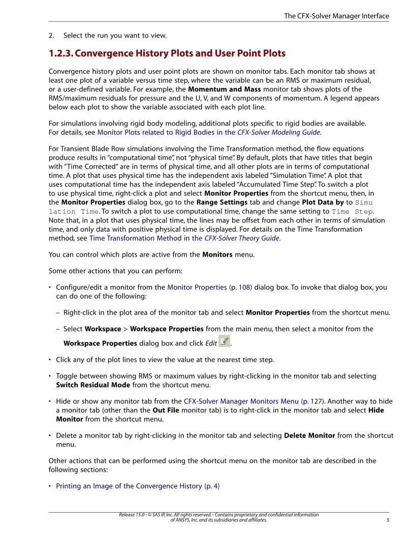
2. Select the run you want to view.
1.2.3. Convergence History Plots and User Point Plots
Convergence history plots and user point plots are shown on monitor tabs. Each monitor tab shows atleast one plot of a variable versus time step, where the variable can be an RMS or maximum residual,or a user-defined variable. For example, the Momentum and Mass monitor tab shows plots of theRMS/maximum residuals for pressure and the U, V, and W components of momentum. A legend appearsbelow each plot to show the variable associated with each plot line.
For simulations involving rigid body modeling, additional plots specific to rigid bodies are available.For details, see Monitor Plots related to Rigid Bodies in the CFX-Solver Modeling Guide.
For Transient Blade Row simulations involving the Time Transformation method, the flow equationsproduce results in “computational time”, not “physical time”. By default, plots that have titles that beginwith “Time Corrected” are in terms of physical time, and all other plots are in terms of computationaltime. A plot that uses physical time has the independent axis labeled “Simulation Time”. A plot thatuses computational time has the independent axis labeled “Accumulated Time Step”. To switch a plotto use physical time, right-click a plot and select Monitor Properties from the shortcut menu, then, inthe Monitor Properties dialog box, go to the Range Settings tab and change Plot Data by to Simulation Time . To switch a plot to use computational time, change the same setting to Time Step .Note that, in a plot that uses physical time, the lines may be offset from each other in terms of simulationtime, and only data with positive physical time is displayed. For details on the Time Transformationmethod, see Time Transformation Method in the CFX-Solver Theory Guide.
You can control which plots are active from the Monitors menu.
Some other actions that you can perform:
• Configure/edit a monitor from the Monitor Properties (p. 108) dialog box. To invoke that dialog box, youcan do one of the following:
– Right-click in the plot area of the monitor tab and select Monitor Properties from the shortcut menu.
– Select Workspace > Workspace Properties from the main menu, then select a monitor from the
Workspace Properties dialog box and click Edit .
• Click any of the plot lines to view the value at the nearest time step.
• Toggle between showing RMS or maximum values by right-clicking in the monitor tab and selectingSwitch Residual Mode from the shortcut menu.
• Hide or show any monitor tab from the CFX-Solver Manager Monitors Menu (p. 127). Another way to hidea monitor tab (other than the Out File monitor tab) is to right-click in the monitor tab and select Hide
Monitor from the shortcut menu.
• Delete a monitor tab by right-clicking in the monitor tab and selecting Delete Monitor from the shortcutmenu.
Other actions that can be performed using the shortcut menu on the monitor tab are described in thefollowing sections:
• Printing an Image of the Convergence History (p. 4)
3Release 15.0 - © SAS IP, Inc. All rights reserved. - Contains proprietary and confidential information
of ANSYS, Inc. and its subsidiaries and affiliates.
The CFX-Solver Manager Interface
• Saving a Picture of the Convergence History (p. 4)
• Exporting Plot Data (p. 4)
• Exporting Monitor Data from the Command Line (p. 5)
1.2.3.1. Printing an Image of the Convergence History
You can print a picture of the convergence history plot:
1. Right-click in the convergence history plot and select Print.
The Print dialog box appears.
2. Configure the printer as required.
3. Click Print.
1.2.3.2. Saving a Picture of the Convergence History
You can save a picture of the convergence history plot:
1. Right-click in the convergence history plot and select Save Picture.
The Image File dialog box appears.
2. In the Image File dialog box, select a location to which to export the image.
3. Under File name, enter the name for the file.
4. Under File type, select the format to export.
5. Click Save.
1.2.3.3. Exporting Plot Data
Data from any plot monitor can be exported. The data format for the exported file consists of comma-delimited entries. This data can be used as the basis for import to another application.
1. Right-click in the convergence history plot and select Export Plot Data.
The Export dialog box appears.
2. Select a location to which to export the data.
3. Under File name, enter the name for the file.
4. Under File Type, select the format to export.
Files are saved with a .csv extension by default, but this can be modified as required.
5. Click Save.
Release 15.0 - © SAS IP, Inc. All rights reserved. - Contains proprietary and confidential informationof ANSYS, Inc. and its subsidiaries and affiliates.4
CFX-Solver Manager Basics
The data from each plotted variable is exported to the specified file.
Note
Monitor data can also be exported using the command-line application cfx5mondata .
Note
When exporting from a time-corrected plot, you can export data (one or more variables) foronly one monitor point; each selected plot line variable must belong to the same monitorpoint. This restriction guarantees that all exported data is written in terms of the same cor-rected time. You can change which plot line variables are selected by using the Monitor
Properties dialog box (right-click in the plot area and select Monitor Properties from theshortcut menu).
1.2.3.4. Exporting Monitor Data from the Command Line
The cfx5mondata application provides a command-line driven mechanism to query or extract monitordata from the directory in which a solver run is executing, a CFX-Solver Results file, or a monitor file.When extracted, monitor data are written in a comma-separated format that is similar to the outputgenerated by the Exporting Plot Data capability.
To obtain a complete list of available command line options for cfx5mondata type the followingcommand into a UNIX terminal or a suitable Windows command line and press Return or Enter:
cfx5mondata -help
1.2.4. Text Output Window
The text output window is a monitor tab that lists simulation information and the progress of a solution,including information such as physical properties, boundary conditions, and various other parametersused or calculated in creating the model. The source of the displayed information is an output file froma solver run. For details, see CFX-Solver Output File (p. 38).
For an ANSYS Multi-field run, an additional text output window shows text output from the ANSYSsolver. In this case, you can switch between viewing the CFX output file and the ANSYS output file byusing the tabs at the top of the window. For details on ANSYS Multi-field runs, see Coupling CFX to anExternal Solver: ANSYS Multi-field Simulations.
You can hide or show the Out File monitor tab from the CFX-Solver Manager Monitors Menu (p. 127).
Right-click in the Out File monitor tab to access a shortcut menu with commands for finding text, se-lecting text, copying text, saving the text to a file, managing bookmarks, editing the properties of theOut File monitor tab, and deleting the Out File monitor tab.
The following sections explain some of these actions in more detail:
• Searching for Text (p. 6)
• Saving the Text to File (p. 6)
5Release 15.0 - © SAS IP, Inc. All rights reserved. - Contains proprietary and confidential information
of ANSYS, Inc. and its subsidiaries and affiliates.
The CFX-Solver Manager Interface

1.2.4.1. Searching for Text
The output window can be searched for specific text:
1. Right-click in the text output window and select Find.
2. In Find, enter words to find.
3. Select or clear the Case Sensitive check box.
4. Click Previous or Next to search up or down from the current location. An icon will appear to the leftof the Find label if the text could not be found in the file when searching in the selected direction fromthe current location.
1.2.4.2. Saving the Text to File
The text of the output window can be saved to file (even when a run is in progress):
1. Right-click in the text output window.
2. Select Save As.
3. Select a file location to save the text file.
4. Enter a file name for the text file.
5. Click Save.
1.2.5. Multi-Configuration Run History Page
A multi-configuration simulation has several workspaces:
• One workspace for each analysis. Each of these workspaces has a convergence history plot and a textoutput window that resemble those of a single-analysis simulation.
• One workspace that shows an overview of the multi-configuration simulation. There is a run history page
that lists each simulation step (analysis) and its overall status ( = in progress, = complete, = error),and a text output window that provides the status of each simulation step.
A sample run history page is shown below:
Release 15.0 - © SAS IP, Inc. All rights reserved. - Contains proprietary and confidential informationof ANSYS, Inc. and its subsidiaries and affiliates.6
CFX-Solver Manager Basics
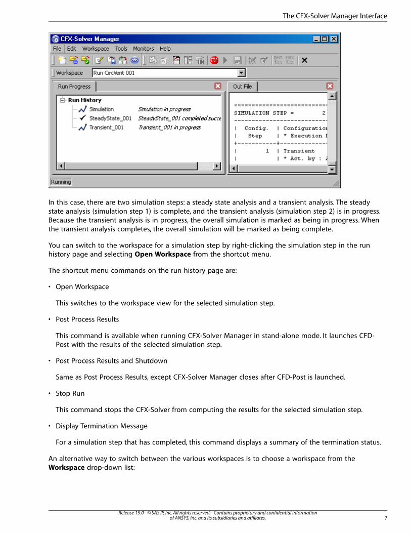
In this case, there are two simulation steps: a steady state analysis and a transient analysis. The steadystate analysis (simulation step 1) is complete, and the transient analysis (simulation step 2) is in progress.Because the transient analysis is in progress, the overall simulation is marked as being in progress. Whenthe transient analysis completes, the overall simulation will be marked as being complete.
You can switch to the workspace for a simulation step by right-clicking the simulation step in the runhistory page and selecting Open Workspace from the shortcut menu.
The shortcut menu commands on the run history page are:
• Open Workspace
This switches to the workspace view for the selected simulation step.
• Post Process Results
This command is available when running CFX-Solver Manager in stand-alone mode. It launches CFD-Post with the results of the selected simulation step.
• Post Process Results and Shutdown
Same as Post Process Results, except CFX-Solver Manager closes after CFD-Post is launched.
• Stop Run
This command stops the CFX-Solver from computing the results for the selected simulation step.
• Display Termination Message
For a simulation step that has completed, this command displays a summary of the termination status.
An alternative way to switch between the various workspaces is to choose a workspace from theWorkspace drop-down list:
7Release 15.0 - © SAS IP, Inc. All rights reserved. - Contains proprietary and confidential information
of ANSYS, Inc. and its subsidiaries and affiliates.
The CFX-Solver Manager Interface

In the drop-down list, the analyses of a multi-configuration simulation are listed below the name of therun, and are indented to show that they belong to the run. Selecting the name of the run switches tothe run history page.
1.3. Customizing CFX-Solver Manager
The size and position of most windows in CFX-Solver Manager can be changed to customize the appear-ance, function and placement of objects. Toolbars can also be moved as required; just click and dragthe left edge of a toolbar to a new position. (The toolbar orients itself vertically if places along the leftor right side of the application.)
Settings such as window sizes, selected plot variables, and other settings specific to the current viewcan be saved as a layout file (*.mst ). For example, you could select a plot variable and configure thecurrent view. You could then save the layout and restore it at a later time. For details, see CFX-SolverManager Workspace Menu (p. 105).
Release 15.0 - © SAS IP, Inc. All rights reserved. - Contains proprietary and confidential informationof ANSYS, Inc. and its subsidiaries and affiliates.8
CFX-Solver Manager Basics

Chapter 2: Working with Solver Manager
This chapter describes procedures for starting specific types of runs using CFX-Solver Manager. Thesteps to take depend on whether an initial values file is required or not, and whether the CFX-Solverinput file name has already been passed to the CFX-Solver Manager.
This chapter describes:2.1. Solver Run Overview2.2.The Define Run Dialog Box2.3. Run Output Results2.4. Parallel Run2.5. Restarting a Run2.6. ANSYS Multi-field Run
2.1. Solver Run Overview
To run a case, review the settings in the File > Define Run dialog box. The number of settings that youneed to change or specify depends on the case:
• In some cases, you need only to specify the name of a CFX-Solver input file (*.def or *.mdef ). For casesthat require initialization from previous results, you also need to specify the name of a results file (*.resor *.mres ).
• You can choose to run in serial or parallel:
– Serial run is the default way of running a CFD case. During a serial run, all computation is done by asingle process running on one processor.
– Parallel run divides computation into more than one process and is done on more than one processorin a single machine (local parallel processing) or on more than one machine (distributed parallel pro-cessing).
• You can configure an ANSYS Multi-field run, which enables the coupling of the CFX-Solver with the ANSYSSolver in order to execute cases that require two-way fluid-structure interaction.
• For simulations with multiple configurations, you can make global and configuration specific settings.Note that ANSYS Multi-field runs are not supported for multi-configuration simulations.
When you have finished setting up the case, click Start Run.
Tip
In ANSYS Workbench you have the option of clicking Save Settings to save the settings ofthe Define Run dialog box to the Solution cell (some of these settings are visible in theSolution cell's Properties). By saving the settings in this way, you can configure the run fromCFX-Solver Manager, but start the run from ANSYS Workbench (by updating the Solutioncell).
9Release 15.0 - © SAS IP, Inc. All rights reserved. - Contains proprietary and confidential information
of ANSYS, Inc. and its subsidiaries and affiliates.
Details of making these changes with the Define Run dialog box are described in the next section.
2.2. The Define Run Dialog Box
You access the Define Run dialog box from CFX-Solver Manager by clicking File > Define Run.
The tabs of the Define Run dialog box that can be configured are described in the following sections:2.2.1. Run Definition Tab2.2.2. Initial Values Tab2.2.3. MultiField Tab2.2.4. Partitioner Tab2.2.5. Solver Tab2.2.6. Interpolator Tab2.2.7. Configuring Memory for the CFX-Solver
2.2.1. Run Definition Tab
To configure the run definition tab:
Under Solver Input File, ensure that the name of a CFX-Solver input file (with extension .def or.mdef ) is specified.
The name will be set automatically if:
• You have started CFX-Solver Manager using the Define Run action in CFX-Pre.
• You have started CFX-Solver Manager from the command line using the -interactive and -def or-mdef options. For details, see Starting the CFX-Solver from the Command Line in the CFX-Solver Manager
User's Guide.
CFX-Solver input file names must not contain spaces when run with an associated ANSYS input file(.inp ). Note that in CFX-Solver Manager, when specifying or editing the Solver Input File by typing
from the keyboard, you must click Reload run settings from file to have the changes take effect.
In CFX-Solver Manager, if a multi-configuration definition or results file (*.mdef or *.mres , respectively)is selected as the CFX-Solver Input file, then the settings on the tabs described below can be made ona simulation-wide or per-configuration basis. This is done by choosing either Global Settings ora specific configuration name for the Edit Configuration option. Note that when global settings aremade, they are inherited by all configurations. You can then override any setting for a specific config-uration, but it is important to note that in this situation the remainder of the settings for the configur-ation will not be inherited from the global settings.
• Set Type of Run to Full or Partitioner Only .
– Full runs the partitioner if applicable, and then runs the solver.
– Partitioner Only is used for parallel runs only and does not run the solver. This writes a .parfile.
• You can select or clear Double Precision. This setting will determine the default (single or double) precisionof the partitioner, solver, and interpolator executables. For details on the precision of executables, seeDouble-Precision Executables in the CFX-Solver Manager User's Guide. The precisions of the partitioner,solver, and interpolator executables can be optionally overridden individually on the Partitioner, Solver,and Interpolator tabs.
Release 15.0 - © SAS IP, Inc. All rights reserved. - Contains proprietary and confidential informationof ANSYS, Inc. and its subsidiaries and affiliates.10
Working with Solver Manager
• You can configure the Parallel Environment as required (see below).
• If required, you can set the working directory under Run Environment.
• If required, you can select Show Advanced Controls to display other tabs.
Parallel Environment
Under Parallel Environment, select a Run Mode option. The run mode determines whether the runis serial (the default when defining a run in which a problem is solved as one process), or parallel(problem is split into partitions).
• A serial run (the default) requires no additional configuration.
• For a local parallel run, specify the number of partitions. This value is the number of separate processesthat will be executed.
• For a distributed parallel run, specify the number of partitions assigned to each host. If choosing a specifiedpartition weighting (under the Partitioner tab), click directly on the partition weight number to edit it.There should be one weight entry per partition.
For more information on Parallel Processing, see Parallel Run in the CFX-Solver Manager User's Guide.
2.2.2. Initial Values Tab
The Initial Values tab is used for specifying initial values via results files.
If you do not specify initial values via results files, the software will use initialization data from (in orderof precedence):
• In CFX-Pre on the Initialization tab in the Domain details view
• In CFX-Pre on the Initialization tab in the Global Initialization details view
• Automatically generated initial values
However, automatically generated initial values may not be suitable for some steady-state cases andare insufficient for all transient cases
If you do specify initial values via results files, those values will override any initial values listed above,as applicable.
You can set initial values via results files in a variety of places as listed here (in order of precedence):
• In CFX-Solver Manager in the Define Run dialog box on the Initial Values tab
• In CFX-Pre in the Configuration details view on the Initial Values tab
Note that for cases with multiple configurations, initial values cannot be set globally (i.e. in CFX-Solver Manager or in CFX-Pre in the Execution Control details view); they can only be set per config-uration (i.e. in CFX-Pre in the Configuration details view).
• In CFX-Pre in the Execution Control details view on the Initial Values tab
You can set initial values via results files as follows:
11Release 15.0 - © SAS IP, Inc. All rights reserved. - Contains proprietary and confidential information
of ANSYS, Inc. and its subsidiaries and affiliates.
The Define Run Dialog Box

1. Under the Initial Values tab, select the Initial Values Specification check box to show the initial valuessettings.
2. Click New to create an initial values object.
3. Select an initial values object from the list and select either the Results File or Configuration Results
option for Initial Values > Option.
• If you selected the Results File option, then specify the file name of a file from which initial valuesshould be used.
• If you selected the Configuration Results option, then specify the name of the configuration fromwhich initial values should be used. Note that this option is only available in the context of multi-configuration simulations. It allows the introduction of dependencies on initial values that will becomeavailable at run time.
Additional information is provided in Initial Condition Modeling in the CFX-Solver Modeling Guide.
4. Optionally specify Interpolation Mapping settings in order to select, position, and/or replicate thedata. For details, see Interpolation Mapping in the CFX-Solver Modeling Guide.
5. Select Continue History From if you want to continue the run history (convergence history, monitorplots, time and time step counters, etc…) and use the smoothest restart possible from the selectedInitial Values File. The run will continue from the one contained in the specified initial values object.Note that the run history will reset if Continue History From is not selected.
6. The Use Mesh From setting determines which mesh is used for the analysis: the one specified in theSolver Input File option, or the one in the Initial Values file. The mesh from the Initial Values File canonly be used in a limited set of circumstances. See Using the Mesh from the Initial Values File in theCFX-Solver Modeling Guide for details.
Full details for Initial Values Files can be found in Reading the Initial Conditions from a File in the CFX-
Solver Modeling Guide.
2.2.3. MultiField Tab
The MultiField tab is used for launching ANSYS Multi-field runs and only appears if the specified CFX-Solver input file has External Solver Coupling set to ANSYS MultiField or ANSYS Multifieldvia Prep7 . When this setting is enabled, the CFX-Solver Manager can be used to launch a completeANSYS Multi-field run, including processing the multi-field commands (where appropriate) andlaunching CFX and ANSYS solvers. For details, see Pre-Processing in the CFX-Solver Modeling Guide. Adescription of the different run modes and settings can be found in ANSYS Multi-field Run in the CFX-
Solver Manager User's Guide.
The following table outlines various settings available on MultiField tab. The settings are marked as re-quired or optional based on the MFX run mode chosen for the ANSYS Multi-field run.
Release 15.0 - © SAS IP, Inc. All rights reserved. - Contains proprietary and confidential informationof ANSYS, Inc. and its subsidiaries and affiliates.12
Working with Solver Manager
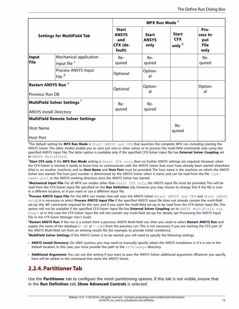
MFX Run Mode a
Settings for MultiField Tab
Pro-
cess In-
put
File
only
Start
CFX
onlyb
Start
ANSYS
only
Start
ANSYS
and
CFX (de-
fault)
Re-quired
Re-quired
Re-quired
Mechanical application
input file c
Input
File
Option-al
OptionalProcess ANSYS Input
File d
Option-al
Option-al
OptionalRestart ANSYS Run
e
Previous Run DB
Re-quired
Re-quired
MultiField Solver Settingsf
ANSYS Install Directory
Re-quired
MultiField Remote Solver Settings
Host Name
Host PortaThe default setting for MFX Run Mode is Start ANSYS and CFX that launches the complete MFX run, including starting theANSYS Solver. The other modes enable you to start just one or other solver, or to process the multi-field commands only using thespecified ANSYS Input File. The latter option is available only if the specified CFX-Solver input file has External Solver Coupling setto ANSYS MultiField .b
Start CFX only: If the MFX Run Mode setting is Start CFX only , then no further ANSYS settings are required. However, whenthe CFX-Solver is started, it needs to know how to communicate with the ANSYS Solver that must have already been started elsewhere(that is, on another machine), and so Host Name and Host Port must be provided. The host name is the machine on which the ANSYSSolver was started. The host port number is determined by the ANSYS Solver when it starts, and can be read from the file <job-name>.port in the ANSYS working directory once the ANSYS Solver has started.cMechanical Input File: For all MFX run modes other than Start CFX only , the ANSYS input file must be provided. This will be
read from the CFX-Solver input file specified on the Run Definition tab; however, you may choose to change this if the file is nowin a different location, or if you want to use a different input file.d
Process ANSYS Input File: For the MFX run modes that will start the ANSYS Solver (Start ANSYS and CFX and Start ANSYSonly ), it is necessary to select Process ANSYS Input File if the specified ANSYS input file does not already contain the multi-fieldset-up (the MF commands required for the run), and if you want the multi-field set-up to be read from the CFX-Solver input file. Thisoption will not be available if the specified CFX-Solver input file has External Solver Coupling set to ANSYS MultiField viaPrep7 , as in this case the CFX-Solver input file will not contain any multi-field set-up. For details, see Processing the ANSYS InputFile in the CFX-Solver Manager User's Guide.eRestart ANSYS Run: If the run is a restart from a previous ANSYS Multi-field run, then you need to select Restart ANSYS Run and
supply the name of the database (*.db or *.rdb ) from the previous run. This is not necessary if you are starting the CFX part ofthe ANSYS Multi-field run from an existing results file (for example, to provide initial conditions).fMultiField Solver Settings: If the ANSYS Solver is to be started, you will need to specify the following settings:
• ANSYS Install Directory: On UNIX systems, you may need to manually specify where the ANSYS installation is if it is not in thedefault location. In this case, you must provide the path to the v150/ansys directory.
• Additional Arguments: You can use this setting if you want to pass the ANSYS Solver additional arguments. Whatever you specifyhere will be added to the command that starts the ANSYS Solver.
2.2.4. Partitioner Tab
Use the Partitioner tab to configure the mesh partitioning options. If this tab is not visible, ensure thatin the Run Definition tab, Show Advanced Controls is selected.
13Release 15.0 - © SAS IP, Inc. All rights reserved. - Contains proprietary and confidential information
of ANSYS, Inc. and its subsidiaries and affiliates.
The Define Run Dialog Box
• You can select a partition file to load by clicking Browse beside Initial Partition File. The *.par file
is only available if a model has already been partitioned. The number of partitions in the partitioning filemust be the same as on the Run Definition tab.
Note
An existing partition file cannot be used if the simulation involves either the Monte Carloor Discrete Transfer radiation model. Partitions may be viewed prior to running CFX-Solver.For details, see CFX Partition File in the CFX-Solver Manager User's Guide.
• Under Run Priority, you can select Idle , Low, Standard or High . For a discussion of these priorities,see The cfx5control Application in the CFX-Solver Manager User's Guide.
• You can override the precision set on the Run Definition tab by selecting Override Default Precision
and then setting the precision. For details on the precision of executables, see Double-Precision Executablesin the CFX-Solver Manager User's Guide.
• If required, you can select the Use Large Problem Partitioner option, which is available on 64-bit platformsonly. This option starts the large problem partitioner which can handle problems of up to 2 billion elements;the standard partitioner can only handle problems up to 2^31-1 words (80 million unstructured elements).This partitioner uses 64-bit integer and logical variables so it will allocate more memory than the defaultpartitioning executable. For details, see Large Problem Partitioner Executables in the CFX-Solver Manager
User's Guide.
• Under Partitioning Detail, you can choose a Partition Type and configure it.
Depending on the selected partition type, various options must be configured. Partition types include:
– Multilevel Graph Partitioning Software - MeTiS in the CFX-Solver Modeling Guide. When first running inparallel, it is recommended that Partition Type be set to MeTiS.
– Optimized Recursive Coordinate Bisection in the CFX-Solver Modeling Guide
– Recursive Coordinate Bisection in the CFX-Solver Modeling Guide
– Directional Recursive Coordinate Bisection in the CFX-Solver Modeling Guide
– User Specified Direction in the CFX-Solver Modeling Guide
– Radial in the CFX-Solver Modeling Guide
– Circumferential in the CFX-Solver Modeling Guide
– Simple Assignment in the CFX-Solver Modeling Guide
• If required, you can configure the Partition Weighting as described below.
• If required, you can configure the Multidomain Option. You can select from the following options:
– Independent Partitioning : Each domain is partitioned independently into the specified numberof partitions.
Release 15.0 - © SAS IP, Inc. All rights reserved. - Contains proprietary and confidential informationof ANSYS, Inc. and its subsidiaries and affiliates.14
Working with Solver Manager
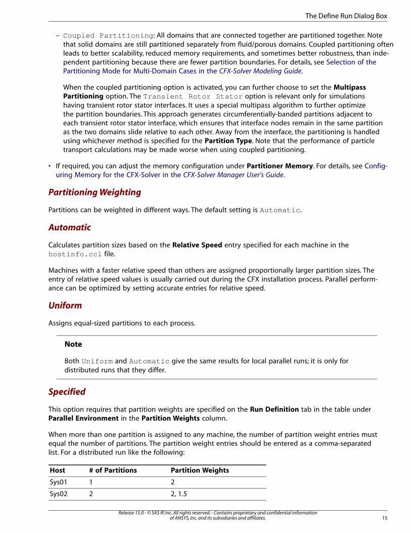
– Coupled Partitioning : All domains that are connected together are partitioned together. Notethat solid domains are still partitioned separately from fluid/porous domains. Coupled partitioning oftenleads to better scalability, reduced memory requirements, and sometimes better robustness, than inde-pendent partitioning because there are fewer partition boundaries. For details, see Selection of thePartitioning Mode for Multi-Domain Cases in the CFX-Solver Modeling Guide.
When the coupled partitioning option is activated, you can further choose to set the Multipass
Partitioning option. The Transient Rotor Stator option is relevant only for simulationshaving transient rotor stator interfaces. It uses a special multipass algorithm to further optimizethe partition boundaries. This approach generates circumferentially-banded partitions adjacent toeach transient rotor stator interface, which ensures that interface nodes remain in the same partitionas the two domains slide relative to each other. Away from the interface, the partitioning is handledusing whichever method is specified for the Partition Type. Note that the performance of particletransport calculations may be made worse when using coupled partitioning.
• If required, you can adjust the memory configuration under Partitioner Memory. For details, see Config-uring Memory for the CFX-Solver in the CFX-Solver Manager User's Guide.
Partitioning Weighting
Partitions can be weighted in different ways. The default setting is Automatic .
Automatic
Calculates partition sizes based on the Relative Speed entry specified for each machine in thehostinfo.ccl file.
Machines with a faster relative speed than others are assigned proportionally larger partition sizes. Theentry of relative speed values is usually carried out during the CFX installation process. Parallel perform-ance can be optimized by setting accurate entries for relative speed.
Uniform
Assigns equal-sized partitions to each process.
Note
Both Uniform and Automatic give the same results for local parallel runs; it is only fordistributed runs that they differ.
Specified
This option requires that partition weights are specified on the Run Definition tab in the table underParallel Environment in the Partition Weights column.
When more than one partition is assigned to any machine, the number of partition weight entries mustequal the number of partitions. The partition weight entries should be entered as a comma-separatedlist. For a distributed run like the following:
Partition Weights# of PartitionsHost
21Sys01
2, 1.52Sys02
15Release 15.0 - © SAS IP, Inc. All rights reserved. - Contains proprietary and confidential information
of ANSYS, Inc. and its subsidiaries and affiliates.
The Define Run Dialog Box
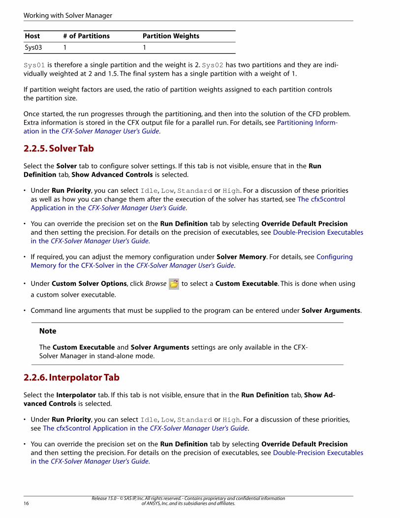
Partition Weights# of PartitionsHost
11Sys03
Sys01 is therefore a single partition and the weight is 2. Sys02 has two partitions and they are indi-vidually weighted at 2 and 1.5. The final system has a single partition with a weight of 1.
If partition weight factors are used, the ratio of partition weights assigned to each partition controlsthe partition size.
Once started, the run progresses through the partitioning, and then into the solution of the CFD problem.Extra information is stored in the CFX output file for a parallel run. For details, see Partitioning Inform-ation in the CFX-Solver Manager User's Guide.
2.2.5. Solver Tab
Select the Solver tab to configure solver settings. If this tab is not visible, ensure that in the Run
Definition tab, Show Advanced Controls is selected.
• Under Run Priority, you can select Idle , Low, Standard or High . For a discussion of these prioritiesas well as how you can change them after the execution of the solver has started, see The cfx5controlApplication in the CFX-Solver Manager User's Guide.
• You can override the precision set on the Run Definition tab by selecting Override Default Precision
and then setting the precision. For details on the precision of executables, see Double-Precision Executablesin the CFX-Solver Manager User's Guide.
• If required, you can adjust the memory configuration under Solver Memory. For details, see ConfiguringMemory for the CFX-Solver in the CFX-Solver Manager User's Guide.
• Under Custom Solver Options, click Browse to select a Custom Executable. This is done when using
a custom solver executable.
• Command line arguments that must be supplied to the program can be entered under Solver Arguments.
Note
The Custom Executable and Solver Arguments settings are only available in the CFX-Solver Manager in stand-alone mode.
2.2.6. Interpolator Tab
Select the Interpolator tab. If this tab is not visible, ensure that in the Run Definition tab, Show Ad-
vanced Controls is selected.
• Under Run Priority, you can select Idle , Low, Standard or High . For a discussion of these priorities,see The cfx5control Application in the CFX-Solver Manager User's Guide.
• You can override the precision set on the Run Definition tab by selecting Override Default Precision
and then setting the precision. For details on the precision of executables, see Double-Precision Executablesin the CFX-Solver Manager User's Guide.
Release 15.0 - © SAS IP, Inc. All rights reserved. - Contains proprietary and confidential informationof ANSYS, Inc. and its subsidiaries and affiliates.16
Working with Solver Manager
• If required, under Interpolator Memory, you can adjust the memory configuration. For details, see Con-figuring Memory for the CFX-Solver in the CFX-Solver Manager User's Guide.
• You can select Domain Search Control to access the Bounding Box Tolerance setting (see below).
• You can select Interpolation Model Control to access the Enforce Strict Name Mapping for Phases
(only available in CFX-Solver Manager), Particle Relocalization Tolerance (only available in CFX-SolverManager), and Mesh Deformation Option settings (see below).
The Bounding Box Tolerance and Particle Relocalization Tolerance settings are described in Adjustingthe Bounding Box Tolerance in the CFX-Solver Modeling Guide.
The Enforce Strict Name Mapping for Phases setting controls how fluids are mapped between theInitial Values files and the Solver Input File. By default, when interpolating from multiple Initial Valuesfiles onto a single Solver Input File, if each Initial Values file contains just one fluid, then the CFX-Inter-polator regards all of these fluids as being the same fluid, regardless of the Fluid Definition name. Youcan change this default behavior by turning on the Enforce Strict Name Mapping for Phases setting.This forces the CFX-Interpolator to use the Fluid Definition names to match each fluid from each InitialValues file with the appropriate fluid in the Solver Input File.
The Mesh Deformation Option setting controls which mesh in the Initial Values File is used to checkthe mesh displacements: the initial mesh or the final mesh. The options are Automatic , Use LatestMesh, and Use Initial Mesh . When the Automatic option is selected, the initial mesh will beused if the Continue History From check box is selected, and the latest mesh will be used if the Con-
tinue History From check box is cleared.
2.2.7. Configuring Memory for the CFX-Solver
There may be instances when the CFX-Solver fails due to insufficient memory. You can determine thatthe CFX-Solver failed in this way as well as which of the interpolator, partitioner, or flow solver stepsfailed by reviewing the CFX-Solver output file. In this case you will be required to adjust the memoryconfiguration of the appropriate CFX-Solver step. The methods available for adjusting memory are:
• Memory Allocation Factor: Use this method to modify the memory allocation for the CFX-Solver step asa whole. For example, a value of 1.05 for Memory Allocation Factor increases memory allocation by 5%and a value of 1.1 increases memory allocation by 10%.
• Detailed Memory Overrides: Use this method to adjust Real Memory, Integer Memory, Character
Memory, Double Memory and Logical Memory as required.
• The number of words of memory can be specified, or a memory multiplier can be used. Use a unit of Mfor mega-words, K for kilo-words, or X for a memory multiplier. For example, 2 X doubles the memory al-location and 15 M means 15 million words of memory. If a value is not specified for a particular type ofmemory, the value calculated by the Solver is used. If a value is entered, it overrides the automatic estimatemade by the Solver.
• Catalogue Size Override: If the solver fails with an *.out file containing the error message *** INSUFFICIENT CATALOGUE SIZE *** , increase the Catalogue Size Override setting to a value above 1until the solver runs. This parameter has the same syntax as the Detailed Memory Overrides above. Forexample, you can scale the default size by using a scale factor greater than 1, such as 1.05 X. For details,see Starting the CFX-Solver from the Command Line (p. 129).
17Release 15.0 - © SAS IP, Inc. All rights reserved. - Contains proprietary and confidential information
of ANSYS, Inc. and its subsidiaries and affiliates.
The Define Run Dialog Box
2.3. Run Output Results
Once the run definition is complete and the run is started, a new workspace is created and the Work-
space drop-down list will contain an entry based on the name of the Solver Input File. For example,using the Solver Input File named case.def , the workspace entry will be similar to Run case 001 .Note that the integer index is identical to the index used for the text output and result files for the run.For multi-configuration simulations, one additional workspace is created as each new configuration isexecuted. The Workspace drop-down list will contain entries based on the names of the configurations.
Most workspaces contain a mixture of plot and text output monitors that are updated by the CFX-Solver as the simulation progresses. By default, appropriate monitors are automatically created in theworkspace for the particular type of simulation you are running. These include:
• Plot monitors showing the normalized residuals (which should decrease as the solution progresses)for each equation being solved, plus any user-defined monitor values.
• A text monitor showing the contents of the CFX-Solver output file. For details, see CFX-Solver OutputFile (p. 38).
No plot monitors are generated for the simulation-level workspace (named according to the Solver
Input File) created for multi-configuration simulations. This workspace includes one text monitor,showing the contents of the CFX Multi-Configuration output File. For details, see CFX Multi-ConfigurationOutput File (p. 77).
When the CFX-Solver stops running, a dialog box is displayed that indicates whether the run completednormally or not, and additional information regarding the reasons for terminating the run are presentedin the text output window.
The following dialog boxes may appear:
• Solver Run Finished Normally
• Solver Run Stopped By User
• Solver Run Terminated With Errors
To close the dialog box without post-processing the results, click OK.
On the Solver Run Finished Normally and Solver Run Stopped By User dialog boxes, you can choosefrom the following options:
Post-Process Results
Opens CFD-Post with the specified CFX-Solver Results file loaded.
Multi-Configuration Load Options
If this option is available, you can use it to control how the results of a multi-configuration run are loaded,or to load just the last case of such a run.
Select a multi-configuration load option to control how you load a multi-configuration (.mres ) fileor a results file (.res ) that contains a run history (that is, a file that was produced from a definitionfile that had its initial values specified from a results file from a previous run and saved to the resultsfile that you are loading). Choose:
• Single Case to load all configurations of a multi-configuration run as a single case, or all of the resultshistory from a results file that contains a run history. In either case, only one set of results will appear
Release 15.0 - © SAS IP, Inc. All rights reserved. - Contains proprietary and confidential informationof ANSYS, Inc. and its subsidiaries and affiliates.18
Working with Solver Manager

in the viewer, but you can use the timestep selector to move between results. This option is not fullysupported.
• Separate Cases to load all configurations from a multi-configuration run into separate cases. If a resultsfile with run history is loaded, CFD-Post loads the results from this file and the results for any resultsfile in its run history as separate cases. Each result appears as a separate entry in the tree.
• Last Case to load only the last configuration of a multi-configuration results file, or only the last resultsfrom a results file that contains a run history.
Shut down CFX-Solver Manager
Shuts down CFX-Solver Manager before CFD-Post is launched. This minimizes the number of licensesyou use concurrently.
To post-process the results, make the desired settings on the dialog box and click OK.
After a run has finished you can use CFX-Solver Manager to:
• Define a new run by following the earlier procedure. For details, see Define Run Command (p. 99)
• Calculate more timesteps for the original run. For details, see Restarting a Run (p. 22).
• View results in CFD-Post (provided that the CFX-Solver produced a results file and did not fail). For details,see Overview of CFD-Post in the CFD-Post User's Guide.
• Print residual plots in the convergence history plots. For details, see Printing an Image of the ConvergenceHistory (p. 4).
• Add comments to the saved version of the text in the text output window. For details, see Starting theCFX-Solver from the Command Line (p. 129).
• Export results in a format suitable for post-processors other than CFD-Post. For details, see File ExportUtility (p. 155).
• Quit CFX-Solver Manager by selecting File > Quit. This does not stop the CFX-Solver calculation. Additionally,CFX-Solver Manager can be reopened at any time. For details, see CFX-Solver Manager File Menu (p. 99).
The CFX Tutorials describe how to use the CFX-Solver Manager step-by-step for several different cases.If you are a new user, you should try at least the first few tutorials.
2.4. Parallel Run
Note
CFX-Solver can be run in parallel only if an appropriate license has been purchased.
Information on a parallel run is explained in more detail:
• Overview (p. 20)
• General Procedure (p. 20)
• Configuring a Parallel Run (p. 20)
19Release 15.0 - © SAS IP, Inc. All rights reserved. - Contains proprietary and confidential information
of ANSYS, Inc. and its subsidiaries and affiliates.
Parallel Run
2.4.1. Overview
There are several parallel run modes, including MPI (Message Passing Interface) and PVM (Parallel VirtualMachine) communication libraries. Both are simply libraries that enable the flow solver processes tocommunicate with each other. Proprietary, vendor specific versions of MPI are available on 64-bit Linuxand support a wider array of high speed network devices, as well as Shared Memory communication.
General information on setting up a parallel run and advice on obtaining optimal parallel performanceis available in Using the Solver in Parallel in the CFX-Solver Modeling Guide.
Individual machines may need to be configured to run in parallel.
2.4.2. General Procedure
To run CFX-Solver in parallel, the following procedure must be followed:
1. Partition the mesh into the appropriate number of partitions.
2. Run CFX-Solver on the partitioned problem.
These two jobs can be done either as one composite run, or as two separate jobs.
2.4.3. Configuring a Parallel Run
Under Run Mode, select a parallel method:
• Local Parallel Setup (p. 20)
• Distributed Parallel Setup (p. 20)
2.4.3.1. Local Parallel Setup
Select a local parallel run if running a problem with two or more processors on the local machine.
Any number of partitions between 2 and 16384 can be selected. When running the job in the CFX-Solver, the computation is divided into this number of processes. For details, see Partitioner Tab (p. 13).The solver enables further changes. For details, see Solver Tab (p. 16).
1. Select one of the local parallel run modes (for example, Platform MPI Local Parallel ). Whichparallel run modes you can select depends on the hardware and operating system on which you arerunning.
2. Click Add Partition or Remove Partition to increase or decrease the number of partitions.
Partitions may need to be configured based on partition weighting. For details, see PartitionerTab (p. 13).
2.4.3.2. Distributed Parallel Setup
Select a distributed parallel option to run a problem on two or more computers.
Release 15.0 - © SAS IP, Inc. All rights reserved. - Contains proprietary and confidential informationof ANSYS, Inc. and its subsidiaries and affiliates.20
Working with Solver Manager
2.4.3.2.1. Overview
To configure a distributed parallel run, a file named hostinfo.ccl must exist in the <CFXROOT>/con-fig/ CFX directory on the master node and be readable by all users of the software. This file is adatabase containing information about available nodes and where ANSYS CFX is installed on each ofthem. See hostinfo.ccl file in the Installation and Licensing Documentation (Windows) or hostinfo.ccl Filein the Installation and Licensing Documentation (UNIX/Linux) for more details.
Note
• Including hosts in the hostinfo.ccl file is optional. If you want to use a host that is notpresent in either the hostinfo.ccl file in the <CFXROOT>/config/ directory or your ownversion of this file, then you can add this host to the list that is used for a particular run byusing the CFX-Solver Manager as described in Selecting Parallel Hosts (p. 21). However, youwould have to do this each time you start a run.
• Windows users should see Setting Up Platform MPI for Windows in the Installation and Licensing
Documentation for more information.
Linux users should see ANSYS CFX UNIX Parallel Setup in the Installation and Licensing
Documentation for more information.
• Most distributed parallel methods have restrictions on which machines can be combined in asingle distributed run. For details, see Using the Solver in Parallel in the CFX-Solver Modeling
Guide.
2.4.3.2.2. Selecting Parallel Hosts
You must specify a list of host machines to use for your distributed parallel run.
You can add a host from a predefined list of available hosts (which is populated by data from the
hostinfo.ccl file) by clicking Insert Host .
Once you have added a host, you can configure its properties as required by clicking Create/Edit Host
.
If you want to add a host that is not listed in the predefined list of available hosts, you can add a host
by clicking Create/Edit Host , then entering the properties. If you have a host selected when youclick this icon, then the properties for that host will be displayed; however changing the Host Name
causes CFX-Solver Manager to create a new entry.
Ensure that the name of the current machine is included in the list of host machines to use for yourdistributed parallel run.
2.4.3.2.3. Configuring a Host
Each parallel host can be configured independently as follows:
1. In Parallel Environment, under Host Name, select the host to configure.
21Release 15.0 - © SAS IP, Inc. All rights reserved. - Contains proprietary and confidential information
of ANSYS, Inc. and its subsidiaries and affiliates.
Parallel Run
2. Click Create/Edit Host to review or change the properties for the host.
3. Click Add Partition or Remove Partition to increase or decrease the number of partitions.
Partitions may need to be configured based on partition weighting. For details, see PartitionerTab (p. 13).
Any changes you make affect the current solver run only.
2.5. Restarting a Run
A CFX-Solver run that has stopped may be restarted for the following reasons:
• The CFX-Solver stopped prematurely, at your request, and now needs to continue running.
• More timesteps are needed to extend the duration of a transient analysis, or more iterations are neededto reach a required level of convergence for a steady state analysis.
Such restarts are particularly useful because they continue the analysis from where it left off, which isoften much more efficient than re-running the analysis from the original CFX-Solver Input file. For eachrestart, a new workspace is created and the previously saved solver manager state is loaded.
The following discussions describe restarting simulations from CFX-Solver Results files using the sameor modified settings:
• Restart Procedure (p. 22)
• Restart Details (p. 22)
2.5.1. Restart Procedure
1. Select File > Define Run.
2. Select, under CFX-Solver Input File, the CFX-Solver Results file of the previous run.
3. Configure the Define Run dialog box as required.
4. Click Start Run.
Tip
You may also select Workspace > Restart Run to restart the analysis presented in theactive workspace. For details, see CFX-Solver Manager File Menu (p. 99).
2.5.2. Restart Details
Restarting a run should have little effect on the convergence history and no effect on the final results.Additional information regarding several types of restarts is presented below.
• Runs Using Mesh Adaption (p. 23)
• Runs After Physical Model or Solver Parameter Changes (p. 23)
Release 15.0 - © SAS IP, Inc. All rights reserved. - Contains proprietary and confidential informationof ANSYS, Inc. and its subsidiaries and affiliates.22
Working with Solver Manager
• Runs After Topology or Mesh Changes (p. 23)
• Multi-Configuration Simulations (p. 24)
2.5.2.1. Runs Using Mesh Adaption
Restarting a run that uses mesh adaption has no effect on the final results. If the maximum number ofadaption steps has been specified, then CFX-Solver determines how many adaption steps were completedin the initial run when determining how many adaption steps remain.
2.5.2.2. Runs After Physical Model or Solver Parameter Changes
You may change CCL settings before continuing from a previously generated CFX-Solver Results file.This is, however, not handled as a restart. For this case, the previously generated results file is first readinto CFX-Pre, settings are modified, and a new CFX-Solver Input file is written. Note that this file containsthe updated CCL as well as the final mesh and mesh adaption parameters from the previous run. A newrun is then defined using:
• The newly generated file as the Solver Input File,
• The previously generated results file in an Initial Values definition.
Tip
On the details view of Initialization in CFX-Pre, set the initial conditions for the variablescontained in the old results file to Automatic. This will ensure that they will be restarted.
Changing the fundamental physics of an analysis, such as the fluids and/or materials involved, is notrecommended. Do not change the reference pressure.
Note
If a run that requires wall scale to be calculated is restarted, and a wall scale-related settingwas changed (for example, a free slip wall changed to a no-slip wall), wall scale will notautomatically be recalculated if its calculation was terminated in a previous run. To force itto be recalculated, set the expert parameter ignore solve flag on restart to true.For details on expert parameters, see CFX-Solver Expert Control Parameters in the CFX-Solver
Modeling Guide.
Additional information on initial conditions is available in the Initialization in the CFX-Pre User's Guide.More details about using Initial Values File in the Define Run dialog box in CFX-Solver Manager areavailable in Reading the Initial Conditions from a File in the CFX-Solver Modeling Guide.
2.5.2.3. Runs After Topology or Mesh Changes
If you make changes such as:
• Recreating the mesh with different parameters, mesh controls or inflated boundaries
• Changing the underlying geometry
• Changing the connectivity of the geometry (such as specifying domains or subdomains differently)
23Release 15.0 - © SAS IP, Inc. All rights reserved. - Contains proprietary and confidential information
of ANSYS, Inc. and its subsidiaries and affiliates.
Restarting a Run
• Adding a new domain or subdomain
• Changing the name or location of any boundary condition, including the default boundary condition
...then you can continue the run as described in Runs After Physical Model or Solver ParameterChanges (p. 23). However, in this case you must set Use Mesh From to Solver Input File .
Note that changing the type of boundary condition is not treated as a topology change.
2.5.2.4. Multi-Configuration Simulations
Multi-configuration simulations may only be restarted from a multi-configuration results (.mres ) file.The simulation will continue from the final simulation step contained in the specified results file as follows:
• If all active configurations in that simulation step completed successfully, then the new run will beginwith the next simulation step.
• If all active configurations in that simulation step failed to complete successfully, then the new run willattempt to complete the final simulation step and execute the configurations that are still active. Thisoccurs if the simulation is stopped prematurely.
Care is required when CCL changes are made before continuing a multi-configuration simulation. Thisis because CCL is propagated (that is re-used) from the multi-configuration results (*.mres ) and mostrecently created configuration results (*.res ) files. In particular:
• Global CCL changes (for instance, LIBRARY, SIMULATION CONTROL contents including EXECUTIONCONTROL, etc…) must be applied to the multi-configuration results file.
• Configuration specific CCL changes (such as FLOW contents) must be applied to the most recently generatedconfiguration results files.
Important
Previously created configuration results (*.res ) files are required for accurate CCLpropagation (as noted above) and to resolve configuration dependent initial values, as definedin Run Definition Tab in the CFX-Pre User's Guide. Paths to these results files are stored andre-used when restarting multi-configuration simulations, and these paths are relative to theworking directory. For example, the stored path for the first run of the configuration nameConfiguration1 corresponding to the multi-configuration results file namedmySim_001.mres is: mySim_001/configuration1_001.res .
Use of relative paths enables the directories (and files) for a multi-configuration simulationto be transferred to another working directory (for example, on another file system) to performa restart. Restarts are not possible if the required directories (and files) have not been trans-ferred to the desired working directory.
Note
If a restart is performed using a specific configuration’s result file (for example, configur-ation1_001.res ), then only that configuration will continue execution, but the multi-configuration simulation will not continue.
Release 15.0 - © SAS IP, Inc. All rights reserved. - Contains proprietary and confidential informationof ANSYS, Inc. and its subsidiaries and affiliates.24
Working with Solver Manager
If you use results that were generated by a multi-configuration run as the initial values foranother run, then CFX-Solver Manager may use the original multi-configuration workspacename and state for the new run and show the new run as part of the original multi-config-uration run if the original is also being monitored.
2.6. ANSYS Multi-field Run
A tutorial is provided to demonstrate an ANSYS Multi-field run. For details, see Oscillating Plate withTwo-Way Fluid-Structure Interaction.
Note
ANSYS Multi-field runs can only be launched if ANSYS is installed and licensed.
Information on an ANSYS Multi-field run is available in more detail:
• Overview (p. 25)
• General Procedure (p. 25)
• Monitoring a Run in Progress (p. 28)
• Monitoring a Completed Run (p. 28)
• ANSYS Multi-field Residual Plotting (p. 29)
• Processing the ANSYS Input File (p. 29)
• Restart Procedure for ANSYS Multi-field Runs (p. 30)
2.6.1. Overview
An ANSYS Multi-field run enables the coupling of CFX-Solver with ANSYS Solver in order to executecases that require two-way fluid-structure interaction. Such cases are described in detail in Using CFXand the Mechanical Application in the CFX Reference Guide and Coupling CFX to an External Solver:ANSYS Multi-field Simulations in the CFX-Solver Modeling Guide.
2.6.2. General Procedure
The steps that take place when a full ANSYS Multi-field run (where MFX Run Mode is set to StartANSYS and CFX ) is launched from the CFX-Solver Manager are listed below.
1. User supplies CFX-Solver input file and ANSYS input file.
2. If the ANSYS input file does not already contain multi-field settings, then Process ANSYS Input File
must be selected, and a new "multi-field" file with extension .mf is created in the ANSYS working dir-ectory. This processing step is described more fully in Processing the ANSYS Input File (p. 29).
3. The ANSYS Solver is launched, reading input from the new .mf file if it was created in the previousstep, or from the original ANSYS input file if that file already contained the multi-field settings.
25Release 15.0 - © SAS IP, Inc. All rights reserved. - Contains proprietary and confidential information
of ANSYS, Inc. and its subsidiaries and affiliates.
ANSYS Multi-field Run

4. CFX-Solver is launched and is already set up to communicate with ANSYS Solver. The full range of par-allel and other solver options (such as double precision) is available for CFX-Solver when run as part ofan ANSYS Multi-field run.
5. The run executes.
Many of these steps can be performed separately if required. The workflow and reasons for doing thisare described in the following sections:
• Starting ANSYS CFX and ANSYS Separately (p. 26)
• Process ANSYS Input File Only (p. 26)
• Directory Structure (p. 27)
• Starting an ANSYS Multi-field Run from the Command Line (p. 28)
If a run is to be restarted, a different procedure applies. This described in Restart Procedure for ANSYSMulti-field Runs (p. 30).
2.6.2.1. Starting ANSYS CFX and ANSYS Separately
The normal procedure for launching an ANSYS Multi-field run from CFX-Solver Manager launches bothCFX-Solver and ANSYS Solver. However, there are certain circumstances when you may want to launchthem separately. In particular, you may want to run the two solvers on different machines. In this case,you can use the CFX-Solver Manager to start each solver separately. The procedure is as follows:
1. Ensure that the ANSYS input file and CFX-Solver input file for the run are present on the machine onwhich you want to run ANSYS Solver. Start CFX-Solver Manager on this machine.
2. Start the ANSYS run with MFX Run Mode set to Start ANSYS only .
3. Ensure that the CFX-Solver input file for the run is present on the machine on which you want to runCFX-Solver. Start CFX-Solver Manager on this machine.
4. Start the CFX run with MFX Run Mode set to Start CFX only . You will need to supply a host nameand port number that tell the CFX-Solver how to communicate with the ANSYS solver that is alreadyrunning. Host Name is the machine on which the ANSYS Solver was started. Port Number is determinedby the ANSYS Solver when it starts, and can be read from the file jobname.port in the ANSYSworking directory once the ANSYS Solver has started. If the CFX-Solver Manager was used to start theANSYS Solver, then the port number appears in the CCL under EXECUTION CONTROL/SOLVER STEPCONTROL/PROCESS COUPLING/Host Port .
Note that this procedure effectively sets up two separate runs as far as the CFX-Solver Manager is con-cerned; each can be monitored as a separate run.
If you do not have CFX-Solver Manager installed on the machine where ANSYS Solver is going to run,you can start the ANSYS Solver from the ANSYS CFX Launcher instead. In this case, the appropriate hostname and port number are displayed in a dialog box from the ANSYS Launcher as the argument -cplg-host Port_Number@Host_Name.
2.6.2.2. Process ANSYS Input File Only
The processing of an ANSYS input file is a procedure that takes a solid physics setup in the form of anANSYS input file and a multi-field setup from a CFX-Solver input file, and combines them into a new
Release 15.0 - © SAS IP, Inc. All rights reserved. - Contains proprietary and confidential informationof ANSYS, Inc. and its subsidiaries and affiliates.26
Working with Solver Manager
ANSYS input file that contains both the solid physics setup and the multi-field setup. The new ANSYSinput file has a name of the form jobname.mf and can be used to start the ANSYS Solver as part ofan ANSYS Multi-field run.
Usually the processing takes place as part of launching the ANSYS Solver from the CFX-Solver Manager.However, you may want to do it as a pre-processing step if, for some reason, you want to modify orcheck the new ANSYS input file before use, or if you want to use it outside of the CFX-Solver Manager.This is also a necessary part of restarting an ANSYS Multi-field run with a change to the solid physics.For details, see Restart Procedure for ANSYS Multi-field Runs (p. 30). The procedure for a non-restartrun is as follows:
1. Ensure that the ANSYS input file and CFX-Solver input file for the run are present and start the CFX-Solver Manager.
2. Perform the processing by defining a new run, setting MFX Run Mode to Process Input Fileonly .
3. Use the new ANSYS input file jobname.mf in the ANSYS working directory as desired.
If you subsequently want to use this file to start the ANSYS Solver, then click the MultiField tab of theDefine Run dialog box, specify the new file as the ANSYS input file and clear Process ANSYS Input
File.
The processing step is described more fully in Processing the ANSYS Input File (p. 29).
2.6.2.3. Directory Structure
For a normal CFX run (not an ANSYS Multi-field run), you must specify a working directory in the Define
Run dialog box. This defaults to the directory from which the CFX-Solver Manager was started.
Once the run is started, a run name is generated. This is the name of the CFX-Solver input file with theextension removed and a three-digit number added. The number is usually 001 if this is the first timeCFX-Solver Manager is used for this CFX-Solver input file. In general, it is the lowest number that preventsfiles from previous runs being overwritten.
While the run is in progress, a CFX working directory with the name jobname.dir will exist withinthe CFX working directory, which contains the temporary files for CFX-Solver. When the run has finished,you will find the files run_name.res and run_name.out in the CFX working directory, and in certaincircumstances (generally when transient results files or backup files are present) a directory run_namewill also be present.
This directory structure is unchanged for the CFX part of an ANSYS Multi-field run. However, a newdirectory run_name.res is also created in the CFX working directory. This directory is used as theANSYS working directory by the ANSYS solver, and all files generated by ANSYS will be placed in thisdirectory, including the ANSYS results file.
Almost all files produced by ANSYS have a name of the form jobname.* (the exception is the ANSYSGST file, which will always be called ANSYS.gst when a run is started from the CFX-Solver Manageror ANSYS Launcher). ANSYS Multi-field runs started from the CFX-Solver Manager have a default jobnameof ANSYS. So, for example, the results file will be ANSYS.rst for a case involving structural physicsor ANSYS.rth for a case involving only thermal physics. Note also that all text output generated bythe ANSYS solver (that is, standard error and standard output) is written to the ANSYS.stdout file.These files will be in the directory run_name.ansys . The jobname can be specified explicitly if you
27Release 15.0 - © SAS IP, Inc. All rights reserved. - Contains proprietary and confidential information
of ANSYS, Inc. and its subsidiaries and affiliates.
ANSYS Multi-field Run
start the ANSYS Multi-field run from the command line. For details, see Starting an ANSYS Multi-fieldRun from the Command Line (p. 28).
2.6.2.4. Starting an ANSYS Multi-field Run from the Command Line
An ANSYS Multi-field run can be started from the command line using the cfx5solve command. Forexample:
cfx5solve -def file.def -double -mfx-run-mode "Start\ ANSYS\ and\ CFX" \ -ansys-input file.inp -ansys-arguments "-np\ 2"
This starts both solvers using the files specified, running CFX in double-precision and using two partitionsfor ANSYS. Note that the escape character "\" is used before spaces in the arguments as shown and isnecessary on some systems.
2.6.3. Monitoring a Run in Progress
Each ANSYS Multi-field run launched from the CFX-Solver Manager or the cfx5solve command linecreates a temporary CFX working directory with the name run_name.dir , even if the MFX Run Mode
is set to Start ANSYS only . For details, see Directory Structure (p. 27). If a run is already in progresswhen the CFX-Solver Manager is opened, it can be monitored by selecting this directory as the rundirectory. The process is just the same as for ordinary CFX-Solver runs:
1. Select File > Monitor Run in Progress.
The Select a Run Directory (.dir) dialog box is displayed.
2. Browse to the directory containing the current run.
3. Select the current run.
4. Click OK.
2.6.4. Monitoring a Completed Run
A completed ANSYS Multi-field run can only be monitored in the CFX-Solver Manager if either a CFX-Solver Results file or a CFX-Solver Output file exists for the run. If either of these files does exist, thena completed run can be monitored in the same way as an ordinary CFX-Solver run, as follows:
1. Select File > Monitor Finished Run.
The Monitor Finished Run dialog box is displayed.
2. Under File type, select the type of files to view. This setting usually corresponds to a CFX-Solver Resultsfile.
3. Browse to the directory containing the finished run.
4. Select the run to view.
If required, select a different file.
5. Click OK.
Release 15.0 - © SAS IP, Inc. All rights reserved. - Contains proprietary and confidential informationof ANSYS, Inc. and its subsidiaries and affiliates.28
Working with Solver Manager
2.6.5. ANSYS Multi-field Residual Plotting
The extra residual plots for an ANSYS Multi-field run (ANSYS Interface Loads and ANSYS Field Solverplots) are described in Residual Plotting for ANSYS Multi-field Runs (p. 86) and Plot Lines Tab (p. 109).
2.6.6. Processing the ANSYS Input File
The processing of an ANSYS input file is a procedure that takes a solid physics setup in the form of anANSYS input file and a multi-field setup from a CFX-Solver input file, and combines them into a newANSYS input file that contains both the solid physics setup and the multi-field setup. The new ANSYSinput file has a name of the form jobname.mf and can be used to start the ANSYS Solver as part ofan ANSYS Multi-field run.
The following topics are discussed in this section:
• When the ANSYS Input File Needs Processing (p. 29)
• The Processing Step (p. 29)
2.6.6.1. When the ANSYS Input File Needs Processing
The pre-processing steps for an ANSYS Multi-field run result in the fluid physics set-up (contained in aCFX-Solver input file), the solid physics set-up (contained in an ANSYS input file) and the ANSYS Multi-field settings (contained in either the CFX-Solver input file or the ANSYS input file). When the multi-fieldsettings are only contained in the CFX-Solver input file, then the ANSYS input file must be processedbefore the run begins to create a new "multi-field" file with the extension .mf , which contains boththe solid physics from the supplied ANSYS input file and the multi-field settings from the CFX-Solverinput file, and this is then used as input for the ANSYS Solver, instead of the supplied ANSYS input file.
A CFX-Solver input file will contain multi-field settings if it was created in ANSYS MultiField mode,but not if it was created in ANSYS MultiField via Prep7 mode.
An ANSYS input file will only contain multi-field settings if these were explicitly added (by hand or inthe ANSYS Prep7 user interface); there will be no multi-field settings in an ANSYS input file created bySimulation. A "multi-field" file created from one run can be used as the ANSYS input file for anotherrun, and this will contain multi-field settings.
2.6.6.2. The Processing Step
When CFX-Pre writes a CFX-Solver input file in ANSYS MultiField mode, the CCL in the CFX-Solverinput file contains various MFX settings, which are translated to commands for the ANSYS solver whenthe ANSYS input file is processed. This section contains a few notes on how the MFX settings in theCFX-Solver input file are converted to ANSYS commands.
• Every quantity set in a CFX-Solver input file has units; a timestep has a unit of time, most commonlyseconds. For example, timesteps may appear in the CCL as Timesteps = 0.1 [s] . You can use anyunit of the appropriate dimension to specify any physical quantity, and CFX handles the conversion to aconsistent set of units (CFX Solution Units) as part of setting up the solver run. However, ANSYS commandsappear without units (for example, MFDT,0.1,0.1,0.1 ) and it is assumed that you have entered thevalue in units that are consistent with the rest of the ANSYS set-up. When an MFX run is performed, it isa requirement that the units used for the ANSYS set-up match the CFX Solution Units. Therefore, whenquantities with units in the CFX CCL are translated to ANSYS commands, the values used are alwayswritten in the CFX Solution Unit of the appropriate dimension. For example, if you specify a coupling time
29Release 15.0 - © SAS IP, Inc. All rights reserved. - Contains proprietary and confidential information
of ANSYS, Inc. and its subsidiaries and affiliates.
ANSYS Multi-field Run
duration of 30.0 [s] , and the CFX Solution Units of time are set to minutes, then the ANSYS commandthat corresponds to this CCL (MFTI) will be written with the value 0.5 in implicit units of minutes: MFTI,0.5 .
• The CFX CCL records the name of an ANSYS Interface, not its number, where possible. For details, seeBoundary Conditions in ANSYS Multi-field Mode in the CFX-Solver Modeling Guide. When the CFX-Solverinput file is processed, this is automatically converted to the required interface number, as required bythe MFLC command.
• The processing always adds a KBC,1 command to the input file, as this is required for any multi-fieldcase.
• The processing always adds the /GST command to ensure output for monitoring the run is available, andthe CMWRITE command to ensure that any named selections or components in the ANSYS input file areavailable for CFD-Post to use. For details, see ANSYS Files in the CFD-Post User's Guide.
2.6.7. Restart Procedure for ANSYS Multi-field Runs
Restarting an ANSYS Multi-field run involves restarting both the ANSYS and CFX Solvers, in such as waythat both continue from a consistent point in the ANSYS Multi-field run. A run cannot be restarted withnew topology or mesh, but it can be restarted with different physics and/or solver settings.
For restarting the ANSYS part of the run, the key file is the database which contains the settings for theprevious run. Various other files are also required for a restart to work correctly, and these will generallybe present at the end of a successful run. (If the ANSYS input file for the initial run was preparedmanually, it must have a SAVE command after the SOLVE command for all the required files to begenerated.)
The procedure for each type of restart is listed below:
• Restart from End of Previous Run (p. 30)
• Restart from Intermediate Point During Previous Run (p. 31)
• Changing CFX Physics or ANSYS Multi-field Settings (p. 32)
• Changing ANSYS Physics (p. 32)
• Restart Limitations (p. 33)
2.6.7.1. Restart from End of Previous Run
This is the most straightforward restart and can be performed in almost any circumstance when a runhas finished normally (including when the run has been stopped manually). The procedure is as follows:
1. If you stopped the initial run before completion and want to do a restart to finish it off, then thecoupling time duration will already be correct in the multi-field setup in CFX-Pre. However, if the initialrun ran to completion and you now want to extend it, you must first set the coupling time duration tohave an appropriate end time for the restarted run. This can be done by editing the CCL in the CFXresults file from the initial run, or by rewriting the original CFX-Solver input file with the new setting(found on the Analysis Type panel).
2. Start the CFX-Solver Manager and open the Define Run dialog box. Select the CFX results file from theend of the previous run as the CFX-Solver input file if this contains the correct coupling time duration;
Release 15.0 - © SAS IP, Inc. All rights reserved. - Contains proprietary and confidential informationof ANSYS, Inc. and its subsidiaries and affiliates.30
Working with Solver Manager
otherwise, select the CFX-Solver input file with the correct coupling time duration and use the previousresults file as an initial values file.
The Continue History From check box should always be selected for Multi-field restarts, otherwisethe Mesh Displacements will be reset to zero. See Continuing the History in the CFX-Solver Modeling
Guide for further details.
3. On the MultiField tab, enable the Restart ANSYS Run toggle, and browse to find the database (*.db )from the initial run. The database can be found in the directory run_name.ansys from the previousrun if that run was launched by the CFX-Solver Manager or the CFX-Solver script cfx5solve .
4. Start the run as normal. Behind the scenes, the CFX-Solver script will copy the required files from theprevious ANSYS run into the new ANSYS working directory so that everything should proceed smoothly.
2.6.7.2. Restart from Intermediate Point During Previous Run
You may want to restart from an intermediate point of a previous run if the run failed to completesuccessfully. Restarting from an intermediate point is possible only if you requested restart files to bewritten by both the CFX and ANSYS solvers at the same coupling step in the run history. Restart filesfor the CFX solver can be created as usual, by writing backup files at an appropriate frequency. Restartfiles for the ANSYS solver can be created using the MFOU and MFRC commands, for example:
MFOU,10 MFRC,50,1
The above commands create ANSYS results data every 10th coupling step (MFOU,10) and restart dataevery 50th coupling step, with only the most recent restart data kept (MFRC,50,1). See the ANSYS doc-umentation for further details on these commands. When restart data is written, results data must alsobe written for a successful restart (the MFRC frequency must be a multiple of the MFOU frequency).The above commands can be added to the ANSYS input file directly or to a Commands object in therelevant Solution item in the tree within Simulation. The ANSYS run directory will contain a *.rdb filewhen restart data is written and this should be used for the restart. Assuming that the restart from anintermediate point is available, the procedure is as follows:
1. Coupling Initial Time should be left as Automatic . This will pick up the most recent restart time fromthe *.rdb file. If you want to restart from an earlier time point, the Coupling Initial Time should beset to Value , with the value set to the time value that you want to restart from. This can be done byediting the CCL in the “full” CFX backup (*.bak ) or “full” CFX transient file (*.trn ) from the initialrun, or by rewriting the original CFX-Solver input file with the new setting (found on the Analysis Type
panel).
2. Start the CFX-Solver Manager and open the Define Run dialog box. Select the CFX backup file or thefull transient results file corresponding to the restart point as the CFX-Solver input file, or as the InitialValues file if a Solver input file has already been provided. The backup or full transient file should beconsistent with the restart time used in the ANSYS *.rdb file.
The Continue History From check box should always be selected for Multi-field restarts, otherwisethe Mesh Displacements will be reset to zero. See Continuing the History in the CFX-Solver Modeling
Guide for further details.
3. On the MultiField tab, enable the Restart ANSYS Run toggle, and browse to find the database (*.rdb )from the initial run. The database can be found in the directory run_name.ansys from the previousrun if that run was launched by the CFX-Solver Manager or the CFX-Solver script cfx5solve .
31Release 15.0 - © SAS IP, Inc. All rights reserved. - Contains proprietary and confidential information
of ANSYS, Inc. and its subsidiaries and affiliates.
ANSYS Multi-field Run
4. Start the run as normal. Behind the scenes, the CFX-Solver script will copy the required files from theprevious ANSYS run into the new ANSYS working directory so that everything should proceed smoothly.Note that when starting through the CFX-Solver Manager, the Mechanical Input File must still be specifiedbut it is not used. When starting from the CFX-Solver script, the Mechanical Input File does not needto be provided.
However, restarting from an intermediate point of a previous run is not always possible:
• Restarting from an intermediate point is limited to ANSYS runs that contain only mechanical and/or thermalphysics. If the ANSYS setup contains additional physics such as electromagnetic physics, then it will notbe possible.
• Restarting from an intermediate point requires a CFX full backup or full transient file for that time valuein addition to having the appropriate ANSYS files for that time value.
Performing a restart from an intermediate point of a run that was itself a restart has additional limitations:
• When a run is restarted from the end of the previous run, the *.db file is copied from the initial Mechan-ical run to the new Mechanical working directory (assuming that you selected the *.db file from the initialMechanical run, as is recommended). However, the *.rdb file is not copied as it is not used. Even if thissecond run then writes out restart files, the *.rdb file is not written out again by the Mechanical solverinto the new working directory. If it is later desired to restart from one of these restart files from thesecond run, then the *.rdb file from the initial run must be manually copied from the initial run into thesame directory as the later Mechanical restart files, before the subsequent restart can be performed.
• A run that is restarted from an *.rdb file will run using the settings from the initial run. Any subsequentchanges to the Mechanical problem definition, such as at the start of the first restarted run, will be disreg-arded unless they are reapplied.
• If any run is a steady-state run, then subsequent runs may have problems with synchronization of theoutput of Mechanical restart files and the output of CFX full transient/backup files. For example, if thefirst run is a steady-state run, then the typical setup has ANSYS performing one load step and CFX per-forming multiple iterations. Therefore the total step count of CFX and ANSYS will not be the same, andfiles output using the MFRC command every N ANSYS steps will not necessary be synchronized with theCFX transient/backup files output every N CFX timesteps/iterations. There is no easy way to avoid thisother than tightly controlling how many iterations are done by each solver to avoid the synchronizationissues. For example, one way to set this up would be to have the initial steady-state case calculate N loadsteps (where N is the desired frequency of output of the restart files) and to either carefully limit thenumber of CFX iterations, or to perform the restart for CFX with Continue History off so that the CFX it-eration count is started from zero again.
2.6.7.3. Changing CFX Physics or ANSYS Multi-field Settings
Any physics or setup contained in the CFX definition can be modified on a restart, providing that youdo not change the geometry, connectivity, mesh or boundary condition names or locations. The changescan be made by editing the CFX results file before using it in a restart, or by writing a modified CFX-Solver input file and using the previous results file as an initial values file.
2.6.7.4. Changing ANSYS Physics
There is no built-in support for changing the ANSYS physics within Simulation and having it used forrestarting an ANSYS Multi-field run. If you want to change the ANSYS setup for a restart, you will haveto add ANSYS commands to the ANSYS input file. Commands available for an ANSYS input file are
Release 15.0 - © SAS IP, Inc. All rights reserved. - Contains proprietary and confidential informationof ANSYS, Inc. and its subsidiaries and affiliates.32
Working with Solver Manager
documented in the ANSYS documentation, in ANSYS Command Reference. If you are not already familiarwith working with ANSYS commands, then it is recommended that you avoid this type of restart.
The recommended procedure for restarting with different ANSYS physics or solver setup is as follows:
1. Start the CFX-Solver Manager and open the Define Run dialog box. Select the appropriate CFX-Solverinput file or results file for the restart.
2. On the MultiField tab, set MFX Run Mode to Process Input File only . Also enable the Restart
ANSYS Run toggle, and browse to find the database (*.db or *.rdb ) from the initial run. The databasecan be found in the directory run_name.ansys from the previous run if that run was launched bythe CFX-Solver Manager or the CFX-Solver script cfx5solve .
3. Start the run as normal. Behind the scenes, the CFX-Solver script will create the ANSYS working directoryand place a file called ANSYS.mf inside it.
4. In a text editor, edit the file ANSYS.mf to add ANSYS commands to make any changes to the physicsthat you require.
5. In the CFX-Solver Manager, define a new run. Select the appropriate CFX-Solver input file or results filefor the restart.
6. On the MultiField tab, set MFX Run Mode to Start ANSYS and CFX . For ANSYS Input File, selectthe ANSYS.mf file that you have just been editing. Toggle off Process ANSYS Input File . Ensurethat the Restart ANSYS Run check box is still selected, and browse to find the database (*.db or*.rdb ) from the initial run. The database can be found in the directory run_name.ansys from theprevious run if that run was launched by the CFX-Solver Manager or the CFX-Solver script cfx5solve .
7. Start the run. Behind the scenes, the CFX-Solver script will copy the required files from the previousANSYS run into the new ANSYS working directory so that everything should proceed smoothly.
2.6.7.5. Restart Limitations
Restarted simulations will give results that are identical to continuous simulations only if fields andloads are converged within each multi-field/coupling timestep and ANSYS solves first within eachstagger/coupling iteration.
Discontinuities in the convergence history upon restarts can be eliminated by running the ANSYS fieldsolver first within each stagger iteration, and executing two or more stagger iterations per multi-fieldtimestep.
33Release 15.0 - © SAS IP, Inc. All rights reserved. - Contains proprietary and confidential information
of ANSYS, Inc. and its subsidiaries and affiliates.
ANSYS Multi-field Run

Release 15.0 - © SAS IP, Inc. All rights reserved. - Contains proprietary and confidential informationof ANSYS, Inc. and its subsidiaries and affiliates.34

Chapter 3: CFX-Solver Files
This chapter describes the file types used and generated by CFX-Solver. The CFX-Solver is run using aninput file that is usually the CFX-Solver Input file (.def or .mdef ) created by CFX-Pre. For most simu-lations, the CFX-Solver generates text output and CFX-Solver Results (.res , .trn , .bak , .mres ) files.Other files are also generated depending on the physical models used in the simulation, and how thesimulation is run (that is, in serial or parallel).
Detailed descriptions of these files and how they are used are presented in the following sections:3.1. Files Used by the CFX-Solver3.2. Files Generated by the CFX-Solver
3.1. Files Used by the CFX-Solver
The CFX-Solver input file usually contains all the information that is required by the CFX-Solver to runa CFD simulation. This information includes:
• Physical models and fluid property settings
• Boundary conditions
• Initial conditions
• The mesh
• CFX-Solver parameter settings.
However, there are circumstances when the file specified in the Solver Input File option (referred tohereafter as the Solver Input File) requires additional solution values to initialize the run. These addi-tional initial solution values are introduced by defining one or more Initial Values objects, each ofwhich refers to either a previously created results file or a configuration for which a results file has notyet been created. In all cases, these results files merely supplement the run with solution values thatare not available in the input file; simulation specifications in the Solver Input File are not overridden.
When starting a run using results from Initial Values objects, the mesh from the Solver Input File isused by default and solution values are either copied or interpolated from the initial values mesh(es)onto the Solver Input File mesh. Additionally, when initial values files are used, the run history (thatis, monitor and convergence data, simulation, time and timestep counters) is continued by default. Youmay also choose to not continue the run history.
The following tables describe the behavior resulting from different combinations of Solver Input File
and Initial Values objects for single and multi-configuration simulations.
35Release 15.0 - © SAS IP, Inc. All rights reserved. - Contains proprietary and confidential information
of ANSYS, Inc. and its subsidiaries and affiliates.
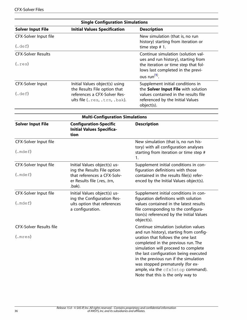
Single Configuration Simulations
DescriptionInitial Values SpecificationSolver Input File
New simulation (that is, no runhistory) starting from iteration ortime step # 1.
CFX-Solver Input file
(.def )
Continue simulation (solution val-ues and run history), starting from
CFX-Solver Results
(.res ) the iteration or time step that fol-lows last completed in the previ-
ous run[1].
Supplement initial conditions inthe Solver Input File with solution
Initial Values object(s) usingthe Results File option that
CFX-Solver Input
(.def ) values contained in the results filereferences a CFX-Solver Res-ults file (.res , .trn , .bak ). referenced by the Initial Values
object(s).
Multi-Configuration Simulations
DescriptionConfiguration-Specific
Initial Values Specifica-
tion
Solver Input File
New simulation (that is, no run his-tory) with all configuration analyses
CFX-Solver Input file
(.mdef ) starting from iteration or time step #1.
Supplement initial conditions in con-figuration definitions with those
Initial Values object(s) us-ing the Results File option
CFX-Solver Input file
(.mdef ) contained in the results file(s) refer-enced by the Initial Values object(s).
that references a CFX-Solv-er Results file (.res, .trn,.bak).
Supplement initial conditions in con-figuration definitions with solution
Initial Values object(s) us-ing the Configuration Res-
CFX-Solver Input file
(.mdef ) values contained in the latest resultsults option that referencesa configuration. file corresponding to the configura-
tion(s) referenced by the Initial Valuesobject(s).
Continue simulation (solution valuesand run history), starting from config-
CFX-Solver Results file
(.mres ) uration that follows the one lastcompleted in the previous run. Thesimulation will proceed to completethe last configuration being executedin the previous run if the simulationwas stopped prematurely (for ex-ample, via the cfx5stop command).Note that this is the only way to
Release 15.0 - © SAS IP, Inc. All rights reserved. - Contains proprietary and confidential informationof ANSYS, Inc. and its subsidiaries and affiliates.36
CFX-Solver Files
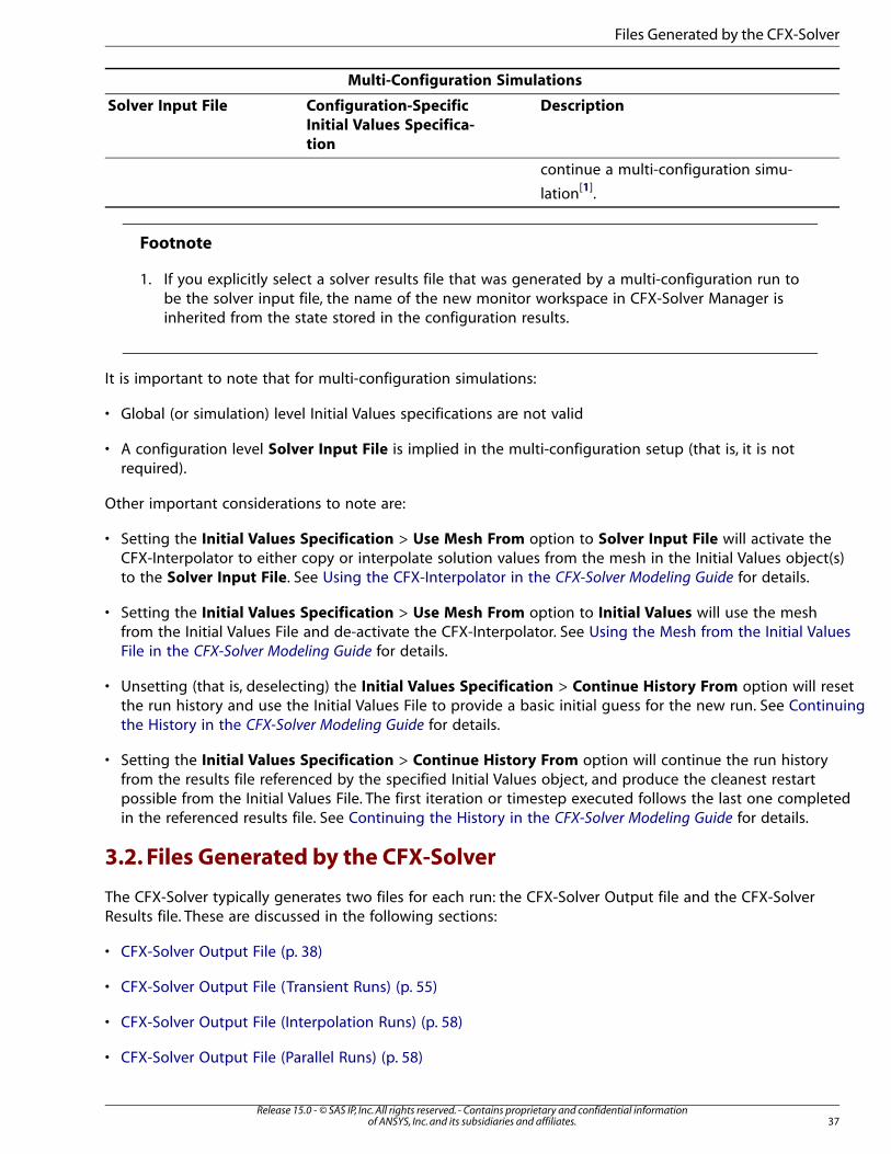
Multi-Configuration Simulations
DescriptionConfiguration-Specific
Initial Values Specifica-
tion
Solver Input File
continue a multi-configuration simu-
lation[1].
Footnote
1. If you explicitly select a solver results file that was generated by a multi-configuration run tobe the solver input file, the name of the new monitor workspace in CFX-Solver Manager isinherited from the state stored in the configuration results.
It is important to note that for multi-configuration simulations:
• Global (or simulation) level Initial Values specifications are not valid
• A configuration level Solver Input File is implied in the multi-configuration setup (that is, it is notrequired).
Other important considerations to note are:
• Setting the Initial Values Specification > Use Mesh From option to Solver Input File will activate theCFX-Interpolator to either copy or interpolate solution values from the mesh in the Initial Values object(s)to the Solver Input File. See Using the CFX-Interpolator in the CFX-Solver Modeling Guide for details.
• Setting the Initial Values Specification > Use Mesh From option to Initial Values will use the meshfrom the Initial Values File and de-activate the CFX-Interpolator. See Using the Mesh from the Initial ValuesFile in the CFX-Solver Modeling Guide for details.
• Unsetting (that is, deselecting) the Initial Values Specification > Continue History From option will resetthe run history and use the Initial Values File to provide a basic initial guess for the new run. See Continuingthe History in the CFX-Solver Modeling Guide for details.
• Setting the Initial Values Specification > Continue History From option will continue the run historyfrom the results file referenced by the specified Initial Values object, and produce the cleanest restartpossible from the Initial Values File. The first iteration or timestep executed follows the last one completedin the referenced results file. See Continuing the History in the CFX-Solver Modeling Guide for details.
3.2. Files Generated by the CFX-Solver
The CFX-Solver typically generates two files for each run: the CFX-Solver Output file and the CFX-SolverResults file. These are discussed in the following sections:
• CFX-Solver Output File (p. 38)
• CFX-Solver Output File (Transient Runs) (p. 55)
• CFX-Solver Output File (Interpolation Runs) (p. 58)
• CFX-Solver Output File (Parallel Runs) (p. 58)
37Release 15.0 - © SAS IP, Inc. All rights reserved. - Contains proprietary and confidential information
of ANSYS, Inc. and its subsidiaries and affiliates.
Files Generated by the CFX-Solver

• CFX-Solver Output File (Mesh Adaption Runs) (p. 61)
• CFX-Solver Output File (Remeshing Runs) (p. 62)
• CFX-Solver Output File (Conjugate Heat Transfer Runs) (p. 62)
• CFX-Solver Output File (GGI Runs) (p. 63)
• CFX-Solver Output File (Combustion Runs) (p. 64)
• CFX-Solver Output File (Particle Runs) (p. 66)
• CFX-Solver Output File (ANSYS Multi-field Runs) (p. 70)
• CFX-Solver Output File (Radiation Runs) (p. 71)
• CFX-Solver Output File (Rigid Body Runs) (p. 73)
• CFX-Solver Results File (p. 73)
Additional files are generated for the run as follows:
• For runs that involve the use of the Discrete Transfer or Monte Carlo radiation models, an additional filecontaining radiation data can also be generated. See CFX Radiation File (p. 75).
• For parallel runs of the CFX-Solver, an additional CFX partition file can also be generated. See CFX PartitionFile (p. 77).
• For ANSYS Multi-field runs, additional files are created. See Additional Files for ANSYS Multi-field Runs (p. 77).
For multi-configuration simulations, the CFX-Solver generates two additional simulation level text outputand results files in addition to the output and results files generated per configuration. These files arediscussed in the sections:
• CFX Multi-Configuration Output File (p. 77)
• CFX Multi-Configuration Results File (p. 82)
3.2.1. CFX-Solver Output File
The CFX-Solver Output file is a formatted text file generated by the CFX-Solver and contains informationabout your CFX model setup, the state of the solution during execution of the CFX-Solver, and analysisstatistics for the particular run. This is the same information written to the text output window of theCFX-Solver Manager. For details, see Text Output Window (p. 5).
The file is formatted and divided into sections to enable quick and easy interpretation. The sectionsthat are present for any calculation may depend upon which physical models are being used (that is,whether the model is transient or steady-state) and whether the CFX-Solver is being run as severalparallel processes or as a single process.
The CFX-Solver will generate an output file with a name based on the CFX-Solver input file. For example,running the CFX-Solver using the input file named file.def in a clean working directory will generatean output file named file_001.out .
Release 15.0 - © SAS IP, Inc. All rights reserved. - Contains proprietary and confidential informationof ANSYS, Inc. and its subsidiaries and affiliates.38
CFX-Solver Files
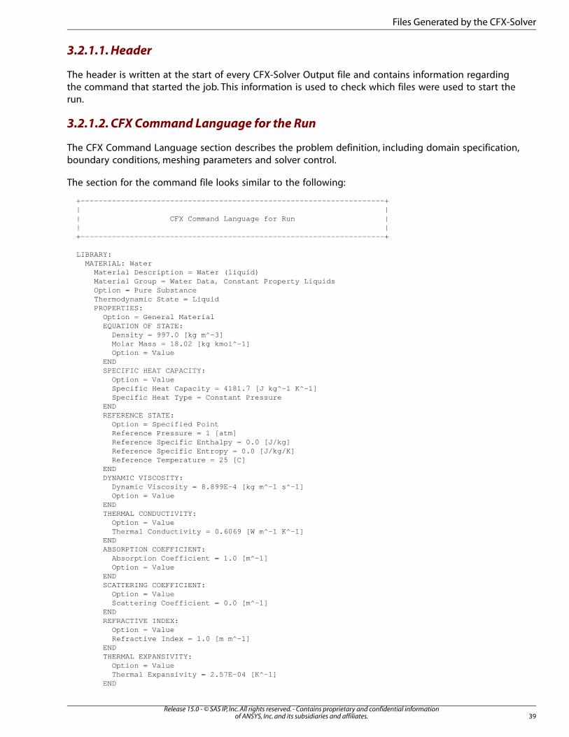
3.2.1.1. Header
The header is written at the start of every CFX-Solver Output file and contains information regardingthe command that started the job. This information is used to check which files were used to start therun.
3.2.1.2. CFX Command Language for the Run
The CFX Command Language section describes the problem definition, including domain specification,boundary conditions, meshing parameters and solver control.
The section for the command file looks similar to the following:
+--------------------------------------------------------------------+ | | | CFX Command Language for Run | | | +--------------------------------------------------------------------+
LIBRARY: MATERIAL: Water Material Description = Water (liquid) Material Group = Water Data, Constant Property Liquids Option = Pure Substance Thermodynamic State = Liquid PROPERTIES: Option = General Material EQUATION OF STATE: Density = 997.0 [kg m^-3] Molar Mass = 18.02 [kg kmol^-1] Option = Value END SPECIFIC HEAT CAPACITY: Option = Value Specific Heat Capacity = 4181.7 [J kg^-1 K^-1] Specific Heat Type = Constant Pressure END REFERENCE STATE: Option = Specified Point Reference Pressure = 1 [atm] Reference Specific Enthalpy = 0.0 [J/kg] Reference Specific Entropy = 0.0 [J/kg/K] Reference Temperature = 25 [C] END DYNAMIC VISCOSITY: Dynamic Viscosity = 8.899E-4 [kg m^-1 s^-1] Option = Value END THERMAL CONDUCTIVITY: Option = Value Thermal Conductivity = 0.6069 [W m^-1 K^-1] END ABSORPTION COEFFICIENT: Absorption Coefficient = 1.0 [m^-1] Option = Value END SCATTERING COEFFICIENT: Option = Value Scattering Coefficient = 0.0 [m^-1] END REFRACTIVE INDEX: Option = Value Refractive Index = 1.0 [m m^-1] END THERMAL EXPANSIVITY: Option = Value Thermal Expansivity = 2.57E-04 [K^-1] END
39Release 15.0 - © SAS IP, Inc. All rights reserved. - Contains proprietary and confidential information
of ANSYS, Inc. and its subsidiaries and affiliates.
Files Generated by the CFX-Solver
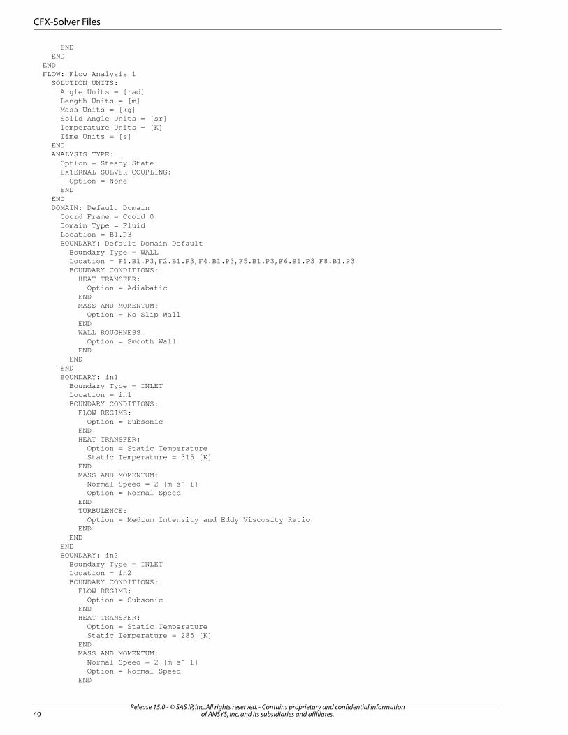
END END END FLOW: Flow Analysis 1 SOLUTION UNITS: Angle Units = [rad] Length Units = [m] Mass Units = [kg] Solid Angle Units = [sr] Temperature Units = [K] Time Units = [s] END ANALYSIS TYPE: Option = Steady State EXTERNAL SOLVER COUPLING: Option = None END END DOMAIN: Default Domain Coord Frame = Coord 0 Domain Type = Fluid Location = B1.P3 BOUNDARY: Default Domain Default Boundary Type = WALL Location = F1.B1.P3,F2.B1.P3,F4.B1.P3,F5.B1.P3,F6.B1.P3,F8.B1.P3 BOUNDARY CONDITIONS: HEAT TRANSFER: Option = Adiabatic END MASS AND MOMENTUM: Option = No Slip Wall END WALL ROUGHNESS: Option = Smooth Wall END END END BOUNDARY: in1 Boundary Type = INLET Location = in1 BOUNDARY CONDITIONS: FLOW REGIME: Option = Subsonic END HEAT TRANSFER: Option = Static Temperature Static Temperature = 315 [K] END MASS AND MOMENTUM: Normal Speed = 2 [m s^-1] Option = Normal Speed END TURBULENCE: Option = Medium Intensity and Eddy Viscosity Ratio END END END BOUNDARY: in2 Boundary Type = INLET Location = in2 BOUNDARY CONDITIONS: FLOW REGIME: Option = Subsonic END HEAT TRANSFER: Option = Static Temperature Static Temperature = 285 [K] END MASS AND MOMENTUM: Normal Speed = 2 [m s^-1] Option = Normal Speed END
Release 15.0 - © SAS IP, Inc. All rights reserved. - Contains proprietary and confidential informationof ANSYS, Inc. and its subsidiaries and affiliates.40
CFX-Solver Files
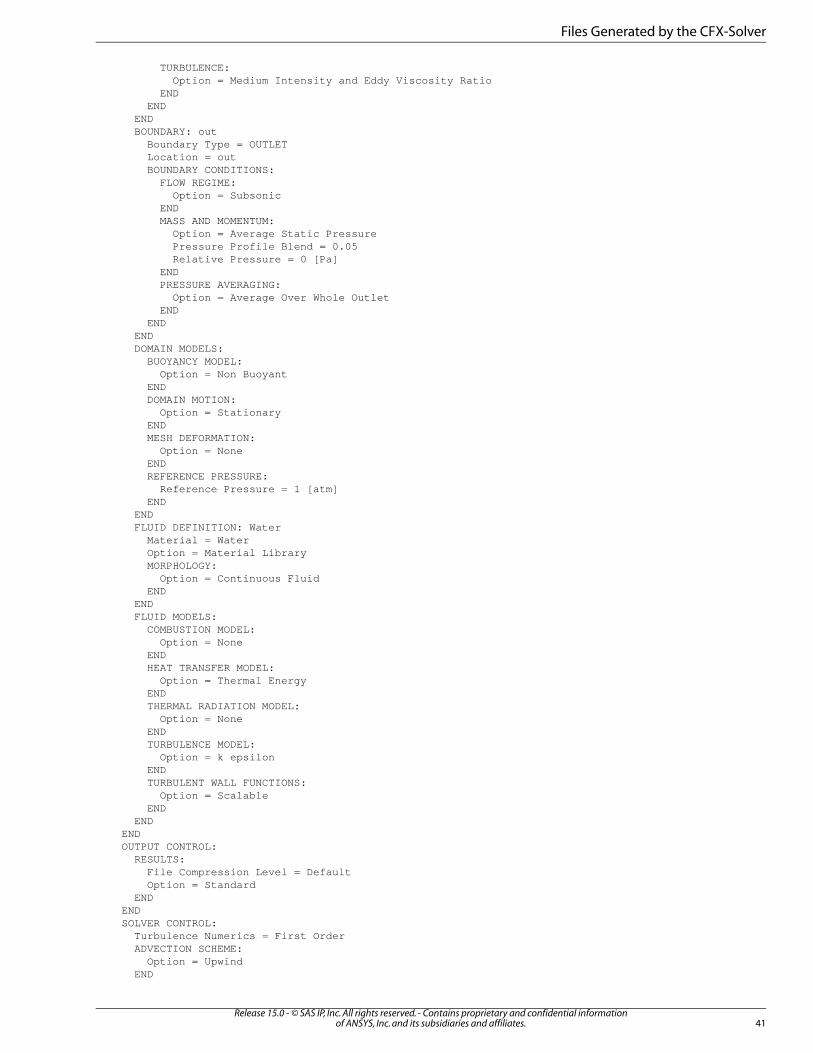
TURBULENCE: Option = Medium Intensity and Eddy Viscosity Ratio END END END BOUNDARY: out Boundary Type = OUTLET Location = out BOUNDARY CONDITIONS: FLOW REGIME: Option = Subsonic END MASS AND MOMENTUM: Option = Average Static Pressure Pressure Profile Blend = 0.05 Relative Pressure = 0 [Pa] END PRESSURE AVERAGING: Option = Average Over Whole Outlet END END END DOMAIN MODELS: BUOYANCY MODEL: Option = Non Buoyant END DOMAIN MOTION: Option = Stationary END MESH DEFORMATION: Option = None END REFERENCE PRESSURE: Reference Pressure = 1 [atm] END END FLUID DEFINITION: Water Material = Water Option = Material Library MORPHOLOGY: Option = Continuous Fluid END END FLUID MODELS: COMBUSTION MODEL: Option = None END HEAT TRANSFER MODEL: Option = Thermal Energy END THERMAL RADIATION MODEL: Option = None END TURBULENCE MODEL: Option = k epsilon END TURBULENT WALL FUNCTIONS: Option = Scalable END END END OUTPUT CONTROL: RESULTS: File Compression Level = Default Option = Standard END END SOLVER CONTROL: Turbulence Numerics = First Order ADVECTION SCHEME: Option = Upwind END
41Release 15.0 - © SAS IP, Inc. All rights reserved. - Contains proprietary and confidential information
of ANSYS, Inc. and its subsidiaries and affiliates.
Files Generated by the CFX-Solver
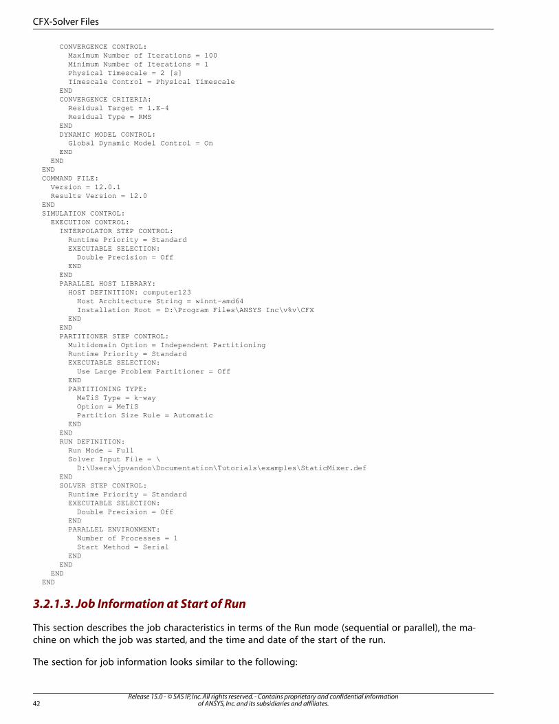
CONVERGENCE CONTROL: Maximum Number of Iterations = 100 Minimum Number of Iterations = 1 Physical Timescale = 2 [s] Timescale Control = Physical Timescale END CONVERGENCE CRITERIA: Residual Target = 1.E-4 Residual Type = RMS END DYNAMIC MODEL CONTROL: Global Dynamic Model Control = On END END END COMMAND FILE: Version = 12.0.1 Results Version = 12.0 END SIMULATION CONTROL: EXECUTION CONTROL: INTERPOLATOR STEP CONTROL: Runtime Priority = Standard EXECUTABLE SELECTION: Double Precision = Off END END PARALLEL HOST LIBRARY: HOST DEFINITION: computer123 Host Architecture String = winnt-amd64 Installation Root = D:\Program Files\ANSYS Inc\v%v\CFX END END PARTITIONER STEP CONTROL: Multidomain Option = Independent Partitioning Runtime Priority = Standard EXECUTABLE SELECTION: Use Large Problem Partitioner = Off END PARTITIONING TYPE: MeTiS Type = k-way Option = MeTiS Partition Size Rule = Automatic END END RUN DEFINITION: Run Mode = Full Solver Input File = \ D:\Users\jpvandoo\Documentation\Tutorials\examples\StaticMixer.def END SOLVER STEP CONTROL: Runtime Priority = Standard EXECUTABLE SELECTION: Double Precision = Off END PARALLEL ENVIRONMENT: Number of Processes = 1 Start Method = Serial END END END END
3.2.1.3. Job Information at Start of Run
This section describes the job characteristics in terms of the Run mode (sequential or parallel), the ma-chine on which the job was started, and the time and date of the start of the run.
The section for job information looks similar to the following:
Release 15.0 - © SAS IP, Inc. All rights reserved. - Contains proprietary and confidential informationof ANSYS, Inc. and its subsidiaries and affiliates.42
CFX-Solver Files
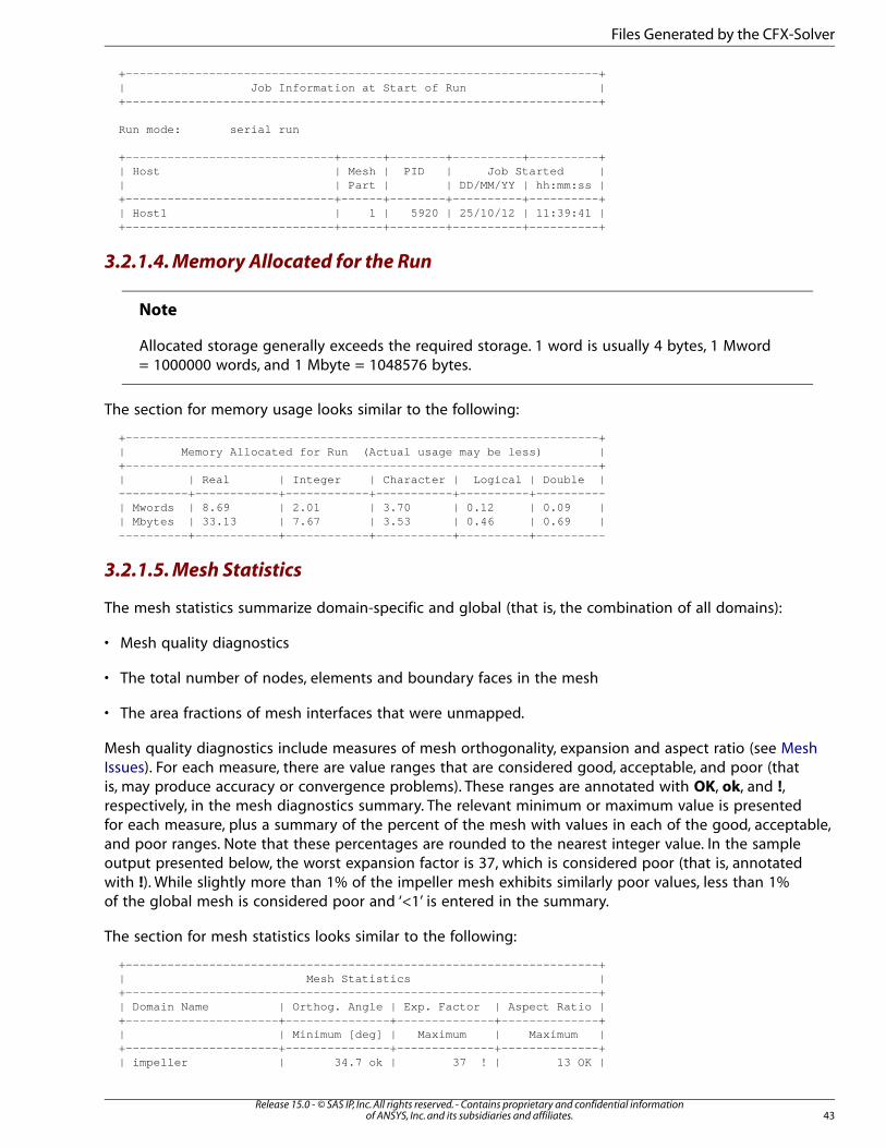
+--------------------------------------------------------------------+ | Job Information at Start of Run | +--------------------------------------------------------------------+
Run mode: serial run
+------------------------------+------+--------+----------+----------+ | Host | Mesh | PID | Job Started | | | Part | | DD/MM/YY | hh:mm:ss | +------------------------------+------+--------+----------+----------+ | Host1 | 1 | 5920 | 25/10/12 | 11:39:41 | +------------------------------+------+--------+----------+----------+
3.2.1.4. Memory Allocated for the Run
Note
Allocated storage generally exceeds the required storage. 1 word is usually 4 bytes, 1 Mword= 1000000 words, and 1 Mbyte = 1048576 bytes.
The section for memory usage looks similar to the following:
+--------------------------------------------------------------------+ | Memory Allocated for Run (Actual usage may be less) | +--------------------------------------------------------------------+ | | Real | Integer | Character | Logical | Double | ----------+------------+------------+-----------+----------+---------- | Mwords | 8.69 | 2.01 | 3.70 | 0.12 | 0.09 | | Mbytes | 33.13 | 7.67 | 3.53 | 0.46 | 0.69 | ----------+------------+------------+-----------+----------+----------
3.2.1.5. Mesh Statistics
The mesh statistics summarize domain-specific and global (that is, the combination of all domains):
• Mesh quality diagnostics
• The total number of nodes, elements and boundary faces in the mesh
• The area fractions of mesh interfaces that were unmapped.
Mesh quality diagnostics include measures of mesh orthogonality, expansion and aspect ratio (see MeshIssues). For each measure, there are value ranges that are considered good, acceptable, and poor (thatis, may produce accuracy or convergence problems). These ranges are annotated with OK, ok, and !,respectively, in the mesh diagnostics summary. The relevant minimum or maximum value is presentedfor each measure, plus a summary of the percent of the mesh with values in each of the good, acceptable,and poor ranges. Note that these percentages are rounded to the nearest integer value. In the sampleoutput presented below, the worst expansion factor is 37, which is considered poor (that is, annotatedwith !). While slightly more than 1% of the impeller mesh exhibits similarly poor values, less than 1%of the global mesh is considered poor and ‘<1’ is entered in the summary.
The section for mesh statistics looks similar to the following:
+--------------------------------------------------------------------+ | Mesh Statistics | +--------------------------------------------------------------------+ | Domain Name | Orthog. Angle | Exp. Factor | Aspect Ratio | +----------------------+---------------+--------------+--------------+ | | Minimum [deg] | Maximum | Maximum | +----------------------+---------------+--------------+--------------+ | impeller | 34.7 ok | 37 ! | 13 OK |
43Release 15.0 - © SAS IP, Inc. All rights reserved. - Contains proprietary and confidential information
of ANSYS, Inc. and its subsidiaries and affiliates.
Files Generated by the CFX-Solver
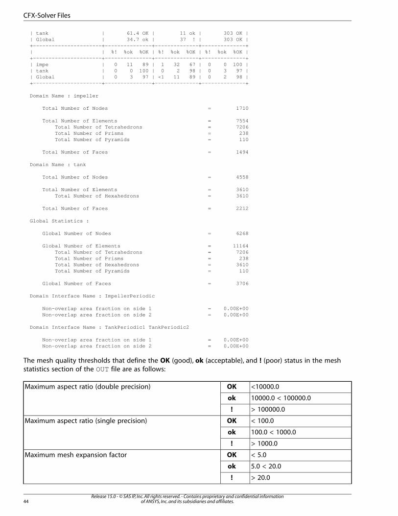
| tank | 61.4 OK | 11 ok | 303 OK | | Global | 34.7 ok | 37 ! | 303 OK | +----------------------+---------------+--------------+--------------+ | | %! %ok %OK | %! %ok %OK | %! %ok %OK | +----------------------+---------------+--------------+--------------+ | impe | 0 11 89 | 1 32 67 | 0 0 100 | | tank | 0 0 100 | 0 2 98 | 0 3 97 | | Global | 0 3 97 | <1 11 89 | 0 2 98 | +----------------------+---------------+--------------+--------------+
Domain Name : impeller
Total Number of Nodes = 1710
Total Number of Elements = 7554 Total Number of Tetrahedrons = 7206 Total Number of Prisms = 238 Total Number of Pyramids = 110
Total Number of Faces = 1494
Domain Name : tank
Total Number of Nodes = 4558
Total Number of Elements = 3610 Total Number of Hexahedrons = 3610
Total Number of Faces = 2212
Global Statistics :
Global Number of Nodes = 6268
Global Number of Elements = 11164 Total Number of Tetrahedrons = 7206 Total Number of Prisms = 238 Total Number of Hexahedrons = 3610 Total Number of Pyramids = 110
Global Number of Faces = 3706
Domain Interface Name : ImpellerPeriodic
Non-overlap area fraction on side 1 = 0.00E+00 Non-overlap area fraction on side 2 = 0.00E+00
Domain Interface Name : TankPeriodic1 TankPeriodic2
Non-overlap area fraction on side 1 = 0.00E+00 Non-overlap area fraction on side 2 = 0.00E+00
The mesh quality thresholds that define the OK (good), ok (acceptable), and ! (poor) status in the meshstatistics section of the OUT file are as follows:
<10000.0OKMaximum aspect ratio (double precision)
10000.0 < 100000.0ok
> 100000.0!
< 100.0OKMaximum aspect ratio (single precision)
100.0 < 1000.0ok
> 1000.0!
< 5.0OKMaximum mesh expansion factor
5.0 < 20.0ok
> 20.0!
Release 15.0 - © SAS IP, Inc. All rights reserved. - Contains proprietary and confidential informationof ANSYS, Inc. and its subsidiaries and affiliates.44
CFX-Solver Files
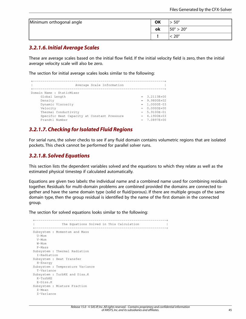
> 50°OKMinimum orthogonal angle
50° > 20°ok
< 20°!
3.2.1.6. Initial Average Scales
These are average scales based on the initial flow field. If the initial velocity field is zero, then the initialaverage velocity scale will also be zero.
The section for initial average scales looks similar to the following:
+--------------------------------------------------------------------+| Average Scale Information |+--------------------------------------------------------------------+Domain Name : StaticMixer Global Length = 3.2113E+00 Density = 9.9800E+02 Dynamic Viscosity = 1.0000E-03 Velocity = 0.0000E+00 Thermal Conductivity = 5.9100E-01 Specific Heat Capacity at Constant Pressure = 4.1900E+03 Prandtl Number = 7.0897E+00
3.2.1.7. Checking for Isolated Fluid Regions
For serial runs, the solver checks to see if any fluid domain contains volumetric regions that are isolatedpockets. This check cannot be performed for parallel solver runs.
3.2.1.8. Solved Equations
This section lists the dependent variables solved and the equations to which they relate as well as theestimated physical timestep if calculated automatically.
Equations are given two labels: the individual name and a combined name used for combining residualstogether. Residuals for multi-domain problems are combined provided the domains are connected to-gether and have the same domain type (solid or fluid/porous). If there are multiple groups of the samedomain type, then the group residual is identified by the name of the first domain in the connectedgroup.
The section for solved equations looks similar to the following:
+--------------------------------------------------------------------+ | The Equations Solved in This Calculation | +--------------------------------------------------------------------+ Subsystem : Momentum and Mass U-Mom V-Mom W-Mom P-Mass Subsystem : Thermal Radiation I-Radiation Subsystem : Heat Transfer H-Energy Subsystem : Temperature Variance T-Variance Subsystem : TurbKE and Diss.K K-TurbKE E-Diss.K Subsystem : Mixture Fraction Z-Mean Z-Variance
45Release 15.0 - © SAS IP, Inc. All rights reserved. - Contains proprietary and confidential information
of ANSYS, Inc. and its subsidiaries and affiliates.
Files Generated by the CFX-Solver
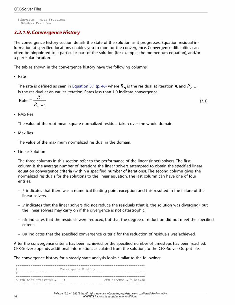
Subsystem : Mass Fractions NO-Mass Fraction
3.2.1.9. Convergence History
The convergence history section details the state of the solution as it progresses. Equation residual in-formation at specified locations enables you to monitor the convergence. Convergence difficulties canoften be pinpointed to a particular part of the solution (for example, the momentum equation), and/ora particular location.
The tables shown in the convergence history have the following columns:
• Rate
The rate is defined as seen in Equation 3.1 (p. 46) where �� is the residual at iteration �, and −�� �
is the residual at an earlier iteration. Rates less than 1.0 indicate convergence.
(3.1)=−
�
�
�
� �
• RMS Res
The value of the root mean square normalized residual taken over the whole domain.
• Max Res
The value of the maximum normalized residual in the domain.
• Linear Solution
The three columns in this section refer to the performance of the linear (inner) solvers. The firstcolumn is the average number of iterations the linear solvers attempted to obtain the specified linearequation convergence criteria (within a specified number of iterations). The second column gives thenormalized residuals for the solutions to the linear equation. The last column can have one of fourentries:
– * indicates that there was a numerical floating point exception and this resulted in the failure of thelinear solvers.
– F indicates that the linear solvers did not reduce the residuals (that is, the solution was diverging), butthe linear solvers may carry on if the divergence is not catastrophic.
– ok indicates that the residuals were reduced, but that the degree of reduction did not meet the specifiedcriteria.
– OK indicates that the specified convergence criteria for the reduction of residuals was achieved.
After the convergence criteria has been achieved, or the specified number of timesteps has been reached,CFX-Solver appends additional information, calculated from the solution, to the CFX-Solver Output file.
The convergence history for a steady state analysis looks similar to the following:
+--------------------------------------------------------------------+| Convergence History |+--------------------------------------------------------------------+======================================================================OUTER LOOP ITERATION = 1 CPU SECONDS = 2.68E+00----------------------------------------------------------------------
Release 15.0 - © SAS IP, Inc. All rights reserved. - Contains proprietary and confidential informationof ANSYS, Inc. and its subsidiaries and affiliates.46
CFX-Solver Files
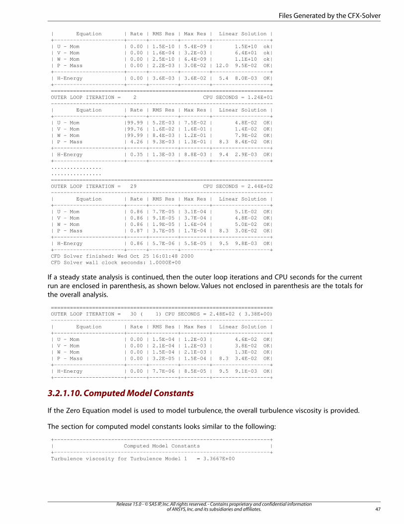
| Equation | Rate | RMS Res | Max Res | Linear Solution |+----------------------+------+---------+---------+------------------+| U - Mom | 0.00 | 1.5E-10 | 5.4E-09 | 1.5E+10 ok|| V - Mom | 0.00 | 1.6E-04 | 3.2E-03 | 6.4E+01 ok|| W - Mom | 0.00 | 2.5E-10 | 6.4E-09 | 1.1E+10 ok|| P - Mass | 0.00 | 2.2E-03 | 3.0E-02 | 12.0 9.5E-02 OK|+----------------------+------+---------+---------+------------------+| H-Energy | 0.00 | 3.6E-03 | 3.6E-02 | 5.4 8.0E-03 OK|+----------------------+------+---------+---------+------------------+======================================================================OUTER LOOP ITERATION = 2 CPU SECONDS = 1.24E+01----------------------------------------------------------------------| Equation | Rate | RMS Res | Max Res | Linear Solution |+----------------------+------+---------+---------+------------------+| U - Mom |99.99 | 5.2E-03 | 7.5E-02 | 4.8E-02 OK|| V - Mom |99.76 | 1.6E-02 | 1.6E-01 | 1.4E-02 OK|| W - Mom |99.99 | 8.4E-03 | 1.2E-01 | 7.9E-02 OK|| P - Mass | 4.26 | 9.3E-03 | 1.3E-01 | 8.3 8.4E-02 OK|+----------------------+------+---------+---------+------------------+| H-Energy | 0.35 | 1.3E-03 | 8.8E-03 | 9.4 2.9E-03 OK|+----------------------+------+---------+---------+------------------+................................======================================================================OUTER LOOP ITERATION = 29 CPU SECONDS = 2.44E+02----------------------------------------------------------------------| Equation | Rate | RMS Res | Max Res | Linear Solution |+----------------------+------+---------+---------+------------------+| U - Mom | 0.86 | 7.7E-05 | 3.1E-04 | 5.1E-02 OK|| V - Mom | 0.86 | 9.1E-05 | 3.7E-04 | 4.8E-02 OK|| W - Mom | 0.86 | 1.9E-05 | 1.6E-04 | 5.0E-02 OK|| P - Mass | 0.87 | 3.7E-05 | 1.7E-04 | 8.3 3.0E-02 OK|+----------------------+------+---------+---------+------------------+| H-Energy | 0.86 | 5.7E-06 | 5.5E-05 | 9.5 9.8E-03 OK|+----------------------+------+---------+---------+------------------+CFD Solver finished: Wed Oct 25 16:01:48 2000CFD Solver wall clock seconds: 1.0000E+00
If a steady state analysis is continued, then the outer loop iterations and CPU seconds for the currentrun are enclosed in parenthesis, as shown below. Values not enclosed in parenthesis are the totals forthe overall analysis.
======================================================================OUTER LOOP ITERATION = 30 ( 1) CPU SECONDS = 2.48E+02 ( 3.38E+00)----------------------------------------------------------------------| Equation | Rate | RMS Res | Max Res | Linear Solution |+----------------------+------+---------+---------+------------------+| U - Mom | 0.00 | 1.5E-04 | 1.2E-03 | 4.6E-02 OK|| V - Mom | 0.00 | 2.1E-04 | 1.2E-03 | 3.8E-02 OK|| W - Mom | 0.00 | 1.5E-04 | 2.1E-03 | 1.3E-02 OK|| P - Mass | 0.00 | 3.2E-05 | 1.5E-04 | 8.3 3.4E-02 OK|+----------------------+------+---------+---------+------------------+| H-Energy | 0.00 | 7.7E-06 | 8.5E-05 | 9.5 9.1E-03 OK|+----------------------+------+---------+---------+------------------+
3.2.1.10. Computed Model Constants
If the Zero Equation model is used to model turbulence, the overall turbulence viscosity is provided.
The section for computed model constants looks similar to the following:
+--------------------------------------------------------------------+| Computed Model Constants |+--------------------------------------------------------------------+Turbulence viscosity for Turbulence Model 1 = 3.3667E+00
47Release 15.0 - © SAS IP, Inc. All rights reserved. - Contains proprietary and confidential information
of ANSYS, Inc. and its subsidiaries and affiliates.
Files Generated by the CFX-Solver
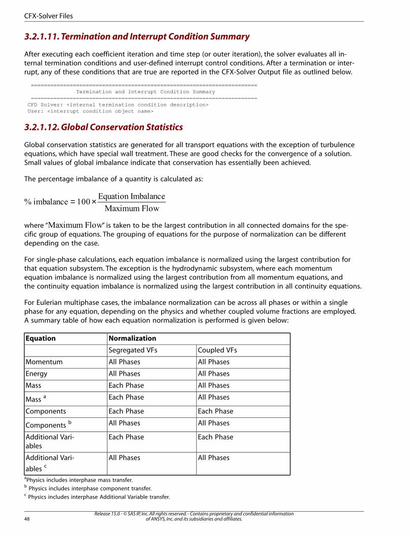
3.2.1.11. Termination and Interrupt Condition Summary
After executing each coefficient iteration and time step (or outer iteration), the solver evaluates all in-ternal termination conditions and user-defined interrupt control conditions. After a termination or inter-rupt, any of these conditions that are true are reported in the CFX-Solver Output file as outlined below.
====================================================================== Termination and Interrupt Condition Summary ======================================================================CFD Solver: <internal termination condition description> User: <interrupt condition object name>
3.2.1.12. Global Conservation Statistics
Global conservation statistics are generated for all transport equations with the exception of turbulenceequations, which have special wall treatment. These are good checks for the convergence of a solution.Small values of global imbalance indicate that conservation has essentially been achieved.
The percentage imbalance of a quantity is calculated as:
= ×
where “ ” is taken to be the largest contribution in all connected domains for the spe-cific group of equations. The grouping of equations for the purpose of normalization can be differentdepending on the case.
For single-phase calculations, each equation imbalance is normalized using the largest contribution forthat equation subsystem. The exception is the hydrodynamic subsystem, where each momentumequation imbalance is normalized using the largest contribution from all momentum equations, andthe continuity equation imbalance is normalized using the largest contribution in all continuity equations.
For Eulerian multiphase cases, the imbalance normalization can be across all phases or within a singlephase for any equation, depending on the physics and whether coupled volume fractions are employed.A summary table of how each equation normalization is performed is given below:
NormalizationEquation
Coupled VFsSegregated VFs
All PhasesAll PhasesMomentum
All PhasesAll PhasesEnergy
All PhasesEach PhaseMass
All PhasesEach PhaseMass a
Each PhaseEach PhaseComponents
All PhasesAll PhasesComponents b
Each PhaseEach PhaseAdditional Vari-ables
All PhasesAll PhasesAdditional Vari-
ables c
aPhysics includes interphase mass transfer.b Physics includes interphase component transfer.c Physics includes interphase Additional Variable transfer.
Release 15.0 - © SAS IP, Inc. All rights reserved. - Contains proprietary and confidential informationof ANSYS, Inc. and its subsidiaries and affiliates.48
CFX-Solver Files

The section for global conservation statistics looks similar to the following:
====================================================================== Boundary Flow and Total Source Term Summary ======================================================================
+--------------------------------------------------------------------+ | U-Mom | +--------------------------------------------------------------------+ Boundary : CatConv Default -9.4754E-01 Boundary : Inlet 1.6971E+00 Boundary : InletSide Side 1 1.3262E-05 Boundary : Outlet -1.0523E+00 Boundary : OutletSide Side 1 -1.7085E-07 Sub-Domain : catalyst 2.6129E-01 Neg Accumulation : CatConv 4.1436E-02 Domain Interface : InletSide (Side 1) -1.1166E-02 Domain Interface : InletSide (Side 2) 1.1166E-02 Domain Interface : OutletSide (Side 1) -1.4308E-05 Domain Interface : OutletSide (Side 2) 1.4308E-05 ----------- Domain Imbalance : -3.6059E-05
Domain Imbalance, in %: -0.0002 %
+--------------------------------------------------------------------+ | V-Mom | +--------------------------------------------------------------------+ Boundary : CatConv Default -3.3355E-02 Boundary : Inlet 1.1009E-07 Boundary : InletSide Side 1 7.2564E-06 Boundary : Outlet -4.7561E-04 Boundary : OutletSide Side 1 1.9734E-08 Sub-Domain : catalyst 3.4056E-02 Neg Accumulation : CatConv -2.4319E-04 Domain Interface : InletSide (Side 1) -4.7260E-04 Domain Interface : InletSide (Side 2) 4.7262E-04 Domain Interface : OutletSide (Side 1) 7.5672E-06 Domain Interface : OutletSide (Side 2) -7.5672E-06 ----------- Domain Imbalance : -1.0275E-05
Domain Imbalance, in %: 0.0000 %
+--------------------------------------------------------------------+ | W-Mom | +--------------------------------------------------------------------+ Boundary : CatConv Default -1.1450E+01 Boundary : Inlet -1.6971E+00 Boundary : InletSide Side 1 1.3180E-01 Boundary : Outlet 1.0628E+00 Boundary : OutletSide Side 1 -6.8369E-02 Sub-Domain : catalyst 1.2137E+01 Neg Accumulation : CatConv -1.8195E-01 Domain Interface : InletSide (Side 1) 2.2715E+01 Domain Interface : InletSide (Side 2) -2.2592E+01 Domain Interface : OutletSide (Side 1) -1.0548E+01 Domain Interface : OutletSide (Side 2) 1.0493E+01 ----------- Domain Imbalance : 1.4353E-03
Domain Imbalance, in %: 0.0063 %
+--------------------------------------------------------------------+ | P-Mass | +--------------------------------------------------------------------+ Boundary : Inlet 2.8382E-02 Boundary : Outlet -5.6938E-02 Neg Accumulation : CatConv 2.8576E-02 Domain Interface : InletSide (Side 1) -3.0665E-02 Domain Interface : InletSide (Side 2) 3.0665E-02 Domain Interface : OutletSide (Side 1) 5.6543E-02
49Release 15.0 - © SAS IP, Inc. All rights reserved. - Contains proprietary and confidential information
of ANSYS, Inc. and its subsidiaries and affiliates.
Files Generated by the CFX-Solver
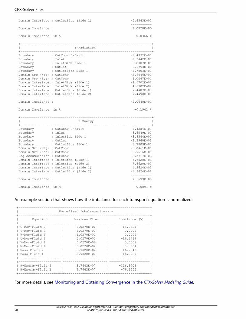
Domain Interface : OutletSide (Side 2) -5.6543E-02 ----------- Domain Imbalance : 2.0828E-05
Domain Imbalance, in %: 0.0366 %
+--------------------------------------------------------------------+ | I-Radiation | +--------------------------------------------------------------------+ Boundary : CatConv Default -1.4392E+01 Boundary : Inlet 1.9442E+01 Boundary : InletSide Side 1 3.8307E-01 Boundary : Outlet -6.1793E+00 Boundary : OutletSide Side 1 -1.7803E-01 Domain Src (Neg) : CatConv -2.9646E-01 Domain Src (Pos) : CatConv 3.0447E-01 Domain Interface : InletSide (Side 1) -4.6702E+02 Domain Interface : InletSide (Side 2) 4.6702E+02 Domain Interface : OutletSide (Side 1) -7.4487E+01 Domain Interface : OutletSide (Side 2) 7.4490E+01 ----------- Domain Imbalance : -9.0640E-01
Domain Imbalance, in %: -0.1941 %
+--------------------------------------------------------------------+ | H-Energy | +--------------------------------------------------------------------+ Boundary : CatConv Default 1.4284E+01 Boundary : Inlet 8.6049E+03 Boundary : InletSide Side 1 -3.8344E-01 Boundary : Outlet -2.3960E+02 Boundary : OutletSide Side 1 1.7809E-01 Domain Src (Neg) : CatConv -3.0461E-01 Domain Src (Pos) : CatConv 2.9616E-01 Neg Accumulation : CatConv -8.3717E+03 Domain Interface : InletSide (Side 1) -7.6620E+03 Domain Interface : InletSide (Side 2) 7.6620E+03 Domain Interface : OutletSide (Side 1) 1.3624E+02 Domain Interface : OutletSide (Side 2) -1.3624E+02 ----------- Domain Imbalance : 7.6699E+00
Domain Imbalance, in %: 0.0891 %
An example section that shows how the imbalance for each transport equation is normalized:
+--------------------------------------------------------------------+| Normalised Imbalance Summary |+--------------------------------------------------------------------+| Equation | Maximum Flow | Imbalance (%) |+--------------------------------------------------------------------+| U-Mom-Fluid 2 | 6.0270E+02 | 15.9327 || V-Mom-Fluid 2 | 6.0270E+02 | 0.0000 || W-Mom-Fluid 2 | 6.0270E+02 | 0.0004 || U-Mom-Fluid 1 | 6.0270E+02 | -16.6732 || V-Mom-Fluid 1 | 6.0270E+02 | 0.0001 || W-Mom-Fluid 1 | 6.0270E+02 | 0.0004 || Mass-Fluid 2 | 5.9820E+02 | 16.2942 || Mass-Fluid 1 | 5.9820E+02 | -16.2929 |+----------------------+-----------------------+---------------------++----------------------+-----------------------+---------------------+| H-Energy-Fluid 2 | 3.7642E+07 | -136.9703 || H-Energy-Fluid 1 | 3.7642E+07 | -76.2664 |+----------------------+-----------------------+---------------------+
For more details, see Monitoring and Obtaining Convergence in the CFX-Solver Modeling Guide.
Release 15.0 - © SAS IP, Inc. All rights reserved. - Contains proprietary and confidential informationof ANSYS, Inc. and its subsidiaries and affiliates.50
CFX-Solver Files
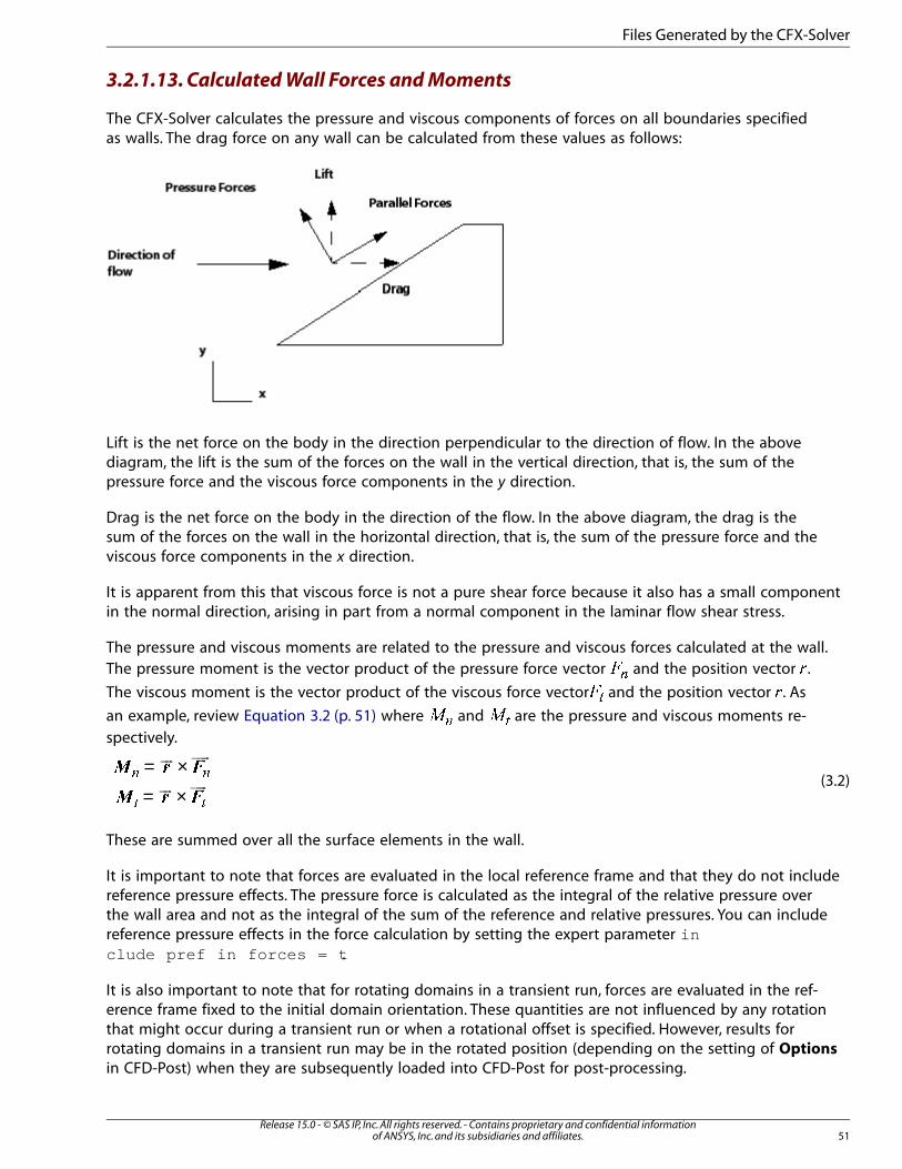
3.2.1.13. Calculated Wall Forces and Moments
The CFX-Solver calculates the pressure and viscous components of forces on all boundaries specifiedas walls. The drag force on any wall can be calculated from these values as follows:
Lift is the net force on the body in the direction perpendicular to the direction of flow. In the abovediagram, the lift is the sum of the forces on the wall in the vertical direction, that is, the sum of thepressure force and the viscous force components in the y direction.
Drag is the net force on the body in the direction of the flow. In the above diagram, the drag is thesum of the forces on the wall in the horizontal direction, that is, the sum of the pressure force and theviscous force components in the x direction.
It is apparent from this that viscous force is not a pure shear force because it also has a small componentin the normal direction, arising in part from a normal component in the laminar flow shear stress.
The pressure and viscous moments are related to the pressure and viscous forces calculated at the wall.
The pressure moment is the vector product of the pressure force vector �� and the position vector �.
The viscous moment is the vector product of the viscous force vector�� and the position vector �. As
an example, review Equation 3.2 (p. 51) where �� and � are the pressure and viscous moments re-
spectively.
(3.2)= ×= ×
� �
� �
� �
ururu
ur
uru
These are summed over all the surface elements in the wall.
It is important to note that forces are evaluated in the local reference frame and that they do not includereference pressure effects. The pressure force is calculated as the integral of the relative pressure overthe wall area and not as the integral of the sum of the reference and relative pressures. You can includereference pressure effects in the force calculation by setting the expert parameter include pref in forces = t .
It is also important to note that for rotating domains in a transient run, forces are evaluated in the ref-erence frame fixed to the initial domain orientation. These quantities are not influenced by any rotationthat might occur during a transient run or when a rotational offset is specified. However, results forrotating domains in a transient run may be in the rotated position (depending on the setting of Options
in CFD-Post) when they are subsequently loaded into CFD-Post for post-processing.
51Release 15.0 - © SAS IP, Inc. All rights reserved. - Contains proprietary and confidential information
of ANSYS, Inc. and its subsidiaries and affiliates.
Files Generated by the CFX-Solver
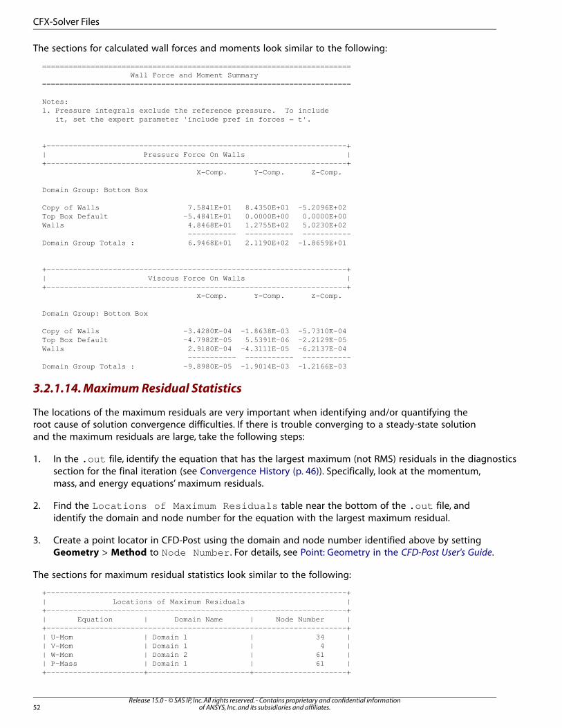
The sections for calculated wall forces and moments look similar to the following:
====================================================================== Wall Force and Moment Summary ======================================================================
Notes: 1. Pressure integrals exclude the reference pressure. To include it, set the expert parameter 'include pref in forces = t'.
+--------------------------------------------------------------------+ | Pressure Force On Walls | +--------------------------------------------------------------------+ X-Comp. Y-Comp. Z-Comp.
Domain Group: Bottom Box
Copy of Walls 7.5841E+01 8.4350E+01 -5.2096E+02 Top Box Default -5.4841E+01 0.0000E+00 0.0000E+00 Walls 4.8468E+01 1.2755E+02 5.0230E+02 ----------- ----------- ----------- Domain Group Totals : 6.9468E+01 2.1190E+02 -1.8659E+01
+--------------------------------------------------------------------+ | Viscous Force On Walls | +--------------------------------------------------------------------+ X-Comp. Y-Comp. Z-Comp.
Domain Group: Bottom Box
Copy of Walls -3.4280E-04 -1.8638E-03 -5.7310E-04 Top Box Default -4.7982E-05 5.5391E-06 -2.2129E-05 Walls 2.9180E-04 -4.3111E-05 -6.2137E-04 ----------- ----------- ----------- Domain Group Totals : -9.8980E-05 -1.9014E-03 -1.2166E-03
3.2.1.14. Maximum Residual Statistics
The locations of the maximum residuals are very important when identifying and/or quantifying theroot cause of solution convergence difficulties. If there is trouble converging to a steady-state solutionand the maximum residuals are large, take the following steps:
1. In the .out file, identify the equation that has the largest maximum (not RMS) residuals in the diagnosticssection for the final iteration (see Convergence History (p. 46)). Specifically, look at the momentum,mass, and energy equations’ maximum residuals.
2. Find the Locations of Maximum Residuals table near the bottom of the .out file, andidentify the domain and node number for the equation with the largest maximum residual.
3. Create a point locator in CFD-Post using the domain and node number identified above by settingGeometry > Method to Node Number . For details, see Point: Geometry in the CFD-Post User's Guide.
The sections for maximum residual statistics look similar to the following:
+--------------------------------------------------------------------+ | Locations of Maximum Residuals | +--------------------------------------------------------------------+ | Equation | Domain Name | Node Number | +--------------------------------------------------------------------+ | U-Mom | Domain 1 | 34 | | V-Mom | Domain 1 | 4 | | W-Mom | Domain 2 | 61 | | P-Mass | Domain 1 | 61 | +----------------------+-----------------------+---------------------+
Release 15.0 - © SAS IP, Inc. All rights reserved. - Contains proprietary and confidential informationof ANSYS, Inc. and its subsidiaries and affiliates.52
CFX-Solver Files
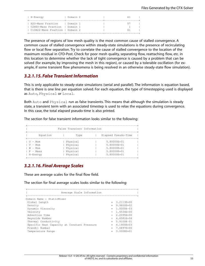
| H-Energy | Domain 2 | 61 | +----------------------+-----------------------+---------------------+ | H2O-Mass Fraction | Domain 1 | 57 | | C2H6O-Mass Fraction | Domain 1 | 1 | | C10H22-Mass Fraction | Domain 2 | 61 | +----------------------+-----------------------+---------------------+
The presence of regions of low mesh quality is the most common cause of stalled convergence. Acommon cause of stalled convergence within steady-state simulations is the presence of recirculatingflow or local flow separation. Try to correlate the cause of stalled convergence to the location of themaximum residual in CFD-Post. Check for poor mesh quality, separating flow, reattaching flow, etc. inthis location to determine whether the lack of tight convergence is caused by a problem that can besolved (for example, by improving the mesh in this region), or caused by a tolerable oscillation (for ex-ample, if some transient flow phenomena is being resolved in an otherwise steady-state flow simulation).
3.2.1.15. False Transient Information
This is only applicable to steady-state simulations (serial and parallel). The information is equation based,that is there is one line per equation solved. For each equation, the type of timestepping used is displayedas Auto , Physical or Local .
Both Auto and Physical run as false transients. This means that although the simulation is steadystate, a transient term with an associated timestep is used to relax the equations during convergence.In this case, the total elapsed pseudo-time is also printed.
The section for false transient information looks similar to the following:
+--------------------------------------------------------------------+| False Transient Information |+--------------------------------------------------------------------+| Equation | Type | Elapsed Pseudo-Time |+--------------------------------------------------------------------+| U - Mom | Physical | 5.80000E+01 || V - Mom | Physical | 5.80000E+01 || W - Mom | Physical | 5.80000E+01 || P - Mass | Physical | 5.80000E+01 || H-Energy | Physical | 5.80000E+01 |+--------------------------------------------------------------------+
3.2.1.16. Final Average Scales
These are average scales for the final flow field.
The section for final average scales looks similar to the following:
+--------------------------------------------------------------------+| Average Scale Information |+--------------------------------------------------------------------+Domain Name : StaticMixer Global Length = 3.2113E+00 Density = 9.9800E+02 Dynamic Viscosity = 1.0000E-03 Velocity = 1.4534E+00 Advection Time = 2.2095E+00 Reynolds Number = 4.6581E+06 Thermal Conductivity = 5.9100E-01 Specific Heat Capacity at Constant Pressure = 4.1900E+03 Prandtl Number = 7.0897E+00 Temperature Range = 3.0008E+01
53Release 15.0 - © SAS IP, Inc. All rights reserved. - Contains proprietary and confidential information
of ANSYS, Inc. and its subsidiaries and affiliates.
Files Generated by the CFX-Solver
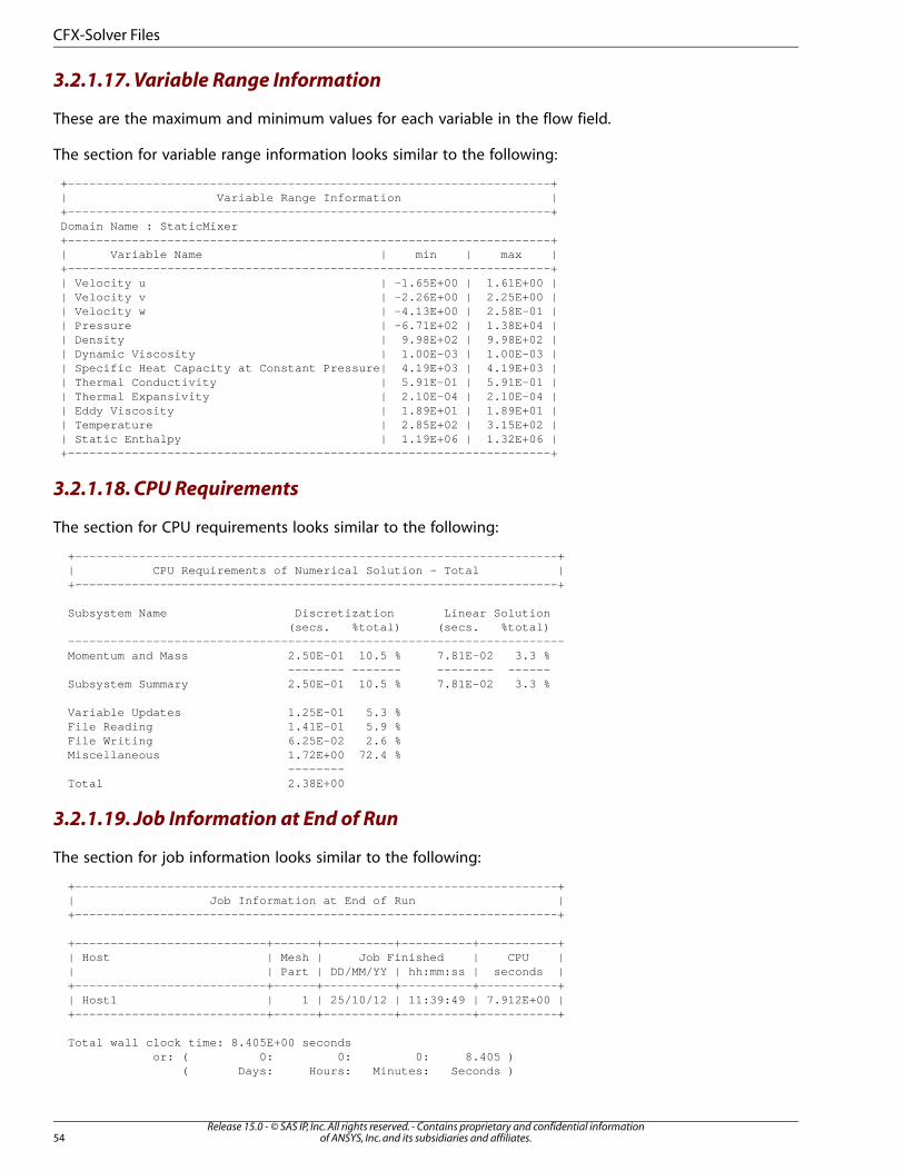
3.2.1.17. Variable Range Information
These are the maximum and minimum values for each variable in the flow field.
The section for variable range information looks similar to the following:
+--------------------------------------------------------------------+| Variable Range Information |+--------------------------------------------------------------------+Domain Name : StaticMixer+--------------------------------------------------------------------+| Variable Name | min | max |+--------------------------------------------------------------------+| Velocity u | -1.65E+00 | 1.61E+00 || Velocity v | -2.26E+00 | 2.25E+00 || Velocity w | -4.13E+00 | 2.58E-01 || Pressure | -6.71E+02 | 1.38E+04 || Density | 9.98E+02 | 9.98E+02 || Dynamic Viscosity | 1.00E-03 | 1.00E-03 || Specific Heat Capacity at Constant Pressure| 4.19E+03 | 4.19E+03 || Thermal Conductivity | 5.91E-01 | 5.91E-01 || Thermal Expansivity | 2.10E-04 | 2.10E-04 || Eddy Viscosity | 1.89E+01 | 1.89E+01 || Temperature | 2.85E+02 | 3.15E+02 || Static Enthalpy | 1.19E+06 | 1.32E+06 |+--------------------------------------------------------------------+
3.2.1.18. CPU Requirements
The section for CPU requirements looks similar to the following:
+--------------------------------------------------------------------+ | CPU Requirements of Numerical Solution - Total | +--------------------------------------------------------------------+
Subsystem Name Discretization Linear Solution (secs. %total) (secs. %total) ---------------------------------------------------------------------- Momentum and Mass 2.50E-01 10.5 % 7.81E-02 3.3 % -------- ------- -------- ------ Subsystem Summary 2.50E-01 10.5 % 7.81E-02 3.3 %
Variable Updates 1.25E-01 5.3 % File Reading 1.41E-01 5.9 % File Writing 6.25E-02 2.6 % Miscellaneous 1.72E+00 72.4 % -------- Total 2.38E+00
3.2.1.19. Job Information at End of Run
The section for job information looks similar to the following:
+--------------------------------------------------------------------+ | Job Information at End of Run | +--------------------------------------------------------------------+
+---------------------------+------+----------+----------+-----------+ | Host | Mesh | Job Finished | CPU | | | Part | DD/MM/YY | hh:mm:ss | seconds | +---------------------------+------+----------+----------+-----------+ | Host1 | 1 | 25/10/12 | 11:39:49 | 7.912E+00 | +---------------------------+------+----------+----------+-----------+
Total wall clock time: 8.405E+00 seconds or: ( 0: 0: 0: 8.405 ) ( Days: Hours: Minutes: Seconds )
Release 15.0 - © SAS IP, Inc. All rights reserved. - Contains proprietary and confidential informationof ANSYS, Inc. and its subsidiaries and affiliates.54
CFX-Solver Files
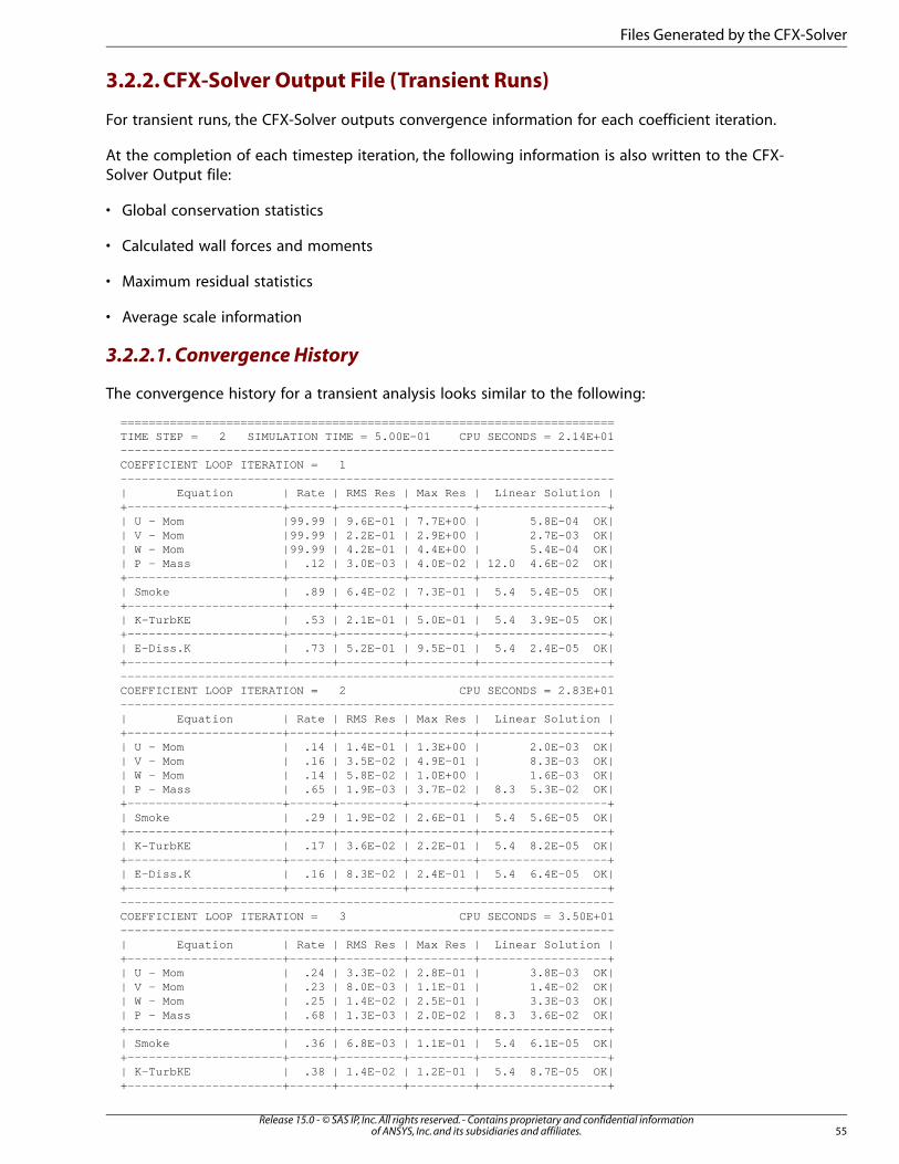
3.2.2. CFX-Solver Output File (Transient Runs)
For transient runs, the CFX-Solver outputs convergence information for each coefficient iteration.
At the completion of each timestep iteration, the following information is also written to the CFX-Solver Output file:
• Global conservation statistics
• Calculated wall forces and moments
• Maximum residual statistics
• Average scale information
3.2.2.1. Convergence History
The convergence history for a transient analysis looks similar to the following:
====================================================================== TIME STEP = 2 SIMULATION TIME = 5.00E-01 CPU SECONDS = 2.14E+01 ---------------------------------------------------------------------- COEFFICIENT LOOP ITERATION = 1 ---------------------------------------------------------------------- | Equation | Rate | RMS Res | Max Res | Linear Solution | +----------------------+------+---------+---------+------------------+ | U - Mom |99.99 | 9.6E-01 | 7.7E+00 | 5.8E-04 OK| | V - Mom |99.99 | 2.2E-01 | 2.9E+00 | 2.7E-03 OK| | W - Mom |99.99 | 4.2E-01 | 4.4E+00 | 5.4E-04 OK| | P - Mass | .12 | 3.0E-03 | 4.0E-02 | 12.0 4.6E-02 OK| +----------------------+------+---------+---------+------------------+ | Smoke | .89 | 6.4E-02 | 7.3E-01 | 5.4 5.4E-05 OK| +----------------------+------+---------+---------+------------------+ | K-TurbKE | .53 | 2.1E-01 | 5.0E-01 | 5.4 3.9E-05 OK| +----------------------+------+---------+---------+------------------+ | E-Diss.K | .73 | 5.2E-01 | 9.5E-01 | 5.4 2.4E-05 OK| +----------------------+------+---------+---------+------------------+ ---------------------------------------------------------------------- COEFFICIENT LOOP ITERATION = 2 CPU SECONDS = 2.83E+01 ---------------------------------------------------------------------- | Equation | Rate | RMS Res | Max Res | Linear Solution | +----------------------+------+---------+---------+------------------+ | U - Mom | .14 | 1.4E-01 | 1.3E+00 | 2.0E-03 OK| | V - Mom | .16 | 3.5E-02 | 4.9E-01 | 8.3E-03 OK| | W - Mom | .14 | 5.8E-02 | 1.0E+00 | 1.6E-03 OK| | P - Mass | .65 | 1.9E-03 | 3.7E-02 | 8.3 5.3E-02 OK| +----------------------+------+---------+---------+------------------+ | Smoke | .29 | 1.9E-02 | 2.6E-01 | 5.4 5.6E-05 OK| +----------------------+------+---------+---------+------------------+ | K-TurbKE | .17 | 3.6E-02 | 2.2E-01 | 5.4 8.2E-05 OK| +----------------------+------+---------+---------+------------------+ | E-Diss.K | .16 | 8.3E-02 | 2.4E-01 | 5.4 6.4E-05 OK| +----------------------+------+---------+---------+------------------+ ---------------------------------------------------------------------- COEFFICIENT LOOP ITERATION = 3 CPU SECONDS = 3.50E+01 ---------------------------------------------------------------------- | Equation | Rate | RMS Res | Max Res | Linear Solution | +----------------------+------+---------+---------+------------------+ | U - Mom | .24 | 3.3E-02 | 2.8E-01 | 3.8E-03 OK| | V - Mom | .23 | 8.0E-03 | 1.1E-01 | 1.4E-02 OK| | W - Mom | .25 | 1.4E-02 | 2.5E-01 | 3.3E-03 OK| | P - Mass | .68 | 1.3E-03 | 2.0E-02 | 8.3 3.6E-02 OK| +----------------------+------+---------+---------+------------------+ | Smoke | .36 | 6.8E-03 | 1.1E-01 | 5.4 6.1E-05 OK| +----------------------+------+---------+---------+------------------+ | K-TurbKE | .38 | 1.4E-02 | 1.2E-01 | 5.4 8.7E-05 OK| +----------------------+------+---------+---------+------------------+
55Release 15.0 - © SAS IP, Inc. All rights reserved. - Contains proprietary and confidential information
of ANSYS, Inc. and its subsidiaries and affiliates.
Files Generated by the CFX-Solver
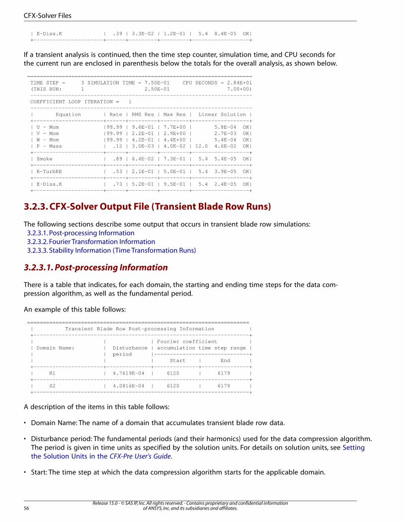
| E-Diss.K | .39 | 3.3E-02 | 1.2E-01 | 5.4 8.4E-05 OK| +----------------------+------+---------+---------+------------------+
If a transient analysis is continued, then the time step counter, simulation time, and CPU seconds forthe current run are enclosed in parenthesis below the totals for the overall analysis, as shown below.
======================================================================= TIME STEP = 3 SIMULATION TIME = 7.50E-01 CPU SECONDS = 2.84E+01 (THIS RUN: 1 2.50E-01 7.00+00) ---------------------------------------------------------------------- COEFFICIENT LOOP ITERATION = 1 ---------------------------------------------------------------------- | Equation | Rate | RMS Res | Max Res | Linear Solution | +----------------------+------+---------+---------+------------------+ | U - Mom |99.99 | 9.6E-01 | 7.7E+00 | 5.8E-04 OK| | V - Mom |99.99 | 2.2E-01 | 2.9E+00 | 2.7E-03 OK| | W - Mom |99.99 | 4.2E-01 | 4.4E+00 | 5.4E-04 OK| | P - Mass | .12 | 3.0E-03 | 4.0E-02 | 12.0 4.6E-02 OK| +----------------------+------+---------+---------+------------------+ | Smoke | .89 | 6.4E-02 | 7.3E-01 | 5.4 5.4E-05 OK| +----------------------+------+---------+---------+------------------+ | K-TurbKE | .53 | 2.1E-01 | 5.0E-01 | 5.4 3.9E-05 OK| +----------------------+------+---------+---------+------------------+ | E-Diss.K | .73 | 5.2E-01 | 9.5E-01 | 5.4 2.4E-05 OK| +----------------------+------+---------+---------+------------------+
3.2.3. CFX-Solver Output File (Transient Blade Row Runs)
The following sections describe some output that occurs in transient blade row simulations:3.2.3.1. Post-processing Information3.2.3.2. Fourier Transformation Information3.2.3.3. Stability Information (Time Transformation Runs)
3.2.3.1. Post-processing Information
There is a table that indicates, for each domain, the starting and ending time steps for the data com-pression algorithm, as well as the fundamental period.
An example of this table follows:
====================================================================== | Transient Blade Row Post-processing Information | +--------------------------------------------------------------------+ | | | Fourier coefficient | | Domain Name: | Disturbance | accumulation time step range | | | period |------------------------------+ | | | Start | End | +----------------------+--------------+--------------+---------------+ | R1 | 4.7619E-04 | 6120 | 6179 | +--------------------------------------------------------------------+ | S2 | 4.0816E-04 | 6120 | 6179 | +--------------------------------------------------------------------+
A description of the items in this table follows:
• Domain Name: The name of a domain that accumulates transient blade row data.
• Disturbance period: The fundamental periods (and their harmonics) used for the data compression algorithm.The period is given in time units as specified by the solution units. For details on solution units, see Settingthe Solution Units in the CFX-Pre User's Guide.
• Start: The time step at which the data compression algorithm starts for the applicable domain.
Release 15.0 - © SAS IP, Inc. All rights reserved. - Contains proprietary and confidential informationof ANSYS, Inc. and its subsidiaries and affiliates.56
CFX-Solver Files
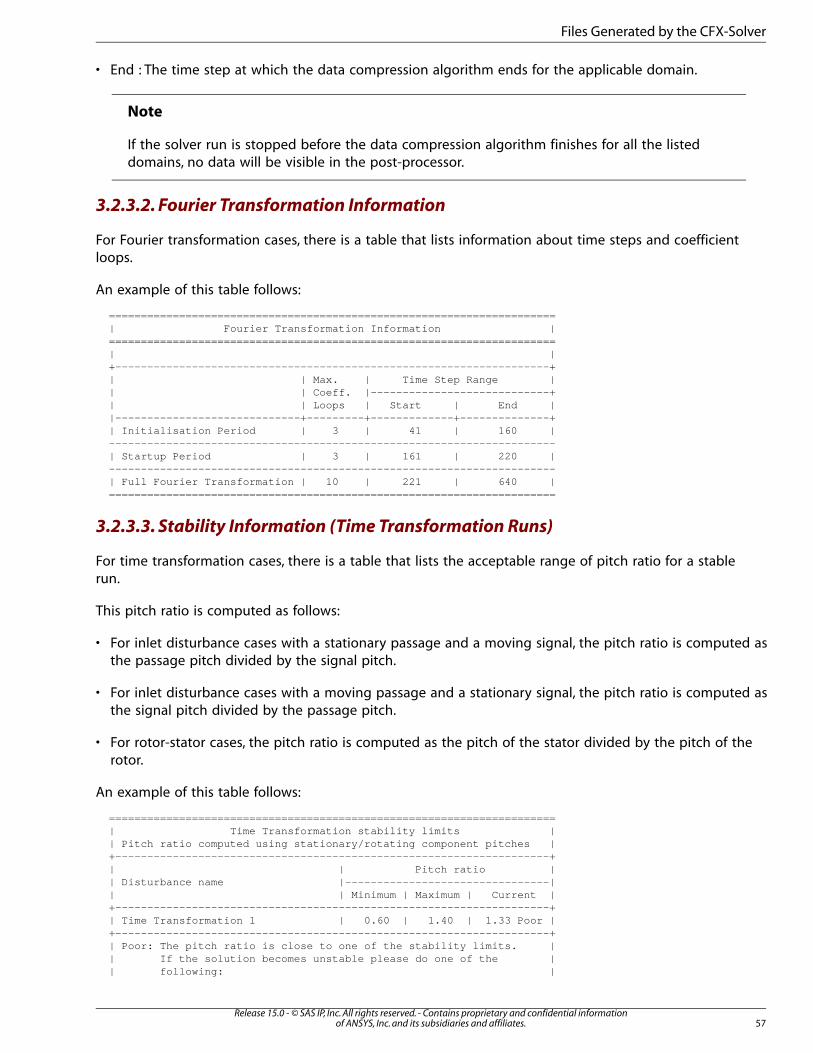
• End : The time step at which the data compression algorithm ends for the applicable domain.
Note
If the solver run is stopped before the data compression algorithm finishes for all the listeddomains, no data will be visible in the post-processor.
3.2.3.2. Fourier Transformation Information
For Fourier transformation cases, there is a table that lists information about time steps and coefficientloops.
An example of this table follows:
====================================================================== | Fourier Transformation Information | ====================================================================== | | +--------------------------------------------------------------------+ | | Max. | Time Step Range | | | Coeff. |----------------------------+ | | Loops | Start | End | |-----------------------------+---------+-------------+--------------+ | Initialisation Period | 3 | 41 | 160 | ---------------------------------------------------------------------- | Startup Period | 3 | 161 | 220 | ---------------------------------------------------------------------- | Full Fourier Transformation | 10 | 221 | 640 | ======================================================================
3.2.3.3. Stability Information (Time Transformation Runs)
For time transformation cases, there is a table that lists the acceptable range of pitch ratio for a stablerun.
This pitch ratio is computed as follows:
• For inlet disturbance cases with a stationary passage and a moving signal, the pitch ratio is computed asthe passage pitch divided by the signal pitch.
• For inlet disturbance cases with a moving passage and a stationary signal, the pitch ratio is computed asthe signal pitch divided by the passage pitch.
• For rotor-stator cases, the pitch ratio is computed as the pitch of the stator divided by the pitch of therotor.
An example of this table follows:
====================================================================== | Time Transformation stability limits | | Pitch ratio computed using stationary/rotating component pitches | +--------------------------------------------------------------------+ | | Pitch ratio | | Disturbance name |--------------------------------| | | Minimum | Maximum | Current | +--------------------------------------------------------------------+ | Time Transformation 1 | 0.60 | 1.40 | 1.33 Poor | +--------------------------------------------------------------------+ | Poor: The pitch ratio is close to one of the stability limits. | | If the solution becomes unstable please do one of the | | following: |
57Release 15.0 - © SAS IP, Inc. All rights reserved. - Contains proprietary and confidential information
of ANSYS, Inc. and its subsidiaries and affiliates.
Files Generated by the CFX-Solver
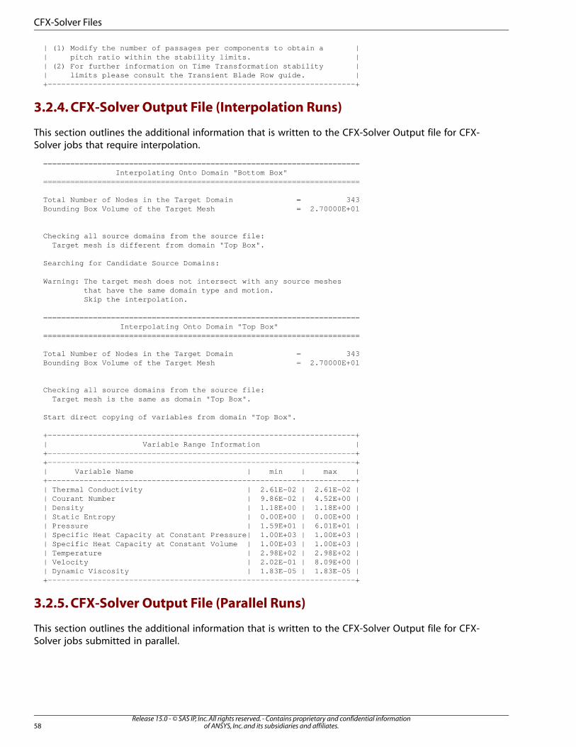
| (1) Modify the number of passages per components to obtain a | | pitch ratio within the stability limits. | | (2) For further information on Time Transformation stability | | limits please consult the Transient Blade Row guide. | +--------------------------------------------------------------------+
3.2.4. CFX-Solver Output File (Interpolation Runs)
This section outlines the additional information that is written to the CFX-Solver Output file for CFX-Solver jobs that require interpolation.
====================================================================== Interpolating Onto Domain "Bottom Box" ======================================================================
Total Number of Nodes in the Target Domain = 343 Bounding Box Volume of the Target Mesh = 2.70000E+01
Checking all source domains from the source file: Target mesh is different from domain "Top Box".
Searching for Candidate Source Domains:
Warning: The target mesh does not intersect with any source meshes that have the same domain type and motion. Skip the interpolation.
====================================================================== Interpolating Onto Domain "Top Box" ======================================================================
Total Number of Nodes in the Target Domain = 343 Bounding Box Volume of the Target Mesh = 2.70000E+01
Checking all source domains from the source file: Target mesh is the same as domain "Top Box".
Start direct copying of variables from domain "Top Box".
+--------------------------------------------------------------------+ | Variable Range Information | +--------------------------------------------------------------------+ +--------------------------------------------------------------------+ | Variable Name | min | max | +--------------------------------------------------------------------+ | Thermal Conductivity | 2.61E-02 | 2.61E-02 | | Courant Number | 9.86E-02 | 4.52E+00 | | Density | 1.18E+00 | 1.18E+00 | | Static Entropy | 0.00E+00 | 0.00E+00 | | Pressure | 1.59E+01 | 6.01E+01 | | Specific Heat Capacity at Constant Pressure| 1.00E+03 | 1.00E+03 | | Specific Heat Capacity at Constant Volume | 1.00E+03 | 1.00E+03 | | Temperature | 2.98E+02 | 2.98E+02 | | Velocity | 2.02E-01 | 8.09E+00 | | Dynamic Viscosity | 1.83E-05 | 1.83E-05 | +--------------------------------------------------------------------+
3.2.5. CFX-Solver Output File (Parallel Runs)
This section outlines the additional information that is written to the CFX-Solver Output file for CFX-Solver jobs submitted in parallel.
Release 15.0 - © SAS IP, Inc. All rights reserved. - Contains proprietary and confidential informationof ANSYS, Inc. and its subsidiaries and affiliates.58
CFX-Solver Files
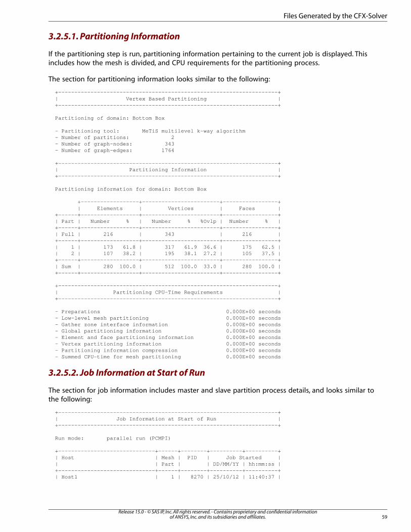
3.2.5.1. Partitioning Information
If the partitioning step is run, partitioning information pertaining to the current job is displayed. Thisincludes how the mesh is divided, and CPU requirements for the partitioning process.
The section for partitioning information looks similar to the following:
+--------------------------------------------------------------------+ | Vertex Based Partitioning | +--------------------------------------------------------------------+
Partitioning of domain: Bottom Box
- Partitioning tool: MeTiS multilevel k-way algorithm - Number of partitions: 2 - Number of graph-nodes: 343 - Number of graph-edges: 1764
+--------------------------------------------------------------------+ | Partitioning Information | +--------------------------------------------------------------------+
Partitioning information for domain: Bottom Box
+------------------+------------------------+-----------------+ | Elements | Vertices | Faces | +------+------------------+------------------------+-----------------+ | Part | Number % | Number % %Ovlp | Number % | +------+------------------+------------------------+-----------------+ | Full | 216 | 343 | 216 | +------+------------------+------------------------+-----------------+ | 1 | 173 61.8 | 317 61.9 36.6 | 175 62.5 | | 2 | 107 38.2 | 195 38.1 27.2 | 105 37.5 | +------+------------------+------------------------+-----------------+ | Sum | 280 100.0 | 512 100.0 33.0 | 280 100.0 | +------+------------------+------------------------+-----------------+
+--------------------------------------------------------------------+ | Partitioning CPU-Time Requirements | +--------------------------------------------------------------------+
- Preparations 0.000E+00 seconds - Low-level mesh partitioning 0.000E+00 seconds - Gather zone interface information 0.000E+00 seconds - Global partitioning information 0.000E+00 seconds - Element and face partitioning information 0.000E+00 seconds - Vertex partitioning information 0.000E+00 seconds - Partitioning information compression 0.000E+00 seconds - Summed CPU-time for mesh partitioning 0.000E+00 seconds
3.2.5.2. Job Information at Start of Run
The section for job information includes master and slave partition process details, and looks similar tothe following:
+--------------------------------------------------------------------+ | Job Information at Start of Run | +--------------------------------------------------------------------+
Run mode: parallel run (PCMPI)
+------------------------------+------+--------+----------+----------+ | Host | Mesh | PID | Job Started | | | Part | | DD/MM/YY | hh:mm:ss | +------------------------------+------+--------+----------+----------+ | Host1 | 1 | 8270 | 25/10/12 | 11:40:37 |
59Release 15.0 - © SAS IP, Inc. All rights reserved. - Contains proprietary and confidential information
of ANSYS, Inc. and its subsidiaries and affiliates.
Files Generated by the CFX-Solver
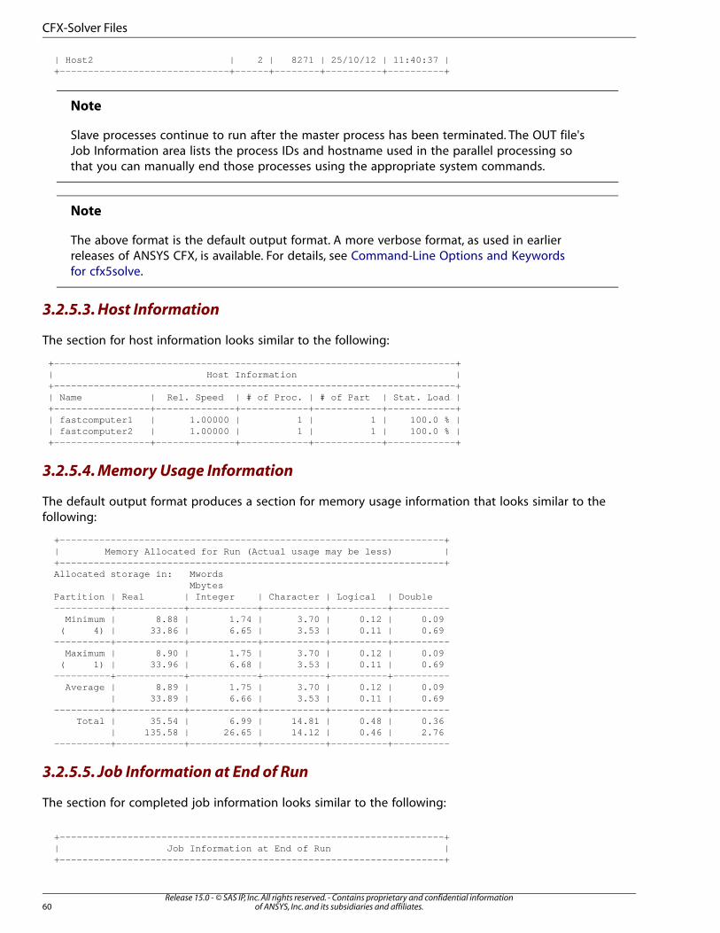
| Host2 | 2 | 8271 | 25/10/12 | 11:40:37 | +------------------------------+------+--------+----------+----------+
Note
Slave processes continue to run after the master process has been terminated. The OUT file'sJob Information area lists the process IDs and hostname used in the parallel processing sothat you can manually end those processes using the appropriate system commands.
Note
The above format is the default output format. A more verbose format, as used in earlierreleases of ANSYS CFX, is available. For details, see Command-Line Options and Keywordsfor cfx5solve.
3.2.5.3. Host Information
The section for host information looks similar to the following:
+-----------------------------------------------------------------------+| Host Information |+-----------------------------------------------------------------------+| Name | Rel. Speed | # of Proc. | # of Part | Stat. Load |+-----------------+--------------+------------+------------+------------+| fastcomputer1 | 1.00000 | 1 | 1 | 100.0 % || fastcomputer2 | 1.00000 | 1 | 1 | 100.0 % |+-----------------+--------------+------------+------------+------------+
3.2.5.4. Memory Usage Information
The default output format produces a section for memory usage information that looks similar to thefollowing:
+--------------------------------------------------------------------+ | Memory Allocated for Run (Actual usage may be less) | +--------------------------------------------------------------------+ Allocated storage in: Mwords Mbytes Partition | Real | Integer | Character | Logical | Double ----------+------------+------------+-----------+----------+---------- Minimum | 8.88 | 1.74 | 3.70 | 0.12 | 0.09 ( 4) | 33.86 | 6.65 | 3.53 | 0.11 | 0.69 ----------+------------+------------+-----------+----------+---------- Maximum | 8.90 | 1.75 | 3.70 | 0.12 | 0.09 ( 1) | 33.96 | 6.68 | 3.53 | 0.11 | 0.69 ----------+------------+------------+-----------+----------+---------- Average | 8.89 | 1.75 | 3.70 | 0.12 | 0.09 | 33.89 | 6.66 | 3.53 | 0.11 | 0.69 ----------+------------+------------+-----------+----------+---------- Total | 35.54 | 6.99 | 14.81 | 0.48 | 0.36 | 135.58 | 26.65 | 14.12 | 0.46 | 2.76 ----------+------------+------------+-----------+----------+----------
3.2.5.5. Job Information at End of Run
The section for completed job information looks similar to the following:
+--------------------------------------------------------------------+ | Job Information at End of Run | +--------------------------------------------------------------------+
Release 15.0 - © SAS IP, Inc. All rights reserved. - Contains proprietary and confidential informationof ANSYS, Inc. and its subsidiaries and affiliates.60
CFX-Solver Files
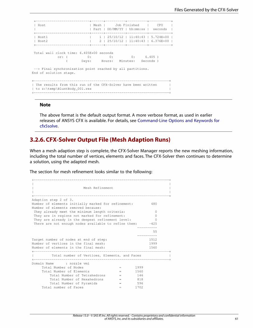
+---------------------------+------+----------+----------+-----------+ | Host | Mesh | Job Finished | CPU | | | Part | DD/MM/YY | hh:mm:ss | seconds | +---------------------------+------+----------+----------+-----------+ | Host1 | 1 | 25/10/12 | 11:40:43 | 5.724E+00 | | Host2 | 2 | 25/10/12 | 11:40:43 | 6.376E+00 | +---------------------------+------+----------+----------+-----------+
Total wall clock time: 6.405E+00 seconds or: ( 0: 0: 0: 6.405 ) ( Days: Hours: Minutes: Seconds )
--> Final synchronization point reached by all partitions.End of solution stage.
+--------------------------------------------------------------------+| The results from this run of the CFX-Solver have been written || to z:\temp\BluntBody_001.res |+--------------------------------------------------------------------+
Note
The above format is the default output format. A more verbose format, as used in earlierreleases of ANSYS CFX is available. For details, see Command-Line Options and Keywords forcfx5solve.
3.2.6. CFX-Solver Output File (Mesh Adaption Runs)
When a mesh adaption step is complete, the CFX-Solver Manager reports the new meshing information,including the total number of vertices, elements and faces. The CFX-Solver then continues to determinea solution, using the adapted mesh.
The section for mesh refinement looks similar to the following:
+--------------------------------------------------------------------+| || Mesh Refinement || |+--------------------------------------------------------------------+Adaption step 2 of 3.Number of elements initially marked for refinement: 480Number of elements removed because: They already meet the minimum length criteria: 0 They are in regions not marked for refinement: 0 They are already in the deepest refinement level: 0 There are not enough nodes available to refine them: -425 ---------- 55 ----------Target number of nodes at end of step: 1512Number of vertices in the final mesh: 1999Number of elements in the final mesh: 1560+--------------------------------------------------------------------+| Total number of Vertices, Elements, and Faces |+--------------------------------------------------------------------+Domain Name : nozzle vmi Total Number of Nodes = 1999 Total Number of Elements = 1560 Total Number of Tetrahedrons = 146 Total Number of Hexahedrons = 818 Total Number of Pyramids = 596 Total number of Faces = 1702
61Release 15.0 - © SAS IP, Inc. All rights reserved. - Contains proprietary and confidential information
of ANSYS, Inc. and its subsidiaries and affiliates.
Files Generated by the CFX-Solver
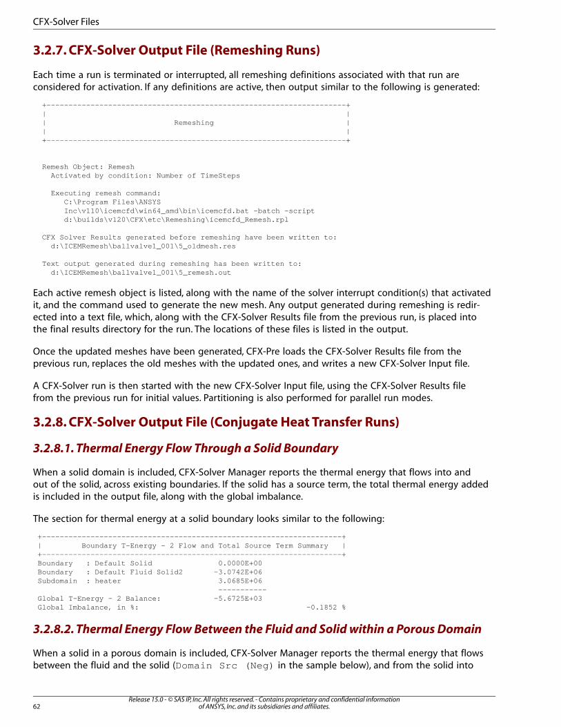
3.2.7. CFX-Solver Output File (Remeshing Runs)
Each time a run is terminated or interrupted, all remeshing definitions associated with that run areconsidered for activation. If any definitions are active, then output similar to the following is generated:
+--------------------------------------------------------------------+ | | | Remeshing | | | +--------------------------------------------------------------------+
Remesh Object: Remesh Activated by condition: Number of TimeSteps
Executing remesh command: C:\Program Files\ANSYS Inc\v110\icemcfd\win64_amd\bin\icemcfd.bat -batch -script d:\builds\v120\CFX\etc\Remeshing\icemcfd_Remesh.rpl
CFX Solver Results generated before remeshing have been written to: d:\ICEMRemesh\ballvalve1_001\5_oldmesh.res
Text output generated during remeshing has been written to: d:\ICEMRemesh\ballvalve1_001\5_remesh.out
Each active remesh object is listed, along with the name of the solver interrupt condition(s) that activatedit, and the command used to generate the new mesh. Any output generated during remeshing is redir-ected into a text file, which, along with the CFX-Solver Results file from the previous run, is placed intothe final results directory for the run. The locations of these files is listed in the output.
Once the updated meshes have been generated, CFX-Pre loads the CFX-Solver Results file from theprevious run, replaces the old meshes with the updated ones, and writes a new CFX-Solver Input file.
A CFX-Solver run is then started with the new CFX-Solver Input file, using the CFX-Solver Results filefrom the previous run for initial values. Partitioning is also performed for parallel run modes.
3.2.8. CFX-Solver Output File (Conjugate Heat Transfer Runs)
3.2.8.1. Thermal Energy Flow Through a Solid Boundary
When a solid domain is included, CFX-Solver Manager reports the thermal energy that flows into andout of the solid, across existing boundaries. If the solid has a source term, the total thermal energy addedis included in the output file, along with the global imbalance.
The section for thermal energy at a solid boundary looks similar to the following:
+--------------------------------------------------------------------+| Boundary T-Energy - 2 Flow and Total Source Term Summary |+--------------------------------------------------------------------+Boundary : Default Solid 0.0000E+00Boundary : Default Fluid Solid2 -3.0742E+06Subdomain : heater 3.0685E+06 -----------Global T-Energy - 2 Balance: -5.6725E+03Global Imbalance, in %: -0.1852 %
3.2.8.2. Thermal Energy Flow Between the Fluid and Solid within a Porous Domain
When a solid in a porous domain is included, CFX-Solver Manager reports the thermal energy that flowsbetween the fluid and the solid (Domain Src (Neg) in the sample below), and from the solid into
Release 15.0 - © SAS IP, Inc. All rights reserved. - Contains proprietary and confidential informationof ANSYS, Inc. and its subsidiaries and affiliates.62
CFX-Solver Files
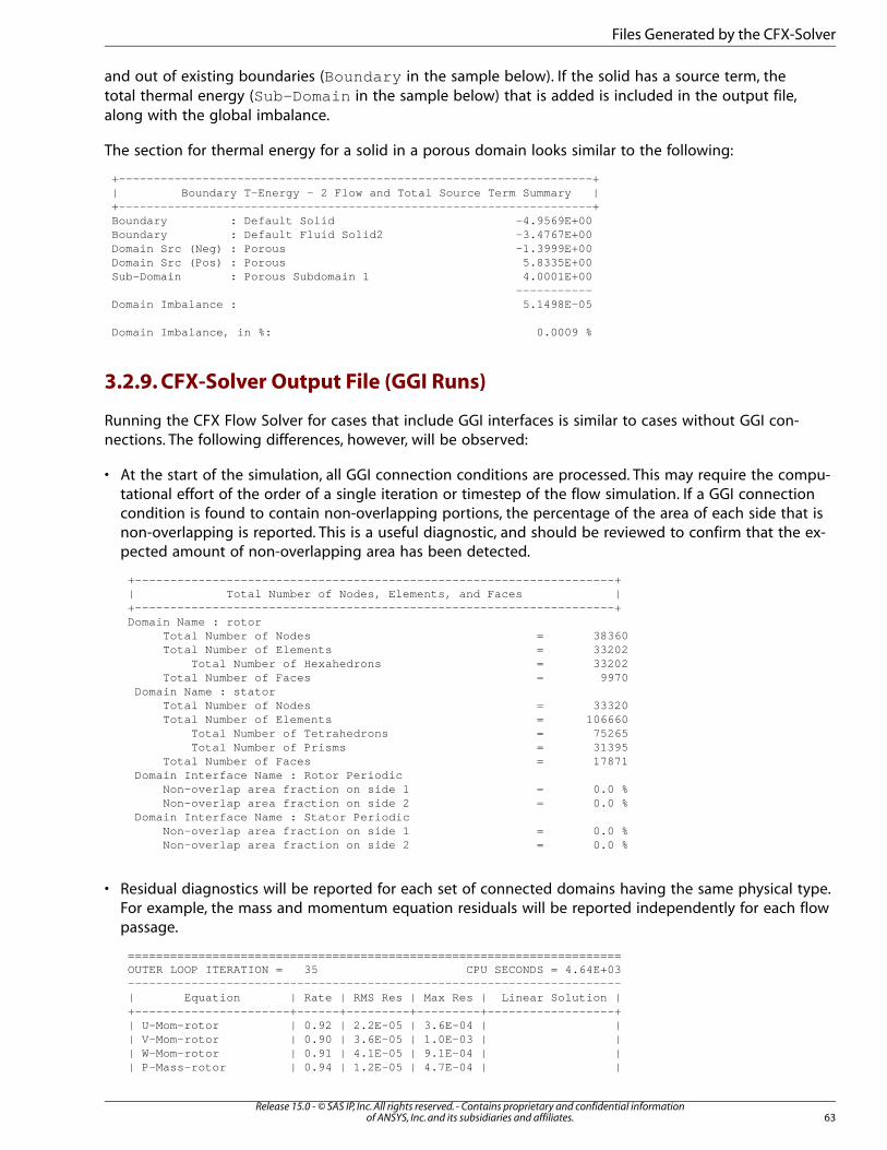
and out of existing boundaries (Boundary in the sample below). If the solid has a source term, thetotal thermal energy (Sub-Domain in the sample below) that is added is included in the output file,along with the global imbalance.
The section for thermal energy for a solid in a porous domain looks similar to the following:
+--------------------------------------------------------------------+| Boundary T-Energy - 2 Flow and Total Source Term Summary |+--------------------------------------------------------------------+Boundary : Default Solid -4.9569E+00Boundary : Default Fluid Solid2 -3.4767E+00Domain Src (Neg) : Porous -1.3999E+00Domain Src (Pos) : Porous 5.8335E+00Sub-Domain : Porous Subdomain 1 4.0001E+00 -----------Domain Imbalance : 5.1498E-05
Domain Imbalance, in %: 0.0009 %
3.2.9. CFX-Solver Output File (GGI Runs)
Running the CFX Flow Solver for cases that include GGI interfaces is similar to cases without GGI con-nections. The following differences, however, will be observed:
• At the start of the simulation, all GGI connection conditions are processed. This may require the compu-tational effort of the order of a single iteration or timestep of the flow simulation. If a GGI connectioncondition is found to contain non-overlapping portions, the percentage of the area of each side that isnon-overlapping is reported. This is a useful diagnostic, and should be reviewed to confirm that the ex-pected amount of non-overlapping area has been detected.
+--------------------------------------------------------------------+| Total Number of Nodes, Elements, and Faces |+--------------------------------------------------------------------+Domain Name : rotor Total Number of Nodes = 38360 Total Number of Elements = 33202 Total Number of Hexahedrons = 33202 Total Number of Faces = 9970 Domain Name : stator Total Number of Nodes = 33320 Total Number of Elements = 106660 Total Number of Tetrahedrons = 75265 Total Number of Prisms = 31395 Total Number of Faces = 17871 Domain Interface Name : Rotor Periodic Non-overlap area fraction on side 1 = 0.0 % Non-overlap area fraction on side 2 = 0.0 % Domain Interface Name : Stator Periodic Non-overlap area fraction on side 1 = 0.0 % Non-overlap area fraction on side 2 = 0.0 %
• Residual diagnostics will be reported for each set of connected domains having the same physical type.For example, the mass and momentum equation residuals will be reported independently for each flowpassage.
======================================================================OUTER LOOP ITERATION = 35 CPU SECONDS = 4.64E+03----------------------------------------------------------------------| Equation | Rate | RMS Res | Max Res | Linear Solution |+----------------------+------+---------+---------+------------------+| U-Mom-rotor | 0.92 | 2.2E-05 | 3.6E-04 | || V-Mom-rotor | 0.90 | 3.6E-05 | 1.0E-03 | || W-Mom-rotor | 0.91 | 4.1E-05 | 9.1E-04 | || P-Mass-rotor | 0.94 | 1.2E-05 | 4.7E-04 | |
63Release 15.0 - © SAS IP, Inc. All rights reserved. - Contains proprietary and confidential information
of ANSYS, Inc. and its subsidiaries and affiliates.
Files Generated by the CFX-Solver
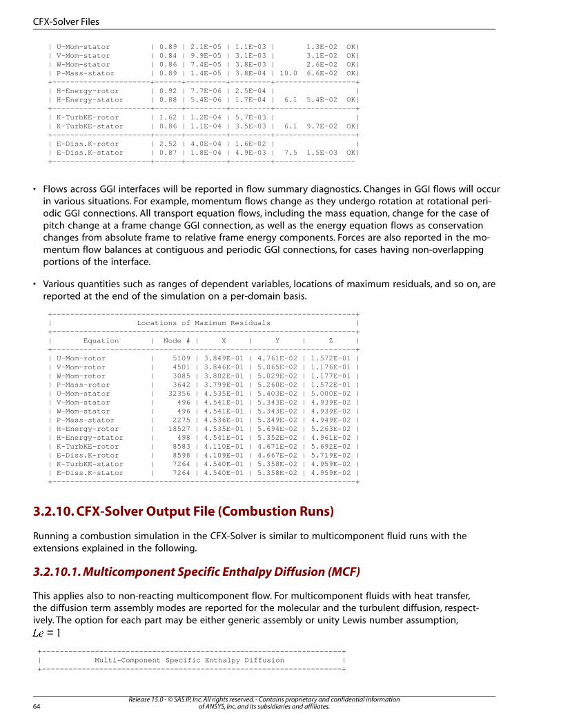
| U-Mom-stator | 0.89 | 2.1E-05 | 1.1E-03 | 1.3E-02 OK|| V-Mom-stator | 0.84 | 9.9E-05 | 3.1E-03 | 3.1E-02 OK|| W-Mom-stator | 0.86 | 7.4E-05 | 3.8E-03 | 2.6E-02 OK|| P-Mass-stator | 0.89 | 1.4E-05 | 3.8E-04 | 10.0 6.6E-02 OK|+----------------------+------+---------+---------+------------------+| H-Energy-rotor | 0.92 | 7.7E-06 | 2.5E-04 | || H-Energy-stator | 0.88 | 5.4E-06 | 1.7E-04 | 6.1 5.4E-02 OK|+----------------------+------+---------+---------+------------------+| K-TurbKE-rotor | 1.62 | 1.2E-04 | 5.7E-03 | || K-TurbKE-stator | 0.86 | 1.1E-04 | 3.5E-03 | 6.1 9.7E-02 OK|+----------------------+------+---------+---------+------------------+| E-Diss.K-rotor | 2.52 | 4.0E-04 | 1.6E-02 | || E-Diss.K-stator | 0.87 | 1.8E-04 | 4.9E-03 | 7.5 1.5E-03 OK|+----------------------+------+---------+---------+------------------
• Flows across GGI interfaces will be reported in flow summary diagnostics. Changes in GGI flows will occurin various situations. For example, momentum flows change as they undergo rotation at rotational peri-odic GGI connections. All transport equation flows, including the mass equation, change for the case ofpitch change at a frame change GGI connection, as well as the energy equation flows as conservationchanges from absolute frame to relative frame energy components. Forces are also reported in the mo-mentum flow balances at contiguous and periodic GGI connections, for cases having non-overlappingportions of the interface.
• Various quantities such as ranges of dependent variables, locations of maximum residuals, and so on, arereported at the end of the simulation on a per-domain basis.
+--------------------------------------------------------------------+| Locations of Maximum Residuals |+--------------------------------------------------------------------+| Equation | Node # | X | Y | Z |+--------------------------------------------------------------------+| U-Mom-rotor | 5109 | 3.849E-01 | 4.761E-02 | 1.572E-01 || V-Mom-rotor | 4501 | 3.846E-01 | 5.065E-02 | 1.176E-01 || W-Mom-rotor | 3085 | 3.802E-01 | 5.029E-02 | 1.177E-01 || P-Mass-rotor | 3642 | 3.799E-01 | 5.260E-02 | 1.572E-01 || U-Mom-stator | 32356 | 4.535E-01 | 5.403E-02 | 5.000E-02 || V-Mom-stator | 496 | 4.541E-01 | 5.343E-02 | 4.939E-02 || W-Mom-stator | 496 | 4.541E-01 | 5.343E-02 | 4.939E-02 || P-Mass-stator | 2275 | 4.536E-01 | 5.349E-02 | 4.949E-02 || H-Energy-rotor | 18527 | 4.535E-01 | 5.694E-02 | 5.263E-02 || H-Energy-stator | 498 | 4.541E-01 | 5.352E-02 | 4.961E-02 || K-TurbKE-rotor | 8583 | 4.110E-01 | 4.671E-02 | 5.692E-02 || E-Diss.K-rotor | 8598 | 4.109E-01 | 4.667E-02 | 5.719E-02 || K-TurbKE-stator | 7264 | 4.540E-01 | 5.358E-02 | 4.959E-02 || E-Diss.K-stator | 7264 | 4.540E-01 | 5.358E-02 | 4.959E-02 |+--------------------------------------------------------------------+
3.2.10. CFX-Solver Output File (Combustion Runs)
Running a combustion simulation in the CFX-Solver is similar to multicomponent fluid runs with theextensions explained in the following.
3.2.10.1. Multicomponent Specific Enthalpy Diffusion (MCF)
This applies also to non-reacting multicomponent flow. For multicomponent fluids with heat transfer,the diffusion term assembly modes are reported for the molecular and the turbulent diffusion, respect-ively. The option for each part may be either generic assembly or unity Lewis number assumption,
=��
+--------------------------------------------------------------------+| Multi-Component Specific Enthalpy Diffusion |+--------------------------------------------------------------------+
Release 15.0 - © SAS IP, Inc. All rights reserved. - Contains proprietary and confidential informationof ANSYS, Inc. and its subsidiaries and affiliates.64
CFX-Solver Files
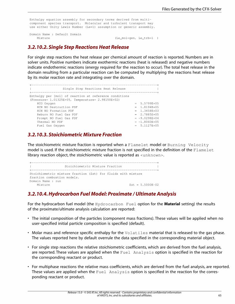
Enthalpy equation assembly for secondary terms derived from multi-component species transport. Molecular and turbulent transport mayuse either Unity Lewis Number (Le=1) assumption or generic assembly.
Domain Name : Default Domain Mixture (Le_mol=gen, Le_trb=1 )
3.2.10.2. Single Step Reactions Heat Release
For single step reactions the heat release per chemical amount of reaction is reported. Numbers are insolver units. Positive numbers indicate exothermic reactions (heat is released) and negative numbersindicate endothermic reactions (energy required for the reaction to occur). The total heat release in thedomain resulting from a particular reaction can be computed by multiplying the reactions heat releaseby its molar reaction rate and integrating over the domain.
+--------------------------------------------------------------------+| Single Step Reactions Heat Release |+--------------------------------------------------------------------+Enthalpy per [mol] of reaction at reference conditions(Pressure= 1.01325E+05, Temperature= 2.98150E+02) HCO Oxygen = 5.5799E+05 HCN NO Destruction PDF = 1.8194E+05 HCN NO Formation PDF = 1.3458E+03 Reburn NO Fuel Gas PDF = 2.7885E+05 Prompt NO Fuel Gas PDF = -9.0298E+04 Thermal NO PDF = -1.8060E+05 Fuel Gas Oxygen = 5.1127E+05
3.2.10.3. Stoichiometric Mixture Fraction
The stoichiometric mixture fraction is reported when a Flamelet model or Burning Velocitymodel is used. If the stoichiometric mixture fraction is not specified in the definition of the Flameletlibrary reaction object, the stoichiometric value is reported as <unknown> .
+--------------------------------------------------------------------+| Stoichiometric Mixture Fraction |+--------------------------------------------------------------------+Stoichiometric mixture fraction (Zst) for fluids with mixturefraction combustion models.Domain Name : run Mixture Zst = 5.5000E-02
3.2.10.4. Hydrocarbon Fuel Model: Proximate / Ultimate Analysis
For the hydrocarbon fuel model (the Hydrocarbon Fuel option for the Material setting) the resultsof the proximate/ultimate analysis calculation are reported:
• The initial composition of the particles (component mass fractions). These values will be applied when nouser-specified initial particle composition is specified (default).
• Molar mass and reference specific enthalpy for the Volatiles material that is released to the gas phase.The values reported here by default overrule the data specified in the corresponding material object.
• For single step reactions the relative stoichiometric coefficients, which are derived from the fuel analysis,are reported. These values are applied when the Fuel Analysis option is specified in the reaction forthe corresponding reactant or product.
• For multiphase reactions the relative mass coefficients, which are derived from the fuel analysis, are reported.These values are applied when the Fuel Analysis option is specified in the reaction for the corres-ponding reactant or product.
65Release 15.0 - © SAS IP, Inc. All rights reserved. - Contains proprietary and confidential information
of ANSYS, Inc. and its subsidiaries and affiliates.
Files Generated by the CFX-Solver
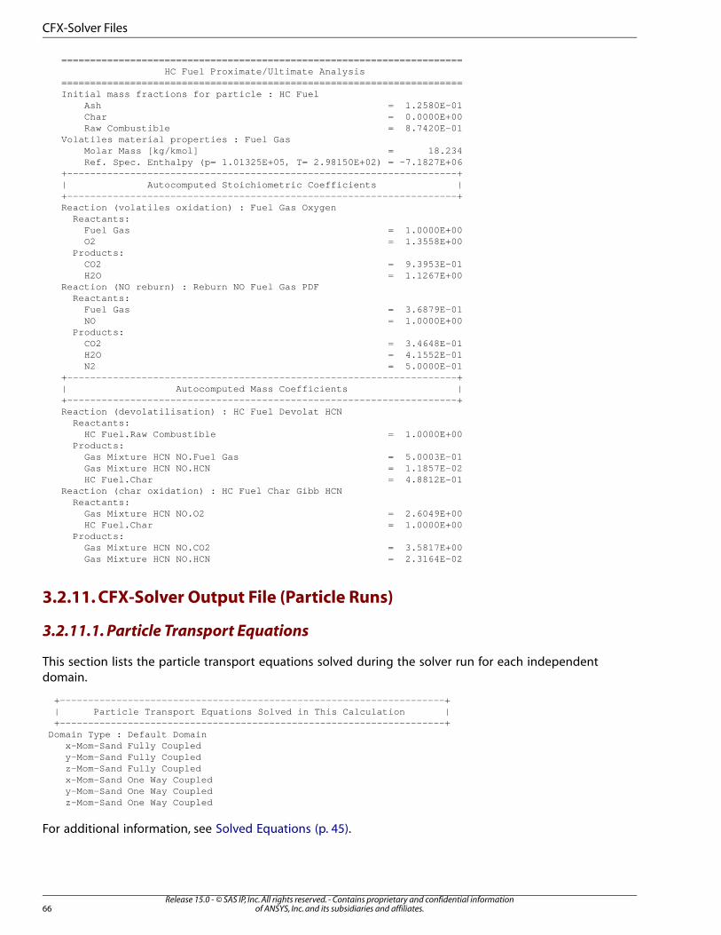
====================================================================== HC Fuel Proximate/Ultimate Analysis======================================================================Initial mass fractions for particle : HC Fuel Ash = 1.2580E-01 Char = 0.0000E+00 Raw Combustible = 8.7420E-01Volatiles material properties : Fuel Gas Molar Mass [kg/kmol] = 18.234 Ref. Spec. Enthalpy (p= 1.01325E+05, T= 2.98150E+02) = -7.1827E+06+--------------------------------------------------------------------+| Autocomputed Stoichiometric Coefficients |+--------------------------------------------------------------------+Reaction (volatiles oxidation) : Fuel Gas Oxygen Reactants: Fuel Gas = 1.0000E+00 O2 = 1.3558E+00 Products: CO2 = 9.3953E-01 H2O = 1.1267E+00Reaction (NO reburn) : Reburn NO Fuel Gas PDF Reactants: Fuel Gas = 3.6879E-01 NO = 1.0000E+00 Products: CO2 = 3.4648E-01 H2O = 4.1552E-01 N2 = 5.0000E-01+--------------------------------------------------------------------+| Autocomputed Mass Coefficients |+--------------------------------------------------------------------+Reaction (devolatilisation) : HC Fuel Devolat HCN Reactants: HC Fuel.Raw Combustible = 1.0000E+00 Products: Gas Mixture HCN NO.Fuel Gas = 5.0003E-01 Gas Mixture HCN NO.HCN = 1.1857E-02 HC Fuel.Char = 4.8812E-01Reaction (char oxidation) : HC Fuel Char Gibb HCN Reactants: Gas Mixture HCN NO.O2 = 2.6049E+00 HC Fuel.Char = 1.0000E+00 Products: Gas Mixture HCN NO.CO2 = 3.5817E+00 Gas Mixture HCN NO.HCN = 2.3164E-02
3.2.11. CFX-Solver Output File (Particle Runs)
3.2.11.1. Particle Transport Equations
This section lists the particle transport equations solved during the solver run for each independentdomain.
+--------------------------------------------------------------------+ | Particle Transport Equations Solved in This Calculation | +--------------------------------------------------------------------+Domain Type : Default Domain x-Mom-Sand Fully Coupled y-Mom-Sand Fully Coupled z-Mom-Sand Fully Coupled x-Mom-Sand One Way Coupled y-Mom-Sand One Way Coupled z-Mom-Sand One Way Coupled
For additional information, see Solved Equations (p. 45).
Release 15.0 - © SAS IP, Inc. All rights reserved. - Contains proprietary and confidential informationof ANSYS, Inc. and its subsidiaries and affiliates.66
CFX-Solver Files
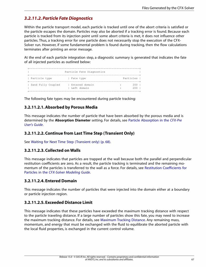
3.2.11.2. Particle Fate Diagnostics
Within the particle transport model, each particle is tracked until one of the abort criteria is satisfied orthe particle escapes the domain. Particles may also be aborted if a tracking error is found. Because eachparticle is tracked from its injection point until some abort criteria is met, it does not influence otherparticles. Thus, a tracking error for one particle does not necessarily stop the execution of the CFX-Solver run. However, if some fundamental problem is found during tracking, then the flow calculationsterminates after printing an error message.
At the end of each particle integration step, a diagnostic summary is generated that indicates the fateof all injected particles as outlined below:
+--------------------------------------------------------------------+ | Particle Fate Diagnostics | +--------------------------------------------------------------------+ | Particle type | Fate type Particles | +--------------------------------------------------------------------+ | Sand Fully Coupled | Entered domain : 200 | | | Left domain : 200 | +--------------------------------------------------------------------+
The following fate types may be encountered during particle tracking:
3.2.11.2.1. Absorbed by Porous Media
This message indicates the number of particle that have been absorbed by the porous media and isdetermined by the Absorption Diameter setting. For details, see Particle Absorption in the CFX-Pre
User's Guide.
3.2.11.2.2. Continue from Last Time Step (Transient Only)
See Waiting for Next Time Step (Transient only) (p. 68).
3.2.11.2.3. Collected on Walls
This message indicates that particles are trapped at the wall because both the parallel and perpendicularrestitution coefficients are zero. As a result, the particle tracking is terminated and the remaining mo-mentum of the particles is transferred to the wall as a force. For details, see Restitution Coefficients forParticles in the CFX-Solver Modeling Guide.
3.2.11.2.4. Entered Domain
This message indicates the number of particles that were injected into the domain either at a boundaryor particle injection region.
3.2.11.2.5. Exceeded Distance Limit
This message indicates that these particles have exceeded the maximum tracking distance with respectto the particle traveling distance. If a large number of particles show this fate, you may need to increasethe maximum tracking distance. For details, see Maximum Tracking Distance. Any remaining mass,momentum, and energy that must be exchanged with the fluid to equilibrate the aborted particle withthe local fluid properties, is exchanged in the current control volume.
67Release 15.0 - © SAS IP, Inc. All rights reserved. - Contains proprietary and confidential information
of ANSYS, Inc. and its subsidiaries and affiliates.
Files Generated by the CFX-Solver
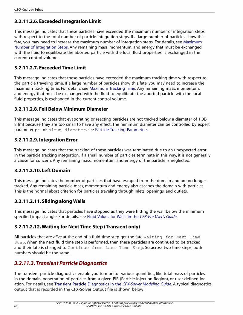
3.2.11.2.6. Exceeded Integration Limit
This message indicates that these particles have exceeded the maximum number of integration stepswith respect to the total number of particle integration steps. If a large number of particles show thisfate, you may need to increase the maximum number of integration steps. For details, see MaximumNumber of Integration Steps. Any remaining mass, momentum, and energy that must be exchangedwith the fluid to equilibrate the aborted particle with the local fluid properties, is exchanged in thecurrent control volume.
3.2.11.2.7. Exceeded Time Limit
This message indicates that these particles have exceeded the maximum tracking time with respect tothe particle traveling time. If a large number of particles show this fate, you may need to increase themaximum tracking time. For details, see Maximum Tracking Time. Any remaining mass, momentum,and energy that must be exchanged with the fluid to equilibrate the aborted particle with the localfluid properties, is exchanged in the current control volume.
3.2.11.2.8. Fell Below Minimum Diameter
This message indicates that evaporating or reacting particles are not tracked below a diameter of 1.0E-8 [m] because they are too small to have any effect. The minimum diameter can be controlled by expertparameter pt minimum diameter , see Particle Tracking Parameters.
3.2.11.2.9. Integration Error
This message indicates that the tracking of these particles was terminated due to an unexpected errorin the particle tracking integration. If a small number of particles terminate in this way, it is not generallya cause for concern. Any remaining mass, momentum, and energy of the particle is neglected.
3.2.11.2.10. Left Domain
This message indicates the number of particles that have escaped from the domain and are no longertracked. Any remaining particle mass, momentum and energy also escapes the domain with particles.This is the normal abort criterion for particles traveling through inlets, openings, and outlets.
3.2.11.2.11. Sliding along Walls
This message indicates that particles have stopped as they were hitting the wall below the minimumspecified impact angle. For details, see Fluid Values for Walls in the CFX-Pre User's Guide.
3.2.11.2.12. Waiting for Next Time Step (Transient only)
All particles that are alive at the end of a fluid time step get the fate Waiting for Next TimeStep . When the next fluid time step is performed, then these particles are continued to be trackedand their fate is changed to Continue from Last Time Step . So across two time steps, bothnumbers should be the same.
3.2.11.3. Transient Particle Diagnostics
The transient particle diagnostics enable you to monitor various quantities, like total mass of particlesin the domain, penetration of particles from a given PIR (Particle Injection Region), or user-defined loc-ation. For details, see Transient Particle Diagnostics in the CFX-Solver Modeling Guide. A typical diagnosticsoutput that is recorded in the CFX-Solver Output file is shown below:
Release 15.0 - © SAS IP, Inc. All rights reserved. - Contains proprietary and confidential informationof ANSYS, Inc. and its subsidiaries and affiliates.68
CFX-Solver Files
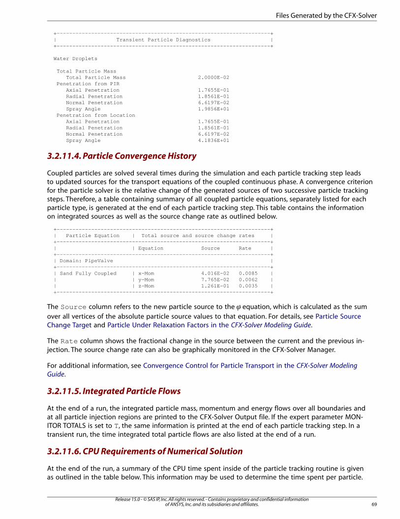
+--------------------------------------------------------------------+ | Transient Particle Diagnostics | +--------------------------------------------------------------------+
Water Droplets
Total Particle Mass Total Particle Mass 2.0000E-02 Penetration from PIR Axial Penetration 1.7655E-01 Radial Penetration 1.8561E-01 Normal Penetration 6.6197E-02 Spray Angle 1.9856E+01 Penetration from Location Axial Penetration 1.7655E-01 Radial Penetration 1.8561E-01 Normal Penetration 6.6197E-02 Spray Angle 4.1836E+01
3.2.11.4. Particle Convergence History
Coupled particles are solved several times during the simulation and each particle tracking step leadsto updated sources for the transport equations of the coupled continuous phase. A convergence criterionfor the particle solver is the relative change of the generated sources of two successive particle trackingsteps. Therefore, a table containing summary of all coupled particle equations, separately listed for eachparticle type, is generated at the end of each particle tracking step. This table contains the informationon integrated sources as well as the source change rate as outlined below.
+--------------------------------------------------------------------+ | Particle Equation | Total source and source change rates | +--------------------------------------------------------------------+ | | Equation Source Rate | +--------------------------------------------------------------------+ | Domain: PipeValve | +--------------------------------------------------------------------+ | Sand Fully Coupled | x-Mom 4.016E-02 0.0085 | | | y-Mom 7.765E-02 0.0062 | | | z-Mom 1.261E-01 0.0035 | +--------------------------------------------------------------------+
The Source column refers to the new particle source to the � equation, which is calculated as the sum
over all vertices of the absolute particle source values to that equation. For details, see Particle SourceChange Target and Particle Under Relaxation Factors in the CFX-Solver Modeling Guide.
The Rate column shows the fractional change in the source between the current and the previous in-jection. The source change rate can also be graphically monitored in the CFX-Solver Manager.
For additional information, see Convergence Control for Particle Transport in the CFX-Solver Modeling
Guide.
3.2.11.5. Integrated Particle Flows
At the end of a run, the integrated particle mass, momentum and energy flows over all boundaries andat all particle injection regions are printed to the CFX-Solver Output file. If the expert parameter MON-ITOR TOTALS is set to T, the same information is printed at the end of each particle tracking step. In atransient run, the time integrated total particle flows are also listed at the end of a run.
3.2.11.6. CPU Requirements of Numerical Solution
At the end of the run, a summary of the CPU time spent inside of the particle tracking routine is givenas outlined in the table below. This information may be used to determine the time spent per particle.
69Release 15.0 - © SAS IP, Inc. All rights reserved. - Contains proprietary and confidential information
of ANSYS, Inc. and its subsidiaries and affiliates.
Files Generated by the CFX-Solver

+--------------------------------------------------------------------+| CPU Requirements of Numerical Solution |+--------------------------------------------------------------------+
Subsystem Name Discretization Linear Solution (secs. %total) (secs. %total) ---------------------------------------------------------------------- Momentum and Mass 1.00E+02 48.2 % 1.79E+01 8.6 % TurbKE and Diss.K 3.46E+01 16.6 % 2.17E+01 10.4 % -------- ------- -------- ------ Subsystem Summary 1.35E+02 64.9 % 3.96E+01 19.1 %
Particle Tracking 2.18E+01 10.5 % Variable Updates 5.91E+00 2.8 % File Reading 6.25E-02 0.0 % Miscellaneous 5.72E+00 2.7 % -------- Total 2.08E+02
3.2.12. CFX-Solver Output File (ANSYS Multi-field Runs)
An ANSYS Multi-field run can be launched from the CFX-Solver Manager (or from the command lineusing the cfx5solve command) or from the ANSYS CFX Launcher. Some content is added to theoutput file for all ANSYS Multi-field runs, and extra content is added in the case of a run launched byCFX.
If the ANSYS input file is processed, then this is noted in the output file, and the location of the newinput file that is created is recorded.
+--------------------------------------------------------------------+| || Processing ANSYS Input File (Running CCL2MF) || |+--------------------------------------------------------------------+Created /home3/cfdsjw/tmp/comp/StaticMixer_001.ansys/ANSYS.mf
If the ANSYS Solver was started by CFX, then this is also noted in the output file.
+--------------------------------------------------------------------+| || Starting ANSYS Solver || |+--------------------------------------------------------------------+
The host name and port number used by CFX-Solver to communicate to the ANSYS Solver is recorded.If you started only CFX-Solver using the CFX-Solver Manager or the command line, then you will haveprovided these; otherwise, the port number is determined automatically by the ANSYS Solver andcommunicated to CFX-Solver by the start-up script.
Connecting to the following master process: Host Name : sceptre Port Number : 34586
Information on what data will be exchanged on what boundaries is recorded so that you can checkthat all is as you expect it to be.
+--------------------------------------------------------------------+| Boundary Condition Data Supplied by External Solver Coupling |+--------------------------------------------------------------------+ANSYS Multi-field Solver : ANSYS CFX Boundary : Interface CFX Variable : Total Mesh Displacement ANSYS Interface : 1 ANSYS Variable : DISP
For steady-state runs only, each time a new coupling step begins, it is noted in the output file.
Release 15.0 - © SAS IP, Inc. All rights reserved. - Contains proprietary and confidential informationof ANSYS, Inc. and its subsidiaries and affiliates.70
CFX-Solver Files
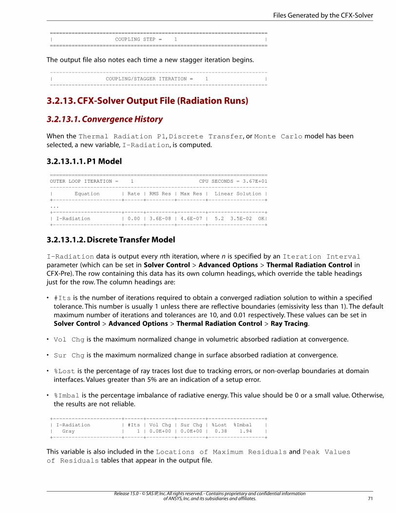
======================================================================| COUPLING STEP = 1 |======================================================================
The output file also notes each time a new stagger iteration begins.
----------------------------------------------------------------------| COUPLING/STAGGER ITERATION = 1 |----------------------------------------------------------------------
3.2.13. CFX-Solver Output File (Radiation Runs)
3.2.13.1. Convergence History
When the Thermal Radiation P1 , Discrete Transfer , or Monte Carlo model has beenselected, a new variable, I-Radiation , is computed.
3.2.13.1.1. P1 Model
======================================================================OUTER LOOP ITERATION = 1 CPU SECONDS = 3.67E+01----------------------------------------------------------------------| Equation | Rate | RMS Res | Max Res | Linear Solution |+----------------------+------+---------+---------+------------------+...+----------------------+------+---------+---------+------------------+| I-Radiation | 0.00 | 3.6E-08 | 4.6E-07 | 5.2 3.5E-02 OK|+----------------------+------+---------+---------+------------------+
3.2.13.1.2. Discrete Transfer Model
I-Radiation data is output every nth iteration, where n is specified by an Iteration Intervalparameter (which can be set in Solver Control > Advanced Options > Thermal Radiation Control inCFX-Pre). The row containing this data has its own column headings, which override the table headingsjust for the row. The column headings are:
• #Its is the number of iterations required to obtain a converged radiation solution to within a specifiedtolerance. This number is usually 1 unless there are reflective boundaries (emissivity less than 1). The defaultmaximum number of iterations and tolerances are 10, and 0.01 respectively. These values can be set inSolver Control > Advanced Options > Thermal Radiation Control > Ray Tracing.
• Vol Chg is the maximum normalized change in volumetric absorbed radiation at convergence.
• Sur Chg is the maximum normalized change in surface absorbed radiation at convergence.
• %Lost is the percentage of ray traces lost due to tracking errors, or non-overlap boundaries at domaininterfaces. Values greater than 5% are an indication of a setup error.
• %Imbal is the percentage imbalance of radiative energy. This value should be 0 or a small value. Otherwise,the results are not reliable.
+----------------------+------+---------+---------+------------------+| I-Radiation | #Its | Vol Chg | Sur Chg | %Lost %Imbal || Gray | 1 | 0.0E+00 | 0.0E+00 | 0.38 1.94 |+----------------------+------+---------+---------+------------------+
This variable is also included in the Locations of Maximum Residuals and Peak Valuesof Residuals tables that appear in the output file.
71Release 15.0 - © SAS IP, Inc. All rights reserved. - Contains proprietary and confidential information
of ANSYS, Inc. and its subsidiaries and affiliates.
Files Generated by the CFX-Solver
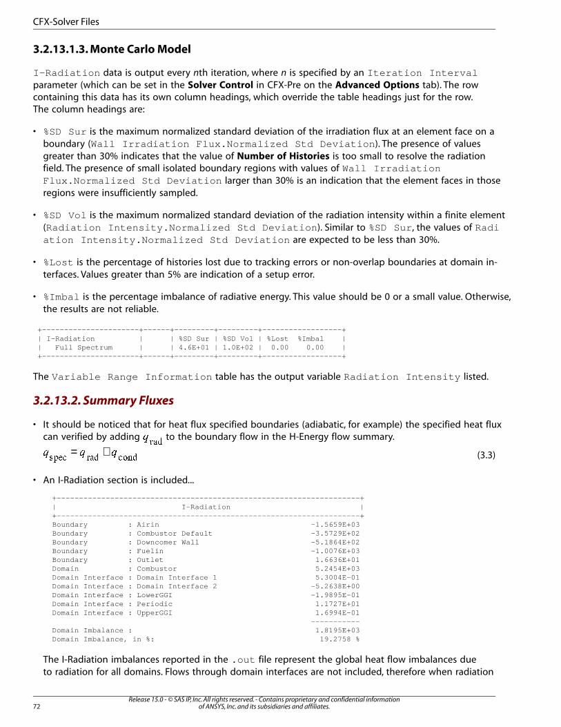
3.2.13.1.3. Monte Carlo Model
I-Radiation data is output every nth iteration, where n is specified by an Iteration Intervalparameter (which can be set in the Solver Control in CFX-Pre on the Advanced Options tab). The rowcontaining this data has its own column headings, which override the table headings just for the row.The column headings are:
• %SD Sur is the maximum normalized standard deviation of the irradiation flux at an element face on aboundary (Wall Irradiation Flux.Normalized Std Deviation ). The presence of valuesgreater than 30% indicates that the value of Number of Histories is too small to resolve the radiationfield. The presence of small isolated boundary regions with values of Wall IrradiationFlux.Normalized Std Deviation larger than 30% is an indication that the element faces in thoseregions were insufficiently sampled.
• %SD Vol is the maximum normalized standard deviation of the radiation intensity within a finite element(Radiation Intensity.Normalized Std Deviation ). Similar to %SD Sur , the values of Radiation Intensity.Normalized Std Deviation are expected to be less than 30%.
• %Lost is the percentage of histories lost due to tracking errors or non-overlap boundaries at domain in-terfaces. Values greater than 5% are indication of a setup error.
• %Imbal is the percentage imbalance of radiative energy. This value should be 0 or a small value. Otherwise,the results are not reliable.
+----------------------+------+---------+---------+------------------+| I-Radiation | | %SD Sur | %SD Vol | %Lost %Imbal || Full Spectrum | | 4.6E+01 | 1.0E+02 | 0.00 0.00 |+----------------------+------+---------+---------+------------------+
The Variable Range Information table has the output variable Radiation Intensity listed.
3.2.13.2. Summary Fluxes
• It should be noticed that for heat flux specified boundaries (adiabatic, for example) the specified heat fluxcan verified by adding �
��� to the boundary flow in the H-Energy flow summary.
(3.3)= +� � ����� � �� �
• An I-Radiation section is included...
+--------------------------------------------------------------------+ | I-Radiation | +--------------------------------------------------------------------+ Boundary : Airin -1.5659E+03 Boundary : Combustor Default -3.5729E+02 Boundary : Downcomer Wall -5.1864E+02 Boundary : Fuelin -1.0076E+03 Boundary : Outlet 1.6636E+01 Domain : Combustor 5.2454E+03 Domain Interface : Domain Interface 1 5.3004E-01 Domain Interface : Domain Interface 2 -5.2638E+00 Domain Interface : LowerGGI -1.9895E-01 Domain Interface : Periodic 1.1727E+01 Domain Interface : UpperGGI 1.6994E-01 ----------- Domain Imbalance : 1.8195E+03 Domain Imbalance, in %: 19.2758 %
The I-Radiation imbalances reported in the .out file represent the global heat flow imbalances dueto radiation for all domains. Flows through domain interfaces are not included, therefore when radiation
Release 15.0 - © SAS IP, Inc. All rights reserved. - Contains proprietary and confidential informationof ANSYS, Inc. and its subsidiaries and affiliates.72
CFX-Solver Files
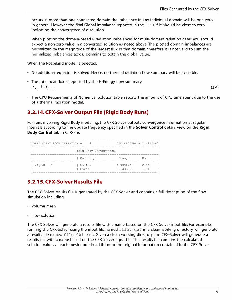
occurs in more than one connected domain the imbalance in any individual domain will be non-zeroin general. However, the final Global Imbalance reported in the .out file should be close to zero,indicating the convergence of a solution.
When plotting the domain-based I-Radiation imbalances for multi-domain radiation cases you shouldexpect a non-zero value in a converged solution as noted above. The plotted domain imbalances arenormalized by the magnitude of the largest flux in that domain, therefore it is not valid to sum thenormalized imbalances across domains to obtain the global value.
When the Rosseland model is selected:
• No additional equation is solved. Hence, no thermal radiation flow summary will be available.
• The total heat flux is reported by the H-Energy flow summary.
(3.4)+� ���� ����
• The CPU Requirements of Numerical Solution table reports the amount of CPU time spent due to the useof a thermal radiation model.
3.2.14. CFX-Solver Output File (Rigid Body Runs)
For runs involving Rigid Body modeling, the CFX-Solver outputs convergence information at regularintervals according to the update frequency specified in the Solver Control details view on the Rigid
Body Control tab in CFX-Pre.
---------------------------------------------------------------------- COEFFICIENT LOOP ITERATION = 5 CPU SECONDS = 1.461E+01 ---------------------------------------------------------------------- | Rigid Body Convergence | +--------------------------------------------------------------------+ | | Quantity Change Rate | +--------------------------------------------------------------------+ | rigidBody1 | Motion 1.783E-01 0.26 | | | Force 7.343E-01 1.04 | +--------------------------------------------------------------------+
3.2.15. CFX-Solver Results File
The CFX-Solver results file is generated by the CFX-Solver and contains a full description of the flowsimulation including:
• Volume mesh
• Flow solution
The CFX-Solver will generate a results file with a name based on the CFX-Solver input file. For example,running the CFX-Solver using the input file named file.mdef in a clean working directory will generatea results file named file_001.res . Given a clean working directory, the CFX-Solver will generate aresults file with a name based on the CFX-Solver input file. This results file contains the calculatedsolution values at each mesh node in addition to the original information contained in the CFX-Solver
73Release 15.0 - © SAS IP, Inc. All rights reserved. - Contains proprietary and confidential information
of ANSYS, Inc. and its subsidiaries and affiliates.
Files Generated by the CFX-Solver
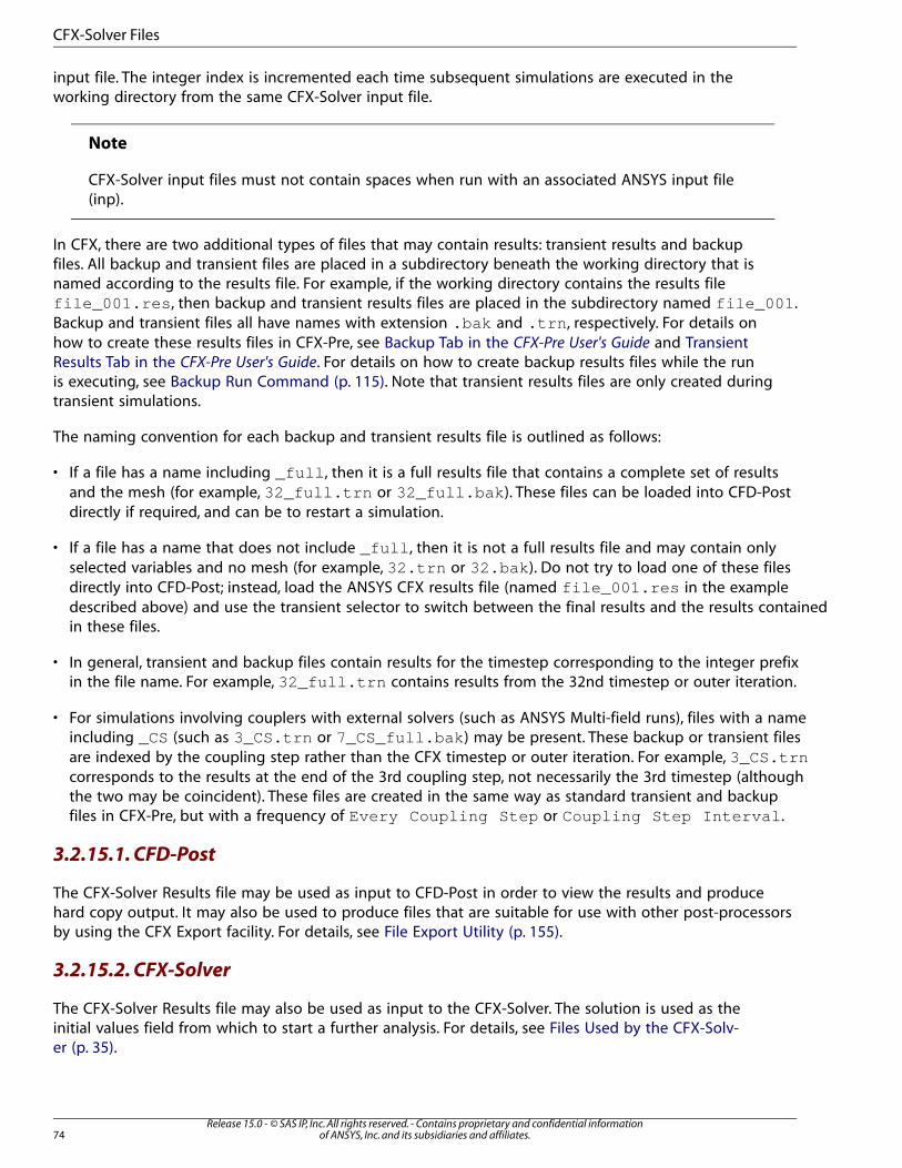
input file. The integer index is incremented each time subsequent simulations are executed in theworking directory from the same CFX-Solver input file.
Note
CFX-Solver input files must not contain spaces when run with an associated ANSYS input file(inp).
In CFX, there are two additional types of files that may contain results: transient results and backupfiles. All backup and transient files are placed in a subdirectory beneath the working directory that isnamed according to the results file. For example, if the working directory contains the results filefile_001.res , then backup and transient results files are placed in the subdirectory named file_001 .Backup and transient files all have names with extension .bak and .trn , respectively. For details onhow to create these results files in CFX-Pre, see Backup Tab in the CFX-Pre User's Guide and TransientResults Tab in the CFX-Pre User's Guide. For details on how to create backup results files while the runis executing, see Backup Run Command (p. 115). Note that transient results files are only created duringtransient simulations.
The naming convention for each backup and transient results file is outlined as follows:
• If a file has a name including _full , then it is a full results file that contains a complete set of resultsand the mesh (for example, 32_full.trn or 32_full.bak ). These files can be loaded into CFD-Postdirectly if required, and can be to restart a simulation.
• If a file has a name that does not include _full , then it is not a full results file and may contain onlyselected variables and no mesh (for example, 32.trn or 32.bak ). Do not try to load one of these filesdirectly into CFD-Post; instead, load the ANSYS CFX results file (named file_001.res in the exampledescribed above) and use the transient selector to switch between the final results and the results containedin these files.
• In general, transient and backup files contain results for the timestep corresponding to the integer prefixin the file name. For example, 32_full.trn contains results from the 32nd timestep or outer iteration.
• For simulations involving couplers with external solvers (such as ANSYS Multi-field runs), files with a nameincluding _CS (such as 3_CS.trn or 7_CS_full.bak ) may be present. These backup or transient filesare indexed by the coupling step rather than the CFX timestep or outer iteration. For example, 3_CS.trncorresponds to the results at the end of the 3rd coupling step, not necessarily the 3rd timestep (althoughthe two may be coincident). These files are created in the same way as standard transient and backupfiles in CFX-Pre, but with a frequency of Every Coupling Step or Coupling Step Interval .
3.2.15.1. CFD-Post
The CFX-Solver Results file may be used as input to CFD-Post in order to view the results and producehard copy output. It may also be used to produce files that are suitable for use with other post-processorsby using the CFX Export facility. For details, see File Export Utility (p. 155).
3.2.15.2. CFX-Solver
The CFX-Solver Results file may also be used as input to the CFX-Solver. The solution is used as theinitial values field from which to start a further analysis. For details, see Files Used by the CFX-Solv-er (p. 35).
Release 15.0 - © SAS IP, Inc. All rights reserved. - Contains proprietary and confidential informationof ANSYS, Inc. and its subsidiaries and affiliates.74
CFX-Solver Files
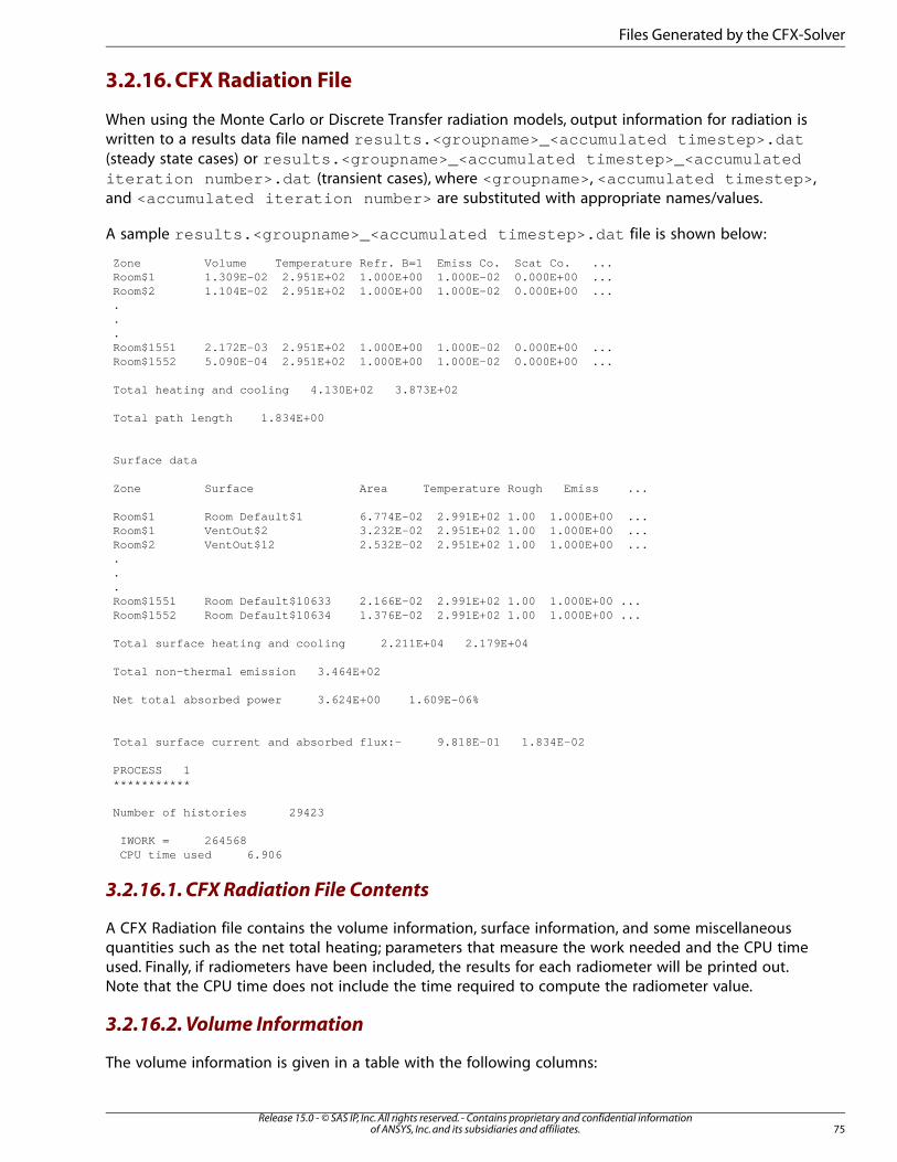
3.2.16. CFX Radiation File
When using the Monte Carlo or Discrete Transfer radiation models, output information for radiation iswritten to a results data file named results.<groupname>_<accumulated timestep>.dat(steady state cases) or results.<groupname>_<accumulated timestep>_<accumulatediteration number>.dat (transient cases), where <groupname> , <accumulated timestep> ,and <accumulated iteration number> are substituted with appropriate names/values.
A sample results.<groupname>_<accumulated timestep>.dat file is shown below:
Zone Volume Temperature Refr. B=1 Emiss Co. Scat Co. ...Room$1 1.309E-02 2.951E+02 1.000E+00 1.000E-02 0.000E+00 ...Room$2 1.104E-02 2.951E+02 1.000E+00 1.000E-02 0.000E+00 ......Room$1551 2.172E-03 2.951E+02 1.000E+00 1.000E-02 0.000E+00 ...Room$1552 5.090E-04 2.951E+02 1.000E+00 1.000E-02 0.000E+00 ...
Total heating and cooling 4.130E+02 3.873E+02
Total path length 1.834E+00
Surface data
Zone Surface Area Temperature Rough Emiss ...
Room$1 Room Default$1 6.774E-02 2.991E+02 1.00 1.000E+00 ...Room$1 VentOut$2 3.232E-02 2.951E+02 1.00 1.000E+00 ...Room$2 VentOut$12 2.532E-02 2.951E+02 1.00 1.000E+00 ......Room$1551 Room Default$10633 2.166E-02 2.991E+02 1.00 1.000E+00 ...Room$1552 Room Default$10634 1.376E-02 2.991E+02 1.00 1.000E+00 ...
Total surface heating and cooling 2.211E+04 2.179E+04
Total non-thermal emission 3.464E+02
Net total absorbed power 3.624E+00 1.609E-06%
Total surface current and absorbed flux:- 9.818E-01 1.834E-02
PROCESS 1***********
Number of histories 29423
IWORK = 264568 CPU time used 6.906
3.2.16.1. CFX Radiation File Contents
A CFX Radiation file contains the volume information, surface information, and some miscellaneousquantities such as the net total heating; parameters that measure the work needed and the CPU timeused. Finally, if radiometers have been included, the results for each radiometer will be printed out.Note that the CPU time does not include the time required to compute the radiometer value.
3.2.16.2. Volume Information
The volume information is given in a table with the following columns:
75Release 15.0 - © SAS IP, Inc. All rights reserved. - Contains proprietary and confidential information
of ANSYS, Inc. and its subsidiaries and affiliates.
Files Generated by the CFX-Solver
• Zone is the radiation element’s internal name
• Volume is the volume of the radiation element
• Temperature is the temperature of the element
• Refr. B=1 is the refractive index of the element
• Emiss Co. is the emission coefficient (Units: per length)
• Scat Co. is the scattering opacity coefficient (Units: per length)
• Path len. is the average length when crossing a radiation element
• Heating is average volumetric absorbed radiation
• Emission is the volumetric emitted radiation
• (H-E)*VOL is the amount of radiative energy that shows up as a square term in the energy equation
• Error % is the standard deviation of the path length.
For non-gray models the emission and scattering coefficients are the spectrum integrated coefficients.In a gray model the absorption coefficient equals the emission coefficient, in a non-gray model it canbe obtained from the intensity and the heating.
The next five columns contain the results. The seventh is the total path length of photons in the zone(Monte Carlo) or the mean radiation intensity (discrete transfer). The eighth is the heating per unitvolume, the ninth the cooling per unit volume, and the tenth the net total radiative heating rate forthe zone. The last column gives the statistical percentage error for Monte Carlo or the number of samples(rays traced through the zone) used for the heating quadrature in the discrete transfer case.
Finally comes the total heating and cooling rates for the entire volume and, for Monte Carlo, the totalmean path length of photons in the geometry. Non-gray models will also have the band by bandcooling.
3.2.16.3. Surface Information
In this output the first column is the zone name and the second the surface name. The third is thesurface temperature, the fourth the surface roughness and the fifth is the surface emissivity, spectrumintegrated in the case of a non-gray model. Grey surfaces have an albedo equal to one minus theemissivity, in the non-gray case the integrated albedo can be obtained from the surface heating andthe incident flux.
The next five columns contain the results. The sixth is the surface current (Monte Carlo) or average in-cident radiation flux (discrete transfer). The seventh is the heating per unit area, the eighth the coolingper unit area and the ninth the net total radiative heating. The last column is the statistical error (MonteCarlo) or the number of surface nodes used for sampling (discrete transfer).
Finally comes the total heating and cooling rates for all the surfaces in the geometry. Non-gray modelswill also show the band by band cooling.
After the above information, the overall net heating for the model is printed. This is a measure of howgood the calculation was because this figure should be zero. For a Monte Carlo calculation the totalsurface current and absorbed photon flux is printed, these figures should sum to unity and can therefore
Release 15.0 - © SAS IP, Inc. All rights reserved. - Contains proprietary and confidential informationof ANSYS, Inc. and its subsidiaries and affiliates.76
CFX-Solver Files
be used as another measure of the accuracy of the calculation. Next the number of histories computed(Monte Carlo) or the number of angular ordinates (Discrete transfer) is printed. The last numbers arethe work estimator and the CPU time. The work estimator is defined in terms of units of work where aunit of work is the computational effort to trace a photon (ray) to the next event (surface) and processthat event (update the recursion relation) for Monte Carlo (Discrete transfer). If radiometers have beencalculated, the angular calibration table that is used will be printed; then for each radiometer location,the following will be written: location, direction, temperature, flux.
3.2.17. CFX Partition File
The CFX partition file is generated by the CFX-Solver and used as input for a parallel run. The partitionfile is used to store information about the partitioning of the mesh. The partition file can be used toview mesh partitions before running the CFX-Solver. To do this, set the expert parameter writepartition number=t before partitioning, then combine the partition file with the CFX-Solver inputfile that was used to produce the partition file.
On UNIX systems, type:
cat filename.def filename_001.par > newfilename.res
On Windows systems, type:
copy /b filename.def + filename_001.par newfilename.res
This creates a results file that can be loaded in CFD-Post and contains the variable Real partitionnumber .
Note
A partition file generated in ANSYS CFX 11.0 or earlier versions is not supported in ANSYSCFX 12.0. If such a file is used in ANSYS CFX 12.0, then an error message is generated.
3.2.18. Additional Files for ANSYS Multi-field Runs
For an ANSYS Multi-field run, the CFX-Solver does not produce any extra files. However, if the ANSYSSolver is launched by CFX, a new directory with a name of the form <Run Name>.ansys is created.This is used as the ANSYS working directory and many files will be created here by ANSYS. In addition,the CFX processing of the ANSYS files produces two extra files:
• Components File - this has a name of the form *.cm and can be found in the ANSYS working directory.It is created to contain some region definitions for CFD-Post when it reads the ANSYS results files. Fordetails, see ANSYS Files in the CFD-Post User's Guide.
• ANSYS Multi-field input file - this has a name of the form *.mf and can be found in the ANSYS workingdirectory. It is created whenever you ask for the provided ANSYS input file to be processed as part of de-fining a run. It contains the ANSYS setup (solid physics) together with the multi-field commands that areconstructed from the ANSYS Multi-field settings in the CFX-Solver input file. For details, see Processingthe ANSYS Input File (p. 29).
3.2.19. CFX Multi-Configuration Output File
Multi-configuration simulations involve the sequential and sometimes repeated execution of definedconfigurations. The CFX-Solver generates a multi-configuration output file to summarize the globalproblem definition and execution of configurations.
77Release 15.0 - © SAS IP, Inc. All rights reserved. - Contains proprietary and confidential information
of ANSYS, Inc. and its subsidiaries and affiliates.
Files Generated by the CFX-Solver
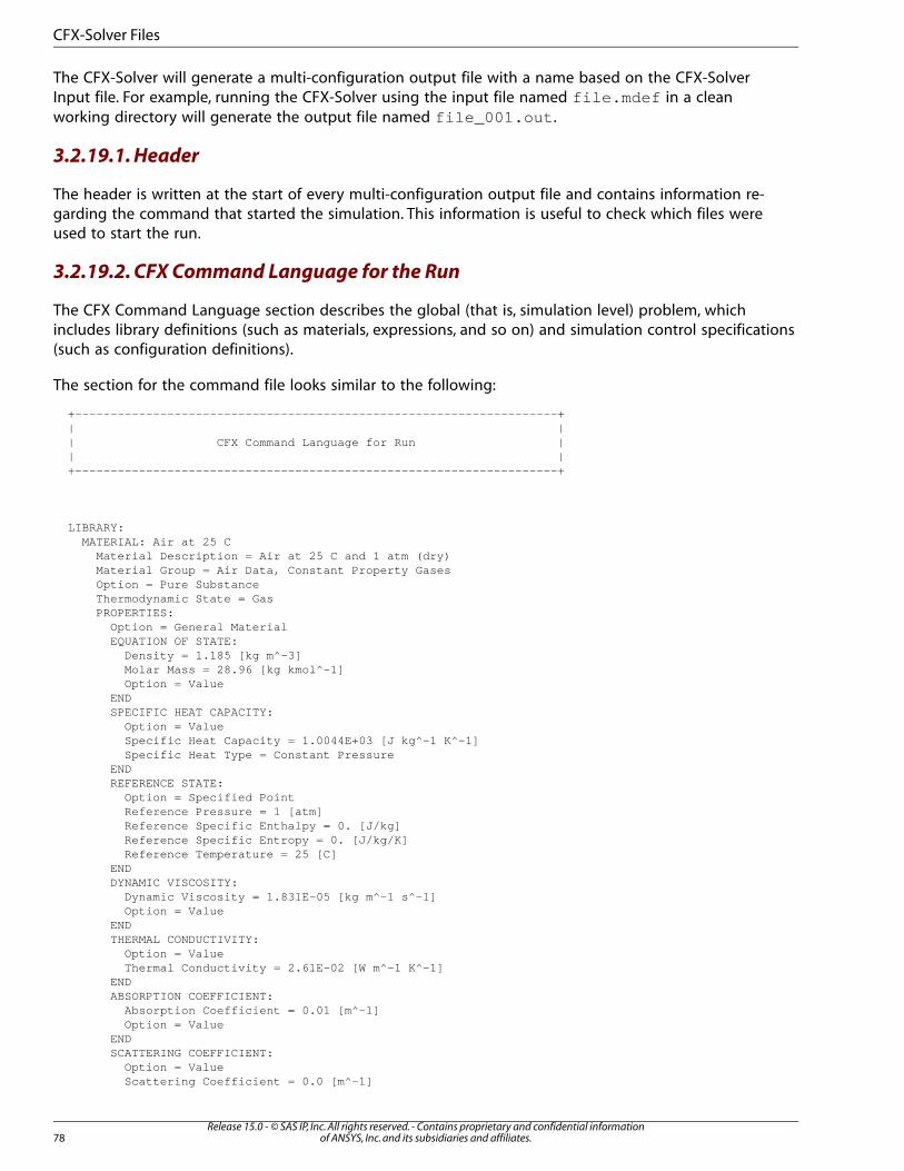
The CFX-Solver will generate a multi-configuration output file with a name based on the CFX-SolverInput file. For example, running the CFX-Solver using the input file named file.mdef in a cleanworking directory will generate the output file named file_001.out .
3.2.19.1. Header
The header is written at the start of every multi-configuration output file and contains information re-garding the command that started the simulation. This information is useful to check which files wereused to start the run.
3.2.19.2. CFX Command Language for the Run
The CFX Command Language section describes the global (that is, simulation level) problem, whichincludes library definitions (such as materials, expressions, and so on) and simulation control specifications(such as configuration definitions).
The section for the command file looks similar to the following:
+--------------------------------------------------------------------+ | | | CFX Command Language for Run | | | +--------------------------------------------------------------------+
LIBRARY: MATERIAL: Air at 25 C Material Description = Air at 25 C and 1 atm (dry) Material Group = Air Data, Constant Property Gases Option = Pure Substance Thermodynamic State = Gas PROPERTIES: Option = General Material EQUATION OF STATE: Density = 1.185 [kg m^-3] Molar Mass = 28.96 [kg kmol^-1] Option = Value END SPECIFIC HEAT CAPACITY: Option = Value Specific Heat Capacity = 1.0044E+03 [J kg^-1 K^-1] Specific Heat Type = Constant Pressure END REFERENCE STATE: Option = Specified Point Reference Pressure = 1 [atm] Reference Specific Enthalpy = 0. [J/kg] Reference Specific Entropy = 0. [J/kg/K] Reference Temperature = 25 [C] END DYNAMIC VISCOSITY: Dynamic Viscosity = 1.831E-05 [kg m^-1 s^-1] Option = Value END THERMAL CONDUCTIVITY: Option = Value Thermal Conductivity = 2.61E-02 [W m^-1 K^-1] END ABSORPTION COEFFICIENT: Absorption Coefficient = 0.01 [m^-1] Option = Value END SCATTERING COEFFICIENT: Option = Value Scattering Coefficient = 0.0 [m^-1]
Release 15.0 - © SAS IP, Inc. All rights reserved. - Contains proprietary and confidential informationof ANSYS, Inc. and its subsidiaries and affiliates.78
CFX-Solver Files
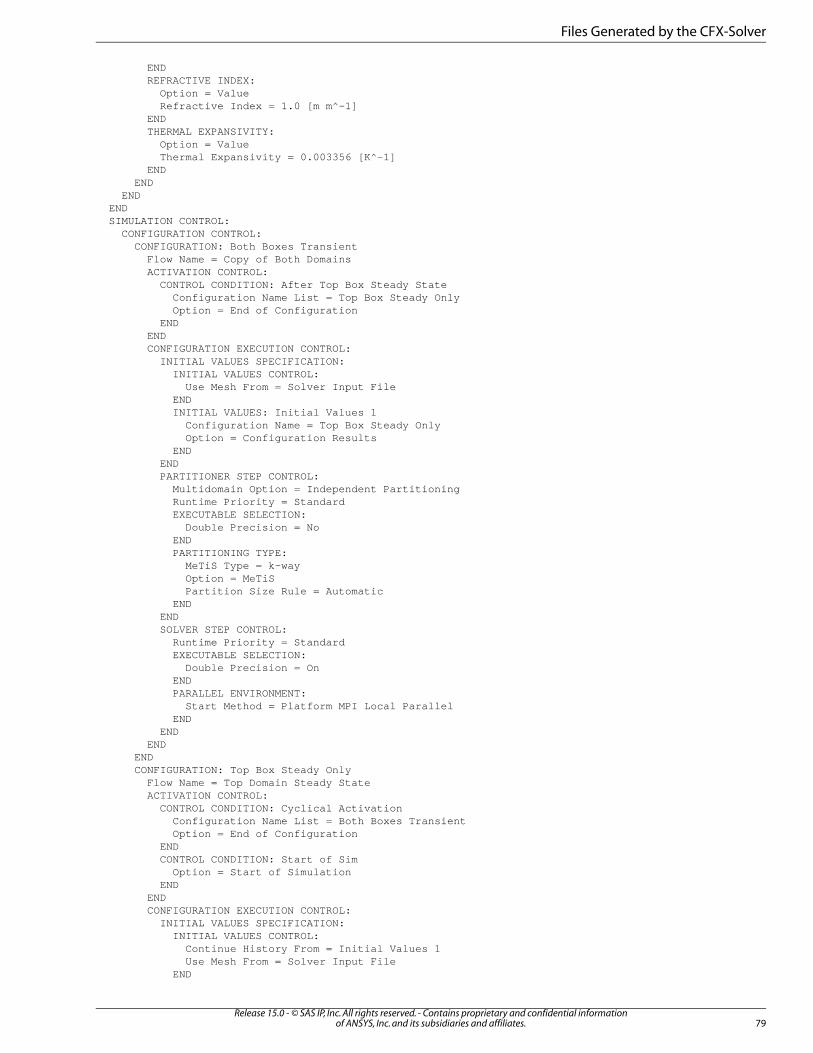
END REFRACTIVE INDEX: Option = Value Refractive Index = 1.0 [m m^-1] END THERMAL EXPANSIVITY: Option = Value Thermal Expansivity = 0.003356 [K^-1] END END END END SIMULATION CONTROL: CONFIGURATION CONTROL: CONFIGURATION: Both Boxes Transient Flow Name = Copy of Both Domains ACTIVATION CONTROL: CONTROL CONDITION: After Top Box Steady State Configuration Name List = Top Box Steady Only Option = End of Configuration END END CONFIGURATION EXECUTION CONTROL: INITIAL VALUES SPECIFICATION: INITIAL VALUES CONTROL: Use Mesh From = Solver Input File END INITIAL VALUES: Initial Values 1 Configuration Name = Top Box Steady Only Option = Configuration Results END END PARTITIONER STEP CONTROL: Multidomain Option = Independent Partitioning Runtime Priority = Standard EXECUTABLE SELECTION: Double Precision = No END PARTITIONING TYPE: MeTiS Type = k-way Option = MeTiS Partition Size Rule = Automatic END END SOLVER STEP CONTROL: Runtime Priority = Standard EXECUTABLE SELECTION: Double Precision = On END PARALLEL ENVIRONMENT: Start Method = Platform MPI Local Parallel END END END END CONFIGURATION: Top Box Steady Only Flow Name = Top Domain Steady State ACTIVATION CONTROL: CONTROL CONDITION: Cyclical Activation Configuration Name List = Both Boxes Transient Option = End of Configuration END CONTROL CONDITION: Start of Sim Option = Start of Simulation END END CONFIGURATION EXECUTION CONTROL: INITIAL VALUES SPECIFICATION: INITIAL VALUES CONTROL: Continue History From = Initial Values 1 Use Mesh From = Solver Input File END
79Release 15.0 - © SAS IP, Inc. All rights reserved. - Contains proprietary and confidential information
of ANSYS, Inc. and its subsidiaries and affiliates.
Files Generated by the CFX-Solver
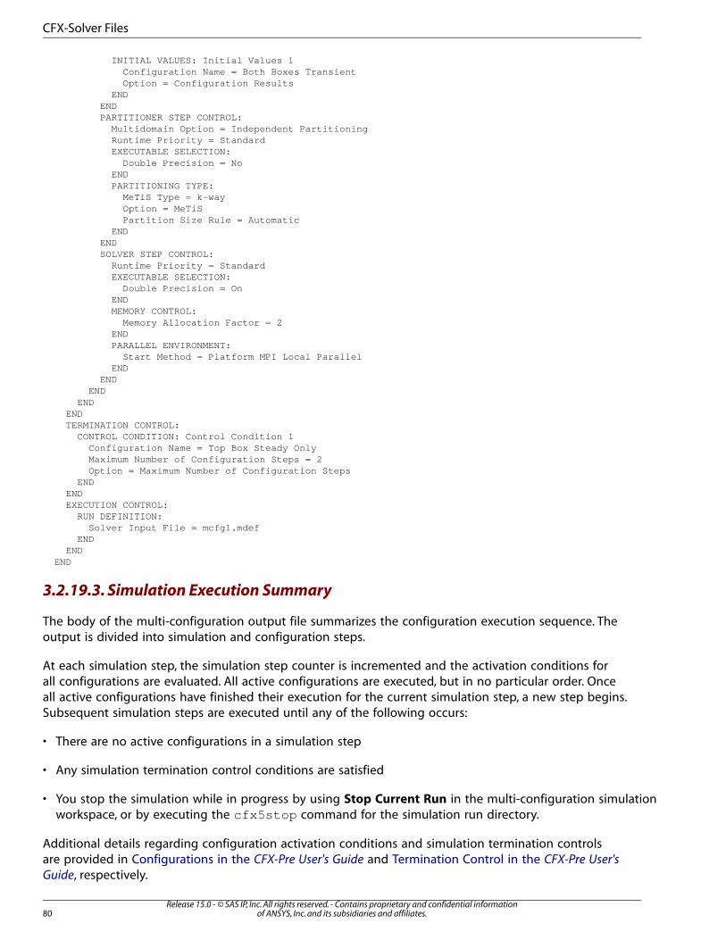
INITIAL VALUES: Initial Values 1 Configuration Name = Both Boxes Transient Option = Configuration Results END END PARTITIONER STEP CONTROL: Multidomain Option = Independent Partitioning Runtime Priority = Standard EXECUTABLE SELECTION: Double Precision = No END PARTITIONING TYPE: MeTiS Type = k-way Option = MeTiS Partition Size Rule = Automatic END END SOLVER STEP CONTROL: Runtime Priority = Standard EXECUTABLE SELECTION: Double Precision = On END MEMORY CONTROL: Memory Allocation Factor = 2 END PARALLEL ENVIRONMENT: Start Method = Platform MPI Local Parallel END END END END END TERMINATION CONTROL: CONTROL CONDITION: Control Condition 1 Configuration Name = Top Box Steady Only Maximum Number of Configuration Steps = 2 Option = Maximum Number of Configuration Steps END END EXECUTION CONTROL: RUN DEFINITION: Solver Input File = mcfg1.mdef END END END
3.2.19.3. Simulation Execution Summary
The body of the multi-configuration output file summarizes the configuration execution sequence. Theoutput is divided into simulation and configuration steps.
At each simulation step, the simulation step counter is incremented and the activation conditions forall configurations are evaluated. All active configurations are executed, but in no particular order. Onceall active configurations have finished their execution for the current simulation step, a new step begins.Subsequent simulation steps are executed until any of the following occurs:
• There are no active configurations in a simulation step
• Any simulation termination control conditions are satisfied
• You stop the simulation while in progress by using Stop Current Run in the multi-configuration simulationworkspace, or by executing the cfx5stop command for the simulation run directory.
Additional details regarding configuration activation conditions and simulation termination controlsare provided in Configurations in the CFX-Pre User's Guide and Termination Control in the CFX-Pre User's
Guide, respectively.
Release 15.0 - © SAS IP, Inc. All rights reserved. - Contains proprietary and confidential informationof ANSYS, Inc. and its subsidiaries and affiliates.80
CFX-Solver Files
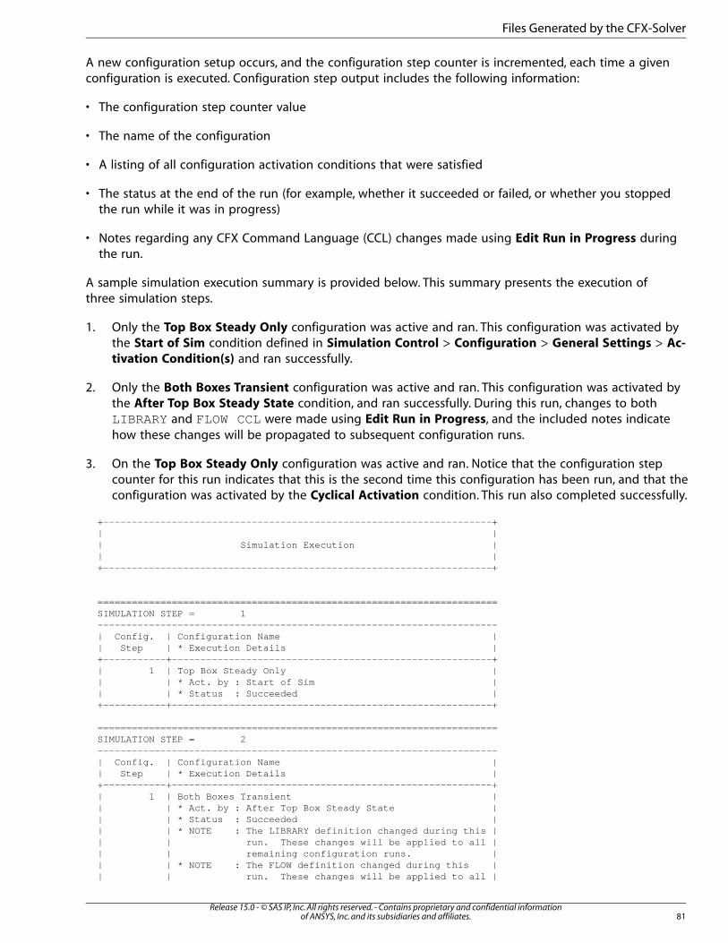
A new configuration setup occurs, and the configuration step counter is incremented, each time a givenconfiguration is executed. Configuration step output includes the following information:
• The configuration step counter value
• The name of the configuration
• A listing of all configuration activation conditions that were satisfied
• The status at the end of the run (for example, whether it succeeded or failed, or whether you stoppedthe run while it was in progress)
• Notes regarding any CFX Command Language (CCL) changes made using Edit Run in Progress duringthe run.
A sample simulation execution summary is provided below. This summary presents the execution ofthree simulation steps.
1. Only the Top Box Steady Only configuration was active and ran. This configuration was activated bythe Start of Sim condition defined in Simulation Control > Configuration > General Settings > Ac-
tivation Condition(s) and ran successfully.
2. Only the Both Boxes Transient configuration was active and ran. This configuration was activated bythe After Top Box Steady State condition, and ran successfully. During this run, changes to bothLIBRARY and FLOW CCL were made using Edit Run in Progress, and the included notes indicatehow these changes will be propagated to subsequent configuration runs.
3. On the Top Box Steady Only configuration was active and ran. Notice that the configuration stepcounter for this run indicates that this is the second time this configuration has been run, and that theconfiguration was activated by the Cyclical Activation condition. This run also completed successfully.
+--------------------------------------------------------------------+ | | | Simulation Execution | | | +--------------------------------------------------------------------+
====================================================================== SIMULATION STEP = 1 ---------------------------------------------------------------------- | Config. | Configuration Name | | Step | * Execution Details | +-----------+--------------------------------------------------------+ | 1 | Top Box Steady Only | | | * Act. by : Start of Sim | | | * Status : Succeeded | +-----------+--------------------------------------------------------+
====================================================================== SIMULATION STEP = 2 ---------------------------------------------------------------------- | Config. | Configuration Name | | Step | * Execution Details | +-----------+--------------------------------------------------------+ | 1 | Both Boxes Transient | | | * Act. by : After Top Box Steady State | | | * Status : Succeeded | | | * NOTE : The LIBRARY definition changed during this | | | run. These changes will be applied to all | | | remaining configuration runs. | | | * NOTE : The FLOW definition changed during this | | | run. These changes will be applied to all |
81Release 15.0 - © SAS IP, Inc. All rights reserved. - Contains proprietary and confidential information
of ANSYS, Inc. and its subsidiaries and affiliates.
Files Generated by the CFX-Solver

| | remaining runs of this configuration. | +-----------+--------------------------------------------------------+
====================================================================== SIMULATION STEP = 3 ---------------------------------------------------------------------- | Config. | Configuration Name | | Step | * Execution Details | +-----------+--------------------------------------------------------+ | 2 | Top Box Steady Only | | | * Act. by : Cyclical Activation | | | * Status : Succeeded | +-----------+--------------------------------------------------------+
3.2.19.4. Simulation Termination Condition Summary
This section of the multi-configuration output file identifies the reason(s) for terminating the simulation.In the example provided below, the user defined condition named Control Condition 1 was satisfied.For information regarding how this condition was defined, refer to the discussion in Termination Controlin the CFX-Pre User's Guide.
====================================================================== TERMINATION CONDITION SUMMARY ----------------------------------------------------------------------
* User: Control Condition 1
3.2.20. CFX Multi-Configuration Results File
The CFX-Solver will generate a results file with a name based on the CFX-Solver Input file. For example,running the CFX-Solver using the input file named file.mdef in a clean working directory will generatethe multi-configuration results file named file_001.mres .
For multi-configuration simulations, the CFX-Solver Input and CFX-Solver Results files are very similar;both are small files that contain only high level information about the simulation. In particular, theresults file contains:
• Global information about the simulation’s overall definition (such as Library CCL , configurationdefinitions and sequencing, etc…)
• Information about the configuration files (*.cfg , which contain configuration specific settings and meshes)
• Information about the CFX-Solver Results files (for details, see CFX-Solver Results File (p. 73)) generatedfor each configuration step.
CFX-Solver Output and CFX-Solver Results files for each configuration (and configuration step) executedare contained within the multi-configuration simulation’s run directory. For example, running the CFX-Solver using the input file named file.mdef in a clean working directory will generate a file anddirectory structure similar to the following:
• file_001.mres
• file_001.out
• file_001/
– Configuration1_001
– Configuration1_001.out
Release 15.0 - © SAS IP, Inc. All rights reserved. - Contains proprietary and confidential informationof ANSYS, Inc. and its subsidiaries and affiliates.82
CFX-Solver Files
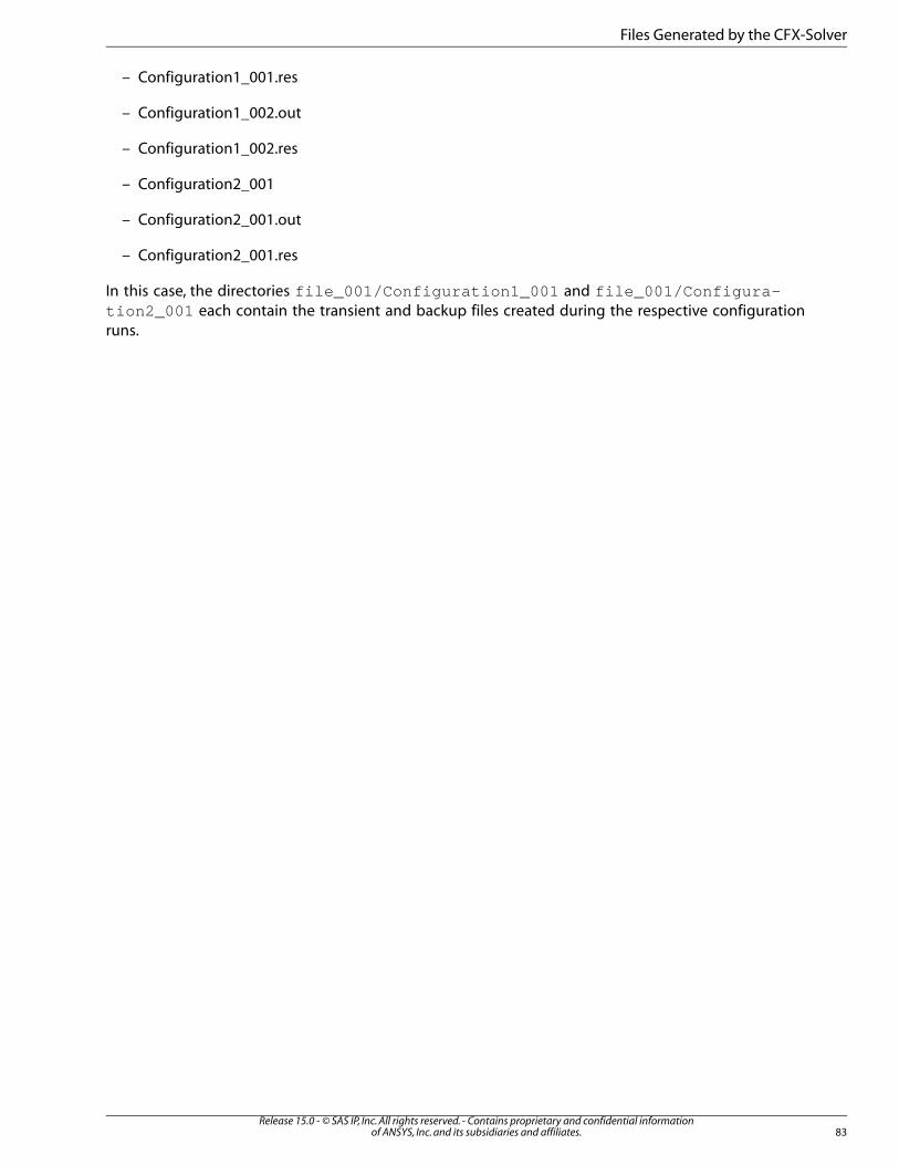
– Configuration1_001.res
– Configuration1_002.out
– Configuration1_002.res
– Configuration2_001
– Configuration2_001.out
– Configuration2_001.res
In this case, the directories file_001/Configuration1_001 and file_001/Configura-tion2_001 each contain the transient and backup files created during the respective configurationruns.
83Release 15.0 - © SAS IP, Inc. All rights reserved. - Contains proprietary and confidential information
of ANSYS, Inc. and its subsidiaries and affiliates.
Files Generated by the CFX-Solver

Release 15.0 - © SAS IP, Inc. All rights reserved. - Contains proprietary and confidential informationof ANSYS, Inc. and its subsidiaries and affiliates.84
Chapter 4: Residual Plotting
CFX-Solver calculates solutions to various equations. However, many cases result in residual values. Thisis due to an equation not being fully satisfied. Of course, if the solution is exact, then the residual iszero. However, because equation results only approximate physics, the results in a solution do not alwaysmatch reality.
This chapter describes:4.1. Equation Residual4.2. Convergence Results and RMS4.3.Transient Residual Plotting4.4. Residual Plotting for ANSYS Multi-field Runs
4.1. Equation Residual
CFX-Solver calculates the solution to various equations, given the appropriate boundary conditions andmodels for your particular CFD problem. For details, see Governing Equations in the CFX-Solver Theory
Guide.
At any stage of a calculation, each equation will not be satisfied exactly, and the “residual” of an equationidentifies how much the left-hand-side of the equation differs from the right-hand-side at any point inspace. If the solution is “exact,” then the residual is zero. This means that each of the relevant finitevolume equations is satisfied precisely. However, because these equations only model the physics ap-proximately, this does not mean that the solution exactly matches what happens in reality. If a solutionis converging, residuals should decrease with successive timesteps.
For example, assume that a given residual is 0.0005 kg s^-1. It is not obvious whether such a residualis large or small. For instance, if the problem involves flows such that about 0.5 kg flows into (and outof ) each mesh element every second, then a residual of 0.0005 kg s^-1 means the equation is satisfiedto within one part in a thousand, which is likely a reasonable solution. However, if the problem involvesflows of about 0.001 kg s^-1 into each mesh element, then the residual is nearly as large as the flow,and the solution is not good.
To make the scales of the residuals meaningful, the solver normalizes values by dividing the appropriatescales at each point. CFX-Solver Manager plots these normalized residuals using a log (base 10) scale.
The exact details of how the residuals are normalized are involved. For details, see Residual NormalizationProcedure in the CFX-Solver Theory Guide. However, it is useful to know that residuals are divided bythe solution range. If the linear solution diverges, this range may be very large and the normalized re-siduals would be meaningless.
4.2. Convergence Results and RMS
A measure of how well the solution is converged can be obtained by plotting the residuals for eachequation at the end of each timestep. A reasonably converged solution requires a maximum residuallevel no higher than 5.0E-4. Typically, the RMS (Root Mean Square) residual will be an order of magnitudelower than this.
85Release 15.0 - © SAS IP, Inc. All rights reserved. - Contains proprietary and confidential information
of ANSYS, Inc. and its subsidiaries and affiliates.
The RMS residual is obtained by taking all of the residuals throughout the domain, squaring them,taking the mean, and then taking the square root of the mean. This should present an idea of a typicalmagnitude of the residuals.
The Maximum Residuals and/or the RMS Residuals can be displayed in the convergence history plotsby selecting a specific monitor in Monitor Settings. For details, see Monitors Tab (p. 106).
The increase of a residual after any particular timestep does not imply that the solution is diverging. Itis usual for residuals to occasionally get larger, especially at the beginning of a run.
Note that even though convergence is good, there are still places where the residuals become largertemporarily.
It is also possible to have runs that do not converge at all, but simply deviate around the same values.
If the solution fails to converge, or convergence is happening very slowly, some tips on how to improvethe convergence are available. For details, see Monitoring and Obtaining Convergence in the CFX-Solver
Modeling Guide.
Tip
If you want to obtain residual plots for old runs, select File > Monitor Finished Run andselect a file to view.
4.3. Transient Residual Plotting
When monitoring a transient run with the plotting of coefficient loop data selected, CFX-Solver Manageroutputs the monitor data for each coefficient loop within each timestep. Each timestep is divided bythe number of inner coefficient loops. The values are produced for all variables in each coefficient loop.
With the plotting selected, CFX-Solver Manager outputs the graph of monitor data. The strategy thatCFX-Solver Manager uses for plot data is to plot the loops evenly across the space between iterationN-1 and N, so that the last coefficient loop is in line with iteration N on the plot. When the first coefficientloop value becomes available, it is the only value, and therefore it is placed in line with iteration N. Asmore data is added, the older coefficient loop values are shifted back, so that they are evenly spaced,with the last coefficient loop always in line with N.
Example: Assume that four coefficient loops were run for timestep 39. The first coefficient loop valuefor a plotted variable appears at position 38.25, the second at 38.5, the third at 38.75, and the fourthand final value is plotted at 39.
For details on plotting coefficient loop data, see Global Plot Settings Tab (p. 113).
4.4. Residual Plotting for ANSYS Multi-field Runs
The CFX-Solver Manager can be used to launch an ANSYS Multi-field Run. For such a run, it is not suffi-cient to consider only the convergence of CFX-Solver when deciding if results are converged: in addition,the convergence of CFX-Solver and the convergence of the data exchanged between the CFX and ANSYSSolvers must also be considered. The CFX-Solver Manager shows extra plots when monitoring an ANSYSMulti-field run to enable a graphical display of these extra convergence quantities.
For details, refer to the following sections:
Release 15.0 - © SAS IP, Inc. All rights reserved. - Contains proprietary and confidential informationof ANSYS, Inc. and its subsidiaries and affiliates.86
Residual Plotting
• Coupling CFX to an External Solver: ANSYS Multi-field Simulations in the CFX-Solver Modeling Guide
• ANSYS Field Solver Plots (p. 87)
• ANSYS Interface Loads Plots (p. 87)
For the extra plots to be displayed, the CFX-Solver Manager must have started CFX-Solver by selectingan MFX Run Mode of either Start ANSYS and CFX or Start ANSYS only (see MultiFieldTab (p. 12)), or CFX-Solver must have been started from the command line with the cfx5solvecommand. It is not possible for CFX-Solver Manager to display these plots if CFX-Solver was started bythe ANSYS CFX Launcher or from the command line directly.
4.4.1. ANSYS Field Solver Plots
These plots are only produced when the solid physics is set to use large displacements or when othernon-linear analyses are performed. It shows convergence information from CFX-Solver. Full details ofthe quantities plotted are described in Newton-Raphson Procedure in the Mechanical APDL Theory Ref-
erence.
In general, the CRIT quantities are the convergence criteria for each relevant variable. The L2/L1/INFquantities represent the L2 Norm/L1 Norm/Infinite Norm (respectively) of the relevant variable. TheCNVTOL command is used to specify a tolerance value applied when calculating the CRIT quantitiesand the desired norm. Note that the default is the L2 Norm if the ANSYS input file was produced byANSYS Mechanical. Convergence is realized when the desired norm is below the CRIT quantity.
The x-axis of the plot is the cumulative iteration number for ANSYS, which does not correspond totimesteps, coupling steps, or stagger iterations. Several ANSYS iterations will be performed for eachtimestep or coupling step, depending on how quickly ANSYS converges. You will usually see a somewhatspiky plot, as each quantity will be unconverged at the start of each time or coupling step, and thenconvergence will improve.
Several ANSYS Field Solver plots may be present, depending on the physics being solved within ANSYS.
4.4.2. ANSYS Interface Loads Plots
These plots show the convergence for each quantity that is part of the data exchanged between theCFX and ANSYS Solvers. There will always be two plots: ANSYS Interface Loads (Structural) and ANSYSInterface Loads (Thermal). The structural plot contains convergence information on forces and displace-ments, and the thermal plot contains information on temperature and heat flows/fluxes.
For each variable (each x-, y-, and z-component of the load is a separate variable), the convergencenorm for the data transferred across the interface is given by:
(4.1)∑
∑=
−�
� ���� ���
���
�
�
where represents the L2 norm of the transferred load, �� is the load component transferred at the
last stagger iteration, � ��� is the load component transferred at this stagger iteration, and the sum is
over all the individual load component values transferred (at different points in space). Each quantity
is considered to be converged when <� ���� , where ���� is the convergence target for that quantity
87Release 15.0 - © SAS IP, Inc. All rights reserved. - Contains proprietary and confidential information
of ANSYS, Inc. and its subsidiaries and affiliates.
Residual Plotting for ANSYS Multi-field Runs
set in CFX-Pre (see Solver Controls, External Coupling Tab in the CFX-Solver Modeling Guide) or directlyby the multi-field commands in the ANSYS input file (MFCO command).
Note
The definition of the convergence norm in Equation 4.1 (p. 87) was changed in Release12.0. To achieve convergence in Release 12.0 (and later) that is similar to that achievedprior to Release 12.0, set the new convergence target to be the square root of the con-vergence target used prior to Release 12.0. Furthermore, the default value for the con-vergence target in Release 12.0 was changed to 0.01.
Convergence of each quantity transferred across the interface is reported as �, where:
(4.2)=�� �
�
���
���
and this is the quantity plotted on the ANSYS Interface plots. This implies that each quantity has con-verged when the reported convergence reaches a negative value. In general, the ANSYS Interface Loads(Structural) plot will contain six lines, corresponding to three force components (FX, FY, and FZ) andthree displacements (UX, UY, and UZ), and the ANSYS Interface Loads (Thermal) plot will contain twolines (temperature and heat flow/flux). However, if the simulation is effectively 2D (only one elementacross), then forces and displacements in the third dimension are not exchanged and the correspondinglines will not be present.
The x-axis of the plot corresponds to the cumulative number of stagger iterations (coupling iterations)and there are several of these for every timestep. A “spiky” plot is expected as the quantities will notbe converged at the start of a timestep.
Release 15.0 - © SAS IP, Inc. All rights reserved. - Contains proprietary and confidential informationof ANSYS, Inc. and its subsidiaries and affiliates.88
Residual Plotting
Chapter 5: Editing CFX-Solver Input Files
This chapter discusses the details of editing existing CFX-Solver input (or results) files to make minorchanges to a CFD model, without having to use CFX-Pre:
5.1.Workflow Overview5.2. Command File Editor Overview5.3. Menus in the Command File Editor5.4. Command File Editor Rules5.5. Command File Editor Appearance5.6. Editing the Command Language (CCL) File5.7. Command Language File Rules5.8. RULES and VARIABLES Files
5.1. Workflow Overview
Modifications to CFX-Solver input (results) files can be performed using either the Command File Editorin CFX-Solver Manager or the cfx5cmds command from the command line, as shown in Figure 5.1: CFX-Solver Input File Modification Workflows (p. 89).
Figure 5.1: CFX-Solver Input File Modification Workflows
5.2. Command File Editor Overview
The simplest method of making changes to an existing CFX-Solver input file is to use the CommandFile Editor. The Command File Editor provides a tree-structured representation of a CFX-Solver inputfile. This enables modification of parameter settings and the addition of new parameters to existingCFX-Solver input files as required.
The Command File Editor can be invoked in multiple ways and each way provides a different function:
89Release 15.0 - © SAS IP, Inc. All rights reserved. - Contains proprietary and confidential information
of ANSYS, Inc. and its subsidiaries and affiliates.
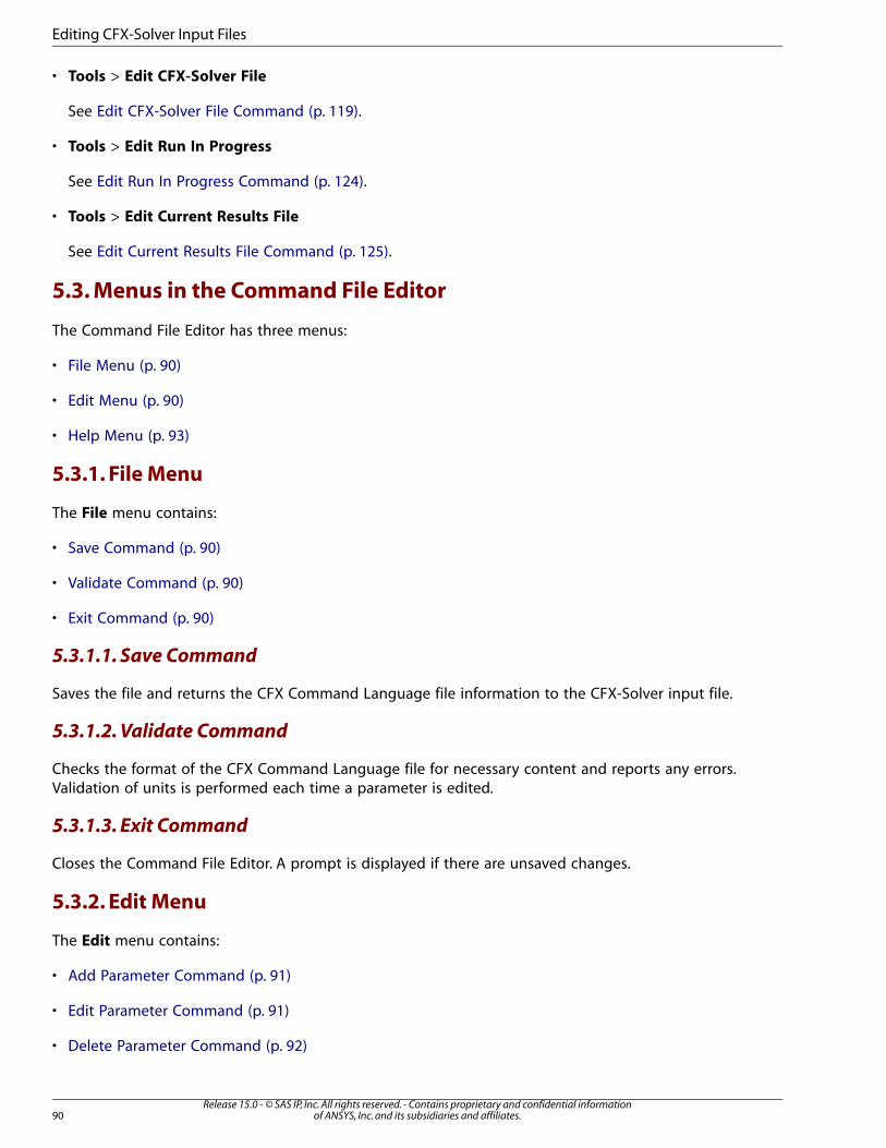
• Tools > Edit CFX-Solver File
See Edit CFX-Solver File Command (p. 119).
• Tools > Edit Run In Progress
See Edit Run In Progress Command (p. 124).
• Tools > Edit Current Results File
See Edit Current Results File Command (p. 125).
5.3. Menus in the Command File Editor
The Command File Editor has three menus:
• File Menu (p. 90)
• Edit Menu (p. 90)
• Help Menu (p. 93)
5.3.1. File Menu
The File menu contains:
• Save Command (p. 90)
• Validate Command (p. 90)
• Exit Command (p. 90)
5.3.1.1. Save Command
Saves the file and returns the CFX Command Language file information to the CFX-Solver input file.
5.3.1.2. Validate Command
Checks the format of the CFX Command Language file for necessary content and reports any errors.Validation of units is performed each time a parameter is edited.
5.3.1.3. Exit Command
Closes the Command File Editor. A prompt is displayed if there are unsaved changes.
5.3.2. Edit Menu
The Edit menu contains:
• Add Parameter Command (p. 91)
• Edit Parameter Command (p. 91)
• Delete Parameter Command (p. 92)
Release 15.0 - © SAS IP, Inc. All rights reserved. - Contains proprietary and confidential informationof ANSYS, Inc. and its subsidiaries and affiliates.90
Editing CFX-Solver Input Files
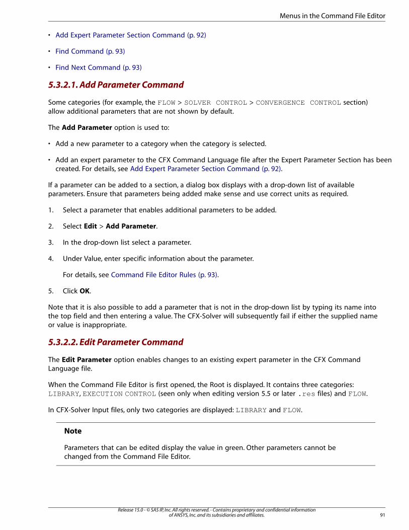
• Add Expert Parameter Section Command (p. 92)
• Find Command (p. 93)
• Find Next Command (p. 93)
5.3.2.1. Add Parameter Command
Some categories (for example, the FLOW > SOLVER CONTROL > CONVERGENCE CONTROL section)allow additional parameters that are not shown by default.
The Add Parameter option is used to:
• Add a new parameter to a category when the category is selected.
• Add an expert parameter to the CFX Command Language file after the Expert Parameter Section has beencreated. For details, see Add Expert Parameter Section Command (p. 92).
If a parameter can be added to a section, a dialog box displays with a drop-down list of availableparameters. Ensure that parameters being added make sense and use correct units as required.
1. Select a parameter that enables additional parameters to be added.
2. Select Edit > Add Parameter.
3. In the drop-down list select a parameter.
4. Under Value, enter specific information about the parameter.
For details, see Command File Editor Rules (p. 93).
5. Click OK.
Note that it is also possible to add a parameter that is not in the drop-down list by typing its name intothe top field and then entering a value. The CFX-Solver will subsequently fail if either the supplied nameor value is inappropriate.
5.3.2.2. Edit Parameter Command
The Edit Parameter option enables changes to an existing expert parameter in the CFX CommandLanguage file.
When the Command File Editor is first opened, the Root is displayed. It contains three categories:LIBRARY, EXECUTION CONTROL (seen only when editing version 5.5 or later .res files) and FLOW.
In CFX-Solver Input files, only two categories are displayed: LIBRARY and FLOW.
Note
Parameters that can be edited display the value in green. Other parameters cannot bechanged from the Command File Editor.
91Release 15.0 - © SAS IP, Inc. All rights reserved. - Contains proprietary and confidential information
of ANSYS, Inc. and its subsidiaries and affiliates.
Menus in the Command File Editor
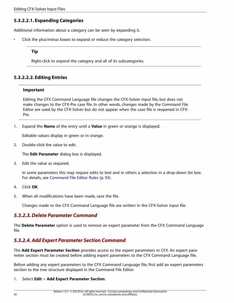
5.3.2.2.1. Expanding Categories
Additional information about a category can be seen by expanding it.
• Click the plus/minus boxes to expand or reduce the category selection.
Tip
Right-click to expand the category and all of its subcategories.
5.3.2.2.2. Editing Entries
Important
Editing the CFX Command Language file changes the CFX-Solver input file, but does notmake changes to the CFX-Pre case file. In other words, changes made by the Command FileEditor are used by the CFX-Solver but do not appear when the case file is reopened in CFX-Pre.
1. Expand the Name of the entry until a Value in green or orange is displayed.
Editable values display in green or in orange.
2. Double-click the value to edit.
The Edit Parameter dialog box is displayed.
3. Edit the value as required.
In some parameters this may require edits to text and in others a selection in a drop-down list box.For details, see Command File Editor Rules (p. 93).
4. Click OK.
5. When all modifications have been made, save the file.
Changes made to the CFX Command Language file are written in the CFX-Solver input file.
5.3.2.3. Delete Parameter Command
The Delete Parameter option is used to remove an expert parameter from the CFX Command Languagefile.
5.3.2.4. Add Expert Parameter Section Command
The Add Expert Parameter Section provides access to the expert parameters in CFX. An expert para-meter section must be created before adding expert parameters to the CFX Command Language file.
Before adding any expert parameters to the CFX Command Language file, first add an expert parameterssection to the tree structure displayed in the Command File Editor.
1. Select Edit > Add Expert Parameter Section.
Release 15.0 - © SAS IP, Inc. All rights reserved. - Contains proprietary and confidential informationof ANSYS, Inc. and its subsidiaries and affiliates.92
Editing CFX-Solver Input Files
The EXPERT PARAMETERS: section is added to the bottom of the FLOW branch of the tree.
2. Expand FLOW.
3. Select EXPERT PARAMETERS.
4. Add parameters as required.
For details, see Add Parameter Command (p. 91).
Once the value for an expert parameter has been set, it can be edited as needed. For details, see EditParameter Command (p. 91).
5.3.2.5. Find Command
Enables searching of the CFX Command Language file for a keyword or keywords.
5.3.2.6. Find Next Command
Finds the next occurrence of the keyword or keywords.
5.3.3. Help Menu
The Help menu contains:
• Help On Command File Editor Command (p. 93)
• Help On Expert Parameters Command (p. 93)
5.3.3.1. On Command File Editor Command
The help associated with the Command File Editor is launched.
5.3.3.2. On Expert Parameters Command
The CFX-Solver Expert Control Parameters help is launched.
5.4. Command File Editor Rules
If you are unsure about which values are appropriate to enter, select Help > On Expert Parameters
from the main Command File Editor window to view a description and valid values for the parameters.
The following rules apply when using the Command File Editor:
• Everything is case-sensitive. Use care to distinguish upper case letters from lower case letters.
• Parameter names must start with a letter (not a number or symbol). Subsequent characters can be letters,numbers, spaces or tabs.
• Spaces appearing before or after a name are not considered to be part of the name.
• Multiple spaces and tabs appearing inside a name are treated as a single space.
• For parameters requiring a logical value, enter T or t for true, and F or f for false. For many parametersrequiring an integer value only a few integer values are valid.
93Release 15.0 - © SAS IP, Inc. All rights reserved. - Contains proprietary and confidential information
of ANSYS, Inc. and its subsidiaries and affiliates.
Command File Editor Rules
These rules should suffice for simple editing operations. To perform more complicated editing operations,consider editing the command file directly. For details, see Editing the Command Language (CCL)File (p. 94).
5.5. Command File Editor Appearance
Some of the file information under the Name and Value headings may be truncated when the treestructure is expanded. The amount of space allocated to the name or the value can be configured.
1. Position the mouse cursor between the Name and Value headings.
That is, place the cursor over the line that separates the two headings. The cursor appears as adouble line with an arrow to the left and the right.
2. Click and drag to expand or contract the width of the column.
For lengthy lines (such as those that contain lists), double-click the line. This opens the line in aconfigurable dialog box for viewing and editing.
5.6. Editing the Command Language (CCL) File
In some circumstances, more significant changes may be required to the CFX-Solver input file than ispossible through the Command File Editor. ANSYS CFX allows the use of a text editor to edit the CFXCommand Language file.
Note
This feature is for expert users only. Extreme care must be taken when editing a CFX CommandLanguage file. Changes made to the CFX Command Language file are reflected in the CFX-Solver input file and may have negative effects on the model. It is strongly advised that ori-ginal files are backed up before edits are made to them.
To generate the CFX Command Language file, use the cfx5cmds command in a UNIX terminal or aWindows command line that is set up correctly to run CFX commands. For details, see Command Linein the CFX Reference Guide.
5.7. Command Language File Rules
The following rules apply when using a text editor to change a CFX Command Language file:
• Changing the solution units outside of CFX-Pre is not recommended. For details, see Setting the SolutionUnits in the CFX-Pre User's Guide.
• Everything apart from expert parameter names is case-sensitive. Use care to distinguish upper case lettersfrom lowercase letters. You should use lowercase letters for expert parameter names to match thoseshown in the Command File Editor Help's Expert Parameters section.
• The name of any variable must start with a letter (not a number or symbol). Subsequent characters canbe letters, numbers, spaces, or tabs.
• Spaces appearing before or after a name are not considered to be part of the name.
• Multiple spaces and tabs appearing inside a name are treated as a single space.
Release 15.0 - © SAS IP, Inc. All rights reserved. - Contains proprietary and confidential informationof ANSYS, Inc. and its subsidiaries and affiliates.94
Editing CFX-Solver Input Files
• Nothing is sensitive to indentation. Indentation is used only to make the appearance of the text clearer.
• The comment character is the pound, or number sign (#). Anything appearing to the right of this characteris ignored. For instance:
PARAMETER = 3.2 # This text is ignored
• The line continuation character is the backslash (\ ). To break a long line of text into two or more lines,insert a backslash character at the end of the first line. For instance, both of the following declarationsare handled the same way:
NAME = default temperature used in the first simulationNAME = default temperature used \ in the first simulation
• A line containing CFX Expression Language must be no more than 256 characters long. Other lines canbe of any length.
The RULES and VARIABLES files can be a useful guide when editing a CCL file. For details, see RULESand VARIABLES Files (p. 96).
Some objects in the CCL file can be defined with a default value and then overridden by local values.For example, the SOLVER CONTROL section of a CCL file may look like:
SOLVER CONTROL : CONVERGENCE CONTROL : Maximum Number of Iterations = 100 Timescale Control = Physical Timescale Physical Timescale = 5.E-1 [s] END EQUATION CLASS : momentum CONVERGENCE CONTROL : Timescale Control = Physical Timescale Physical Timescale = 1.E-1 [s] END END CONVERGENCE CRITERIA : Residual Type = RMS Residual Target = 1.E-4 END ADVECTION SCHEME : Option = Upwind END DYNAMIC MODEL CONTROL : Global Dynamic Model Control = No ENDEND
The first CONVERGENCE CONTROL object defines values that apply to all equation classes. The physicaltime scale is then locally overridden for the momentum equation class. Other objects, including theADVECTION SCHEME, can be locally overridden in the same way. The order in which objects appearis not important, so an object can be assigned an override before its default has been set. Only someparameters may be set to a different local value; for example, it does not make sense to set the MaximumNumber of Iterations locally.
95Release 15.0 - © SAS IP, Inc. All rights reserved. - Contains proprietary and confidential information
of ANSYS, Inc. and its subsidiaries and affiliates.
Command Language File Rules
5.8. RULES and VARIABLES Files
The RULES and VARIABLES files can be useful when editing a CCL file. They provide information onvalid options, variables, and dependencies. Both files are located in <CFXROOT>/etc/ and can beviewed in any text editor.
Note
In some cases, the RULES and VARIABLES files contain information about variables, para-meters, models and options that are not yet fully supported in the CFX-Solver. Use cautionwith features that are not documented elsewhere as these may cause the CFX-Solver to failor produce invalid results.
5.8.1. VARIABLES File
The VARIABLES file lists all the variables available in the CFX-Solver. Information provided for eachvariable appears similar to the following:
VARIABLE: vel Option = Definition MMS Name = VEL Long Name = Velocity Tensor Type = VECTOR Quantity = Velocity Status = P User Level = 1 Output to Jobfile = No Output to Postprocessor = Yes Component Short Names = \ u, \ v, \ w Component Long Names = \ Velocity u, \ Velocity v, \ Velocity w Component MMS Names = \ VEL-1, \ VEL-2, \ VEL-3 General Availability = ADAPTION, RESULTS, CEL Variable Description = Velocity Variable Scope = PHASEEND
The following information can be identified:
• The name appearing immediately after VARIABLE: (in this case vel ) is the CFX-Solver name or shortname for the variable.
• For scalar quantities (Tensor Type = SCALAR ), the name appearing after VARIABLE: is the namethat must be used in any CEL expressions. The MMS Name and Long Name are not valid names to usefor this purpose.
• For vector and tensor quantities (Tensor Type = VECTOR and Tensor Type = SYMTEN2 ), theComponent Short Names (u, v and w in this case) are names that must be used in any CEL expressions.
Release 15.0 - © SAS IP, Inc. All rights reserved. - Contains proprietary and confidential informationof ANSYS, Inc. and its subsidiaries and affiliates.96
Editing CFX-Solver Input Files
• The User Level setting controls when the variable is seen. Variables of User Level = 1 will appearin drop-down variable selection menus in CFD-Post. Variables with User Level = 2 orUser Level = 3 will only appear in the full list of variables.
• The Output to Postprocessor setting controls if the variable is written to the results file for usein CFD-Post. A variable must be involved in the simulation before is has the potential to be written out.
• The General Availability field determines when a variable can be used. Only variables whoseGeneral Availability includes CEL can be used in CEL expressions.
• The names of all VARIABLE, EQUATION DEFINITION and FUNCTION objects are reserved names.These names should not be used as the name for any CEL expressions, Additional Variables, user routines,or user functions, and so on.
The end of the VARIABLES file contains a section listing call back definitions. Using call backs that arenot documented, or using them on locations other than those documented, will produce invalid results.For details, see Quantitative Function List in the CFX Reference Guide.
5.8.2. RULES File
The RULES file contains information about which models and parameters are valid options. This includesSINGLETON, OBJECT and PARAMETER items.
5.8.2.1. RULES
The first items in the RULES file list the top level SINGLETON objects. All other items are children ofthese optional top level objects.
• RULES: This could be used to modify the list of allowed options. This should always be done locally.
• LIBRARY: Includes libraries for materials, reactions, CEL and user routines. Add new materials and reactionsusing a local library.
• FLOW: Contains the current problem definition.
• USER: Where user parameters may be stored for later retrieval through User Fortran.
• COMMAND FILE: Contains the command file version number.
• EXECUTION CONTROL: Contains information about the parallel setup and other settings controlled inthe CFX-Solver Manager.
Details about models that are not available can also be found through the user interface. For example,the SINGLETON: ADVECTION SCHEME item includes the QUICK scheme.
5.8.2.2. SINGLETON
A SINGLETON object is permitted to appear once as the child of a parent object. For this reasonSINGLETON objects do not have names associated with them, for example:
LIBRARY : CEL : EXPRESSIONS :
97Release 15.0 - © SAS IP, Inc. All rights reserved. - Contains proprietary and confidential information
of ANSYS, Inc. and its subsidiaries and affiliates.
RULES and VARIABLES Files
Each of these three items is a SINGLETON object. The LIBRARY SINGLETON may only have one CELSINGLETON, and the CEL SINGLETON may only have one EXPRESSIONS SINGLETON. Parametersand child definitions do not need to be grouped for a SINGLETON into a single location; this is doneautomatically by the CFX-Solver. For example, the following is valid:
LIBRARY : CEL : EXPRESSIONS : myexp1 = 1 [ m ] END ENDEND...LIBRARY : CEL : EXPRESSIONS : myexp2 = 2 [ m ] END ENDEND
5.8.2.3. OBJECT
An OBJECT is similar to a SINGLETON except that more than one can appear as the child of a parentobject. For this reason each OBJECT must have a name, for example:
FLOW : DOMAIN : domain1 ... END DOMAIN : domain2 ... ENDEND
Two OBJECT items of type DOMAIN have been defined with names domain1 and domain2 . Theseare children of the FLOW SINGLETON.
5.8.2.4. PARAMETER
A PARAMETER consists of a name, followed by the “=” character, followed by a value. Many parametersin the RULES file cannot be set in a CCL file and therefore cannot be altered.
• The Parameter Type tells you the type of values the parameter is allowed to take. It could be Real ,Real List , Integer , Integer List , String or String List . When a list is valid, items shouldbe comma separated.
• Some parameters contain an Allowed String List . This contains valid strings that can be used forthat parameter.
• Each PARAMETER that you can set has a Dependency List that lists the variables the PARAMETERcan depend upon. XYZ refers to the x, y and z coordinates. XYZT refers to the x, y and z coordinates andtime. The CCL file can be edited based on the dependencies listed here.
• If a PARAMETER contains the item Dynamic Reread Item = Yes , then it can be modified while arun is in progress. Some SINGLETON objects also contain this item. For details, see Edit Run In ProgressCommand (p. 124).
Release 15.0 - © SAS IP, Inc. All rights reserved. - Contains proprietary and confidential informationof ANSYS, Inc. and its subsidiaries and affiliates.98
Editing CFX-Solver Input Files
Chapter 6: CFX-Solver Manager File Menu
This chapter describes the commands available from the CFX-Solver File menu:
Define Run Command
Running the CFX-Solver involves passing it the geometry, models, boundary conditions, and start-upinformation that it needs to calculate a solution to your CFD problem. The Define Run form is whereyou specify the information which is passed to the CFX-Solver. Some runs of the CFX-Solver require youto specify only the name of the CFX-Solver input file; others also require the name of an initial valuesfile. Extra tabs become available when Show Advanced Controls is selected. For details, see The DefineRun Dialog Box (p. 10).
Monitor Run in Progress Command
Used when CFX-Solver Manager has been closed and a run currently underway in the Solver must bedisplayed.
1. Select File > Monitor Run in Progress.
The Select a Run Directory (.dir) dialog box is displayed.
2. Browse to the directory containing the current run.
3. Select the current run.
4. Click OK.
Data up to the current timestep is loaded.
Monitor Finished Run Command
Used to view the residual plots of a finished run.
1. Select File > Monitor Finished Run.
The Monitor Finished Run dialog box is displayed.
2. Under File Type, select the type of files to view.
3. Browse to the directory containing the finished run.
4. Select the run to view.
If required, select a different file.
5. Click OK.
The data is loaded.
99Release 15.0 - © SAS IP, Inc. All rights reserved. - Contains proprietary and confidential information
of ANSYS, Inc. and its subsidiaries and affiliates.
Close Workspace Command
Closes all windows related to the current run. Any other runs that were open are not affected, and thelast open run prior to the current run is displayed. If the Solver was in progress on the current run, itcontinues to operate in the background. The run can be re-monitored; see Monitor Run in ProgressCommand (p. 99) or Monitor Finished Run Command (p. 99), as appropriate.
Quit Command
To quit CFX-Solver Manager, select File > Quit. Closing CFX-Solver Manager does not stop CFX-Solverjobs that are currently running. CFX-Solver Manager can be re-opened to take control of these jobsagain simply by opening CFX-Solver Manager and selecting Monitor Run in Progress. For details, seeMonitor Run in Progress Command (p. 99).
Release 15.0 - © SAS IP, Inc. All rights reserved. - Contains proprietary and confidential informationof ANSYS, Inc. and its subsidiaries and affiliates.100
CFX-Solver Manager File Menu
Chapter 7: CFX-Solver Manager Edit Menu
The Edit > Options dialog box enables you to set various general preferences. Settings are retainedper user.
1. Select Edit > Options.
The Options dialog box appears.
2. Set options as required. For descriptions of the available options, see:
• CFX-Solver Manager Options (p. 101)
• Common Options (p. 102)
If desired, you can use the CFX Defaults or the Workbench Defaults buttons at the bottom ofthe dialog box to quickly set CFX-Pre, CFX-Solver Manager, and CFD-Post to have the standardoperation of CFX or Workbench respectively. The only settings visible in CFX-Solver Manager thatare affected by these buttons are Common > Viewer Setup > Mouse Mapping.
3. Click OK.
7.1. CFX-Solver Manager Options
When the Options dialog box appears, CFX-Solver Manager options can be set under SolverManager.
Default Layout Mode
You may specify a default layout mode to specify what mode monitors are presented when starting anew run. Select from the following:
• Multiple Windows
• Tabbed
Show Original Variable Names
If selected, the variable names will be shown with their original names. By default, this option is notselected and is generally left at that default setting.
Don’t write Backup file on Edit Run In Progress
By default, a backup file is written. For details, see Edit Run In Progress Command (p. 124).
101Release 15.0 - © SAS IP, Inc. All rights reserved. - Contains proprietary and confidential information
of ANSYS, Inc. and its subsidiaries and affiliates.
Save Workspace to Results File
By default, this option is selected, enabling the CFX-Solver Manager workspace state to be saved auto-matically into the results file for the run. This means that if you subsequently re-monitor the run, anycustom plots or plot settings that you used for the original run will be preserved.
Note that with this option selected, opening any ANSYS CFX results file in Release 11.0 or later of theCFX-Solver Manager will modify the results file in such a way that it becomes incompatible with Release10.0 or earlier of the CFX-Solver Manager. In general, compatibility cannot be guaranteed whenever anANSYS CFX results file from a particular release is opened in a CFX-Solver Manager from a later release.The results file will still be functional for the CFX-Solver from the earlier release, but you will not beable to monitor such a run using the CFX-Solver Manager from the earlier release. You should, therefore,disable Save Workspace to Results File when switching back and forth between different releases ofthe CFX-Solver Manager. You should also disable this option if you want to retain an unmodified resultsfile.
Enable Beta Features
Some beta features are hidden in the user interface. You can select this option to “unhide” those betafeatures. When selected, such Beta features will be identified by "(Beta)" in the user interface.
Monitor
Multiple options exist that can be monitored as required.
• The visibility for each type of residual can be toggled on or off. Settings take effect the next time a runis started, or the next time a results file is viewed.
• If visibility is disabled for all residuals in a plot monitor, the monitor will not be created.
Monitor options are available to specify global residual display preferences. Settings chosen on theform apply for all future solver runs and override default display settings for monitors. Monitors canstill be created using the Workspace menu. For details, see New Monitor Command (p. 114).
7.2. Common Options
Auto Save
Select the time between automatic saves.
To turn off automatic saves, set Auto Save to Never .
Note
This option affects more than one CFX product.
Temporary directory
To set a temporary directory, click Browse to find a convenient directory where the autosave feature
will save state files.
Release 15.0 - © SAS IP, Inc. All rights reserved. - Contains proprietary and confidential informationof ANSYS, Inc. and its subsidiaries and affiliates.102
CFX-Solver Manager Edit Menu
7.2.1. Appearance
The appearance of the user interface can be controlled from the Appearance options. The default userinterface style will be set to that of your machine. For example, on Windows, the user interface has aWindows look to it. If, for example, a Motif appearance to the user interface is preferred, select to usethis instead of the Windows style.
1. Under GUI Style, select the user interface style to use.
2. For Font and Formatted Font, specify the fonts to use in the application.
Note
It is important not to set the font size too high (over 24 pt. is not recommended) or thedialog boxes may become difficult to read. Setting the font size too small may causesome portions of the text to not be visible on monitors set at low resolutions. It is alsoimportant not to set the font to a family such as Webdings, Wingdings, Symbols, orsimilar type faces, or the dialog boxes become illegible.
Note
Formatted Font affects only the font used in CFX-Solver Manager for the out file display.
7.2.2. Viewer Setup
1. Select Double Buffering to use two color buffers for improved visualization.
For details, see Double Buffering (p. 103).
2. Select or clear Unlimited Zoom.
For details, see Unlimited Zoom (p. 103).
7.2.2.1. Double Buffering
Double Buffering is a feature supported by most OpenGL implementations. It provides two completecolor buffers that swap between each other to animate graphics smoothly. If your implementation ofOpenGL does not support double buffering, you can clear this check box.
7.2.2.2. Unlimited Zoom
By default, zoom is restricted to prevent graphics problems related to depth sorting. Selecting Unlimited
Zoom allows an unrestricted zoom.
7.2.2.3. Mouse Mapping
The mouse-mapping options allow you to assign viewer actions to mouse clicks and keyboard/mousecombinations. These options are available when running in stand-alone mode. To adjust or view themouse mapping options, select Edit > Options, then Viewer Setup > Mouse Mapping. For details,see Mouse Button Mapping.
103Release 15.0 - © SAS IP, Inc. All rights reserved. - Contains proprietary and confidential information
of ANSYS, Inc. and its subsidiaries and affiliates.
Common Options

7.2.3. Units
1. Under System, select the unit system to use. Unit systems are sets of quantity types for mass, length,time, and so on.
The options under System include SI , CGS, English Engineering , British Technical ,US Customary , US Engineering , or Custom . Only Custom enables you to redefine aquantity type (for example, to use inches for the dimensions in a file that otherwise used SI units).
The most common quantity types appear in the main Options dialog box; to see all quantity types,click More Units.
2. Select or clear Always convert units to Preferred Units.
If Always convert units to Preferred Units is selected, the units of entered quantities are imme-diately converted to those set in this dialog box.
For example, if you have set Velocity to [m s^-1] in this dialog box to make that the preferredvelocity unit, and elsewhere you enter 20 [mile hr^-1] for a velocity quantity, the enteredvalue is immediately converted and displayed as 8.94078 [m s^-1] .
Release 15.0 - © SAS IP, Inc. All rights reserved. - Contains proprietary and confidential informationof ANSYS, Inc. and its subsidiaries and affiliates.104
CFX-Solver Manager Edit Menu
Chapter 8: CFX-Solver Manager Workspace Menu
The Workspace menu controls layout, plots, and text windows that are visible in the viewer. With theWorkspace menu you can:
• Back up, restart, or stop the current run
• Change the properties for the current workspace
• Create new monitors for simulations
• Switch between multiple windows and tabbed layout (using the Toggle Layout menu option)
• Switch between viewing RMS and Maximum residual values at any time during or after a run.
This chapter describes the commands available from the Workspace menu:8.1.Workspace Properties Command8.2. New Monitor Command8.3. Stop Current Run Command8.4. Restart Current Run Command8.5. Backup Run Command8.6. Arrange Workspace Command8.7.Toggle Layout Type Command8.8. Load Layout Command8.9. Save Layout Command8.10.View RMS Residuals Command8.11.View MAX Residuals Command8.12. Reset to Default Workspace Command8.13. Close Workspace Command
8.1. Workspace Properties Command
When loading a results file or starting a solver run, CFX-Solver Manager checks the type of run in orderto create the correct plots. For example, a volume fraction plot will be created for multiphase simulations.
By default, appropriate monitors are automatically created by CFX-Solver Manager for the particulartype of simulation you are running. However, the type and/or number of plots that appear can bechanged by using Workspace > Workspace Properties. This launches the Workspace Properties
dialog box, which has the following tabs:
• General Settings Tab (p. 106)
• Monitors Tab (p. 106)
• Global Plot Settings Tab (p. 113)
105Release 15.0 - © SAS IP, Inc. All rights reserved. - Contains proprietary and confidential information
of ANSYS, Inc. and its subsidiaries and affiliates.
8.1.1. General Settings Tab
The General Settings tab displays the following workspace information, which cannot be edited.
• Out File displays the path and name of the CFX-Solver Output file for the run displayed in CFX-SolverManager.
• Directory displays the path and name of the directory for the run displayed in CFX-Solver Manager.
The locations can be set in the Working Directory option when defining the run. For additional inform-ation, see Define Run Command (p. 99) and Run Definition Tab (p. 10). Information on selecting differentruns is available in Workspace Selector (p. 2).
8.1.2. Monitors Tab
Not all of the monitors relevant to a solution are displayed by default; however, you can add them inthe Monitors tab. The following types of monitors are available:
• Plot Monitor (p. 106)
• Residual Monitor (p. 106)
• Text Monitor (p. 106)
8.1.2.1. Plot Monitor
Plot monitors show the values of expressions versus timestep.
8.1.2.2. Residual Monitor
Residual monitors show the values of residuals for equation variables versus timestep.
8.1.2.3. Text Monitor
Text monitors show the contents of text files that are updated as the run proceeds.
8.1.2.4. Filter Selector
The Filter selector is a drop-down list that shows the monitor types available in CFX-Solver Manager.Use this selector to control the monitors displayed under the Monitors tab. The All setting displaysthe full list of available monitors.
8.1.3. Creating Monitors
Monitors can be created within Workspace Properties. However, they can also be created directly fromthe Workspace menu by selecting New Monitor.
1. Select Workspace > Workspace Properties.
2. Select Monitors.
3. Click New .
Release 15.0 - © SAS IP, Inc. All rights reserved. - Contains proprietary and confidential informationof ANSYS, Inc. and its subsidiaries and affiliates.106
CFX-Solver Manager Workspace Menu

The New Monitor dialog box is displayed.
4. Under Name, type the name of the new monitor.
5. Under Type, select Plot Monitor , Residual Monitor or Text Monitor .
6. Click OK.
The Monitor Properties dialog box is displayed.
7. Configure the monitor as required.
• General Settings Tab (p. 108)
• Range Settings Tab (p. 108)
• Plot Lines Tab (p. 109)
8.1.4. Modifying Monitors
1. Select Workspace > Workspace Properties.
2. Select Monitors.
3. Select the monitor to modify.
4. Click Edit .
The Monitor Properties dialog box is displayed.
5. Configure the monitor as required.
• General Settings Tab (p. 108)
• Range Settings Tab (p. 108)
• Plot Lines Tab (p. 109)
Note
Alternatively, to access the Monitor Properties dialog box, right-click the graph area of anyof the monitor tabs.
8.1.4.1. Deleting Monitors
1. Select Workspace > Workspace Properties.
2. Select Monitors.
3. Select the monitor to delete.
4. Click Delete .
107Release 15.0 - © SAS IP, Inc. All rights reserved. - Contains proprietary and confidential information
of ANSYS, Inc. and its subsidiaries and affiliates.
Workspace Properties Command
8.1.4.2. Monitor Properties
Monitor properties differ depending on the type of monitor. Up to three tabs are available to configuremonitor properties:
• General Settings Tab (p. 108)
• Range Settings Tab (p. 108)
• Plot Lines Tab (p. 109)
8.1.4.2.1. General Settings Tab
1. Under Window Label, type the name to display for the monitor.
2. If working with a text monitor:
a. Under Text File Name, click Browse and select a file containing the definition for the text
monitor.
This can be any .out file.
b. Select or clear Disable this Monitor.
If selected, the monitor is disabled.
3. If working with a plot monitor or a residual monitor:
a. Under Background Color, click Color Selector and set the background color.
b. Select or clear Display Legend.
If selected, the legend is displayed in the monitor.
c. Under Grid Mode select Both , X, Y or None.
This determines if grid lines appear along the X or Y axis, on both or not at all.
d. Under Grid Color, click Color Selector and set the grid color.
4. Select or clear Visibility.
If selected, the monitor is displayed.
8.1.4.2.2. Range Settings Tab
1. Under Timestep Range Mode, select from the following options:
• Display All displays values for every iteration. If viewing a restarted run, results from the previousrun are also visible.
• Most Recent displays the current iteration and a number of previous iterations.
Release 15.0 - © SAS IP, Inc. All rights reserved. - Contains proprietary and confidential informationof ANSYS, Inc. and its subsidiaries and affiliates.108
CFX-Solver Manager Workspace Menu
• Fixed displays a beginning and end iteration that is always displayed, regardless of the current iter-ation number.
• This Run Only displays the range for the current run. If the run is a restart, previous runs are notincluded in the range.
• This Run and Previous Timestep displays all timesteps for the current run and the lasttimestep from any previous run. By selecting this option, plots will contain all data generated in thecurrent run and will also display the coefficient loop data for the previous timestep from any previousrun from which the current run was started.
2. Under Variable Axis, select or clear Use Logarithmic Scale.
If selected, Set Manual Scale (Log) is automatically selected.
3. Under Set Manual Scale (Log) or Set Manual Scale (Linear) set the Upper Bound and Lower Bound
values for the variable axis.
Note
If you accidentally specify a lower bound that is higher than the upper bound, CFX-Solver Manager will reverse the values internally to determine the range, but the valuesyou entered will not be changed in the user interface.
4. Complete the timestep configuration based on the Timestep Range Option selected.
• Most Recent requires a value for Timestep Window Size.
• Fixed requires values for First Timestep and Last Timestep.
8.1.4.2.3. Plot Lines Tab
Variables that are available to plot can come from a variety of sources. Select the source by settingVariable Set appropriately. Available settings are:
• CFX Solver: This option will be available for all CFX runs, and enables the specification of all variablesrelating to the CFX run.
• ANSYS Field Solver: This option is available only if an ANSYS Multi-field run is being performed withANSYS running a nonlinear simulation, and enables the selection of ANSYS convergence variables.
• ANSYS Interface Loads: This option is only available if an ANSYS Multi-field run is being performed, andenables the selection of the variables relating to the data exchanged between the ANSYS and CFX Solvers.
Plot lines can be displayed as required:
1. Expand a plot line variable by clicking + next to it.
Categories are displayed.
2. Expand a category by clicking + next to it.
109Release 15.0 - © SAS IP, Inc. All rights reserved. - Contains proprietary and confidential information
of ANSYS, Inc. and its subsidiaries and affiliates.
Workspace Properties Command
3. Select or clear specific plot line variables.
4. If working with a Residual Monitor, under Residual Mode, select RMS or MAX.
Residual Mode acts as a visibility filter for variables of Residual type selected by default. If a variableof type Residual is not selected by default it is plotted even if its type does not match the ResidualMode setting.
5. Click Apply.
8.1.4.2.4. CFX Plot Line Variables
While not all variable types are available at any given time, the following is a complete list of all variabletypes available for monitoring a CFX run. The specific plot line variables available for a given run arecategorized by type.
DescriptionVariable Name
Flutter calculations are important analysis tools in the designof modern turbines, compressors, and/or fan rotors. The
AERODYNAMIC DAMPING
aerodynamic damping factor is the most important result forthese calculations. These results are later used to predict fail-ures due to flutter, and to estimate component life cycles.Note that in order to monitor the aerodynamic damping,aerodynamic damping monitor objects must be created inCFX-Pre according to Setting up Monitors to Check Results inthe CFX-Solver Modeling Guide. For further information, referto sections Aerodynamic Damping: Frame Overview in theCFX-Pre User's Guide through Aerodynamic Damping: [Aerody-namic Damping Name]: Integration Interval in the CFX-Pre
User's Guide and Case 3: Blade Flutter (Fourier TransformationMethod Only) in the CFX-Solver Modeling Guide.
The overall device efficiency can be monitored in CFX-SolverManager, and the values are based on mass average field effi-
EFFICIENCY
ciency at the selected outlet boundary condition. Additionally,if requested in the solver, it is possible to monitor “IsentropicCompression”, “Polytropic Compression”, “Isentropic Expansion”and “Polytropic Expansion” efficiencies. For further details, seeIsentropic Efficiency and Total Enthalpy in the CFX-Solver
Modeling Guide. Note that in order to monitor the device effi-ciency, the Efficiency Output Check Box must be selected,according to Efficiency Output Check Box in the CFX-Pre User's
Guide.
The flows listed in the CFX-Solver Manager are the absoluteamounts of a variable transported through a boundary condi-
FLOW
tion. For example, the flow for the continuity (P-Mass) equationis the mass flow of a particular phase through the boundarycondition. The flow for the energy (H-Energy) equation is theenergy flow per unit time through the boundary condition.
The pressure and viscous moments are related to the pressureand viscous forces calculated at the wall. For details, see Cal-
FORCE or MOMENT
culated Wall Forces and Moments (p. 51) and Monitor Forces:Option in the CFX-Pre User's Guide.
Release 15.0 - © SAS IP, Inc. All rights reserved. - Contains proprietary and confidential informationof ANSYS, Inc. and its subsidiaries and affiliates.110
CFX-Solver Manager Workspace Menu
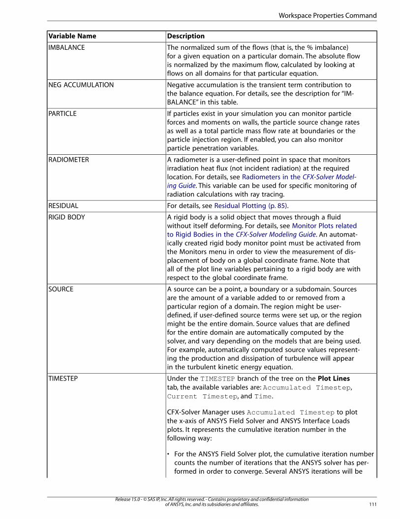
DescriptionVariable Name
The normalized sum of the flows (that is, the % imbalance)for a given equation on a particular domain. The absolute flow
IMBALANCE
is normalized by the maximum flow, calculated by looking atflows on all domains for that particular equation.
Negative accumulation is the transient term contribution tothe balance equation. For details, see the description for “IM-BALANCE” in this table.
NEG ACCUMULATION
If particles exist in your simulation you can monitor particleforces and moments on walls, the particle source change rates
PARTICLE
as well as a total particle mass flow rate at boundaries or theparticle injection region. If enabled, you can also monitorparticle penetration variables.
A radiometer is a user-defined point in space that monitorsirradiation heat flux (not incident radiation) at the required
RADIOMETER
location. For details, see Radiometers in the CFX-Solver Model-
ing Guide. This variable can be used for specific monitoring ofradiation calculations with ray tracing.
For details, see Residual Plotting (p. 85).RESIDUAL
A rigid body is a solid object that moves through a fluidwithout itself deforming. For details, see Monitor Plots related
RIGID BODY
to Rigid Bodies in the CFX-Solver Modeling Guide. An automat-ically created rigid body monitor point must be activated fromthe Monitors menu in order to view the measurement of dis-placement of body on a global coordinate frame. Note thatall of the plot line variables pertaining to a rigid body are withrespect to the global coordinate frame.
A source can be a point, a boundary or a subdomain. Sourcesare the amount of a variable added to or removed from a
SOURCE
particular region of a domain. The region might be user-defined, if user-defined source terms were set up, or the regionmight be the entire domain. Source values that are definedfor the entire domain are automatically computed by thesolver, and vary depending on the models that are being used.For example, automatically computed source values represent-ing the production and dissipation of turbulence will appearin the turbulent kinetic energy equation.
Under the TIMESTEP branch of the tree on the Plot Lines
tab, the available variables are: Accumulated Timestep ,Current Timestep , and Time .
TIMESTEP
CFX-Solver Manager uses Accumulated Timestep to plotthe x-axis of ANSYS Field Solver and ANSYS Interface Loadsplots. It represents the cumulative iteration number in thefollowing way:
• For the ANSYS Field Solver plot, the cumulative iteration numbercounts the number of iterations that the ANSYS solver has per-formed in order to converge. Several ANSYS iterations will be
111Release 15.0 - © SAS IP, Inc. All rights reserved. - Contains proprietary and confidential information
of ANSYS, Inc. and its subsidiaries and affiliates.
Workspace Properties Command
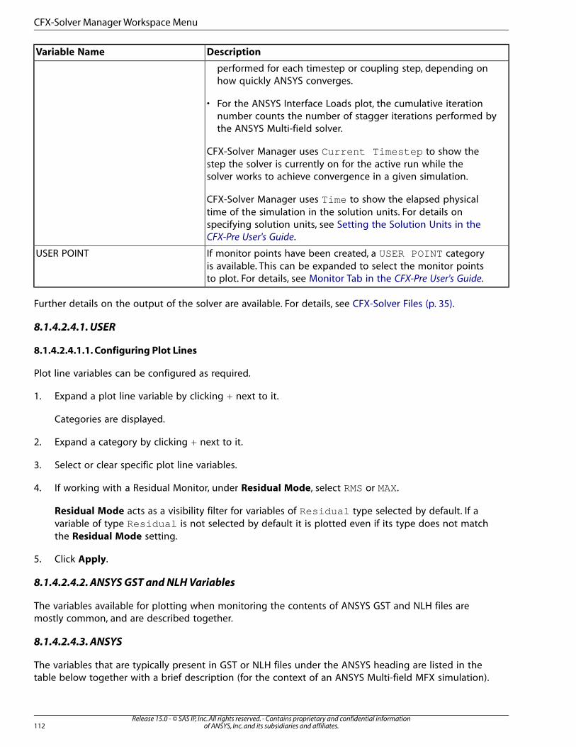
DescriptionVariable Name
performed for each timestep or coupling step, depending onhow quickly ANSYS converges.
• For the ANSYS Interface Loads plot, the cumulative iterationnumber counts the number of stagger iterations performed bythe ANSYS Multi-field solver.
CFX-Solver Manager uses Current Timestep to show thestep the solver is currently on for the active run while thesolver works to achieve convergence in a given simulation.
CFX-Solver Manager uses Time to show the elapsed physicaltime of the simulation in the solution units. For details onspecifying solution units, see Setting the Solution Units in theCFX-Pre User's Guide.
If monitor points have been created, a USER POINT categoryis available. This can be expanded to select the monitor pointsto plot. For details, see Monitor Tab in the CFX-Pre User's Guide.
USER POINT
Further details on the output of the solver are available. For details, see CFX-Solver Files (p. 35).
8.1.4.2.4.1. USER
8.1.4.2.4.1.1. Configuring Plot Lines
Plot line variables can be configured as required.
1. Expand a plot line variable by clicking + next to it.
Categories are displayed.
2. Expand a category by clicking + next to it.
3. Select or clear specific plot line variables.
4. If working with a Residual Monitor, under Residual Mode, select RMS or MAX.
Residual Mode acts as a visibility filter for variables of Residual type selected by default. If avariable of type Residual is not selected by default it is plotted even if its type does not matchthe Residual Mode setting.
5. Click Apply.
8.1.4.2.4.2. ANSYS GST and NLH Variables
The variables available for plotting when monitoring the contents of ANSYS GST and NLH files aremostly common, and are described together.
8.1.4.2.4.3. ANSYS
The variables that are typically present in GST or NLH files under the ANSYS heading are listed in thetable below together with a brief description (for the context of an ANSYS Multi-field MFX simulation).
Release 15.0 - © SAS IP, Inc. All rights reserved. - Contains proprietary and confidential informationof ANSYS, Inc. and its subsidiaries and affiliates.112
CFX-Solver Manager Workspace Menu
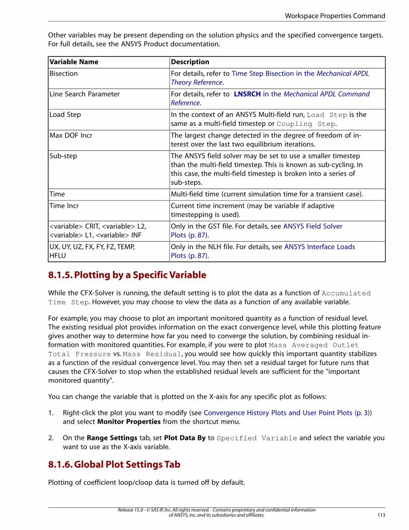
Other variables may be present depending on the solution physics and the specified convergence targets.For full details, see the ANSYS Product documentation.
DescriptionVariable Name
For details, refer to Time Step Bisection in the Mechanical APDL
Theory Reference.Bisection
For details, refer to LNSRCH in the Mechanical APDL Command
Reference.Line Search Parameter
In the context of an ANSYS Multi-field run, Load Step is thesame as a multi-field timestep or Coupling Step .
Load Step
The largest change detected in the degree of freedom of in-terest over the last two equilibrium iterations.
Max DOF Incr
The ANSYS field solver may be set to use a smaller timestepthan the multi-field timestep. This is known as sub-cycling. In
Sub-step
this case, the multi-field timestep is broken into a series ofsub-steps.
Multi-field time (current simulation time for a transient case).Time
Current time increment (may be variable if adaptivetimestepping is used).
Time Incr
Only in the GST file. For details, see ANSYS Field SolverPlots (p. 87).
<variable> CRIT, <variable> L2,<variable> L1, <variable> INF
Only in the NLH file. For details, see ANSYS Interface LoadsPlots (p. 87).
UX, UY, UZ, FX, FY, FZ, TEMP,HFLU
8.1.5. Plotting by a Specific Variable
While the CFX-Solver is running, the default setting is to plot the data as a function of AccumulatedTime Step . However, you may choose to view the data as a function of any available variable.
For example, you may choose to plot an important monitored quantity as a function of residual level.The existing residual plot provides information on the exact convergence level, while this plotting featuregives another way to determine how far you need to converge the solution, by combining residual in-formation with monitored quantities. For example, if you were to plot Mass Averaged OutletTotal Pressure vs. Mass Residual , you would see how quickly this important quantity stabilizesas a function of the residual convergence level. You may then set a residual target for future runs thatcauses the CFX-Solver to stop when the established residual levels are sufficient for the "importantmonitored quantity".
You can change the variable that is plotted on the X-axis for any specific plot as follows:
1. Right-click the plot you want to modify (see Convergence History Plots and User Point Plots (p. 3))and select Monitor Properties from the shortcut menu.
2. On the Range Settings tab, set Plot Data By to Specified Variable and select the variable youwant to use as the X-axis variable.
8.1.6. Global Plot Settings Tab
Plotting of coefficient loop/cloop data is turned off by default.
113Release 15.0 - © SAS IP, Inc. All rights reserved. - Contains proprietary and confidential information
of ANSYS, Inc. and its subsidiaries and affiliates.
Workspace Properties Command

For transient runs, this selects or clears plotting of cloop data for each inner loop. This is in addition toplotting data for each outer loop/timestep. For details, see Transient Residual Plotting (p. 86).
Note
As turning on the cloop setting results in a three to seven times increase in the size of themonitor data file, it affects the performance of the CFX-Solver Manager.
1. Select Workspace > Workspace Properties > Global Plot Settings.
2. Select or clear Plot Coefficient Loop Data.
3. Under Plot Data By select Time Step or Simulation Time .
Variables are plotted against accumulated Time Step (the default) or against SimulationTime . The latter is useful when using non-uniform timesteps.
8.2. New Monitor Command
You can use this command to create a new monitor. However, if other properties associated with aworkspace need to be defined, use the Workspace Properties dialog box instead. Monitors can thenbe created as required.
• Workspace Properties Command (p. 105)
• Monitors Tab (p. 106)
8.3. Stop Current Run Command
To stop the CFX-Solver as soon as possible, use one of the following methods:
• Select Workspace > Stop Current Run.
• Click Stop Current Run .
If running CFX-Solver from the command line, use the command: cfx5stop . For an example of thecfx5stop command, see Command-Line Samples (p. 141).
When CFX-Solver stops, the run is marked as finished, and a message appears. This message names therun and specifies it has terminated at your request. Additional information about the run is also listed.Once manually terminated, a run can be manipulated in the same way that a completed run can.
8.3.1. Stopping Runs Using Mesh Adaption
If a stop current run command is issued for a run that uses mesh adaption, then only the current CFX-Solver run is terminated; the overall simulation, which includes equation solution and mesh adaption,is not. The CFX-Solver is automatically restarted after executing the next adaption step (if any remain),and the simulation continues.
8.3.2. Stopping Runs Using Remeshing
If a stop current run command is issued for a run that uses remeshing, then the overall simulation isterminated.
Release 15.0 - © SAS IP, Inc. All rights reserved. - Contains proprietary and confidential informationof ANSYS, Inc. and its subsidiaries and affiliates.114
CFX-Solver Manager Workspace Menu
8.3.3. Stopping Runs Using External Solver Couplings
If a stop current run command is issued for a run that uses external solver couplings (for example, ANSYSMulti-field), then the overall simulation is. For ANSYS Multi-field couplings, termination occurs at theend of the current Load Step, for details see the Mechanical APDL Coupled-Field Analysis Guide in theMechanical APDL Coupled-Field Analysis Guide. In particular, steady state analyses will run until completion,and transient analyses will run until the end of the current timestep.
8.3.4. Stopping Multi-Configuration Runs
If a stop run command is issued in a workspace for a specific configuration, then only the current CFX-Solver run for that configuration will be terminated; the overall simulation is not. All remaining config-urations that are defined for the simulation are subsequently run (unless a stop run command is alsoissued for them). If a stop run command is issued in the simulation-level workspace, which is labeledaccording to the name of the multi-configuration CFX-Solver Input file (*.mdef ), then the overall sim-ulation is terminated. The CFX-Solver run for the configuration currently being executed is terminatedas soon as possible, and no additional configurations are executed.
8.4. Restart Current Run Command
You can restart a run that is finished or stopped. Restarting a run starts the run with the same settingsas the previous run, including Parallel settings.
There are numerous ways a run can be set up to restart; these are described in Restarting a Run (p. 22).To perform the restart, either:
• Select Workspace > Restart Current Run.
• Click Restart Current Run .
8.5. Backup Run Command
Backing up a run creates a backup file of the results at the end of the timestep that is currently calcu-lating. This file contains sufficient information for restarting a run for visualization. If a solution may bediverging and an intermediate solution must be retained, you should generate backup files.
To back up a run, either:
• Select Workspace > Backup Run.
• Click Backup Run .
The backup file is stored in a subdirectory within the working directory. This subdirectory is given thesame name as the current run.
8.6. Arrange Workspace Command
Arranging the workspace deletes all monitors that are currently showing, regenerates them, and redisplaysthem by optimizing the display based on available screen space. This has no impact on the display ifthe layout type has been toggled to display multiple overlapping tabs. For details, see Toggle LayoutType Command (p. 116).
115Release 15.0 - © SAS IP, Inc. All rights reserved. - Contains proprietary and confidential information
of ANSYS, Inc. and its subsidiaries and affiliates.
Arrange Workspace Command
To arrange the workspace, either:
• Select Workspace > Arrange.
• Click Arrange Workspace .
8.7. Toggle Layout Type Command
Two layout modes exist. One is set up with multiple overlapping tabs used to switch between monitorsand the other displays each monitor in its own window. These may be toggled as required.
To toggle the workspace layout, either:
• Select Workspace > Toggle Layout Types.
• Click Toggle Layout Types .
8.8. Load Layout Command
Layouts can be loaded as required. Before loading a layout, there must be layouts that have been saved.For details, see Save Layout Command (p. 116).
To load a previously saved layout:
1. Select Workspace > Load Layout or click Load Layout .
The Layout File dialog box is displayed.
2. Select the location containing the file to load.
3. Select the file to load.
4. Click Open.
As the new workspace replaces the existing one CFX-Solver Manager requires confirmation thatthe new workspace should overwrite the existing one.
5. Click Yes.
The new layout is loaded.
8.9. Save Layout Command
Once a layout has been configured to display preferred settings views, it can be saved. Once saved,layouts can be loaded as required. For details, see Load Layout Command (p. 116).
This is useful when carrying out different runs for the same problem. For example, there may be a layoutwith preferred settings after changing a boundary condition value. Another layout may be preferredfor viewing a turbulence model. By saving and loading a layout, it is simple to switch between theseviews.
The saved layout fully restores settings only for problems with the same domain and boundary namesas the problem that was selected in the when the layout was saved. If the saved layout is loaded when
Release 15.0 - © SAS IP, Inc. All rights reserved. - Contains proprietary and confidential informationof ANSYS, Inc. and its subsidiaries and affiliates.116
CFX-Solver Manager Workspace Menu
the current problem has different domain and/or boundary names, variables to plot must be reselected.For details, see Defining a Default Plot Monitor (p. 117).
1. Configure the current layout to the appearance to save.
That is, display various monitors, position them, set up the layout type and so on.
2. Select Workspace > Save Layout.
The Layout File dialog box is displayed.
3. If required, set the path location to a different directory.
4. Under File name, type the name of the file to save.
5. Click Save.
If the name already exists, a warning dialog box is displayed.
• Overwrite replaces the old file with the new document.
• Re-select returns to the Layout File dialog box.
• Cancel closes the open dialog boxes.
8.9.1. Defining a Default Plot Monitor
Rather than creating plot monitors manually, one of the existing ones, Turbulent.mst or workspace-basic.mst , can be duplicated and modified.
You can then select your modified file from Workspace > Load Layout in CFX-Solver Manager.
For example, you could modify a copy of the provided monitor file, Turbulent.mst , to include thenew variables as follows:
Change these lines in Turbulent.mst
Variable Rule = CATEGORY = RESIDUAL ; SUBCATEGORY = RMS ; \ EQN_TYPE = list:U-Mom/V-Mom/W-Mom/P-Mass
to
Variable Rule = CATEGORY = RESIDUAL ; SUBCATEGORY = RMS ; \ EQN_TYPE = list:U-Mom/V-Mom/W-Mom/P-Mass/K-TurbKE/E-Diss.K
Note
The monitor file Turbulent.mst can be found in the <CFXROOT>/etc/ directory.
The string for which a search is made can be found from the variable lists in the Plot Lines tab of theMonitors dialog box. For details, see Plot Lines Tab (p. 109).
8.10. View RMS Residuals Command
To display the RMS values of the residuals, select Workspace > View RMS Residuals.
117Release 15.0 - © SAS IP, Inc. All rights reserved. - Contains proprietary and confidential information
of ANSYS, Inc. and its subsidiaries and affiliates.
View RMS Residuals Command
For more information about residuals, see Residual Plotting (p. 85).
8.11. View MAX Residuals Command
To display the MAX values of the residuals, select Workspace > View Max Residuals.
For more information about residuals, see Residual Plotting (p. 85).
8.12. Reset to Default Workspace Command
Resets the default workspace to the state it was in immediately after the run was started, or after afinished run was loaded. This can be useful when retrieving plots that have been accidentally deleted,or when reloading the original plots after a change to their definition.
Note
Resetting the default workspace deletes any custom monitors.
1. Select Workspace > Reset to Default Workspace.
2. Click Yes.
8.13. Close Workspace Command
Closes all windows related to the current run. Any other runs that were open are not affected, and thelast open run prior to the current run is displayed. If the Solver was in progress on the current run, itcontinues to operate in the background. The run can be re-monitored; see Monitor Run in ProgressCommand (p. 99) or Monitor Finished Run Command (p. 99), as appropriate.
Release 15.0 - © SAS IP, Inc. All rights reserved. - Contains proprietary and confidential informationof ANSYS, Inc. and its subsidiaries and affiliates.118
CFX-Solver Manager Workspace Menu

Chapter 9: CFX-Solver Manager Tools Menu
The Tools menu controls layout, plots and text windows that are visible in the viewer. The current runcan also be backed up, restarted or stopped.
Properties for the current workspace can be changed, and new monitors created for simulations.
This chapter describes:9.1. Edit CFX-Solver File Command9.2. Export Command9.3. Export to ANSYS MultiField Command9.4. Interpolate Command9.5. Edit Run In Progress Command9.6. CCL Propagation in Multi-Configuration Simulations9.7. Edit Current Results File Command9.8. Post-Process Results Command9.9.View Environment Command
9.1. Edit CFX-Solver File Command
The command file section of a CFX-Solver input file can be modified. This enables modifications to aCFX-Solver input file without the need to use CFX-Pre. The most useful application of this is in themodification of a simulation when re-running the simulation may be too time consuming.
When a CFX-Solver input file is selected for modification, the Command File Editor is launched. Fordetails, see Editing CFX-Solver Input Files (p. 89).
1. Select Tools > Edit CFX-Solver File.
2. Browse to the directory containing the CFX-Solver input file to edit.
3. Select the CFX-Solver input file.
4. Click Open.
The Command File Editor is launched.
9.2. Export Command
If using tools other than CFD-Post for post-processing, data must be exported to a results file in a sup-ported format. The CFX Export utility can also be run from the command line.
• File Export Utility (p. 155)
• Running cfx5export from the Command Line (p. 172)
There must be a results file to reference before exporting.
119Release 15.0 - © SAS IP, Inc. All rights reserved. - Contains proprietary and confidential information
of ANSYS, Inc. and its subsidiaries and affiliates.
1. Select Tools > Export Results.
The Export dialog box is displayed.
2. Under Source > Results File, click Browse and select a results file for export.
3. Under Source > Domain Selection > Name, select the domain to export.
Where multiple domains exist, select either one domain or all domains to export.
4. Set Timestep, Output Only, Mesh Options and Results Options as required. For details, see GenericExport Options (p. 157).
5. Under Destination > Output Format select CGNS, MSC.Patran , FIELDVIEW, EnSight or CustomUser Export .
• CGNS (p. 158)
• MSC.Patran (p. 161)
• FIELDVIEW (p. 164)
• EnSight (p. 168)
• Custom User Export (p. 170)
6. If required, under Destination > Export File, click Browse and set the output path and filename.
7. Under Destination > <output_format> Options, configure options as required.
The options are dependent on the Output Format. For details, see Output Format (p. 157).
8. Click Export.
Once completed, a message is displayed. Click OK to close it.
9.3. Export to ANSYS MultiField Command
This option is used to produce files for use in Fluid Structure Interaction cases. For details, see Exportto ANSYS Multi-field Solver Dialog Box (p. 155).
1. Select Tools > Export to ANSYS MultiField.
The Export to ANSYS MultiField Solver dialog box is displayed.
2. Under Results File, click Browse and select a results file for export.
3. If required, under Export File, click Browse and modify the default output path and name.
4. Under Domain Name, select the domain to export.
Where multiple domains exist, select either one domain or all domains to export.
Release 15.0 - © SAS IP, Inc. All rights reserved. - Contains proprietary and confidential informationof ANSYS, Inc. and its subsidiaries and affiliates.120
CFX-Solver Manager Tools Menu
5. If required, under Boundary, select the boundaries to export.
6. Under Export Options, configure options as required.
The options are dependent on the export type. For details, see Export to ANSYS Multi-field SolverDialog Box (p. 155).
7. Click Export.
Once completed a message is displayed. Click OK to close it.
9.4. Interpolate Command
ANSYS CFX enables the values from one results file to be interpolated onto a CFX-Solver input filecontaining another mesh.
The major benefit of interpolation is the ability to use the solution from a simple model to provide initialconditions for another, perhaps more complex, model (thereby increasing the likelihood of convergingthe complex model simulation) or to continue a run with a different mesh or other settings.
Interpolation can be used with modified geometry or boundary conditions. Interpolation can also beused to interpolate the solutions from a model with different mesh topology. For example, the initialguess for a problem having one domain can be interpolated from one or more results files having asolution that spans multiple domains. When the shape of the model has changed and the initial valuesfiles do not fully overlap with the new mesh, the CFX-Interpolator extrapolates values for the points inthe new mesh that lie outside the Initial Values File(s), based on the interpolated values on the mappednodes. See Using the CFX-Interpolator in the CFX-Solver Modeling Guide for more details on how theCFX-Interpolator works.
The CFX-Interpolator is most commonly invoked through settings on the Run Definition tab on theConfiguration or Execution Control details view in CFX-Pre, or, the Define Run dialog box of the CFX-Solver Manager. For details, see Run Definition Tab in the CFX-Pre User's Guide, Run Definition Tab inthe CFX-Pre User's Guide and Run Definition Tab (p. 10), respectively.
However, if you want to manually use the interpolator to write variables into a specific Solver Input File(not invoked from the Run Definition tab) then you can choose Tools > Interpolate Results from theCFX-Solver Manager. In this case the specified Mesh File is used as the target file, and will be modifiedby the interpolation process. The text output is written into the CFX-Solver Manager's Interpolationdialog box. You can then run the resulting target file in the CFX-Solver, using the variables written intothe target file by the CFX-Interpolator as the initial conditions for the run.
To manually interpolate the results from a source file to a target file, you can use the Interpolate Results
command as follows:
1. Select Tools > Interpolate Results.
The Interpolation dialog box is displayed.
2. Select the Interpolate method.
3. Set Results File to the name of the source file. You can click Browse to select the file using a browser.
4. Set Mesh File to the name of the target file. You can click Browse to select the target file using a
browser.
121Release 15.0 - © SAS IP, Inc. All rights reserved. - Contains proprietary and confidential information
of ANSYS, Inc. and its subsidiaries and affiliates.
Interpolate Command
You can interpolate onto a CFX-Solver Input file.
5. Optionally, set the precision: under Executable Settings, select Override Default Precision and chooseeither Single or Double.
For details, see Double-Precision Executables (p. 147).
6. If required, under Interpolator Memory, adjust the memory configuration. For details, see ConfiguringMemory for the CFX-Solver (p. 17).
7. Click Interpolate.
The output window on the right displays details of the interpolation process.
Once completed, a message is displayed. Click OK to close it.
You can also run the interpolator from the command line. For details see Using the Command Line toInterpolate Results (p. 123).
Note
• To save the results to a text file, right-click in the text output window and select Save As.
• Interpolating results from a source file to a target file that already contains solution data is notrecommended. See Interpolating Onto a Solver Input File with Results Fields in the CFX-Solver
Modeling Guide for details.
• Following the steps above, the interpolation is performed in Initial Guess mode. See Using theCFX-Interpolator in the CFX-Solver Modeling Guide for details.
To generate a comparison of two files, you can use the Interpolate Results command. The comparisonis stored as new variables with the prefix Difference . These variables can be used in CFD-Post todetermine regions where the solution has changed significantly. A comparison of two files can begenerated as follows:
1. Select Tools > Interpolate Results.
The Interpolation dialog box is displayed.
2. Select the Calculate Differences method.
3. Set Original Results to the name of the original results file. You can click Browse to select the file
using a browser.
4. Set Modified Results to the name of the modified results file. You can click Browse to select the
file using a browser.
5. Optionally, set the precision: under Executable Settings, select Override Default Precision and chooseeither Single or Double.
For details, see Double-Precision Executables (p. 147).
Release 15.0 - © SAS IP, Inc. All rights reserved. - Contains proprietary and confidential informationof ANSYS, Inc. and its subsidiaries and affiliates.122
CFX-Solver Manager Tools Menu
6. If required, under Interpolator Memory, adjust the memory configuration. For details, see ConfiguringMemory for the CFX-Solver (p. 17).
7. Click Calculate Differences.
The output window on the right displays details of the differencing process.
Once completed, a message is displayed. Click OK to close it.
Note
CFD-Post now also supports comparison of two results files without the use of the CFX-Inter-polator. For details, see Case Comparison in the CFD-Post User's Guide.
9.4.1. Using the Command Line to Interpolate Results
In some instances, the cfx5interp script can be used from the command line to initiate an interpol-ation. This section presents a brief introduction to this script. For more information about this script,type <CFXROOT>/cfx5interp -help at the command prompt.
To use the cfx5interp script, enter a command line of the form:
cfx5interp -res <results file> -mesh <CFX-Solver input file> [<arguments>]
where:
• <results file> is the name of a results file that contains a solution.
• <CFX-Solver input file> is the name of a CFX-Solver input file that contains a mesh onto whichthe solution should be interpolated.
• [<arguments>] is an optional list of additional arguments.
cfx5interp rewrites the CFX-Solver input file with the interpolated form of the solution that wasread from the results file. A command of this form would produce the same results as running invokinginterpolation using Tools > Interpolate Results within the CFX-Solver Manager.
You can use the -difference argument to cause the interpolator to produce difference datasets fordifferences in results between two results files. The form of such a statement is:
cfx5interp -difference -from <res file 1> -dest <res file 2> [<arguments>]
where:
• <res file 1> is the name of a results file that contains the original (older) set of fields
• <res file 2> is the name of a results file that contains the newer set of fields
• [<arguments>] is an optional list of additional arguments
cfx5interp calculates the differences between an original set of fields and the newer set, and rewrites<res file 2> with the differencing information included.
123Release 15.0 - © SAS IP, Inc. All rights reserved. - Contains proprietary and confidential information
of ANSYS, Inc. and its subsidiaries and affiliates.
Interpolate Command
The cfx5interp script can run two versions of the interpolator. The newer version (a solver-basedinterpolator) runs by default, and the older one (that was released with ANSYS CFX 10.0) can be invokedby using the -interp-old argument.
When the older interpolator is used, the cfx5interp script is capable of producing a text file of resultsfor specific locations within the fluid domain. This is particularly useful if there is experimental data tovalidate.
To produce a results text file, first create a text file containing the particular vertex coordinates of interest,in the following format:
x(1) y(1) z(1)x(2) y(2) z(2). . . .x(n) y(n) z(n)
Once the vertex file is created, run the old interpolator using a command line of the form:
cfx5interp -vtx <vertex file> -res <results file> -interpolate-old
The old interpolator creates a file with a name of the form: <vertex file>.inn , where nn is chosento make a unique file name. This is a text file that contains the coordinates that are specified in thevertex file, plus the results from the results file interpolated to the vertex locations.
If, in the vertex file, there are coordinates that lie outside of the solution grid, values of 0.0E0 will beassigned for all variables at those coordinates. In other words, results are not extrapolated to a vertexfile.
Note
Some of the values obtained using the cfx5interp script may differ slightly from the valuesobtained using Data Export in CFD-Post. These minor discrepancies result from differentmethods of calculation. Discrepancies are more likely to occur at points that lie very closeto the edge of the mesh elements or in regions of prism and hexahedral elements. Inconsist-encies are likely to be more significant where gradients are large, particularly in the boundarylayer.
9.5. Edit Run In Progress Command
You can edit the CCL definition of a CFX-Solver input file while the solver is running. The changes youmake take effect when saved and the modified CCL is pre-processed for the flow solver. The modifiedCCL may take several iterations to be updated depending on system load, hardware and problem size.
These changes apply only to the run in progress, and do not affect the CFX-Solver input file that wasused to begin the run (if one was used). Before the next outer-loop iteration begins, a backup file named<iteration number>.bak is written to the working directory. The backup file can be used to restartthe run from the point at which the CCL definition was changed, if needed.
Only selected CCL parameters can be dynamically changed. A list of these parameters is in the RULESfile. For details, see RULES File (p. 97).
The Command File Editor can also be used to make changes to the CCL contained in a CFX-Solver inputfile. Changes, when saved, affect the edited CFX-Solver input file only, not any run in progress. For details,see Editing CFX-Solver Input Files (p. 89).
Release 15.0 - © SAS IP, Inc. All rights reserved. - Contains proprietary and confidential informationof ANSYS, Inc. and its subsidiaries and affiliates.124
CFX-Solver Manager Tools Menu
To access the command file editor, select Tools > Edit Run In Progress or click .
Note
The Edit Run in Progress command is not selected for simulations involving ANSYS Multi-field couplings or transient blade row modeling. This constraint exists for simulations involvingANSYS Multi-field couplings because of difficulties involved with updating the MFX settingsin the ANSYS solver during the run.
9.6. CCL Propagation in Multi-Configuration Simulations
The Edit Run in Progress command is selected for the configuration being run, rather than in theglobal (or simulation) level workspace. In addition to applying CCL changes to the running configuration,some or all of the changes are also automatically propagated to subsequent configuration runs. Inparticular:
• Changes made to the LIBRARY section of the CCL (such as material properties, expressions, reactions,etc…) are propagated to all subsequent configurations, and
• Changes made to the FLOW section of the CCL (such as analysis type, boundary conditions, solver andoutput controls, etc…) are propagated to all subsequent runs of the current configuration.
9.7. Edit Current Results File Command
Edit the CFX-Solver Results file in the current workspace (if available). This feature is available only whenthere is a finished CFX-Solver Results file in the current workspace. For details, see Editing CFX-SolverInput Files (p. 89).
To access the command file editor, select Tools > Edit Current Results File or click . The Command
File Editor is launched and the current results file is opened.
9.8. Post-Process Results Command
Loads the CFD-Post post-processor. For details, see Overview of CFD-Post in the CFD-Post User's Guide.
1. Select Tools > Post-Process Results.
The Start CFD-Post dialog box is displayed.
2. Under Results File, click Browse and select a results file to load into CFD-Post.
3. If you want to load two results files into CFD-Post together, check Specify Additional Results File, andselect another results file to load.
4. Select Multi-Configuration Load Options in order to control how the results of a multi-configurationrun are loaded, or to load just the last case of such a run.
5. Select or clear Shut down CFX-Solver Manager.
If selected, ANSYS CFX-Solver Manager is shut down before CFD-Post is launched.
6. Click OK.
125Release 15.0 - © SAS IP, Inc. All rights reserved. - Contains proprietary and confidential information
of ANSYS, Inc. and its subsidiaries and affiliates.
Post-Process Results Command

9.9. View Environment Command
Used to display a complete list of environment variables associated with the CFX-Solver Manager andtheir settings.
1. Select Tools > View Environment.
The Solver Manager Environment dialog box is displayed.
2. Click Save to export the content to a text file.
Release 15.0 - © SAS IP, Inc. All rights reserved. - Contains proprietary and confidential informationof ANSYS, Inc. and its subsidiaries and affiliates.126
CFX-Solver Manager Tools Menu
Chapter 10: CFX-Solver Manager Monitors Menu
The Monitors menu sets the display options for plots of your simulation.
Each menu option has a submenu. This is used to specify display options for a given category. Selectedoptions will display the related plot.
Residuals are combined by default in the CFX-Solver Manager. Residuals for each domain can be displayedas required by selecting the residuals by domain in the submenu for each residual type.
127Release 15.0 - © SAS IP, Inc. All rights reserved. - Contains proprietary and confidential information
of ANSYS, Inc. and its subsidiaries and affiliates.

Release 15.0 - © SAS IP, Inc. All rights reserved. - Contains proprietary and confidential informationof ANSYS, Inc. and its subsidiaries and affiliates.128

Chapter 11: Starting the CFX-Solver from the Command Line
The CFX-Solver is a separate module of CFX that has no graphical user interface. You can start CFX-Solver from the command line by executing the following command:
cfx5solve [ options]
where [options] denotes the options applicable during a command-line run.
This chapter discusses how to run CFX-Solver in a batch mode and describes the supported command-line options in the following sections:
11.1. Command-Line Use11.2. Command-Line Options and Keywords for cfx5solve11.3. Command-Line Samples
Note
You can also use CFX-Solver Manager to start CFX-Solver. The graphical user interface of theCFX-Solver Manager enables you to set various options, allows easier control of the solutionprocess, and provides some visual details as the solution emerges. For details, see CFX-SolverManager Basics (p. 1).
11.1. Command-Line Use
CFX-Solver Manager and CFX-Solver can be launched from a command line as follows:
• The basic command to start CFX-Solver Manager is cfx5solve .
The more general form of the command is:
cfx5solve [-interactive [-definition <file>]][-display <display>] [-help][-solver <executable>] [-verbose]
where [ ] denotes a discretionary option, | separates mutually exclusive options, and < > denotes thatsubstitution of a suitable value is required. All other options are keywords, some of which have ashort form.
• The basic command to start the CFX-Solver using the CFX-Solver input file named <file> is:
cfx5solve -def <file> [-help] [-initial <file>][-double | -single][-nosave|-save] [-name <name>] [-size <factor>][-solver <executable>] [-partition <number of partitions>][-parallel] [-parfile <file>] [-serial] [-verbose]
where [ ] denotes a discretionary option, | separates mutually exclusive options, and < > denotes thatsubstitution of a suitable value is required. All other options are keywords, some of which have ashort form.
How you invoke a command line depends on your operating system:
129Release 15.0 - © SAS IP, Inc. All rights reserved. - Contains proprietary and confidential information
of ANSYS, Inc. and its subsidiaries and affiliates.
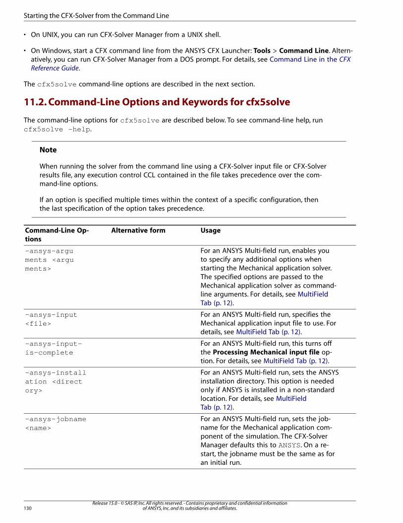
• On UNIX, you can run CFX-Solver Manager from a UNIX shell.
• On Windows, start a CFX command line from the ANSYS CFX Launcher: Tools > Command Line. Altern-atively, you can run CFX-Solver Manager from a DOS prompt. For details, see Command Line in the CFX
Reference Guide.
The cfx5solve command-line options are described in the next section.
11.2. Command-Line Options and Keywords for cfx5solve
The command-line options for cfx5solve are described below. To see command-line help, runcfx5solve -help .
Note
When running the solver from the command line using a CFX-Solver input file or CFX-Solverresults file, any execution control CCL contained in the file takes precedence over the com-mand-line options.
If an option is specified multiple times within the context of a specific configuration, thenthe last specification of the option takes precedence.
UsageAlternative formCommand-Line Op-
tions
For an ANSYS Multi-field run, enables youto specify any additional options when
-ansys-arguments <arguments> starting the Mechanical application solver.
The specified options are passed to theMechanical application solver as command-line arguments. For details, see MultiFieldTab (p. 12).
For an ANSYS Multi-field run, specifies theMechanical application input file to use. Fordetails, see MultiField Tab (p. 12).
-ansys-input<file>
For an ANSYS Multi-field run, this turns offthe Processing Mechanical input file op-tion. For details, see MultiField Tab (p. 12).
-ansys-input-is-complete
For an ANSYS Multi-field run, sets the ANSYSinstallation directory. This option is needed
-ansys-installation <directory> only if ANSYS is installed in a non-standard
location. For details, see MultiFieldTab (p. 12).
For an ANSYS Multi-field run, sets the job-name for the Mechanical application com-
-ansys-jobname<name>
ponent of the simulation. The CFX-SolverManager defaults this to ANSYS. On a re-start, the jobname must be the same as foran initial run.
Release 15.0 - © SAS IP, Inc. All rights reserved. - Contains proprietary and confidential informationof ANSYS, Inc. and its subsidiaries and affiliates.130
Starting the CFX-Solver from the Command Line
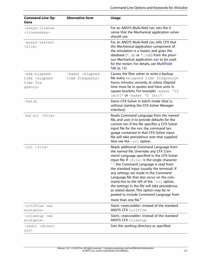
UsageAlternative formCommand-Line Op-
tions
For an ANSYS Multi-field run, sets the li-cense that the Mechanical application solvershould use.
-ansys-license<licensekey>
For an ANSYS Multi-field run, tells CFX thatthe Mechanical application component of
-ansys-restart<file>
the simulation is a restart, and gives thedatabase (*.db or *.rdb ) from the previ-ous Mechanical application run to be usedfor the restart. For details, see MultiFieldTab (p. 12).
Causes the flow solver to write a backupfile every <elapsed time frequency>
-baket <elapsedtime frequency>
-bak-elapsed-time <elapsed
hours, minutes, seconds, et cetera. Elapsedtime frequency> time must be in quotes and have units in
square brackets. For example: -baket “10[min]” or -baket “ 5 [hr] ” .
Starts CFX-Solver in batch mode (that is,without starting the CFX-Solver Managerinterface).
-batch
Reads Command Language from the namedfile, and uses it to provide defaults for the
-bg-ccl <file>
current run. If the file specifies a CFX-Solverinput file for the run, the command lan-guage contained in that CFX-Solver inputfile will take precedence over that supplied.Also see the -ccl option.
Reads additional Command Language fromthe named file. Overrides any CFX Com-
-ccl <file>
mand Language specified in the CFX-Solverinput file. If <file> is the single character'- ', the Command Language is read fromthe standard input (usually the terminal). Ifany settings are made in the CommandLanguage file that also occur on the com-mand line to the left of the -ccl option,the settings in the file will take precedence,as stated above. This option may be re-peated to include Command Language from
more than one file.a
Starts <executable> instead of the standardANSYS CFX ccl2flow .
-ccl2flow <executable>
Starts <executable> instead of the standardANSYS CFX cclsetup .
-cclsetup <executable>
Sets the working directory as specified.-chdir <directory>
131Release 15.0 - © SAS IP, Inc. All rights reserved. - Contains proprietary and confidential information
of ANSYS, Inc. and its subsidiaries and affiliates.
Command-Line Options and Keywords for cfx5solve
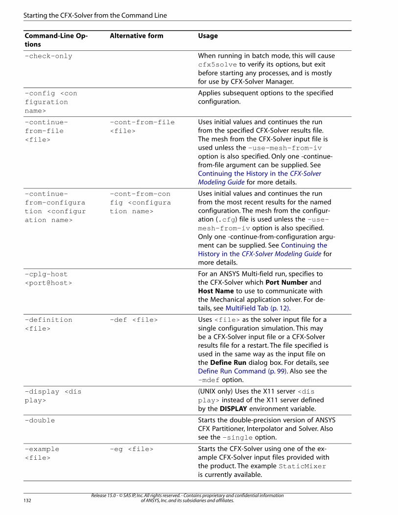
UsageAlternative formCommand-Line Op-
tions
When running in batch mode, this will causecfx5solve to verify its options, but exit
-check-only
before starting any processes, and is mostlyfor use by CFX-Solver Manager.
Applies subsequent options to the specifiedconfiguration.
-config <configurationname>
Uses initial values and continues the runfrom the specified CFX-Solver results file.
-cont-from-file<file>
-continue-from-file<file> The mesh from the CFX-Solver input file is
used unless the -use-mesh-from-ivoption is also specified. Only one -continue-from-file argument can be supplied. SeeContinuing the History in the CFX-Solver
Modeling Guide for more details.
Uses initial values and continues the runfrom the most recent results for the named
-cont-from-config <configuration name>
-continue-from-configuration <configuration name>
configuration. The mesh from the configur-ation (.cfg ) file is used unless the -use-mesh-from-iv option is also specified.Only one -continue-from-configuration argu-ment can be supplied. See Continuing theHistory in the CFX-Solver Modeling Guide formore details.
For an ANSYS Multi-field run, specifies tothe CFX-Solver which Port Number and
-cplg-host<port@host>
Host Name to use to communicate withthe Mechanical application solver. For de-tails, see MultiField Tab (p. 12).
Uses <file> as the solver input file for asingle configuration simulation. This may
-def <file>-definition<file>
be a CFX-Solver input file or a CFX-Solverresults file for a restart. The file specified isused in the same way as the input file onthe Define Run dialog box. For details, seeDefine Run Command (p. 99). Also see the-mdef option.
(UNIX only) Uses the X11 server <display> instead of the X11 server definedby the DISPLAY environment variable.
-display <display>
Starts the double-precision version of ANSYSCFX Partitioner, Interpolator and Solver. Alsosee the -single option.
-double
Starts the CFX-Solver using one of the ex-ample CFX-Solver input files provided with
-eg <file>-example<file>
the product. The example StaticMixeris currently available.
Release 15.0 - © SAS IP, Inc. All rights reserved. - Contains proprietary and confidential informationof ANSYS, Inc. and its subsidiaries and affiliates.132
Starting the CFX-Solver from the Command Line
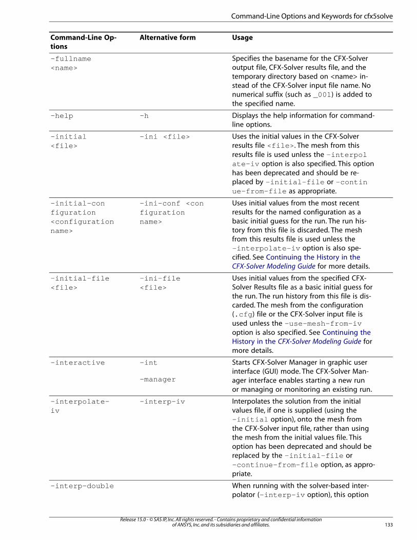
UsageAlternative formCommand-Line Op-
tions
Specifies the basename for the CFX-Solveroutput file, CFX-Solver results file, and the
-fullname<name>
temporary directory based on <name> in-stead of the CFX-Solver input file name. Nonumerical suffix (such as _001 ) is added tothe specified name.
Displays the help information for command-line options.
-h-help
Uses the initial values in the CFX-Solverresults file <file> . The mesh from this
-ini <file>-initial<file>
results file is used unless the -interpolate-iv option is also specified. This optionhas been deprecated and should be re-placed by -initial-file or -continue-from-file as appropriate.
Uses initial values from the most recentresults for the named configuration as a
-ini-conf <configurationname>
-initial-configuration<configurationname>
basic initial guess for the run. The run his-tory from this file is discarded. The meshfrom this results file is used unless the-interpolate-iv option is also spe-cified. See Continuing the History in theCFX-Solver Modeling Guide for more details.
Uses initial values from the specified CFX-Solver Results file as a basic initial guess for
-ini-file<file>
-initial-file<file>
the run. The run history from this file is dis-carded. The mesh from the configuration(.cfg ) file or the CFX-Solver input file isused unless the -use-mesh-from-ivoption is also specified. See Continuing theHistory in the CFX-Solver Modeling Guide formore details.
Starts CFX-Solver Manager in graphic userinterface (GUI) mode. The CFX-Solver Man-
-int
-manager
-interactive
ager interface enables starting a new runor managing or monitoring an existing run.
Interpolates the solution from the initialvalues file, if one is supplied (using the
-interp-iv-interpolate-iv
-initial option), onto the mesh fromthe CFX-Solver input file, rather than usingthe mesh from the initial values file. Thisoption has been deprecated and should bereplaced by the -initial-file or-continue-from-file option, as appro-priate.
When running with the solver-based inter-polator (-interp-iv option), this option
-interp-double
133Release 15.0 - © SAS IP, Inc. All rights reserved. - Contains proprietary and confidential information
of ANSYS, Inc. and its subsidiaries and affiliates.
Command-Line Options and Keywords for cfx5solve

UsageAlternative formCommand-Line Op-
tions
will select the double-precision version ofthe interpolator. It will not override the-interpolator option if both are used.
Uses the single precision ANSYS CFX Inter-polator executable.
-interp-single
When running with the interpolator (-interp-iv option), this option will start
-interpolator<executable>
<executable> instead of the default in-terpolator.
Keeps the .job file after an ANSYS CFXSolver run. This file contains a brief sum-
-job
mary of various solution values, and is mostuseful for regression purposes.
Keeps job file after an ANSYS CFX Partitionerrun. This file contains a brief summary of
-jobp-job-part
various solution values, and is most usefulfor regression purposes.
Sets the maximum elapsed time (wall clocktime) that CFX-Solver will run. Elapsed time
-maxet <elapsedtime>
-max-elapsed-time <elapsedtime> must be in quotes and have correct units
in square brackets. For example: -maxet“ 10 [min] ” or -maxet “ 5 [hr] ” .
Uses <file> as the solver input file. Thismay be a multi-configuration definition file
-mdef <file>-mdefinition<file>
or results file for a restart (that is, .mdef or.mres , respectively). The file specified isused in the same way as the input file onthe Define Run dialog box. For details, seeDefine Run Command (p. 99).
Use this option to specify one of the follow-ing MFX run modes for an ANSYS Multi-fieldrun:
-mfx-run-mode<mode>
"Start ANSYS and CFX"
"Start ANSYS only"
"Start CFX only"
"Process Input File only"
For details, see MultiField Tab (p. 12).
When starting ANSYS CFX-Solver Manager,use this option to monitor the run represen-
-monitor<file>
ted by <file> , which may be a CFX-Solverresults file or CFX-Solver output file.
Release 15.0 - © SAS IP, Inc. All rights reserved. - Contains proprietary and confidential informationof ANSYS, Inc. and its subsidiaries and affiliates.134
Starting the CFX-Solver from the Command Line
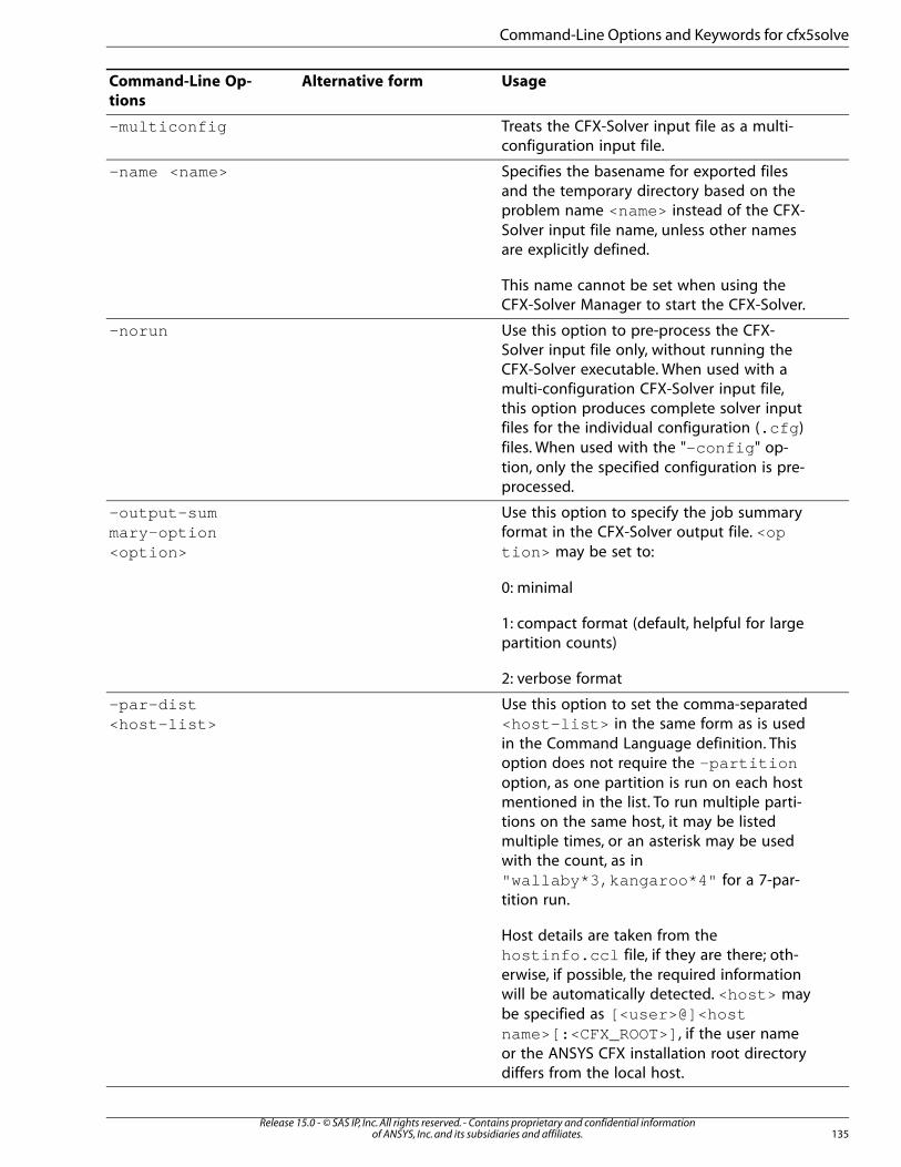
UsageAlternative formCommand-Line Op-
tions
Treats the CFX-Solver input file as a multi-configuration input file.
-multiconfig
Specifies the basename for exported filesand the temporary directory based on the
-name <name>
problem name <name> instead of the CFX-Solver input file name, unless other namesare explicitly defined.
This name cannot be set when using theCFX-Solver Manager to start the CFX-Solver.
Use this option to pre-process the CFX-Solver input file only, without running the
-norun
CFX-Solver executable. When used with amulti-configuration CFX-Solver input file,this option produces complete solver inputfiles for the individual configuration (.cfg )files. When used with the "-config " op-tion, only the specified configuration is pre-processed.
Use this option to specify the job summaryformat in the CFX-Solver output file. <option> may be set to:
-output-summary-option<option>
0: minimal
1: compact format (default, helpful for largepartition counts)
2: verbose format
Use this option to set the comma-separated<host-list> in the same form as is used
-par-dist<host-list>
in the Command Language definition. Thisoption does not require the -partitionoption, as one partition is run on each hostmentioned in the list. To run multiple parti-tions on the same host, it may be listedmultiple times, or an asterisk may be usedwith the count, as in"wallaby*3,kangaroo*4" for a 7-par-tition run.
Host details are taken from thehostinfo.ccl file, if they are there; oth-erwise, if possible, the required informationwill be automatically detected. <host> maybe specified as [<user>@]<hostname>[:<CFX_ROOT>] , if the user nameor the ANSYS CFX installation root directorydiffers from the local host.
135Release 15.0 - © SAS IP, Inc. All rights reserved. - Contains proprietary and confidential information
of ANSYS, Inc. and its subsidiaries and affiliates.
Command-Line Options and Keywords for cfx5solve
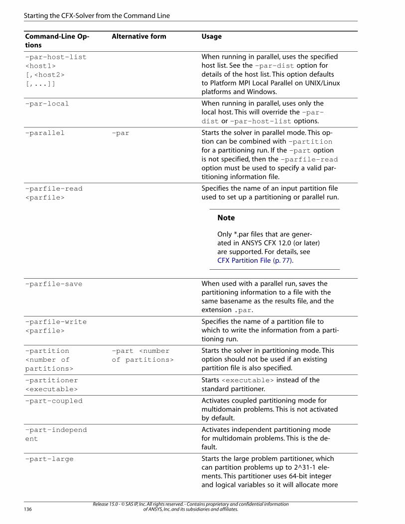
UsageAlternative formCommand-Line Op-
tions
When running in parallel, uses the specifiedhost list. See the -par-dist option for
-par-host-list<host1>
details of the host list. This option defaults[,<host2>[,...]] to Platform MPI Local Parallel on UNIX/Linux
platforms and Windows.
When running in parallel, uses only thelocal host. This will override the -par-dist or -par-host-list options.
-par-local
Starts the solver in parallel mode. This op-tion can be combined with -partition
-par-parallel
for a partitioning run. If the -part optionis not specified, then the -parfile-readoption must be used to specify a valid par-titioning information file.
Specifies the name of an input partition fileused to set up a partitioning or parallel run.
Note
Only *.par files that are gener-ated in ANSYS CFX 12.0 (or later)
-parfile-read<parfile>
are supported. For details, seeCFX Partition File (p. 77).
When used with a parallel run, saves thepartitioning information to a file with the
-parfile-save
same basename as the results file, and theextension .par .
Specifies the name of a partition file towhich to write the information from a parti-tioning run.
-parfile-write<parfile>
Starts the solver in partitioning mode. Thisoption should not be used if an existingpartition file is also specified.
-part <numberof partitions>
-partition<number ofpartitions>
Starts <executable> instead of thestandard partitioner.
-partitioner<executable>
Activates coupled partitioning mode formultidomain problems. This is not activatedby default.
-part-coupled
Activates independent partitioning modefor multidomain problems. This is the de-fault.
-part-independent
Starts the large problem partitioner, whichcan partition problems up to 2^31-1 ele-
-part-large
ments. This partitioner uses 64-bit integerand logical variables so it will allocate more
Release 15.0 - © SAS IP, Inc. All rights reserved. - Contains proprietary and confidential informationof ANSYS, Inc. and its subsidiaries and affiliates.136
Starting the CFX-Solver from the Command Line
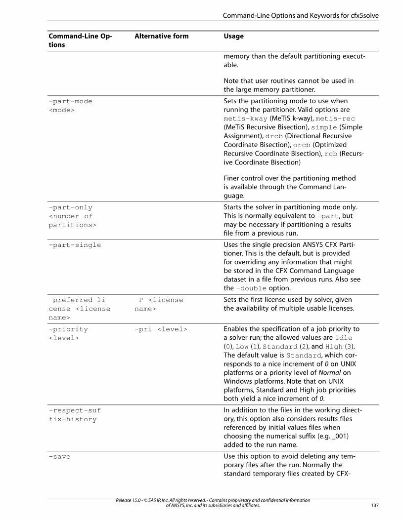
UsageAlternative formCommand-Line Op-
tions
memory than the default partitioning execut-able.
Note that user routines cannot be used inthe large memory partitioner.
Sets the partitioning mode to use whenrunning the partitioner. Valid options are
-part-mode<mode>
metis-kway (MeTiS k-way), metis-rec(MeTiS Recursive Bisection), simple (SimpleAssignment), drcb (Directional RecursiveCoordinate Bisection), orcb (OptimizedRecursive Coordinate Bisection), rcb (Recurs-ive Coordinate Bisection)
Finer control over the partitioning methodis available through the Command Lan-guage.
Starts the solver in partitioning mode only.This is normally equivalent to -part , but
-part-only<number ofpartitions> may be necessary if partitioning a results
file from a previous run.
Uses the single precision ANSYS CFX Parti-tioner. This is the default, but is provided
-part-single
for overriding any information that mightbe stored in the CFX Command Languagedataset in a file from previous runs. Also seethe -double option.
Sets the first license used by solver, giventhe availability of multiple usable licenses.
-P <licensename>
-preferred-license <licensename>
Enables the specification of a job priority toa solver run; the allowed values are Idle
-pri <level>-priority<level>
(0), Low (1), Standard (2), and High (3).The default value is Standard , which cor-responds to a nice increment of 0 on UNIXplatforms or a priority level of Normal onWindows platforms. Note that on UNIXplatforms, Standard and High job prioritiesboth yield a nice increment of 0.
In addition to the files in the working direct-ory, this option also considers results files
-respect-suffix-history
referenced by initial values files whenchoosing the numerical suffix (e.g. _001)added to the run name.
Use this option to avoid deleting any tem-porary files after the run. Normally the
-save
standard temporary files created by CFX-
137Release 15.0 - © SAS IP, Inc. All rights reserved. - Contains proprietary and confidential information
of ANSYS, Inc. and its subsidiaries and affiliates.
Command-Line Options and Keywords for cfx5solve
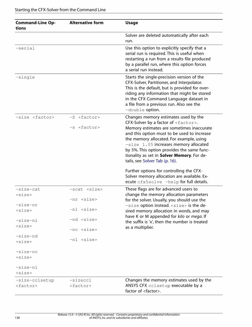
UsageAlternative formCommand-Line Op-
tions
Solver are deleted automatically after eachrun.
Use this option to explicitly specify that aserial run is required. This is useful when
-serial
restarting a run from a results file producedby a parallel run, where this option forcesa serial run instead.
Starts the single-precision version of theCFX-Solver, Partitioner, and Interpolator.
-single
This is the default, but is provided for over-riding any information that might be storedin the CFX Command Language dataset ina file from a previous run. Also see the-double option.
Changes memory estimates used by theCFX-Solver by a factor of <factor> .
-S <factor>
-s <factor>
-size <factor>
Memory estimates are sometimes inaccurateand this option must to be used to increasethe memory allocated. For example, using-size 1.05 increases memory allocatedby 5%. This option provides the same func-tionality as set in Solver Memory. For de-tails, see Solver Tab (p. 16).
Further options for controlling the CFX-Solver memory allocation are available. Ex-ecute cfx5solve -help for full details.
These flags are for advanced users tochange the memory allocation parameters
-scat <size>
-nr <size>
-size-cat<size>
-size-nr<size>
for the solver. Usually, you should use the-size option instead. <size> is the de-sired memory allocation in words, and may-ni <size>
-nd <size>-size-ni<size>
have K or M appended for kilo or mega. Ifthe suffix is 'x', then the number is treatedas a multiplier.-nc <size>
-size-nd<size> -nl <size>
-size-nc<size>
-size-nl<size>
Changes the memory estimates used by theANSYS CFX cclsetup executable by afactor of <factor>.
-sizeccl<factor>
-size-cclsetup<factor>
Release 15.0 - © SAS IP, Inc. All rights reserved. - Contains proprietary and confidential informationof ANSYS, Inc. and its subsidiaries and affiliates.138
Starting the CFX-Solver from the Command Line
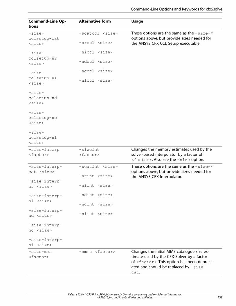
UsageAlternative formCommand-Line Op-
tions
These options are the same as the -size-*options above, but provide sizes needed forthe ANSYS CFX CCL Setup executable.
-scatccl <size>
-nrccl <size>
-niccl <size>
-size-cclsetup-cat<size>
-size-cclsetup-nr<size> -ndccl <size>
-ncccl <size>-size-cclsetup-ni<size>
-nlccl <size>
-size-cclsetup-nd<size>
-size-cclsetup-nc<size>
-size-cclsetup-nl<size>
Changes the memory estimates used by thesolver-based interpolator by a factor of<factor> . Also see the -size option.
-sizeint<factor>
-size-interp<factor>
These options are the same as the -size-*options above, but provide sizes needed forthe ANSYS CFX Interpolator.
-scatint <size>
-nrint <size>
-niint <size>
-size-interp-cat <size>
-size-interp-nr <size>
-ndint <size>-size-interp-ni <size>
-ncint <size>
-size-interp-nd <size> -nlint <size>
-size-interp-nc <size>
-size-interp-nl <size>
Changes the initial MMS catalogue size es-timate used by the CFX-Solver by a factor
-smms <factor>-size-mms<factor>
of <factor> . This option has been deprec-ated and should be replaced by -size-cat .
139Release 15.0 - © SAS IP, Inc. All rights reserved. - Contains proprietary and confidential information
of ANSYS, Inc. and its subsidiaries and affiliates.
Command-Line Options and Keywords for cfx5solve
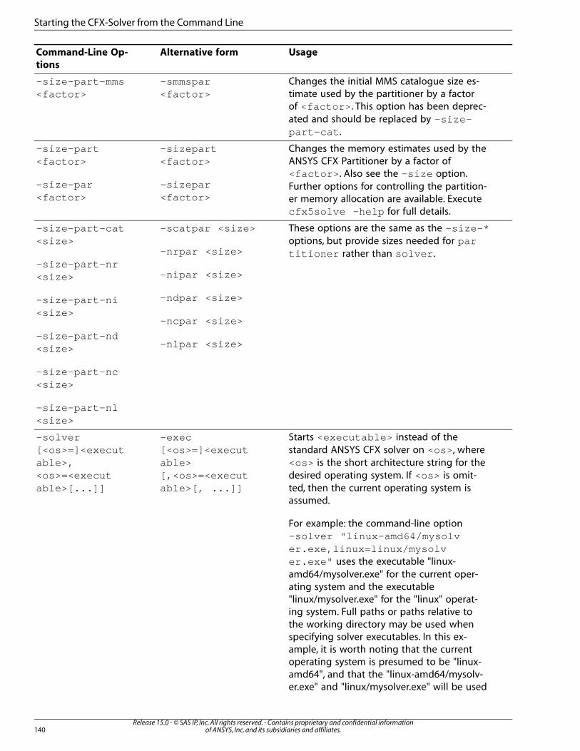
UsageAlternative formCommand-Line Op-
tions
Changes the initial MMS catalogue size es-timate used by the partitioner by a factor
-smmspar<factor>
-size-part-mms<factor>
of <factor> . This option has been deprec-ated and should be replaced by -size-part-cat .
Changes the memory estimates used by theANSYS CFX Partitioner by a factor of
-sizepart<factor>
-size-part<factor>
<factor> . Also see the -size option.-sizepar<factor>
-size-par<factor>
Further options for controlling the partition-er memory allocation are available. Executecfx5solve -help for full details.
These options are the same as the -size-*options, but provide sizes needed for partitioner rather than solver .
-scatpar <size>
-nrpar <size>
-nipar <size>
-size-part-cat<size>
-size-part-nr<size>
-ndpar <size>-size-part-ni<size>
-ncpar <size>
-size-part-nd<size> -nlpar <size>
-size-part-nc<size>
-size-part-nl<size>
Starts <executable> instead of thestandard ANSYS CFX solver on <os> , where
-exec[<os>=]<execut
-solver[<os>=]<execut
<os> is the short architecture string for theable>able>,desired operating system. If <os> is omit-[,<os>=<execut
able>[, ...]]<os>=<executable>[...]] ted, then the current operating system is
assumed.
For example: the command-line option-solver "linux-amd64/mysolver.exe,linux=linux/mysolver.exe" uses the executable "linux-amd64/mysolver.exe" for the current oper-ating system and the executable"linux/mysolver.exe" for the "linux" operat-ing system. Full paths or paths relative tothe working directory may be used whenspecifying solver executables. In this ex-ample, it is worth noting that the currentoperating system is presumed to be "linux-amd64", and that the "linux-amd64/mysolv-er.exe" and "linux/mysolver.exe" will be used
Release 15.0 - © SAS IP, Inc. All rights reserved. - Contains proprietary and confidential informationof ANSYS, Inc. and its subsidiaries and affiliates.140
Starting the CFX-Solver from the Command Line
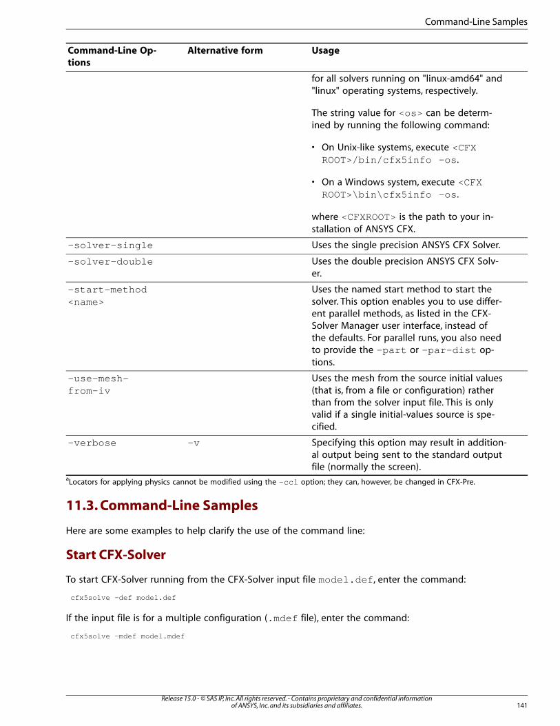
UsageAlternative formCommand-Line Op-
tions
for all solvers running on "linux-amd64" and"linux" operating systems, respectively.
The string value for <os> can be determ-ined by running the following command:
• On Unix-like systems, execute <CFXROOT>/bin/cfx5info -os .
• On a Windows system, execute <CFXROOT>\bin\cfx5info -os .
where <CFXROOT> is the path to your in-stallation of ANSYS CFX.
Uses the single precision ANSYS CFX Solver.-solver-single
Uses the double precision ANSYS CFX Solv-er.
-solver-double
Uses the named start method to start thesolver. This option enables you to use differ-
-start-method<name>
ent parallel methods, as listed in the CFX-Solver Manager user interface, instead ofthe defaults. For parallel runs, you also needto provide the -part or -par-dist op-tions.
Uses the mesh from the source initial values(that is, from a file or configuration) rather
-use-mesh-from-iv
than from the solver input file. This is onlyvalid if a single initial-values source is spe-cified.
Specifying this option may result in addition-al output being sent to the standard outputfile (normally the screen).
-v-verbose
aLocators for applying physics cannot be modified using the -ccl option; they can, however, be changed in CFX-Pre.
11.3. Command-Line Samples
Here are some examples to help clarify the use of the command line:
Start CFX-Solver
To start CFX-Solver running from the CFX-Solver input file model.def , enter the command:
cfx5solve -def model.def
If the input file is for a multiple configuration (.mdef file), enter the command:
cfx5solve -mdef model.mdef
141Release 15.0 - © SAS IP, Inc. All rights reserved. - Contains proprietary and confidential information
of ANSYS, Inc. and its subsidiaries and affiliates.
Command-Line Samples
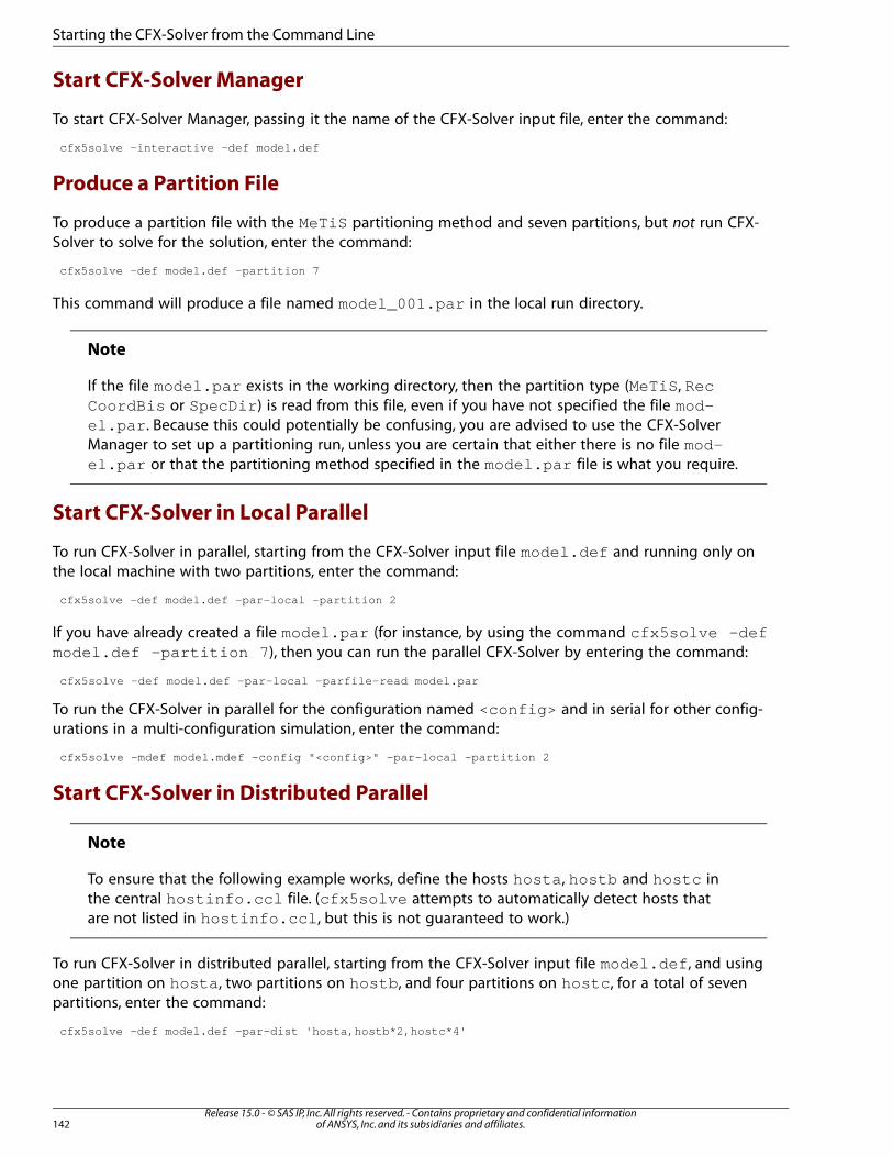
Start CFX-Solver Manager
To start CFX-Solver Manager, passing it the name of the CFX-Solver input file, enter the command:
cfx5solve -interactive -def model.def
Produce a Partition File
To produce a partition file with the MeTiS partitioning method and seven partitions, but not run CFX-Solver to solve for the solution, enter the command:
cfx5solve -def model.def -partition 7
This command will produce a file named model_001.par in the local run directory.
Note
If the file model.par exists in the working directory, then the partition type (MeTiS , RecCoordBis or SpecDir ) is read from this file, even if you have not specified the file mod-el.par . Because this could potentially be confusing, you are advised to use the CFX-SolverManager to set up a partitioning run, unless you are certain that either there is no file mod-el.par or that the partitioning method specified in the model.par file is what you require.
Start CFX-Solver in Local Parallel
To run CFX-Solver in parallel, starting from the CFX-Solver input file model.def and running only onthe local machine with two partitions, enter the command:
cfx5solve -def model.def -par-local -partition 2
If you have already created a file model.par (for instance, by using the command cfx5solve -defmodel.def -partition 7 ), then you can run the parallel CFX-Solver by entering the command:
cfx5solve -def model.def -par-local -parfile-read model.par
To run the CFX-Solver in parallel for the configuration named <config> and in serial for other config-urations in a multi-configuration simulation, enter the command:
cfx5solve -mdef model.mdef -config "<config>" -par-local -partition 2
Start CFX-Solver in Distributed Parallel
Note
To ensure that the following example works, define the hosts hosta , hostb and hostc inthe central hostinfo.ccl file. (cfx5solve attempts to automatically detect hosts thatare not listed in hostinfo.ccl , but this is not guaranteed to work.)
To run CFX-Solver in distributed parallel, starting from the CFX-Solver input file model.def , and usingone partition on hosta , two partitions on hostb , and four partitions on hostc , for a total of sevenpartitions, enter the command:
cfx5solve -def model.def -par-dist 'hosta,hostb*2,hostc*4'
Release 15.0 - © SAS IP, Inc. All rights reserved. - Contains proprietary and confidential informationof ANSYS, Inc. and its subsidiaries and affiliates.142
Starting the CFX-Solver from the Command Line
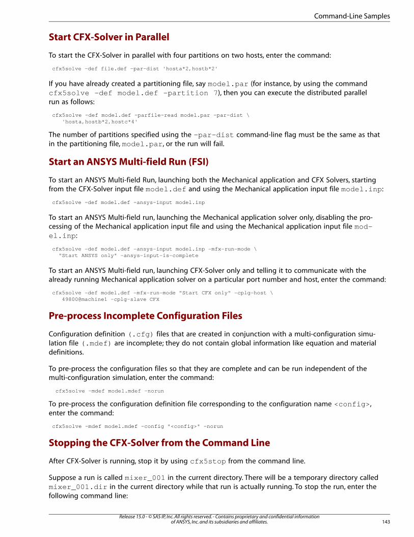
Start CFX-Solver in Parallel
To start the CFX-Solver in parallel with four partitions on two hosts, enter the command:
cfx5solve -def file.def -par-dist 'hosta*2,hostb*2'
If you have already created a partitioning file, say model.par (for instance, by using the commandcfx5solve -def model.def -partition 7 ), then you can execute the distributed parallelrun as follows:
cfx5solve -def model.def -parfile-read model.par -par-dist \ 'hosta,hostb*2,hostc*4'
The number of partitions specified using the -par-dist command-line flag must be the same as thatin the partitioning file, model.par , or the run will fail.
Start an ANSYS Multi-field Run (FSI)
To start an ANSYS Multi-field Run, launching both the Mechanical application and CFX Solvers, startingfrom the CFX-Solver input file model.def and using the Mechanical application input file model.inp :
cfx5solve -def model.def -ansys-input model.inp
To start an ANSYS Multi-field run, launching the Mechanical application solver only, disabling the pro-cessing of the Mechanical application input file and using the Mechanical application input file mod-el.inp :
cfx5solve -def model.def -ansys-input model.inp -mfx-run-mode \ "Start ANSYS only" -ansys-input-is-complete
To start an ANSYS Multi-field run, launching CFX-Solver only and telling it to communicate with thealready running Mechanical application solver on a particular port number and host, enter the command:
cfx5solve -def model.def -mfx-run-mode "Start CFX only" -cplg-host \ 49800@machine1 -cplg-slave CFX
Pre-process Incomplete Configuration Files
Configuration definition (.cfg) files that are created in conjunction with a multi-configuration simu-lation file (.mdef) are incomplete; they do not contain global information like equation and materialdefinitions.
To pre-process the configuration files so that they are complete and can be run independent of themulti-configuration simulation, enter the command:
cfx5solve -mdef model.mdef -norun
To pre-process the configuration definition file corresponding to the configuration name <config> ,enter the command:
cfx5solve -mdef model.mdef -config "<config>" -norun
Stopping the CFX-Solver from the Command Line
After CFX-Solver is running, stop it by using cfx5stop from the command line.
Suppose a run is called mixer_001 in the current directory. There will be a temporary directory calledmixer_001.dir in the current directory while that run is actually running. To stop the run, enter thefollowing command line:
143Release 15.0 - © SAS IP, Inc. All rights reserved. - Contains proprietary and confidential information
of ANSYS, Inc. and its subsidiaries and affiliates.
Command-Line Samples

cfx5stop -directory mixer_001.dir
Release 15.0 - © SAS IP, Inc. All rights reserved. - Contains proprietary and confidential informationof ANSYS, Inc. and its subsidiaries and affiliates.144
Starting the CFX-Solver from the Command Line
Chapter 12: CFX-Solver Start Methods
CFX-Solver Start Methods define allowable parameters and command-line arguments used by CFX-Solver Manager and CFX-Solver Script to launch the CFX-Solver executable and perform a run. Thedefinition of the solver start methods are modifiable by expert users to customize solver start-up forspecific parallel or batch queuing environments.
The standard start methods for a CFX installation are contained in the <CFXROOT>/etc/start-methods.ccl file. These can be over-ridden by placing a custom version of this file in the same locationas the site or user CFX configuration files.
Direct Start Methods
Solver start methods that directly run the CFX-Solver executable are known as Direct start methods,and are commonly used for defining solver execution in serial or parallel on local networks. Definitionof solver start methods for specific parallel environments can be made following the various availableMPI and PVM (UNIX only) methods in the file.
Indirect Start Methods
Solver start methods can also be used to launch a user-defined script or program that can performsystem interaction before re-executing a cfx5solve command under a different environment or system.These are known as indirect start methods, and are commonly used for executing CFX-Solver runs onremote or batch queuing systems. Use of Indirect start methods requires knowledge of a systemscripting language (such as bash or Perl) to customize the solve start-up process for your specific envir-onment. Currently the only supported indirect start method is the "Submit to Windows CCS or HPCQueue" method.
145Release 15.0 - © SAS IP, Inc. All rights reserved. - Contains proprietary and confidential information
of ANSYS, Inc. and its subsidiaries and affiliates.

Release 15.0 - © SAS IP, Inc. All rights reserved. - Contains proprietary and confidential informationof ANSYS, Inc. and its subsidiaries and affiliates.146
Chapter 13: CPU and Memory Requirements
This chapter provides information on typical increases in CPU (central processing unit) time and memoryrequirements incurred by some simulations and physical models:
13.1.Tetrahedral Mesh13.2. Special Partitioner, Solver and Interpolator Executables13.3.Turbulence13.4. Energy Models13.5. CHT Regions13.6. Multicomponent Flows13.7. Multiphase Flows13.8. Additional Variables, Wall Distance Variables, and Boundary Distance Variables13.9. Combustion Modeling13.10. Radiation Modeling13.11. GGI Interfaces13.12.Transient Runs13.13. Mesh Deformation13.14. Bidirectional (Two-Way) Couplings with ANSYS Multi-field
13.1. Tetrahedral Mesh
The ratio of elements to nodes is approximately 5:1 for a tetrahedral mesh. For example, if 5 milliontetrahedral elements are in a mesh, then there are approximately 1 million nodes. This is in contrast toa hexahedral mesh where the ratio of elements to nodes approaches 1:1 as the grid becomes large.
Memory required for a tetrahedral mesh is about 0.4 times the memory required for a hex mesh of thesame number of elements. Alternatively a tetrahedral mesh has about 2 times the required memory ofa hexahedral mesh with the same number of nodes.
13.2. Special Partitioner, Solver and Interpolator Executables
On all systems there are default Partitioner, Solver and Interpolator executables. On some systems, thereare additional executables. There are currently two classes of special executables:
• Double-Precision Executables (p. 147)
• Large Problem Partitioner Executables (p. 148)
Double-Precision Executables
Double-precision executables store basic floating point numbers as 64 bit words. These executables areavailable to permit more accurate numerical mathematical operations. Double precision accuracy mightbe needed if the computational domain involves a huge variation in grid dimension, aspect ratio,pressure range, and so on.
When double precision is used, the computer memory used for a given problem and grid size is doublethat of the default (single precision) executable. Stated another way: the maximum problem size to run
147Release 15.0 - © SAS IP, Inc. All rights reserved. - Contains proprietary and confidential information
of ANSYS, Inc. and its subsidiaries and affiliates.
on a given computer for the double precision executable is half that of the default single precision ex-ecutable.
Large Problem Partitioner Executables
This special executable is only available on 64-bit platforms. The standard partitioner is currently limitedto allocate 2^31-1 words of 4 byte integer stack space; this limits the maximum problem size for parti-tioning to approximately 80 million elements (structured) and 200 million elements (unstructured).
As a workaround, larger problems can be partitioned with the large problem partitioner. This executableinternally uses 8 byte integer data to perform the partitioning process. In theory, a maximum problemsize of 2 billion elements can be partitioned with this executable. However, practical considerations,such as available computer resources, will still limit the maximum size.
13.3. Turbulence
The following topics will be discussed:
• Zero Equation Model (p. 148)
• Two-Equation Models (p. 148)
• Reynolds Stress Model (p. 148)
Zero Equation Model
The use of this model incurs a small increase in CPU time and memory requirements compared tolaminar flow.
Two-Equation Models
Two additional scalar equations are solved when using two-equation turbulence models. The SSTmodel has a slight additional cost over other two-equation models because a wall-scale equation isalso solved.
Consider the case of single-phase, single-component laminar flow in which the U-Mom, V-Mom, W-Mom, and P-Mass equations are solved. Expect a CPU cost increase on the order of 50% by the additionof a two-equation turbulence model. Memory requirement increases are small.
Reynolds Stress Model
This model adds six scalar equations for each of the Reynolds Stresses as well as the Eddy Dissipationequation. It is approximately 2.5 times more expensive than the two-equation turbulence models.
Consider the case of single phase, single component laminar flow in which the U-Mom, V-Mom, W-Mom,and P-Mass equations are solved. Expect a CPU cost increase on the order of 120% by the addition ofa Reynolds Stress turbulence model. Memory requirement increases are small.
13.4. Energy Models
Both the thermal and total energy models require the solution of an additional scalar equation. Thesolution of the energy equation typically requires 1/3 of the CPU required for the U-Mom, V-Mom, W-Mom, and P-Mass equations. Memory requirement increases are small.
Release 15.0 - © SAS IP, Inc. All rights reserved. - Contains proprietary and confidential informationof ANSYS, Inc. and its subsidiaries and affiliates.148
CPU and Memory Requirements
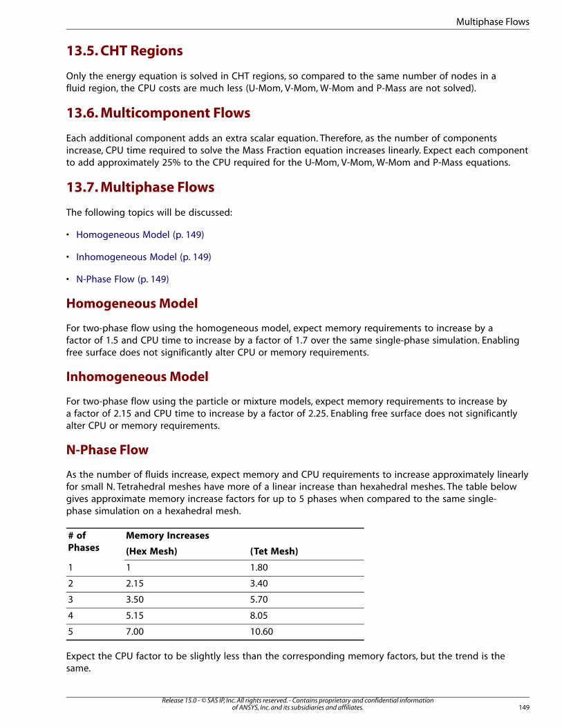
13.5. CHT Regions
Only the energy equation is solved in CHT regions, so compared to the same number of nodes in afluid region, the CPU costs are much less (U-Mom, V-Mom, W-Mom and P-Mass are not solved).
13.6. Multicomponent Flows
Each additional component adds an extra scalar equation. Therefore, as the number of componentsincrease, CPU time required to solve the Mass Fraction equation increases linearly. Expect each componentto add approximately 25% to the CPU required for the U-Mom, V-Mom, W-Mom and P-Mass equations.
13.7. Multiphase Flows
The following topics will be discussed:
• Homogeneous Model (p. 149)
• Inhomogeneous Model (p. 149)
• N-Phase Flow (p. 149)
Homogeneous Model
For two-phase flow using the homogeneous model, expect memory requirements to increase by afactor of 1.5 and CPU time to increase by a factor of 1.7 over the same single-phase simulation. Enablingfree surface does not significantly alter CPU or memory requirements.
Inhomogeneous Model
For two-phase flow using the particle or mixture models, expect memory requirements to increase bya factor of 2.15 and CPU time to increase by a factor of 2.25. Enabling free surface does not significantlyalter CPU or memory requirements.
N-Phase Flow
As the number of fluids increase, expect memory and CPU requirements to increase approximately linearlyfor small N. Tetrahedral meshes have more of a linear increase than hexahedral meshes. The table belowgives approximate memory increase factors for up to 5 phases when compared to the same single-phase simulation on a hexahedral mesh.
Memory Increases# of
Phases (Tet Mesh)(Hex Mesh)
1.8011
3.402.152
5.703.503
8.055.154
10.607.005
Expect the CPU factor to be slightly less than the corresponding memory factors, but the trend is thesame.
149Release 15.0 - © SAS IP, Inc. All rights reserved. - Contains proprietary and confidential information
of ANSYS, Inc. and its subsidiaries and affiliates.
Multiphase Flows
13.8. Additional Variables, Wall Distance Variables, and Boundary Dis-
tance Variables
A single scalar equation is added for each Additional Variable. A single scalar equation is also addedwhenever the Wall Distance variables or Boundary Distance variables are referenced in a CFX ExpressionLanguage (CEL) expression, or when these quantities are required for a built-in model (for example,two equation-turbulence or boundary-distance-based mesh-stiffness models). Note that Wall Distancevalues and Boundary Distance values are derived from the solutions of the Wall Scale equations andBoundary Scale equations, respectively. Detailed information on the wall scale equation is available atWall and Boundary Distance Formulation in the CFX-Solver Theory Guide.
Expect a CPU cost increase of approximately 20% for each Additional Variable over the solution of theU-Mom, V-Mom, W-Mom, and P-Mass equations for a single-phase single-component case. Increases inmemory requirements are small.
13.9. Combustion Modeling
Modeling combustion incurs a slight cost compared to multicomponent flow with the same numberof components. For multi-step reactions each component is solved using the coupled solve. This incursadditional CPU time that does not increase linearly with the number of components.
13.10. Radiation Modeling
This adds a single scalar equation. Cost increases are similar to those of the energy equation. For details,see Energy Models (p. 148).
13.11. GGI Interfaces
An intersection algorithm that is performed at the start of a simulation to connect each side of a GGIconnection incurs a one-time cost.
Each GGI connection means approximately 5% more CPU time and memory is required. This numbercan vary greatly, as it is a function of the number of nodes involved in a GGI connection, compared tothe number of nodes that are not involved in the GGI connection. There is also a dependence on thegeometric complexity of the GGI connection.
13.12. Transient Runs
Each coefficient loop requires approximately the same CPU time as the equivalent steady-state iteration.
13.13. Mesh Deformation
Mesh deformation using either of the Regions of Motion Specified or Junction BoxRoutine options introduces several CPU intensive operations during each outer iteration or time step.When deformation is performed using Regions of Motion Specified , a Mesh Displacementequation is assembled and solved at the start of each outer iteration or time step for Steady State andTransient simulations, respectively, and the mesh coordinates are updated. When deformation is per-formed using a Junction Box Routine , you define how mesh coordinates are updated.
After updating the mesh coordinates, other mesh related quantities (such as volumes, areas, meshquality measures, mesh velocities, and so on) are updated, and GGIs are re-intersected before advancing
Release 15.0 - © SAS IP, Inc. All rights reserved. - Contains proprietary and confidential informationof ANSYS, Inc. and its subsidiaries and affiliates.150
CPU and Memory Requirements
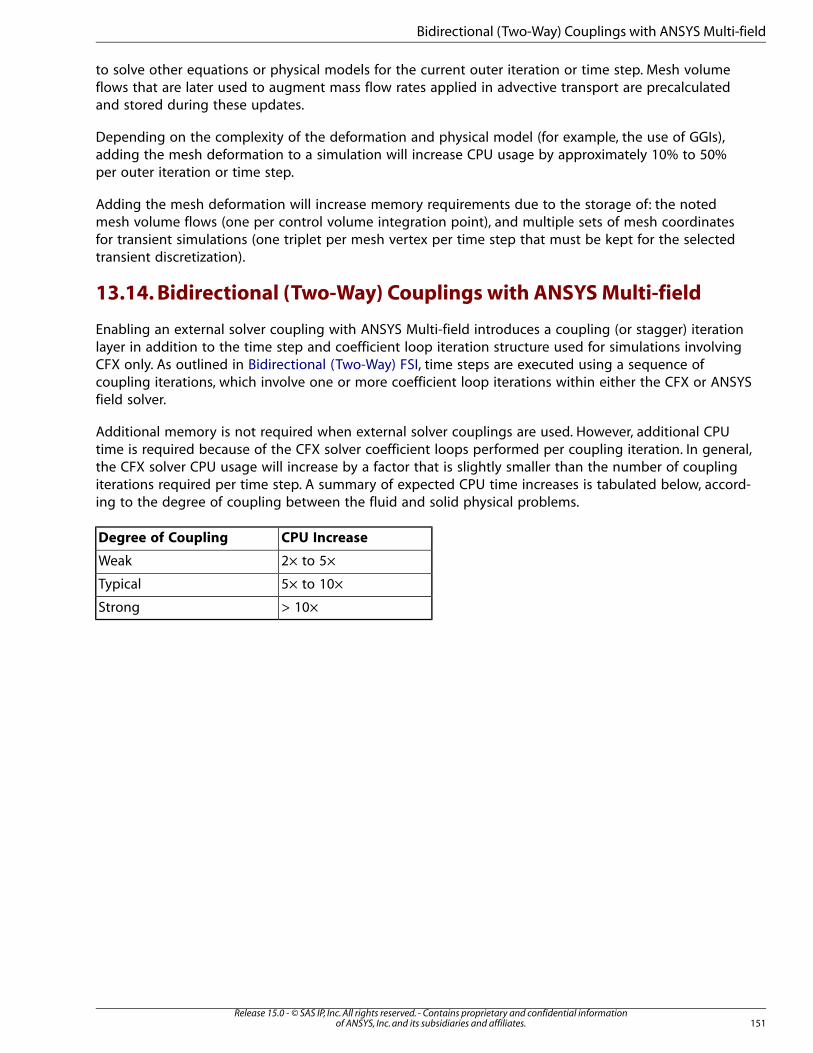
to solve other equations or physical models for the current outer iteration or time step. Mesh volumeflows that are later used to augment mass flow rates applied in advective transport are precalculatedand stored during these updates.
Depending on the complexity of the deformation and physical model (for example, the use of GGIs),adding the mesh deformation to a simulation will increase CPU usage by approximately 10% to 50%per outer iteration or time step.
Adding the mesh deformation will increase memory requirements due to the storage of: the notedmesh volume flows (one per control volume integration point), and multiple sets of mesh coordinatesfor transient simulations (one triplet per mesh vertex per time step that must be kept for the selectedtransient discretization).
13.14. Bidirectional (Two-Way) Couplings with ANSYS Multi-field
Enabling an external solver coupling with ANSYS Multi-field introduces a coupling (or stagger) iterationlayer in addition to the time step and coefficient loop iteration structure used for simulations involvingCFX only. As outlined in Bidirectional (Two-Way) FSI, time steps are executed using a sequence ofcoupling iterations, which involve one or more coefficient loop iterations within either the CFX or ANSYSfield solver.
Additional memory is not required when external solver couplings are used. However, additional CPUtime is required because of the CFX solver coefficient loops performed per coupling iteration. In general,the CFX solver CPU usage will increase by a factor that is slightly smaller than the number of couplingiterations required per time step. A summary of expected CPU time increases is tabulated below, accord-ing to the degree of coupling between the fluid and solid physical problems.
CPU IncreaseDegree of Coupling
2× to 5×Weak
5× to 10×Typical
> 10×Strong
151Release 15.0 - © SAS IP, Inc. All rights reserved. - Contains proprietary and confidential information
of ANSYS, Inc. and its subsidiaries and affiliates.
Bidirectional (Two-Way) Couplings with ANSYS Multi-field

Release 15.0 - © SAS IP, Inc. All rights reserved. - Contains proprietary and confidential informationof ANSYS, Inc. and its subsidiaries and affiliates.152
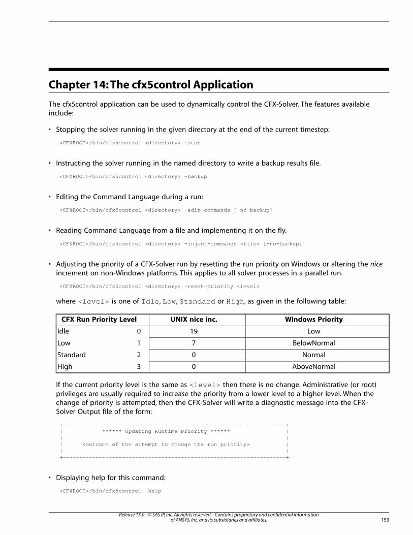
Chapter 14: The cfx5control Application
The cfx5control application can be used to dynamically control the CFX-Solver. The features availableinclude:
• Stopping the solver running in the given directory at the end of the current timestep:
<CFXROOT>/bin/cfx5control <directory> -stop
• Instructing the solver running in the named directory to write a backup results file.
<CFXROOT>/bin/cfx5control <directory> -backup
• Editing the Command Language during a run:
<CFXROOT>/bin/cfx5control <directory> -edit-commands [-no-backup]
• Reading Command Language from a file and implementing it on the fly.
<CFXROOT>/bin/cfx5control <directory> -inject-commands <file> [-no-backup]
• Adjusting the priority of a CFX-Solver run by resetting the run priority on Windows or altering the nice
increment on non-Windows platforms. This applies to all solver processes in a parallel run.
<CFXROOT>/bin/cfx5control <directory> -reset-priority <level>
where <level> is one of Idle , Low, Standard or High , as given in the following table:
Windows PriorityUNIX nice inc.CFX Run Priority Level
Low190Idle
BelowNormal71Low
Normal02Standard
AboveNormal03High
If the current priority level is the same as <level> then there is no change. Administrative (or root)privileges are usually required to increase the priority from a lower level to a higher level. When thechange of priority is attempted, then the CFX-Solver will write a diagnostic message into the CFX-Solver Output file of the form:
+--------------------------------------------------------------------+| ****** Updating Runtime Priority ****** || || <outcome of the attempt to change the run priority> || |+--------------------------------------------------------------------+
• Displaying help for this command:
<CFXROOT>/bin/cfx5control -help
153Release 15.0 - © SAS IP, Inc. All rights reserved. - Contains proprietary and confidential information
of ANSYS, Inc. and its subsidiaries and affiliates.

In these examples:
• <CFXROOT> is the path to your installation of CFX
• <directory> specifies a directory in which the ANSYS CFX solver is currently running, such as StaticMix-er_004.dir.
• -no-backup prevents the solver from writing a backup file before reading the new Command Languagefile.
Release 15.0 - © SAS IP, Inc. All rights reserved. - Contains proprietary and confidential informationof ANSYS, Inc. and its subsidiaries and affiliates.154
The cfx5control Application
Chapter 15: File Export Utility
The ANSYS CFX results file generated by a CFX-Solver run contains the details of the mesh used toperform the calculation as well as details of the results variables that have been calculated. For detailson which variables an ANSYS CFX results file contains, see List of Field Variables.
To post-process an ANSYS CFX results file using software other than CFD-Post, the mesh and variablescan be extracted from the ANSYS CFX results file into a format compliant with that 3rd party software.ANSYS CFX provides predefined translations to a number of different post-processors and analysispackages, and CFX-Solver Manager provides an interface to enable easy translation to these formats. Acommand line utility, cfx5export , can be used to perform the same operations in batch mode.
The standard file formats that can be generated from ANSYS CFX are suitable for direct input into thefollowing software systems:
• ANSYS Multi-field
• All systems that support CGNS files
• MSC.Patran, from the MacNeal-Schwendler Corporation
• FIELDVIEW, from Intelligent Light
• EnSight, from Computational Engineering International, Inc.
It is also possible to write to other formats by creating a customized export program. See Creating aCustomized Export Program.
When using CFX-Solver Manager, it is possible to export the results of a CFX-Solver run by selectingeither Tools > Export to ANSYS Multifield (see Export to ANSYS Multi-field Solver Dialog Box (p. 155))or Tools > Export (see Export of Results to Other Formats (p. 157)).
This chapter describes:15.1. Export to ANSYS Multi-field Solver Dialog Box15.2. Export of Results to Other Formats15.3. Generic Export Options15.4. Running cfx5export from the Command Line15.5. Exporting a Transient Results File15.6. Exporting Particle Tracking Data15.7. Using a Customized Export Program
Alternatively, it is possible to export the results directly from the command line. For details, see Runningcfx5export from the Command Line (p. 172).
15.1. Export to ANSYS Multi-field Solver Dialog Box
The Export to ANSYS Multifield Solver dialog box is used to produce ANSYS .cdb files for use inFluid Structure Interaction cases. To display the dialog box, select Tools > Export to ANSYS Multifield.
155Release 15.0 - © SAS IP, Inc. All rights reserved. - Contains proprietary and confidential information
of ANSYS, Inc. and its subsidiaries and affiliates.
The sections that follow describe the Export Options fields on the dialog box.
15.1.1. ANSYS Element Type
Selections correspond to the type of ANSYS element to export. The choices are:
• 3D Thermal (element type 70)
• 2D Thermal (element type 152)
• 2D Stress (element type 154).
Refer to the Mechanical APDL Theory Reference in the Mechanical APDL Theory Reference for a descriptionof these element types.
15.1.2. Output Modifiers
The following scaling and offset factors can be used to change the units of the solution. The factorscan be applied when you need to convert the units that are written to the CFX file into those that youwant to use in ANSYS.
The available modifiers are:
• Offset Flow (p. 156)
• Offset Values (p. 156)
• Scale Flow (p. 156)
• Scale Values (p. 156)
15.1.2.1. Offset Flow
Default Value: 0
Requires a real number corresponding to the offset value applied to solution flows.
15.1.2.2. Offset Values
Default Value: 0
Requires a real number corresponding to the offset value applied to solution values.
15.1.2.3. Scale Flow
Default Value: 1
Requires a real number corresponding to the scaling factor applied to solution flows.
15.1.2.4. Scale Values
Default Value: 1
Requires a real number corresponding to the scaling factor applied to solution values.
Release 15.0 - © SAS IP, Inc. All rights reserved. - Contains proprietary and confidential informationof ANSYS, Inc. and its subsidiaries and affiliates.156
File Export Utility
15.2. Export of Results to Other Formats
To export CFX-Solver result to formats such as CGNS, EnSight, FIELDVIEW, MSC.Patran, or another cus-tomized format, select Tools > Export Results from the menu bar of CFX-Solver Manager. The followingsection details the common options that can be used when exporting results to the standard formatssupported by ANSYS CFX.
15.3. Generic Export Options
To configure data for export, the Export dialog box must be displayed: select Tools > Export Results.
There are numerous export options when writing to the supported 3rd-party formats:
• Results File (p. 157)
• Domain Selection: Name (p. 157)
• Timestep Selection: Timestep (p. 157)
• Output Format (p. 157)
• Export File (p. 170)
• Output Only Boundary Geometry and Results (p. 170)
• Mesh Options: Use Initial Mesh for Rotating Domains (p. 170)
• Results Options: Output Level (p. 171)
• Results Options: Include Variables Only Found on Boundaries (p. 171)
• Results Options: Use Corrected Boundary Node Data (p. 171)
15.3.1. Results File
The name of the CFX-Solver results file to be exported.
15.3.2. Domain Selection: Name
The domain or domains in the CFX-Solver results file that are to be exported.
15.3.3. Timestep Selection: Timestep
For transient CFX-Solver results files, the timestep to be exported.
15.3.4. Output Format
Default Value: CGNS
The output format selects which standard file format the output file will be written in. If a nonstandardformat is required, select Custom User Export.
157Release 15.0 - © SAS IP, Inc. All rights reserved. - Contains proprietary and confidential information
of ANSYS, Inc. and its subsidiaries and affiliates.
Generic Export Options
The sections that follow describe the available output formats.
Note
For simulations with multiple configurations, *.mres files cannot be exported by the CFX-Solver Manager.
15.3.4.1. CGNS
The CFD General Notation System (CGNS) is designed to facilitate the exchange of data between sitesand applications, and to help stabilize the archiving of data. The data is stored in a compact, binaryformat.
CGNS consists of a collection of conventions for the storage and retrieval of CFD data. The systemconsists of two parts:
• A standard format in which the data is recorded.
• Software that reads, writes, and modifies data in that format.
Note
To configure this option, select Tools > Export. The dialog box uses numerous commonexport options. For details, see Generic Export Options (p. 157).
This section contains:
• CGNS Options (p. 158)
• Exported Files (p. 159)
• Contents of CGNS Files Written by ANSYS CFX (p. 159)
• Reading Exported Files into a Program Supporting CGNS (p. 161)
15.3.4.1.1. CGNS Options
The following options are available when writing a file in CGNS format:
• All options specified in Generic Export Options (p. 157)
• Geometry Output Only
– Default Value: Cleared.
– If selected, only mesh information and boundary condition information is written to the destinationfile; result variables are not written.
• Version and File Format
– 2.4
The ADF file format will be used in this case.
Release 15.0 - © SAS IP, Inc. All rights reserved. - Contains proprietary and confidential informationof ANSYS, Inc. and its subsidiaries and affiliates.158
File Export Utility
– 3.0
You can select either the ADF or HDF5 format.
• When Write Transient Data to One File is selected, all transient data (grid and results) are written to oneCGNS file using BaseIterativeData_t and ZoneIterativeData_t nodes within the file. Whenthis option is not selected, transient results are exported to a separate file for each timestep.
• Output boundaries as
– Default Value: Nodes
– If Nodes are selected, all boundary conditions are written as collections of nodes; if Faces, thenboundary conditions are written as groups of 2D elements (faces).
• When Use CGNS Variable Names is selected ANSYS CFX variable names are mapped to CGNS variablenames. For example Total Pressure becomes PressureStagnation .
• When Write Full CFX Solver Name as Description is selected, CFX-Solver will write a description of thefull CFX Solver Variable Name. This description is an extra data field that is used by CFD-Post when it exists.This avoids the internal variable names being used when the full CFX Solver name exceeds 32 characters.
Whenever the name of the variable exceeds 32 characters, the internal name for the variable, whichis shorter but more cryptic, is written instead. When Write Full CFX Solver Name as Description isselected, CGNS files written by CFX-Solver Manager use a new additional data tag that is not subjectto the 32-character limit, and that holds the ANSYS CFX Solver Name for each variable. CFD-Postreads the new tag in preference to the old tag, if the new tag exists.
15.3.4.1.2. Exported Files
The exported file set consists of either a single file for non-transient results, or multiple files for transientresults. Each contains a complete mesh and flow solution. By default all files are generated with a .cgnsextension. Import into a program that reads CGNS files should be done according to the importingprogram’s instructions.
ANSYS CFX-Export is capable of writing CGNS version 2.4 files in ADF format and version 3.0 files inboth ADF and HDF5 format. These CGNS files can be read by third parties if they support the featuresCFX writes and are using CGNS Version 2.0 and above.
15.3.4.1.3. Contents of CGNS Files Written by ANSYS CFX
The file produced contains grid and solution data. It does not contain problem setup (physics) inform-ation.
The amount of solution data and the type of grid written to the CGNS file is user controllable either onthe command line or via the user interface. What is seen in the CGNS file reflects what you request.There are files that when written using some options may not be able to be reread into CFX-Pre. Cautionmust therefore be used if the original CFX solution files are deleted, as it may not be possible to recoverall information.
Names of variables, zones, and boundary conditions are always CGNS-compliant. The name seen withinthe CFX application may have to be changed to achieve this. To ensure that the variable names areconsistent between CFX and CGNS files, an additional data tag is written for all solution variables,starting in CFX Release 14.0. This tag, named Ansys CFX Solver Name , is exempt from a 32-char-
159Release 15.0 - © SAS IP, Inc. All rights reserved. - Contains proprietary and confidential information
of ANSYS, Inc. and its subsidiaries and affiliates.
Generic Export Options
acter limit on variable names, so that the variable names displayed in CFD-Post match those in theresults file.
The remainder of this sections describes the data records that are written when creating a CGNS filefrom ANSYS CFX.
15.3.4.1.3.1. Base (Base_t)
A single base is written to each CGNS file.
• Its name is not significant.
• It is always written with a cell_dimension of 3 (that is, 3D).
If a transient file is being written, a simulation type (SimulationType_t ) of TimeAccurate isspecified below the base node.
A state (ReferenceState_t ) is also written below the base node with a description of where thefile was generated from and what it represents.
15.3.4.1.3.2. Zones (Zone_t)
A single zone is written under each Base_t node for each domain you requested and is always unstruc-tured in nature.
Coordinates of node data are always written in double precision. Due to the nature of the grid beingunstructured, there is no implicit ordering in how the grid is written.
15.3.4.1.3.3. Elements (Elements_t)
Element sections are written on a one per domain/subdomain basis as well as a one per boundarycondition basis. Due to the nature of CFX data, a single element cannot appear in more than one elementsection. Element numbering is unique and consecutive.
You can control whether volume mesh (with surface mesh) or a surface mesh is written to the file.
15.3.4.1.3.4. Boundary Conditions (BC_t)
Boundary Conditions are written. The location of each boundary condition is specified as set of 2Delements (faces) or a set of nodes. The former is generally preferred as the latter can have some restric-tions for the program that reads the file.
No properties of the boundary condition are written other than its type.
15.3.4.1.3.5. Solution Data (FlowSolution_t)
Solution data is written where requested. Names are mapped to be CGNS compliant. No discrete datais currently written. Where Wall Only data is present, “missing” solution data is written as 0.0.
15.3.4.1.3.6. Transient Data
Transient data is written to separate CGNS files by writing the Grid and Solution data for each CFXtransient file that is available to the cfx5export process.
Release 15.0 - © SAS IP, Inc. All rights reserved. - Contains proprietary and confidential informationof ANSYS, Inc. and its subsidiaries and affiliates.160
File Export Utility
15.3.4.1.3.7. ANSYS CFX Connectivity using CGNS for Aerodynamic Noise Analysis
Further information on exporting files is contained in Aerodynamic Noise Analysis in the CFX-Solver
Modeling Guide.
15.3.4.1.4. Reading Exported Files into a Program Supporting CGNS
There is a wide range of products that can import CGNS files. Consult user documentation for theproduct being used for further information.
Note
An issue was detected while reading a CGNS file in TecPlot 10 and earlier that prevented thefiles written by ANSYS CFX being read by TecPlot. If a problem is encountered, try settingthe environment variable CFX5_EXPORT_CGNS_TECPLOT to a value of 1, restart ANSYS CFX,and export the CGNS file again. If the problem persists, contact either ANSYS support orTecPlot support.
15.3.4.2. MSC.Patran
MSC.Patran is a general-purpose CAE simulation tool.
Note
To configure this option, select Tools > Export. The dialog box uses numerous commonexport options. For details, see Generic Export Options (p. 157).
This section contains:
• Available Options (p. 161)
• Exported Files (p. 162)
• Reading Exported Files into MSC.Patran (p. 162)
• Exporting Boundary Conditions to MSC.Patran (p. 163)
• Example Procedure (p. 163)
15.3.4.2.1. Available Options
The following options are available when writing a file in MSC.Patran format:
• All options specified in Generic Export Options (p. 157)
• Geometry Output Only (Neutral File)
– Default Value: Cleared.
If selected, the mesh from the ANSYS CFX results file is written to a Neutral file; solution variablesare not written to the Neutral file. For more details about MSC.Patran Neutral files, refer to yourdocumentation from MSC.Patran.
161Release 15.0 - © SAS IP, Inc. All rights reserved. - Contains proprietary and confidential information
of ANSYS, Inc. and its subsidiaries and affiliates.
Generic Export Options
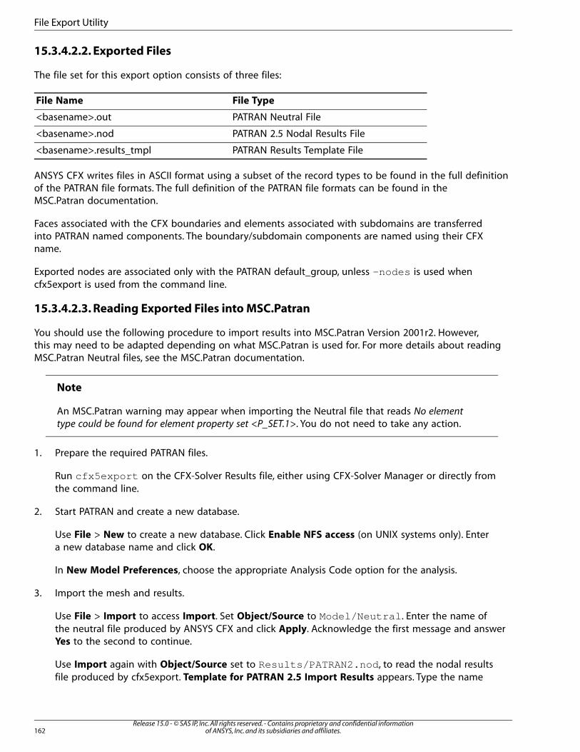
15.3.4.2.2. Exported Files
The file set for this export option consists of three files:
File TypeFile Name
PATRAN Neutral File<basename>.out
PATRAN 2.5 Nodal Results File<basename>.nod
PATRAN Results Template File<basename>.results_tmpl
ANSYS CFX writes files in ASCII format using a subset of the record types to be found in the full definitionof the PATRAN file formats. The full definition of the PATRAN file formats can be found in theMSC.Patran documentation.
Faces associated with the CFX boundaries and elements associated with subdomains are transferredinto PATRAN named components. The boundary/subdomain components are named using their CFXname.
Exported nodes are associated only with the PATRAN default_group, unless -nodes is used whencfx5export is used from the command line.
15.3.4.2.3. Reading Exported Files into MSC.Patran
You should use the following procedure to import results into MSC.Patran Version 2001r2. However,this may need to be adapted depending on what MSC.Patran is used for. For more details about readingMSC.Patran Neutral files, see the MSC.Patran documentation.
Note
An MSC.Patran warning may appear when importing the Neutral file that reads No element
type could be found for element property set <P_SET.1>. You do not need to take any action.
1. Prepare the required PATRAN files.
Run cfx5export on the CFX-Solver Results file, either using CFX-Solver Manager or directly fromthe command line.
2. Start PATRAN and create a new database.
Use File > New to create a new database. Click Enable NFS access (on UNIX systems only). Entera new database name and click OK.
In New Model Preferences, choose the appropriate Analysis Code option for the analysis.
3. Import the mesh and results.
Use File > Import to access Import. Set Object/Source to Model/Neutral . Enter the name ofthe neutral file produced by ANSYS CFX and click Apply. Acknowledge the first message and answerYes to the second to continue.
Use Import again with Object/Source set to Results/PATRAN2.nod , to read the nodal resultsfile produced by cfx5export. Template for PATRAN 2.5 Import Results appears. Type the name
Release 15.0 - © SAS IP, Inc. All rights reserved. - Contains proprietary and confidential informationof ANSYS, Inc. and its subsidiaries and affiliates.162
File Export Utility
of the template file produced by cfx5export and click OK. Enter the nodal results file name in Importand click Apply.
4. Continue to use MSC.Patran as required.
15.3.4.2.4. Exporting Boundary Conditions to MSC.Patran
CFX can be used to provide data to be used as boundary conditions for other types of analysis inMSC.Patran.
MSC.Patran enables models to be prepared for several different kinds of analysis. It also has facilitiesfor using imported data to define data fields suitable for interpolating loads and boundary conditionsonto the geometry or the mesh of a new model.
A description of the relevant PATRAN facilities, in particular the Fields function and its applications,can be found in the MSC.Patran documentation.
15.3.4.2.5. Example Procedure
Here is an outline of some guidelines for one possible procedure for incorporating CFX results into aPATRAN model. CFX temperature predictions will be used to define a temperature distribution on ageometry surface of a new model. Details about any of the options can be found in the MSC.Patrandocumentation.
Points to note in this example are:
• Files generated by ANSYS CFX should be read into a new database first before any PATRAN model grid.This ensures that the node numbers of the Neutral file correspond to the nodal result file. The nodes andelements in the new model mesh will be numbered or renumbered to follow on from those in the CFXdata.
• The CFX model should not be included in the new model analysis, but the CFX data must not be deleteduntil the boundary values have been interpolated onto the new grid.
The example assumes exported results include the Temperature variable.
1. Prepare PATRAN Neutral and Nodal results files containing boundary data only.
Export the ANSYS CFX results file to MSC.Patran format, either using CFX-Solver Manager or directlyfrom the command line. Toggle Boundary Data Output Only on if using CFX-Solver Manager, oruse the -boundary option if using cfx5export from the command line.
2. Start PATRAN and create a new database.
Use File > New to create a new database. Click Enable NFS access (on UNIX systems only). Entera new database name and click OK.
On New Model Preferences, choose the appropriate Analysis Code option, for example, PATRAN2 NF .
3. Import the mesh and results.
Use File > Import. Set Object/Source to Model/Neutral . Enter the name of the Neutral fileproduced by ANSYS CFX and click Apply. Acknowledge the message to continue.
163Release 15.0 - © SAS IP, Inc. All rights reserved. - Contains proprietary and confidential information
of ANSYS, Inc. and its subsidiaries and affiliates.
Generic Export Options
Use Import again with Object/Format set to Results/PATRAN2.nod , to read the nodal resultsfile produced by ANSYS CFX. Template for PATRAN 2.5 Import Results appears. Enter the nameof the template file produced by ANSYS CFX, and click OK. Enter the nodal results file name andclick Apply.
4. Display temperature results as a fringe plot.
Select Group/Post to post just the group containing the boundary condition nodes to use. SelectResults. On Results, select the temperature results, and click Apply.
5. Create a continuous FEM field from the displayed variable.
Select the Fields option. Set Action/Object/Method to Create/Spatial/FEM . Enter a newname under Field Name. Click the Continuous option. Select the relevant group underMesh/Results Group Filter. Click Apply.
6. Add the geometry for the new model.
Post the default_group and make it current using Group/Post. Use the toolbar icons to ensure thedisplay will be in wireframe mode rather than in hidden line mode. Then either create a geometryfor the new PATRAN model using the Geometry option to open the Geometry form or import thegeometry from a previously prepared database using File > Import with Object/Source set toModel/ MSC/PATRAN DB .
7. Define a temperature boundary condition on new geometry surfaces.
Select the Load/BCs option. Set Action/Object/Type to Create/Temperature/Nodal . Entera name under New Set Name. Click Input Data. Select the field in the Spatial Fields box and clickOK. Under Load/Boundary Conditions, click Select Application Region to display Select Applic-
ation Region. Click the Geometry option under Geometry Filter. In Select Geometric Entities,pick the surfaces to apply the boundary condition to. Click Add and then OK. In Load/Boundary
Conditions, click Apply. A temperature distribution should now be visible on the relevant geometrysurfaces, in the form of values shown at the intersections of the surface display lines.
8. Complete the PATRAN model.
15.3.4.3. FIELDVIEW
FIELDVIEW is a stand-alone CFD post processor supplied by Intelligent Light.
Note
To configure this option, select Tools > Export. The dialog box uses numerous commonexport options. For details, see Generic Export Options (p. 157).
This section contains:
• Available Options (p. 165)
• Exported Files (p. 165)
• Reading Exported Files in FIELDVIEW (p. 166)
Release 15.0 - © SAS IP, Inc. All rights reserved. - Contains proprietary and confidential informationof ANSYS, Inc. and its subsidiaries and affiliates.164
File Export Utility
15.3.4.3.1. Available Options
The following options are available when writing a file for use in FIELDVIEW Unstructured format:
• All Options specified in Generic Export Options (p. 157).
• FV-UNS File Options: The options in this section detail the formatting of the separate grid and resultsfiles or combined grid and results files that are written in FV-UNS (FIELDVIEW Unstructured) file format.
• Version:
– Default Value: 3.0
– The value selected details which version of the format should be used when writing the grid and resultsto files for use within FIELDVIEW. You should use the most recent version of the file format supportedby your FIELDVIEW installation. Refer to the FIELDVIEW documentation for this information.
• Split Grid and Results Format:
– Default Value: Selected
– When selected, the grid from the ANSYS CFX results file is written to one file and the results to a secondor subsequent files. If not selected, a single combined file is written containing both the grid and theresults.
Note
→This option is not available when the version is less than 2.7.
→If the number of variables that are to be written to the file exceeds 200, the results willbe written to more than one results file. Refer to FIELDVIEW 9 and later to learn how toload multiple files into FIELDVIEW.
• Format:
– Default Value: Unstructured Binary
– This option enables a choice of whether the FV-UNS are written as in binary or ASCII format. The ASCIIformat is human-readable but larger than the binary format. It is therefore recommended by ANSYSand FIELDVIEW that binary format files be written in most cases.
• FV-REG Version:
– Default Value: 2.0
– The version specified here details the version of the format used when writing the region file for usein FIELDVIEW. You should specify the highest version that is supported by the version of FIELDVIEWyou have installed.
15.3.4.3.2. Exported Files
The file set for this export option consists of several files, depending on the format options selected.
165Release 15.0 - © SAS IP, Inc. All rights reserved. - Contains proprietary and confidential information
of ANSYS, Inc. and its subsidiaries and affiliates.
Generic Export Options
If the output format is selected to be Split Grid and Results Format, more than one file will be generatedwith the grid in one file and results in at least one other. Optionally, a region file will also be generated:
File TypeFile Name
FIELDVIEW Grid File<basename>_grid.fv
FIELDVIEW Results File<basename>_results.fv
FIELDVIEW Region File<basename>_region.fv
If Split Grid and Results Format (see Available Options (p. 165)) is not selected, then at least onecombined grid and results file will be generated:
File TypeFile Name
FIELDVIEW Combined Grid and Res-ults File
<basename>.fv
FIELDVIEW Region File<basename>_grid.fv.fvreg
Optionally, if particle tracks have been written in the ANSYS CFX results file, then these will be writtento one or more FIELDVIEW particle track files:
File TypeFile Name
FIELDVIEW Particle Track File<basename>_n.fv
ANSYS CFX writes a subset of record types that are available in the full FIELDVIEW file formats. Thedocumentation supplied with FIELDVIEW describes all the record types that can be read by differentversions of FIELDVIEW.
15.3.4.3.3. Reading Exported Files in FIELDVIEW
Files can be read into EnSight 5, 6, 7, and 8 as required:
• FIELDVIEW Versions 10.1 and Later (p. 166)
• FIELDVIEW Versions 9 and 10 (p. 167)
• FIELDVIEW Versions 6, 7, 8 (p. 167)
15.3.4.3.3.1. FIELDVIEW Versions 10.1 and Later
If the exported file is split into more than one file, it is necessary to follow a procedure similar to thefollowing to read each file in FIELDVIEW:
1. Select File > Data Input > ANSYS-CFX[FV-UNS Export]….
2. On the ANSYS-CFX[FV-UNS Export] form, ensure that the INPUT MODE is Replace .
3. If the file written is in Split Grid and Results format:
a. Click Read Grid or Combined Data.
b. Select the grid file from the file popup and click OK.
c. Click Read Results Data.
Release 15.0 - © SAS IP, Inc. All rights reserved. - Contains proprietary and confidential informationof ANSYS, Inc. and its subsidiaries and affiliates.166
File Export Utility
d. Select the first results file and click OK.
e. If further grid or results files are to be loaded, change the INPUT MODE to Append on the ANSYS-
CFX[FV-UNS Export] form and repeat from step “a” until all grid or results files have been loaded.
4. If the file is a combined file:
a. Click Read Grid or Combined Data.
b. Select the combined file from the file popup and click OK.
15.3.4.3.3.2. FIELDVIEW Versions 9 and 10
If the exported file is split into more than one file, it is necessary to follow a procedure similar to thefollowing to read each file in FIELDVIEW:
1. Select File > Data Input > Unstructured.
2. On the FV Unstructured form ensure that the INPUT MODE is Replace .
3. If the file written is in Split Grid and Results format:
a. Click Read Grid or Combined Data.
b. Select the grid file from the file popup and click OK.
c. Click Read Results Data.
d. Select the first results file and click OK.
e. If further grid or results files are to be loaded, change the INPUT MODE to Append on the FV
Unstructured form and repeat from step “a” until all grid or results files have been loaded.
4. If the file is a combined file:
a. Click Read Grid or Combined Data.
b. Select the combined file from the file popup and click OK.
15.3.4.3.3.3. FIELDVIEW Versions 6, 7, 8
The following procedure enables importing results into FIELDVIEW Version 6, 7 and 8.
Note
FIELDVIEW reads the version number from within the input file; however, some file formatsthat can be generated by ANSYS CFX cannot be read by all version of FIELDVIEW. Refer toFIELDVIEW documentation for exact details of which file formats can be processed byFIELDVIEW.
167Release 15.0 - © SAS IP, Inc. All rights reserved. - Contains proprietary and confidential information
of ANSYS, Inc. and its subsidiaries and affiliates.
Generic Export Options
1. Select Data Files > Unstructured Data Input from the menu bar. In File Selection, select the file createdusing cfx5export and then click OK. In Function Subset Selection, select All and click OK. Click Exit
in Unstructured Data Input.
2. The results can now be analyzed as required.
Note
The Region file written by ANSYS CFX to these versions of FIELDVIEW may have to be modifiedto ensure correct axes of rotation and rotational velocities in FIELDVIEW.
If the ANSYS CFX file contains multiple rotation axes, it is not possible to write a singleFIELDVIEW file that can be correctly used in FIELDVIEW. In this case, you must write the filein “Split Grid and Results Format”. For more details about reading FIELDVIEW Unstructuredfiles, see the FIELDVIEW documentation.
15.3.4.4. EnSight
EnSight is a suite of tools for engineering and scientific simulation.
Note
To configure this option, select Tools > Export. The dialog box uses numerous commonexport options. For details, see Generic Export Options (p. 157).
This section contains:
• Available Options (p. 168)
• Export Files (p. 169)
• Reading Exported Files into EnSight (p. 169)
15.3.4.4.1. Available Options
The following options are available when writing files for use in EnSight:
• All options specified in Generic Export Options (p. 157)
• EnSight Version:
– Default Value: Gold
– The selection specifies the EnSight file format version to which the output will adhere. It is recommendedthat Gold be selected wherever possible. Refer to the EnSight documentation for differences betweenthe different formats.
• Format:
– Default Value: Unstructured Binary
Release 15.0 - © SAS IP, Inc. All rights reserved. - Contains proprietary and confidential informationof ANSYS, Inc. and its subsidiaries and affiliates.168
File Export Utility

– This option enables you to choose whether the EnSight data files are written as in binary or ASCII format.The ASCII format is human-readable but larger than the binary format. It is therefore recommended byANSYS that binary format files are written in most cases.
15.3.4.4.2. Export Files
The file set for this export option consists of the following files:
File TypeFile Name
EnSight Geometry File<basename>.geom
EnSight Results File (version 5 only)<basename>.results
EnSight Variable Files for scalar variable<basename>.s01 (and so on)
EnSight Variable Files for vector variables<basename>.v01 (and so on)
EnSight case files (EnSight 6 and later).<basename>.case
Note
• Each subdomain and boundary condition is exported as one EnSight part.
• CFX variable aliases have to be modified (by removing spaces and special characters and bylimiting the name length) to create valid EnSight variable names. In some cases the names thatresult may not be human recognizable; in all cases the mapping from the name used in ANSYSCFX to that written to the EnSight file is displayed in the progress window of the Solver Manager.
ANSYS CFX uses a subset of record types that are available in the full EnSight file formats. The docu-mentation supplied with EnSight describes all the record types that can be used.
15.3.4.4.3. Reading Exported Files into EnSight
Files can be read into EnSight 5, 6, 7, and 8 as required.
• EnSight 8.2 and Later (p. 169)
• EnSight 6, 7, and 8.0 (p. 170)
• EnSight 5 (p. 170)
15.3.4.4.3.1. EnSight 8.2 and Later
The following procedure enables importing results into EnSight 8.2 and later. For more details aboutimporting, see the EnSight documentation.
1. Select File > Open.
2. Select the Format as Case .
3. Choose the case file that has been exported. All files produced by CFX-Solver Manager are automaticallyloaded.
169Release 15.0 - © SAS IP, Inc. All rights reserved. - Contains proprietary and confidential information
of ANSYS, Inc. and its subsidiaries and affiliates.
Generic Export Options
15.3.4.4.3.2. EnSight 6, 7, and 8.0
The following procedure enables importing results into EnSight 6, 7, or 8.0. Results files may needmodification, depending on how they are to be used with EnSight. For more details about importing,see the EnSight documentation.
1. Select File > Data Reader.
2. Select the Format as Case .
3. Choose the case file that has been exported. All files produced by CFX-Solver Manager are automaticallyloaded.
15.3.4.4.3.3. EnSight 5
The following procedure enables importing results into EnSight 5. Results files may need modification,depending on how they are to be used with EnSight. For more details about importing, see the EnSightdocumentation.
1. Select File > Data (Reader). In File Selection, click the name of the geometry file created usingcfx5export, and then click (Set) Geometry.
2. Click the name of the EnSight results file. Click (Set) Result and then click Okay.
3. In Data Part Loader, click Load All, and then click Close.
4. The results can now be analyzed as required.
15.3.4.5. Custom User Export
Files can be exported to a custom format from CFX-Solver Manager. To do so, a custom export programmust be created. For information on all the ways of using a custom export program, see Using a Cus-tomized Export Program (p. 177). For details on creating a custom export program, see Creating a Cus-tomized Export Program.
15.3.5. Export File
This option specifies the destination file to which the grid and results will be written. This file namemay be altered in such a way that multiple files may be written with transient data or if the OutputFormat requires multiple files to be written.
15.3.6. Output Only Boundary Geometry and Results
Availability: All Standard Formats (CGNS, MSC.Patran, FIELDVIEW and EnSight). Available only whenGeometry Output Only is not selected.
Default Value: Not selected.
If selected, only the data for nodes on the boundaries is output. This can be used, for example, to enableresults from CFD calculations to provide boundary conditions for other analysis in other packages.
15.3.7. Mesh Options: Use Initial Mesh for Rotating Domains
Availability: All Standard Formats (CGNS, MSC.Patran, FIELDVIEW and EnSight)
Release 15.0 - © SAS IP, Inc. All rights reserved. - Contains proprietary and confidential informationof ANSYS, Inc. and its subsidiaries and affiliates.170
File Export Utility
Default Value: Not selected.
By default, the mesh for any rotating domain is rotated into the correct position for the timestep whenexporting, as long as the angular velocity is specified as a single value (that is, not using the CFX Expres-sion Language). You can choose to always write the mesh as it was positioned at the initial timestepby selecting the option Use Initial Mesh for Rotating Domains.
If the angular velocity of the rotating domain is specified in terms of an expression, then the mesh isalways exported in its initial position and never rotated, and the Use Initial Mesh for Rotating Domains
option is ignored.
The calculation of the correct rotated position assumes that the initial run was started from a time valueof 0 [s], and that the simulation time is continuous from 0 [s] through every run and restart (that is, theInitial Time is not reset by using the Value option). If this is not the case, then you should select Use
Initial Mesh for Rotating Domains option to write the mesh as it was positioned at the initial timestep,to avoid incorrectly rotated meshes.
15.3.8. Results Options: Output Level
Availability: All Standard Formats (CGNS, MSC.Patran, FIELDVIEW and EnSight)
Default Value: 1.
The output level selects a predefined subset of variables to write to the destination results file. Eachvariable is given a “user level” by CFX-Solver. For details, see List of Field Variables.
An output level of:
• 1 writes a small subset of basic variables such as velocity and pressure, which have user level 1.
• 2 writes all variables that are of user levels 1 and 2.
• 3 writes all variables stored in the CFX results file.
15.3.9. Results Options: Include Variables Only Found on Boundaries
Availability: All Standard Formats (CGNS, MSC.Patran, FIELDVIEW and EnSight)
Default Value: Not selected.
If selected, the variables that exist only on boundaries (such as +� ) are written in addition to those
variables that have values in the interior of the domain(s).
15.3.10. Results Options: Use Corrected Boundary Node Data
Availability: All Standard Formats (CGNS, MSC.Patran, FIELDVIEW and EnSight)
Default Value: Selected
The values of some variables on the boundary nodes (that is, on the edges of the geometry) are notprecisely equal to the specified boundary conditions when CFX-Solver finishes calculations.
For instance, the value of velocity on a node on the wall will not be precisely zero, and the value oftemperature on an inlet may not be precisely the specified inlet temperature. For visualization purposes,
171Release 15.0 - © SAS IP, Inc. All rights reserved. - Contains proprietary and confidential information
of ANSYS, Inc. and its subsidiaries and affiliates.
Generic Export Options
it can be more helpful if the nodes at the boundary contain the specified boundary conditions and soUse Corrected Data on Boundary Nodes should be selected for these cases.
Corrected boundary node values are obtained by taking the results produced by CFX-Solver (called“conservative values”) and overwriting the results on the boundary nodes with the values specified bythe boundary conditions set up in CFX-Pre. This ensures, for example, that velocity is displayed as zeroon no-slip walls and is equal to the specified inlet velocity on an inlet. Using corrected boundary nodevalues is equivalent to selecting conservative variables as described in Hybrid and Conservative VariableValues in the CFX Reference Guide.
15.4. Running cfx5export from the Command Line
In the following code, [ ] denotes an optional argument, and <> and # denote that substitution ofa suitable value is required. All other arguments are keywords, some of which may have a short form.
Note
-cgns , -ensight , -fieldview , -patran , or -custom should be the first option onthe command line.
• -cgns creates files suitable for an application that supports the CGNS format.
• -ensight creates files suitable for input into the EnSight post-processor.
• -patran creates files suitable for input into the MSC/PATRAN post-processor.
• -fieldview creates files suitable for input into the FIELDVIEW post-processor.
• -custom should be used if there is a need for custom-defined export formats. For details, see Runninga Customized Export Program using cfx5export from the Command Line (p. 178).
For all standard options (-cgns , -patran , -fieldview , and -ensight ), the source ANSYS CFX file<file> is the same file as would be specified under Tools > Export > Results File in CFX-SolverManager. The optional file entered as -name <file> is the filename used as the basename for thefiles generated as part of the export process (this is equivalent to what is specified under Tools > Export
> Export File).
15.4.1. Running cfx5export
To run cfx5export from the command line, type one of the following commands into a UNIX terminalor a suitable Windows command line and press Return or Enter. For details, see Command Line in theCFX Reference Guide.
cfx5export -ansysfsi [-domain <number>] [-help] [-name <file>] \ [-offset-flow <number>] [-offset-val <number>] \ [-scale-flow <number>] [-scale-val <number>] \ [-summary] [-timestep <number>] [-verbose] \ [-eltype <element type>] [-regions <region1><,region2>...] <file>
or
cfx5export -cgns [-boundary] [-corrected] [-domain <number>] \ [-cgns-version <2.4|3.0>] [-HDF5|-ADF] \ [-geometry] [-help] [-include] [-name <file>] [-summary] \ [-timestep <number>] [-user <level>] [-norotate] \ [-boundaries-as-nodes|-boundaries-as-faces] \
Release 15.0 - © SAS IP, Inc. All rights reserved. - Contains proprietary and confidential informationof ANSYS, Inc. and its subsidiaries and affiliates.172
File Export Utility
[-one-file-for-transient-cases] [-cgns-names] \ [-no-cfx-variable-description] [-verbose] <file>
or
cfx5export -ensight [-5|-6|-7] [-absolute] [-ascii|-binary] \ [-corrected] [-domain <number>] [-help] [-include] [-long] \ [-name <file>] [-summary] [-timestep <number>] [-user <level>] \ [-verbose] <file>
or
cfx5export -fieldview [-UNS[2.4|2.5|2.6|2.7|3.0]] [-REG[1.0|2.0]] \ [-absolute] [-ascii] [-corrected] [-domain <number>] [-noparticles] \ [-include] [-name <file>] [-summary] [-timestep <number>] \ [-user <level>] [-norotate] [-verbose] <file>
or
cfx5export -patran [-absolute] [-boundary] [-corrected] [-domain <number>] \ [-geometry] [-help] [-include] [-name <file>] [-nodes] [-summary] \ [-timestep <number>] [-user <level>] [-norotate] [-verbose] <file>
or
cfx5export [-exec <executable>] -custom [<options>]
15.4.2. cfx5export Arguments
A basic description of the cfx5export arguments is given below.
UsageArgument
Alternative Forms
Write an EnSight Version 5 case file instead of an EnSight Version7 results file.
-5
Write an EnSight version 6 file instead of an EnSight version 7 file.-6
Write an EnSight version 7 file (default)-7
Write CGNS data as an ADF formatted file.-adf
Export data in the ANSYS FSI CDB format.-ansysfsi
Write the output file in ASCII format, rather than unstructuredbinary format.
-ascii
-s
Write the output file in unstructured binary format.-binary
Boundary data only. Using this argument corresponds to selectingthe option Boundary Data Output Only when using cfx5exportfrom CFX-Solver Manager.
-boundary
-b
Write boundary conditions as collections of faces rather than nodes.-boundaries-as-faces
Write boundary conditions as collections of nodes rather than faces(default).
-boundaries-as-nodes
Export data in the CGNS format-cgns
Map CFX variable names to CGNS variable names (where possible).-cgns-names
173Release 15.0 - © SAS IP, Inc. All rights reserved. - Contains proprietary and confidential information
of ANSYS, Inc. and its subsidiaries and affiliates.
Running cfx5export from the Command Line
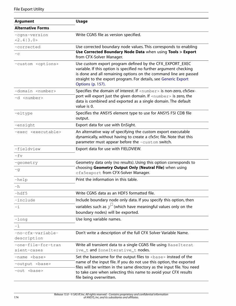
UsageArgument
Alternative Forms
Write CGNS file as version specified.-cgns-version<2.4|3.0>
Use corrected boundary node values. This corresponds to enablingUse Corrected Boundary Node Data when using Tools > Export
from CFX-Solver Manager.
-corrected
-c
Use custom export program defined by the CFX_EXPORT_EXECvariable. If this option is specified no further argument checking
-custom <options>
is done and all remaining options on the command line are passedstraight to the export program. For details, see Generic ExportOptions (p. 157).
Specifies the domain of interest. If <number> is non-zero, cfx5ex-port will export just the given domain. If <number> is zero, the
-domain <number>
-d <number>data is combined and exported as a single domain. The defaultvalue is 0.
Specifies the ANSYS element type to use for ANSYS FSI CDB fileoutput.
-eltype
Export data for use with EnSight.-ensight
An alternative way of specifying the custom export executabledynamically, without having to create a cfx5rc file. Note that thisparameter must appear before the -custom switch.
-exec <executable>
Export data for use with FIELDVIEW.-fieldview
-fv
Geometry data only (no results). Using this option corresponds tochoosing Geometry Output Only (Neutral File) when usingcfx5export from CFX-Solver Manager.
-geometry
-g
Print the information in this table.-help
-h
Write CGNS data as an HDF5 formatted file.-hdf5
Include boundary node only data. If you specify this option, then
variables such as +� (which have meaningful values only on the
boundary nodes) will be exported.
-include
-i
Use long variable names.-long
-l
Don’t write a description of the full CFX Solver Variable Name.-no-cfx-variable-description
Write all transient data to a single CGNS file using BaseIterative_t and ZoneIterative_t nodes.
-one-file-for-transient-cases
Set the basename for the output files to <base> instead of thename of the input file. If you do not use this option, the exported
-name <base>
-output <base>files will be written in the same directory as the input file. You need
-out <base> to take care when selecting this name to avoid your CFX resultsfile being overwritten.
Release 15.0 - © SAS IP, Inc. All rights reserved. - Contains proprietary and confidential informationof ANSYS, Inc. and its subsidiaries and affiliates.174
File Export Utility
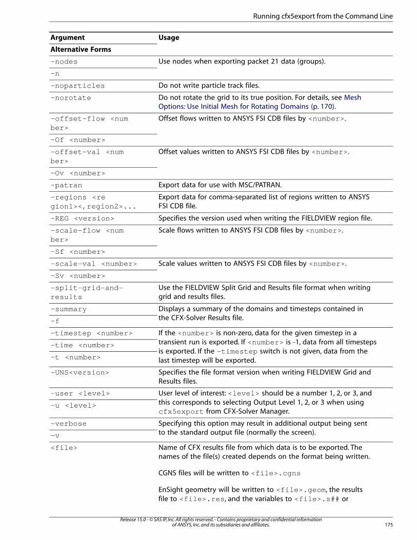
UsageArgument
Alternative Forms
Use nodes when exporting packet 21 data (groups).-nodes
-n
Do not write particle track files.-noparticles
Do not rotate the grid to its true position. For details, see MeshOptions: Use Initial Mesh for Rotating Domains (p. 170).
-norotate
Offset flows written to ANSYS FSI CDB files by <number> .-offset-flow <number>
-Of <number>
Offset values written to ANSYS FSI CDB files by <number> .-offset-val <number>
-Ov <number>
Export data for use with MSC/PATRAN.-patran
Export data for comma-separated list of regions written to ANSYSFSI CDB file.
-regions <region1><,region2>...
Specifies the version used when writing the FIELDVIEW region file.-REG <version>
Scale flows written to ANSYS FSI CDB files by <number> .-scale-flow <number>
-Sf <number>
Scale values written to ANSYS FSI CDB files by <number> .-scale-val <number>
-Sv <number>
Use the FIELDVIEW Split Grid and Results file format when writinggrid and results files.
-split-grid-and-results
Displays a summary of the domains and timesteps contained inthe CFX-Solver Results file.
-summary
-f
If the <number> is non-zero, data for the given timestep in atransient run is exported. If <number> is -1, data from all timesteps
-timestep <number>
-time <number>is exported. If the -timestep switch is not given, data from thelast timestep will be exported.-t <number>
Specifies the file format version when writing FIELDVIEW Grid andResults files.
-UNS<version>
User level of interest: <level> should be a number 1, 2, or 3, andthis corresponds to selecting Output Level 1, 2, or 3 when usingcfx5export from CFX-Solver Manager.
-user <level>
-u <level>
Specifying this option may result in additional output being sentto the standard output file (normally the screen).
-verbose
-v
Name of CFX results file from which data is to be exported. Thenames of the file(s) created depends on the format being written.
<file>
CGNS files will be written to <file>.cgns
EnSight geometry will be written to <file>.geom , the resultsfile to <file>.res , and the variables to <file>.s## or
175Release 15.0 - © SAS IP, Inc. All rights reserved. - Contains proprietary and confidential information
of ANSYS, Inc. and its subsidiaries and affiliates.
Running cfx5export from the Command Line
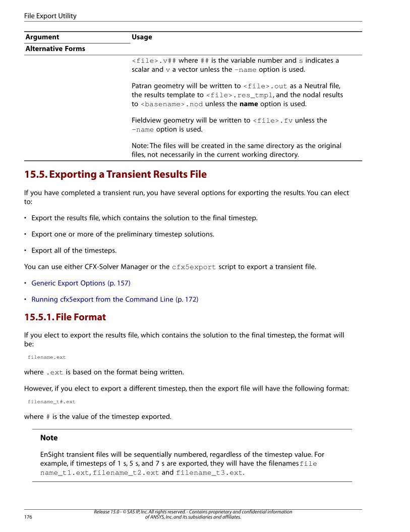
UsageArgument
Alternative Forms
<file>.v## where ## is the variable number and s indicates ascalar and v a vector unless the -name option is used.
Patran geometry will be written to <file>.out as a Neutral file,the results template to <file>.res_tmpl , and the nodal resultsto <basename>.nod unless the name option is used.
Fieldview geometry will be written to <file>.fv unless the-name option is used.
Note: The files will be created in the same directory as the originalfiles, not necessarily in the current working directory.
15.5. Exporting a Transient Results File
If you have completed a transient run, you have several options for exporting the results. You can electto:
• Export the results file, which contains the solution to the final timestep.
• Export one or more of the preliminary timestep solutions.
• Export all of the timesteps.
You can use either CFX-Solver Manager or the cfx5export script to export a transient file.
• Generic Export Options (p. 157)
• Running cfx5export from the Command Line (p. 172)
15.5.1. File Format
If you elect to export the results file, which contains the solution to the final timestep, the format willbe:
filename.ext
where .ext is based on the format being written.
However, if you elect to export a different timestep, then the export file will have the following format:
filename_t#.ext
where # is the value of the timestep exported.
Note
EnSight transient files will be sequentially numbered, regardless of the timestep value. Forexample, if timesteps of 1 s, 5 s, and 7 s are exported, they will have the filenames filename_t1.ext , filename_t2.ext and filename_t3.ext .
Release 15.0 - © SAS IP, Inc. All rights reserved. - Contains proprietary and confidential informationof ANSYS, Inc. and its subsidiaries and affiliates.176
File Export Utility
15.6. Exporting Particle Tracking Data
Export of particle tracking data is currently supported only to FIELDVIEW. Export of particle trackingdata to any other format is not supported in the current release of ANSYS CFX.
15.7. Using a Customized Export Program
There are multiple ways in which an export program can be used once it has been compiled.
• Using a Customized Export Program from CFX-Solver Manager (p. 177)
• Using a Customized Export Program from the Command Line (p. 177)
15.7.1. Using a Customized Export Program from CFX-Solver Manager
Open the Export dialog box by selecting Export from the Tools menu of CFX-Solver Manager.
1. Set Output Format to Custom User Export .
2. Supply the path to the compiled program in Export Executable.
3. Enter any associated options required to run the customized program (such as would be entered at thecommand line) in Custom Export Setting.
4. The specified custom export program runs with the associated arguments when you click Export.
15.7.2. Using a Customized Export Program from the Command Line
You may run your program directly from the command line started from the ANSYS CFX Launcher(Tools > Command Line). Such a command line will have the environment variables and path set ap-propriately.
Important
It is important to run the command line in the CFX environment. For details, see CommandLine in the CFX Reference Guide.
15.7.2.1. Running a Customized Export Program Directly from the Command Line
For the purposes of describing what you can do, assume that the executable file is called myexportand is contained in the directory /home/smith/export/ (UNIX) or c:\smith\export (Windows).You want to specify the results file called file.res in the same directory and make the basenameexample .
15.7.2.1.1. UNIX
To run the program directly on a UNIX system, open a command line started from the ANSYS CFXLauncher (Tools > Command Line) and call your program using:
./myexport file.res example
assuming that the current directory is /home/smith/export/ .
177Release 15.0 - © SAS IP, Inc. All rights reserved. - Contains proprietary and confidential information
of ANSYS, Inc. and its subsidiaries and affiliates.
Using a Customized Export Program
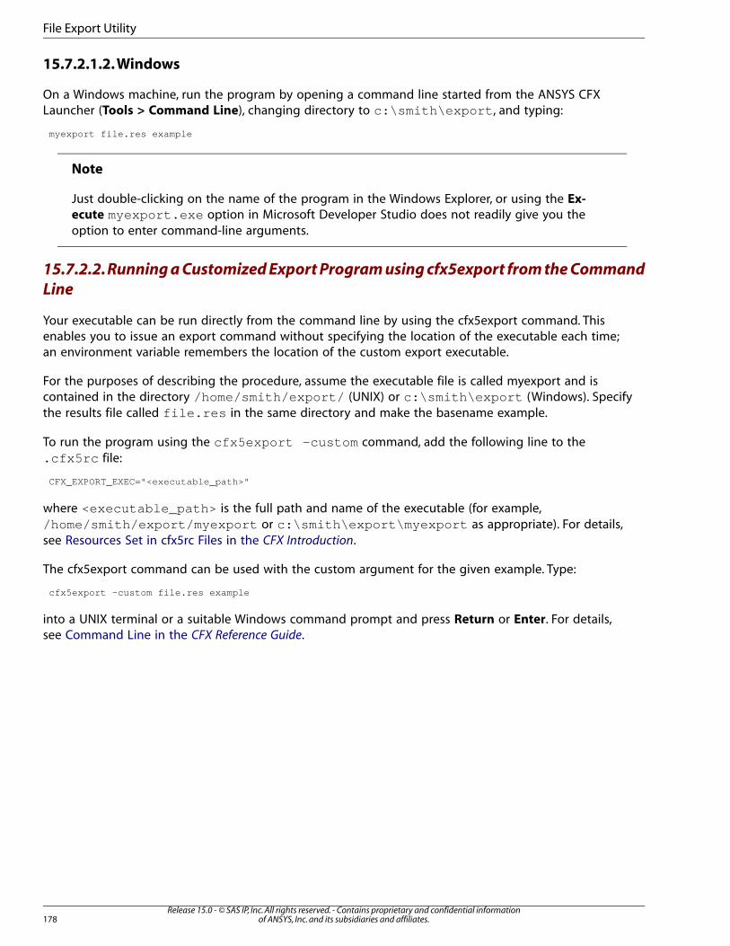
15.7.2.1.2. Windows
On a Windows machine, run the program by opening a command line started from the ANSYS CFXLauncher (Tools > Command Line), changing directory to c:\smith\export , and typing:
myexport file.res example
Note
Just double-clicking on the name of the program in the Windows Explorer, or using the Ex-
ecute myexport.exe option in Microsoft Developer Studio does not readily give you theoption to enter command-line arguments.
15.7.2.2. Running a Customized Export Program using cfx5export from the Command
Line
Your executable can be run directly from the command line by using the cfx5export command. Thisenables you to issue an export command without specifying the location of the executable each time;an environment variable remembers the location of the custom export executable.
For the purposes of describing the procedure, assume the executable file is called myexport and iscontained in the directory /home/smith/export/ (UNIX) or c:\smith\export (Windows). Specifythe results file called file.res in the same directory and make the basename example.
To run the program using the cfx5export -custom command, add the following line to the.cfx5rc file:
CFX_EXPORT_EXEC="<executable_path>"
where <executable_path> is the full path and name of the executable (for example,/home/smith/export/myexport or c:\smith\export\myexport as appropriate). For details,see Resources Set in cfx5rc Files in the CFX Introduction.
The cfx5export command can be used with the custom argument for the given example. Type:
cfx5export -custom file.res example
into a UNIX terminal or a suitable Windows command prompt and press Return or Enter. For details,see Command Line in the CFX Reference Guide.
Release 15.0 - © SAS IP, Inc. All rights reserved. - Contains proprietary and confidential informationof ANSYS, Inc. and its subsidiaries and affiliates.178
File Export Utility

Index
AAdditional Variables
CPU and memory requirements of, 150ANSYS CFX-Solver Manager
customizing, 8starting, 1
ANSYS GST and NLH variables, 112ANSYS multi-field
CPU and memory requirements of, 151ANSYS Multi-field run, 25
restarting, 30arrange workspace command, 115
Bbackground color
setting for Solver monitor, 108backup run command, 115boundary
corrected node values, 174node only data, 174
Ccatalogue size, 17CCL file
editing, 94structure, 94
CFD (Computational Fluid Dynamics)job information, 42
CFX commandscfx5export, 172cfx5interp, 123
CFX exportwith transient results, 176
CFX variablesAERODYNAMIC DAMPING, 110EFFICIENCY, 110FLOW, 110for monitoring a CFX run, 110FORCE, 110IMBALANCE, 111MOMENT, 110NEG ACCUMULATION, 111PARTICLE, 111RADIOMETER, 111RESIDUAL, 111RIGID BODY, 111SOURCE, 111TIMESTEP, 111USER POINT, 112
CFX-Solverconfiguring memory for, 17parallel run, 19pre-processing incomplete configuration files, 143run output results, 18starting an ANSYS Multi-field Run (FSI), 143starting from the command line, 129starting in distributed parallel, 142starting in local parallel, 142starting in parallel, 143stopping the CFX-Solver from the command line,143
CFX-Solver input fileeditor - rules, 93
CFX-Solver input file editorchanging appearance of, 94
CFX-Solver Managertext output window, 5
CFX-Solver Manager File menu, 99CFX-Solver Manager workspace menu commands
overview, 105CFX-Solver Manager workspace properties command
overview, 105CFX-Solver Output file
absorbed by porous media, 67collected on walls, 67command file, 39completed job information (parallel), 60computed model constants, 47conjugate heat transfer, 62continue from last time step (transient only), 67convergence history, 46, 55CPU requirements, 54entered domain, 67exceeded distance limit, 67exceeded integration limit, 68exceeded time limit, 68false transient information, 53fell below minimum diameter, 68final average scales, 53global conservation statistics, 48header, 39host information (parallel), 60initial average scales, 45integrated particle flows, 69integration error, 68job information, 42, 54job information (parallel), 59left domain, 68linear solution, 46maximum residual, 46, 52memory usage, 43
179Release 15.0 - © SAS IP, Inc. All rights reserved. - Contains proprietary and confidential information
of ANSYS, Inc. and its subsidiaries and affiliates.
memory usage (parallel), 60mesh adaption, 61mesh statistics, 43particle convergence history, 69particle fate diagnostics, 67particle transport equations, 66partitioning information (parallel), 59rate, 46rigid body, 73rms residual, 46sliding along walls, 68solved equations, 45thermal energy (solid), 62waiting for next time step (transient only), 68wall forces and moments, 51
cfx5cmds command, 94cfx5control
controls CFX-Solver run, 153cfx5export
CFX command, 172cfx5solve
command-line options, 130examples, 141starts CFX-Solver, 129
cfx5stopstops CFX-Solver, 143
CHT regionsCPU and memory requirements of, 149
close workspace command, 100combustion modeling
CPU and memory requirements of, 150command file, 39Command File Editor
overview, 89commands
close workspace, 100computed model constants, 47convergence
history, 46, 55convergence discontinuities
preventing in immersed solids runs, 115convergence history plots
for CFX-Solver Manager runs, 3printing, 4
corrected boundary node values, 174CPU requirements, 54
Ddefine run command, 99Define Run dialog box, 10distributed parallel
setup, 20
double buffering, 103double-precision executables
CPU and memory requirements of, 147
Eenergy models
CPU and memory requirements of, 148EnSight
options, 168post-processing, 155using exported files, 169
equation residual, 85export
boundary conditions to MSC/Patran, 163cfx5mondata, 5executable, 177plot data, 4transient results file, 176
Ffalse transient information, 53fieldview
post-processing, 155file
format, 176file export utility, 155Fluid Structure Interaction cases
exporting data for, 155
GGGI interfaces
CPU and memory requirements of, 150
Hhomogeneous model
CPU and memory requirements of, 149
Iimmersed solids runs
preventing convergence discontinuities, 115importing results
to Fieldview, 166information
false transient, 53inhomogeneous model
CPU and memory requirements of, 149Initial Values tab, 11interpolating results, 121Interpolator tab, 16
Llarge problem partitioner executables
Release 15.0 - © SAS IP, Inc. All rights reserved. - Contains proprietary and confidential informationof ANSYS, Inc. and its subsidiaries and affiliates.180
Index
CPU and memory requirements of, 148load layout command, 116local parallel
setup, 20
MMemory Management System (MMS)
catalogue size, 17mesh
statistics, 43mesh deformation
CPU and memory requirements of, 150mesh interpolation, 121
using command line, 123monitor finished run command, 99monitor run in progress command, 99monitors
deleting, 107general settings, 108modifying, 107plot lines, 109range settings, 108setting background color, 108
mouse mapping, 103MSC/Patran
options, 161post-processing, 155
MST filedefines a plot monitor, 117
multi-configuration Run History page, 6multi-field run, 25
restarting, 30multicomponent flows
CPU and memory requirements of, 149MultiField tab, 12multiphase flows
CPU and memory requirements of, 149
NN-phase flow
CPU and memory requirements of, 149new monitor command, 114
Ooptions
ANSYS CFX-Solver Manager, 101common, 102
Pparallel run
configuring, 20of CFX-Solver, 19
parallel run job information, 60particle transport
particle fates, 67partition file
producing, 142Partitioner tab, 13partitioning
coupled, 15information, 59viewing, 77
plot monitorcreating a new, 117shows expression values vs timestep, 106
post-processingEnSight, 155fieldview, 155MSC/Patran, 155
printingsolver convergence history, 4
priorityspecifying a renice value, 153
Rradiation modeling
CPU and memory requirements of, 150renice
adjusting the priority of a CFX-Solver run, 153reset to default workspace command, 118reset-priority
adjusting the priority of a CFX-Solver run, 153residual monitor
shows contents of text files updated during the run,106shows residual values vs timestep, 106
residual plotobtaining for old runs, 86
residual plottingoverview, 85transient, 86
restart current run command, 115restarting a run, 22results
interpolating, 121results file, 73results files
backing up, 115editing, 89
Reynolds Stress modelCPU and memory requirements of, 148
rigid bodyoutput file, 73
rules file, 96
181Release 15.0 - © SAS IP, Inc. All rights reserved. - Contains proprietary and confidential information
of ANSYS, Inc. and its subsidiaries and affiliates.
Run Definition tab, 10runs
monitoring, 114preventing discontinuities, 115restarting current, 115stopping current, 114
Ssave layout command, 116Save Settings, 9solver run
Initial Values tab, 11Interpolator tab, 16MultiField tab, 12overview, 9Partitioner tab, 13restarting, 22Run Definition tab, 10Solver tab, 16using mesh adaption, 23
Solver tab, 16stop current run command, 114surface charge, 71
Ttetrahedral mesh
CPU and memory requirements of, 147text output window
in CFX-Solver Manager, 5toggle layout type command, 116transient information
false, 53transient runs
CPU and memory requirements of, 150transient simulations
exporting data from, 176two-equation models
CPU and memory requirements of, 148
Uuser
export, 170
Vvariables
plotting by a specific, 113variables file, 96view MAX residuals command, 118view RMS residuals command, 117
WWorkspace selector
for CFX-Solver Manager runs, 2
Zzero-equation model
CPU and memory requirements of, 148
Release 15.0 - © SAS IP, Inc. All rights reserved. - Contains proprietary and confidential informationof ANSYS, Inc. and its subsidiaries and affiliates.182
Index
Related Documents