Analyzing Multivariable Change: Optimization Chapter 8.1 Extreme Points and Saddle Points.

Analyzing Multivariable Change:Optimization

Chapter 8.1Extreme Points and Saddle Points

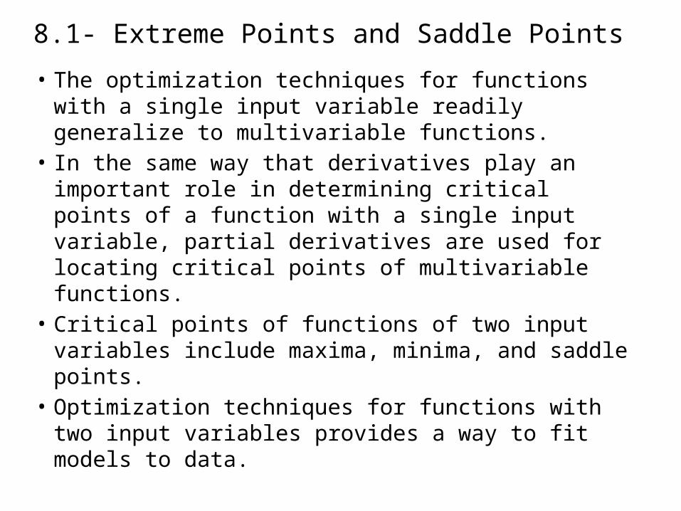
8.1- Extreme Points and Saddle Points

• The optimization techniques for functions with a single input variable readily generalize to multivariable functions.

• In the same way that derivatives play an important role in determining critical points of a function with a single input variable, partial derivatives are used for locating critical points of multivariable functions.

• Critical points of functions of two input variables include maxima, minima, and saddle points.

• Optimization techniques for functions with two input variables provides a way to fit models to data.

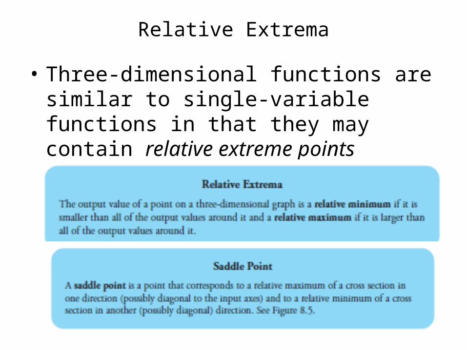
Relative Extrema

• Three-dimensional functions are similar to single-variable functions in that they may contain relative extreme points

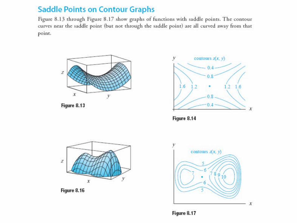
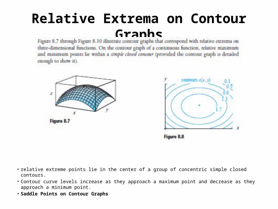
Relative Extrema on Contour Graphs

• relative extreme points lie in the center of a group of concentric simple closed contours. • Contour curve levels increase as they approach a maximum point and decrease as they approach

a minimum point.• Saddle Points on Contour Graphs

Absolute Extrema

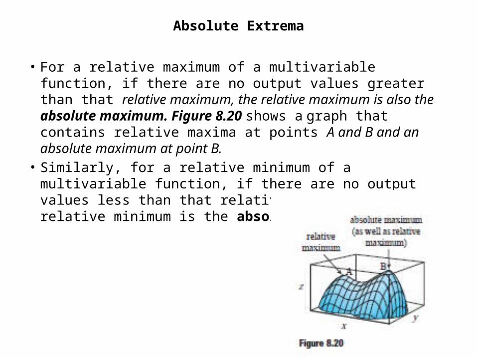
• For a relative maximum of a multivariable function, if there are no output values greater than that relative maximum, the relative maximum is also the absolute maximum. Figure 8.20 shows a graph that contains relative maxima at points A and B and an absolute maximum at point B.

• Similarly, for a relative minimum of a multivariable function, if there are no output values less than that relative minimum, that relative minimum is the absolute minimum

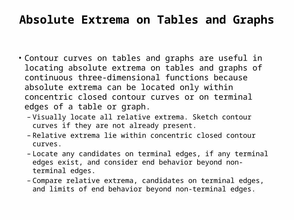
Absolute Extrema on Tables and Graphs

• Contour curves on tables and graphs are useful in locating absolute extrema on tables and graphs of continuous three-dimensional functions because absolute extrema can be located only within concentric closed contour curves or on terminal edges of a table or graph.– Visually locate all relative extrema. Sketch contour curves if they

are not already present.– Relative extrema lie within concentric closed contour curves.– Locate any candidates on terminal edges, if any terminal edges

exist, and consider end behavior beyond non-terminal edges.– Compare relative extrema, candidates on terminal edges, and

limits of end behavior beyond non-terminal edges.

Problem 4,6, 10

Analyzing Multivariable Change:Optimization

Chapter 8.2Multivariable Optimization

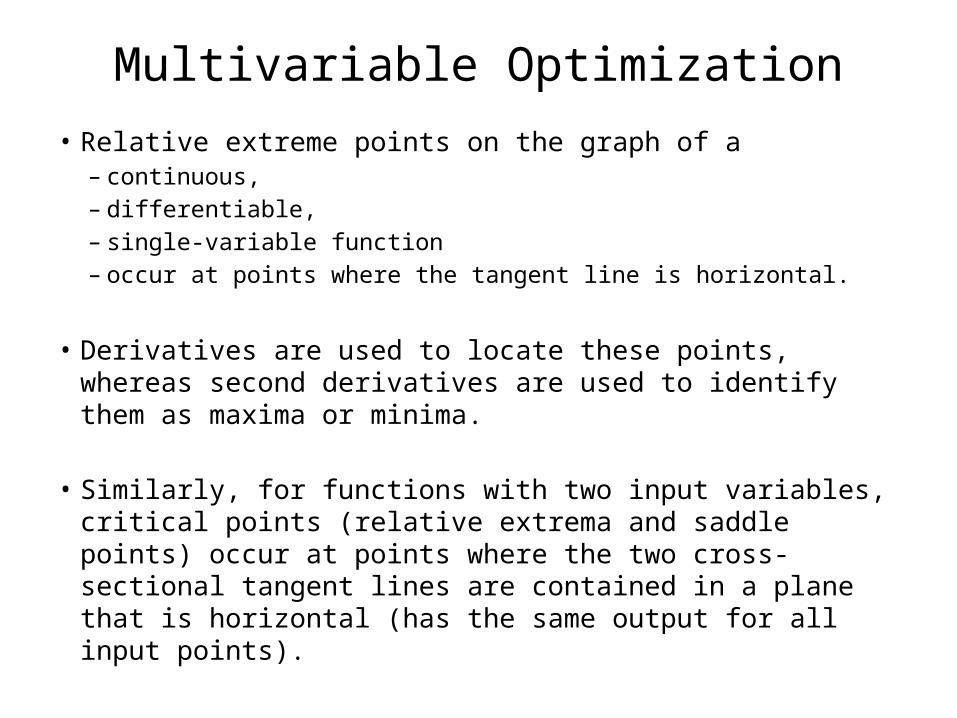
Multivariable Optimization• Relative extreme points on the graph of a

– continuous, – differentiable, – single-variable function– occur at points where the tangent line is horizontal.

• Derivatives are used to locate these points, whereas second derivatives are used to identify them as maxima or minima.

• Similarly, for functions with two input variables, critical points (relative extrema and saddle points) occur at points where the two cross-sectional tangent lines are contained in a plane that is horizontal (has the same output for all input points).

When Partial Rates of Change are Zero

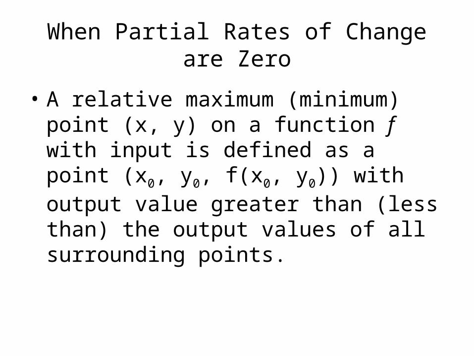
• A relative maximum (minimum) point (x, y) on a function f with input is defined as a point (x0, y0, f(x0, y0)) with output value greater than (less than) the output values of all surrounding points.

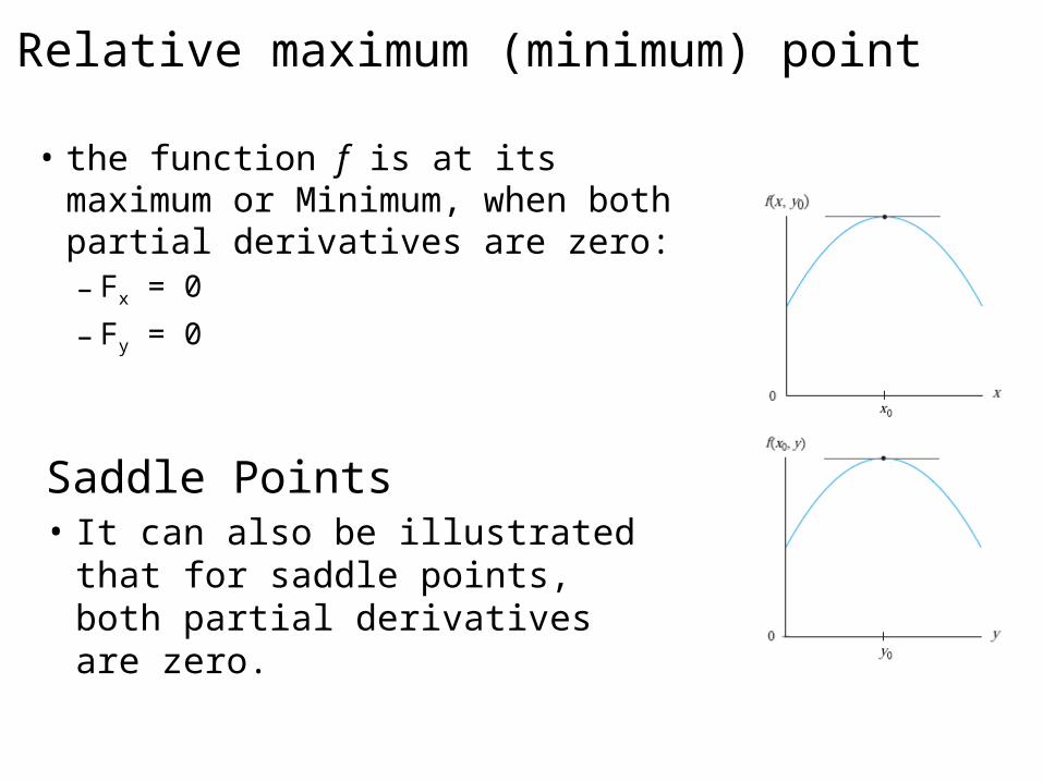
Relative maximum (minimum) point

• the function f is at its maximum or Minimum, when both partial derivatives are zero:– Fx = 0

– Fy = 0

Saddle Points• It can also be illustrated that

for saddle points, both partial derivatives are zero.

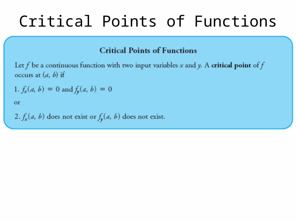
Critical Points of Functions

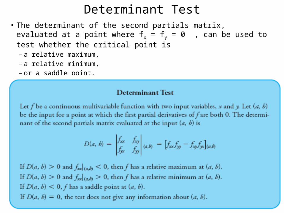
Determinant Test• The determinant of the second partials matrix, evaluated at a point

where fx = fy = 0 , can be used to test whether the critical point is – a relative maximum, – a relative minimum, – or a saddle point. – This test is known as the Determinant Test.

Problem 2, 4, 10, 12, 16, 20

Analyzing Multivariable Change:Optimization

Chapter 8.3Optimization under Constraints

Optimization under Constraints

• In many optimization applications, the context dictates constraints on what input values can be used.

• For example, when trying to optimize revenue made from the sales of a product, the producer is constrained by the total amount of product the company is able to produce.

• When a manufacturer is trying to maximize production, budget constraints must be considered.

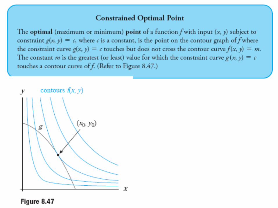
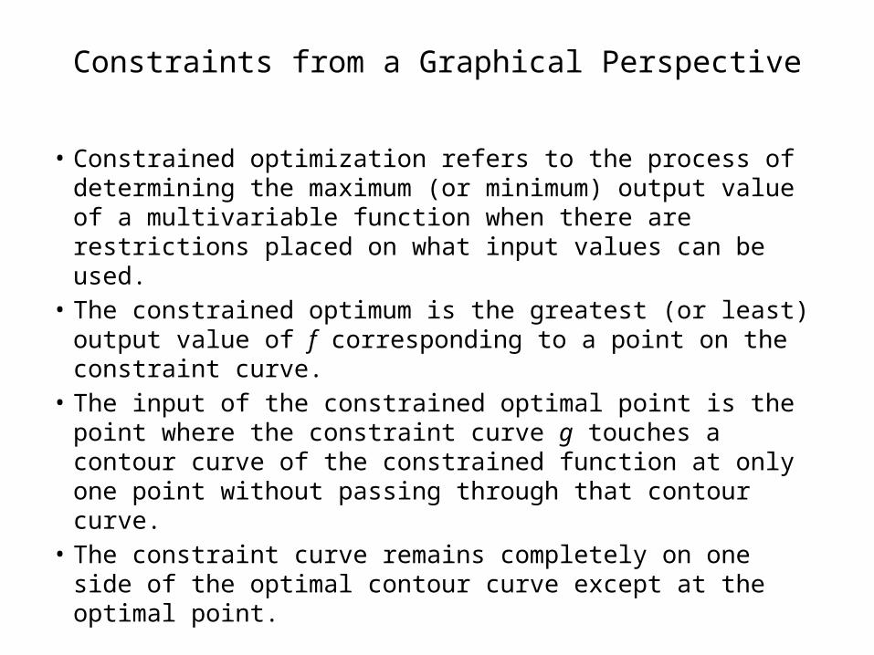
Constraints from a Graphical Perspective

• Constrained optimization refers to the process of determining the maximum (or minimum) output value of a multivariable function when there are restrictions placed on what input values can be used.

• The constrained optimum is the greatest (or least) output value of f corresponding to a point on the constraint curve.

• The input of the constrained optimal point is the point where the constraint curve g touches a contour curve of the constrained function at only one point without passing through that contour curve.

• The constraint curve remains completely on one side of the optimal contour curve except at the optimal point.

Constrained Optimal Points

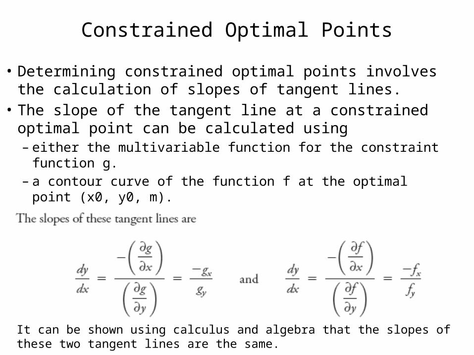
• Determining constrained optimal points involves the calculation of slopes of tangent lines.

• The slope of the tangent line at a constrained optimal point can be calculated using – either the multivariable function for the constraint function g. – a contour curve of the function f at the optimal point (x0, y0, m).

It can be shown using calculus and algebra that the slopes of these two tangent lines are the same.

Numerical Verification of a Constrained Optimum

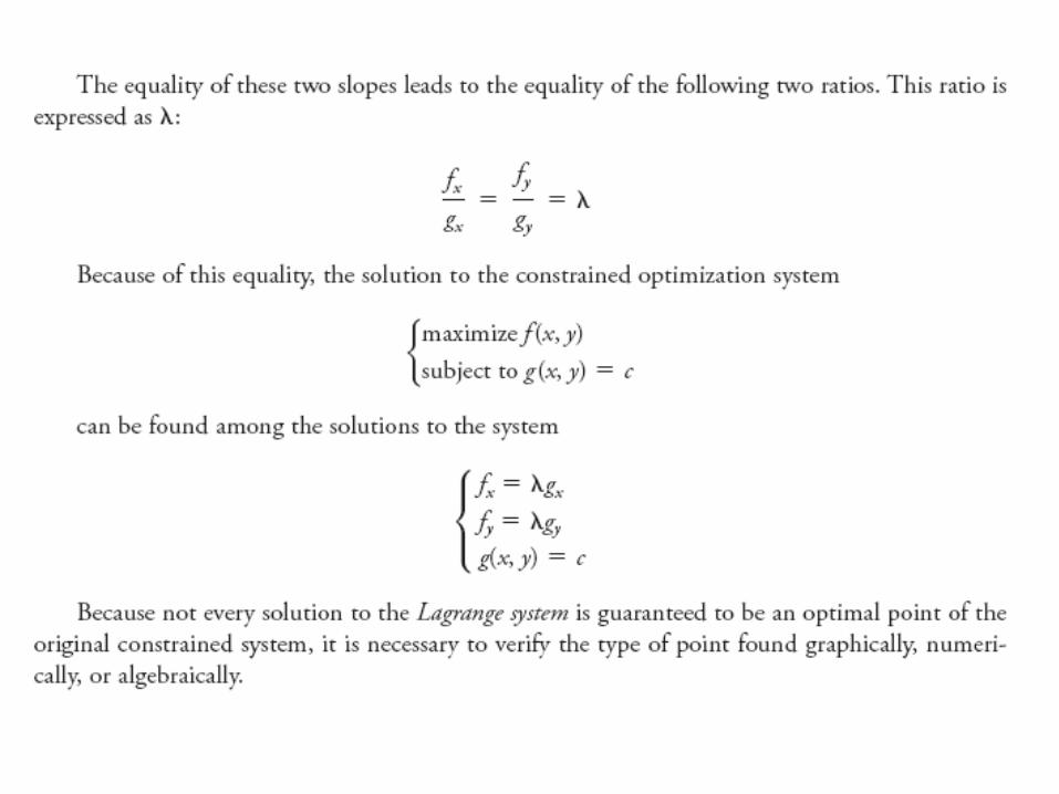
• Because not all solutions to the Lagrange system have to be optimal points of the constrained problem, it is a good idea to verify that the solution found is really an optimum.

• Verification can be done graphically, but it is often easier, faster, and more accurate to verify the optimum numerically.

• To verify numerically that a solution to the Lagrange system is the optimal point for the constrained system, check the output value of the solution point with the output value of two close points on the constrained function.

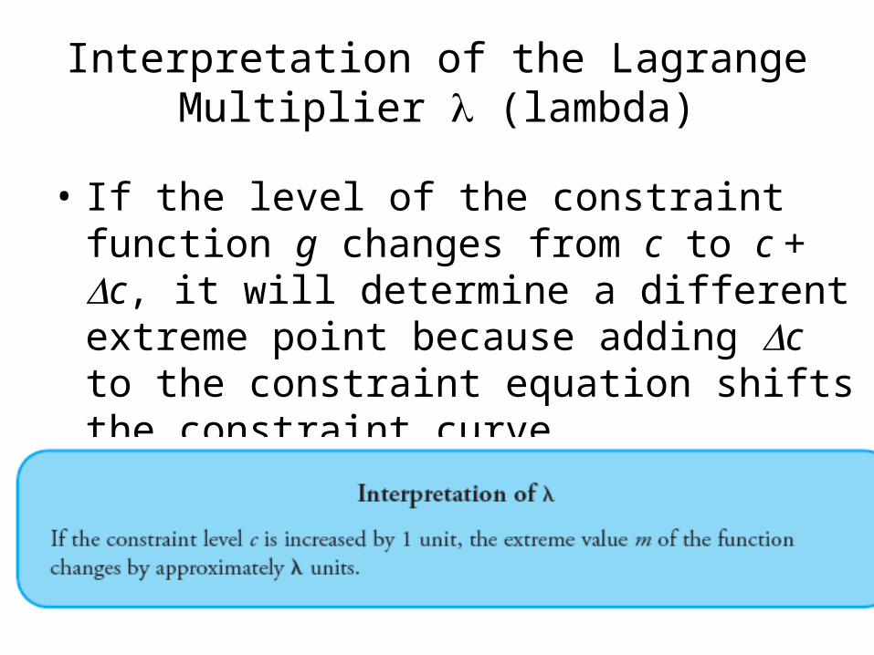
Interpretation of the Lagrange Multiplier (lambda)

• If the level of the constraint function g changes from c to c + c, it will determine a different extreme point because adding c to the constraint equation shifts the constraint curve.

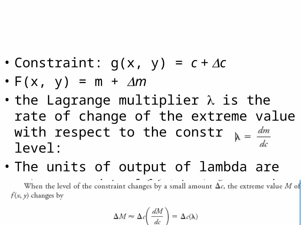
• Constraint: g(x, y) = c + c• F(x, y) = m + m• the Lagrange multiplier is the rate of change of the

extreme value with respect to the constraint level:• The units of output of lambda are– (output units of f ) per (output units of g)

Problem 6, 8, 10, 16, 22, 24