analysis of organic rankine cycles considering both expander and cycle performances angelo la seta Master’s Thesis Energy Engineering DTU Mechanichal engineering, Thermal Energy Section Ingegneria industriale e dell’informazione Corso di laurea magistrale in ingegneria energetica Matr. 787567 Anno accademico 2013/2014 November 2014 – Lyngby, København supervisors Fredrik Hagind Leonardo Pierobon Jesper Graa Andreasen Giacomo Bruno Persico

Welcome message from author
This document is posted to help you gain knowledge. Please leave a comment to let me know what you think about it! Share it to your friends and learn new things together.
Transcript

analysis of organic rankine
cycles considering both
expander and cycle
performances
angelo la seta
Master’s Thesis
Energy EngineeringDTU Mechanichal engineering, Thermal Energy
Section
Ingegneria industriale e dell’informazioneCorso di laurea magistrale in ingegneria energetica
Matr. 787567
Anno accademico 2013/2014
November 2014 –Lyngby, København
supervisors
Fredrik HagindLeonardo Pierobon
Jesper Graa AndreasenGiacomo Bruno Persico

angelo la seta
analysis of organic rankine cycles considering
both expander and cycle performances
This thesis work has been written in LATEX with theClassicThesis suite package .
Abstract
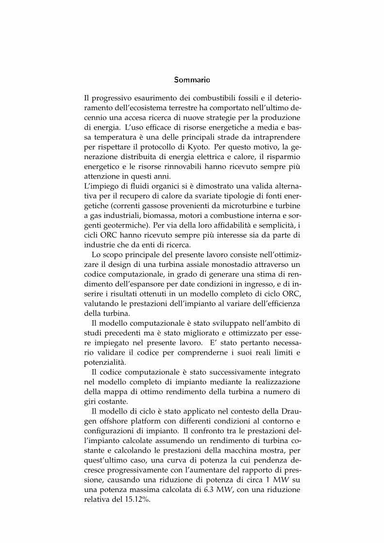
With the shortage of fossil fuel availability and the deteriora-tion of the environment, new strategies and non-conventionalmethodologies for energy supply have been proposed. The ef-fective use of low and medium temperature energy sources isone of the main directions to follow to reduce CO
2emissions
and attend to Kyoto protocol. Distributed electricity (and heat)generation, energy-savings as well as renewable sources thus re-ceived great attention in these last years. The organic Rankinecycle (ORC) technology has proved a valid alternative for wasteheat recovery from different energy sources, e.g. exhausted gasflows from industrial and micro gas turbines, biomass and in-ternal combustion engines. Owing to its feasibility and relia-bility, ORC power systems have received widespread attentionfrom industries and academia.
This work is focused on the optimization of an axial-flow-turbine design by means of a computational model, capableof evaluating turbine efficiency as a function of expander inletconditions, and on the coupling of the obtained results into acomplete ORC power plant model to achieve a more reliableevaluation of its performances.
The computational model had been aforetime developed inthe context of previous studies but it was improved and opti-mized for the purpose of this work. A new validation processin order to verify its performance and reliability was so per-formed.
The turbine code was afterwards integrated with the full cy-cle model. In order to reduce the computational time and en-sure convergence, the turbine efficiency map was built.
The full ORC model was applied in the context of the Drau-ghen offshore platform with different boundary conditions andplant configurations. The comparison between the results ob-tained with a constant-turbine-efficiency model and the onesachieved computing explicitly the expander performance shows,for this latter case, a progressively decrement in turbine effi-ciency for increasing values of pressure ratio, followed by aprogressively flattening power curve.The reduction in output power is almost 1 MW with respect toa maximum estimated power of 6.3 MW, thereby yielding to arelative reduction of about 15.12% in the most general case.
In the next step, the rotational speed was included among theoptimizing parameters and another turbine map was built, al-lowing to evaluate cycle performances accounting for a turbinewith optimized rotational speed. It was found the addition of a

gearbox can significantly improve turbine efficiency, with a ben-efit in power of about 500 kW that implies a relative incrementof 7.5% with respect to the results obtained in the previous case.A first approximated attempt to evaluate the convenience ofa gearbox insertion shows this configuration seems profitable;however, more detailed information about gearbox efficiency,weight and volume, as well as data on the effective load regimeand utilization factor are required to evaluate properly its prof-itability, depending the revenue mainly on this latter parameter.
In the end, a different optimization was performed, aimingto minimize the specific cost instead of maximizing turbine ef-ficiency. The results show the economic-best efficiency configu-ration for the turbine appears to be slightly different from thethermodynamic one, even if the value of obtained specific costand efficiency are very close.
iii
Sommario
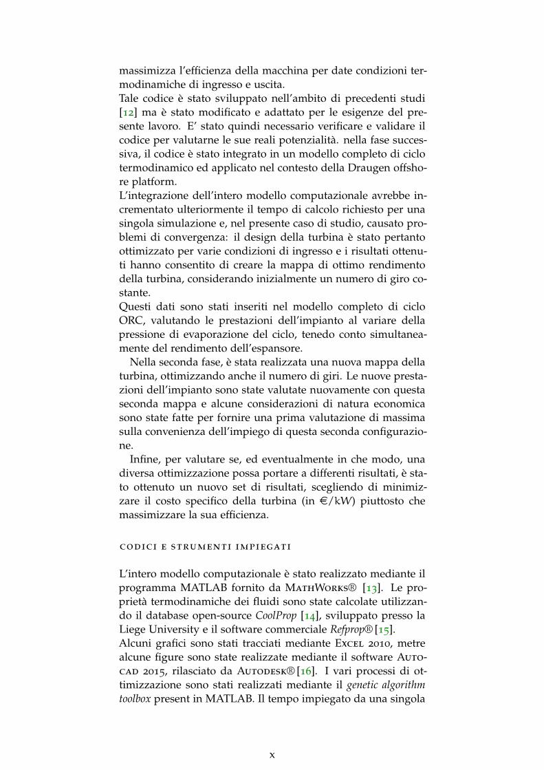
Il progressivo esaurimento dei combustibili fossili e il deterio-ramento dell’ecosistema terrestre ha comportato nell’ultimo de-cennio una accesa ricerca di nuove strategie per la produzionedi energia. L’uso efficace di risorse energetiche a media e bas-sa temperatura è una delle principali strade da intraprendereper rispettare il protocollo di Kyoto. Per questo motivo, la ge-nerazione distribuita di energia elettrica e calore, il risparmioenergetico e le risorse rinnovabili hanno ricevuto sempre piùattenzione in questi anni.L’impiego di fluidi organici si è dimostrato una valida alterna-tiva per il recupero di calore da svariate tipologie di fonti ener-getiche (correnti gassose provenienti da microturbine e turbinea gas industriali, biomassa, motori a combustione interna e sor-genti geotermiche). Per via della loro affidabilità e semplicità, icicli ORC hanno ricevuto sempre più interesse sia da parte diindustrie che da enti di ricerca.
Lo scopo principale del presente lavoro consiste nell’ottimiz-zare il design di una turbina assiale monostadio attraverso uncodice computazionale, in grado di generare una stima di ren-dimento dell’espansore per date condizioni in ingresso, e di in-serire i risultati ottenuti in un modello completo di ciclo ORC,valutando le prestazioni dell’impianto al variare dell’efficienzadella turbina.
Il modello computazionale è stato sviluppato nell’ambito distudi precedenti ma è stato migliorato e ottimizzato per esse-re impiegato nel presente lavoro. E’ stato pertanto necessa-rio validare il codice per comprenderne i suoi reali limiti epotenzialità.
Il codice computazionale è stato successivamente integratonel modello completo di impianto mediante la realizzazionedella mappa di ottimo rendimento della turbina a numero digiri costante.
Il modello di ciclo è stato applicato nel contesto della Drau-gen offshore platform con differenti condizioni al contorno econfigurazioni di impianto. Il confronto tra le prestazioni del-l’impianto calcolate assumendo un rendimento di turbina co-stante e calcolando le prestazioni della macchina mostra, perquest’ultimo caso, una curva di potenza la cui pendenza de-cresce progressivamente con l’aumentare del rapporto di pres-sione, causando una riduzione di potenza di circa 1 MW suuna potenza massima calcolata di 6.3 MW, con una riduzionerelativa del 15.12%.

Nella fase successiva, il numero di giri della macchina è statoottimizzato ed è stata ottenuta una nuova mappa dell’espan-sore, consentendo di calcolare le prestazioni del ciclo con unaturbina a numero di giri ottimizzato. L’incremento di efficien-za dell’espansore consente di aumentare la potenza ottenutadi circa 500 kW, con un incremento relativo di circa il 7.5% ri-spetto ai risultati ottenuti nel test precedente. Una indicazionedi massima sulla convenienza economica legata all’impiego diuna turbina a numero di giri ottimizzato mostra che questa se-conda configurazione sembra essere conveniente. Tuttavia, peruna stima più accurata sono necessari ulteriori dati su peso,volume ed efficienza dello stesso, nonché una stima più accu-rata del fattore di utilizzo e delle effettive condizioni di caricodell’impianto.
Infine, è stato effettuato un ultimo processo di ottimizzazio-ne, scegliendo di minimizzare il costo specifico della turbinaanziché ottimizzare il rendimento. I risultati mostrano che laconfigurazione di minimo costo specifico sono leggermente dif-ferenti da quelle ottenute con una ottimizzazione termodinami-ca, sebbene i valori di efficienza e costo specifico ottenuti neidue processi siano molto vicini.
v

“So long as you still see the stars as something "above you" you stilllack the eye of the man of knowledge.”
Friedrich Nietzsche, Beyond Good and Evil
“Everything should be made as simple as possible, but not simpler.”Albert Einstein

P R E FA Z I O N E
Questo lavoro rappresenta il mio progetto di tesi per la laureamagistrale in ingegneria energetica presso il Politecnico di Mi-lano.L’intero lavoro di tesi è stato svolto presso la Technical Universi-ty of Denmark (DTU). Il presente lavoro corrisponde a 30 CFUed è stato svolto dal 12 maggio 2014 al 5 novembre 2014. Isupervisors sono il Professor Fredrik Haglind e i Ph.D. candi-dates Leonardo Pierobon e Jesper Graa Andreasen dalla DTU eil Professor Giacomo Bruno Persico dal Politecnico di Milano.
Vorrei ringraziare il Professor Haglind per avermi concessol’opportunità di svolgere il mio lavoro di tesi presso questa pre-stigiosa università e il Professor Persico per essere sempre statodisponibile e presente con i suoi consigli, anche se lontano.
Un ringraziamento speciale è dovuto a Leonardo Pierobon eJesper Graa Andreasen per la loro pazienza, i loro consigli e illoro supporto.Questo lavoro avrebbe potuto essere molto dispersivo e il loroconsiglio è stato di aiuto fondamentale per me durante la miapermanenza alla DTU.
vii

P R E FA C E
This present thesis represents my final project for the Master’sdegree in Energy engineering at Politecnico di Milano.The whole study has been carried out at Technical University ofDenmark (DTU), Thermal Energy section. The Master’s thesisconsists in a 30 ECTS project and it was performed by the 12thof May 2014 to the 5th of November 2014.Supervisors were Associate Professor Fredrik Haglind, Ph.D.candidate Leonardo Pierobon, Ph.D. student Jesper Graa An-dreasen from DTU and Ph.D. Giacomo Bruno Persico from Po-litecnico di Milano.I want to thank Professor Fredrik Haglind for giving me thepossibility to perform my final project in this prestigious Uni-versity and Giacomo Bruno Persico for having been alwaysavailable, even far away.
My special thanks and gratitude must be given to LeonardoPierobon and Jesper Graa Andreasen for their patience, theircompetence, their advice and their support.This project could have been very dispersive and their adviceabout which direction to follow have been of fundamental helpfor me during all my period of permanence at DTU.
viii

S I N T E S I D E L L AV O R O D I T E S I
Nel tentativo congiunto di produrre più energia e ridurre leemissioni di biossido di carbonio, i cicli termodinamici alimen-tati da fluidi organici hanno dimostrato di essere un utile stru-mento per raggiungere l’obiettivo.La produzione di potenza da un ciclo termdinamico è stretta-mente lagata alle prestazioni dell’espansore che, a sua volta,variano in funzione dei parametri termodinamici e del fluidoimpiegato.Molti modelli di cicli ORC presenti in letteratura sono realiz-zati assumendo una efficienza della turbina costante: tuttavia,laddove questa ipotesi non è accetabile, le effettive prestazio-ni dell’espansore possono significativamente modificare il realeoutput del ciclo e il suo punto di ottimo da un punto di vistatecnico-economico.
Per ricercare le reali prestazioni di un impianto e trovare ilpunto di ottimo da un punto di vista termodinamico ed econo-mico, è dunque necessario tenere conto dell’effettivo comporta-mento dell’espansore all’interno del ciclo termodinamico.
obiettivi del lavoro
Lo scopo principale del presente lavoro consiste nell’ottimizza-re il design di una turbina assiale monostadio attraverso uncodice computazionale, in grado di generare una stima di ren-dimento dell’espansore per date condizioni in ingresso, e di in-serire i risultati ottenuti in un modello completo di ciclo ORC,valutando le prestazioni dell’impianto al variare della sua pres-sione di evaporazione. Dal confronto con le prestazioni calco-late per il medesimo impianto assumendo un rendimento diturbina costante, sarà possibile stabilire se tale approccio è ingrado di fornire risultati sufficientemente accurati o se un mo-dello più complesso, che tiene conto delle effettive prestazionidell’espansore, risulta invece necessario.
Per lo scopo di questo lavoro, è stato impiegato un modellocomputazionale pre-esistente di turbina: sulla base di un setdi otto parametri di design, portata massica, temperatura diingresso e rapporto di pressione totale tra ingresso e uscita,il codice produce una stima dell’efficienza total-to-total dellamacchina. Qualora inserito in un algoritmo di ottimizzazio-ne, il codice completo può restituire la geometria ottimale che
ix
massimizza l’efficienza della macchina per date condizioni ter-modinamiche di ingresso e uscita.Tale codice è stato sviluppato nell’ambito di precedenti studi[12] ma è stato modificato e adattato per le esigenze del pre-sente lavoro. E’ stato quindi necessario verificare e validare ilcodice per valutarne le sue reali potenzialità. nella fase succes-siva, il codice è stato integrato in un modello completo di ciclotermodinamico ed applicato nel contesto della Draugen offsho-re platform.L’integrazione dell’intero modello computazionale avrebbe in-crementato ulteriormente il tempo di calcolo richiesto per unasingola simulazione e, nel presente caso di studio, causato pro-blemi di convergenza: il design della turbina è stato pertantoottimizzato per varie condizioni di ingresso e i risultati ottenu-ti hanno consentito di creare la mappa di ottimo rendimentodella turbina, considerando inizialmente un numero di giro co-stante.Questi dati sono stati inseriti nel modello completo di cicloORC, valutando le prestazioni dell’impianto al variare dellapressione di evaporazione del ciclo, tenedo conto simultanea-mente del rendimento dell’espansore.
Nella seconda fase, è stata realizzata una nuova mappa dellaturbina, ottimizzando anche il numero di giri. Le nuove presta-zioni dell’impianto sono state valutate nuovamente con questaseconda mappa e alcune considerazioni di natura economicasono state fatte per fornire una prima valutazione di massimasulla convenienza dell’impiego di questa seconda configurazio-ne.
Infine, per valutare se, ed eventualmente in che modo, unadiversa ottimizzazione possa portare a differenti risultati, è sta-to ottenuto un nuovo set di risultati, scegliendo di minimiz-zare il costo specifico della turbina (in e/kW) piuttosto chemassimizzare la sua efficienza.
codici e strumenti impiegati
L’intero modello computazionale è stato realizzato mediante ilprogramma MATLAB fornito da MathWorks® [13]. Le pro-prietà termodinamiche dei fluidi sono state calcolate utilizzan-do il database open-source CoolProp [14], sviluppato presso laLiege University e il software commerciale Refprop® [15].Alcuni grafici sono stati tracciati mediante Excel 2010, metrealcune figure sono state realizzate mediante il software Auto-cad 2015, rilasciato da Autodesk® [16]. I vari processi di ot-timizzazione sono stati realizzati mediante il genetic algorithmtoolbox present in MATLAB. Il tempo impiegato da una singola
x

ottimizzazione può variare da quattro ore a cinque giorni.
metodi e modelli
Introduzione al modello computazionale di turbina
Questo paragrafo fornisce solamente uno sguardo di insiemeal modello computazionale; una descrizione più dettagliata dialcuni aspetti è riportata nella sezione 3.2 a pagina 18, mentreuna trattazione completa ed esaustiva dell’argomento è fornitada Gabrielli [12].
L’intero algoritmo di design della turbina è basato su un set diotto parametri i cui valori, insieme alle condizioni di ingresso euscita della macchina, consentono di pervenire ad una stima fi-nale del rendimento. Tali parametri, insieme alle condizioni ter-modinamiche in ingresso e uscita della macchina, sono elencatinella tabella 3.2 a pagina 19. Come riportato, è necessario forni-re atri valori oltre a quelli già menzionati, come ad esempio larugosità superficiale. Tuttavia, questi valori sono scelti per mas-simizzare l’efficienza compatibilmente con le attuali possibilitàtecnologiche e sono tenuti costanti durante l’intero processo diottimizzazione. Una lista completa di tutti i parametri richiestidal codice è riportata in tabella B.1 a pagina 95 in appendice B.Per un certo set di valori per i parametri di input riportati intabella 3.2, il codice restituisce quindi un valore di efficienzatotal-to-total della macchina, assumendo una componente as-siale di velocità costante per tutto lo stadio.Si noti che questa configurazione non è l’unica possibile, maper una geometria che non consideri una componente assialedi velocità constante lungo lo stadio, sono necessari altri dueparametri di input, ossia la componente assiale di velocità iningresso Ca1 e il coefficiente φr, definito nella equazione 3.2 apagina 20. questa variante è stata adottata durante la fase diverifica e validazione del codice.Si noti infine che:
• la valutazione delle perdite è effettuata con il modello diCraig e Cox [4] che risulta essere, secondo precedenti stu-di, il più completo e adatto allo scopo di questo lavoro[22, 23, 27, 28];
• nella geometria creata dal codice (riportata in figura 3.4 apagina 21), la forma delle pale rotoriche è sempre conver-gente, mentre quella delle pale statoriche può cambiareda convergente a convergente-divergente;
xi
• il codice assume flusso monodimensionale e non tieneconto di alcuna variazione in direzione radiale del pro-filo di velocità nè considera un eventuale svergolamentodelle pale.
La struttura principale del modello computazionale è essen-zialmente composta da tre parti:
1. Valutazione di tutte le variabili termodinamiche in ingres-so e proprietà isoentropiche in uscita. Questo passaggioconsente di calcolare il salto entalpico totale isoentropi-co. Tutti questi valori restano costanti durante le fasisuccessive del processo;
2. Ottenimento di un set di valori di primo tentativo perangoli di flusso, velocità e proprietà termodinamiche delfluido in tutto lo stadio;
3. Ciclo iterativo: iniziando dai valori di primo tentativo ap-pena ottenuti, viene avviato un processo iterativo finchéla convergenza non viene raggiunta.
Se, come precedentemente accennato, questo modello è ac-coppiato con un opportuno algoritmo di ottimizzazione, perun dato fluido e date condizioni termodinamiche in ingresso1, èpossibile pervenire al set ottimale di parametri che massimizzal’efficienza della macchina. L’algoritmo impiegato è chiamatoalgoritmo genetico, integrato di default nella optimization tool-box del programma MATLAB e la sua logica di funzionamentoè brevemente descritta in appendice A a pagina 91.
Per ottenere soluzioni accettabili sia da un punto di vista fisicoche tecnologico, è necessario imporre alcuni vincoli geometricie termodinamici, che si concretizzano in:
• un limite superiore e inferiore per ognuno dei parame-tri da ottimizzare (richiesto peraltro dall’algoritmo di otti-mizzazione);
• un secondo set di vincoli ulteriormente imposto sulla so-luzione finale.
Tali vincoli sono stati sostanzialmente stabiliti da Macchi ePerdichizzi [27] e sono riportati nelle tabelle 3.3 e 3.4 a pagi-na 24.Come meglio discusso nel paragrafo 3.3.4 a pagina 24, l’impo-sizione dei vincoli si basa sostanzialmente su tre ragioni:
1 Portata massica, rapporto di pressione totale tra ingresso e uscita della mac-china, temperatura totale in ingresso, numero di giri (quest’ultimo saràinvece inserito tra i parametri di ottimizzare nella seconda parte del lavoro).
xii

• alcuni sono necessari per assicurare la validità delle corre-lazioni usate e la compatibilità con la geometria generatadal modello;
• altri sono imposti per ragioni di tipo tecnologico;
• alti ancora sono imposti per contenere l’insorgere di effet-ti radiali e tridimensionali, di cui il codice, come primamenzionato, non tiene conto.
Caso di studio: la Draugen offshore platform
La Draugen offshore platform si trova nel mar del Nord, a circa150 km da Kristiansund in Norvegia, distante 200 km dal circo-lo polare artico.Svariate compagnie petrolifere possiedono una quota della piat-taforma, come Shell, Petoro e BP Norge. La piattaforma estraepetrolio e gas naturale che trasporta in Norvegia mediante laAsgard transport pipeline. Maggiori informazioni sono forniteda Offshore Technology [11] ma alcune di esse sono riportatenella sezione 3.1 a pagina 16.L’energia necessaria alla piattaforma (carico normale e di picco)è prodotta mediante tre turbine a gas Siemens SGT-500. Si trat-ta di macchine in grado di produrre potenza tra i 15 e 20 MW.Le specifiche techiche della macchina sono fornite da Siemens[5] e sono riportate in tabella 3.1 a pagina 18.Nella piattaforma, una di queste turbine rimane spenta e in ma-nutenzione, mentre le altre due forniscono l’energia richiesta.Nel presenta lavoro verrà esaminata soltanto una turbina a gas,senza considerare il resto dell’impianto presente nella piattafor-ma. Soltanto in un caso anche la seconda turbina a gas verràconsiderata nello schema di impianto.Si assume di alimentare la macchina mediante gas naturale ma,poichè la turbina Siemens SGT-500 può essere alimentata conuna vasta gamma di combustibili, la temperatura minima discarico dei gas dalla waste heat recovery unit è prudentemen-te fissata a 145 ◦C per evitare la formazione di condense acide[29].Secondo Pierobon et al. [7], la installazione di una unità ORCdi recupero di calore dai gas di scarico, comporterebbe due fon-ti di guadagno: la prima, legata al risparmio sul combustibile,che potrebbe essere pertanto esportato dalla piattaforma e ven-duto; la seconda, legata alla riduzione delle emissioni di CO
2
legata alla combustione del gas naturale: dal 1991, infatti, il go-verno norvegese impone una carbon tax sulle emissioni di CO
2
da cobustibili fossili [30]; l’unità installata ridurrebbe quindi
xiii

l’ammontare della tassa per via della “mancata” combustionedel gas naturale risparmiato.
Modello di impianto
Lo schema di impianto del modello impiegato è riportato infigura 3.15 a pagina 33. Il modello di ciclo è stato realizzatoassumendo le seguenti ipotesi:
• Sono considerate solo configurazioni subcritiche (la mas-sima pressione possibile è fissata a 0.9 · Pcr)
• Non sono considerate perdite di carico all’interno dell’im-pianto;
• La corrente di gas di scarico della turbina a gas è assuntacome ideale;
• La localizzazione del ∆Tpp nello scambiatore di calore prin-cipale può spostarsi dall’ingresso dell’evaporatore all’u-scita del rigeneratore, qualora necessario (si veda la figu-ra 3.16 a pagina 35);
Per ridurre il numero di parametri di impianto da ottimizzare,sono state fatte inoltre le seguenti assunzioni:
1. Il ciclopentano è stato scelto come fluido di lavoro risul-tando, secondo Pierobon et al. [7], la scelta ottimale per ilcaso in esame;
2. Entrambe le differenze di temperatura di pinch point, ∆Tppe ∆Tpp,rec, sono state fissate al minimo (e ottimo) valoreriportato da Pierobon et al. [7], rispettivamente 10 e 15 ◦C;
3. La pressione di condensazione è stata fissata a 1 bar perevitare infiltrazioni di aria che comporterebbero la rapidadecomposizione del fluido [21];
4. La temperatura di ingresso in turbina è stata fissata almassimo valore che assicura la integrità chimica del flui-do evitandone la decomposizione; tale valore risulta esse-re 513.15 K [21].
Per quanto appena discusso, entrambe le mappe della turbi-na sono state ottenute per il ciclopentano2 considerando unatemperatura di ingresso in turbina costante e pari a 513.15 K.Le mappe riportano i valori di efficienza ottenuta in funzionedella portata massica e vari valori del rapporto di pressione esono integrate nel modello di ciclo mediante una funzione la
2 la cui pressione critica è 45.71 bar.
xiv

cui sintassi è fornita dalla equazione 3.9 a pagina 32. Si notiche il punto di scarico della turbina influenza la quantità dicalore recuperabile dal fluido dopo l’espansione e dunque, ilpunto di uscita dal rigeneratore. Qualora la localizzazione del∆Tpp sia all’uscita del rigeneratore, questo punto influenza laportata massica di fluido di lavoro attraverso il bilancio ener-getico dello scambiatore di calore gas-fluido e dunque, infine,il rendimento della turbina. Risulta necessario in questo casoun processo iterativo, la cui convergenza, nel caso in cui l’inte-ro modello computazionale dell’espansore fosse direttamenteintegrato nel ciclo, risulterebbe estremamente lenta se non im-possibile nella maggior parte dei casi, in quanto le fluttuazionidi portata massica presenti durante le iterazioni non potrebbe-ro essere seguite da una simultanea variazione del design dellamacchina, con un conseguente valore nullo di efficienza mo-strato dal codice. L’impiego della mappa della turbina risultapertanto necessario per ottenere la convergenza nel processoiterativo.Una lista completa di tutti gli input richiesti dal modello diciclo è riportata in tabella B.2 a pagina 96.
Stima di massima sulla convenienza dell’impiego di un gearbox
L’ottimizzazione del numero di giri della macchina consente diottenere una geometria differente con una efficienza più alta,ma comporta anche l’impiego di un riduttore/moltiplicatore digiri. Una stima accurata del profitto economico legato al suoimpiego richiederebbe il calcolo del valore attuale netto (VAN)per le due configurazioni di impianto e il loro confronto, com-portando pertanto un esame del costo di tutti i componenti del-l’impianto. Tale indagine è al di là degli scopi del presentelavoro ma, per ottenere una prima stima di massima sulla even-tuale convenienza di impiego una turbina con numero di giriottimizzato, è sufficiente calcolare il valore attuale netto per unimpianto con e senza riduttore, preoccupandosi solo del costodella macchina, generatore elettrico e riduttore e sottrarre i duevalori. Infatti, le dimensioni (e il costo) di uno scambiatore dicalore sono in prima approssimazione legati alla portata massi-ca che circola e al livello di pressione. Pertanto, per dato rap-porto di pressione, è possibile considerare le dimensioni degliscambiatori approssimativamente costanti per i due casi, tenen-do a mente anche che, come sarà successivamente discusso, lavariazione del rendimento della turbina non cambia significati-vamente la portata di fluido di lavoro che circola nell’impianto.Il costo della turbina, generatore e riduttore/moltiplicatore digiri è stato stimato mediante le funzioni di costo adoperate da
xv
Astolfi et al. [20], riportate a pagina 38 e 41, mentre i ricavidell’impianto legati, come già discusso, alla vendita del combu-stibile risparmiato e alla riduzione della carbon tax sono statiottenuti mediante la metodologia impiegata da Pierobon et al.[7] e riportata nel paragrafo 3.9 a pagina 39.
Infine, per l’ultimo processo di ottimizzazione, il costo spe-cifico della turbina è stato ricavato impiegando nuovamente lafunzione di costo fornita dalla espressione 3.18 a pagina 38 escegliendo questo parametro come la funzione da minimizzare.
verifica e validazione del codice
Le prestazioni del modello computazionale di turbina sono sta-te mediante due processi:
1. Una verifica con il codice AXTUR;
2. Una validazione con un set di dati sperimentali ottenutida Evers and Kötzing [6].
Verifica con AXTUR
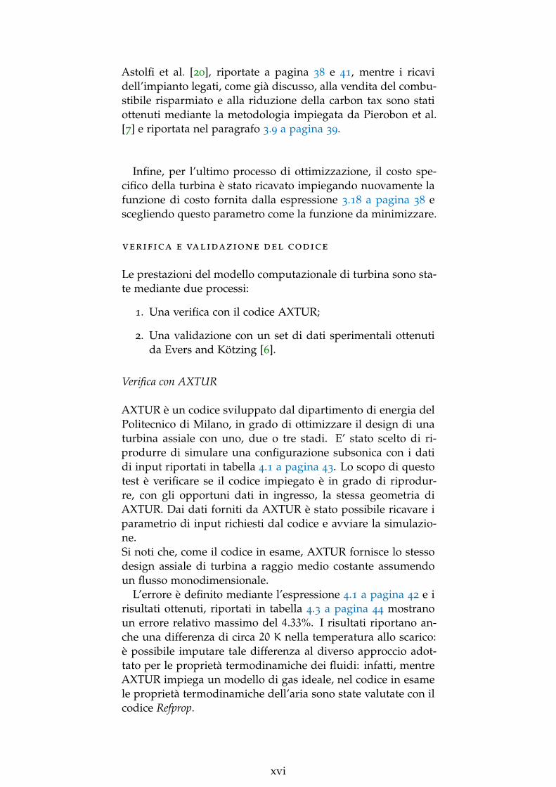
AXTUR è un codice sviluppato dal dipartimento di energia delPolitecnico di Milano, in grado di ottimizzare il design di unaturbina assiale con uno, due o tre stadi. E’ stato scelto di ri-produrre di simulare una configurazione subsonica con i datidi input riportati in tabella 4.1 a pagina 43. Lo scopo di questotest è verificare se il codice impiegato è in grado di riprodur-re, con gli opportuni dati in ingresso, la stessa geometria diAXTUR. Dai dati forniti da AXTUR è stato possibile ricavare iparametrio di input richiesti dal codice e avviare la simulazio-ne.Si noti che, come il codice in esame, AXTUR fornisce lo stessodesign assiale di turbina a raggio medio costante assumendoun flusso monodimensionale.
L’errore è definito mediante l’espressione 4.1 a pagina 42 e irisultati ottenuti, riportati in tabella 4.3 a pagina 44 mostranoun errore relativo massimo del 4.33%. I risultati riportano an-che una differenza di circa 20 K nella temperatura allo scarico:è possibile imputare tale differenza al diverso approccio adot-tato per le proprietà termodinamiche dei fluidi: infatti, mentreAXTUR impiega un modello di gas ideale, nel codice in esamele proprietà termodinamiche dell’aria sono state valutate con ilcodice Refprop.
xvi

Validazione con Evers e Kötzing
Evers e Kötzing riportano i dati di una turbina assiale a quattrostadi alimentata ad aria. La geometria è riportata in figura 4.2,mentre i dati adoperati e immagini relative alla geometria dellepale sono riportati in appendice C.
All’ingresso di ogni stadio e all’uscita dell’ultimo, le proprie-tà termodinamiche del fluido sono state fornite in nove puntilungo l’altezza di pala. Questi dati, insieme alle informazio-ni sulla geometria delle pale, consentono di ricavare il set diparametri di input necessari al codice. Tutti i valori di input im-piegati sono stati estrapolati per mezzo dei dati forniti al raggiomedio del particolare stadio. E’ stato scelto di validare il codicesolo con i dati del primo e ultimo stadio.
I risultati ottenuti per il primo stadio, riportati in tabella 4.6a pagina 48, mostrano un errore relativo massimo del 22.38%rispetto l’altezza di pala. Tale errore è principalmente imputa-bile alla non-rappresentatività del valore adoperato di velocitàassiale al raggio medio in termini di portata massica: infatti, l’a-rea di passaggio del fluido e, successivamente, l’altezza di pala,sono valutate per mezzo delle equazioni 4.2 e 4.5 a pagina 50;pertanto, per data portata massica e raggio medio, un eventua-le “eccesso” legato alla velocità assiale deve essere compensatoda una proporzionale riduzione di altezza di pala.
I risultati ottenuti per l’ultimo stadio, riportati in tabella 4.7 apagina 49, mostrano la stessa tipologia di errore con valori piùalti, dovuti alla variazione ancora più marcata del profilo assia-le di velocità in direzione radiale, come riportato dai grafici infigura 4.4 e 4.5.
Infine, il grafico in figura 4.3 a pagina 51 mostra la elevatasensibilità dell’angolo di uscita α3 rispetto all’angolo β3: risultadunque possibile comprendere come una piccola incertezza suquest’ultimo angolo risulti in una amplificazione di circa trevolte nell’errore relativo all’angolo α3, riscontrata nei risultatiper entrambi gli stadi.
discussione dei risultati
I risultati ottenuti si possono dividere in tre gruppi:
1. Risultati riguardanti l’ottimizzazione del design della tur-bina, raggruppati nelle due mappe di funzionamento del-la macchina;
2. Risultati riguardanti le prestazioni del ciclo termodinami-co;
xvii

3. Risultati riguardanti la ottimizzazione tecnico-economicadella turbina.
Mappe della turbina
I valori di massimo rendimento ottenuti ottimizzando il designdella turbina con numero di giri fisso a 3000 rpm sono riportatinella prima mappa della macchina (figura 5.1 a pagina 54), chemostra l’efficienza in funzione di portata massica e rapportodi pressione. Il rendimento cresce all’aumentare della portatamassica e diminuisce all’aumentare del rapporto di pressione.Come meglio discusso nella sezione 5.1, alcuni valori limite im-posti dai vincoli sono raggiunti durante il processo di ottimiz-zazione, ossia il valore massimo del numero di Mach MW3 espesso il valore minimo di (o/s)n e il numero massimo di palestatoriche.
L’inserimento del numero di giri tra i parametri da ottimiz-zare consente di avere un grado di libertà in più, che comportala possibilità di raggiungere efficienze più alte, specialmentenell’intervallo di portata tra 20 e 80 kg/s, ossia l’intervallo diportata massica in cui il numero di giri ottimo risulta marca-tamente differente da 3000 rpm (si vedano le figure 5.7 e 5.8a pagina 58). In questo caso i vincoli più stringenti risultanoessere l’angolo di flare del rotore e nuovamente, il numero diMach MW3.
Prestazioni dell’impianto
Le prestazioni dell’impianto sono state riportate in grafici chemostrano la curva di potenza in funzione del rapporto di pres-sione tra ingresso e uscita della macchina ossia, per la ipotiz-zata assenza di perdite di carico, tra pressione di evaporazionee pressione di condensazione. Infatti, per le assunzioni fatteprecedentemente, questo parametro risulta l’unico in grado diinfluenzare le prestazioni dell’impianto. L’intervallo operativodi rapporto di pressione varia da 1 a 41. Per facilitare il con-fronto, le curve di potenza ottenute calcolando le prestazionidell’espansore sono state affiancate alle curve di potenza di unimpianto in cui è stata assunta un’efficienza di turbina costante.Per la prima parte dei risultati è stata impiegata solo la mappadella turbina a numero di giri costante; la seconda mappa è sta-ta invece impiegata nella fase successiva.
xviii
Test con numero di giri fisso
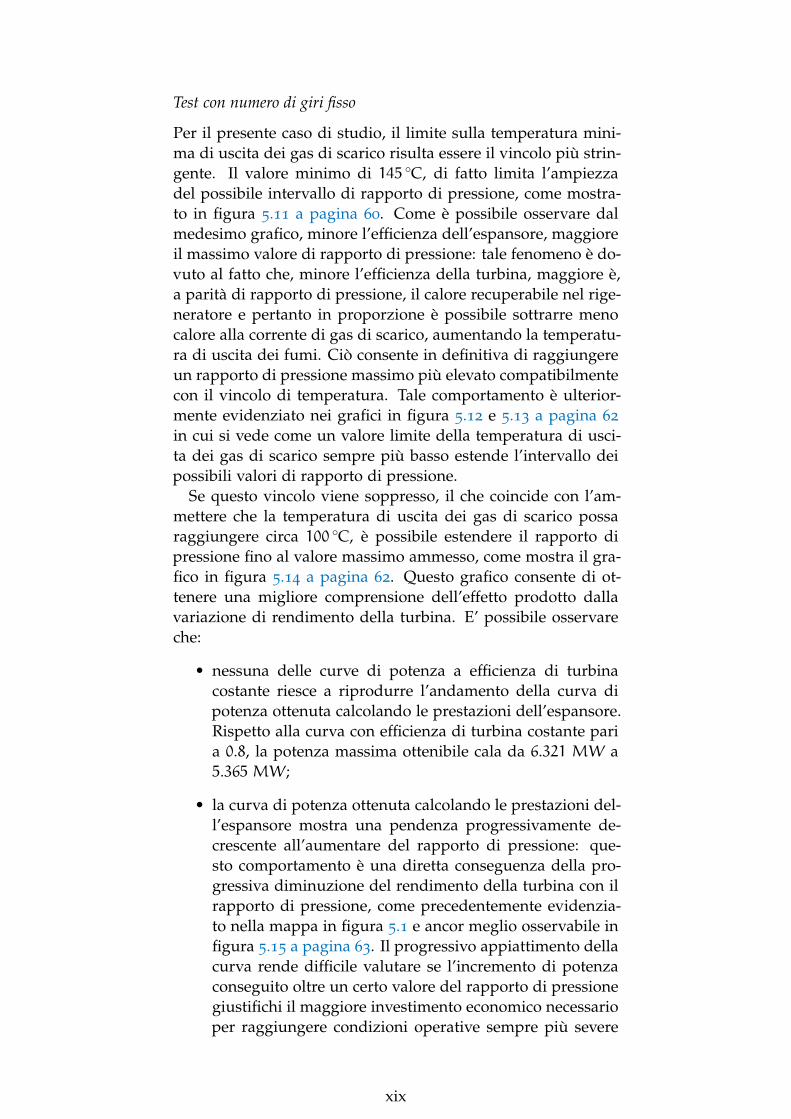
Per il presente caso di studio, il limite sulla temperatura mini-ma di uscita dei gas di scarico risulta essere il vincolo più strin-gente. Il valore minimo di 145 ◦C, di fatto limita l’ampiezzadel possibile intervallo di rapporto di pressione, come mostra-to in figura 5.11 a pagina 60. Come è possibile osservare dalmedesimo grafico, minore l’efficienza dell’espansore, maggioreil massimo valore di rapporto di pressione: tale fenomeno è do-vuto al fatto che, minore l’efficienza della turbina, maggiore è,a parità di rapporto di pressione, il calore recuperabile nel rige-neratore e pertanto in proporzione è possibile sottrarre menocalore alla corrente di gas di scarico, aumentando la temperatu-ra di uscita dei fumi. Ciò consente in definitiva di raggiungereun rapporto di pressione massimo più elevato compatibilmentecon il vincolo di temperatura. Tale comportamento è ulterior-mente evidenziato nei grafici in figura 5.12 e 5.13 a pagina 62
in cui si vede come un valore limite della temperatura di usci-ta dei gas di scarico sempre più basso estende l’intervallo deipossibili valori di rapporto di pressione.
Se questo vincolo viene soppresso, il che coincide con l’am-mettere che la temperatura di uscita dei gas di scarico possaraggiungere circa 100 ◦C, è possibile estendere il rapporto dipressione fino al valore massimo ammesso, come mostra il gra-fico in figura 5.14 a pagina 62. Questo grafico consente di ot-tenere una migliore comprensione dell’effetto prodotto dallavariazione di rendimento della turbina. E’ possibile osservareche:
• nessuna delle curve di potenza a efficienza di turbinacostante riesce a riprodurre l’andamento della curva dipotenza ottenuta calcolando le prestazioni dell’espansore.Rispetto alla curva con efficienza di turbina costante paria 0.8, la potenza massima ottenibile cala da 6.321 MW a5.365 MW;
• la curva di potenza ottenuta calcolando le prestazioni del-l’espansore mostra una pendenza progressivamente de-crescente all’aumentare del rapporto di pressione: que-sto comportamento è una diretta conseguenza della pro-gressiva diminuzione del rendimento della turbina con ilrapporto di pressione, come precedentemente evidenzia-to nella mappa in figura 5.1 e ancor meglio osservabile infigura 5.15 a pagina 63. Il progressivo appiattimento dellacurva rende difficile valutare se l’incremento di potenzaconseguito oltre un certo valore del rapporto di pressionegiustifichi il maggiore investimento economico necessarioper raggiungere condizioni operative sempre più severe
xix

e mostra come sia necessario tenere conto delle effettiveprestazioni della turbina per indagini successive.
Un secondo test effettuato considera lo sfruttamento di en-trambe le turbine a gas presenti nella piattaforma. Lo scopo diquesto test è duplice:
• Consente di valutare le prestazioni della turbina in uncampo diverso da quello precedente, modificando il rangedi valori di portata massica nell’impianto;
• Consente di valutare l’eventuale beneficio di installare unaunica unità di recupero più grande che sfrutti entrambi iflussi di gas di scarico rispetto a due unità identiche sepa-rate; il nuovo schema di impianto è riportato in figura 5.21
a pagina 68.
Il grafico delle curve di potenza ottenute, riportato in figu-ra 5.25 a pagina 71, mostra un comportamento analogo a quel-lo precedente, pur tuttavia con una importante differenza: ilvalore doppio di portata di gas di scarico implica una portatacirca doppia di fluido nel ciclo sottoposto, con un proporzio-nale incremento della potenza in uscita; tuttavia, mentre perun modello ad efficienza di turbina costante un valore doppiodi portata di fluido corrisponde esattamente ad un valore dop-pio di potenza prodotta, nel caso in cui vengano calcolate leprestazioni della macchina si ha un valore di potenza più cheraddoppiato, dovuto al proporzionale miglioramento della ef-ficienza della stessa (si confrontino le figure 5.15 a pagina 63
e 5.26 a pagina 72). Per la massima potenza prodotta di ha unincremento relativo del 6.24%.
Test con numero di giri ottimizzato
L’ottimizzazione del numero di giri, e dunque l’impiego dellaseconda mappa della turbina, consente di incrementare il ren-dimento dell’espansore di quasi il 10%, come riportato in figu-ra 5.28 a pagina 73, con un conseguente incremento massimodi potenza di quasi 500 kW3 (si veda la successiva figura 5.29).
Il grafico di figura 5.30 mostra le curva di potenza ottenu-ta per tre diversi valori di efficienza di trasmissione meccanica:è possibile osservare come un rendimento inferiore a al 94%sostanzialmente annulli il beneficio dato dalla maggiore com-plessità impiantistica e il conseguente maggiore investimentoeconomico. Normalmente i rendimenti di trasmissione mecca-nica sono superiori al 96%, tuttavia questo grafico mostra come
3 Per il tracciamento dei grafici è stato utilizzato un rendimento ditrasmissione meccanica pari a 0.96.
xx

la maggiore complessità impiantistica sia giustificata solo se ta-le efficienza è superiore ad un valore minimo. Si noti infine chela quantità di informazioni disponibili in letteratura su sistemidi trasmissione meccanica per potenze di ordini di grandez-za pari o superiori a quelle in esame risulta piuttosto contenu-ta, in quanto tali componenti sono solitamente realizzati sottospecifica commissione per il particolare caso.
Una prima stima di massima sulla convenienza dell’impie-go di una turbina a numero di giri ottimizzato è ottenuta co-me differenza di valore attuale netto tra due configurazioni diimpianto, rispettivamente con e senza riduttore. I risultati, ri-portati nel grafico in figura 5.31 a pagina 78 per due fattori diutilizzo, mostrano come questa configurazione sembri essereconveniente, purché il rapporto di pressione sia superiore a 15.E’ interessante notare come il massimo beneficio netto ottenu-to risulti pari circa al 5% del valore attuale netto ottenuto neiprecedenti studi effettuati da Pierobon et al. [7]. Tuttavia, unaanalisi più dettagliata e maggiori informazioni sono necessarieper valutare la effettiva convenienza di questa configurazione,soprattutto riguardo l’effettivo fattore di utilizzo dell’impiantononché peso e volume dei vari componenti, essendo questi dueparametri un vincolo importante in una piattaforma offshore.
Ottimizzazione tecnico-economica della turbina
I risultati ottenuti sono riportati nella sezione 5.4, illustrando lecurve di costo specifico, efficienza e rapporto di portate volume-triche tra uscita e ingresso della macchina per le ottimizzazionieffettuate minimizzando il costo specifico, insieme agli analo-ghi risultati ottenuti precedentemente ricercando la massimaefficienza della macchina.
Come è possibile notare dal grafico in figura 5.33, i risultatisono abbastanza simili anche se non identici. Per ogni simula-zione, il costo specifico risulta sempre minore nel caso della ot-timizzazione tecnico-economica, così come il rendimento dellaturbina risulta sempre maggiore nel caso della ottimizzazione“tradizionale” (figura 5.34).Da un punto di vista teorico, massimizzare l’efficienza coincidecon l’aumento della massima potenza estraibile dalla macchinaper date condizioni di ingresso e uscita e dunque, questo com-porterebbe la minimizzazione del costo specifico. Tuttavia, ilcosto di una turbomacchina è più legato al suo volume che al-la sua efficienza; una informazione utile sulle dimensioni dellamacchina è fornita dal size parameter, definito dalla equazio-ne 3.19 a pagina 38 e presente nella funzione di costo impiega-ta (equazione 3.18). Minimizzare il costo coincide quindi con
xxi

la riduzione del size parameter, che per dato rapporto di pres-sione è funzione solo della portata volumetrica in uscita. Unariduzione di questa ultima coincide con una densità più altaallo scarico e quindi con una minore espansione e comporta,infine, una minore efficienza. Dunque la ricerca della massi-ma efficienza e la riduzione del size parameter non sono duepercorsi indipendenti tra loro. I risultati ottenuti mostrano chevi è un certo intervallo di valori di size parameter in cui la ri-duzione di quest’ultimo ha un effetto benefico sulla riduzionedel costo specifico, nonostante la corrispondente diminuzionedi efficienza. Tuttavia, tale intervallo di valori, sia in termini disize parameter che di efficienza e costo specifico, risulta moltocontenuto, per cui non appare possibile stabilire se l’approccioseguito possa portare a conclusioni apprezzabilmente differentirispetto a quanto precedentemente ottenuto.
conclusioni
Un modello computazionale pre-esistente di turbina, in gradodi stimare il rendimento di una macchina assiale monostadio,è stato ottimizzato e adattato alle esigenze e gli scopi del pre-sente lavoro. Nella fase di verifica e validazione, il codice hariportato apprezzabile accordo con un modello computaziona-le precedentemente sviluppato, ma ha mostrato anche dei limitidi affidabilità qualora siano presenti forti variazioni radiali delprofilo di velocità. Per contenere il problema e assicurare la at-tendibilità dei risultati da un punto di vista fisico e tecnologico,svariati vincoli sono stati imposti restringendo il possibile cam-po di soluzioni accettabili.
I valori di massimo rendimento ottenuti dal processo di otti-mizzazione hanno consentito di tracciare due mappe di efficien-za della turbina, che sono state successivamente integrate inun modello completo di ciclo ORC applicato nel contesto dellaDraugen offshore platform. L’efficienza dell’espansore aumen-ta all’aumentare della portata massica e diminuisce per valoricrescenti del rapporto di pressione.
Il confronto tra le prestazioni dell’impianto ottenute assumen-do un’efficienza di turbina costante e calcolando le prestazionidell’espansore mostra una curva di potenza con pendenza pro-gressivamente decrescente all’aumentare del rapporto di pres-sione, dovuta alla progressiva diminuzione del rendimento del-la turbina. Ciò complica la individuazione dell’effettivo puntodi ottimo da un punto di vista tecnico-economico e mostra co-me sia necessario considerare l’effettivo comportamento della
xxii

macchina per indagini future.
Un successivo test effettuato raddoppiando la portata di gasdi scarico, mostra una potenza prodotta più che raddoppiata,dovuta ad un incremento di efficienza della turbina per valoricrescenti di portata massica.
L’ottimizzazione del numero di giri della macchina consentedi ottenere un beneficio in termini di efficienza di circa il 10%,a cui può corrisponde un incremento di potenza di quasi 500kW. L’impiego di una turbina a numero di giri ottimizzatocomporta comunque un costo aggiuntivo dovuto al sistema ditrasmissione meccanica, nonché un maggiore peso e volumecomplessivo. Una prima stima di massima ottenuta come dif-ferenza del valore attuale netto delle due configurazioni im-piantistiche riporta che questa seconda configurazione sembraessere conveniente, sebbene indagini e informazioni più detta-gliate, soprattutto sull’effettivo fattore di utilizzo e regime dicarico dell’impianto, siano necessarie per stimarne la effettivaconvenienza nel caso in esame, in cui peraltro peso e volumedei componenti hanno un ruolo non trascurabile.
Infine, un diverso processo di ottimizzazione del design del-la turbina, scegliendo di minimizzare il costo specifico anzichémassimizzare l’efficienza, non mostra una apprezzabile diffe-renza nei risultati finali rispetto alle precedenti ottimizzazioni:sebbene infatti per dato rapporto di pressione vi sia un cer-to intervallo di valori in cui una riduzione dell’efficienza dellamacchina ha un effetto benefico sul costo specifico nonostantela riduzione di potenza, tale intervallo di valori, sia in terminidi costo specifico che di efficienza, risulta estremamente conte-nuto e sembra che questo approccio non consenta di ottenererisultati apprezzabilmente diversi dai precedenti.
xxiii

C O N T E N T S
1 introduction 1
1.1 Aims of the work . . . . . . . . . . . . . . . . . . . 1
1.2 Computational tools . . . . . . . . . . . . . . . . . 2
1.3 Structure of the work . . . . . . . . . . . . . . . . . 2
2 background 4
2.1 General overview of of organic Rankine cycles . . 4
2.2 Working fluid selection and cycle set-up . . . . . . 5
2.3 Turboexpanders for organic Rankine cycles . . . . 7
2.3.1 Turbine efficiency . . . . . . . . . . . . . . . 8
2.3.2 Velocity triangles . . . . . . . . . . . . . . . 9
2.3.3 Eulerian work . . . . . . . . . . . . . . . . . 11
2.3.4 Degree of reaction . . . . . . . . . . . . . . 11
2.3.5 Mach number . . . . . . . . . . . . . . . . . 12
2.3.6 Turbine losses . . . . . . . . . . . . . . . . . 13
3 methodology 16
3.1 Case of study: the Draugen offshore platform . . 16
3.2 General overview of turbine design code . . . . . 18
3.3 Code description . . . . . . . . . . . . . . . . . . . 20
3.3.1 First guess values calculation . . . . . . . . 22
3.3.2 Iterative loop . . . . . . . . . . . . . . . . . 22
3.3.3 Optimization process . . . . . . . . . . . . . 23
3.3.4 Constraints on the solution . . . . . . . . . 24
3.4 Influence analysis of optimizing variables . . . . . 25
3.4.1 stage load coefficient ψ and absolute tur-bine inlet angle α1 . . . . . . . . . . . . . . 26
3.4.2 Throat section/pitch ratio for stator androtor (o/s)n and (o/s)r . . . . . . . . . . . . 28
3.4.3 Throat sections (omin)n, or and axial chordscn, cr . . . . . . . . . . . . . . . . . . . . . . 30
3.5 Turbine map . . . . . . . . . . . . . . . . . . . . . . 31
3.6 Cycle model . . . . . . . . . . . . . . . . . . . . . . 32
3.6.1 Fluid properties . . . . . . . . . . . . . . . . 35
3.6.2 ORC model description . . . . . . . . . . . 35
3.7 Optimization accounting for rotational speed . . . 38
3.8 Turbine techno-economic optimization . . . . . . . 38
3.9 Estimation of gearbox profitability . . . . . . . . . 39
4 verification and validation of the code 42
4.1 Verification with AXTUR code . . . . . . . . . . . 42
4.2 Validation with Evers and Kötzing . . . . . . . . . 45
xxiv
4.2.1 Discussion of Results . . . . . . . . . . . . . 50
4.3 Conclusions . . . . . . . . . . . . . . . . . . . . . . 53
5 discussion of results 54
5.1 Turbine maps . . . . . . . . . . . . . . . . . . . . . 54
5.1.1 Map for constant rotational speed . . . . . 54
5.1.2 Turbine map for optimized rotational speed 57
5.2 Cycle tests . . . . . . . . . . . . . . . . . . . . . . . 60
5.2.1 Test with double exhausted gas mass flowrate . . . . . . . . . . . . . . . . . . . . . . . 67
5.3 Tests with optimized rotational speed . . . . . . . 73
5.4 Turbine techno-economic optimization . . . . . . . 79
5.5 Discussion of uncertainties . . . . . . . . . . . . . . 81
6 conclusions and possible future work 83
6.0.1 Future work . . . . . . . . . . . . . . . . . . 85
Bibliography 87
a the genetic algorithm 91
b tables and useful figures 94
c data and pictures from evers and kötzing 98
xxv

L I S T O F TA B L E S
Table 2.1 List of turbine losses according to Craigand Cox method, Craig and Cox [4]. . . . 14
Table 3.1 Design point specifications for SiemensSGT-500 [5] . . . . . . . . . . . . . . . . . . 18
Table 3.2 List of Turbine input parameters and bound-ary conditions . . . . . . . . . . . . . . . . 19
Table 3.3 List of upper and lower bound for thenine turbine design parameters to be op-timized. . . . . . . . . . . . . . . . . . . . . 24
Table 3.4 Other constraints on turbine geometry. . . 24
Table 3.5 Parameter assumed for the economic anal-ysis . . . . . . . . . . . . . . . . . . . . . . 40
Table 4.1 Provided input data for AXTUR . . . . . . 43
Table 4.2 Input data provided for turbine code. . . 43
Table 4.3 Comparison between the results showedby AXTUR and the ones obtained by thecode. . . . . . . . . . . . . . . . . . . . . . . 44
Table 4.4 Turbine design data, Evers and Kötzing [6] 46
Table 4.5 Final set of input values to test the codefor first and fourth stage. . . . . . . . . . . 47
Table 4.6 Results of validation test for stage I. . . . 48
Table 4.7 Results of validation test for stage IV . . . 49
Table 5.1 Cycle parameters for the two maximum-power configurations, with constant andcomputed turbine efficiency. . . . . . . . . 65
Table 5.2 Cycle parameters for the two maximum-power configurations with a double valueof exhausted gas mass flow rate, for con-stant and computed turbine efficiency. . . 70
Table 5.3 Results of net present value differencefor the three examined configurations andhu = 7000. . . . . . . . . . . . . . . . . . . 76
Table 5.4 Results of net present value differencefor the three examined configurations andhu = 4380. . . . . . . . . . . . . . . . . . . 77
Table 5.5 Estimated total investment cost and netpresent value for the case of study, Pier-obon et al. [7]. . . . . . . . . . . . . . . . . 77
Table B.1 Complete list of required turbine inputparameters for the computational routine 95
Table B.2 Complete list of required input parame-ters for cycle model . . . . . . . . . . . . . 96
xxvi

Table B.3 design turbine default values and otherinput parameters for influence analysis . 97
xxvii
L I S T O F F I G U R E S
Figure 2.1 T-S diagram of water-steam, cyclohexaneand R245fa, Schuster et al. [8]. . . . . . . . 5
Figure 2.2 Schematic view of an ORC with (right)and without (left) recuperator, Quoilinet al. [9]. . . . . . . . . . . . . . . . . . . . . 7
Figure 2.3 Sketch of the three conventional surfacesin turbomachinery study, Osnaghi [10]. . 9
Figure 2.4 Sample velocity triangles with fluid angles. 10
Figure 2.5 Impulse sample velocity triangles withenthalpy drop and blade shape, Osnaghi[10]. . . . . . . . . . . . . . . . . . . . . . . 12
Figure 2.6 50%-reaction degree sample velocity tri-angles with enthalpy drop and blade shape,Osnaghi [10]. . . . . . . . . . . . . . . . . . 12
Figure 3.1 Draugen field location, Offshore Technol-ogy [11]. . . . . . . . . . . . . . . . . . . . . 16
Figure 3.2 The Draugen offshore platform, OffshoreTechnology [11] . . . . . . . . . . . . . . . 17
Figure 3.3 Main geometric blade parameters withrelative nomenclature. The subscripts 1
and 2 in this figure are purely illustrative. 20
Figure 3.4 Turbine geometry provided by the code.The values of flare angles are purely il-lustrative. . . . . . . . . . . . . . . . . . . . 21
Figure 3.5 Efficiency variation as a function of ψ forseveral values of α1. . . . . . . . . . . . . . 26
Figure 3.6 Variation of reaction degree as a functionof ψ for several values of α1. . . . . . . . . 27
Figure 3.7 Variation of average radius as a functionof ψ for several values of α1. . . . . . . . . 27
Figure 3.8 velocity triangles for ψ = 2 (black) andψ = 5.5 (red). . . . . . . . . . . . . . . . . 27
Figure 3.9 Variation of efficiency as a function of(o/s)r for several values of (o/s)n. . . . . 28
Figure 3.10 Variation of reaction degree as a functionof (o/s)r for several values of (o/s)n . . . 29
Figure 3.11 Different velocity triangles for a constantvalue of (o/s)r=0.238 with (o/s)n=0.224(black) and (o/s)n=0.374 (red). . . . . . . . 29
Figure 3.12 Different velocity triangles for a constantvalue of (o/s)n=0.224 with (o/s)r=0.224(black) and (o/s)r=0.364 (red). . . . . . . . 29
xxviii

Figure 3.13 Efficiency variation as a function of or forseveral values of nozzle throat section. . . 30
Figure 3.14 efficiency variation as a function of cn forseveral values of cr. . . . . . . . . . . . . . 31
Figure 3.15 ORC plant scheme. . . . . . . . . . . . . . 33
Figure 3.16 Sample T-S diagram with two heat sourcesand two different locations of ∆Tpp. . . . . 35
Figure 4.1 Velocity triangles for AXTUR test case. . . 45
Figure 4.2 Flow path with measuring stations 0− 4,Evers and Kötzing [6]. . . . . . . . . . . . 45
Figure 4.3 Influence of rotor relative fluid exit angleβ3 on absolute rotor exit angle α3 (stage I). 51
Figure 4.4 Axial velocity profile for inlet section ofstage I ad IV. . . . . . . . . . . . . . . . . . 52
Figure 4.5 Axial velocity profile for outlet section ofstage I ad IV. . . . . . . . . . . . . . . . . . 53
Figure 5.1 Turbine efficiency map for constant rota-tional speed. . . . . . . . . . . . . . . . . . 54
Figure 5.2 Values of reaction degree for optimal de-sign geometries, as a function of massflow rate and pressure ratio. . . . . . . . . 55
Figure 5.3 Values of MW3 for optimal design ge-ometries, as a function of mass flow rateand pressure ratio. . . . . . . . . . . . . . . 55
Figure 5.4 Values of (o/s)n for optimal design ge-ometries, as a function of mass flow rateand pressure ratio. . . . . . . . . . . . . . . 56
Figure 5.5 Values of omin for optimal design geome-tries, as a function of mass flow rate andpressure ratio. . . . . . . . . . . . . . . . . 56
Figure 5.6 Number of nozzle blades for optimal de-sign geometries, as a function of massflow rate and pressure ratio. . . . . . . . . 57
Figure 5.7 Turbine efficiency map for optimized ro-tational speed. . . . . . . . . . . . . . . . . 57
Figure 5.8 Optimal rotational speed as function ofmass flow rate and pressure ratio. . . . . . 58
Figure 5.9 Flare angles for optimal design geome-tries, as a function of mass flow rate andpressure ratio. . . . . . . . . . . . . . . . . 59
Figure 5.10 Values of MW3 for optimal design ge-ometries, as a function of mass flow rateand pressure ratio. . . . . . . . . . . . . . . 59
Figure 5.11 Power output for three different valuesof constant turbine efficiency, in compar-ison with the computed-efficiency curve. . 60
xxix
Figure 5.12 Power output for T6 = 513.15 K and threedifferent minimum outlet gas tempera-ture, for constant and non-constant tur-bine efficiency. . . . . . . . . . . . . . . . . 61
Figure 5.13 Curves for three minimum values of TDand T6 = 513.15K, for constant and non-constant turbine efficiency. . . . . . . . . . 62
Figure 5.14 Power output for three different valuesof constant turbine efficiency in compar-ison with the computed-efficiency curve(no constraint on minimum outlet gas tem-perature). . . . . . . . . . . . . . . . . . . . 62
Figure 5.15 Computed turbine efficiency in compar-ison with three constant values (no con-straint on minimum outlet gas tempera-ture). . . . . . . . . . . . . . . . . . . . . . . 63
Figure 5.16 Trends of outlet gas temperature for threedifferent values of constant-turbine effi-ciency, in comparison with the computed-efficiency curve (no constraint on outletgas temperature). . . . . . . . . . . . . . . 64
Figure 5.17 T-S diagram for the two maximum-powerconfigurations for both the computed andconstant turbine-efficiency case (blue andblack, respectively). . . . . . . . . . . . . . 65
Figure 5.18 T-S diagram for the two maximum-powerconfigurations for both constant and com-puted turbine efficiency cases (black andblue, respectively), with no constraint onoutlet gas temperature. . . . . . . . . . . . 66
Figure 5.19 Output power for three different constant-turbine efficiencies, computed expanderperformances and polytropic efficiency. . 66
Figure 5.20 Computed turbine efficiency, both withηpol and map, in comparison with threedifferent constant values. . . . . . . . . . . 67
Figure 5.21 ORC plant scheme for the case with dou-ble exhausted gas mass flow rate. . . . . . 68
Figure 5.22 Mass flow rate for three levels of con-stant turbine efficiency and computed-performance test (no constraint on outletgas temperature.) . . . . . . . . . . . . . . 69
xxx

Figure 5.23 Mass flow rate for 3 levels of constantturbine efficiency and computed-performancetest, for a doubled value of exhausted gasmass flow rate (no constraint on outletgas temperature.) . . . . . . . . . . . . . . 69
Figure 5.24 Power output for three levels of constantturbine efficiency and computed-efficiencytest, for a doubled value of exhausted gasmass flow rate. . . . . . . . . . . . . . . . . 71
Figure 5.25 Power output for three levels of constantturbine efficiency and computed-efficiencytest, with no constraint on outlet gas tem-perature. . . . . . . . . . . . . . . . . . . . 71
Figure 5.26 Three levels of constant turbine efficiencyin comparison with the computed-efficiencycurve (no constraint on outlet gas tem-perature). . . . . . . . . . . . . . . . . . . . 72
Figure 5.27 T-S diagram for the two maximum-powerconfigurations with constant and computedturbine efficiency (double exhausted gasmass flow rate). . . . . . . . . . . . . . . . 72
Figure 5.28 Turbine computed efficiency both for fixedand optimized rotational speed, in com-parison with constant efficiency lines. . . 73
Figure 5.29 Electric power for both the tests with fixedand optimized rotational speed, in com-parison to the trends obtained with constant-efficiency assumption. . . . . . . . . . . . . 73
Figure 5.30 Cycle electric power for three differentvalues of gearbox efficiency. . . . . . . . . 74
Figure 5.31 Net present value difference between thecases with and without gearbox, for twodifferent values of utilization factor. . . . 78
Figure 5.32 Net present values obtained for Cspec =
1000 e/kW and hu = 7000 hours/year. . 78
Figure 5.33 Specific cost for both thermodynamic andtechno-economic optimization, for severalvalues of size parameter and pressure ratio. 79
Figure 5.34 Efficiency for both thermodynamic andtechno-economic optimization, for severalvalue of mass flow rate and pressure ratio. 80
Figure 5.35 volumetric flow rate ratio V3/V1, for boththermodynamic and techno-economic op-timization, for several value of mass flowrate and pressure ratio. . . . . . . . . . . . 81
xxxi

Figure B.1 Figure 19 of Craig and Cox losses esti-mation procedure (Craig and Cox [4]). . . 94
Figure C.1 Blade profiles in radial direction, Eversand Kötzing [6]. . . . . . . . . . . . . . . . 98
Figure C.2 Blade sections in radial direction, Eversand Kötzing [6]. . . . . . . . . . . . . . . . 99
Figure C.3 Thermodynamic data for all the four stages,Evers and Kötzing [6]. . . . . . . . . . . . 100
xxxii
N O M E N C L AT U R E
C absolute fluid velocity [m · s-1]
C cost [e]
D diameter [m]
H enthalpy [kJ · kg-1]
I investment cost [e]
L work per unit mass [kJ · kg-1]
M absolute Mach number
MM molecular weight [kg · kmol-1]
MW relative Mach number
Mcd Mach number for converging-diverging nozzle
N rotational speed [rpm]
P pressure [Pa, bar]
R revenue [e]
Re Reynolds number
S entropy [kJ · kg-1 · K-1]
T temperature [K]
U peripheral velocity [m · s-1]
W power [kW]
W relative fluid velocity [m · s-1]
X loss coefficient [kJ · kg-1]
Z speed of sound [m · s-1]
Q heat rate [kW]
V volumetric flow rate [m3 · s-1]
m mass flow rate [kg · s-1]
b profile chord [m]
c axial chord [m]
xxxiii
cp isobaric specific heat capacity [kJ · kg-1 · K-1]
h blade height [m]
hhh rotor inlet/nozzle outlet blade height ratio
hu utilization factor [hours/year]
l blade work [kJ · kg-1]
n equipment lifespan [years]
n number of turbine stages (only used in equation 3.18 forthe cost-function correlation)
q heat rate per unit mass [kJ · kg-1]
q interest factor
r radius [m]
s blade pitch [m]
te trailing edge thickness [m]
z number of blades
Abbreviations and acronyms
CT carbon tax [NOK/tCO2]
FL flare angle [°]
LHV low heat value [MJ · kg-1]
NOK norwegian crown
NPV net present value [e,$]
PEC purchase equipment cost [e]
PI profitability index
rpm rotations per minute
SP size parameter [m]
TIT turbine inlet temperature [K]
GA genetic algorithm
GWP global warming potential
ORC organic Rankine cycle
PHE primary heat exchanger
xxxiv
T-S temperature-entropy
Greek letters
α absolute fluid angle [°]
β relative fluid angle [°]
χ degree of reaction
∆ variation symbol
η efficiency
γ stagger angle [°]
ω angular velocity [rad · s-1]
φ mass flow coefficient Ca/Um
ψ Stage load coefficient (∆Htot)/(U2m/2)
σ solidity (b/s)
θ blade angle [°]
ζ backbone lenght [m]
o throat section [m]
Subscripts
0 total condition
1 nozzle inlet
2 rotor inlet
21 nozzle outlet
3 rotor outlet
a axial
cond condenser
cr critical
e.r. emission rate
el electric
f fuel
gas related to exhausted gas flow
gear gearbox
xxxv

HE heat exchanger
i generic element
IR internal recuperator
is isoentropic
m average
max maximum available value
min minimum value
min minimum, relative to nozzle throat
n nozzle
net net
ng natural gas
out output,outlet
p pump
pol polytropic
pp pinch point
r ratio (related to pressure)
r rotor
rec recovery
rec recuperator
sf saved fuel
spec specific
t turbine
tot total condition
ts total-to-static
tt total-to-total
u eulerian (referred to blade work)
xxxvi

1I N T R O D U C T I O N
In the contemporary attempt to convert more energy and re-duce CO
2emissions for a worldwide growing population, or-
ganic Rankine cycles have been proved a useful tool to fulfillthis goal. However, the production of such power systemsstrongly relies on expander efficiency which, in turn, varies de-pending on inlet thermodynamic conditions and on the adoptedfluid.Most of organic Rankine cycle models in scientific literature re-lies on the assumption of constant turbine efficiency: however,if this assumption is not consistent, the real expander perfor-mance can significantly alter the output of the cycle and itsbest efficiency point.
In order to calculate the effective cycle performance and findthe optimum point for a thermodynamic and economic point ofview, it is therefore necessary to couple both turbine and cycle,accounting for real expander behaviour.
1.1 aims of the work
First aim of this work is to couple a computational model ofturbine, capable of generating a reliable estimation of expanderefficiency, with a complete organic Rankine cycle power plantmodel and compare the obtained performances with a constant-turbine-efficiency cycle model. From their comparison it wouldbe possible to state whether the assumption of constant tur-bine efficiency (irrespective to cycle thermodynamic parame-ters) leads to realistic estimations or if, conversely, a more com-plex model accounting for both cycle and expander performanceshould be adopted.
For the purpose of this work, a pre-existing turbine computatio-nal code, previously developed and validated in the context ofother works [12], has been utilized; for a given set of eight tur-bine design parameters, mass flow rate, inlet temperature, rota-tional speed and inlet/outlet total pressure ratio it produces anaccurate estimation of turbine total-to-total efficiency.
Due to the high-required computational cost, this code hasbeen optimized and simplified to be subsequently implemen-ted in the whole ORC power plant model, but a new validationprocess was required to verify its performance.
1
1.2 computational tools 2
After the validation, the turbine code was integrated in awhole ORC model and applied in the context of the Draughenoffshore platform.The integration of the full turbine routine into a cycle modelwould have significantly increased the required computationaltime and led to numerical convergence issues, so the expanderdesign was first optimized for several combinations of pressureratio and mass flow rate.These results were then gathered into a map and this array wascoupled with the cycle model. Several tests have been per-formed, evaluating cycle output in all the available operativerange.
Secondly, another thermodynamic optimization process hasbeen performed, looking also for the best rotational speed. Inthis context some techno-economic considerations have beenmade to discuss the convenience of a gearbox insertion.
In the end, in order to find out whether and to what extentdifferent expander optimization processes can affect the opti-mal turbine design and eventually cycle configuration, a tur-bine techno-economic optimization has been performed: in thisprocess the specific cost (in e/kW) was chosen as the parame-ter to be optimized, instead of the total-to-total efficiency.
1.2 computational tools
The whole Simulation model has been built in the commercialprogram MATLAB provided by MathWorks® [13]. MATLAB,acronym for Matrix Laboratory, is a numerical computing envi-ronment and fourth generation programming language.The thermodynamic properties were calculated using the open-source database provided by CoolProp [14], developed at theUniversity of Liege and by the commercial software Refprop® [15].Some plots have been built using the commercial package Ex-cel 2010, while some figures have been realized with the com-mercial software Autocad 2015 provided by Autodesk® [16].The optimization processes have been performed with the ge-netic algorithm toolbox present in MATLAB. The computatio-nal time ranged from four hours to five days for a single simu-lation.
1.3 structure of the work
The following chapters are structured as follows:
• Chapter 2 provides the background for the present study;

1.3 structure of the work 3
• Chapter 3 describes the case of study, models and meth-odology adopted in this work;
• Chapter 4 is dedicated to the verification and validationof the code;
• In chapter 5 the obtained results are discussed;
• Finally, in chapter 6 the achieved conclusions are summa-rized and some advice for future work are given.

2B A C K G R O U N D
A very interesting overview of organic Rankine cycles and re-lated fluid selection is provided by Quoilin et al. [9].
In this chapter the most important concepts about ORC con-figuration, fluid selection and organic fluid turbine design aresummarized for a better comprehension of the present work.
2.1 general overview of of organic rankine cycles
The basic Rankine cycle engine consists of a feed pump, va-porizer, power expander and condenser. These four elementsform a closed cycle that exploits a fluid to produce power. Theoriginal (and most widely used even today) working mediumis water: it is available, not expensive and has good thermody-namic properties.In the lower temperature regime (< 400 ◦C ) there are definitelybetter working fluids available for the Rankine engine ratherthan water. These working fluids usually have high molecularweight and can provide high cycle efficiencies in less complexand less costly turbine expanders; they are categorized as or-ganic fluids.The modern interest in organic Rankine cycles is basically con-cern the following fields of application:
• Solar energy;
• Geothermal energy;
• Power generation for underwater, space and remote ter-restrial applications;
• Bottoming or waste heat recovery; together with geother-mal application, this is the most common use. In orderto improve energy utilization, it can be easily combinedwith other thermodynamic cycles, such as thermoelectricgenerators, fuel cells, internal combustion engines, micro-turbines and so on.
The ORC is a good candidate for all of these because [17]:
1. Use of an appropriate working fluid allows the ORC toachieve high efficiency with simple few-stages turboma-chinery even with moderate peak temperatures;
4
2.2 working fluid selection and cycle set-up 5
2. Working fluid properties frequently allow regeneration,allowing heat to be added at higher temperatures in thecycle, thereby increasing thermodynamic efficiency;
3. The moderate temperatures imply the use of conventionalmaterials, long life, reliability and low cost.
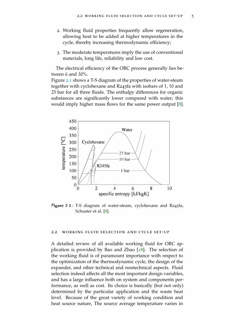
The electrical efficiency of the ORC process generally lies be-tween 6 and 30%.Figure 2.1 shows a T-S diagram of the properties of water-steamtogether with cyclohexane and R245fa with isobars of 1, 10 and25 bar for all three fluids. The enthalpy differences for organicsubstances are significantly lower compared with water; thiswould imply higher mass flows for the same power output [8].
Figure 2.1.: T-S diagram of water-steam, cyclohexane and R245fa,Schuster et al. [8].
2.2 working fluid selection and cycle set-up
A detailed review of all available working fluid for ORC ap-plication is provided by Bao and Zhao [18]. The selection ofthe working fluid is of paramount importance with respect tothe optimization of the thermodynamic cycle, the design of theexpander, and other technical and nontechnical aspects. Fluidselection indeed affects all the most important design variables,and has a large influence both on system and components per-formance, as well as cost. Its choice is basically (but not only)determined by the particular application and the waste heatlevel. Because of the great variety of working condition andheat source nature, The source average temperature varies in
2.2 working fluid selection and cycle set-up 6
a huge range of possible values: from low-temperature heatsource of 80 ◦C (namely, geothermal or solar collector [19, 20]),to high temperature of 500 ◦C heat source (e.g. biomass).
ORC cycles enable the use of once-trough boilers, which avoidssteam drums and recirculation. This is due to the relativelysmaller density difference between vapour and liquid for highmolecular weight organic fluids [9].
It can be said that, from a theoretical viewpoint, all kinds oforganic and inorganic fluids could be used in a ORC system.
Despite the multiplicity of the working fluid studies, no sin-gle fluid has been identified as optimal for a “generic” ORCcycle [18]. This is because:
1. The extent of fluid candidates varies;
2. Different types of heat source and working conditionslead to different optimal working fluids;
3. Different performance indicators result in different bestworking fluid.
To sum up, there is not a working fluid suitable for any or-ganic Rankine cycle system. At the same time, working fluidselection should also consider other aspects apart from thermo-dynamic performance and system economy, such as the maxi-mum and minimum bearable temperature and system pressure,expander design, fluid cost, toxicity, flammability, global warm-ing potential (GWP), availability and so on.
For a general approach, from a viewpoint of thermodynamiccycle performance and turboexpander feasibility, it is desirableto employ organic fluids formed by complex molecules (largeheat capacity) and with high critical temperature. Indeed, dueto the positive slope of their saturation curve in the T-S dia-gram, the vapour expansion in the turbine is completely dry;thus, high superheating in order to avoid liquid in the exhaustvapour is not necessary any more. In addition, for each organicfluid, there is a maximum available temperature due to chem-ical instability problems [21]. However, high superheating ofthe vapour is favourable for better efficiencies1, but this couldlead to very large heat exchangers due to the low value of heatexchange coefficient [9]. If the fluid is “too dry”, the expandedvapour will leave the turbine substantially “superheated”, sothat more heat needs to be theoretically released in the con-denser.
1 When optimizing an ORC it is important for efficiency to reach the highestaverage heat addition temperature consistent with the temperature of theheat source; thus, organic working fluids that are stable at temperatures upto 500 ◦C are desirable [9].
2.3 turboexpanders for organic rankine cycles 7
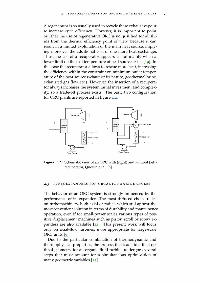
A regenerator is so usually used to recycle these exhaust vapourto increase cycle efficiency. However, it is important to pointout that the use of regenerative ORC is not justified for all flu-ids from the thermal efficiency point of view, because it canresult in a limited exploitation of the main heat source, imply-ing moreover the additional cost of one more heat exchanger.Thus, the use of a recuperator appears useful mainly when alower limit on the exit temperature of heat source exists [19]. Inthis case the recuperator allows to rescue more heat, increasingthe efficiency within the constraint on minimum outlet temper-ature of the heat source (whatever its nature, geothermal brine,exhausted gas flow etc.). However, the insertion of a recupera-tor always increases the system initial investment and complex-ity, so a trade-off process exists. The basic two configurationfor ORC plants are reported in figure 2.2.
Figure 2.2.: Schematic view of an ORC with (right) and without (left)recuperator, Quoilin et al. [9].
2.3 turboexpanders for organic rankine cycles
The behavior of an ORC system is strongly influenced by theperformance of its expander. The most diffused choice relieson turbomachinery, both axial or radial, which still appear themost convenient solution in terms of durability and manteinenceoperation, even if for small-power scales various types of pos-itive displacement machines such as piston scroll or screw ex-panders are also available [22]. This present work will focusonly on axial-flow turbines, more appropriate for large-scaleORC units [9].
Due to the particular combination of thermodynamic andthermophysical properties, the process that leads to a final op-timal geometry for an organic-fluid turbine undergoes severalsteps that must account for a simultaneous optimization ofmany geometric variables [23].

2.3 turboexpanders for organic rankine cycles 8
From the turbine design point of view, most of organic fluidsexhibit small enthalpy drop, low speed of sound, large expan-sion and volumetric flow rate ratio. The contemporary occur-rence of small enthalpy drop (leading to low number of stages)and high volume ratio for organic fluid yields a larger variationof volumetric flow rate per stage than those usually adopted insteam and gas turbine stages.
Fundamentals of turbomachinery theory are comprehensivelydiscussed in Osnaghi [10] or in Saravanamuttoo et al. [24]. Herefollows a brief summary of the main used parameters in thecontext of this present work.
2.3.1 Turbine efficiency
When dealing with turbine stages, it is common practice to ac-count for two different definitions of efficiency: total-to-totaland total-to-static efficiency. For a turbine, the first one is de-fined as follows [10]:
ηtt =H01 −H03H01 −H03is
(2.1)
while the total-to-static efficiency is defined as:
ηts =H01 −H03H01 −H3is
(2.2)
where the suffix “0” indicates a total condition. The differ-ence between these two efficiencies relies in the different waythese parameters account for the outlet velocity: the first oneaccounts for the exit kinetic energy as a component to be stillrecoverable, while the second one, conversely, considers it anenergy loss. Due to its definition itself, the total-to-total effi-ciency appears to be more suitable for the inner stages of a tur-bine; on the contrary, for a single-stage turbine, as well as forthe last stage of multi-stage turbine, the total-to-static versionseems the best alternative since no kinetic energy is recoveredin a following stage.However, when inserting a turbine in a cycle model, the total-to-total efficiency appears to be a more suitable definition sinceit can account also for the velocity recovery and the frictionpressure loss in the diffuser [24].
Two more expressions are defined: isoentropic efficiency andpolytropic efficiency.The first one is defined as:
ηis =∆H13∆H13,is
(2.3)

2.3 turboexpanders for organic rankine cycles 9
The second one can be defined as the isoentropic efficiency ofan infinitesimal expansion: the difference between isoentropicand polytropic efficiency, is this latter one accounts for reheatoccurring during fluid expansion: while passing through tur-bine channels and expanding, the viscous losses acts as an heat-ing on the fluid, which leads to a dilatation and hence to bothan increase of work exchanged by the stage and by the follow-ing one in a multistage machine; the difference in the two finalpower outputs is called reheat effect. The topic is exhaustivelydiscussed in Beccari [25]; here it is just reported that, for aninfinitesimal expansion, the two definitions lead to the same re-sult, because the recovery work Lrec tends to zero. For a finiteexpansion, conversely, it is possible to estimate a slightly highervalue of power output, due to the contribution of Lrec.
According to what previously reported, in this thesis work itwas chosen to employ the total-to-total efficiency as the valueto maximize in the turbine-design optimization process.
2.3.2 Velocity triangles
Figure 2.3.: Sketch of the three conventional surfaces in turbomachin-ery study, Osnaghi [10].
Fluid flow in turbomachinery is usually analysed by meansof three conventional surfaces (see fig. 2.3):
• Blade-to-blade surface (S1 area in figure 2.3): this is thesurface of the main flux;
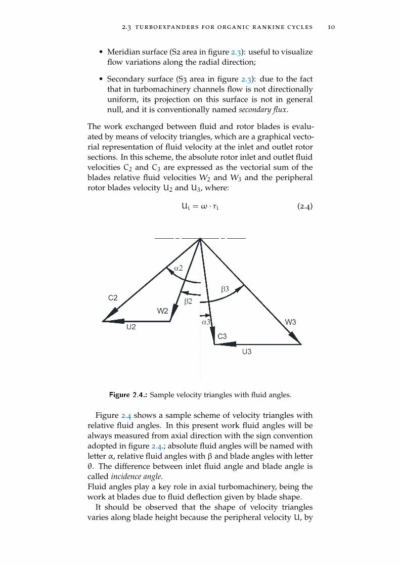
2.3 turboexpanders for organic rankine cycles 10
• Meridian surface (S2 area in figure 2.3): useful to visualizeflow variations along the radial direction;
• Secondary surface (S3 area in figure 2.3): due to the factthat in turbomachinery channels flow is not directionallyuniform, its projection on this surface is not in generalnull, and it is conventionally named secondary flux.
The work exchanged between fluid and rotor blades is evalu-ated by means of velocity triangles, which are a graphical vecto-rial representation of fluid velocity at the inlet and outlet rotorsections. In this scheme, the absolute rotor inlet and outlet fluidvelocities C2 and C3 are expressed as the vectorial sum of theblades relative fluid velocities W2 and W3 and the peripheralrotor blades velocity U2 and U3, where:
Ui = ω · ri (2.4)
Figure 2.4.: Sample velocity triangles with fluid angles.
Figure 2.4 shows a sample scheme of velocity triangles withrelative fluid angles. In this present work fluid angles will bealways measured from axial direction with the sign conventionadopted in figure 2.4.; absolute fluid angles will be named withletter α, relative fluid angles with β and blade angles with letterθ. The difference between inlet fluid angle and blade angle iscalled incidence angle.Fluid angles play a key role in axial turbomachinery, being thework at blades due to fluid deflection given by blade shape.
It should be observed that the shape of velocity trianglesvaries along blade height because the peripheral velocity U, by
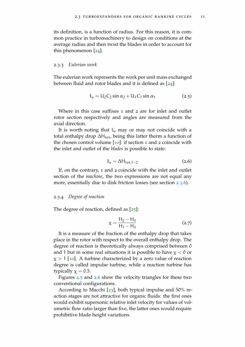
2.3 turboexpanders for organic rankine cycles 11
its definition, is a function of radius. For this reason, it is com-mon practice in turbomachinery to design on conditions at theaverage radius and then twist the blades in order to account forthis phenomenon [24].
2.3.3 Eulerian work
The eulerian work represents the work per unit mass exchangedbetween fluid and rotor blades and it is defined as [24]:
łu = U2C2 sinα2 +U1C1 sinα1 (2.5)
Where in this case suffixes 1 and 2 are for inlet and outletrotor section respectively and angles are measured from theaxial direction.
It is worth noting that lu may or may not coincide with atotal enthalpy drop ∆Htot, being this latter therm a function ofthe chosen control volume [10]: if section 1 and 2 coincide withthe inlet and outlet of the blades is possible to state:
łu = ∆Htot,1−2 (2.6)
If, on the contrary, 1 and 2 coincide with the inlet and outletsection of the machine, the two expressions are not equal anymore, essentially due to disk friction losses (see section 2.3.6).
2.3.4 Degree of reaction
The degree of reaction, defined as [25]:
χ =H2 −H3H1 −H3
(2.7)
It is a measure of the fraction of the enthalpy drop that takesplace in the rotor with respect to the overall enthalpy drop. Thedegree of reaction is theoretically always comprised between 0and 1 but in some real situations it is possible to have χ < 0 orχ > 1 [10]. A turbine characterized by a zero value of reactiondegree is called impulse turbine, while a reaction turbine hastypically χ = 0.5.
Figures 2.5 and 2.6 show the velocity triangles for these twoconventional configurations.
According to Macchi [23], both typical impulse and 50% re-action stages are not attractive for organic fluids: the first oneswould exhibit supersonic relative inlet velocity for values of vol-umetric flow ratio larger than five, the latter ones would requireprohibitive blade height variations.
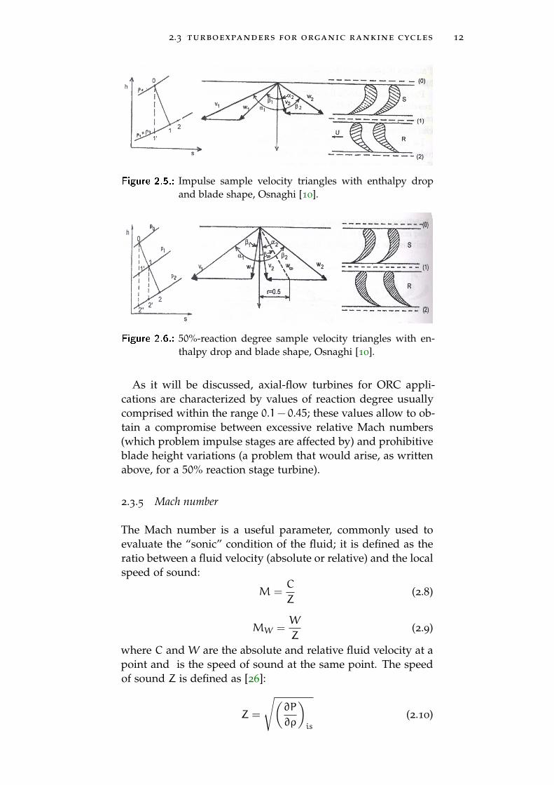
2.3 turboexpanders for organic rankine cycles 12
Figure 2.5.: Impulse sample velocity triangles with enthalpy dropand blade shape, Osnaghi [10].
Figure 2.6.: 50%-reaction degree sample velocity triangles with en-thalpy drop and blade shape, Osnaghi [10].
As it will be discussed, axial-flow turbines for ORC appli-cations are characterized by values of reaction degree usuallycomprised within the range 0.1− 0.45; these values allow to ob-tain a compromise between excessive relative Mach numbers(which problem impulse stages are affected by) and prohibitiveblade height variations (a problem that would arise, as writtenabove, for a 50% reaction stage turbine).
2.3.5 Mach number
The Mach number is a useful parameter, commonly used toevaluate the “sonic” condition of the fluid; it is defined as theratio between a fluid velocity (absolute or relative) and the localspeed of sound:
M =C
Z(2.8)
MW =W
Z(2.9)
where C and W are the absolute and relative fluid velocity at apoint and is the speed of sound at the same point. The speedof sound Z is defined as [26]:
Z =
√(∂P
∂ρ
)is
(2.10)

2.3 turboexpanders for organic rankine cycles 13
if M < 1, the velocity of the fluid is lesser than the speed ofsound and the flow is said subsonic, by definition.If M > 1 the flow is supersonic. Depending on the Mach num-ber level different design concepts and different correlationsmust be used.
2.3.6 Turbine losses
In turbomachinery theory the losses evaluation procedure isnot unified but every method accounts for the following physi-cal phenomena:
• Profile (or primary) losses: the main purpose of bladesin turbomachinery is to deflect the flux in the tangen-tial direction in order to obtain a useful torque at shaft.Losses are mainly linked to fluid deflection in the blade-to-blade surface; profile losses result from the boundarylayer growth on the surface of the profile and from theaccompanying friction and blockage effects. Moreover,the finite thickness of the trailing edge leads to mixingwakes and recirculating vortexes, so an optimal distancebetween two following blade channels exists [10]. From adimensionless analysis, a representative parameter of thisphenomena is the chord/pitch ratio b/s, also defined assolidity σ: for very low values of this parameter the de-flection imposed on the fluid takes place in a too shortlength, with risk of flow detachment; conversely, whenthis parameter is too high the blade chord is too long withexcessive friction losses.
• Secondary losses: they are basically due to energy trans-fer from blade-to-blade surface to secondary surface; thisis mainly the consequence of the turning of the spanwisevelocity gradients near the endwalls. The secondary flowsare perpendicular to the main flow direction and have avery complex character. These losses are the most diffi-cult to describe because of their highly 3-D configurationand interconnection of the singles phenomena that occurin secondary surface. These losses have an increasing rel-ative influence when the blade height decreases with re-spect to blade channel section. This effect is more signif-icant in rotors [25], where also tip clearance losses2 mustbe accounted for.
2 Leakage of mass flow rate at tip, separated from the main flow due to therotation of the rotor that induces pressure difference between pressure andsuction surface of the blade.

2.3 turboexpanders for organic rankine cycles 14
• Three-dimensional effects: as already observed, the shapeof velocity triangles varies along blade height because theperipheral velocity U is a function of radius. Due to thisvariation, flow configuration varies along blade height. 3-D effects introduces weak specific loss mechanisms (suchas the effects of flaring), but the variation of velocity trian-gles can significantly increase the incidence angle, with asubsequent increment in profile losses. The influence of 3-D effect is quite complex and is also dependent on bladedesign. From a dimensionless point of view, the most rep-resentative parameter is the blade height/average diame-ter ratio h/Dm [23]: for high values of this parameter, typ-ical of last stages in steam turbines [24], these effects canintroduce significant losses, so blades are usually twistedto account for variation of blade angles along the radialcoordinate.
It is common practice in turbomachinery to account for lossesby means of subtractive coefficients that reduce the efficiency.In the present thesis work, the loss coefficients Xi are predictedby making use of Craig and Cox method [4], that appears tobe the most suitable and complete loss evaluation process forthe purpose of this work [22, 23, 27, 28]. In this section themain concepts of this methodology are summarized (for furtherdetails see Craig and Cox [4]).The total amount of losses that occur in a axial-flow turbine isdivided into two groups, listed in table 2.1.
Table 2.1.: List of turbine losses according to Craig and Cox method,Craig and Cox [4].
Group 1 Group 2
Nozzle profile loss Nozzle gland leakage loss
Rotor profile loss Rotor tip clearance loss
Nozzle secondary loss Wetness loss
Rotor secondary loss Lacing wire loss
Nozzle annulus loss (lap andcavity)
Partial admission loss
Rotor annulus loss (lap, cavityand annulus)
Disc windage loss

2.3 turboexpanders for organic rankine cycles 15
The total-to-total efficiency is defined as:
ηtt =lu
lu +∑
(group 1 losses)
−∑
(group 2 efficiencydebits) (2.11)
This approach basically relies on the fact that the work atblades is obtained by the change in tangential momentum, butthe energy released by the fluid is even more, due to the fric-tion on blade profiles and blade wakes (profile losses), frictionon walls at tip and hub and other secondary phenomena, lossesdue to sudden enlargements in fluid path or wall cavities (an-nulus losses). Losses of group 2, contrarily, account for the factthat not all the fluid passes through rotor blades, because ofleakage through diaphragms glands and tip clearances. In ad-dition, partial admission, windage and bearing losses reduceeven more the final work at shaft. This second group can bemore easily treated as a an efficiency debt to be subtracted to a“blade efficiency”, that accounts only for both nozzle and rotorprofile together with secondary losses3.
3 It could be said that group 1 losses only account for flow channel losses,without being concern with mass flow leakage or any other loss external toblade channel.

3M E T H O D O L O G Y
In this chapter a description of the case of study is given andthe adopted methodology and used models are described.
3.1 case of study : the draugen offshore platform
The Draugen oil field is located in the North Sea, situated ap-proximately 150 km north of Kristiansund in Norway, 200 Kmfar from the Arctic Circle. The Draugen oil field is operated byNorske Shell, which also owns a 26.2% stake in the field. Theremaining stake is held by Petoro (47.88%), BP Norge (18.36%)and Chevron (7.56%). The field was shut down in February2010 due to cold weather and extreme winds. Shell is yet toresume operations at the facility [11]. The Garn West reservoiris connected to the Draugen platform by a 3.3 km-long pipeline.The pipeline laid via the Garn West reservoir connects the Rogndeposit to the project platform. While the oil extracted from thefield is transferred to a floating loading buoy, the associated gasis transported to processing plant at Karsto by means of the As-gard Transport pipeline.
Figure 3.1.: Draugen field location, Offshore Technology [11].
The energy requirement of the platform (normal and peakload) is supplied by three Siemens SGT-500 gas turbines. TheSiemens SGT-500 industrial gas turbine is a light-weight, high-efficiency, heavy duty gas turbine in the 15 MW to 20 MW
16
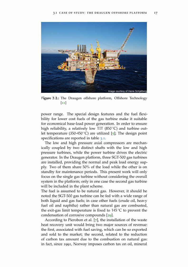
3.1 case of study : the draugen offshore platform 17
Figure 3.2.: The Draugen offshore platform, Offshore Technology[11]
power range. The special design features and the fuel flexi-bility for lower cost fuels of the gas turbine make it suitablefor economical base-load power generation. In order to ensurehigh reliability, a relatively low TIT (850 ◦C) and turbine out-let temperature (350-450 ◦C) are utilized [5]; The design pointspecifications are reported in table 3.1.
The low and high pressure axial compressors are mechan-ically coupled by two distinct shafts with the low and highpressure turbines, while the power turbine drives the electricgenerator. In the Draugen platform, three SGT-500 gas turbinesare installed, providing the normal and peak load energy sup-ply. Two of them share 50% of the load while the other is onstandby for maintenance periods. This present work will onlyfocus on the single gas turbine without considering the overallsystem in the platform; only in one case the second gas turbinewill be included in the plant scheme.The fuel is assumed to be natural gas. However, it should benoted the SGT-500 gas turbine can be fed with a wide range ofboth liquid and gas fuels; in case other fuels (crude oil, heavyfuel oil and naphtha) rather than natural gas are combusted,the exit-gas limit temperature is fixed to 145 ◦C to prevent thecondensation of corrosive compounds [29].
According to Pierobon et al. [7], the installation of the wasteheat recovery unit would bring two major sources of revenue:the first, associated with fuel saving, which can be so exportedand sold to the market; the second, related to the reductionof carbon tax amount due to the combustion on natural gas:in fact, since 1991, Norway imposes carbon tax on oil, mineral

3.2 general overview of turbine design code 18
Table 3.1.: Design point specifications for Siemens SGT-500 [5]
Low pressure compressor stages 10
High pressure compressor stages 8
Low pressure turbine stages 1
High pressure turbine stages 2
Power turbine stages 3
Turbine inlet temperature (TIT ) 850 ◦CExhaust gas temperature 376 ◦CExhaust gas mass flow 93.5 kg/sNet power output 17.014 MWHeat rate 11312 kJ/kWh
Fuel Naphta, crude oil, heavyfuel oil, bio oil, naturalgas, syngas
fuel and natural gas with rates based on fuels carbon content[30]. Thus, the new method would reduce the carbon tax costassociated with the release of CO
2due to combustion of natural
gas.
3.2 general overview of turbine design code
In this section a description of the used single-stage turbine-design code is given. For a more exhaustive and detailed dis-cussion see Gabrielli [12].
As previously anticipated, the whole turbine design processrelies on a set of eight parameters, together with some otherrequirements. These input variables are listed in table 3.2.
Figure 3.3 reports two blades with the main geometric pa-rameters and relative nomenclature that will be used in thiswork.
In addition to the ones listed in table 3.2, some other values,such as the surface roughness and trailing edge thickness mustbe given in input. However, these numbers have been chosento be consistent with the best available technology and are keptconstant during the whole work1. A complete list of all theinput requirements is reported in table B.1 in appendix B.
1 The value of Mach number that makes nozzle geometry switch from con-vergent to convergent-divergent is set to 1.4, in accordance to Osnaghi [10].A turbulent flow configuration (Re > 106) is also always assumed.The rotor inlet/nozzle outlet blade height ratio hhh has been set to one toensure the minimum annulus loss for controlled expansion, according toCraig and Cox’ figure 19 reported in appendix B [4].
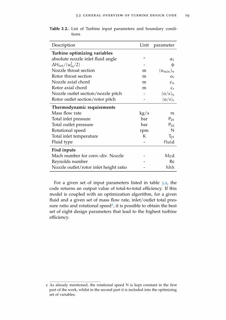
3.2 general overview of turbine design code 19
Table 3.2.: List of Turbine input parameters and boundary condi-tions
Description Unit parameter
Turbine optimizing variablesabsolute nozzle inlet fluid angle ° α1∆Htot/(u
2m/2) - ψ
Nozzle throat section m (omin)nRotor throat section m orNozzle axial chord m cnRotor axial chord m crNozzle outlet section/nozzle pitch - (o/s)nRotor outlet section/rotor pitch - (o/s)r
Thermodynamic requirementsMass flow rate kg/s m
Total inlet pressure bar P01Total outlet pressure bar P03Rotational speed rpm N
Total inlet temperature K T01Fluid type - fluid
Fixd inputsMach number for conv.-div. Nozzle - Mcd
Reynolds number - Re
Nozzle outlet/rotor inlet height ratio - hhh
For a given set of input parameters listed in table 3.2, thecode returns an output value of total-to-total efficiency. If thismodel is coupled with an optimization algorithm, for a givenfluid and a given set of mass flow rate, inlet/outlet total pres-sure ratio and rotational speed2, it is possible to obtain the bestset of eight design parameters that lead to the highest turbineefficiency.
2 As already mentioned, the rotational speed N is kept constant in the firstpart of the work, whilst in the second part it is included into the optimizingset of variables.
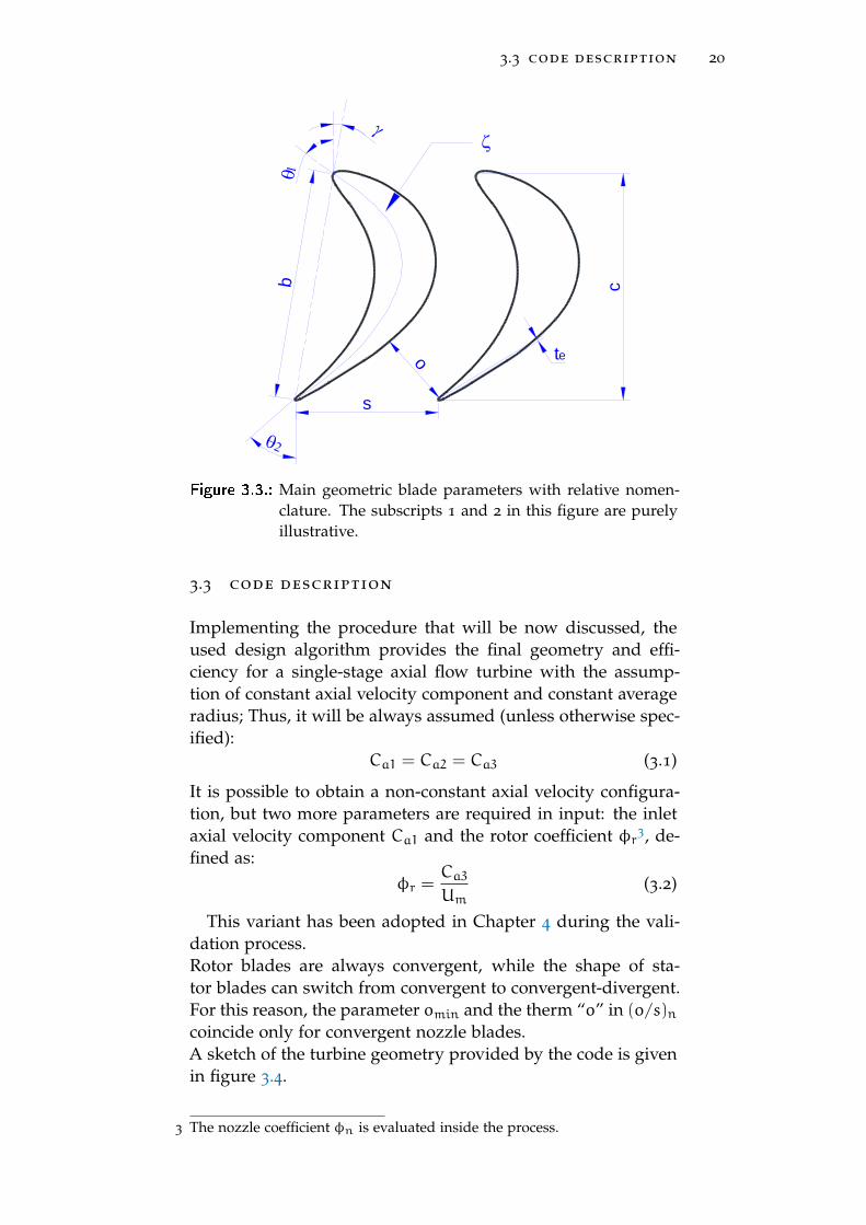
3.3 code description 20
b c
s
teo
Figure 3.3.: Main geometric blade parameters with relative nomen-clature. The subscripts 1 and 2 in this figure are purelyillustrative.
3.3 code description
Implementing the procedure that will be now discussed, theused design algorithm provides the final geometry and effi-ciency for a single-stage axial flow turbine with the assump-tion of constant axial velocity component and constant averageradius; Thus, it will be always assumed (unless otherwise spec-ified):
Ca1 = Ca2 = Ca3 (3.1)
It is possible to obtain a non-constant axial velocity configura-tion, but two more parameters are required in input: the inletaxial velocity component Ca1 and the rotor coefficient φr3, de-fined as:
φr =Ca3Um
(3.2)
This variant has been adopted in Chapter 4 during the vali-dation process.Rotor blades are always convergent, while the shape of sta-tor blades can switch from convergent to convergent-divergent.For this reason, the parameter omin and the therm “o” in (o/s)ncoincide only for convergent nozzle blades.A sketch of the turbine geometry provided by the code is givenin figure 3.4.
3 The nozzle coefficient φn is evaluated inside the process.
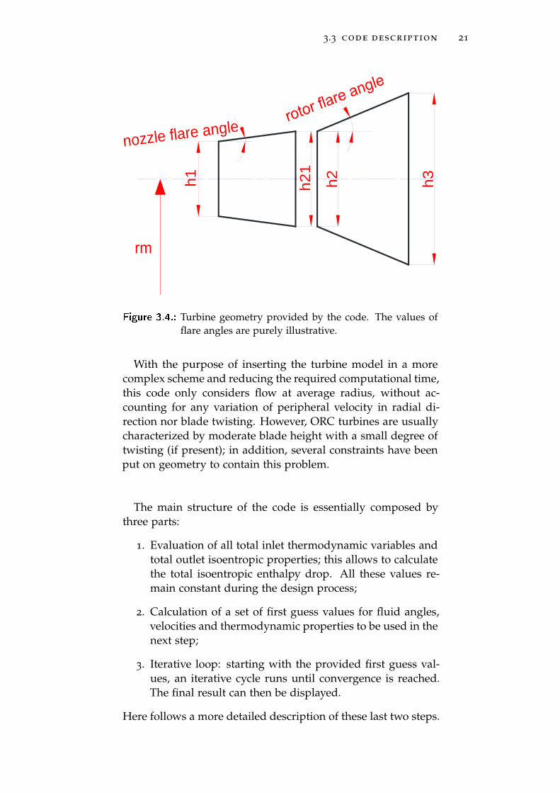
3.3 code description 21
h1
h2
1
h2
h3
nozzle flare angle
rm
Figure 3.4.: Turbine geometry provided by the code. The values offlare angles are purely illustrative.
With the purpose of inserting the turbine model in a morecomplex scheme and reducing the required computational time,this code only considers flow at average radius, without ac-counting for any variation of peripheral velocity in radial di-rection nor blade twisting. However, ORC turbines are usuallycharacterized by moderate blade height with a small degree oftwisting (if present); in addition, several constraints have beenput on geometry to contain this problem.
The main structure of the code is essentially composed bythree parts:
1. Evaluation of all total inlet thermodynamic variables andtotal outlet isoentropic properties; this allows to calculatethe total isoentropic enthalpy drop. All these values re-main constant during the design process;
2. Calculation of a set of first guess values for fluid angles,velocities and thermodynamic properties to be used in thenext step;
3. Iterative loop: starting with the provided first guess val-ues, an iterative cycle runs until convergence is reached.The final result can then be displayed.
Here follows a more detailed description of these last two steps.

3.3 code description 22
3.3.1 First guess values calculation
This part of the code simply aims at obtaining an approximatedset of values for fluid angles, velocities and thermodynamicproperties, that will be subsequently updated in the iterativeloop. Providing a first guess value for ηtt, it is possible to obtaina first guess value for the work per unit mass and then, fromψ, the velocity U. By assuming fluid flow angles coincidentwith blade angles, α2 and β3 are evaluated by the followingexpressions:
α2 = arccos(os
)n
(3.3)
β3 = arccos(os
)r
(3.4)
The remaining velocities are obtained by trigonometric rela-tions achievable from velocity triangles [12, 24].
With the first guess values for all the kinematic variables itis now possible to start a subroutine that provides a set of firstguess values for thermodynamic properties. The detailed de-scription of this process is provided by Gabrielli [12] and isnot reported here, being quite complex, cumbersome and notuseful for the general understanding of code structure.
3.3.2 Iterative loop
The iterative loop is composed by the following steps:
1. Calculation of nozzle blade opening with Deich formula[31]: if the flow is supersonic, this step allows to switch toa converging-diverging shape of nozzle blades;
2. Blades and fluid angles evaluation: θ21 and θ3 are ob-tained by means of the following expressions:
θ21 = arccos(os
)n
(3.5)
and
θ3 = arccos(os
)r
(3.6)
for a subsonic case, fluid angles are calculated with Ainleyand Mathieson correlation [32], whereas the Vavra corre-lation is used for supersonic cases [33];
3. Updating velocity calculation with fluid angles;

3.3 code description 23
4. Thermodynamic properties and Mach numbers estima-tion;
5. Turbine geometry calculation (flare angles, blade height)by means of continuity equation;
6. Updating Mach numbers with Kacker-Okapuu correlation[34] to improve Craig and Cox method for supersonicflow;
7. Losses estimation procedure with Craig and Cox method[4];
8. calculation of total-to-total turbine efficiency;
9. Calculation of the difference with respect to the previousiteration and update of values to start the loop again.
The iterative loop stops when the difference between the newobtained efficiency and the one calculated in the preceding iter-ations goes below a given tolerance, set at 10−4.
3.3.3 Optimization process
For a given fluid, mass flow rate, total inlet temperature andpressure ratio, it is possible to include the turbine code into amore complex function in order to obtain the best geometricconfiguration that produces the highest efficiency. It is pos-sible to fulfil this goal by coupling the turbine code with anoptimization algorithm, called “genetic algorithm”. A compre-hensive description of this process is provided by Obitko [35];a general overview is given in appendix A. Here it is only re-ported that, providing a set of upper and lower bound valuesfor each parameter to be optimized, the algorithm looks for thebest combination of optimizing parameters that maximizes (orminimizes) a certain function.The general syntax has the following expression:
[OP] = f (fopt, [LB], [UB],GAoptions) (3.7)
where:
• fopt is the function to be optimized;
• [OP] is the set of optimizing parameters that maximizesor minimizes a certain function fopt;
• [LB] and [UB] are the lower and upper bound arrays ofvalues;
• GAoptions is the set of required options necessary to thegenetic algorithm (see appendix A)

3.3 code description 24
3.3.4 Constraints on the solution
To provide acceptable solutions both for a physical and techno-logical prospective, some constraints on geometry and thermo-dynamics have to be given. This basically turns into an upperand lower bound for the optimizing variables, listed in table 3.3and in some other constraints to be respected by the obtainedsolutions, provided in table 3.4; these conditions have substan-tially been established by Macchi and Perdichizzi [27].
Table 3.3.: List of upper and lower bound for the nine turbine designparameters to be optimized.
Parameter Lower bound Upper bound Unit
α1 −15 15 °ψ 2 6 −
(omin)n 0.002 0.1 m
or 0.002 0.1 m
cn 0.01 0.1 m
cr 0.01 0.1 m
(o/s)n 0.224 0.7 −
(o/s)r 0.224 0.7 −
N (if optimized) 2000 12000 rpm
Table 3.4.: Other constraints on turbine geometry.
Parameter Lower bound Upper bound Unit
MW2 0 0.8 −
MW3 0 1.4 −
zn 10 100 −
zr 10 100 −
FLn −25 25 °FLr −25 25 °hi/Dm 0.001 0.25 −
ci/Dm 0 0.2 −
Some comments are necessary:
• Rotor inlet relative Mach number MW2 is limited to sub-sonic values to avoid unique incidence configuration andto ensure the validity of loss correlation [4]; outlet rela-tive Mach number MW3 is limited due to the hypothesis

3.4 influence analysis of optimizing variables 25
of the assumed converging shape of rotor blades; the re-striction on Mach number, however, goes in the directionof the best efficiency, because supersonic inlet velocitieswith high fluid deflection yield high losses [23].
• Flare angles are limited to ensure a limited influence ofradial effects and restrain the efficiency reduction in off-design conditions;
• h/Dm is limited to restrain the three-dimensional effects,related to peripheral velocity variation with blade height(whose influence this model does not account for).
• The limits on axial chords, throat and opening sections,as well as the number of blades, are due to technologicalreasons [23].
• The limit on (o/s)n and (o/s)r is due to contain the max-imum deflection ∆α and ∆β. Excessive values of fluiddeflection increase the aerodynamic lift per blade and canlead to fluid flow detachment [27];
• The upper and lower bound for ψ are not “limiting” it:from a preliminary set of optimization results it was seenthat optimal values for this coefficient are always com-prised between 2.5 and 5. The given upper and lowerbounds allow the algorithm find the best value being cer-tain it is within the given range.
3.4 influence analysis of optimizing variables
Here follows a more comprehensive description of the influ-ence and effect each design parameter has on the final output.All the optimizing parameters have a certain influence, eventhough three of them have a more relevant role compared tothe others. The following charts have been obtained with asample set of optimizing parameters, mass flow rate and inletturbine temperature (see table B.3 in appendix B) and choosingcyclopentane as test fluid.The design parameters were made vary in pairs of two withinthe correspondent upper and lower bound values4, keeping allthe other input values constant. The effect of each couple of pa-rameters has been evaluated in charts showing the variation of
4 It is necessary to note that, even though each design parameter has his ownupper and lower bound, it is not possible to make one (or two) parameter(s)vary within its/their whole possible range keeping all the other values con-stant. Indeed, for a given fluid, inlet turbine temperature, pressure ratio andmass flow rate, not all the possible combinations of design parameters areacceptable, even with larger constraints.
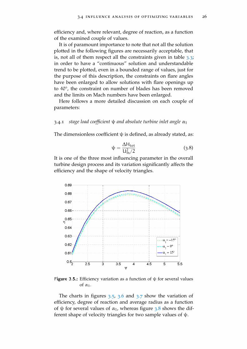
3.4 influence analysis of optimizing variables 26
efficiency and, where relevant, degree of reaction, as a functionof the examined couple of values.
It is of paramount importance to note that not all the solutionplotted in the following figures are necessarily acceptable, thatis, not all of them respect all the constraints given in table 3.3;in order to have a “continuous” solution and understandabletrend to be plotted, even in a bounded range of values, just forthe purpose of this description, the constraints on flare angleshave been enlarged to allow solutions with flare openings upto 40°, the constraint on number of blades has been removedand the limits on Mach numbers have been enlarged.
Here follows a more detailed discussion on each couple ofparameters:
3.4.1 stage load coefficient ψ and absolute turbine inlet angle α1
The dimensionless coefficient ψ is defined, as already stated, as:
ψ =∆Htot
U2m/2(3.8)
It is one of the three most influencing parameter in the overallturbine design process and its variation significantly affects theefficiency and the shape of velocity triangles.
Figure 3.5.: Efficiency variation as a function of ψ for several valuesof α1.
The charts in figures 3.5, 3.6 and 3.7 show the variation ofefficiency, degree of reaction and average radius as a functionof ψ for several values of α1, whereas figure 3.8 shows the dif-ferent shape of velocity triangles for two sample values of ψ.

3.4 influence analysis of optimizing variables 27
Figure 3.6.: Variation of reaction degree as a function of ψ for severalvalues of α1.
Figure 3.7.: Variation of average radius as a function of ψ for severalvalues of α1.
Figure 3.8.: velocity triangles for ψ = 2 (black) and ψ = 5.5 (red).
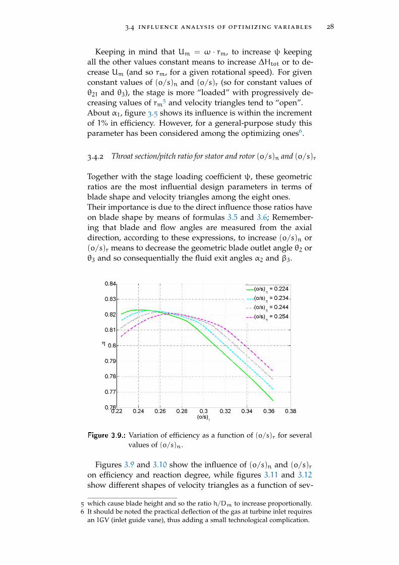
3.4 influence analysis of optimizing variables 28
Keeping in mind that Um = ω · rm, to increase ψ keepingall the other values constant means to increase ∆Htot or to de-crease Um (and so rm, for a given rotational speed). For givenconstant values of (o/s)n and (o/s)r (so for constant values ofθ21 and θ3), the stage is more “loaded” with progressively de-creasing values of rm5 and velocity triangles tend to “open”.About α1, figure 3.5 shows its influence is within the incrementof 1% in efficiency. However, for a general-purpose study thisparameter has been considered among the optimizing ones6.
3.4.2 Throat section/pitch ratio for stator and rotor (o/s)n and (o/s)r
Together with the stage loading coefficient ψ, these geometricratios are the most influential design parameters in terms ofblade shape and velocity triangles among the eight ones.Their importance is due to the direct influence those ratios haveon blade shape by means of formulas 3.5 and 3.6; Remember-ing that blade and flow angles are measured from the axialdirection, according to these expressions, to increase (o/s)n or(o/s)r means to decrease the geometric blade outlet angle θ2 orθ3 and so consequentially the fluid exit angles α2 and β3.
Figure 3.9.: Variation of efficiency as a function of (o/s)r for severalvalues of (o/s)n.
Figures 3.9 and 3.10 show the influence of (o/s)n and (o/s)ron efficiency and reaction degree, while figures 3.11 and 3.12show different shapes of velocity triangles as a function of sev-
5 which cause blade height and so the ratio h/Dm to increase proportionally.6 It should be noted the practical deflection of the gas at turbine inlet requires
an IGV (inlet guide vane), thus adding a small technological complication.

3.4 influence analysis of optimizing variables 29
Figure 3.10.: Variation of reaction degree as a function of (o/s)r forseveral values of (o/s)n
Figure 3.11.: Different velocity triangles for a constant valueof (o/s)r=0.238 with (o/s)n=0.224 (black) and(o/s)n=0.374 (red).
Figure 3.12.: Different velocity triangles for a constant valueof (o/s)n=0.224 with (o/s)r=0.224 (black) and(o/s)r=0.364 (red).

3.4 influence analysis of optimizing variables 30
eral combinations of (o/s)n and (o/s)r. As written above, anincrease of (o/s)n causes θ2 and so α2 to decrease, as shown infigure 3.11. This basically means that the fluid is less deflectedand/or expanded in the nozzle, which causes the degree of re-action to increase.For the same reason, in figure 3.12, an increase of (o/s)r causesθ3 and so β3 to decrease, and that means the fluid is, in propor-tion, less deflected and/or expanded in the rotor: this causes areduction in reaction degree. This is confirmed by the trendsin figure 3.10, where the degree of reaction χ decreases for in-creasing values of (o/s)r. This chart also shows the influence of(o/s)n that induces the opposite effect: indeed, for a fixed valueof (o/s)r, the higher (o/s)n, the higher the reaction degree.
3.4.3 Throat sections (omin)n, or and axial chords cn, cr
The remaining parameters whose influence has not been anal-ysed yet play a somehow different role in the whole turbinedesign and optimization process. Figures 3.13 and 3.14 showthe effect of these parameters on efficiency.
Figure 3.13.: Efficiency variation as a function of or for several valuesof nozzle throat section.
The values of throat sections and axial chords do not modifydirectly the shape of velocity triangles, but the effect of theirvariation is considered inside the code while estimating all theremaining geometric variables, most of whom are successivelyreceived as an input in the losses evaluation procedure: for ex-ample, the values of on and or are used to evaluate nozzle androtor pitch (and so the number of blades in stator and rotor)
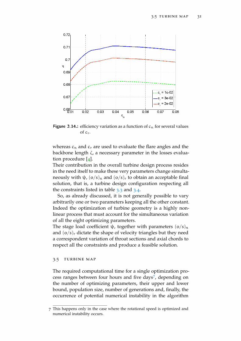
3.5 turbine map 31
Figure 3.14.: efficiency variation as a function of cn for several valuesof cr.
whereas cn and cr are used to evaluate the flare angles and thebackbone length ζ, a necessary parameter in the losses evalua-tion procedure [4].Their contribution in the overall turbine design process residesin the need itself to make these very parameters change simulta-neously with ψ, (o/s)n and (o/s)r to obtain an acceptable finalsolution, that is, a turbine design configuration respecting allthe constraints listed in table 3.3 and 3.4.
So, as already discussed, it is not generally possible to varyarbitrarily one or two parameters keeping all the other constant.Indeed the optimization of turbine geometry is a highly non-linear process that must account for the simultaneous variationof all the eight optimizing parameters.The stage load coefficient ψ, together with parameters (o/s)nand (o/s)r dictate the shape of velocity triangles but they needa correspondent variation of throat sections and axial chords torespect all the constraints and produce a feasible solution.
3.5 turbine map
The required computational time for a single optimization pro-cess ranges between four hours and five days7, depending onthe number of optimizing parameters, their upper and lowerbound, population size, number of generations and, finally, theoccurrence of potential numerical instability in the algorithm
7 This happens only in the case where the rotational speed is optimized andnumerical instability occurs.

3.6 cycle model 32
(see section 5.5 and appendix A). The insertion in a completecycle model would imply the addition of at least two more cyclevariables to be optimized (evaporation pressure and turbine in-let temperature), with a further increase in computational time.It also should be considered that, when optimizing a thermody-namic cycle, one is initially more interested in knowing the bestefficiency achievable for an expander with certain inlet condi-tions than knowing its complete geometry. Moreover, as it willbe discussed in section 3.6.2, the creation of a map allows to ob-tain the convergence in the iterative loop of internal recuperator.Thus, it was chosen to optimize expander geometry separatelyand subsequently integrate the obtained map into the cycle.For a single fluid, turbine inlet temperature and rotational speed,many optimizations have been performed to plot turbine effi-ciency as a function of mass flow rate and inlet/outlet pressureratio; The mass flow rate was varied between 10 and 200 kg/s,with a variation of pressure ratio between 5 and 44. The resultsare reported and discussed in chapter 5.In the complete cycle model, the map is embed into a functionto return turbine efficiency as follows:
ηtt = f (m,Pr) (3.9)
Whenever the values of mass flow rate and pressure ratio arenot directly provided in the map, this function interpolates lin-early between the two closest values of these variables.
3.6 cycle model
For the given case of study, an organic Rankine bottoming cyclemodel has been set up. The structure of the cycle with thenomenclature that will be used is reported in figure 3.15, whilea complete list of cycle input requirements is reported in tableB.2 in appendix B. Fluid properties will be referred to withsubscript from 1 to 8, while gas temperature will be indicatedwith subscript from A to D.
For a simpler approach that does not affect the structure ofthe problem, no pressure losses have been taken into accountthroughout the cycle; the exhausted gas have been consideredas ideal with constant specific heat, which allows to write:
∆Hgas = cp ·∆T (3.10)
In the most general case, the complete optimization of a ther-modynamic cycle would imply the simultaneous research forthe best combination of the following parameters:
• Turbine inlet temperature;

3.6 cycle model 33
Figure 3.15.: ORC plant scheme.
• Turbine inlet pressure: this parameter influences signifi-cantly cycle efficiency, mass flow rate and primary heatexchanger (PHE) area and volume [7, 19];
• Minimum cycle pressure;
• Pinch point temperature difference in PHE (∆Tpp): from athermodynamic point of view, the lower the pinch point,the higher the heat recovery and the overall plant effi-ciency, but the higher the PHE area and cost as well [36];
• Pinch point temperature difference in regenerator (∆Tpp,rec):it is the temperature difference between points 2 and 8
(see figure 3.15 and 3.16). This parameter influences theamount of recovered heat and its optimization is impor-tant in presence of a limit on minimum outlet temperatureof heat source, since a proper recuperator design allowsto reach the best compromise between thermodynamic ef-ficiency and exploitation of the particular heat source;
• Selection of working fluid.
For this present work, the number of cycle optimizing parame-ters has been reduced due to the following considerations:

3.6 cycle model 34
• Cyclopentane has been chosen as the working fluid, being,according to Pierobon et al. [7], the optimal choice for thiscase of study;
• Without pressure losses there are only two pressure val-ues, namely the evaporation pressure and the condensa-tion one; this latter tends always to the minimum possi-ble value within the constraints given by thermodynamicfluid properties and operative considerations.In this present work the condensing pressure has alwaysbeen fixed to 1 bar, in order to avoid air leakage into thepipes [9], a problem that would also lead to rapid decom-position of organic working fluid [21, 37];
• From a thermodynamic point of view, the higher the max-imum cycle temperature (that is, the turbine inlet temper-ature), the higher the cycle efficiency. However, as dis-cussed by Ginosar et al. [21], due to chemical instability is-sues, there is a maximum available operative temperaturefor the chosen fluid, found to be 513.15K. It was chosen tobuild the map for this value of turbine inlet temperature.This assumption implies to work with a constant value ofT6.
• Both ∆Tpp and ∆Tpp,rec have been fixed to the minimumvalue provided by Pierobon et al. [7] and reported in ta-ble B.2 in appendix B. Inside the cycle calculation pro-cess, if necessary, the location of the ∆Tpp is made switchautomatically from evaporator inlet to recuperator outlet.Figure 3.16 shows a sample T-S diagram for these twoconfigurations.
It is worth noting this cycle model only provides subcriticalconfigurations. It was chosen to limit the analysis just to thisconfiguration because, for the chosen fluid, a supercritical cyclemodel would require values of turbine pressure ratio that aretoo large for being effectively managed in a single-stage turbine.Moreover, supercritical configurations for ORC are still underexperimental study and not easily commercially available.For this reason, the maximum available turbine pressure hasbeen fixed to 0.9 · Pcr8.
8 The critical pressure of cyclopentane is Pcr = 45.71 bar. Thus, this limitcorresponds to a maximum available pressure ratio of 41.

3.6 cycle model 35
Figure 3.16.: Sample T-S diagram with two heat sources and two dif-ferent locations of ∆Tpp.
3.6.1 Fluid properties
Both the aformentioned Coolprop and Refprop® codes require asimilar syntax to calculate the desired thermodynamic proper-ties [14, 15]; the general expression is:
A(i) = f (A,B,Bi,C,Ci, fluid name) (3.11)
where “i” is the desired value of the property A and both Band C are two more thermodynamic properties and Bi and Ciare their correspondent value in “i”.For example, the enthalpy in point 7 in figure 3.15 can be eval-uated by the following expression:
H7 = f (H, T , T7,P,P7, fluid name) (3.12)
While estimating thermodynamic properties in saturated condi-tion, the thermodynamic title substitutes the second parameter.
3.6.2 ORC model description
Attending to nomenclature shown in figure 3.15 and 3.16, thecycle model is developed as follows:
1. For a given P6 and T6, the thermodynamic properties atpoint 6, 5, 4 and 1 are obtained. With the first assump-tion of ∆Tpp located on evaporator inlet (point 4), the ex-hausted gas temperature TC is evaluated as:
TC = T4 +∆Tpp

3.6 cycle model 36
and the mass flow rate mORC is obtained through the en-ergy balance of superheater and evaporator sections:
mgas · cp,gas · (TA − TC) = mORC · (H6 −H4)
Now it is possible to calculate also TB from the super-heater energy balance:
mgas · cp,gas · (TA − TB) = mORC · (H6 −H5)
2. A pump function is created to calculate pump consump-tion and point 2 properties as follows:
(H2,S2, T2,Lp) = f (P1,P2,ηp, ρ1, fluid) [kJ/kg] (3.13)
where Lp and H2 are respectively calculated as:
Lp =P2 − P1ρ1 · ηp
(3.14)
H2 = H1 + ηp · Lp (3.15)
3. The turbine map function is made run as in eq. 3.9. Theproperties for isoentropic point 7is are evaluated and tur-bine work is obtained as:
Lt = ηt · (H6 −H7is) = (H6 −H7) [kJ/kg]
This allows also to calculate H7.Now that H7 is known, all the remaining properties atpoint 7 are calculated;
4. It is now possible to calculate T8 as:
T8 = T2 +∆Tpp,rec
and so the remaining thermodynamic properties in point8. Through the recuperator energy balance H3 is obtainedas:
H3 = H2 + qrec
where qrec = H7 −H8. Now it is possible to obtain the re-maining thermodynamic properties in point 3 and obtainthe exhausted gas exit temperature TD as:
TD = TC − mORC ·(
H4 −H3mgas · cp,gas
)5. The location of the pinch point is checked:
if TD − T3 < ∆Tpp, a new cycle calculation begins with the∆Tpp located in point 3 (recuperator exit);

3.6 cycle model 37
6. The new mass flow rate has to be evaluated from the pri-mary heat exchanger energy balance:
mgas · cp,gas · (TA − TD) = mORC · (H6 −H3)
In this case it is not possible to calculate mORC until H3is known. But H3 is a function of the recuperator energybalance which in turn, depends on H7, calculated withthe turbine map function that needs mORC to be run. Aniterative process is so performed, described as follows:
• For a first guess turbine efficiency the properties ofpoint 7 are evaluated;
• With H7, through the recuperator energy balance, H3is obtained, and so TD, being now TD = T3 +∆Tpp;
• mORC is now obtained from equation in step 6;
• the map function is called and the new turbine effi-ciency is obtained and updated; this loop is repeateduntil a convergence on turbine efficiency set at 10−3
is reached.
7. Finally the output power is calculated as:
Wout = mORC · (ηgen · Lt − Lp) [kW] (3.16)
while the plant efficiency is defined as:
ηORC =Wout
Qmax,gas(3.17)
where Qmax,gas = mgas · cp,gas · (TA − TD,min) and TD,minis the minimum allowed exhausted gas exit temperature.
For each test performed, the results are compared to the onesobtained with a similar ORC plant model that considers a con-stant turbine efficiency ηt = 0.8. The structure of this secondmodel is the same as the one just described, with the assump-tion, of course, that expander efficiency is known (and given asan input parameter), so no iterative loop is required to evaluatethe mass flow rate in the equation in step 6.
It is worth noting the turbine map has proved to be a usefultool to ensure the convergence of the internal loop: during thisroutine, the mass flow rate fluctuates and it has been observedthat, if the entire turbine optimization process is inserted in thecycle model, it is not possible to reach convergence, because anychange in mass flow rate should be followed by a simultaneousvariation of all the turbine optimizing parameters, and this isnot possible. Thus, if the map had not been used, the algorithmwould have always stopped without reaching convergence.

3.7 optimization accounting for rotational speed 38
3.7 optimization accounting for rotational speed
In the second part of this work, a new turbine map has beengenerated, considering also the rotational speed as an optimiz-ing parameter. The complete set of input requirements is thesame provided in table B.1 in appendix B, but considering Namong the optimizing parameters with the upper and lowerbound set to 2000 and 12000 rpm (see also table 3.3). Alsoin this case, the outlet pressure was fixed to 1 bar, turbine in-let temperature was fixed to 513.15 ◦C and mass flow rate wasvaried between 10 and 200 kg/s for values of pressure ratiobetween 5 and 44.
The new map was then inserted into the organic Rankinecycle model and the output power was evaluated as describedin section 3.6, with the only addition of a gearbox efficiencyfixed to 0.96 [20].
3.8 turbine techno-economic optimization
To find out whether and to what extent different expander opti-mization processes can affect the optimal design and eventuallycycle configuration, a techno-economic optimization has beenperformed: in this process, the specific cost (in e/kW) was cho-sen as the parameter to be minimized instead of maximizingthe total-to-total turbine efficiency.
The specific cost was computed by means of the cost functiondeveloped by Astolfi et al. [20]:
Ct = C0 ·(n
n0
)(0.5)
·(SP
SP0
)1.1(3.18)
where n is number of stages (always one, in this present work),n0 = 2, C0 = 1230 · 103 e and SP0 = 0.18 m. SP is the sizeparameter, defined as:
SP =
√Vout
∆H3/4is,stage
[m] (3.19)
The electric power produced by the turbine is computed as:
Wt = ηgen · mORC ·∆Htot (3.20)
and so the specific cost is defined as:
Cspec,t =CturbWturb
(3.21)
in e/kW.The specific cost was optimized for three different values of

3.9 estimation of gearbox profitability 39
pressure ratio, as a function of mass flow rate and comparedwith the specific cost obtained for the conventional thermody-namic optimization.
3.9 estimation of gearbox profitability
A techno-economic estimation has been performed to evaluatethe profitability of a gearbox insertion.The difference between the present value of cash inflows andthe present value of cash outflows is called “net present value”(NPV) [38] and it is mathematically defined as [39]:
NPV =
n∑i=0
Ri(1+ q)i
− Itot (3.22)
where Ri is the annual revenue, q is the interest factor, n isthe equipment lifespan and Itot is the total investment cost. Asstated by Pierobon et al. [7], the total investment cost can becalculated as a function of the sum of purchase equipment cost(PEC) of plant components:
Itot = 3.7 · (PECHE + PECp + PECturb + PECcond+ PECIR + PECgen + PECgear) (3.23)
For the present case of study, as previously introduced, twomajor sources of income with the installation of the ORC unitare expected: the first is associated with the fuel saving, thesecond with the CO
2tax.
The power produced by the ORC unit allows to reduce theload of the other gas turbine operating on the platform: thesaved fuel can then be exported and sold to the marked, be-coming an additional revenue.
According to turbine data provided in tables 3.1 and 3.5, thesaved mass flow rate of fuel can be calculated as:
msf =WORC,net · 3600LHVf ·HR
(3.24)
where WORC,net is the net output power of waste heat recoveryunit, LHV is the low heating value of natural gas and HR is thegas turbine heat rate.
The annual revenue Rsf due to saved fuel (in e/year) is esti-mated as follows:
Rsf = msf · hu · 3600 ·Cng (3.25)
where hu is the utilization factor [7] and Cng is the price ofnatural gas [40].

3.9 estimation of gearbox profitability 40
Table 3.5.: Parameter assumed for the economic analysis
parameter Symbol Unit Value
Natural gas price [40] Cgn NOK/MMBTU 24.04Energy conversion fac-tor [41]
- GJ/MMBTU 1.054615
utilization factor [7] hu hours/year 7000
Low heating value [7] LHV MJ/kg 48.530Carbon tax [30] CT NOK/tCO2
410
Carbon dioxide emis-sion rate [42]
CO2 e.r. kgCO2/kgCH4 2.75
Maintenance [7] Ma - 0.9Equipment lifespan [7] n years 20
Interest factor [7] q - 10%Conversion factor [43] - e/NOK 0.1224Generator efficiency[7]
ηgen - 0.98
Gearbox efficiency ηgear - 0.96
The income RCO2(in e/year) related to the CO
2saving is
computed as:
RCO2= msf · hu · 3600 ·CO2 e.r. ·
CT
1000(3.26)
where CO2 e.r. is the carbon dioxide emission rate and CT is thecarbon tax.The annual revenue Ri is therefore defined as:
Ri = Rs.fuel,i + RCO2,i (3.27)
According to equation 3.23, a complete techno-economic anal-ysis must account for all plant components and it is out of thepurpose of this present work. However, in order to evaluate theprofitability of a gearbox purchase, a full analysis is not neces-sary, being an estimation of the sought information given bythe following difference:
NPVdiff = NPVgear −NPVno−gear (3.28)
where the subscripts gear and no-gear respectively indicate aplant configuration where the gearbox is considered and not.In fact, for a given evaporation pressure, it is possible to con-sider heat exchangers dimensions approximately constant forthe two cases in pair, being the heat exchanger dimensions in-fluenced by pressure and mass flow rate, and being this latterapproximately the same for the two configurations once estab-lished the pressure ratio (see also section 5). Following this

3.9 estimation of gearbox profitability 41
approach, considering the pump as a fixed-cost component aswell, all these values basically disappear in equation 3.28; theresult is positive when the gearbox insertion is convenient.
Thus, in this present work only turbine, electrical generatorand gearbox cost are considered. The first one is calculatedwith equation 3.18, while the second one is calculated as sug-gested by Astolfi et al. [20]:
Cgen = C0 ·(Wel
Wel,0
)0.67(3.29)
where Wel,0 = 5000 kW and C0 = 200 ke. In case a gearboxis present, its cost is considered equal to 40% of the electricalgenerator cost.
It was chosen to assume a value of 96% for gearbox efficiency,thereby reducing of one point the value of 97% adopted by As-tolfi et al. [20]: indeed, as a consequence of the lack of moredetailed information about this component, it was chosen toconsider a slightly less effective performance.

4V E R I F I C AT I O N A N D VA L I D AT I O N O F T H EC O D E
In this chapter the performances of the code are tested andcompared with two cases:
1. A similar computational code, capable of producing anoptimized turbine design;
2. A set of experimental data regarding a four-stage turbineprovided by Evers and Kötzing [6].
In all the analyses performed in this chapter the code has notbeen coupled with the optimization routine and the φr coef-ficient, as well as the inlet axial velocity Ca1, is provided asan input value; this allows to have a non-constant axial veloc-ity component throughout the stage, which is the real physicalconfiguration for both the examined cases.
4.1 verification with axtur code
AXTUR is a code developed by the department of energy inPolytechnic of Milan [44]. Provided the requested input data,it can produce the optimal design of an axial-flow turbine withone, two or three stages. It employs the same correlation as theexamined single-stage code to estimate fluid angles and losses.
It was chosen to reproduce a subsonic case with the valueslisted in table 4.1.
These values, together with the useful results given by AX-TUR output, provide the input values for the single-stage modelcomputational code. The purpose of this test is to check if, pro-vided the correct input data, the turbine code can reproducethe same results as AXTUR. It should be noted that, just likethe employed design code, AXTUR does not account for anyradial equilibrium problem.
The complete set of input values for the single-stage modelcode is listed in table 4.2, while both the output values obtainedby the two codes are provided and compared in table 4.3. Therelative error is defined as:
ε =
∣∣∣∣ξobtained − ξaxturξaxtur
∣∣∣∣ · 100 (4.1)
where ξ is a generic parameter.Figure 4.1 shows the velocity triangles for this case.
42

4.1 verification with axtur code 43
Table 4.1.: Provided input data for AXTUR
Parameter Unit Value
Fluid − Ideal gasmolecular configuration − biatomicMM kg/kmol 28.4m kg/s 10
T01 K 1123.15P01 bar 2
P03 bar 1
N rpm 10000
Number of stages − 1
α1 ° 0
Re − 105
Mcd − 1.4
Table 4.2.: Input data provided for turbine code.
Parameter Unit Value
Fluid − airm kg/s 10
T01 K 1123.15P01 bar 2
P03 bar 1
N rpm 10000
Re − 105
Mcd − 1.4α1 ° 0
ψ − 2.1457(omin)n m 0.01091or m 0.01139cn m 0.0354cr m 0.0354(os )n − 0.25086(os )r − 0.31762φr − 0.3475Ca1 m/s 89.2hhh − 1.04
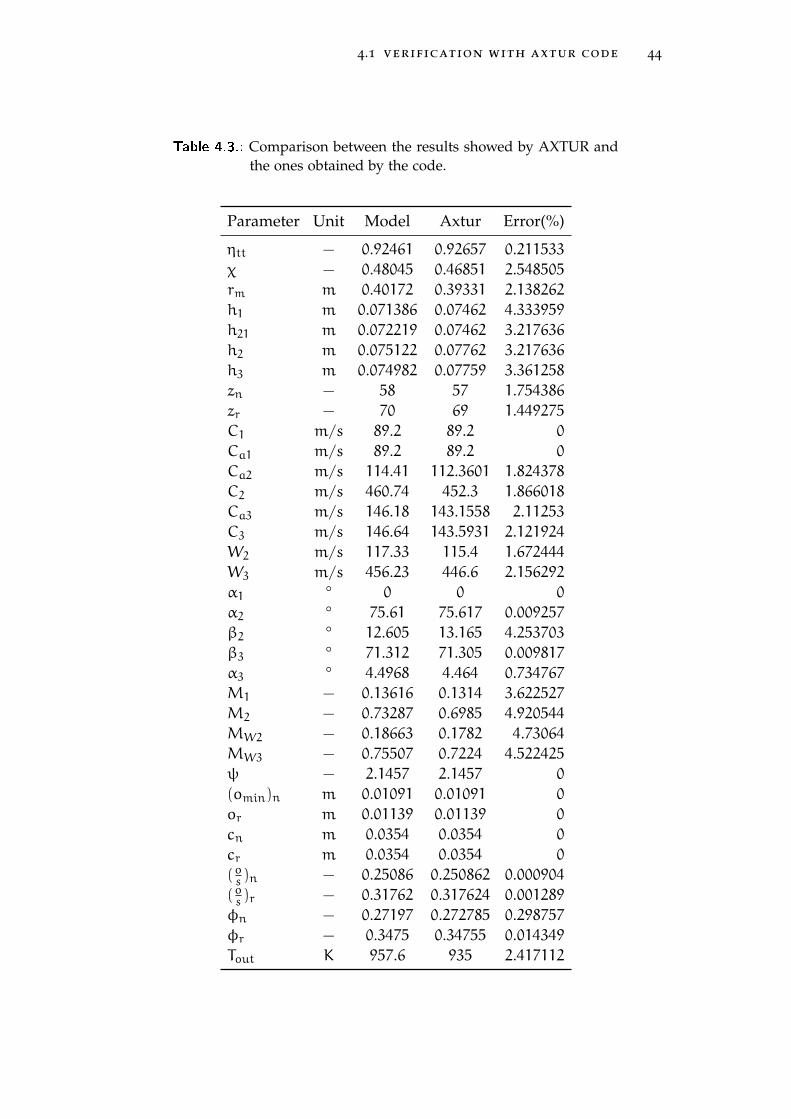
4.1 verification with axtur code 44
Table 4.3.: Comparison between the results showed by AXTUR andthe ones obtained by the code.
Parameter Unit Model Axtur Error(%)
ηtt − 0.92461 0.92657 0.211533χ − 0.48045 0.46851 2.548505rm m 0.40172 0.39331 2.138262h1 m 0.071386 0.07462 4.333959h21 m 0.072219 0.07462 3.217636h2 m 0.075122 0.07762 3.217636h3 m 0.074982 0.07759 3.361258zn − 58 57 1.754386zr − 70 69 1.449275C1 m/s 89.2 89.2 0
Ca1 m/s 89.2 89.2 0
Ca2 m/s 114.41 112.3601 1.824378C2 m/s 460.74 452.3 1.866018Ca3 m/s 146.18 143.1558 2.11253C3 m/s 146.64 143.5931 2.121924W2 m/s 117.33 115.4 1.672444W3 m/s 456.23 446.6 2.156292α1 ° 0 0 0
α2 ° 75.61 75.617 0.009257β2 ° 12.605 13.165 4.253703β3 ° 71.312 71.305 0.009817α3 ° 4.4968 4.464 0.734767M1 − 0.13616 0.1314 3.622527M2 − 0.73287 0.6985 4.920544MW2 − 0.18663 0.1782 4.73064MW3 − 0.75507 0.7224 4.522425ψ − 2.1457 2.1457 0
(omin)n m 0.01091 0.01091 0
or m 0.01139 0.01139 0
cn m 0.0354 0.0354 0
cr m 0.0354 0.0354 0
(os )n − 0.25086 0.250862 0.000904(os )r − 0.31762 0.317624 0.001289φn − 0.27197 0.272785 0.298757φr − 0.3475 0.34755 0.014349Tout K 957.6 935 2.417112

4.2 validation with evers and kötzing 45
Figure 4.1.: Velocity triangles for AXTUR test case.
As reported in table 4.3, the obtained results are in agreementwith the ones provided by AXTUR. The highest error is the oneconcerning the inlet blade height (about 4.33 %).Some words should also be dedicated to the different values ob-tained for the outlet temperature Tout; this discrepancy could beattributed to the different assumptions made about fluid naturein the two codes: indeed, AXTUR utilizes an ideal-gas model,while for the computational code the Refprop database has beenused. This can lead to slightly different values for the thermo-dynamic properties that can also affect Mach number and bladeheight, being it evaluated through the mass flow rate continuityequation.
4.2 validation with evers and kötzing
Evers and Kötzing [6] describe a test case of a four-stage airaxial-flow turbine. A meridional view of the machine section isreported in figure 4.2.
Figure 4.2.: Flow path with measuring stations 0− 4, Evers and Kötz-ing [6].

4.2 validation with evers and kötzing 46
Table 4.4.: Turbine design data, Evers and Kötzing [6]
Parameter Unit Value
N rpm 7500
m kg/s 7.8Pin bar 2.6Tin K 413
Pout bar 1.022Tout K 319
η − 0.913Coupling power kW 703
For the inlet of each stage and for turbine outlet several mea-surements are available in nine different points on blade height;thus, for each station, nine values of total pressure, static pres-sure, total temperature, absolute velocity, absolute flow angleand radial flow angle are provided. The turbine was basicallydesigned to have the same blade section in all stages at a givenradius. The blades are twisted according to the free-vortex the-ory with a 50% reaction degree in the middle section of the laststage. The geometry of stator and rotor blades is reported inappendix C. For several heights along the blade (five for thenozzle and six for the rotor) the values of the following param-eters are provided:
• Stagger angle;
• Solidity: σ = b/s, where b is the profile chord and s is theblade pitch;
• profile chord b;
• blade angles θ1, θ21, θ2, θ3;
These values, the thermodynamic measurements and the tur-bine input values listed in table 4.4, allow to evaluate all theinput parameters necessary for the code. It has been chosento validate the code just for the first and fourth stage of theturbine, being them the ones with the highest amount of exper-imental data.
All the input values requested by the code have been extrap-olated using the thermodynamic values at the average radiusfor the particular stage; it is worth noting that the blade heightvalues which the geometric parameters are given for, do not co-incide with the height values used to provide thermodynamicdata (see also appendix C); it was so necessary to interpolate
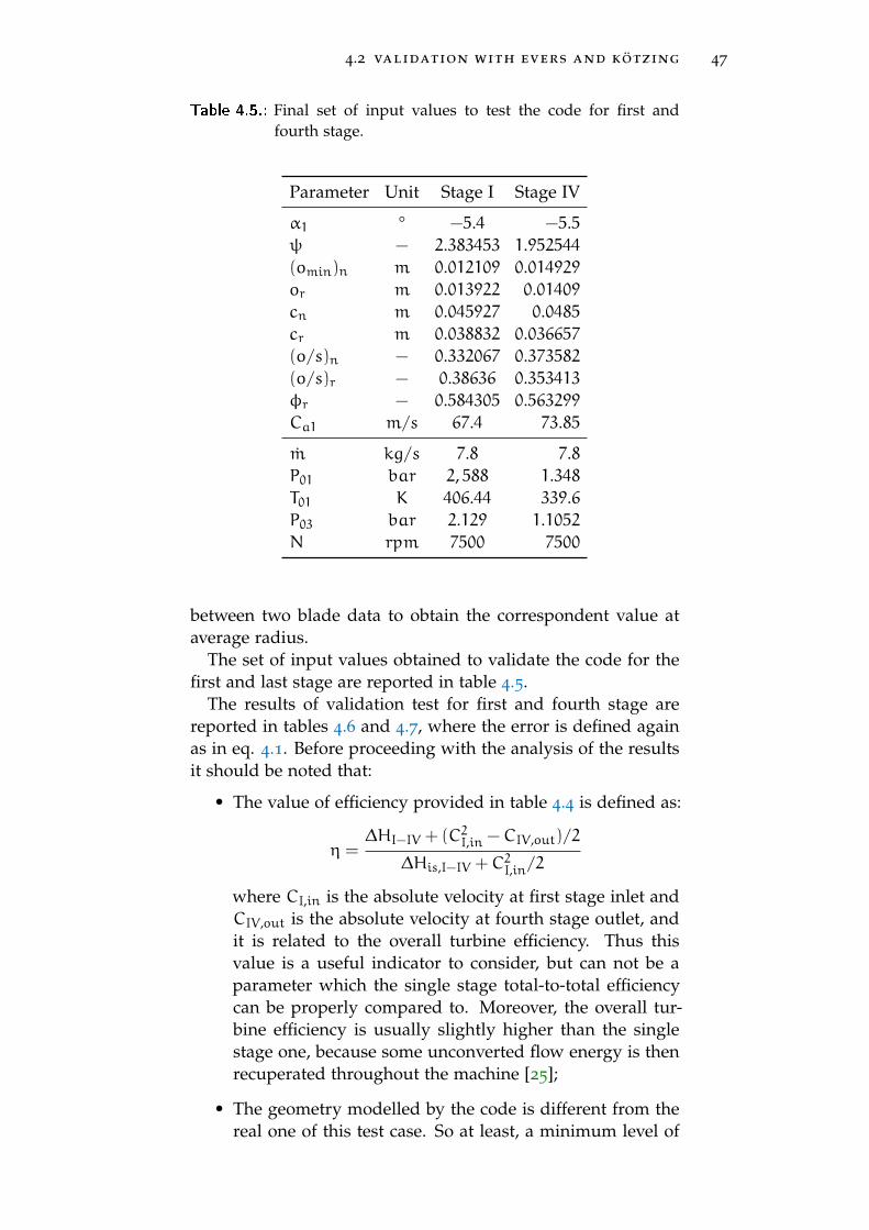
4.2 validation with evers and kötzing 47
Table 4.5.: Final set of input values to test the code for first andfourth stage.
Parameter Unit Stage I Stage IV
α1 ° −5.4 −5.5ψ − 2.383453 1.952544(omin)n m 0.012109 0.014929or m 0.013922 0.01409cn m 0.045927 0.0485cr m 0.038832 0.036657(o/s)n − 0.332067 0.373582(o/s)r − 0.38636 0.353413φr − 0.584305 0.563299Ca1 m/s 67.4 73.85
m kg/s 7.8 7.8P01 bar 2, 588 1.348T01 K 406.44 339.6P03 bar 2.129 1.1052N rpm 7500 7500
between two blade data to obtain the correspondent value ataverage radius.
The set of input values obtained to validate the code for thefirst and last stage are reported in table 4.5.
The results of validation test for first and fourth stage arereported in tables 4.6 and 4.7, where the error is defined againas in eq. 4.1. Before proceeding with the analysis of the resultsit should be noted that:
• The value of efficiency provided in table 4.4 is defined as:
η =∆HI−IV + (C2I,in −CIV ,out)/2
∆His,I−IV +C2I,in/2
where CI,in is the absolute velocity at first stage inlet andCIV ,out is the absolute velocity at fourth stage outlet, andit is related to the overall turbine efficiency. Thus thisvalue is a useful indicator to consider, but can not be aparameter which the single stage total-to-total efficiencycan be properly compared to. Moreover, the overall tur-bine efficiency is usually slightly higher than the singlestage one, because some unconverted flow energy is thenrecuperated throughout the machine [25];
• The geometry modelled by the code is different from thereal one of this test case. So at least, a minimum level of
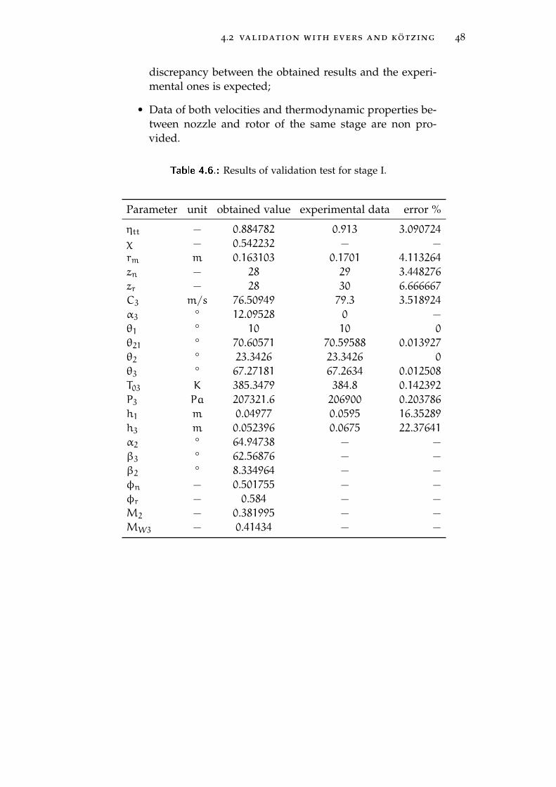
4.2 validation with evers and kötzing 48
discrepancy between the obtained results and the experi-mental ones is expected;
• Data of both velocities and thermodynamic properties be-tween nozzle and rotor of the same stage are non pro-vided.
Table 4.6.: Results of validation test for stage I.
Parameter unit obtained value experimental data error %
ηtt − 0.884782 0.913 3.090724χ − 0.542232 − −
rm m 0.163103 0.1701 4.113264zn − 28 29 3.448276zr − 28 30 6.666667C3 m/s 76.50949 79.3 3.518924α3 ° 12.09528 0 −
θ1 ° 10 10 0
θ21 ° 70.60571 70.59588 0.013927θ2 ° 23.3426 23.3426 0
θ3 ° 67.27181 67.2634 0.012508T03 K 385.3479 384.8 0.142392P3 Pa 207321.6 206900 0.203786h1 m 0.04977 0.0595 16.35289h3 m 0.052396 0.0675 22.37641α2 ° 64.94738 − −
β3 ° 62.56876 − −
β2 ° 8.334964 − −
φn − 0.501755 − −
φr − 0.584 − −
M2 − 0.381995 − −
MW3 − 0.41434 − −

4.2 validation with evers and kötzing 49
Table 4.7.: Results of validation test for stage IV
Parameter unit obtained value experimental data error %
ηtt − 0.848922 0.913 7.018449χ − 0.721565 0.5 44.31291rm m 0.179183 0.1871 4.231459zn − 28 29 3.448276zr − 28 30 6.666667C3 m/s 83.73556 84.7 1.138653α3 ° 18.87892 5.4 249.6096θ1 ° 10 10 0
θ21 ° 68.06333 68.0626 0.001071θ2 ° −2.8233 −2.8233 0
θ3 ° 69.30377 69.3022 0.002261T03 K 319.8864 319.3 0.183642P3 Pa 101237.4 101200 0.036966h1 m 0.065751 0.0892 26.28781h3 m 0.074611 0.103 27.56209α2 ° 61.73962 − −
β3 ° 64.72768 − −
β2 ° −22.904 − −
φn − 0.437797 − −
φr − 0.563 − −
M2 − 0.356869 − −
MW3 − 0.520362 − −
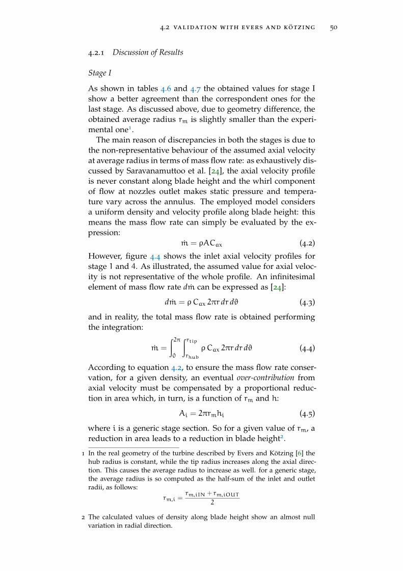
4.2 validation with evers and kötzing 50
4.2.1 Discussion of Results
Stage I
As shown in tables 4.6 and 4.7 the obtained values for stage Ishow a better agreement than the correspondent ones for thelast stage. As discussed above, due to geometry difference, theobtained average radius rm is slightly smaller than the experi-mental one1.
The main reason of discrepancies in both the stages is due tothe non-representative behaviour of the assumed axial velocityat average radius in terms of mass flow rate: as exhaustively dis-cussed by Saravanamuttoo et al. [24], the axial velocity profileis never constant along blade height and the whirl componentof flow at nozzles outlet makes static pressure and tempera-ture vary across the annulus. The employed model considersa uniform density and velocity profile along blade height: thismeans the mass flow rate can simply be evaluated by the ex-pression:
m = ρACax (4.2)
However, figure 4.4 shows the inlet axial velocity profiles forstage 1 and 4. As illustrated, the assumed value for axial veloc-ity is not representative of the whole profile. An infinitesimalelement of mass flow rate dm can be expressed as [24]:
dm = ρCax 2πr dr dϑ (4.3)
and in reality, the total mass flow rate is obtained performingthe integration:
m =
∫2π0
∫ rtiprhub
ρCax 2πr dr dϑ (4.4)
According to equation 4.2, to ensure the mass flow rate conser-vation, for a given density, an eventual over-contribution fromaxial velocity must be compensated by a proportional reduc-tion in area which, in turn, is a function of rm and h:
Ai = 2πrmhi (4.5)
where i is a generic stage section. So for a given value of rm, areduction in area leads to a reduction in blade height2.
1 In the real geometry of the turbine described by Evers and Kötzing [6] thehub radius is constant, while the tip radius increases along the axial direc-tion. This causes the average radius to increase as well. for a generic stage,the average radius is so computed as the half-sum of the inlet and outletradii, as follows:
rm,i =rm,iIN + rm,iOUT
2
2 The calculated values of density along blade height show an almost nullvariation in radial direction.
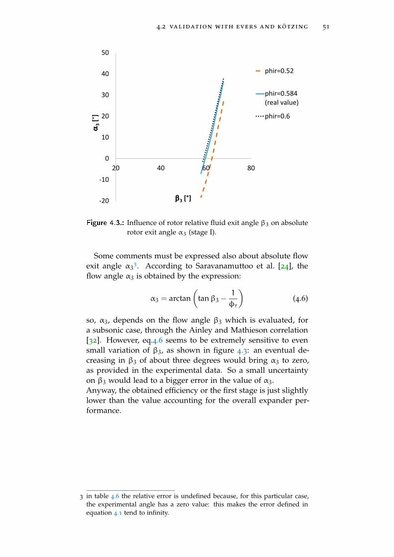
4.2 validation with evers and kötzing 51
-20
-10
0
10
20
30
40
50
20 40 60 80
α3 [
°]
β3 [°]
phir=0.52
phir=0.584(real value)
phir=0.6
Figure 4.3.: Influence of rotor relative fluid exit angle β3 on absoluterotor exit angle α3 (stage I).
Some comments must be expressed also about absolute flowexit angle α33. According to Saravanamuttoo et al. [24], theflow angle α3 is obtained by the expression:
α3 = arctan(
tanβ3 −1
φr
)(4.6)
so, α3, depends on the flow angle β3 which is evaluated, fora subsonic case, through the Ainley and Mathieson correlation[32]. However, eq.4.6 seems to be extremely sensitive to evensmall variation of β3, as shown in figure 4.3: an eventual de-creasing in β3 of about three degrees would bring α3 to zero,as provided in the experimental data. So a small uncertaintyon β3 would lead to a bigger error in the value of α3.Anyway, the obtained efficiency or the first stage is just slightlylower than the value accounting for the overall expander per-formance.
3 in table 4.6 the relative error is undefined because, for this particular case,the experimental angle has a zero value: this makes the error defined inequation 4.1 tend to infinity.

4.2 validation with evers and kötzing 52
Stage IV
The errors obtained for the fourth stage show a bigger discrep-ancy with experimental data (table 4.7): as reported in figure4.4 and 4.5, in this last stage the variation of axial velocity alongradial direction, both for inlet and outlet, is much more signifi-cant than in the first stage. The axial velocity profile is decreas-ing from hub to tip, a phenomenon that the code can not ac-count for with a single axial velocity distribution. Due to this,the error in blade height is more consistent than in the firststage, with a consequent under-estimation of efficiency. Bothfor first and last stage, lower values for Ca1 and φr would bemore representative in terms of overall stage performances andmass flow rate, leading both to higher values for blade lengthand efficiency. Moreover, according to equation 4.6, a lowervalue of φr would also reduce the error in α3.
0.135
0.145
0.155
0.165
0.175
0.185
0.195
0.205
0.215
0.225
50 60 70 80 90
rad
ial c
oo
rdin
ate
[m
]
axial velocity component [m/s]
stage 1 inlet
stage 4 inlet
assumed Vaxfor stage 1
assumed Vaxfor stage 4
Figure 4.4.: Axial velocity profile for inlet section of stage I ad IV.
Finally, it is worth mentioning again that in all the stages, es-pecially in the last ones, the “real” blades are highly twisted toaccount for fluid variation in radial direction and increase theefficiency, an aspect that is not taken into account, as previouslyanticipated, in the employed code.

4.3 conclusions 53
0.135
0.145
0.155
0.165
0.175
0.185
0.195
0.205
0.215
0.225
0.235
50 70 90 110
rad
ial c
oo
rdin
ate
[m
]
axial velocity component [m/s]
Profile of Ca3at stage 1 exit
Profile of Ca3at stage 4 exit
assumed Ca3for stage 1
assumed Ca3for stage 4
Figure 4.5.: Axial velocity profile for outlet section of stage I ad IV.
4.3 conclusions
From the results obtained in this chapter it is possible to statethat:
• The computational code has shown satisfactory accuracywith reliable previous similar models (maximum relativeerror of 4.33%);
• Whenever three-dimensional variations of flux are presentbut still not significantly pronounced, the model is stillcapable of giving acceptable results in terms of efficiency,even if with bigger error in blade geometry, especially inblade height (up to 22%);
• In circumstances when three-dimensional effects are sig-nificant and velocity profile can not be represented byonly one component at mean radius any more, the resultsare not trustable and a more complex approach is neces-sary.However, organic fluid turbines typically exhibit moder-ate blade height, therefore the model is expected to givesatisfactory results in the context of the present work.

5D I S C U S S I O N O F R E S U LT S
In this chapter all the obtained results are reported and dis-cussed.
5.1 turbine maps
5.1.1 Map for constant rotational speed
0 20 40 60 80 100 120 140 160 180 2000.5
0.55
0.6
0.65
0.7
0.75
0.8
0.85
0.9
mass flow rate [kg/s]
η
Pr = 5
Pr = 10
Pr = 15
Pr = 20
Pr = 25
Pr = 30
Pr = 35
Pr = 40
Pr = 44
Figure 5.1.: Turbine efficiency map for constant rotational speed.
The results obtained for the first set of turbine design opti-mizations with N = 3000 rpm are reported in figure 5.1, whichshows the trends of total-to-total efficiency as a function ofmass flow rate and pressure ratio Pr = P01/P03. The efficiencygrows up when the first one increases and the second one de-creases, and its variations are more significant when mass flowrate is lower than 100 kg/s and pressure ratio ranges from 5 to30. Higher values of mass flow rate lead to larger turbine forthe same pressure ratio, with bigger blade channels and reducethe relative influence of boundary layers and secondary losses.
For high values of pressure ratio the iterative loop requiresmore iterations, thereby increasing the overall computationaltime. Moreover, for values of pressure ratio higher than 30, thecurves start showing some fluctuating behaviour. The follow-ing pictures show the trends of the most interesting parameters.In accordance with the results obtained by Macchi [23] the de-gree of reaction (figure 5.2) is, as expected, comprised between0.2 and 0.5. The higher the pressure ratio, the lower the degree
54
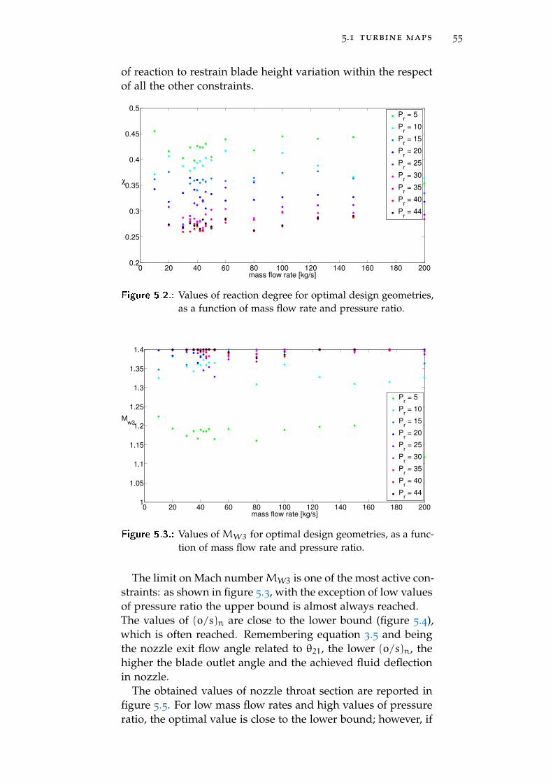
5.1 turbine maps 55
of reaction to restrain blade height variation within the respectof all the other constraints.
0 20 40 60 80 100 120 140 160 180 2000.2
0.25
0.3
0.35
0.4
0.45
0.5
mass flow rate [kg/s]
χ
Pr = 5
Pr = 10
Pr = 15
Pr = 20
Pr = 25
Pr = 30
Pr = 35
Pr = 40
Pr = 44
Figure 5.2.: Values of reaction degree for optimal design geometries,as a function of mass flow rate and pressure ratio.
0 20 40 60 80 100 120 140 160 180 2001
1.05
1.1
1.15
1.2
1.25
1.3
1.35
1.4
mass flow rate [kg/s]
Mw3
Pr = 5
Pr = 10
Pr = 15
Pr = 20
Pr = 25
Pr = 30
Pr = 35
Pr = 40
Pr = 44
Figure 5.3.: Values of MW3 for optimal design geometries, as a func-tion of mass flow rate and pressure ratio.
The limit on Mach numberMW3 is one of the most active con-straints: as shown in figure 5.3, with the exception of low valuesof pressure ratio the upper bound is almost always reached.The values of (o/s)n are close to the lower bound (figure 5.4),which is often reached. Remembering equation 3.5 and beingthe nozzle exit flow angle related to θ21, the lower (o/s)n, thehigher the blade outlet angle and the achieved fluid deflectionin nozzle.
The obtained values of nozzle throat section are reported infigure 5.5. For low mass flow rates and high values of pressureratio, the optimal value is close to the lower bound; however, if

5.1 turbine maps 56
desirable, values of omin smaller than the ones obtained wouldbe impractical in many cases, due to the high number of blades,which often already reaches the maximum admitted value (fig-ure 5.6).
0 20 40 60 80 100 120 140 160 180 200
0.24
0.26
0.28
0.3
0.32
0.34
mass flow rate [kg/s]
(o/s
) n
Pr = 5
Pr = 10
Pr = 15
Pr = 20
Pr = 25
Pr = 30
Pr = 35
Pr = 40
Pr = 44
Figure 5.4.: Values of (o/s)n for optimal design geometries, as afunction of mass flow rate and pressure ratio.
0 20 40 60 80 100 120 140 160 180 200
0.005
0.01
0.015
0.02
0.025
mass flow rate [kg/s]
om
in [
m]
Pr = 5
Pr = 10
Pr = 15
Pr = 20
Pr = 25
Pr = 30
Pr = 35
Pr = 40
Pr = 44
Figure 5.5.: Values of omin for optimal design geometries, as a func-tion of mass flow rate and pressure ratio.

5.1 turbine maps 57
0 20 40 60 80 100 120 140 160 180 20040
50
60
70
80
90
100
mass flow rate [kg/s]
zn
Pr = 5
Pr = 10
Pr = 15
Pr = 20
Pr = 25
Pr = 30
Pr = 35
Pr = 40
Pr = 44
Figure 5.6.: Number of nozzle blades for optimal design geometries,as a function of mass flow rate and pressure ratio.
5.1.2 Turbine map for optimized rotational speed
If rotational speed is considered among the optimizing vari-ables, the obtained map of efficiency changes significantly, asshown in figure 5.7. The obtained values of efficiency are re-markably higher than in the previous test: just for a few casesexpander performance drops down below 0.75 and never reaches0.7. The main difference between these new data and the onesreported in figure 5.1 is obtained for values of mass flow ratelower than 100 kg/s that is, substantially, the operative rangewhere the optimal rotational speed significantly differs from3000 rpm (figure 5.8).
0 20 40 60 80 100 120 140 160 180 2000.5
0.55
0.6
0.65
0.7
0.75
0.8
0.85
0.9
mass flow rate [kg/s]
η
Pr = 5
Pr = 10
Pr = 15
Pr = 20
Pr = 25
Pr = 30
Pr = 35
Pr = 40
Pr = 44
Figure 5.7.: Turbine efficiency map for optimized rotational speed.
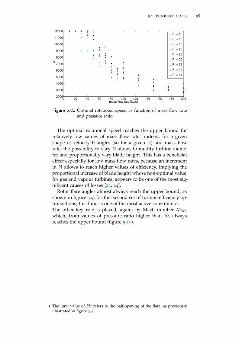
5.1 turbine maps 58
0 20 40 60 80 100 120 140 160 180 2002000
3000
4000
5000
6000
7000
8000
9000
10000
11000
12000
mass flow rate [kg/s]
N
Pr = 5
Pr = 10
Pr = 15
Pr = 20
Pr = 25
Pr = 30
Pr = 35
Pr = 40
Pr = 44
Figure 5.8.: Optimal rotational speed as function of mass flow rateand pressure ratio.
The optimal rotational speed reaches the upper bound forrelatively low values of mass flow rate: indeed, for a givenshape of velocity triangles (so for a given U) and mass flowrate, the possibility to vary N allows to modify turbine diame-ter and proportionally vary blade height. This has a beneficialeffect especially for low mass flow rates, because an incrementin N allows to reach higher values of efficiency, implying theproportional increase of blade height whose non-optimal value,for gas and vapour turbines, appears to be one of the most sig-nificant causes of losses [23, 24].
Rotor flare angles almost always reach the upper bound, asshown in figure 5.9; for this second set of turbine efficiency op-timizations, this limit is one of the most active constraints1.The other key role is played, again, by Mach number MW3
which, from values of pressure ratio higher than 10, alwaysreaches the upper bound (figure 5.10).
1 The limit value of 25° refers to the half-opening of the flare, as previouslyillustrated in figure 3.4.

5.1 turbine maps 59
0 20 40 60 80 100 120 140 160 180 2000
5
10
15
20
25
mass flow rate [kg/s]
fla
re a
ng
le r
oto
r [°
]
Pr = 5
Pr = 10
Pr = 15
Pr = 20
Pr = 25
Pr = 30
Pr = 35
Pr = 40
Pr = 44
Figure 5.9.: Flare angles for optimal design geometries, as a functionof mass flow rate and pressure ratio.
0 20 40 60 80 100 120 140 160 180 2001
1.05
1.1
1.15
1.2
1.25
1.3
1.35
1.4
mass flow rate [kg/s]
Mw
3
Pr = 5
Pr = 10
Pr = 15
Pr = 20
Pr = 25
Pr = 30
Pr = 35
Pr = 40
Pr = 44
Figure 5.10.: Values of MW3 for optimal design geometries, as afunction of mass flow rate and pressure ratio.

5.2 cycle tests 60
5.2 cycle tests
The obtained results are presented and compared in charts show-ing the most important trends as a function of pressure ratioPr = P6/P7: in fact, considering that our attention is restrictedto the cases where both T6 and the two ∆Tpp are fixed, thisparameter results to be the only active one in terms of ther-modynamic cycle configuration. The following charts mark thedifference in final power output between the two different waysof accounting for turbine efficiency. It is worth noting that, forthis particular fluid and level of heat source, the pinch point ofprimary heat exchanger is always located at recuperator outlet.
Figure 5.11.: Power output for three different values of constantturbine efficiency, in comparison with the computed-efficiency curve.
The chart in figure 5.11 shows the power output for threeassumed levels of turbine efficiency in comparison with the val-ues obtained computing expander performance. The trend ofefficiency is reported later, in figure 5.15.In this present case of study, the most restrictive constraint, interms of cycle design, is the minimum outlet temperature of ex-hausted gas TD: when imposing a maximum value of T6 consis-tently smaller than the inlet temperature of heat source (morethan 100 ◦C, as reported in figures 5.17 and 5.18), for the fixedvalue of ∆Tpp, the outlet gas temperature decreases with a steepslope and, for a fixed value of T6, the higher the pressure ratio,the lower the amount of heat available in the recuperator.Moreover, if the value of T6 is decreased, the amount of qrecalso decreases progressively. So, for the used value of T6, thetemperature TD decreases rapidly, and there is a limit value
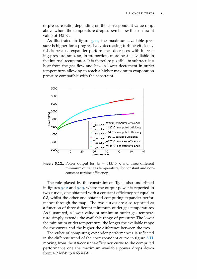
5.2 cycle tests 61
of pressure ratio, depending on the correspondent value of ηt,above whom the temperature drops down below the constraintvalue of 145 ◦C.
As illustrated in figure 5.11, the maximum available pres-sure is higher for a progressively decreasing turbine efficiency:this is because expander performance decreases with increas-ing pressure ratio, so, in proportion, more heat is available inthe internal recuperator. It is therefore possible to subtract lessheat from the gas flow and have a lower decrement in outlettemperature, allowing to reach a higher maximum evaporationpressure compatible with the constraint.
Figure 5.12.: Power output for T6 = 513.15 K and three differentminimum outlet gas temperature, for constant and non-constant turbine efficiency.
The role played by the constraint on TD is also underlinedin figures 5.12 and 5.13, where the output power is reported intwo curves, one obtained with a constant-efficiency set equal to0.8, whilst the other one obtained computing expander perfor-mance through the map. The two curves are also reported asa function of three different minimum outlet gas temperatures.As illustrated, a lower value of minimum outlet gas tempera-ture simply extends the available range of pressure: The lowerthe minimum outlet temperature, the longer the available rangefor the curves and the higher the difference between the two.
The effect of computing expander performances is reflectedin the different trend of the correspondent curve in figure 5.11:moving from the 0.8-constant-efficiency curve to the computedperformance one the maximum available power drops downfrom 4.9 MW to 4.65 MW.

5.2 cycle tests 62
Figure 5.13.: Curves for three minimum values of TD and T6 =
513.15K, for constant and non-constant turbine effi-ciency.
Figure 5.14.: Power output for three different values of constantturbine efficiency in comparison with the computed-efficiency curve (no constraint on minimum outlet gastemperature).

5.2 cycle tests 63
Figure 5.14 shows the same chart without the constraint onexit gas temperature; for a hypothetical minimum value of50 ◦C (never reached, however, as shown in figures 5.13 and5.16) the maximum power output drops down approximatelyfrom 6.321 MW to 5.365 MW.
The plot in figure 5.14 gives a more comprehensive globalvision: irrespective of the assumed value of ηt, none on theconstant-efficiency curves represents well the whole trend ofthe computed-efficiency one (black curve); this is due to theprogressive decrement of expander performance with increas-ing pressure ratio, reported in figure 5.15.
Figure 5.15.: Computed turbine efficiency in comparison with threeconstant values (no constraint on minimum outlet gastemperature).
The computed value of ηt progressively decreases from 0.7826to 0.67, crossing the horizontal lines of constant efficiency. Thecrossed points correspond to the values of pressure ratio forwhich ηt coincides with the assumed constant value.
The outlet gas temperature chart (figure 5.16) shows an in-verse trend: considering that, for a given TIT and pressure ratio,the higher the expander performance, the lower the exploitableheat in the recuperator (so the lower the outlet gas tempera-ture), the slope of the computed-turbine efficiency curve pro-gressively decreases, accounting for the increasing recoverableheat at turbine outlet.
As reported, in the most general case the limit on power is themaximum available pressure ratio. This means that a furtherincrement in electric output could be achievable increasing theevaporation pressure even more. However, the power curve in
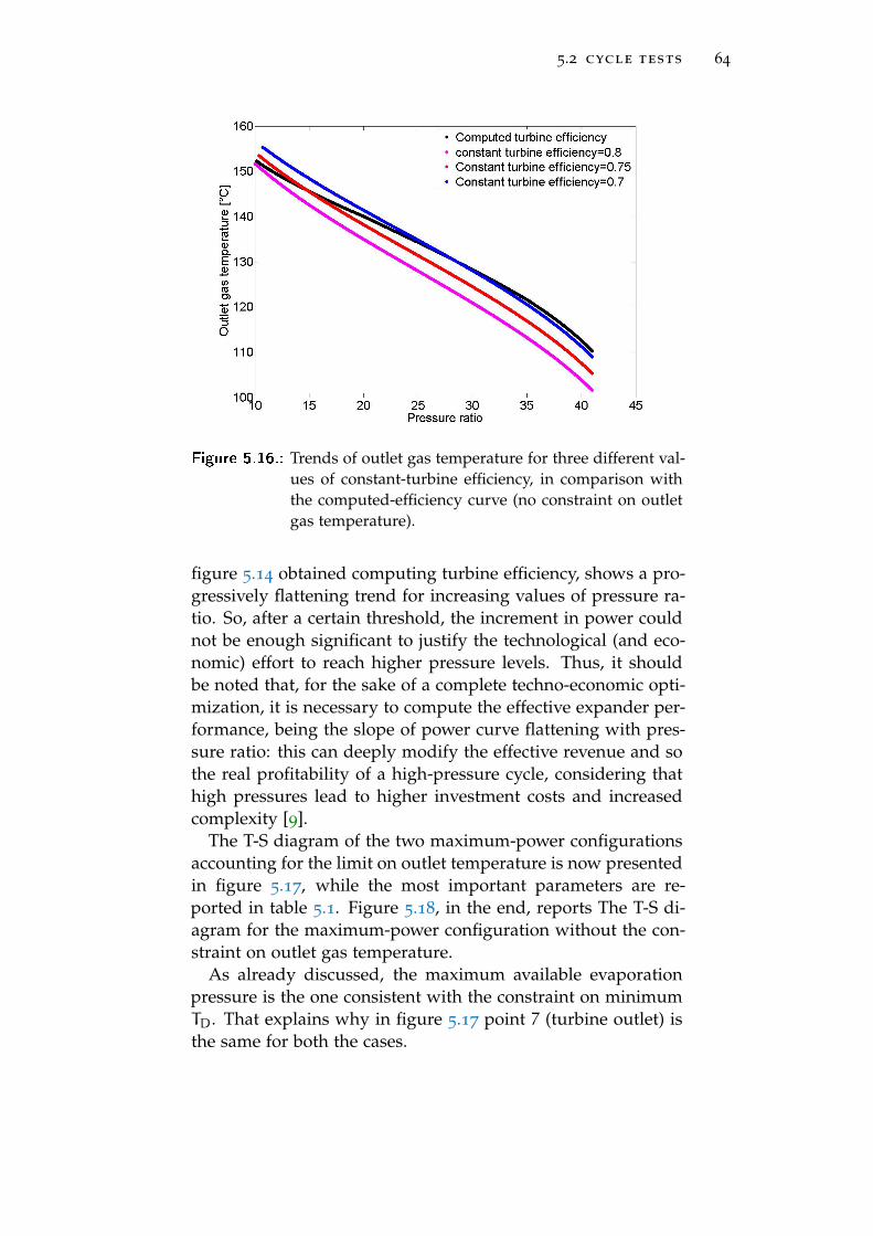
5.2 cycle tests 64
Figure 5.16.: Trends of outlet gas temperature for three different val-ues of constant-turbine efficiency, in comparison withthe computed-efficiency curve (no constraint on outletgas temperature).
figure 5.14 obtained computing turbine efficiency, shows a pro-gressively flattening trend for increasing values of pressure ra-tio. So, after a certain threshold, the increment in power couldnot be enough significant to justify the technological (and eco-nomic) effort to reach higher pressure levels. Thus, it shouldbe noted that, for the sake of a complete techno-economic opti-mization, it is necessary to compute the effective expander per-formance, being the slope of power curve flattening with pres-sure ratio: this can deeply modify the effective revenue and sothe real profitability of a high-pressure cycle, considering thathigh pressures lead to higher investment costs and increasedcomplexity [9].
The T-S diagram of the two maximum-power configurationsaccounting for the limit on outlet temperature is now presentedin figure 5.17, while the most important parameters are re-ported in table 5.1. Figure 5.18, in the end, reports The T-S di-agram for the maximum-power configuration without the con-straint on outlet gas temperature.
As already discussed, the maximum available evaporationpressure is the one consistent with the constraint on minimumTD. That explains why in figure 5.17 point 7 (turbine outlet) isthe same for both the cases.

5.2 cycle tests 65
Figure 5.17.: T-S diagram for the two maximum-power configura-tions for both the computed and constant turbine-efficiency case (blue and black, respectively).
Table 5.1.: Cycle parameters for the two maximum-power configura-tions, with constant and computed turbine efficiency.
Parameter Unit ηt = 0.8 computed ηt
Wel MW 4.881 4.711P6 bar 13.54 15.9T6 K 513.15 513.15TD
◦C 145 145
ηORC − 0.2056 0.198ηt − 0.8 0.7346mORC kg/s 45.64 46.054

5.2 cycle tests 66
Figure 5.18.: T-S diagram for the two maximum-power configura-tions for both constant and computed turbine efficiencycases (black and blue, respectively), with no constrainton outlet gas temperature.
Figure 5.19.: Output power for three different constant-turbine effi-ciencies, computed expander performances and poly-tropic efficiency.
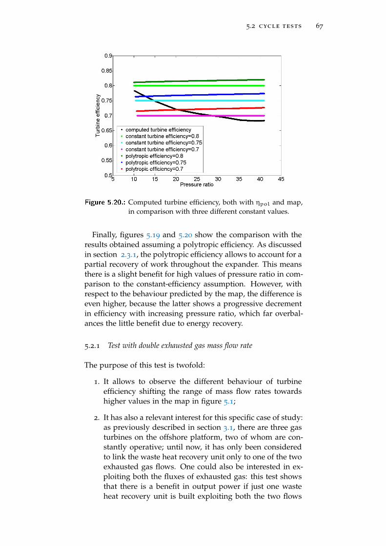
5.2 cycle tests 67
Figure 5.20.: Computed turbine efficiency, both with ηpol and map,in comparison with three different constant values.
Finally, figures 5.19 and 5.20 show the comparison with theresults obtained assuming a polytropic efficiency. As discussedin section 2.3.1, the polytropic efficiency allows to account for apartial recovery of work throughout the expander. This meansthere is a slight benefit for high values of pressure ratio in com-parison to the constant-efficiency assumption. However, withrespect to the behaviour predicted by the map, the difference iseven higher, because the latter shows a progressive decrementin efficiency with increasing pressure ratio, which far overbal-ances the little benefit due to energy recovery.
5.2.1 Test with double exhausted gas mass flow rate
The purpose of this test is twofold:
1. It allows to observe the different behaviour of turbineefficiency shifting the range of mass flow rates towardshigher values in the map in figure 5.1;
2. It has also a relevant interest for this specific case of study:as previously described in section 3.1, there are three gasturbines on the offshore platform, two of whom are con-stantly operative; until now, it has only been consideredto link the waste heat recovery unit only to one of the twoexhausted gas flows. One could also be interested in ex-ploiting both the fluxes of exhausted gas: this test showsthat there is a benefit in output power if just one wasteheat recovery unit is built exploiting both the two flows
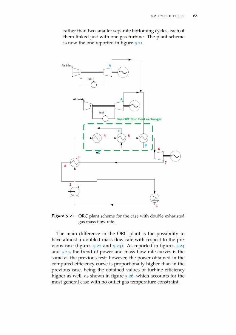
5.2 cycle tests 68
rather than two smaller separate bottoming cycles, each ofthem linked just with one gas turbine. The plant schemeis now the one reported in figure 5.21.
Figure 5.21.: ORC plant scheme for the case with double exhaustedgas mass flow rate.
The main difference in the ORC plant is the possibility tohave almost a doubled mass flow rate with respect to the pre-vious case (figures 5.22 and 5.23). As reported in figures 5.24
and 5.25, the trend of power and mass flow rate curves is thesame as the previous test: however, the power obtained in thecomputed-efficiency curve is proportionally higher than in theprevious case, being the obtained values of turbine efficiencyhigher as well, as shown in figure 5.26, which accounts for themost general case with no outlet gas temperature constraint.
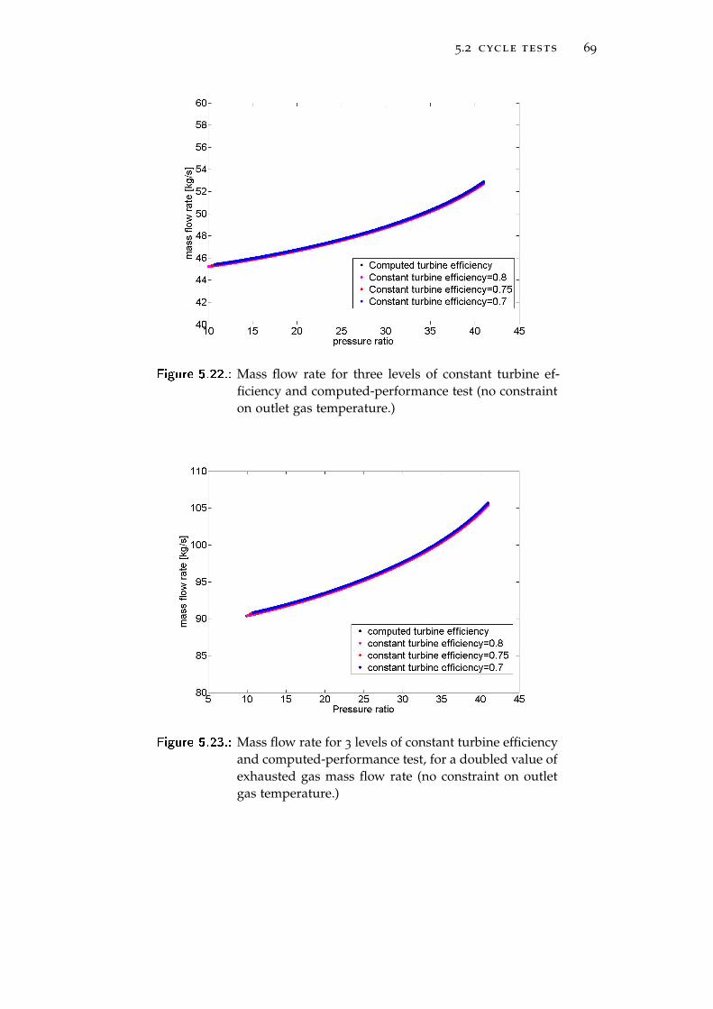
5.2 cycle tests 69
Figure 5.22.: Mass flow rate for three levels of constant turbine ef-ficiency and computed-performance test (no constrainton outlet gas temperature.)
Figure 5.23.: Mass flow rate for 3 levels of constant turbine efficiencyand computed-performance test, for a doubled value ofexhausted gas mass flow rate (no constraint on outletgas temperature.)
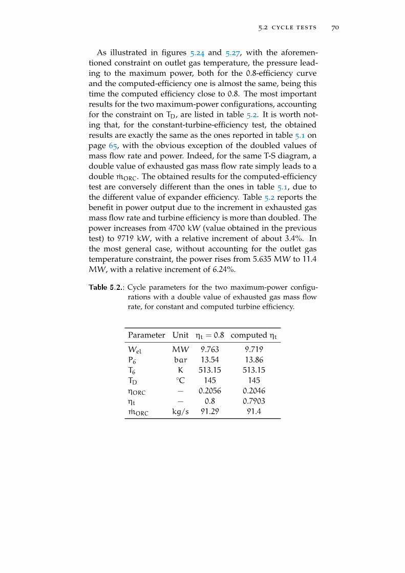
5.2 cycle tests 70
As illustrated in figures 5.24 and 5.27, with the aforemen-tioned constraint on outlet gas temperature, the pressure lead-ing to the maximum power, both for the 0.8-efficiency curveand the computed-efficiency one is almost the same, being thistime the computed efficiency close to 0.8. The most importantresults for the two maximum-power configurations, accountingfor the constraint on TD, are listed in table 5.2. It is worth not-ing that, for the constant-turbine-efficiency test, the obtainedresults are exactly the same as the ones reported in table 5.1 onpage 65, with the obvious exception of the doubled values ofmass flow rate and power. Indeed, for the same T-S diagram, adouble value of exhausted gas mass flow rate simply leads to adouble mORC. The obtained results for the computed-efficiencytest are conversely different than the ones in table 5.1, due tothe different value of expander efficiency. Table 5.2 reports thebenefit in power output due to the increment in exhausted gasmass flow rate and turbine efficiency is more than doubled. Thepower increases from 4700 kW (value obtained in the previoustest) to 9719 kW, with a relative increment of about 3.4%. Inthe most general case, without accounting for the outlet gastemperature constraint, the power rises from 5.635 MW to 11.4MW, with a relative increment of 6.24%.
Table 5.2.: Cycle parameters for the two maximum-power configu-rations with a double value of exhausted gas mass flowrate, for constant and computed turbine efficiency.
Parameter Unit ηt = 0.8 computed ηt
Wel MW 9.763 9.719P6 bar 13.54 13.86T6 K 513.15 513.15TD
◦C 145 145
ηORC − 0.2056 0.2046ηt − 0.8 0.7903mORC kg/s 91.29 91.4

5.2 cycle tests 71
Figure 5.24.: Power output for three levels of constant turbine ef-ficiency and computed-efficiency test, for a doubledvalue of exhausted gas mass flow rate.
Figure 5.25.: Power output for three levels of constant turbine effi-ciency and computed-efficiency test, with no constrainton outlet gas temperature.

5.2 cycle tests 72
Figure 5.26.: Three levels of constant turbine efficiency in compari-son with the computed-efficiency curve (no constrainton outlet gas temperature).
Figure 5.27.: T-S diagram for the two maximum-power configura-tions with constant and computed turbine efficiency(double exhausted gas mass flow rate).
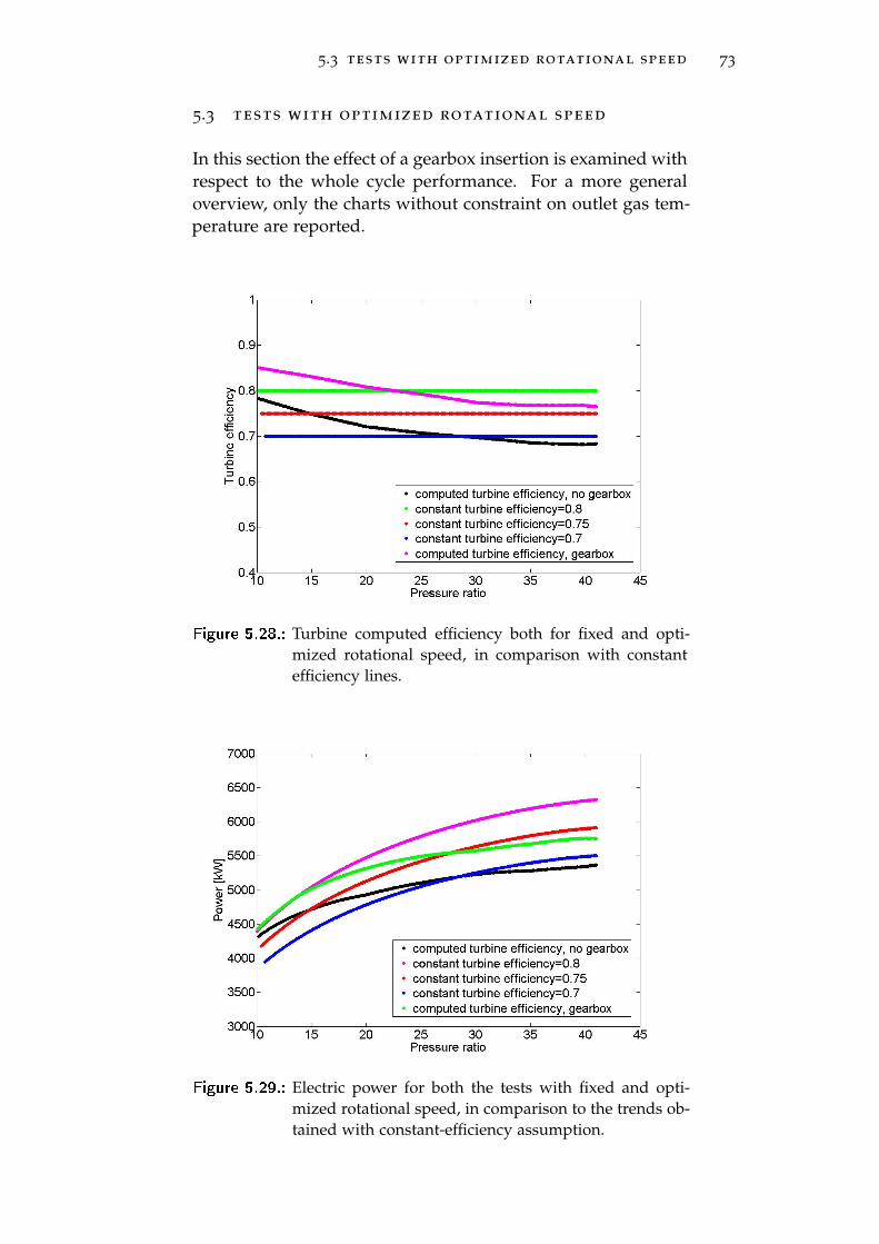
5.3 tests with optimized rotational speed 73
5.3 tests with optimized rotational speed
In this section the effect of a gearbox insertion is examined withrespect to the whole cycle performance. For a more generaloverview, only the charts without constraint on outlet gas tem-perature are reported.
Figure 5.28.: Turbine computed efficiency both for fixed and opti-mized rotational speed, in comparison with constantefficiency lines.
Figure 5.29.: Electric power for both the tests with fixed and opti-mized rotational speed, in comparison to the trends ob-tained with constant-efficiency assumption.

5.3 tests with optimized rotational speed 74
As reported in figure 5.28, the new degree of freedom allowsto achieve a higher turbine efficiency, leading to a benefit ofabout 500 kW in comparison with the case where rotationalspeed is fixed to 3000 rpm (figure 5.29). This is because, asalready shown in figure 5.8, the optimal value of rotationalspeed, in the range of mass flow rate of interest, appears tobe significantly different from 3000 rpm. The trend of the twocomputed-efficiency curves is similar:
• Both of them cross the power curves obtained with a “con-stant efficiency” assumption, showing that a map is nec-essary for both the cases to account for real expander per-formance in the whole possible range of solutions;
• both of them tend to flatten after a pressure ratio of about30, making the effort to reach more severe cycle operatingconditions of questionable effectiveness.
Figure 5.30.: Cycle electric power for three different values of gear-box efficiency.
Some comments are also necessary about gearbox efficiency.In figures 5.28 and 5.29 a value of ηgear = 0.96 has been usedto account for losses in mechanical transmission: the gearboxis not, indeed, an ideal component and its efficiency could playan important role in final power output; the chart in figure 5.30
shows the generated power for three different values of gear-box efficiency. As illustrated, even with a better expander per-formance, a value of ηgear below 0.9 invalidates the benefit ofits insertion with respect to the curve for fixed rotational speed.This analysis is also important considering that detailed infor-mation about weight, cost and efficiency of gearboxes are not
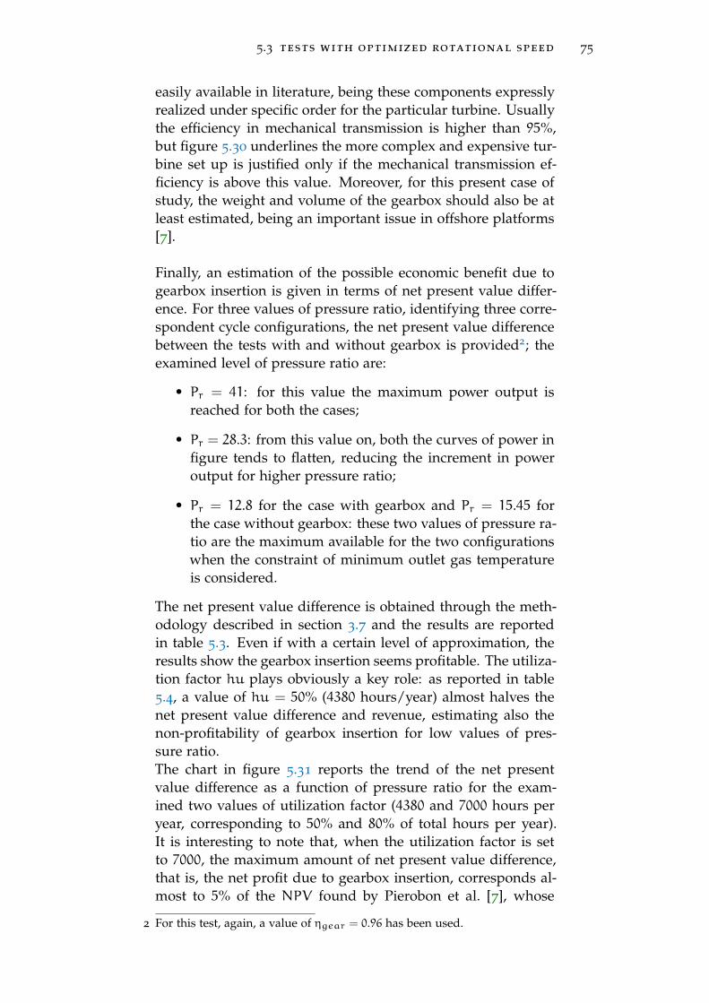
5.3 tests with optimized rotational speed 75
easily available in literature, being these components expresslyrealized under specific order for the particular turbine. Usuallythe efficiency in mechanical transmission is higher than 95%,but figure 5.30 underlines the more complex and expensive tur-bine set up is justified only if the mechanical transmission ef-ficiency is above this value. Moreover, for this present case ofstudy, the weight and volume of the gearbox should also be atleast estimated, being an important issue in offshore platforms[7].
Finally, an estimation of the possible economic benefit due togearbox insertion is given in terms of net present value differ-ence. For three values of pressure ratio, identifying three corre-spondent cycle configurations, the net present value differencebetween the tests with and without gearbox is provided2; theexamined level of pressure ratio are:
• Pr = 41: for this value the maximum power output isreached for both the cases;
• Pr = 28.3: from this value on, both the curves of power infigure tends to flatten, reducing the increment in poweroutput for higher pressure ratio;
• Pr = 12.8 for the case with gearbox and Pr = 15.45 forthe case without gearbox: these two values of pressure ra-tio are the maximum available for the two configurationswhen the constraint of minimum outlet gas temperatureis considered.
The net present value difference is obtained through the meth-odology described in section 3.7 and the results are reportedin table 5.3. Even if with a certain level of approximation, theresults show the gearbox insertion seems profitable. The utiliza-tion factor hu plays obviously a key role: as reported in table5.4, a value of hu = 50% (4380 hours/year) almost halves thenet present value difference and revenue, estimating also thenon-profitability of gearbox insertion for low values of pres-sure ratio.The chart in figure 5.31 reports the trend of the net presentvalue difference as a function of pressure ratio for the exam-ined two values of utilization factor (4380 and 7000 hours peryear, corresponding to 50% and 80% of total hours per year).It is interesting to note that, when the utilization factor is setto 7000, the maximum amount of net present value difference,that is, the net profit due to gearbox insertion, corresponds al-most to 5% of the NPV found by Pierobon et al. [7], whose
2 For this test, again, a value of ηgear = 0.96 has been used.
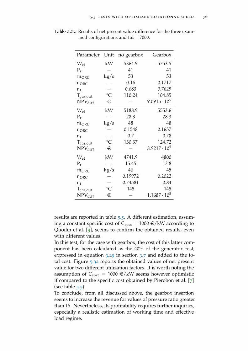
5.3 tests with optimized rotational speed 76
Table 5.3.: Results of net present value difference for the three exam-ined configurations and hu = 7000.
Parameter Unit no gearbox Gearbox
Wel kW 5364.9 5753.5Pr − 41 41
mORC kg/s 53 53
ηORC − 0.16 0.1717ηt − 0.683 0.7629Tgas,out
◦C 110.24 104.85NPVdiff e − 9.0915 · 105
Wel kW 5188.9 5553.6Pr − 28.3 28.3mORC kg/s 48 48
ηORC − 0.1548 0.1657ηt − 0.7 0.78Tgas,out
◦C 130.37 124.72NPVdiff e − 8.9217 · 105
Wel kW 4741.9 4800
Pr − 15.45 12.8mORC kg/s 46 45
ηORC − 0.19972 0.2022ηt − 0.74581 0.84Tgas,out
◦C 145 145
NPVdiff e − 1.1687 · 105
results are reported in table 5.5. A different estimation, assum-ing a constant specific cost of Cspec = 1000 e/kW according toQuoilin et al. [9], seems to confirm the obtained results, evenwith different values.In this test, for the case with gearbox, the cost of this latter com-ponent has been calculated as the 40% of the generator cost,expressed in equation 3.29 in section 3.7 and added to the to-tal cost. Figure 5.32 reports the obtained values of net presentvalue for two different utilization factors. It is worth noting theassumption of Cspec = 1000 e/kW seems however optimisticif compared to the specific cost obtained by Pierobon et al. [7](see table 5.5).To conclude, from all discussed above, the gearbox insertionseems to increase the revenue for values of pressure ratio greaterthan 15. Nevertheless, its profitability requires further inquiries,especially a realistic estimation of working time and effectiveload regime.

5.3 tests with optimized rotational speed 77
Table 5.4.: Results of net present value difference for the three exam-ined configurations and hu = 4380.
Parameter Unit no gearbox Gearbox
Wel KW 5364.9 5753.5Pr − 41 41
mORC kg/s 52, 894 52, 751ηORC − 0.16 0.1717ηt − 0.683 0.7629Tgas,out
◦C 110.24 104.85NPVdiff e − 4.018 · 105
Wel KW 5188.9 5553.6Pr − 28.3 28.3mORC kg/s 48, 422 48, 322ηORC − 0.1548 0.1657ηt − 0.7 0.78Tgas,out
◦C 130.37 124.72NPVdiff e − 4.2146 · 105
Wel KW 4741.9 4800
Pr − 15.45 12.8mORC kg/s 45, 974 45, 323ηORC − 0.19972 0.2022ηt − 0.74581 0.84Tgas,out
◦C 145 145
NPVdiff e − −1.2 · 105
Table 5.5.: Estimated total investment cost and net present value forthe case of study, Pierobon et al. [7].
Parameter Unit Value
Output power MW 6.43NPV M$ 20.1hu hours/year 7000
conv. Factor [43] $/e 0.7936Total investment cost Me 10.95247Specific cost e/kW 1703
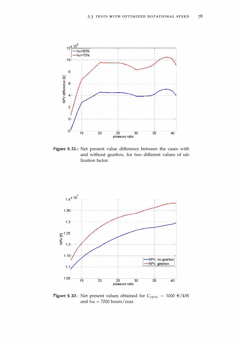
5.3 tests with optimized rotational speed 78
Figure 5.31.: Net present value difference between the cases withand without gearbox, for two different values of uti-lization factor.
Figure 5.32.: Net present values obtained for Cspec = 1000 e/kWand hu = 7000 hours/year.
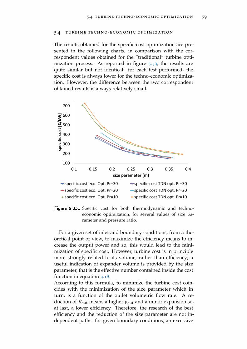
5.4 turbine techno-economic optimization 79
5.4 turbine techno-economic optimization
The results obtained for the specific-cost optimization are pre-sented in the following charts, in comparison with the cor-respondent values obtained for the “traditional” turbine opti-mization process. As reported in figure 5.33, the results arequite similar but not identical: for each test performed, thespecific cost is always lower for the techno-economic optimiza-tion. However, the difference between the two correspondentobtained results is always relatively small.
100
200
300
400
500
600
700
0.1 0.15 0.2 0.25 0.3 0.35 0.4
spe
cifi
c co
st [€
/kW
]
size parameter (m)
specific cost eco. Opt. Pr=30 specific cost TDN opt. Pr=30
specific cost eco. Opt. Pr=20 specific cost TDN opt. Pr=20
specific cost eco. Opt. Pr=10 specific cost TDN opt. Pr=10
Figure 5.33.: Specific cost for both thermodynamic and techno-economic optimization, for several values of size pa-rameter and pressure ratio.
For a given set of inlet and boundary conditions, from a the-oretical point of view, to maximize the efficiency means to in-crease the output power and so, this would lead to the mini-mization of specific cost. However, turbine cost is in principlemore strongly related to its volume, rather than efficiency; auseful indication of expander volume is provided by the sizeparameter, that is the effective number contained inside the costfunction in equation 3.18.According to this formula, to minimize the turbine cost coin-cides with the minimization of the size parameter which inturn, is a function of the outlet volumetric flow rate. A re-duction of Vout means a higher ρout and a minor expansion so,at last, a lower efficiency. Therefore, the research of the bestefficiency and the reduction of the size parameter are not in-dependent paths: for given boundary conditions, an excessive
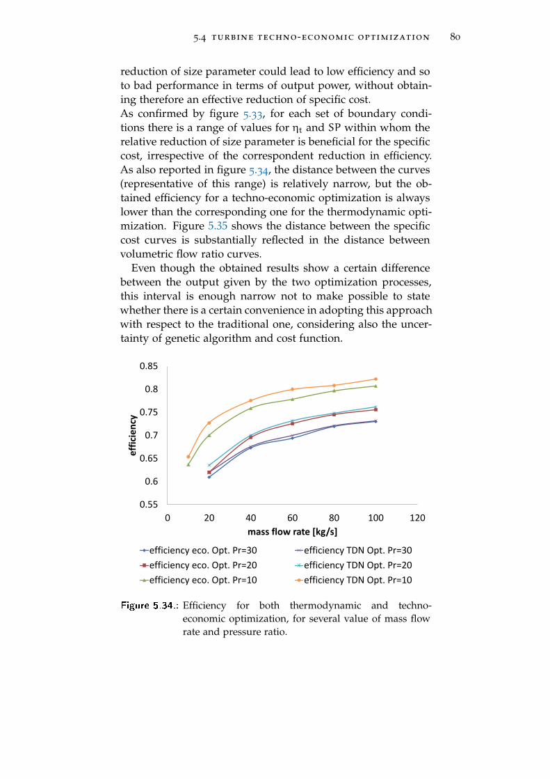
5.4 turbine techno-economic optimization 80
reduction of size parameter could lead to low efficiency and soto bad performance in terms of output power, without obtain-ing therefore an effective reduction of specific cost.As confirmed by figure 5.33, for each set of boundary condi-tions there is a range of values for ηt and SP within whom therelative reduction of size parameter is beneficial for the specificcost, irrespective of the correspondent reduction in efficiency.As also reported in figure 5.34, the distance between the curves(representative of this range) is relatively narrow, but the ob-tained efficiency for a techno-economic optimization is alwayslower than the corresponding one for the thermodynamic opti-mization. Figure 5.35 shows the distance between the specificcost curves is substantially reflected in the distance betweenvolumetric flow ratio curves.
Even though the obtained results show a certain differencebetween the output given by the two optimization processes,this interval is enough narrow not to make possible to statewhether there is a certain convenience in adopting this approachwith respect to the traditional one, considering also the uncer-tainty of genetic algorithm and cost function.
0.55
0.6
0.65
0.7
0.75
0.8
0.85
0 20 40 60 80 100 120
effi
cie
ncy
mass flow rate [kg/s]
efficiency eco. Opt. Pr=30 efficiency TDN Opt. Pr=30
efficiency eco. Opt. Pr=20 efficiency TDN Opt. Pr=20
efficiency eco. Opt. Pr=10 efficiency TDN Opt. Pr=10
Figure 5.34.: Efficiency for both thermodynamic and techno-economic optimization, for several value of mass flowrate and pressure ratio.
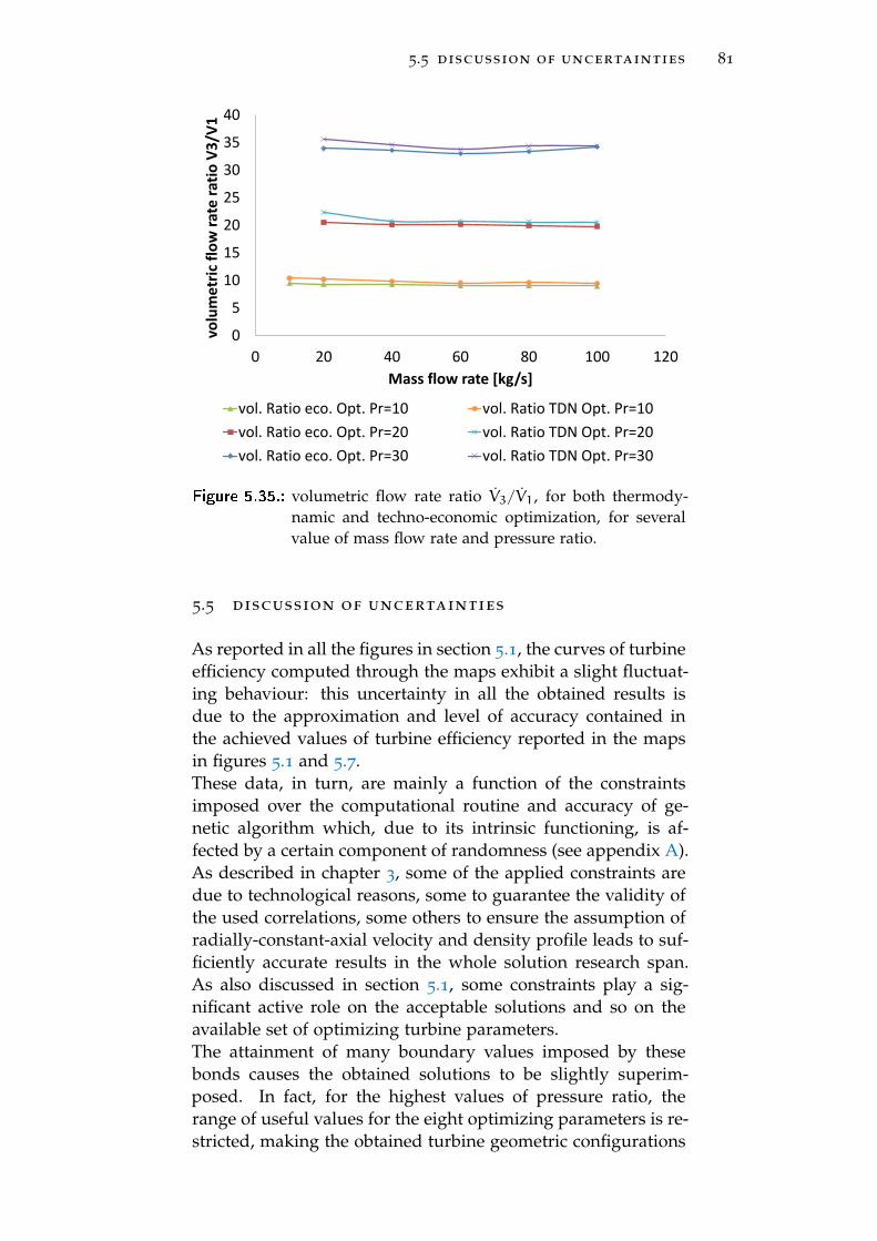
5.5 discussion of uncertainties 81
0
5
10
15
20
25
30
35
40
0 20 40 60 80 100 120
volu
me
tric
flo
w r
ate
rat
io V
3/V
1
Mass flow rate [kg/s]
vol. Ratio eco. Opt. Pr=10 vol. Ratio TDN Opt. Pr=10
vol. Ratio eco. Opt. Pr=20 vol. Ratio TDN Opt. Pr=20
vol. Ratio eco. Opt. Pr=30 vol. Ratio TDN Opt. Pr=30
Figure 5.35.: volumetric flow rate ratio V3/V1, for both thermody-namic and techno-economic optimization, for severalvalue of mass flow rate and pressure ratio.
5.5 discussion of uncertainties
As reported in all the figures in section 5.1, the curves of turbineefficiency computed through the maps exhibit a slight fluctuat-ing behaviour: this uncertainty in all the obtained results isdue to the approximation and level of accuracy contained inthe achieved values of turbine efficiency reported in the mapsin figures 5.1 and 5.7.These data, in turn, are mainly a function of the constraintsimposed over the computational routine and accuracy of ge-netic algorithm which, due to its intrinsic functioning, is af-fected by a certain component of randomness (see appendix A).As described in chapter 3, some of the applied constraints aredue to technological reasons, some to guarantee the validity ofthe used correlations, some others to ensure the assumption ofradially-constant-axial velocity and density profile leads to suf-ficiently accurate results in the whole solution research span.As also discussed in section 5.1, some constraints play a sig-nificant active role on the acceptable solutions and so on theavailable set of optimizing turbine parameters.The attainment of many boundary values imposed by thesebonds causes the obtained solutions to be slightly superim-posed. In fact, for the highest values of pressure ratio, therange of useful values for the eight optimizing parameters is re-stricted, making the obtained turbine geometric configurations
5.5 discussion of uncertainties 82
rather similar as well as, consequently, as the correspondentvalues of efficiency.
About the uncertainty related to genetic algorithm, it is worthnoting that, especially for the map with fixed rotational speed,some episodes of “numerical routine blockage” have been expe-rienced: for some combinations of mass flow rate and pressureratio, the GA got stuck around a certain value of efficiency with-out being able to produce different results, so that for somecases more than one optimization had to be performed. Forsome of them it was observed that, even with a small increasein population size and/or number of generations (see appendixA), no instability arose while for others a more consistent in-crement in both the parameters was necessary to prevent GAgetting stuck during the optimization.The first map was generated with a starting value of 550 forpopulation size and 150 generations, but for some cases thepopulation size has been risen up to 700. For the second map,in order to account for the addition of one more parameter andthe increase of possible solutions, the starting value of popula-tion size was set to 650 with 150 generations, but if launched,the second optimizations were performed with 200 generationsand a value of 800 for population size. It should be noted theoptimal value of these parameters can not be established a pri-ori: in particular, in the context of optimizing turbine design in-cluding also rotational speed, it was found that, for some cases,the same population size and number of generations lead toacceptable results in two-three days, while for others the com-putational time rose up to five-six days. For this latter cases anincrease in both the two parameters leads to higher efficienciesand reduces the computational time, while for the first ones abigger population size and generations number only increasesthe computational time with no appreciable benefit in output.
Finally, it is also worth reporting that even the possible con-tribution of the interpolating function in the turbine maps hasbeen examined: as shown from figure 5.1, many optimizationshave been performed for values of mass flow rate between 38and 54 kg/s, being this the active range of mass flow rates inthe cycle for the present case of study. However, the increase indata has not brought any appreciable difference in cycle results.
6C O N C L U S I O N S A N D P O S S I B L E F U T U R E W O R K
Here the main topics and achieved conclusion of this presentwork are reported:
• A pre-existing computational code, capable of optimizingthe geometry of a single-stage axial-flow turbine to pro-duce the best efficiency for a specific value of inlet temper-ature, mass flow rate, pressure ratio and rotational speedhas been improved and adapted to the purpose of thispresent work. The code has reported appreciable agree-ment with previous similar reliable models but some lim-its have also been identified, mainly due to its incapabilityto account for radial equilibrium effects; many constraintshave been applied in the computational routine to restrainthis effect, as well as to ensure the validity of employedcorrelations and reliability of results from both a techno-logical and thermodynamic point of view;
• The code has been integrated in a complete ORC modeland applied in the context of the Draugen offshore plat-form.Two turbine maps have been build, the first one underthe assumption of fixed rotational speed, the second oneconsidering this latter parameter among the optimizingones. Even with different values, both the maps show asimilar trend of efficiency, which increases for higher val-ues of mass flow rate and lower values of pressure ratio.For the highest amounts of this latter parameter, manythreshold values imposed by constraints, as well as manyupper and lower bounds of the optimizing parameters arereached: this causes the obtained geometries to be similarand sometimes superimposed;
• For the present case of study, the minimum value of ex-hausted gas outlet temperature appears to be the most ac-tive constraint. If this constraint is disabled, it is possibleto reach higher level of pressure with an increase in out-put power. For both these cases, the results obtained com-puting expander performance have been compared withthe ones predicted by a constant-turbine-efficiency cyclemodel; the power curves show a different trend, and nocurve based on a constant-efficiency approach can repro-duce the behaviour of the one computing expander perfor-
83

conclusions and possible future work 84
mance: for the case with fixed rotational speed, the effi-ciency progressively drops down from 0.78 to about 0.67,causing the power curve to flatten and making difficultto evaluate the real optimal configuration from a techno-economic point of view. This demonstrates a turbine mapis important for the sake of further investigations.
• The possibility of exploiting also two exhausted gas flowsfrom both the main turbines has been considered. Thissubstantially implies a double value of organic fluid massflow rate, with a benefit in produced power: due to theincrease of turbine efficiency, indeed, the final electric out-put is more than doubled;
• The optimization of rotational speed increases markedlyexpander efficiency (values below 0.75 are almost neverreached), showing an improvement in output power ofabout 500 kW in the most general case. However, theinsertion of a gearbox implies an additional cost, weightand volume. Only a very rough estimation about the costis possible and the real profitability of a gearbox insertionshould be carefully evaluated, being also weight and vol-ume an important constraint on offshore platforms. Thefirst estimation of possible revenue has been calculated asthe difference between the net present value obtained fortwo plant configurations, respectively with and withoutgearbox, showing the utilization factor plays a fundamen-tal part in the final result. The gearbox insertion seemsprofitable, but a more detailed analysis is required to es-tablish the effective convenience.
• A techno-economic optimization of the turbine has beenperformed for three levels of pressure ratio. In this pro-cess, the specific cost, instead of turbine efficiency, hasbeen chosen as the optimizing function. The obtained re-sults are very close to the ones achieved with the “classi-cal” thermodynamic optimization; however, even if thereis a range of values for size parameter among which areduction in fluid expansion (so in efficiency) leads to abenefit in specific cost, this interval is enough narrow notto make possible to state whether there is a certain con-venience in adopting this approach with respect to thetraditional one.
conclusions and possible future work 85
6.0.1 Future work
Here some suggestions for future work are given:
1. The Code structure can be improved, at least consideringthree levels of blade height to account for fluid variationsin radial direction. It would be possible to find out if thehigher computational effort is justified in terms of betterprediction of efficiency and turbine performances;
2. The off-design performance of the expander can be evalu-ated: this would be interesting, considering the request ofelectric energy in the platform is not constant and the tur-bine is likely to work in part-load regime most of time. In-deed, the analysis of turbine off-design performance canlead to a more accurate estimation of the effective rev-enue. Both the cases taking into account just one or twogas-turbine exit flows could be examined and compared;
3. A more complex cycle model accounting also for heat ex-changer dimensions (and cost) as well as turbine weightand volume can be set up. This would allow to refinethe economic analysis here performed, especially to evalu-ate the real profitability of a gearbox insertion accountingalso for eventual weight and volume constraints as wellas the aforementioned off-design considerations;
4. It would be interesting to improve the computational codein order to optimize the design of a two-stage turbine. Ithas been shown there is a maximum available pressureratio with just one stage: the implementation of a sec-ond one could increase the efficiency of the whole ex-pander, possibly making interesting also to set up a su-percritical cycle configuration; however, the higher thenumber of stages, the higher the cost, so it would beworth finding out if there is a real benefit in purchas-ing a larger and (hopefully) more efficient turbine, bothfrom a thermodynamic and economic point of view, con-sidering also weight and volume are parameters whoseimportance should not be underestimated in the contextof offshore platforms;
5. It is possible to apply the computational code also tofluid mixtures and different case of study. Previous worksshowed that there is a relevant impact in computing realturbine performances [12], but no attempt of optimizingthe whole thermodynamic cycle has been made yet;

conclusions and possible future work 86
6. The behaviour of other organic fluids, especially in termsof maximum available temperature consistent with chem-ical stability and heat source level can be examined, in thecontext of this or any other different case of study.

B I B L I O G R A P H Y
[1] L. Pantieri and T. Gordini. L’arte di scrivere con LATEX, 2009.
[2] L. Pantieri. Introduzione allo stile ClassicThesis, 2008.
[3] JabRef Development Team. JabRef, 2014. URL http://
jabref.sf.net.
[4] H.R.M. Craig and H.J.A. Cox. Performance estimation ofaxial flow turbines. Proc (Part 1), pages 407–24, 1972.
[5] Siemens. Sgt-500 gas turbine. URL http://www.
energy.siemens.com/us/en/fossil-power-generation/
gas-turbines/sgt-500.htm#content=Technical%20Data.
[6] B. Evers and P. Kötzing. Test case e/tu-4 4-stage low speedturbine. AGARD Report No. AR-275, 1990.
[7] L. Pierobon, T. Van Nguyen, U. Larsen, F. Haglind, andB. Elmegaard. Multi-objective optimization of organicrankine cycles for waste heat recovery: Application in anoffshore platform. Energy, 58:538, 2013. ISSN 03605442.
[8] A. Schuster, S. Karellas, E. Kakaras, and H. Spliethoff. En-ergetic and economic investigation of organic rankine cy-cle applications. Applied thermal engineering, 29(8):1809–1817, 2009.
[9] S. Quoilin, M. Van Den Broek, and S. Declaye. Techno-economic survey of organic rankine cycle (orc) systems. Re-newable and Sustainable Energy Reviews, 22:168, 2013. ISSN13640321, 18790690.
[10] C. Osnaghi. Teoria delle turbomacchine. Società Editrice Es-culapio, 2013.
[11] Offshore Technology. Draugen oil field, norway.URL http://www.offshore-technology.com/projects/
draugenoilfieldnorwa/.
[12] P. Gabrielli. Design and optimization of turbo-expandersfor organic rankine cycles. Master’s thesis, 2014.
[13] The mathworks®. Matlab user’s guide, 1998. URL http:
//www.mathworks.se/.
87

Bibliography 88
[14] I. H. Bell, J. Wronski, S. Quoilin, and V. Lemort. Pureand pseudo-pure fluid thermophysical property evalua-tion and the open-source thermophysical property librarycoolprop. Industrial & Engineering Chemistry Research, 53
(6):2498–2508, 2014. doi: 10.1021/ie4033999. URL http:
//pubs.acs.org/doi/abs/10.1021/ie4033999.
[15] E.W. Lemmon, M.L. Huber, and M.O. McLinden. Ref-prop, nist standard reference database 23, version 8.0. Na-tional Institute of Standards and Technology, Gaithersburg, MD,2007.
[16] Autodesk®. Autocad 2015. URL http://www.autodesk.
com/.
[17] A. Warren Adam. Organic rankine engines. Encyclopediaof Energy Technology and the Environment, 4, 1995.
[18] J. Bao and L. Zhao. A review of working fluid and ex-pander selections for organic rankine cycle. Renewable andSustainable Energy Reviews, 24:325, 2013. ISSN 13640321,18790690.
[19] M. Astolfi, M. C. Romano, and P. Bombarda. Binary ORC(organic Rankine cycles) power plants for the exploitationof medium-low temperature geothermal sources - part A:Thermodynamic optimization. Energy, 66:423, 2014. ISSN03605442.
[20] M. Astolfi, M. C. Romano, P. Bombarda, and E. Macchi. Bi-nary ORC (organic Rankine cycles) power plants for the ex-ploitation of medium-low temperature geothermal sources- part B: Techno-economic optimization. ENERGY, 66:435–446, 2014. ISSN 03605442. doi: 10.1016/j.energy.2013.11.057.
[21] D. M. Ginosar, L. M. Petkovic, and D. P. Guillen. Ther-mal stability of cyclopentane as an organic rankine cycleworking fluid. Energy & Fuels, 25(9):4138–4144, 2011.
[22] P. Klonowicz, F. Heberle, M. Preissinger, and D. Bruegge-mann. Significance of loss correlations in performance pre-diction of small scale, highly loaded turbine stages work-ing in organic rankine cycles. ENERGY, 72:322–330, 2014.ISSN 03605442. doi: 10.1016/j.energy.2014.05.040.
[23] E. Macchi. Design criteria for turbines operating with flu-ids having a low speed of sound. Von Karman Inst. for FluidDyn. Closed Cycle Gas Turbines,, 2, 1977.

Bibliography 89
[24] H. I. H. Saravanamuttoo, G. F. C. Rogers, and H. Cohen.Gas turbine theory. Pearson Education, 2001.
[25] A. Beccari. Macchine. 1993. ISBN 9788879920339.
[26] P. Kundu and I. Cohen. Fluid mechanics, 730 pp, 2000.
[27] E. Macchi and A. Perdichizzi. Efficiency prediction foraxial-flow turbines operating with nonconventional fluids.American Society of Mechanical Engineers (Paper), (81), 1981.ISSN 04021215.
[28] G. Lozza. A comparison between the craig-cox and thekacker-okapuu methods of turbine performance predic-tion. Meccanica, 17(4):211–221, 1982. ISSN 00256455,15729648. doi: 10.1007/BF02128314.
[29] L. Pierobon, F. Haglind, U. Larsen, and T. Van Nguyen.Optimization of organic rankine cycles for off-shore appli-cations. Proceedings of the ASME Turbo Expo, 5:–, 2013. doi:10.1115/GT2013-94108.
[30] Ministry of the Environment (Norway). The gov-ernment is following up on the climate agree-ment, 2012. URL http://www.regjeringen.
no/en/archive/Stoltenbergs-2nd-Government/
Ministry-of-the-Environment/
Nyheter-og-pressemeldinger/pressemeldinger/2012/
the-government-is-following-up-on-the-cl.html?id=
704137.
[31] M.E. Deich, G.A. Filippov, and L. Ya Lazarev. Atlas profileireshotok osevykh turbomachin, 1965.
[32] D. G. Ainley and G. C. R. Mathieson. An examination ofthe flow and pressure losses in blade rows of axial-flowturbines. Aeronautic research council, 1951.
[33] M.H. Vavra. Axial flow turbines. Lecture Series, 15, 1969.
[34] S.C. Kacker and U. Okapuu. A mean line predictionmethod for axial flow turbine efficiency. Journal of Engi-neering for Gas Turbines and Power, 104(1):111–119, 1982.
[35] M. Obitko. Genetic algorithms. URL http://obitko.com/
tutorials/genetic-algorithms/.
[36] A. Galliani and E. Pedrocchi. Analisi exergetica. Polipress,2006.

Bibliography 90
[37] M. Pasetti, C. M. Invernizzi, and P. Iora. Thermal sta-bility of working fluids for organic rankine cycles: Animproved survey method and experimental results forcyclopentane, isopentane and n-butane. Applied Ther-mal Engineering, 73(1):762 – 772, 2014. ISSN 1359-4311.doi: http://dx.doi.org/10.1016/j.applthermaleng.2014.08.017. URL http://www.sciencedirect.com/science/
article/pii/S1359431114006796.
[38] Wikipedia. Net present value, . URL http://en.
wikipedia.org/wiki/Net_present_value.
[39] A. Bejan and M. J. Moran. Thermal design and optimization.John Wiley & Sons, 1996.
[40] Index mundi, natural gas monthly price, September2014. URL http://www.indexmundi.com/commodities/
?commodity=natural-gas¤cy=nok.
[41] Wikipedia. British thermal unit, . URL http:
//en.wikipedia.org/wiki/British_thermal_unit#
For_natural_gas.
[42] K. Rypdal. Anthropogenic emissions of the greenhouse gasesCO2, CH4 and N2O in Norway: A documentation of methodsof estimation, activity data and emission factors. Statistisk sen-tralbyrêa (Oslo), 1993.
[43] Yahoo Finance. Money currency converter. URLhttps://it.finance.yahoo.com/valute/convertitore/
#from=EUR;to=NOK;amt=1.
[44] Politecnico di Milano. Axtur. URL http://www.energia.
polimi.it/.
[45] I. H. Johnston and L. R. Knight. Tests on a single-stageturbine comparing the performance of twisted with un-twisted rotor blades. 1953.
[46] M. Mahalakshmi, P. Kalaivani, and E.Kiruba Nesamalar. Areview on genetic algorithm and its applications. Interna-tional Journal of Computing Algorithm, 02:415–423, Novem-ber 2013.
[47] The Mathworks®. Genetic algorithm. URL http://www.
mathworks.se/discovery/genetic-algorithm.html.
AT H E G E N E T I C A L G O R I T H M
A detailed description of genetic algorithms and their theo-retical background, potential and applications is provided byObitko [35] or Mahalakshmi et al. [46].Here follows a more detailed description about the structureand working routine of genetic algorithm (GA). This descrip-tion is not exhaustive but it would provide a better comprehen-sion of the task in the context of this present work.
The structure of genetic algorithm is inspired by Darwin’s the-ory about evolution. In simple words, the solution obtained byGA is evolved during the computational process.
All living organisms are an array of cells, each one containingthe same amount of chromosomes which, in turn, are strings ofDNA and serves as a model for the whole organism. A chro-mosome is made of genes, blocks of DNA, and basically eachof them encodes a trait of the living organism, for example thecolour of skin.During reproduction, genes from parents recombine in someway (crossover) and a new set of chromosome is so created.Then, some changes in DNA element can occur, mainly due toerrors in copying genes from parents (mutation). This meansthe new set of chromosomes could be different from the purerecombinations of parental genes. The fitness of an organism ismeasured by its success in life and surviving in the surround-ing environment: organisms with higher fitness will surviveand, by their reproduction, new offspring with better geneswill arise.
The mathematical seek for a optimal solution, coincides withthe research of some extreme value (minimum or maximum)for a particular function. The space of all feasible solutions iscalled search space (also state space). Each point in the searchspace represent one acceptable solution and each of them canbe “marked” by its value or fitness for the problem.
The mathematical structure of GA basically mirrors the afore-mentioned biological mechanism: for a determined number ofchromosomes (population size) a new offspring is created re-combining genes of the existing ones. The fitness of each newchromosome is evaluated and the best of each generation iskept in memory. This process goes on until the maximum num-ber of generations is reached or no further change in the found
91
the genetic algorithm 92
maximum/minimum value for the optimizing function is ob-tained1.Thus each chromosome is a set of input value for the optimiz-ing function. The goal is to find the chromosome with the bestfitness that is, the best set of input values for a certain functionthat maximises/minimizes it.
However, the “evolution” process is rather more complicatedthan this, being the new incoming generation a product ofcrossover, mutation and randomness. The first and second arethe most important part of the genetic algorithm while the thirdis intrinsically contained in the whole process. We define:
1. Crossover probability: index of how often crossover isperformed. If this value is zero, the offspring is an exactcopy of parents. If there is a crossover, offspring is madefrom parts of parents’ chromosome. If crossover probabil-ity is 100%, all the new generation is made by crossover.If it is 0%, the new offspring is made from exact copiesof chromosomes of the population; it is worth noting thisdoes not mean that the new generation is the same as theprevious one. Crossover is made in hope that new chro-mosomes will have the best parts of old parents, forminga hopefully better generation. However it is good to letsome part of old population survive to the next genera-tion.
2. Mutation probability states how often parts of a chromo-some will be mutated. If there is no mutation, offspringis taken after crossover (or copy) without any change. Ifa component of mutation fraction exists, at least a smallpart of the chromosome is changed. If mutation probabil-ity is 100%, the whole chromosome genes are changed,if it is 0%, all of them are untouched from the previ-ous step. Mutation process could be completely randomor partially/totally governed by a particular probabilitydistribution [47]. This process is made to prevent GAgetting stuck into a specific local extreme; even though,theoretically, this problem should not often occur, accord-ing to the particular function to be optimized (namely itsnon-continuity, eventual fluctuating and non-linear trend,presence of local extremes and so on), this could be oneof the main causes of uncertainty of this method.
3. Population size: the number of chromosomes containedin a single population (or generation). If this number is
1 If no change is observed in the optimizing function within the next 50 gen-erations, the algorithm stops calculating.
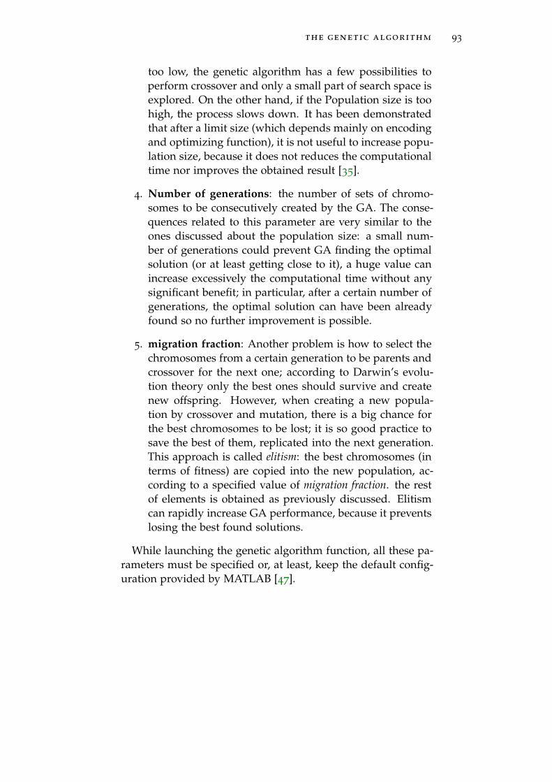
the genetic algorithm 93
too low, the genetic algorithm has a few possibilities toperform crossover and only a small part of search space isexplored. On the other hand, if the Population size is toohigh, the process slows down. It has been demonstratedthat after a limit size (which depends mainly on encodingand optimizing function), it is not useful to increase popu-lation size, because it does not reduces the computationaltime nor improves the obtained result [35].
4. Number of generations: the number of sets of chromo-somes to be consecutively created by the GA. The conse-quences related to this parameter are very similar to theones discussed about the population size: a small num-ber of generations could prevent GA finding the optimalsolution (or at least getting close to it), a huge value canincrease excessively the computational time without anysignificant benefit; in particular, after a certain number ofgenerations, the optimal solution can have been alreadyfound so no further improvement is possible.
5. migration fraction: Another problem is how to select thechromosomes from a certain generation to be parents andcrossover for the next one; according to Darwin’s evolu-tion theory only the best ones should survive and createnew offspring. However, when creating a new popula-tion by crossover and mutation, there is a big chance forthe best chromosomes to be lost; it is so good practice tosave the best of them, replicated into the next generation.This approach is called elitism: the best chromosomes (interms of fitness) are copied into the new population, ac-cording to a specified value of migration fraction. the restof elements is obtained as previously discussed. Elitismcan rapidly increase GA performance, because it preventslosing the best found solutions.
While launching the genetic algorithm function, all these pa-rameters must be specified or, at least, keep the default config-uration provided by MATLAB [47].

BTA B L E S A N D U S E F U L F I G U R E S
Figure B.1.: Figure 19 of Craig and Cox losses estimation procedure(Craig and Cox [4]).
94

tables and useful figures 95
Table B.1.: Complete list of required turbine input parameters forthe computational routine
Parameter Unit Description
Optimizing parametersα1 ° absolute nozzle inlet fluid
angleψ - ∆Htot/(u
2m/2)
(omin)n m Nozzle throat sectionor m Rotor throat sectioncn m Nozzle axial chordcr m Rotor axial chord(os )n - Blade outlet section/pitch,
nozzle(os )r - Blade outlet section/pitch,
rotor
Cycle requirementsm kg/s Mass flow rateP01 bar Total inlet pressureP03 bar Total outlet pressureN rpm Rotational speedT01 K Total inlet temperaturefluid - fluid type
Fixed inputshhh - Nozzle outlet/rotor inlet
height ratioMcd - Mach number for conv.-div.
Nozzle(te/o)n - Trailing edge thick-
ness/outlet section fornozzle
(te/o)r - Trailing edge thick-ness/outlet section forrotor
Re - Reynolds numberimin,n ° Minimum incidence value
for nozzleimin,r ° Minimum incidence value
for rotorksbr - Relative surface roughnessε m Back surface radiuscontrolled expansion - yes/noshrouded blades - yes/nooverlap m overlaptolf - Tolerance factor for conver-
gence

tables and useful figures 96
Table B.2.: Complete list of required input parameters for cyclemodel
parameter default value Unit Description
mgas 93.5 kg/s Exhausted gas massflow rate
Tgas,in 376 ◦C Inlet gas tempera-ture
Tgas,out,min 145 ◦C Minimum ex-hausted gas outlettemperature
cp,gas 1.1 kJ/(kg K) Exhausted gas spe-cific heat
ηp 0.8 - Pump efficiencyηgen 0.98 - Elecric generator ef-
ficiencyηturb 0.8 - Turbine efficiency
(only for constant-efficiency tests)
ηgear 0.96 - Gearbox efficiency(only if gearboxpresence ins consid-ered)
fluid cyclopentane - Organic fluid to beused
Pcond 1 bar Condensation pres-sure
Pr,max 0.9 · Pcrit - Maximum availablepressure ratio
∆Tpp,rec 15 ◦C Pinch point temper-ature difference ininternal recuperator
∆Tpp 10 ◦C Pinch point tem-perature differencein main heat ex-changer
TIT 513.15 K Turbine inlet tem-perature
tolf 0.01 - Tollerance factor forconvergence in tur-bine map interpola-tion
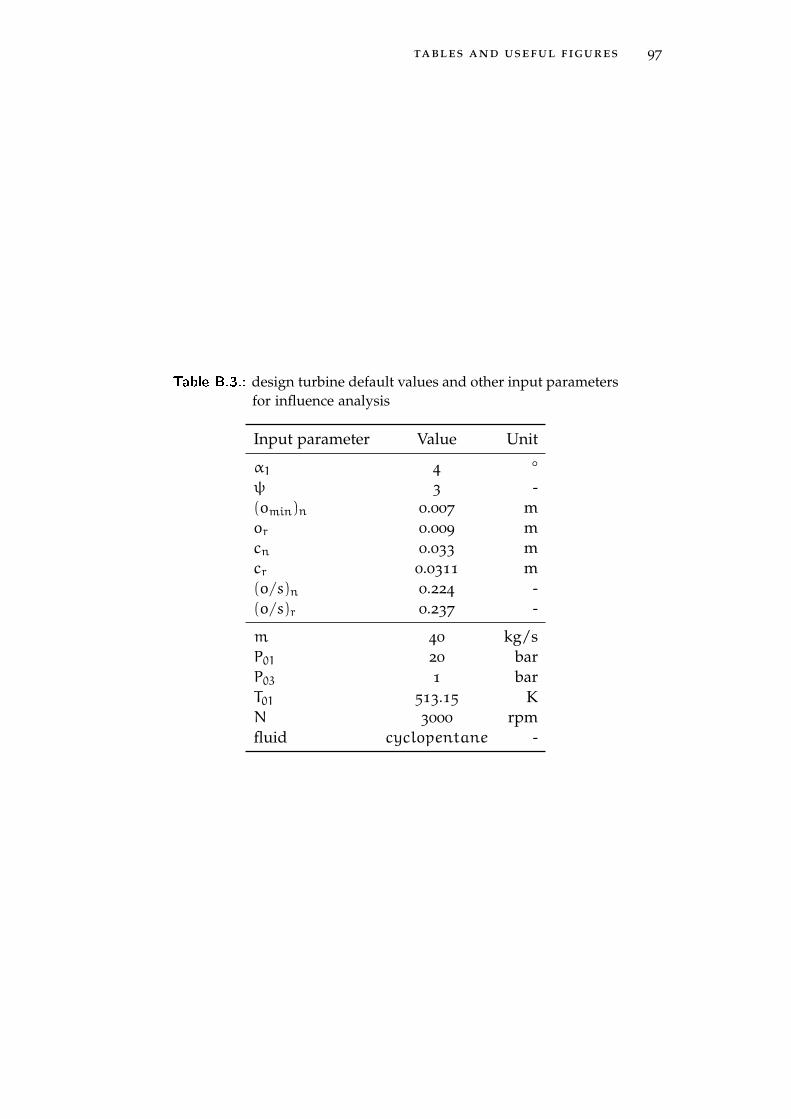
tables and useful figures 97
Table B.3.: design turbine default values and other input parametersfor influence analysis
Input parameter Value Unit
α1 4 °ψ 3 -(omin)n 0.007 mor 0.009 mcn 0.033 mcr 0.0311 m(o/s)n 0.224 -(o/s)r 0.237 -
m 40 kg/sP01 20 barP03 1 barT01 513.15 KN 3000 rpmfluid cyclopentane -
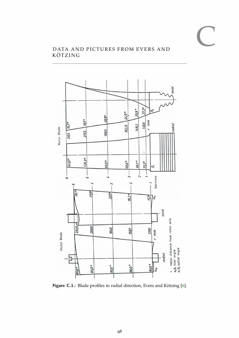
CD ATA A N D P I C T U R E S F R O M E V E R S A N DK Ö T Z I N G
Figure C.1.: Blade profiles in radial direction, Evers and Kötzing [6].
98
data and pictures from evers and kötzing 99
Figure C.2.: Blade sections in radial direction, Evers and Kötzing [6].
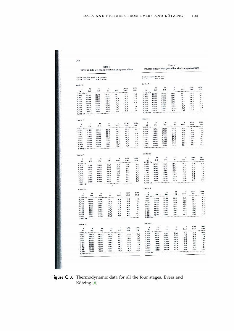
data and pictures from evers and kötzing 100
Figure C.3.: Thermodynamic data for all the four stages, Evers andKötzing [6].
Related Documents