AN INTRODUCTION TO THE FINITE ELEMENT METHOD FOR … … · C. Finite Element Method The finite element method also employs the variational form of the problem similar to the Rayleigh-Ritz

ANINTRODUCTION

TO THEFINITE

ELEMENTMETHOD

FORYOUNG

ENGINEERSBy: Eduardo DeSantiago, PhD, PE, SE

Table of Contents

SECTION I INTRODUCTION ............................................................................................ 2

SECTION II 1-D EXAMPLE ............................................................................................... 2

SECTION III DISCUSSION ............................................................................................... 13

SECTION IV REFERENCES ............................................................................................. 14

Primera An Introduction to the Finite Element Method for Young Engineers 1

I. Introduction

The finite element method (FEM) has become an indispensable modern tool for mechanical and

structural engineers. It is difficult to imagine an engineering firm that doesn’t have access to

one of the many available FEM commercial codes. Modern commercial FEM codes have become

very sophisticated and allow for the development of complex 3-D models with relative ease.

Unfortunately, the ease of use of these sophisticated codes may lead the unsuspecting user to

assume a higher level of understanding of the complex theoretical underpinnings of the finite

element method than actually exists. Leading to this situation is the fact that many engineers

graduate without ever taking a course on FEM theory, yet make use of the method on a daily

basis. Needless to say this situation is fraught with danger.

This article is the first in a series that will attempt to introduce some of the rich and complex

theory that forms the foundation of the finite element method of analysis in the hopes that it will

stir an interest in the reader to develop a more fundamental understanding of the method if it

doesn’t already exist. The ideas to be presented have been developed through several years of

graduate study, research, and teaching in finite element analysis by the author. Many of the

topics to be covered come directly from graduate courses taught on FEM at the Illinois Institute

of Technology.

II. 1-D Example

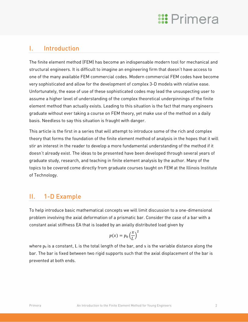
To help introduce basic mathematical concepts we will limit discussion to a one-dimensional

problem involving the axial deformation of a prismatic bar. Consider the case of a bar with a

constant axial stiffness EA that is loaded by an axially distributed load given by

𝑝𝑝(𝑥𝑥) = 𝑝𝑝0 �𝑥𝑥𝐿𝐿 �2

where p0 is a constant, L is the total length of the bar, and x is the variable distance along the

bar. The bar is fixed between two rigid supports such that the axial displacement of the bar is

prevented at both ends.


If we denote the axial displacement of the bar as u(x); then to satisfy equilibrium at every single

point along the length of the bar, the following equation must hold:

𝐸𝐸𝐸𝐸𝑑𝑑2𝑢𝑢𝑑𝑑𝑥𝑥

+ 𝑝𝑝(𝑥𝑥) = 0

The exact solution for the above equation can be shown to be:

Now one can use the above 1-D example with a known exact solution to compare and contrast

common numerical methods including the finite element method used to find approximate

solutions to the problem.

A. Finite Difference Method

In the finite difference method, approximations to the second order derivative are used to obtain

a numerical solution to the differential equation of equilibrium. In general for any function f(x) defined over a finite range one can split the range into n equal intervals each of length h. Thus:


In the “forward difference method” the first and second derivatives of the function at xi are

approximated using information at xi+1 and xi+2, thus the term “forward.” These derivatives are

given by:

𝑑𝑑𝑑𝑑(𝑥𝑥𝑖𝑖)𝑑𝑑𝑥𝑥

≈𝑑𝑑𝑖𝑖+1 − 𝑑𝑑𝑖𝑖

ℎ

𝑑𝑑2𝑑𝑑(𝑥𝑥𝑖𝑖)𝑑𝑑𝑥𝑥

≈𝑑𝑑𝑖𝑖+2 − 2𝑑𝑑𝑖𝑖+1 + 𝑑𝑑𝑖𝑖

ℎ2

In the “backward difference method” the first and second derivatives of the function at xi are

approximated using information at xi-1 and xi-2, thus the term “backward.” These derivatives are

given by:


≈𝑑𝑑𝑖𝑖 − 𝑑𝑑𝑖𝑖−1

ℎ


≈𝑑𝑑𝑖𝑖 − 2𝑑𝑑𝑖𝑖−1 + 𝑑𝑑𝑖𝑖−2

ℎ2

In the “central difference method” the first and second derivatives of the function at xi are

approximated using information at both xi-1 and xi+1, thus the term “central.” These derivatives

are given by:


≈𝑑𝑑𝑖𝑖+1 − 𝑑𝑑𝑖𝑖−1

2ℎ


≈𝑑𝑑𝑖𝑖+1 − 2𝑑𝑑𝑖𝑖 + 𝑑𝑑𝑖𝑖−1

ℎ2

Before taking a look at how these methods behave for the model 1-D problem it is important to

note that the complexity of the finite difference method approximations increases as the order

of the derivatives increases. Our relatively simple problem only has second order derivatives,

but for many physical problems the order of the highest derivative is greater than two. The

Bernouilli-Euler Beam theory, for example, leads to a differential equation of equilibrium that

contains a fourth order derivative. For a fourth order derivative, the difference method would

lead to approximations for the fourth order derivative that would contain five terms in the

numerator.


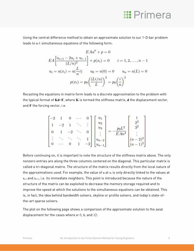
Using the central difference method to obtain an approximate solution to our 1-D bar problem

leads to n-1 simultaneous equations of the following form:

Recasting the equations in matrix form leads to a discrete approximation to the problem with

the typical format of Kd=F, where K is termed the stiffness matrix, d the displacement vector,

and F the forcing vector, i.e.

Before continuing on, it is important to note the structure of the stiffness matrix above. The only

nonzero entries are along the three columns centered on the diagonal. This particular matrix is

called a tri-diagonal matrix. The structure of the matrix results directly from the local nature of

the approximations used. For example, the value of u at xi is only directly linked to the values at

xi-1 and xi+1, i.e. its immediate neighbors. This point is introduced because the nature of the

structure of the matrix can be exploited to decrease the memory storage required and to

improve the speed at which the solutions to the simultaneous equations can be obtained. This

is, in fact, the idea behind bandwidth solvers, skyline or profile solvers, and today’s state-of-

the-art sparse solvers.

The plot on the following page shows a comparison of the approximate solution to the axial

displacement for the cases where n=3, 6, and 12:


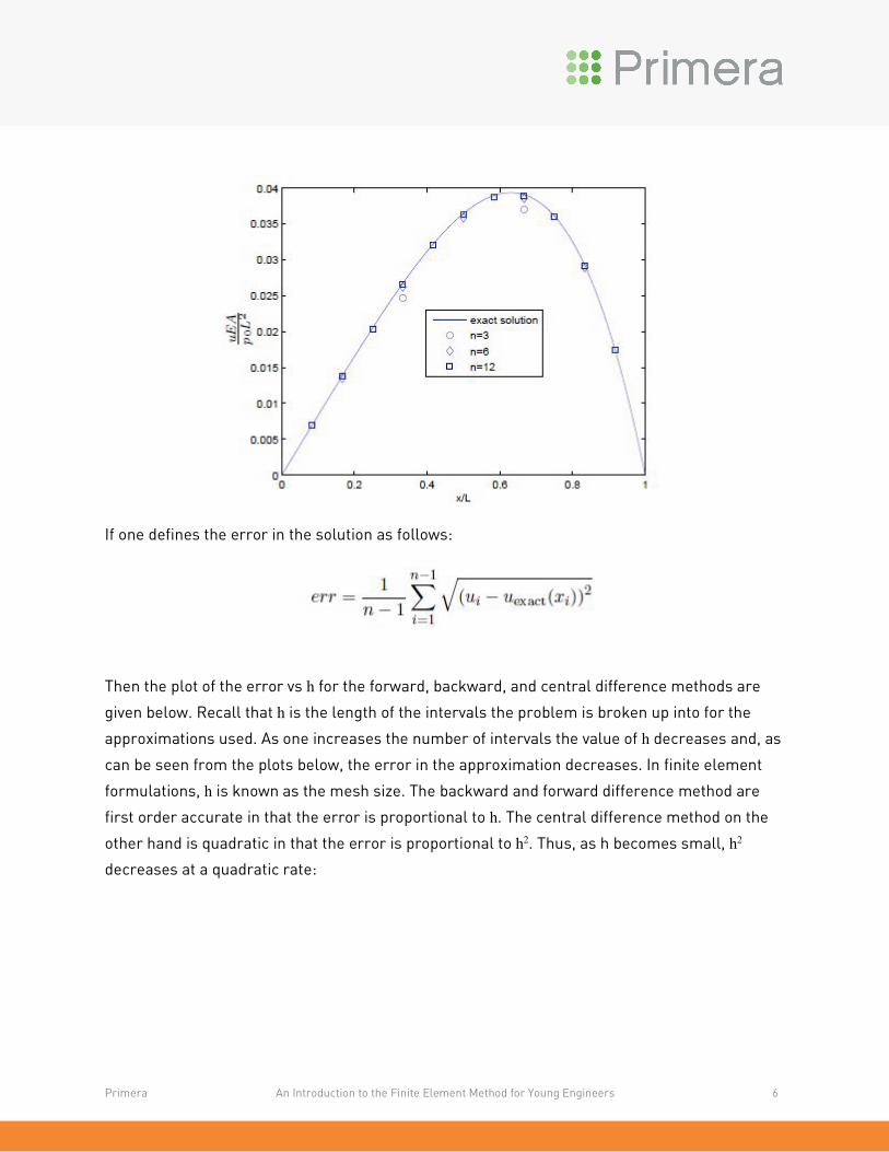
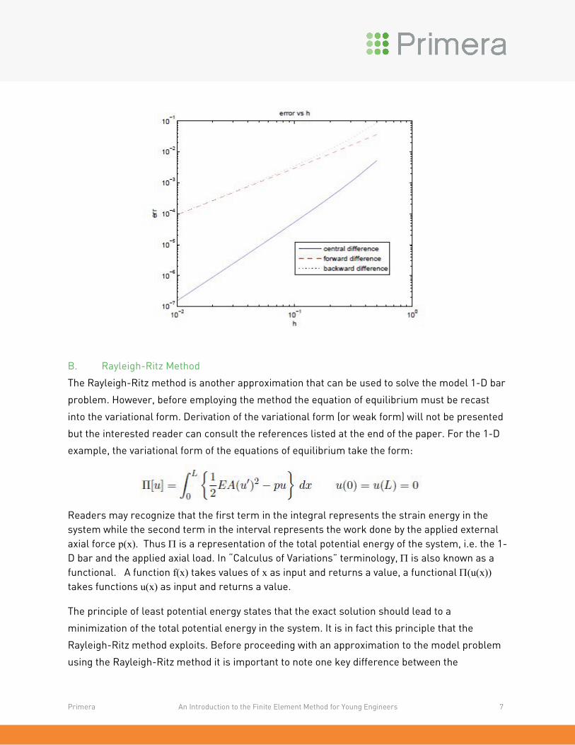
If one defines the error in the solution as follows:

Then the plot of the error vs h for the forward, backward, and central difference methods are

given below. Recall that h is the length of the intervals the problem is broken up into for the

approximations used. As one increases the number of intervals the value of h decreases and, as

can be seen from the plots below, the error in the approximation decreases. In finite element

formulations, h is known as the mesh size. The backward and forward difference method are

first order accurate in that the error is proportional to h. The central difference method on the

other hand is quadratic in that the error is proportional to h2. Thus, as h becomes small, h2

decreases at a quadratic rate:


B. Rayleigh-Ritz Method

The Rayleigh-Ritz method is another approximation that can be used to solve the model 1-D bar

problem. However, before employing the method the equation of equilibrium must be recast

into the variational form. Derivation of the variational form (or weak form) will not be presented

but the interested reader can consult the references listed at the end of the paper. For the 1-D

example, the variational form of the equations of equilibrium take the form:

Readers may recognize that the first term in the integral represents the strain energy in the system while the second term in the interval represents the work done by the applied external axial force p(x). Thus Π is a representation of the total potential energy of the system, i.e. the 1-D bar and the applied axial load. In “Calculus of Variations” terminology, Π is also known as a functional. A function f(x) takes values of x as input and returns a value, a functional Π(u(x)) takes functions u(x) as input and returns a value.

The principle of least potential energy states that the exact solution should lead to a

minimization of the total potential energy in the system. It is in fact this principle that the

Rayleigh-Ritz method exploits. Before proceeding with an approximation to the model problem

using the Rayleigh-Ritz method it is important to note one key difference between the


differential equation of equilibrium presented for the finite difference methods and the

variational form. Recall that for the differential equation of equilibrium, a second order

derivative appeared in the equation which necessitated an approximation. In the variational

form, the highest derivative is first order which one would expect would lead to a creation of

simpler approximations.

One drawback of the Rayleigh-Ritz method is the need to use global approximations therefore

the resulting stiffness matrices will be full of nonzeros. Another important consideration for the

Rayleigh-Ritz method is that the approximations used must have continuous first derivatives.

For the 1-D model problem under consideration, one needs to use approximations to the axial

displacement û(x) that are equal to zero at both x=0 and x=L. Using a quadratic approximation

of the form:

where c1 is an unknown constant, leads to a total potential energy for the system given by:

Minimizing Π(û(x)) with respect to c1 results in the following:

Here the term 1/3 EAL3 can be thought of as the 1x1 stiffness matrix, c1 as the one term

displacement vector, and –p0 L3/20 as the one term force vector. Substituting the value obtained

for c1 into our quadratic approximation for u(x) leads to the following approximation for the axial

displacement:


Similarly a two term approximation to the axial displacement can be made leading to the

following:

The following plot compares the exact solution for u(x) and the approximations to the axial

displacement obtained above using the one term and two term approximations:


C. Finite Element Method The finite element method also employs the variational form of the problem similar to the Rayleigh-Ritz method. However, the finite element method makes use of the variational form after applying the minimization of the total potential energy. Suppose u(x) is the axial displacement function that minimizes Π then inserting a function of the form u(x) + δu(x) will always lead to a larger value for the total potential energy of the system for any arbitrary function δu(x) (note that δu(x) must be equal to 0 at x=0 and x=L for the model 1-D problem). According to the Fundamental Theorem of Calculus of Variations, u(x) minimizes Π if and only if the following holds

for any function δu(x) that is zero at x=0 and x=L. The above equation represents the starting point for the finite element approximation. Readers may recognize that the above simply represents the virtual work if one considers the function δu(x) to be a virtual axial displacement with the first term representing the internal virtual work and the second term representing the external virtual work.

To obtain an approximation to our model problem we need to approximate both the axial displacement u(x) and the virtual displacement δu(x). The Galerkin formulation of the model problem makes use of the same type of approximations for both the axial displacement and the virtual axial displacement. Furthermore, a key aspect of the above formulation is that our approximations only require piecewise continuity. The first and higher order derivatives of the approximations need not be continuous throughout the problem domain. This key aspect allows the use of simple approximations for the model problem and is a key advantage of the finite element method.

Replacing u(x) and δu(x) with approximations leads to the Galerkin formulation of our model problem as follows

Similar to the finite difference method we divide the bar into intervals from xi to xi+1, i=0, 1, 2, …, n with x0=0 and xn=L; where each interval is defined as an element of finite length. Each location


of a discrete approximation, xi, is defined as a node. Together the nodes and elements of the approximation define the finite element mesh.

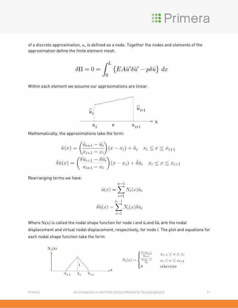
Within each element we assume our approximations are linear.

Mathematically, the approximations take the form:

Rearranging terms we have:

Where Ni(x) is called the nodal shape function for node i and ûi and δûi are the nodal

displacement and virtual nodal displacement, respectively, for node i. The plot and equations for

each nodal shape function take the form:


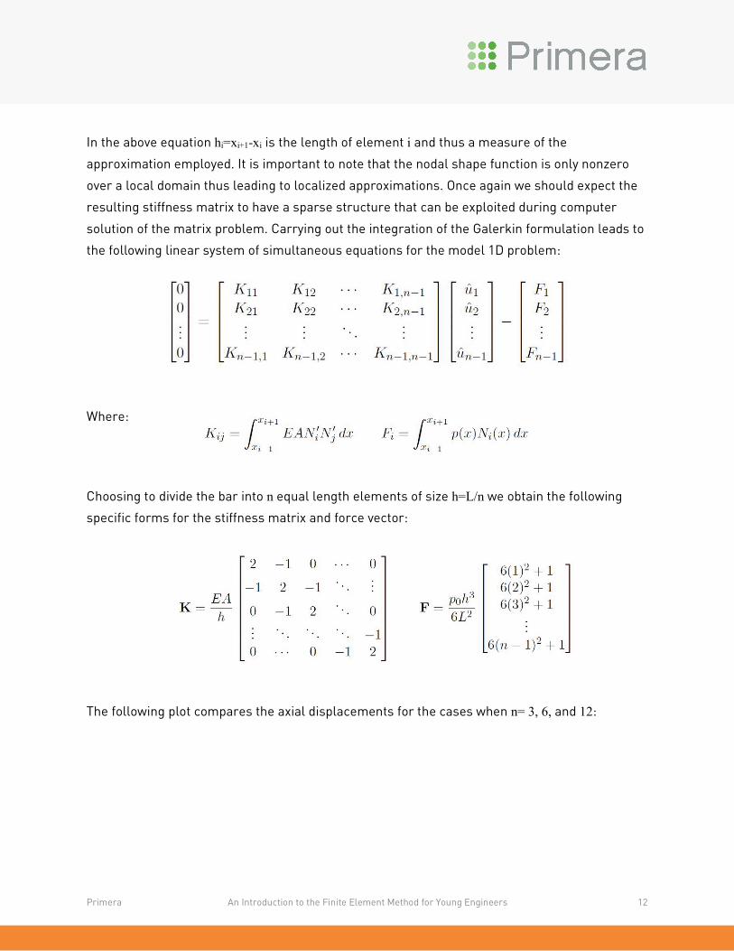
In the above equation hi=xi+1-xi is the length of element i and thus a measure of the

approximation employed. It is important to note that the nodal shape function is only nonzero

over a local domain thus leading to localized approximations. Once again we should expect the

resulting stiffness matrix to have a sparse structure that can be exploited during computer

solution of the matrix problem. Carrying out the integration of the Galerkin formulation leads to

the following linear system of simultaneous equations for the model 1D problem:

Where:

Choosing to divide the bar into n equal length elements of size h=L/n we obtain the following

specific forms for the stiffness matrix and force vector:

The following plot compares the axial displacements for the cases when n= 3, 6, and 12:


Careful observation of the plot above will highlight the fact that even for a very crude

approximation using only 3 piecewise linear functions we obtain the exact solution for the axial

displacements at the nodes. This phenomena is termed superconvergence and occurs only

when the shape functions have the same form as the Green’s function associated with the

model problem. In more complex realistic examples, superconvergence is not achieved

nevertheless the finite element method can result in accurate solutions provided a “good” mesh

is employed.

III. Discussion

This article has limited discussion to a very simply one dimensional problem to keep the

mathematical formulations relatively simple. Nevertheless, some of the same concepts

uncovered during the discussion of the model problem can be extended to solve beam

problems, 2-D and 3-D frames, plates, and shells. The finite element method has found

applications in fluid dynamics, structural dynamics, and field problems involving

electromagnetic forces.


Future articles in the series will explore more complex ideas such as:

• Beam formulations: What exactly are the geometric parameters such as shear area,

shear centers, and torsional constants?

• Error estimation and adaptive mesh refinement

• Plate elements and mesh locking

• Penalty methods: When is a stiff spring too stiff?

• FEM for structural dynamics

• Solver technology, automatic node numbering, and mesh generation

• Stress averaging: When things look better than they are

• Nonlinear formulations

IV. References

1. Hughes, T.J.R., “The Finite Element Method-Linear Static and Dynamic Finite Element

Analysis,” Prentice-Hall, Inc., copyright 1987.

2. Bathe, K-J, “Finite Element Procedures,” Prentice-Hall, Inc., copyright 1996.

3. Strang, G. and Fix, G., “An Analysis of the Finite Element Method,” Wellesley-Cambridge

Press, copyright 2008.

4. Fox, C., “An Introduction to the Calculus of Variations,” Oxford University Press, copyright

1963.


AN INTRODUCTION TO THE FINITE ELEMENT METHOD FOR … … · C. Finite Element Method The finite element method also employs the variational form of the problem similar to the Rayleigh-Ritz

Documents