An introduction to principal component analysis Ralph Burton, IAS Simon Vosper, Met Office Stephen Mobbs, IAS

An introduction to principal component analysis Ralph Burton, IAS Simon Vosper, Met Office Stephen Mobbs, IAS.
Dec 21, 2015
Welcome message from author
This document is posted to help you gain knowledge. Please leave a comment to let me know what you think about it! Share it to your friends and learn new things together.
Transcript
An introduction to principal component analysis
Ralph Burton, IAS
Simon Vosper, Met Office
Stephen Mobbs, IAS
Outline of talk
1. PCA: what the analysis can do
2. Simple examples of use
3. Application to radiosonde data: detection of inversions
4. Summary
INTRODUCTION: PCA
An objective method for determining underlying patterns in data.
Many meteorological (usually climatological) applications.
Very simple matter to determine the underlying structures…
…interpreting the structures is the difficult part;often the results have no obvious physical significance.
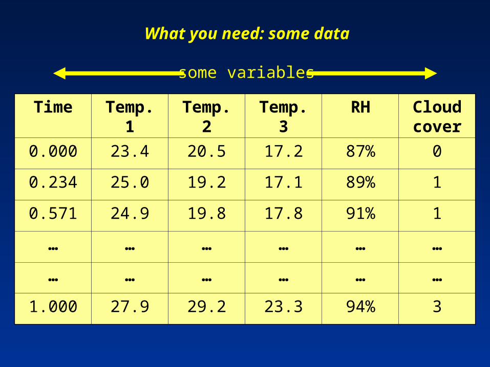
What you need: some data
Time Temp. 1 Temp. 2 Temp. 3 RH Cloud cover
0.000 23.4 20.5 17.2 87% 0
0.234 25.0 19.2 17.1 89% 1
0.571 24.9 19.8 17.8 91% 1
… … … … … …
… … … … … …
1.000 27.9 29.2 23.3 94% 3
some variables
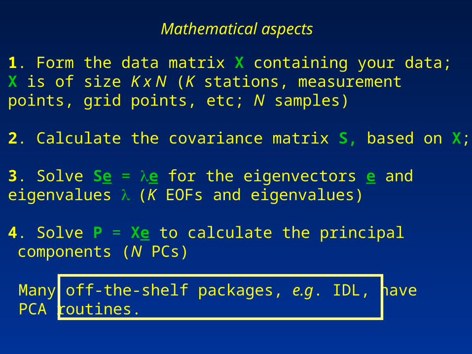
Mathematical aspects
1. Form the data matrix X containing your data;X is of size K x N (K stations, measurementpoints, grid points, etc; N samples)
2. Calculate the covariance matrix S, based on X;
3. Solve Se = e for the eigenvectors e andeigenvalues (K EOFs and eigenvalues)
4. Solve P = Xe to calculate the principal components (N PCs)
Many off-the-shelf packages, e.g. IDL, have PCA routines.
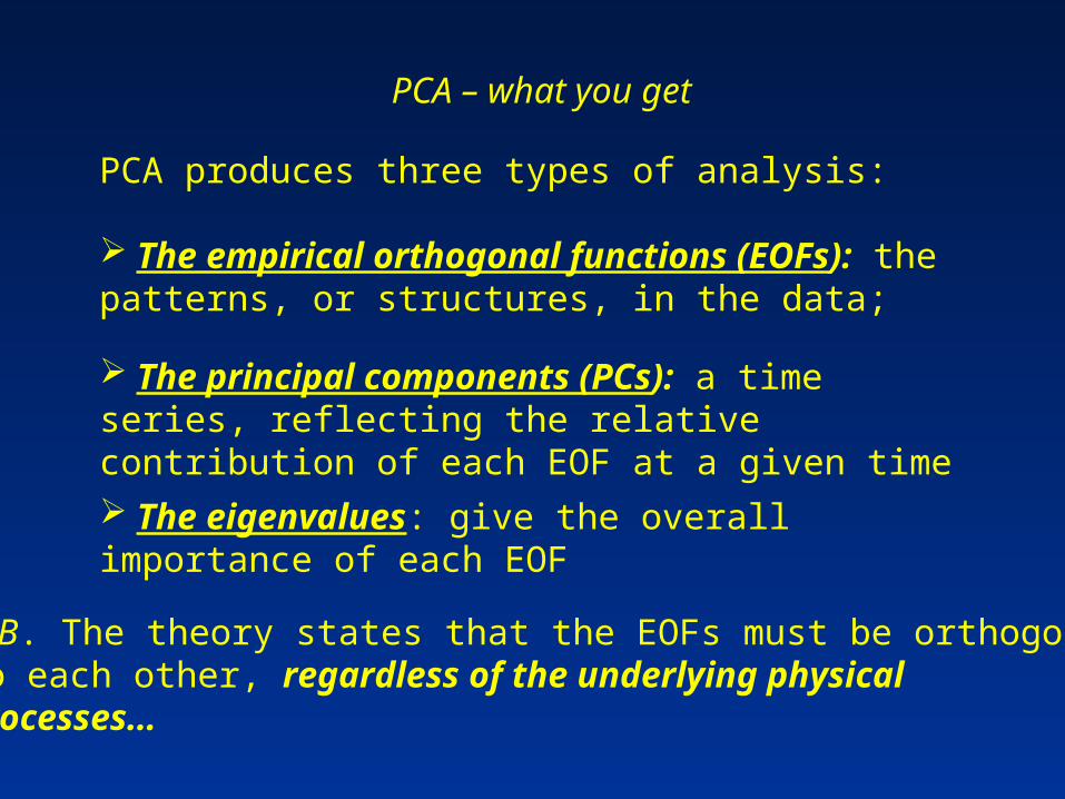
PCA – what you get
PCA produces three types of analysis:
The empirical orthogonal functions (EOFs): the patterns, or structures, in the data;
The principal components (PCs): a time series, reflecting the relative contribution of each EOF at a given time
The eigenvalues: give the overall importance of each EOF
N.B. The theory states that the EOFs must be orthogonalto each other, regardless of the underlying physicalprocesses…
EOFs: Simple example
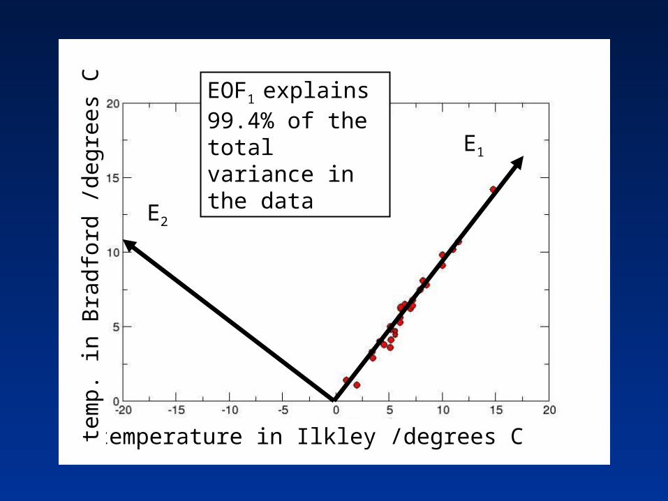
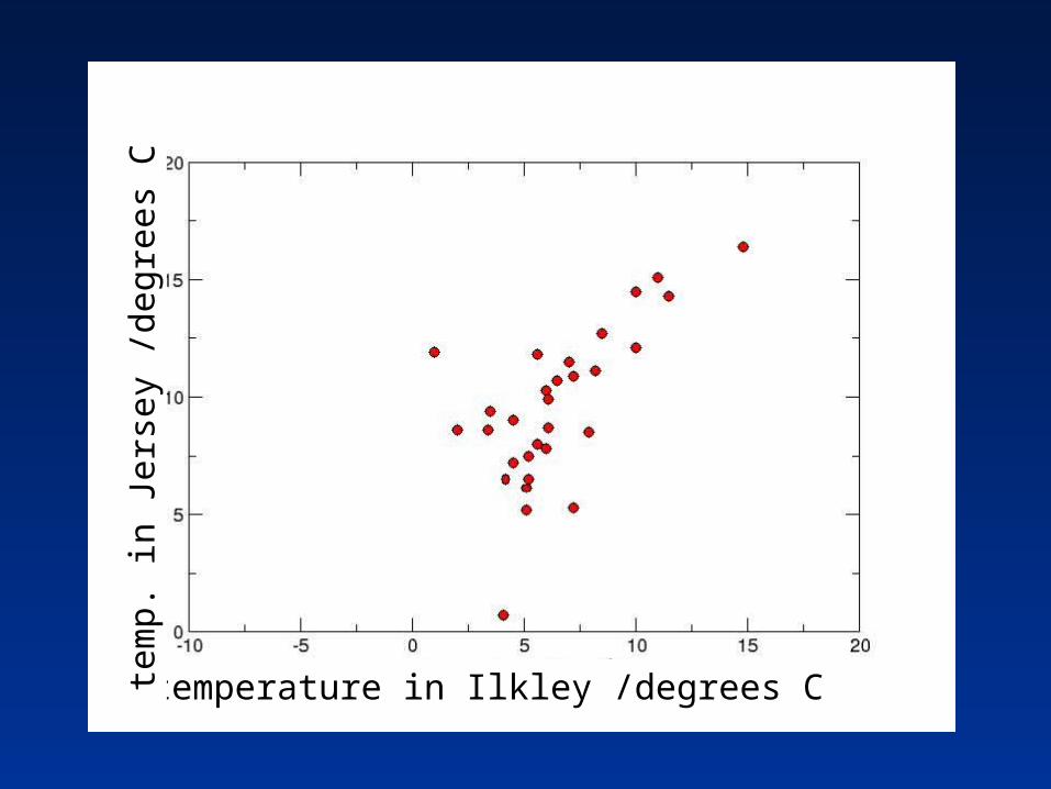
Daily maximum termperatures for November 1985from Ilkley, Bradford and Jersey were subjected totwo separate PC analyses:
I. Ilkley and Bradford
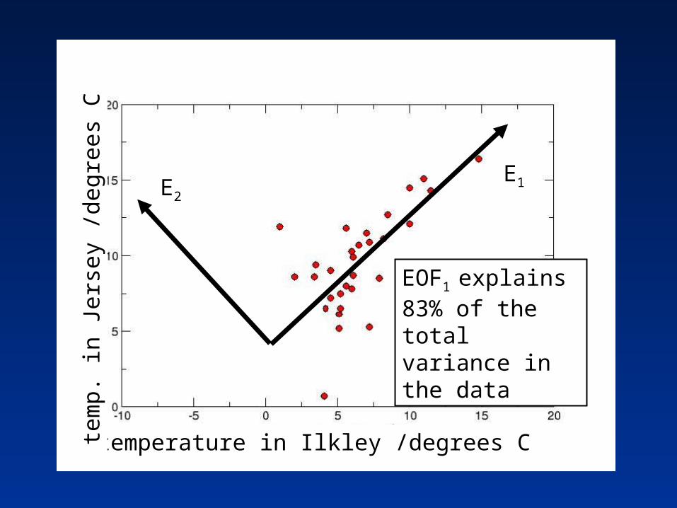
II. Ilkley and Jersey
This will reveal if there is any relationship betweenthe temperatures at these locations for the selectedtimes.
Here, the PCA will have two variables sampled at thirty points.
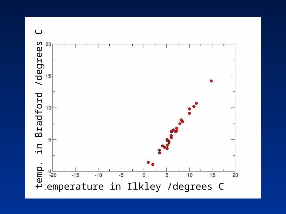
temperature in Ilkley /degrees C
tem
p. in
Bra
dfor
d /d
egre
es C
E1
E2
EOF1 explains 99.4% of the total variance in the data
temperature in Ilkley /degrees C
tem
p. in
Bra
dfor
d /d
egre
es C
temperature in Ilkley /degrees C
tem
p. in
Jer
sey
/deg
rees
C
E1E2
EOF1 explains 83% of the total variance in the data
temperature in Ilkley /degrees C
tem
p. in
Jer
sey
/deg
rees
C
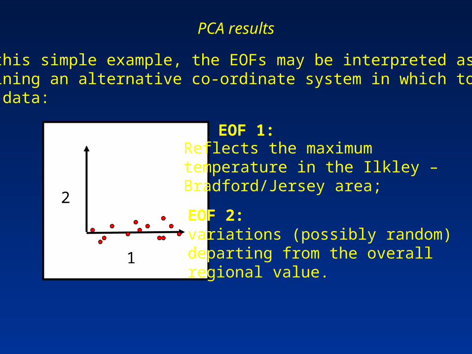
PCA results
In this simple example, the EOFs may be interpreted asdefining an alternative co-ordinate system in which to viewthe data:
1
2
EOF 1:Reflects the maximumtemperature in the Ilkley –Bradford/Jersey area;
EOF 2:variations (possibly random)departing from the overallregional value.
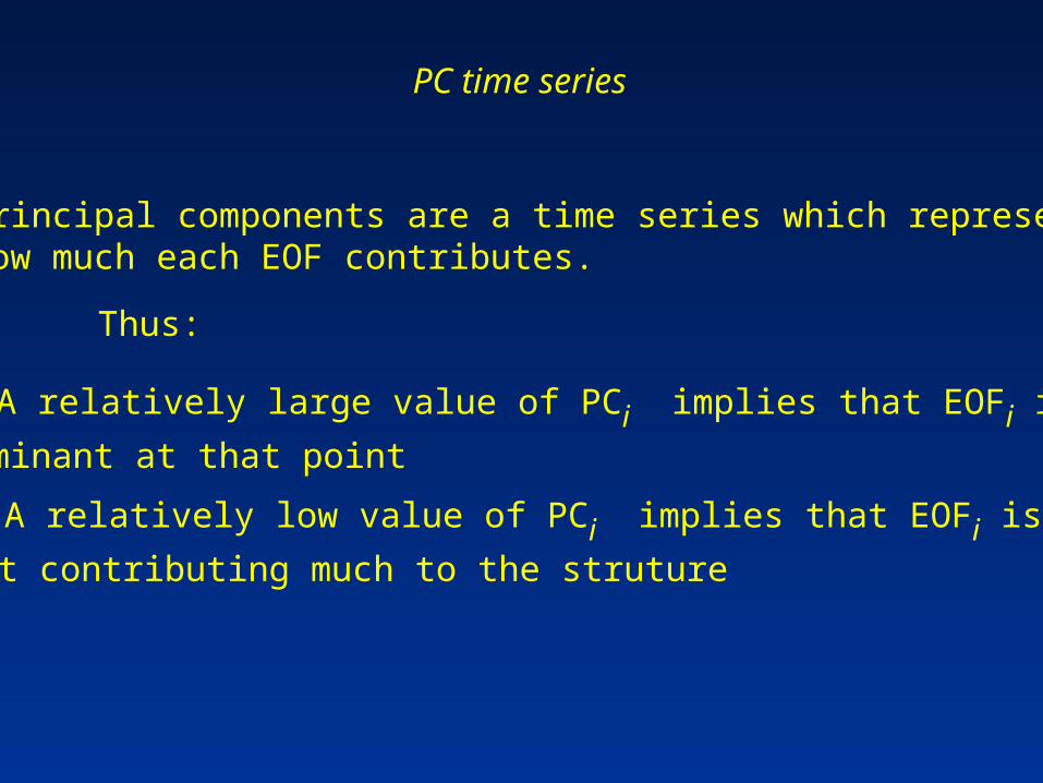
PC time series
Principal components are a time series which representhow much each EOF contributes.
Thus:
A relatively large value of PCi implies that EOFi is
dominant at that point
A relatively low value of PCi implies that EOFi is
not contributing much to the struture
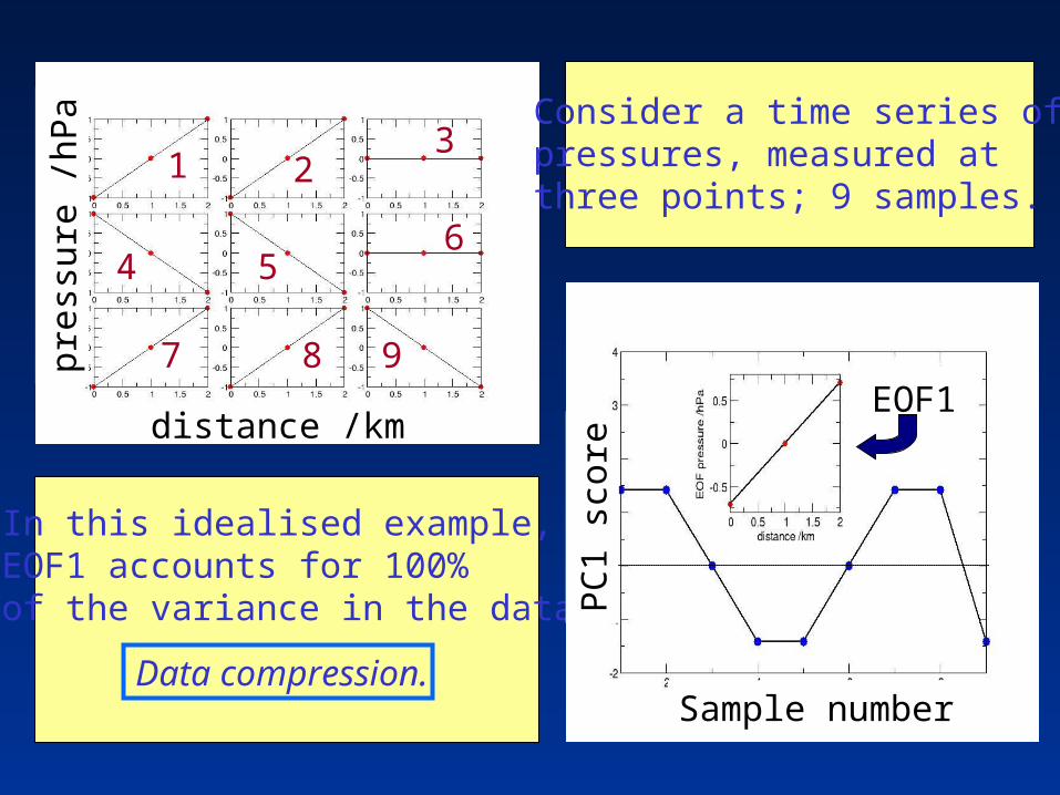
In this idealised example, EOF1 accounts for 100%of the variance in the data.
Consider a time series ofpressures, measured atthree points; 9 samples.
Data compression.
distance /km
pres
sure
/hP
a
Sample number
PC
1 sc
ore
EOF1
1
987
654
32
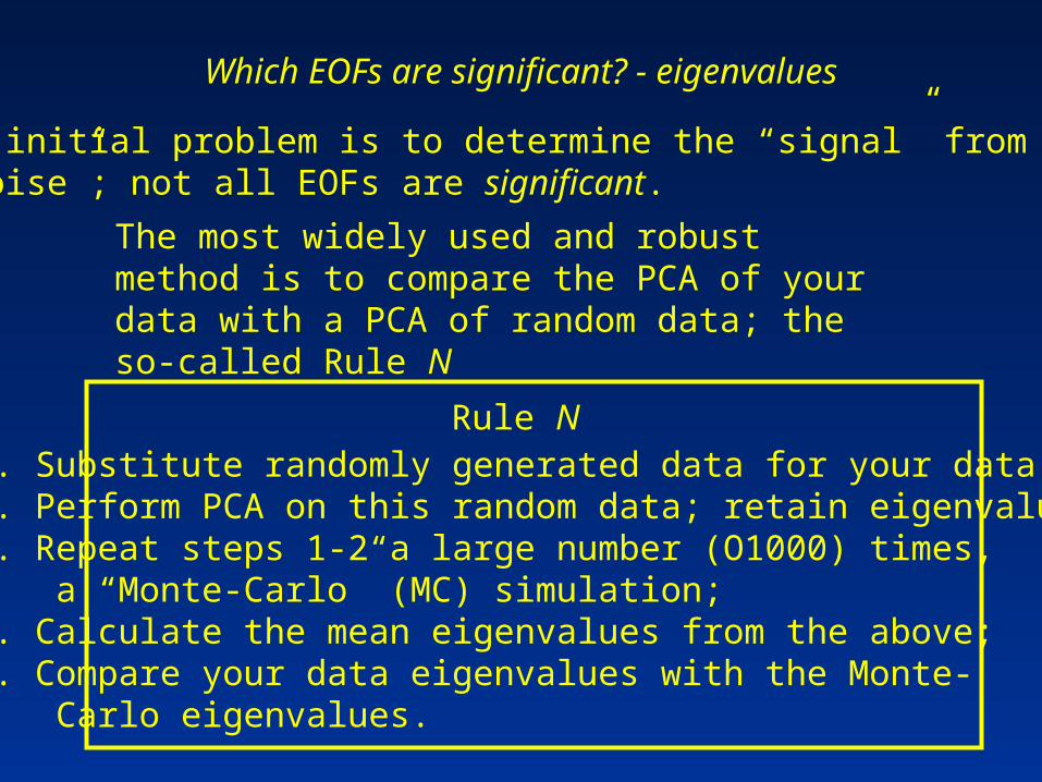
Which EOFs are significant? - eigenvalues
An initial problem is to determine the “signal” from the“noise”; not all EOFs are significant.
The most widely used and robust method is to compare the PCA of your data with a PCA of random data; the so-called Rule N
Rule N1. Substitute randomly generated data for your data;2. Perform PCA on this random data; retain eigenvalues3. Repeat steps 1-2 a large number (O1000) times, a “Monte-Carlo” (MC) simulation;4. Calculate the mean eigenvalues from the above;5. Compare your data eigenvalues with the Monte- Carlo eigenvalues.

Example: national lottery results.
Are there patterns in lottery results?…
A PCA of two years-worth of lottery results wasperformed (not including the bonus ball):
But…
EOF 1
EOF1 explains 23% of the variance in the data!!Pick: lowest value,highest value, then 4 lower values…
It could be you…
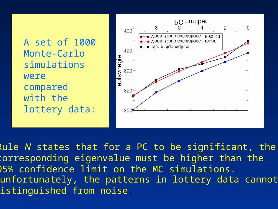
Rule N states that for a PC to be significant, thecorresponding eigenvalue must be higher than the95% confidence limit on the MC simulations.…unfortunately, the patterns in lottery data cannot bedistinguished from noise.
A set of 1000Monte-Carlo simulations were comparedwith the lottery data:
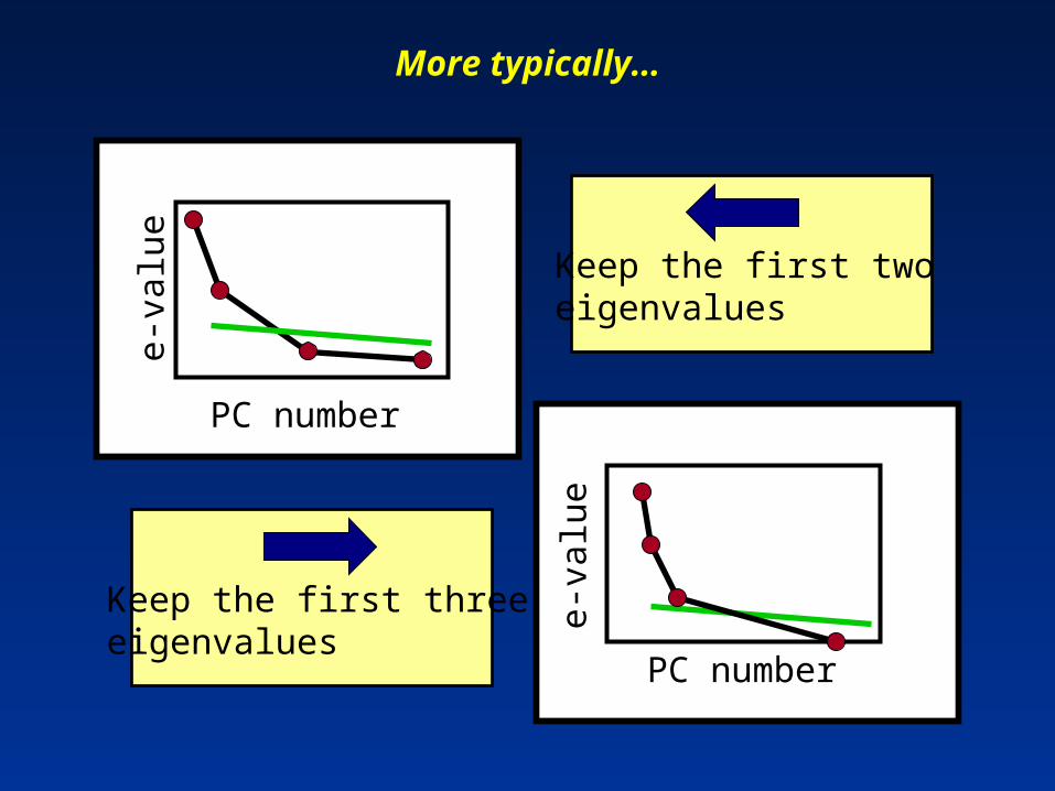
More typically…
PC number
PC number
e-va
lue
e-va
lue
Keep the first twoeigenvalues
Keep the first threeeigenvalues
Thus, we must be very careful in interpreting PCAresults:
Are the results significant (in the sense just described)?
Can the results be interpreted in a physical manner?
* * *
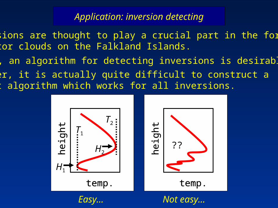
Application: inversion detecting
Inversions are thought to play a crucial part in the formationof rotor clouds on the Falkland Islands.
Thus, an algorithm for detecting inversions is desirable
However, it is actually quite difficult to construct a robust algorithm which works for all inversions.
temp.
heig
ht
temp.
heig
ht
temp.
heig
ht
temp.
heig
htH1
H2
T1
T2
??
Easy… Not easy…
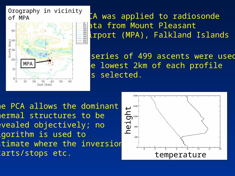
PCA was applied to radiosonde data from Mount PleasantAirport (MPA), Falkland Islands
The PCA allows the dominantthermal structures to be revealed objectively; no algorithm is used to estimate where the inversion starts/stops etc.
A series of 499 ascents were used.The lowest 2km of each profile was selected.
temperature
heig
ht
MPA
Orography in vicinity of MPA
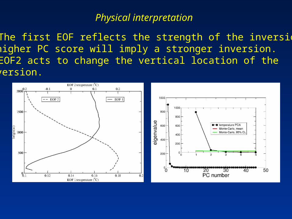
Physical interpretation
The first EOF reflects the strength of the inversion;a higher PC score will imply a stronger inversion. EOF2 acts to change the vertical location of theinversion.
Time
PC
1 sc
ore
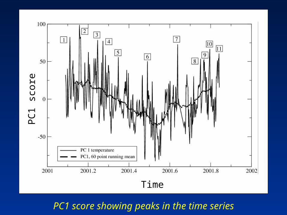
PC1 score showing peaks in the time series
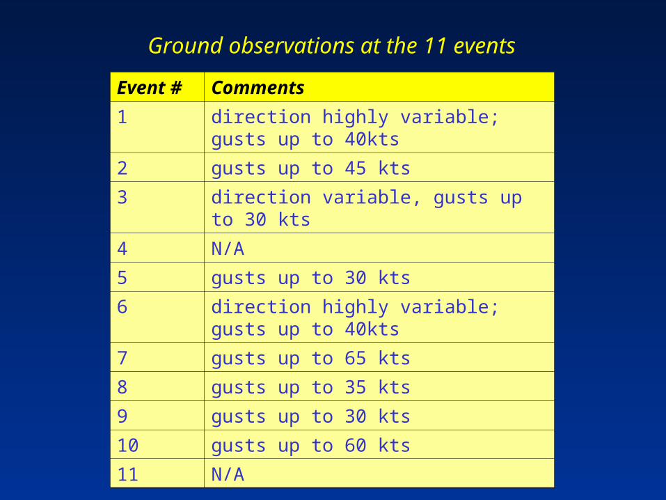
Event # Comments
1 direction highly variable; gusts up to 40kts
2 gusts up to 45 kts
3 direction variable, gusts up to 30 kts
4 N/A
5 gusts up to 30 kts
6 direction highly variable; gusts up to 40kts
7 gusts up to 65 kts
8 gusts up to 35 kts
9 gusts up to 30 kts
10 gusts up to 60 kts
11 N/A
Ground observations at the 11 events
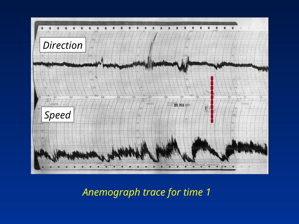
Anemograph trace for time 1
Direction
Speed
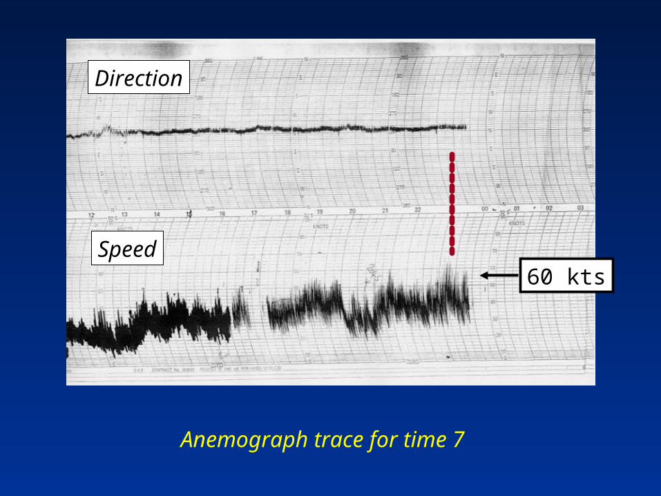
Anemograph trace for time 7
60 kts
Direction
Speed
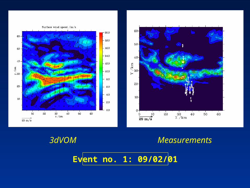
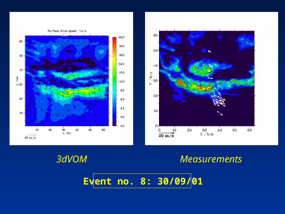
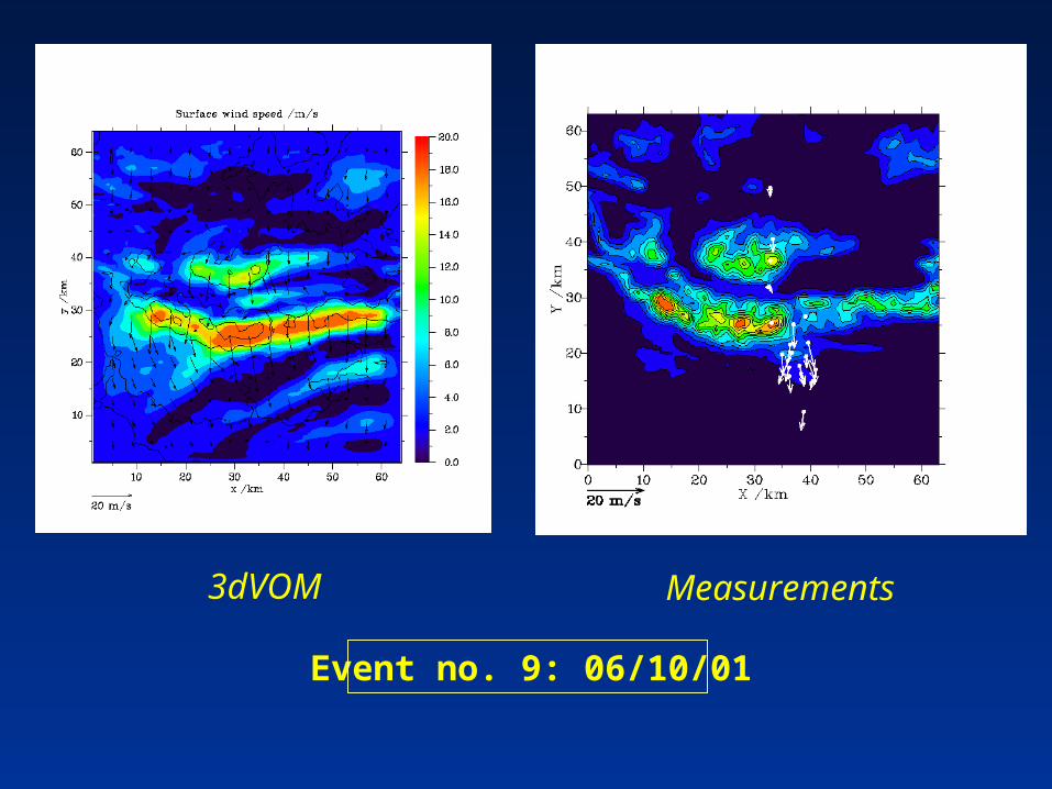
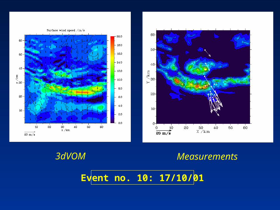
3dVOM Measurements
Event no. 1: 09/02/01
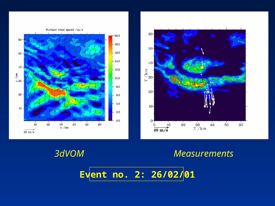
3dVOM Measurements
Event no. 2: 26/02/01
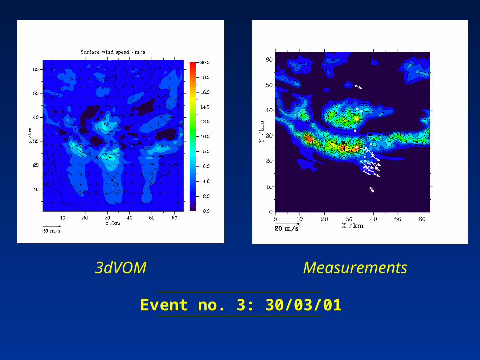
3dVOM Measurements
Event no. 3: 30/03/01
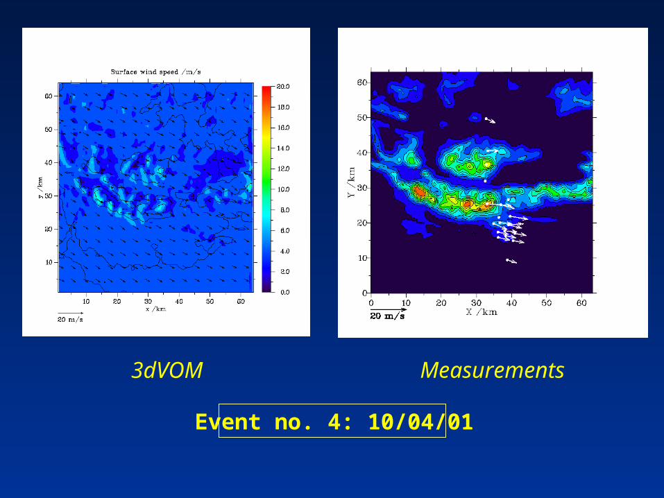
3dVOM Measurements
Event no. 4: 10/04/01
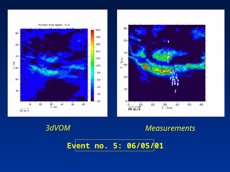
3dVOM Measurements
Event no. 5: 06/05/01
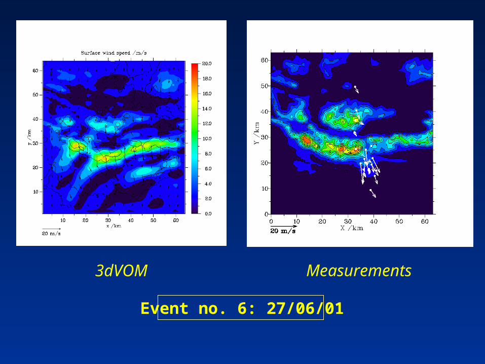
3dVOM Measurements
Event no. 6: 27/06/01
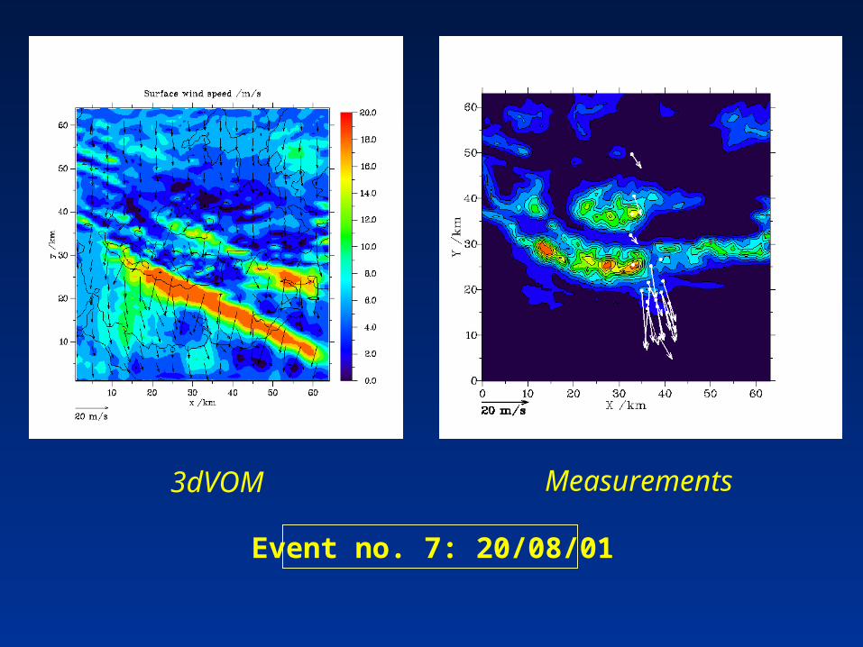
3dVOM Measurements
Event no. 7: 20/08/01
3dVOM Measurements
Event no. 8: 30/09/01
3dVOM Measurements
Event no. 9: 06/10/01
3dVOM Measurements
Event no. 10: 17/10/01
It appears that high PC1, coupled with aNortherly upstream wind direction, occursduring severe weather at the ground, asreflected in both the model and the observations.
* * *
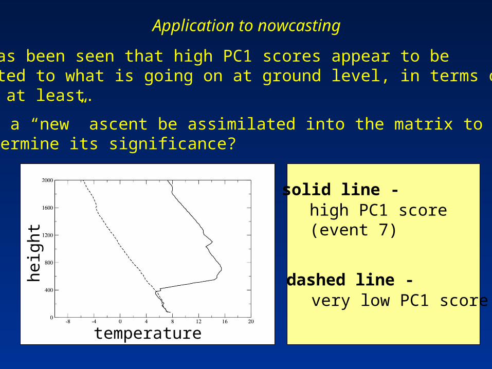
Application to nowcasting
It has been seen that high PC1 scores appear to be related to what is going on at ground level, in terms ofwind at least.
Can a “new” ascent be assimilated into the matrix todetermine its significance?
temperature
heig
ht
solid line -high PC1 score (event 7)
dashed line -very low PC1 score
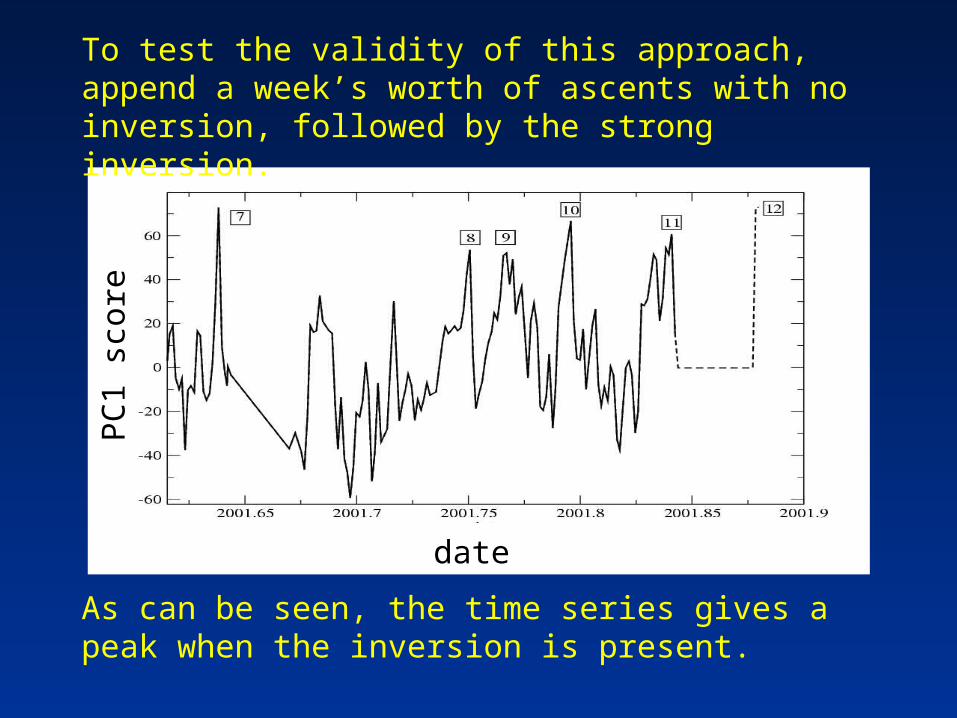
To test the validity of this approach, append a week’s worth of ascents with no inversion, followed by the strong inversion.
As can be seen, the time series gives a peak when the inversion is present.
date
PC
1 sc
ore
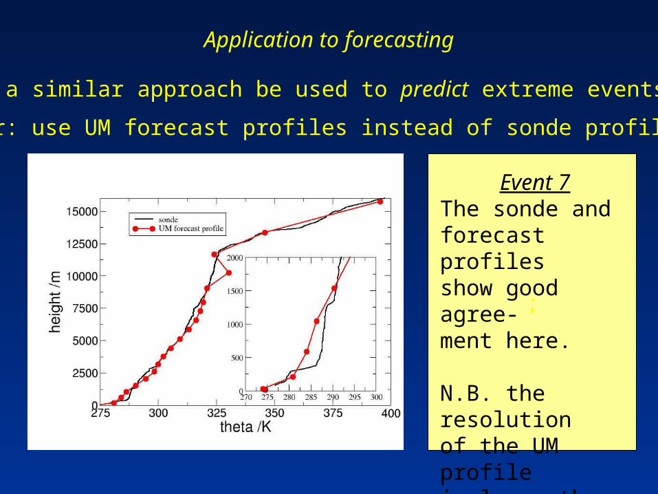
Application to forecasting
Can a similar approach be used to predict extreme events?
Answer: use UM forecast profiles instead of sonde profiles.
;
Event 7The sonde and forecast profilesshow good agree-ment here.
N.B. the resolutionof the UM profileis lower than thatfor the sonde.
Time
PC
sco
re
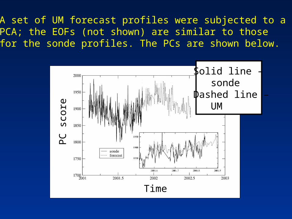
A set of UM forecast profiles were subjected to a PCA; the EOFs (not shown) are similar to thosefor the sonde profiles. The PCs are shown below.
Solid line – sondeDashed line – UM
Result of the intercomparison
The first PC for sonde and UM profiles showgood agreement;
The first PC for sonde ascents can be related tosevere weather at the ground;
The first PC for UM profiles may be used in a PCAto deduce severe weather.
Summary
PCA has been successfully applied to a series of radio-sonde ascents:
The first EOF reflects the strength of the inversion;The time series of PCs shows a series of distinct peaks
(or “events”);During most of these events, both modelling studies
and observations show severe weather at the ground…application to forecasting.
Related Documents