An Introduction to Game Theory Bruce Hajek Department of Electrical and Computer Engineering University of Illinois at Urbana-Champaign December 2017 c 2017 by Bruce Hajek All rights reserved. Permission is hereby given to freely print and circulate copies of these notes so long as the notes are left intact and not reproduced for commercial purposes. Email to [email protected], pointing out errors or hard to understand passages or providing comments, is welcome.

Welcome message from author
This document is posted to help you gain knowledge. Please leave a comment to let me know what you think about it! Share it to your friends and learn new things together.
Transcript
An Introduction to Game Theory
Bruce Hajek
Department of Electrical and Computer EngineeringUniversity of Illinois at Urbana-Champaign
December 2017
c© 2017 by Bruce Hajek
All rights reserved. Permission is hereby given to freely print and circulate copies of these notes so long as the notes are left intact
and not reproduced for commercial purposes. Email to [email protected], pointing out errors or hard to understand passages or
providing comments, is welcome.
Contents
1 Introduction to Normal Form Games 3
1.1 Static games with finite action sets . . . . . . . . . . . . . . . . . . . . . . . . . . . . . . . . . 3
1.2 Cournot model of competition . . . . . . . . . . . . . . . . . . . . . . . . . . . . . . . . . . . . 9
1.3 Correlated equilibria . . . . . . . . . . . . . . . . . . . . . . . . . . . . . . . . . . . . . . . . . 11
1.4 On the existence of a Nash equilibrium . . . . . . . . . . . . . . . . . . . . . . . . . . . . . . . 12
1.5 On the uniqueness of a Nash equilibrium . . . . . . . . . . . . . . . . . . . . . . . . . . . . . . 15
1.6 Two-player zero sum games . . . . . . . . . . . . . . . . . . . . . . . . . . . . . . . . . . . . . 17
1.6.1 Saddle points and the value of two-player zero sum game . . . . . . . . . . . . . . . . 17
1.7 Appendix: Derivatives, extreme values, and convex optimization . . . . . . . . . . . . . . . . 18
1.7.1 Derivatives of functions of several variables . . . . . . . . . . . . . . . . . . . . . . . . 18
1.7.2 Weierstrass extreme value theorem . . . . . . . . . . . . . . . . . . . . . . . . . . . . . 19
1.7.3 Optimality conditions for convex optimization . . . . . . . . . . . . . . . . . . . . . . . 20
2 Evolution as a Game 23
2.1 Evolutionarily stable strategies . . . . . . . . . . . . . . . . . . . . . . . . . . . . . . . . . . . 23
2.2 Replicator dynamics . . . . . . . . . . . . . . . . . . . . . . . . . . . . . . . . . . . . . . . . . 25
3 Dynamics for Repeated Games 31
3.1 Iterated best response . . . . . . . . . . . . . . . . . . . . . . . . . . . . . . . . . . . . . . . . 31
3.2 Potential games . . . . . . . . . . . . . . . . . . . . . . . . . . . . . . . . . . . . . . . . . . . . 32
3.3 Fictitious play . . . . . . . . . . . . . . . . . . . . . . . . . . . . . . . . . . . . . . . . . . . . 34
3.4 Regularized fictitious play and ode analysis . . . . . . . . . . . . . . . . . . . . . . . . . . . . 37
3.4.1 A bit of technical background . . . . . . . . . . . . . . . . . . . . . . . . . . . . . . . . 37
3.4.2 Regularized fictitious play for one player . . . . . . . . . . . . . . . . . . . . . . . . . . 38
3.4.3 Regularized fictitious play for two players . . . . . . . . . . . . . . . . . . . . . . . . . 39
3.5 Prediction with Expert Advice . . . . . . . . . . . . . . . . . . . . . . . . . . . . . . . . . . . 40
iii

CONTENTS v
3.5.1 Deterministic guarantees . . . . . . . . . . . . . . . . . . . . . . . . . . . . . . . . . . . 40
3.5.2 Application to games with finite action space and mixed strategies . . . . . . . . . . . 44
3.5.3 Hannan consistent strategies in repeated two-player, zero sum games . . . . . . . . . . 46
3.6 Blackwell’s approachability theorem . . . . . . . . . . . . . . . . . . . . . . . . . . . . . . . . 48
3.7 Online convex programing and a regret bound (Skip this section Fall 2017) . . . . . . . . . . 52
3.7.1 Application to game theory with finite action space . . . . . . . . . . . . . . . . . . . 55
3.8 Appendix: Large deviations and the Azuma-Hoeffding inequality . . . . . . . . . . . . . . . . 56
4 Sequential (Extensive Form) Games 59
4.1 Perfect information extensive form games . . . . . . . . . . . . . . . . . . . . . . . . . . . . . 59
4.2 Imperfect information extensive form games . . . . . . . . . . . . . . . . . . . . . . . . . . . . 63
4.2.1 Definition of extensive form games with imperfect information, and total recall . . . . 63
4.2.2 Sequential equilibria – generalizing subgame perfection to games with imperfect infor-mation . . . . . . . . . . . . . . . . . . . . . . . . . . . . . . . . . . . . . . . . . . . . . 68
4.3 Games with incomplete information . . . . . . . . . . . . . . . . . . . . . . . . . . . . . . . . 73
5 Multistage games with observed actions 77
5.1 Extending backward induction algorithm – one stage deviation condition . . . . . . . . . . . . 77
5.2 Feasibility theorems for repeated games . . . . . . . . . . . . . . . . . . . . . . . . . . . . . . 81
6 Mechanism design and theory of auctions 85
6.1 Vickrey-Clarke-Groves (VCG) Mechanisms . . . . . . . . . . . . . . . . . . . . . . . . . . . . 85
6.2 Optimal mechanism design (Myerson (1981)) . . . . . . . . . . . . . . . . . . . . . . . . . . . 89
6.3 Appendix: Envelope theorem . . . . . . . . . . . . . . . . . . . . . . . . . . . . . . . . . . . . 96
7 Introduction to Cooperative Games 99
7.1 The core of a cooperative game with transfer payments . . . . . . . . . . . . . . . . . . . . . 99
7.2 Markets with transferable utilities . . . . . . . . . . . . . . . . . . . . . . . . . . . . . . . . . 105
7.3 The Shapley value . . . . . . . . . . . . . . . . . . . . . . . . . . . . . . . . . . . . . . . . . . 109

vi CONTENTS

Preface
Game theory lives at the intersection of social science and mathematics, and makes significant appearances ineconomics, computer science, operations research, and other fields. It describes what happens when multipleplayers interact, with possibly different objectives and with different information upon which they takeactions. It offers models and language to discuss such situations, and in some cases it suggests algorithmsfor either specifying the actions a player might take, of for computing possible outcomes of a game.
Examples of games surround us in everyday life, in engineering design, in business, and politics. Gamesarise in population dynamics, in which different species of animals interact. The cells of a growing organismcompete for resources. Games are at the center of many sports, such as the game between pitcher andbatter in baseball. A large distributed resource such as the internet relies on the interaction of thousands ofautonomous players for operation and investment.
These notes also touch upon mechanism design, which entails the design of a game, usually with the goal ofsteering the likely outcome of the game in some favorable direction.
Most of the notes are concerned with the branch of game theory involving noncooperative games, in whicheach player has a separate objective, often conflicting with the objectives of other players. Some portion ofthe course will focus on cooperative game theory, which is typically concerned with the problem of how to todivide wealth, such as revenue, a surplus of goods, or resources, among a set of players in a fair way, giventhe contributions of the players in generating the wealth.
This is the first version of these notes, written in Fall 2017 in conjunction with the teaching of ECE 586GTGame Theory, at the University of Illinois at Urbana-Champaign. Problem sets and exams with solutionsare posted on the course website: https://courses.engr.illinois.edu/ece586gt/fa2017/ and https:
//courses.engr.illinois.edu/ece586/sp2013/. The author would be grateful for comments, suggestions,and corrections.
–Bruce Hajek
1

2 CONTENTS

Chapter 1
Introduction to Normal Form Games
The monograph [10] gives an introduction to game theory that influenced the presentation in this chapter.It follows with applications to a variety of routing problems in networks.
1.1 Static games with finite action sets
Perhaps the simplest games to describe involve the simultaneous actions of two player. Each player selects anaction, and then each player receives a reward determined by the pair of actions taken by the two players. Apure strategy for a player is simply one of the possible actions the player could take, whereas a mixed strategyis a probability distribution over the set of pure strategies. There is no theorem that determines the pairof strategies the two players of a given game will select, and no theorem that can determine a probabilitydistribution of joint selections, unless some assumptions are made about the objectives, rationality, andcomputational capabilities of the players. Instead, the typical outcome of a game theoretic analysis is toproduce a set of strategy pairs that are in some sort of equilibrium. The most celebrated notion of equilibriumis due to Nash; a pair of strategies is a Nash equilibrium if whenever one player uses one of the strategies,the strategy for the other player is an optimal response. There are, however, other notions of equilibrium aswell. Given these notions of equilibrium we can then investigate some immediate questions, such as: Does agiven game have an equilibrium pair? If so, is it unique? How might the players arrive at a given equilibriumpair? Are there any computational obstacles to overcome?
A two-player normal form game (or strategic form game) is specified by an action space for each player,and a payoff function for each player, such that the payoff is a function of the pair of actions taken by theplayers. If the action space of each player is finite, then the payoff functions can be specified by matrices.The two payoff matrices can be written as a single matrix with a pair of numbers for each entry, where thefirst number is the payoff for the first player, who selects a row of the matrix, and the second number is thepayoff of the second player, who selects a column of the matrix. In that way, the players select an entry ofthe matrix. A rich variety of interactions can be modeled with fairly small action spaces. We shall describesome of the most famous examples. Dozens of others are described on the internet.
Example 1.1 (Prisoners’ dilemma)
There are many similar variations of the prisoners’ dilemma game, but one instance of it is given by the
3

4 CHAPTER 1. INTRODUCTION TO NORMAL FORM GAMES
following assumptions. Suppose the players committed a crime and are being held on suspicion of committingthe crime, and are separately questioned by an investigator. Each player has two possible actions duringquestioning:
• cooperate (C) with the other player, by telling the investigator both players are innocent
• don’t cooperate (D) with the other player, by telling the investigator the two players committed thecrime
Suppose a player goes free if and only if the other player cooperates, and suppose a player is awarded pointsaccording to the following outcomes. A player receives
+1 point for not cooperating (D) with the other player by confessing
+1 point if player goes free, i.e. if the other player cooperates (C)
-1 point if player does not go free, i.e. if the other player doesn’t cooperate (D)
For example, if both players cooperate then both players receive one point. If the first player cooperates (C)and the second one doesn’t (D), then the payoffs of the players are -1, 2, respectively. The payoffs for allfour possible pairs of actions are listed in the following matrix form:
Player 1
Player 2C (cooperate) D
C (cooperate) 1,1 -1,2D 2,-1 0,0
What actions do you think rational players would pick? To be definite, let’s suppose each player cares onlyabout maximizing his/her own payoff and doesn’t care about the payoff of the other player.
Some thought shows that action D maximizes the payoff of one player no matter which action the otherplayer selects. We say that D is a dominant strategy for each player. Therefore (D,D) is a dominantstrategy equilibrium, and for that pair of actions, both players get a payoff of 0. Interestingly, if the playerscould somehow make a binding agreement to cooperate with each other, they could both be better off, receivinga payoff of 1.
Example 1.2 (Variation of Prisoners’ dilemma)
Consider the following variation of the game, where we give player 1 the option to commit suicide. What
Player 1
Player 2C (cooperate) D
C (cooperate) 1,1 -1,2D 2,-1 0,0
suicide -100,1 -100, 0
actions do you think rational players would pick? To be definite, let’s suppose each player cares only aboutmaximizing his/her own payoff and doesn’t care about the payoff of the other player.

1.1. STATIC GAMES WITH FINITE ACTION SETS 5
Some thought shows that action D maximizes the payoff of player 1 no matter which action player 2 selects.So D is still a dominant strategy for player 1. Player 2 does not have a dominant strategy. But player 2could reason that player 1 will eliminate actions C and suicide, because they are (strictly) dominated. Inother words, player 2 could reason that player 1 will select action D. Accordingly, player 2 would also selectaction D. In this example (D,D) is an equilibrium found by elimination of dominated strategies.
You can imagine games in which some dominated strategies of one player are eliminated, which could causesome strategies of the other player to become dominated and those could be eliminated, and that could causeyet more strategies of the first player to be dominated and thus eliminated, and so on. If only one strategyremains for each player, that strategy pair is called an equilibrium under iterated elimination of dominatedstrategies.
Example 1.3 (Guess 2/3 of average game) Suppose n players each select a number from [n] , 1, 2, . . . , 100.The players that select numbers closest to 2/3 the average of all n numbers split the prize money equally. Inwhat sense does this game have an equilibrium? Let’s try it out in class.
Example 1.4 (Vickrey second price auction) Suppose an object, such as a painting, is put up for auctionamong a group of n players. Suppose the value of the object to player i is vi, which is known to player i, butnot known to any of the other players. Suppose each player i offers a bid, bi, for the object. In a Vickreyauction, the object is sold to the highest bidder, and the sale price is the second highest bid. In case of a tie

6 CHAPTER 1. INTRODUCTION TO NORMAL FORM GAMES
for highest bid, the object is sold to one of the highest bidders selected in some arbitrary way (for example,uniformly at random, or to the bidder with the longest hair, etc), and the price is the same as the highestbid (because it is also the second highest bid).
If player i gets the object and pays pi for it, then the payoff of that player is vi−pi. The payoff of any playernot buying the object is zero.
In what sense does this game have an equilibrium?
Answer: Bidding truthfully is a weakly dominant strategy for each player. That means, no other strategy ofa player ever generates a larger payoff, and for any other strategy, there are possible bids by other players,such that bidding truthfully is strictly better.
We pause from examples to introduce some notation and definitions.
Definition 1.5 (Normal form, also called strategic form, game) A normal form n player game consists ofa triplet G = (I, (Si)i∈I , (ui)i]∈I) such that:
• I is a set of n elements, indexing the players. Typically I = 1, . . . , n = [n].
• Si is the action space of player i, assumed to be a nonempty set
• S = S1 × · · · × Sn is the set of strategy profiles. A strategy profile can be written as s = (s1, . . . , sn).
• ui : S → R, such that ui(s) is the payoff of player i.
Some important notation ubiquitous to game theory is described next. Given a normal form n-player game(I, (Si), (ui)), an element s ∈ S can be written as s = (s1, . . . , sn). If we wish to place emphasis on the ith
coordinate of s for some i ∈ I, we write s as (si, s−i). Here s−i is s with the ith entry omitted. We use s and(si, s−i) interchangeably. Such notation is very often used in connection with payoff functions. The payoffof player i for given actions of all players s can be written as ui(s). An equivalent expression is ui(si, s−i).So, for example, if player i switches action to s′i and all the other players use the original actions, then schanges to (s′i, s−i).
In some situations it is advantageous for a player to randomize his/her action. If the action space for aplayer is Si we write Σi for the space of probability distributions over Si. A mixed strategy for player i is aprobability distribution σi over Si. In other words, σi ∈ Σi. If f : Si 7→ R, the value of f for an action si ∈ Siis simply f(si). If σi is a mixed strategy for player i, we often use the notational convention f(σi) = Eσi [f ].In particular, if Si is a finite set, then σi is a probability vector, and f(σi) =
∑si∈Si f(si)σi(si). In a normal
form game, if the players are using mixed strategies, we assume that the random choice of pure strategy foreach player i is made independently of the choices of other players, using distribution σi. Thus, for a mixedstrategy profile σ = (σ1, . . . , σn), the expected payoff for player i, written ui(σ), or, equivalently, ui(σi, σ−i)denotes expectation of ui with respect to the product probability distribution σ1 ⊗ · · · ⊗ σn.
Definition 1.6 A strategy profile (s1, . . . , sn) for an n-player normal form game (I, (Si), (ui)) is a Nashequilibrium in pure strategies if for each i and any alternative action s′i,
ui(si, s−i) ≥ ui(s′i, s−i).
A strategy profile of mixed strategies (σ1, . . . , σn) for an n-player normal form game (I, (Si), (ui)) is a Nashequilibrium in mixed strategies if for each i and any alternative mixed strategy σ′i,
ui(σi, σ−i) ≥ ui(σ′i, σ−i).

1.1. STATIC GAMES WITH FINITE ACTION SETS 7
We adopt the convention that a pure strategy si is also a mixed strategy, because it is equivalent to theprobability distribution that places probability mass one at the single point si. Pure strategies are consideredto be degenerate mixed strategies. Nondegenerate mixed strategies are those that don’t have all their prob-ability mass on one point. Completely mixed strategies are mixed strategies that assign positive probabilityto each action.
The concept of Nash equilibrium is perhaps the most famous equilibrium concept for game theory, but thereare other equilibrium concepts. To mention one other, shown above for the prisoners’ dilemma game, is adominant strategy equilibrium.
Definition 1.7 Consider a normal form game (I, (Si)i∈I , (ui)i∈I). Fix a player i and let si, s′i ∈ Si.
(i) Strategy si dominates strategy s′i (or s′i is dominated by si) for player i if:
u(s′i, s−i) < u(si, s−i) for all choices of s−i.
Strategy si is a dominant strategy for player i if it dominates all other strategies of player i.
(ii) Strategy si weakly dominates strategy s′i (or s′i is weakly dominated by si) for player i if:
ui(s′i, s−i) ≤ ui(si, s−i) for all choices of s−i and
ui(s′i, s−i) < ui(si, s−i) for some choice of s−i. (1.1)
Strategy si is a weakly dominant strategy for player i if it weakly dominates all other strategies ofplayer i.
Definition 1.8 Consider a strategy profile s = (s1, . . . , sn) for an n-player normal form game (I, (Si), (ui)).(i) The profile s is a dominant strategy equilibrium (in pure strategies) if, for each i, si is a dominant strategyfor player i.(ii) The profile s is a weakly dominant strategy equilibrium (in pure strategies) if, for each i, si is a weaklydominant strategy for player i.
Remark 1.9 A weaker definition of weak domination would be obtained by dropping the requirement (1.1),and in many instances either definition would work. To be definite, we will stick to the definition that includes(1.1), and leave it to the interested reader to determine when the weaker definition of weak domination wouldalso work.
Proposition 1.10 (Iterated elimination of weakly dominated strategies (IEWDS) and Nash equilibrium)Consider a finite game (I, (Si)i∈I , (ui)i∈I) in normal form. Suppose a sequence of games is constructed byiterated elimination of weakly dominated strategies (IEWDS). In other words, given a game in the sequence,some player i is chosen with some weakly dominated strategy si and Si is replaced by Si\si to obtain thenext game in the sequence, if any. If the final game in the sequence has only one strategy profile, then thatstrategy profile is a Nash equilibrium for the original game.
Proof. If a game has only one strategy profile, i.e. if each player has only one possible action, then thatstrategy profile is trivially a Nash equilibrium. It thus suffices to show that if G′ is obtained from G by onestep of IEWDS and if a strategy profile s is a Nash equilibrium for G′, then s is also a Nash equilibriumfor G. So, IEWDS cannot create a new Nash equilibrium. So fix such games G and G′ and let s′i be theaction available to some player i in G that was eliminated to get game G′ because some action si availablein G weakly dominated s′i. Suppose s is a Nash equilibrium for G′. Since any action for any player in G′
is available to the same player in G, σ is also a strategy profile for G, and we need to show it is a Nashequilibrium for G. For j 6= i, whether sj is a best response to s−j for player j is the same for G or G′ – the

8 CHAPTER 1. INTRODUCTION TO NORMAL FORM GAMES
set of possible responses for player j is the same. Thus, sj must be a best response to s−j for game G, ifj 6= i. Also, si must be at least as good a response as si, which in turn is at least as good as s′i, both forplayer i. Therefore, si is a best response to s−i in game G. Therefore, s is a Nash equilibrium for the gameG, as we needed to prove.
Proposition 1.10 is applicable to the guess 2/3 of the average game–see the homework problem about it.
Example 1.11 (Bach or Stravinksy) or opera vs. football, or battle of the sexes
This two player normal form game is expressed by the following matrix of payoffs: Player 1 prefers to go to
Player 1
Player 2B S
B 3,2 0,0S 0,0 2,3
a Bach concert while player 2 prefers to go to a Stravinsky concert, and both players would much prefer togo to the same concert together. There is no dominant strategy. There are two Nash equilibria: (B,B) and(S,S).
The actions B or S are called pure strategies. A mixed strategy is a probability distribution over the purestrategies. If mixed strategies are considered, we can consider a new game in which each player selects amixed strategy, and then each player seeks to maximize his/her expected payoff, assuming the actions of theplayers are selected independently.
For this example, suppose player 1 selects B with probability a and S with probability 1− a, In other words,player 1 selects probability distribution (a, 1 − a). If a = 0 or a = 1 then the distribution is equivalent to apure strategy, and is considered to be a degenerate mixed strategy. If 0 < a < 1 the strategy is a nondegeneratemixed strategy. Suppose player 2 selects probability distribution (b, 1− b). Is there a Nash equilibrium for theexpected payoff game such that at least one of the players uses a nondegenerate mixed strategy?
Suppose ((a, 1 − a), (b, 1 − b)) is a Nash equilibrium with 0 < a < 1 and 0 ≤ b ≤ 1. The expected reward ofplayer 1 is 3ab+ 2(1− a)(1− b) which is equal to 2(1− b) + a(5b− 2). In order for a to be a best responsefor player 1, it is necessary that 5b − 2 = 0 or b = 2
5 . If b = 25 then player 1 gets the same payoff for
action B or S. This fact is an example of the equalizer principle, which is that a mixed strategy is a bestresponse only if the pure strategies it is randomized over have equal payoffs. By symmetry, in order for( 2
5 ,35 ) to be a best response for player 2 (which is a nondegenerate mixed strategy), it must be that a = 3
5 .Therefore, (( 3
5 ,25 ), ( 2
5 ,35 )) is the unique Nash equilibribum in mixed strategies such that at least one strategy
is nondegenerate. The expected payoffs for both players for this equilibrium is 3 · 625 + 2 · 6
25 = 65 , which is
not very satisfactory for either player compared to the other two Nash equilibria in pure strategies.
A satisfactory behavior of the players faced with this game might be for them to agree to both play B or bothplay S, where the decision is made by the flip of a fair coin that both players can observe. Given the coinflip, neither player would have incentive to unilaterally deviate from the agreement. The expected payoff ofeach player would be 2.5. This strategy is an example of the players using common randomness (both playersobserve the outcome of the coin flip) to randomize among two or more Nash equilibrium points.
Example 1.12 (Matching pennies) This is a well known zero sum game. Players 1 and 2 each put apenny under their hand, with either (H) “heads” or (T) “tails” on the top side of the penny, and then they

1.2. COURNOT MODEL OF COMPETITION 9
simultaneously remove their hands to reveal the pennies. This is a zero sum game, with player 1 winning ifthe actions are the same, i.e. HH or TT, and player 2 winning if they are different. The game matrix isshown. Are there any dominant strategies? Nash equilibria in pure strategies? Nash equilibrium in mixed
Player 1
Player 2H T
H 1,-1 -1,1T -1,1 1, -1
strategies?
Example 1.13 (Rock Scissors Paper) This is a well known zero sum game, similar to matching pennies.Two players simultaneously indicate (R) “rock,” (S) “scissors,” or (P)“paper.” Rock beats scissors, becausea rock can bash a pair of scissors. Scissors beats paper, because scissors can cut paper. Paper beats rock,because a paper can wrap a rock. The game matrix is shown. Are there any dominant strategies? Nash
Player 1
Player 2R S P
R 0,0 1,-1 -1,1S -1,1 0,0 1,-1P 1,-1 -1,1 0,0
equilibria in pure strategies? Nash equilibrium in mixed strategies?
Example 1.14 (Identical interest games) A normal form game (I, (Si)i∈I , (ui)i∈I) is an identical interestgame (or a coordination game) if ui is the same function for all i. In other words, if there is a single functionu : S → R such that ui ≡ u for all i ∈ I. In such games, the players would all like to maximize the samefunction u(s). That could require coordination among the players because each player i controls only entry siof the strategy profile vector. A strategy profile s is a Nash equilibrium if it is a local maximum of u in thesense that for any i ∈ I and any s′i ∈ Si, u(s′i, s−i) ≤ u(si, s−i).
1.2 Cournot model of competition
Often in applications, Nash equilibria can be explicitly identified, so there is no need to invoke an existencetheorem. And properties of Nash equilibria can be established that sometimes determine the number of Nashequilibria, including possibly uniqueness. These points are illustrated in the example of the Cournot modelof competition. The competition is among firms producing a good; the action of each firm i is to select aquantity si to produce. The total supply produced by all firms is stot = s1 + · · ·+ sn. Suppose that the priceper unit of good produced depends on the total supply as p(stot) = a− stot, where a > 0, as pictured in Fig.1.1(a).
Suppose also that the cost per unit production is a constant c, no matter how much a firm produces. Wesuppose the set of valid values of si for each i are Si = [0,∞). To avoid trivialities we assume that a > c;otherwise the cost of production of any positive amount would exceed the price.

10 CHAPTER 1. INTRODUCTION TO NORMAL FORM GAMES
2
1
a
00
price per unit
supply
a
a−c
a−c
a−c2
B (s )1
2 s1
(a) (b)
a−c2
00
monopolist supply
B (s )
2
1
s
Figure 1.1: (a) Price vs. total supply for Cournot game, (b) Best response functions for two-player Cournotgame.
The payoff function of player i is given by ui(s) = (a − stot − c)si. As a function of si for s−i fixed, ui is
quadratic and the best response si to actions of the other players can be found by setting ∂ui(s)∂si
= 0, orequivalently,
(a− stot − c)− si = 0 or si = a− stot − c.
Thus, si is the same for all i for any Nash equilibrium, so we have si = a − nsi − c or si = a−cn+1 . The total
supply at the Nash equilibrium is
sNashtot =n(a− c)n+ 1
,
which increases from a−c2 for the case of monopoly (one firm) towards the limit a− c as n→∞. The payoff
of each player i at the Nash equilibrium is thus given by
uNashi =
(a− n(a− c)
n+ 1− c)(
a− cn+ 1
)=
(a− c)2
(n+ 1)2.
The total sum of payoffs is nuNashi = n(a−c)2(n+1)2 . For example, in the case of a monopoly (n = 1) the payoff
to the firm is (a−c)24 and the supply produced is a−c
2 . In the case of duopoly (n=2) the sum of revenues is2(a−c)2
9 and the total supply produced is 2(a−c)3 . In the case of duopoly, if the firms could enter a binding
agreement with each other to only produce a−c4 each, so the total production matched the production in the
case of monopoly, the firms could increase there payoffs.
To find the best response functions for this game, we solve the equation si = a − stot − c for si to get
Bi(s−i) =(a−c−|s−i|
2
)+, where |s−i| represents the sum of the supplies produced by the players except
player i. Fig. 1.1(b) shows the best response functions B1 and B2 for the case of duopoly (n=2). The dashed
zig-zag curve starting at s1 = 3(a−c)4 shown in the figure indicates how iterated best response converges to
the Nash equilibrium point for two players.
Note: We return to Cournot competition later. With minor restrictions it has an ordinal potential, showingthat iterated one-at-a-time best response converges to the Nash equilibrium for the n-player game.

1.3. CORRELATED EQUILIBRIA 11
1.3 Correlated equilibria
The concept of correlated equilibrium is due to Aumann [1]. We introduce it in the context of the Dove Hawkgame pictured in Figure 1.2. The action D represents cooperative, passive behavior, whereas H represents
Player 1
Player 2D H
D 4,4 1,5H 5,1 0,0
Figure 1.2: Payoff matrix for the dove-hawk game
aggressive behavior against the play D. There are no dominant strategies. Both (D,H) and (H,D) are purestrategy Nash equilibria. And ((0.5, 0.5), (0.5, 0.5)) is a Nash equilibrium in mixed strategies with payoff 2.5to each player. How might the players do better?
One idea is to have the players agree with each other to both play D. Then each would receive payoff 4.However, that would require the players to have some sort of trust relationship. For example, they mightenter into a binding contract on the side.
The following notion of correlated equilibrium relies somewhat less on trust. Suppose there is a trustedcoordinator that sends a random signal to each player, telling the player what action to take. The play-ers know the joint distribution of what signals are sent, but each player is not told what signal is sent tothe other player. For this game, a correlated equilibrium is given by the following joint distribution of signals:
Player 1
Player 2D H
D 1/3 1/3H 1/3 0
In other words, with probability 1/3, the coordinator tells player 1 to play H and player 2 to play D. Withprobability 1/3, the coordinator tells player 1 to play D and player 2 to play D. And so on. Both playersassume that the coordinator acts as declared. If player 1 is told to play H, then player 1 can deduce thatplayer 2 was told to play D, so it is optimal for player 1 to follow the signal and play H. If player 1 is toldto play D, then by Bayes rule, player 1 can reason that the conditional distribution of the signal to player2 was (0.5, 0.5), so, conditioned on the signal for player 1 being D, the signal to player 2 is equally likely tobe D or H. Hence, the conditional expected reward for player 1, given the signal D received, is 2.5 whetherplayer 1 obeys and plays D, or player 1 deviates and plays H. Thus, player 1 has no incentive to deviatefrom obeying the coordinator. The game and equilibrium are symmetric in the two players, and each hasexpected payoff (4+1+5)/3 = 10/3. This is an example of correlated equilibrium.
A slightly different type of equilibrium, which also involves a coordinator, is to randomize over Nash equi-libria, with the coordinator selecting and announcing which Nash equilibria will be implements. We alreadymentioned this idea for the Bach or Stravinksy game. For the Dove Hawk game, the coordinator couldflip a fair coin and with probability one half declare that the two players should use the Nash equilibrium(H,D) and otherwise declare that the two players should use the Nash equilibrium (D,H). In this case theannouncement of the coordinator can be public – both players know what the signal to both players is. Evenso, since (H,D) and (D,H) are both Nash equilibria, neither player has incentive to unilaterally deviatefrom the instructions of the coordinator. In this case, the expected payoff for each player is (5+1)/2 = 3.
Definition 1.15 A correlated equilibrium for a normal form game (I, (Si), (ui)) with finite action spaces is

12 CHAPTER 1. INTRODUCTION TO NORMAL FORM GAMES
a probability distribution p on S = S1 × · · · × Sn such that for any si, s′i ∈ Si:∑
s−i∈S−i
p(si, s−i)ui(si, s−i) ≥∑
s−i∈S−i
p(si, s−i)ui(s′i, s−i) (1.2)
Why does Definition 1.2 make sense? The interpretation of a correlated equilibrium is that a coordinatorrandomly generates a set of signals s = (s1, . . . , sn) using the distribution p, and privately tells each playerwhat to play. Dividing each side of (1.2) by p(si) (the marginal probability that player i is told to play si)yields ∑
s−i∈S−i
p(s−i|si)ui(si, s−i) ≥∑
s−i∈S−i
p(s−i|si)ui(s′i, s−i). (1.3)
Given player i is told to play si, the lefthand side of (1.3) is the conditional expected payoff of player iif player i obeys the coordinator. Similarly, given player i is told to play si, the righthand side of (1.3)is the conditional expected payoff of player i if player i deviates and plays s′i instead. Hence, under acorrelated equilibrium, no player has an incentive to deviate from the signal the player is privately given bythe coordinator.
Remark 1.16 A somewhat more general notion of correlated equilibria is that each player is given someprivate information by a coordinator. The information might be less specific than a particular action thatthe player should take, but the player needs to deduce an action to take based on the information receivedand on knowledge of the joint distribution of signals to all players, assuming all players rationally respondto their private signals. The actions of the coordinator are modeled by a probability space (Ω,F , p) and aset of subsigma algebras Hi of F , where Hi represents the information released to player i. Without loss ofgenerality, we can take F to be the smallest σ-algebra containing Hi for all i: F = ∨i∈IHi, so a correlatedequilibrium can be represented by (Ω, Hii∈I , p, Sii∈I) where each Si is an Hi measurable random variableon (Ω,F , p), such that the following incentive condition holds for each i ∈ I:
E [ui(Si, S−i)] ≥ E [ui(S′i, S−i)] (1.4)
for any Hi measurable random variable S′i. (Since we’ve just used Si for the action taken by a player i we’dneed to introduce some alternative notation for the set of possible actions of player i, such as Ai.) In theend, for this more general setup, all that really matters for the expected payoffs is the joint distribution ofthe random actions, so that any equilibrium in this more general setting maps to an equivalent equilibriumin the sense of Definition 1.2.
Note that a Nash equilibrium is a special case of correlated equilibrium in which the signals are deterministic.Thus, the notion of correlated equilibrium offers more equilibrium possibilities, although implementationrelies on the availability of a trusted coordinator and private information channels from the coordinator tothe players.
1.4 On the existence of a Nash equilibrium
Theorem 1.17 (Bauer fixed point theorem) Let S be a simplex or unit ball in Rn and let f : S 7→ S be acontinuous function. There exists s∗ ∈ S such that f(x∗) = s∗.
For a proof see, for example, [3]

1.4. ON THE EXISTENCE OF A NASH EQUILIBRIUM 13
Theorem 1.18 (Kakutani fixed point theorem) Let f : A ⇒ A be a set valued function satisfying thefollowing conditions:
(i) A is a compact, convex, nonempty subset of Rn for some n ≥ 1.
(ii) f(x) 6= ∅ for x ∈ A.
(iii) f(x) is a convex set for x ∈ A.
(iv) The graph of f , (x, y) : x ∈ A, y ∈ f(x) is closed.
There exists x∗ so that x∗ ∈ F (x∗).
Some examples are shown in Figure 1.3 with A = [0, 1].
b0 1
1
0 1
1
0 1
1
0 1
1
(a) Not continuous (b) f(b) not convex (c) OK (d) OK
Figure 1.3: Examples of correspondences from [0, 1] to [0, 1] illustrating conditions of Kakutani theorem.
Theorem 1.19 (Existence of Nash equilibria – Nash) Let (I, (Si : i ∈ I), (ui : i ∈ I)) be a finite game innormal form (so I and the sets Si all have finite cardinality). Then there exits a Nash equilibrium in mixedstrategies.
Proof. Let Σi denote the set of mixed strategies for player i (i.e. the set of probability distributionson Si). Let Bi(σ−i) , arg maxσi ui(σi, σ−i). Let Σ = Σ1 × · · · × Σn). Let σ denote an element of Σ, soσ = (σ1, . . . , σn). Let B(σ) = (B1(σ−1)× . . .×Bn(σ−n)). The Nash equilibrium points are the fixed pointsof B. In other words, σ is a Nash equilibrium if and only if σ ∈ B(σ). The proof is completed by invokingthe Kakutani fixed point theorem for Σ and B. It remains to check that Σ and B satisfy conditions (i)-(iv)of Theorem 1.18. (i) For each i, the set of probability distributions Σi is compact and convex, and so thesame is true of the product set Σ. (ii)-(iii) For any σ ∈ Σ and i ∈ I, the best response set Bi(σ−i) is the setof all probability distributions on Σi that are supported on the best response actions in Si, so Bi(σ−i) is anonempty convex set for each i, and hence the product set B(σ) is also nonempty and convex.
(iv) It remains to verify that the graph of B is closed. So let (σ(n), σ(n))n≥1 denote a sequence of points in thegraph (so σ(n) ∈ Σ and σ(n) ∈ B(σ(n)) for each n) that converges to a point (σ(∞), σ(∞)). It must be proved
that the limit point is in the graph, meaning that σ(∞) ∈ B(σ(∞)), or equivalently, that σ(∞)i ∈ Bi(σ(∞)
−i )for each i ∈ I. So fix an arbitrary i ∈ I.Fix an arbitrary strategy σ′i ∈ Σi. Then
ui(σ(n)i , σ
(n)−i ) ≥ ui(σ′i, σ
(n)−i ) (1.5)
for all n ≥ 1. The function ui(σi, σ−i) is an average of payoffs for actions selected independently withdistributions σi, so it is a continuous function of σ. Therefore, the left and right hand sides of (1.5) converge
to ui(σ(∞)i , σ
(∞)−i ) and ui(σ
′i, σ
(∞)−i ), respectively. Since weak inequality “≥” is a closed relation, (1.5) remains

14 CHAPTER 1. INTRODUCTION TO NORMAL FORM GAMES
true if the limit is taken on each side of the inequality, so ui(σ(∞)i , σ
(∞)−i ) ≥ ui(σ
′i, σ
(∞)−i ). Thus, σ
(∞)i ∈
Bi(σ(∞)−i ) for each i ∈ I, so σ(∞) ∈ B(σ(∞)).
Remark 1.20 Although Nash’s theorem guarantees that any finite game has a Nash equilibrium in mixedstrategies, the proof is based on a nonconstructive fixed point theorem. It is believed to be a computationallydifficult problem to find a Nash equilibrium except for certain classes of games, most importantly, zero sumtwo player games. To appreciate the difficulty, we can see that the problem of finding a mixed strategy Nashequilibrium has a combinatorial aspect. A difficult part is to find subsets Soi ⊂ Si of the action sets Si ofeach player such that the support set of σi is Soi . That is, Soi = a ∈ Si : σi(a) > 0. Let noi be the cardinalityof Soi . Then a probability distribution on Soi has noi − 1 degrees of freedom, where the -1 comes from therequirement the probabilities add to one. So the total number of degrees of freedom is
∑i∈I(n
oi −1). And part
of the requirement for Nash equilibrium is that for each i, ui(a, σ−i) must have the same value for all a ∈ Soi .That can be expressed in terms of noi − 1 equality constraints. Thus, given the sets (Soi )i∈I , the total degreesof freedom for selecting a Nash equilibrium σ is equal to the total number of equality constraints. In addition,an inequality constraint must be satisfied for each action of each player that is used with zero probability.
Pure strategy Nash equilibrium for games with continuum strategy sets Suppose C ⊂ Rn suchthat C is nonempty and convex.
Definition 1.21 A function f : C 7→ R is quasi-concave if the t-upper level set of f , Lf (t) = x : f(x) ≥ tis convex set for all t. In case n = 1, a function is quasi-concave if there is a point co ∈ C such that f isnondecreasing for x ≤ co and nonincreasing for x ≥ co.
Theorem 1.22 (Debreu, Glickberg, Fan theorem for existence of pure strategy Nash equilibrium) Let (I, (Si :i ∈ I), (ui : i ∈ I)) be a game in normal form such that I is a finite set and
(i) Si is a nonempty, compact, convex subset of Rni .
(ii) ui(s) is continuous on S = S1 × · · · × Sn.
(iii) ui(si, s−i) is quasiconcave in si for any s−1 fixed.
Then the game has a pure strategy Nash equilibrium.
Proof. The proof is similar to the proof of Nash’s theorem for finite games, but here we consider bestresponse functions for pure strategies. Thus, define B : S ⇒ S by B(s) = B1(s1) × · · · × Bn(s−n), whereBi is the best response function in pure strategies for player i: Bi(s−i) = arg maxa∈Si ui(a, s−i). It sufficesto check that conditions (i)-(iv) of Theorem 1.18 hold. (i) S is a nonempty compact convex subset of Rn forn = n1 + · · ·+nn. (ii) B(s) 6= ∅ because any continuous function defined over a compact set has a maximumvalue (Weierstrass theorem). (iii) B(s) is a convex set for each s because, by the quasiconcavity, Bi(s−i) isa convex set for any s. (iv) The graph of B is a closed subset of S × . By the assumed continuity of ui foreach i, the verification holds by the proof used for Theorem 1.19.
Theorem 1.23 (Glicksberg) Consider a normal form game (I, (Si)i∈I , (ui)i∈I) such that I is finite, thesets Si are nonempty, compact metric spaces, and the payoff functions ui : RS → R are continuous, whereS = S1 × · · · × Sn. Then a mixed strategy Nash equilibrium exists.

1.5. ON THE UNIQUENESS OF A NASH EQUILIBRIUM 15
Example 1.24 Consider the two-person zero sum game such that each player selects a point on a circle ofcircumference one. Player 1 wants to minimize the distance (length of shorter path along the circle) betweento the two points, and Player 2 wants to maximize it. No pure strategy Nash equilibrium exists. Theorem(1.23) ensures the existence of a mixed strategy equilibrium. There are many.
1.5 On the uniqueness of a Nash equilibrium
Consider a normal form (aka strategic form) game (I, (Si), (ui)) with the following notation and assumptions:
• I = 1, . . . , n = [n], indexes the players
• Si ⊂ Rmi is action space of player i, assumed to be a convex set
• S = S1 × · · · × Sn.
• ui : S 7→ R is the payoff function of player i. Suppose ui(xi, x−i) is differentiable in xi for xi in anopen set containing Si for each i and x−i,
Definition 1.25 The set of payoff functions u = (u1, . . . , un) is diagonally strictly concave (DSC) if forevery x∗, x ∈ S with x∗ 6= x,
n∑i=1
((xi − x∗i ) · ∇xiui(x∗) + (x∗i − xi) · ∇xiui(x)) > 0. (1.6)
Lemma 1.26 If u is DSC then ui(xi, x−i) is a concave function of xi for i and x−i fixed.
Proof. Suppose u is DSC. Fix i ∈ I and x−i ∈ S−i. Suppose xi and x∗i vary while x−i and x∗−i are bothfixed and set to be equal: x−i = x∗−i. Then the DSC condition yields
(xi − x∗i ) · ∇xiui(x∗i , x−i) > (xi − x∗i ) · ∇xiui(xi, x−i),
which means the derivative of the function ui(·, x−i) along the line segment from x∗i to xi is strictly decreasing,implying the conclusion.
Remark 1.27 If ui for each i depends only on xi and is strongly concave in xi then the DSC conditionholds. Other examples of DSC functions can be obtained by selecting functions ui that are strongly concavewith respect to xi and weakly dependent on x−i.
Theorem 1.28 (Sufficient condition for uniqueness of Nash equilibrium [Rosen [16]]) Suppose u is DSC.Then there exists at most one Nash equilibrium. If, in addition, the sets Si are closed and bounded (i.e.compact) and the functions u1, . . . , un are continuous, there exists a unique Nash equilibrium.
Proof. Suppose u is diagonally strictly concave and fix x∗, x ∈ S. If x∗ is a Nash equilibrium point thenby definition, for each i ∈ I, x∗i ∈ arg maxxi ui(xi, x
∗−i). By Lemma 1.26, the function xi 7→ ui(xi, x−i) is
concave. By Proposition 1.33 on the first order optimality conditions for the maximum of a convex function,(xi − x∗i ) · ∇xiui(x∗) ≤ 0. Similarly, if x is a Nash equilibrium, (x∗i − xi) · ∇xiui(x) ≤ 0. Thus, for each i,both terms in the sum on the lefthand side of (1.6) are less than or equal to zero, in contradiction of (1.6).Therefore, there can be at most one Nash equilibrium point.

16 CHAPTER 1. INTRODUCTION TO NORMAL FORM GAMES
If, in addition, the sets Si are compact and the functions ui are continuous, in view of Lemma 1.26, thesufficient conditions in Theorem 1.22 hold, so there exists a Nash equilibrium, which is unique as alreadyshown.
There is a sufficient condition for u to be DSC that is expressed in terms of some second order derivatives.Let U denote the m×m matrix, where m = m1 + · · ·+mn:
U(x) =
∂2u1
∂x1∂x1. . . ∂2u1
∂x1∂xn...
......
∂2un∂xn∂x1
. . . ∂2un∂xn∂xn
.
The matrix U(x) has a block structure, where the ijth block is the mi ×mj matrix ∂2ui∂xi∂xj
.
Corollary 1.29 If the derivatives in the definition of U(x) exist and if U(x)+U(x)T ≺ 0 (i.e. U(x)+UT (x)is strictly negative definite) for all x ∈ S, then u is DSC. In particular, there can be at most one Nashequilibrium.
Proof. Note that for each i,
∇xiui(x∗)−∇xiui(x) = ∇xiui(x+ t(x− x∗))∣∣∣∣1t=0
=
∫ 1
0
d
dt∇xiui(x+ t(x− x∗)) dt
=
∫ 1
0
n∑j=1
∂ (∇xiui)∂xj
(x+ t(x− x∗))(x∗j − xj)dt
Multiplying on the right by (xi−x∗i )T and summing over i yields that the righthand side of (1.6) is equal to
−∫ 1
0
(x− x∗)TU(x+ t(x− x∗))(x− x∗)dt = −1
2
∫ 1
0
(x− x∗)T (U + UT )
∣∣∣∣x+t(x−x∗)
(x− x∗)dt, (1.7)
where x and x∗ are viewed as vectors in Rm1+···+mn . Thus, if U(x) + UT (x) is strictly negative definite forall x, then the integrands on each side of (1.7) are strictly negative, implying u is DSC.
Example 1.30 Consider the two player identical interests game with S1 = S2 = R and u1(s1, s2) =u2(s1, s2) = − 1
2 (s1 − s2)2. The Nash equilibria consist of policy profiles of the form (s1, s1) such that
s1 ∈ R. So the Nash equilibrium is not unique. The matrix U(x) is given by U(x) =
(−1 11 −1
). While
U(x) +U(x)T is negative semidefinite, it is not (strictly) negative semidefinite, which is why Corollary 1.29does not hold.
If instead u1(s1, s2) = −a2s21 and u2(s1, s2) = − 1
2 (s1− s2)2 for some a > 0, then (0, 0) is a Nash equilibrium.
Since U(x) + U(x)T =
(−a 01 −1
)+
(−a 10 −1
)=
(−2a 1
1 −2
), which is negative definite1, the
Nash equilibrium is unique, by Corollary 1.29. Uniqueness can be easily checked directly as well.
1A symmetric matrix A is negative definite if and only if −A is positive definite. A 2 × 2 symmetric matrix is positivedefinite if and only if its diagonal elements and its determinant are positive.

1.6. TWO-PLAYER ZERO SUM GAMES 17
1.6 Two-player zero sum games
1.6.1 Saddle points and the value of two-player zero sum game
A two player game is a zero sum game if the sum of the payoff functions is zero for any pair of actions takenby the two players. For such a game we let `(p, q) denote the payoff function of player 2 as a function ofthe action p of player 1 and the action q of player 2. Thus, the payoff function of player 1 is −`(p, q). Thatis, the objective of player 1 is to minimize `(p, q). So we can think of `(p, q) as a loss function for player 1and a reward function for player 2. A Nash equilibrium in this context is called a saddle point. That is, bydefinition, (p, q) is a saddle point if
infp`(p, q) = `(p, q) = sup
q`(p, q). (1.8)
We say that p is minmax optimal for ` if supq `(p, q) = infp supq `(p, q), and similarly q is maxmin optimalfor ` if infp `(p, q) = supq infp `(p, q), We list a series of facts.
Fact 1 If p and q each range over a compact convex set and ` is jointly continuous in (p, q), quasiconvexin p and quasiconcave in q then there exits a saddle point. This follows from the Debreu, Glicksberg,Fan theorem based on fixed points, Theorem 1.22.
Fact 2 For any choice of the function `, weak duality holds:
supq
infp`(p, q) ≤ inf
psupq`(p, q). (1.9)
Possible values of the righthand or lefthand sides of (1.9) are ∞ or −∞. To understand (1.9), supposeplayer 1 is trying to select p to minimize ` and player 2 is trying to select q to maximize `. Thelefthand side represents the result if for any choice q of player 2, player 1 can select p depending onq. That is, since “infp” is closer to the objective function than “supq,” the player executing “infp”has an advantage over the other player. The righthand side has the order of optimizations reversed,so the player executing the “supq” operation has the advantage of knowing p. The number 4 ,infp supq `(p, q) − supq infp `(p, q) is known as the duality gap. If both sides of (1.9) are ∞ or if bothsides are −∞ we set 4 = 0.) Hence, for any `, the duality gap is nonnegative.
Here is a proof of (1.9). It suffices to show that for any finite constant c such that infp supq `(p, q) < c,it also holds that supq infp `(p, q) < c. So suppose c is a finite constant such that infp supq `(p, q) < c.Then by the definition of infimum there exists a choice p of p such that supq `(p, q) < c. Clearlyinfp `(p, q) ≤ `(p, q) for any q, so taking a supremum over q yields supq infp `(p, q) ≤ supq `(p, q) < c,as needed.
Fact 3 It there exists a saddle point, then the duality gap is zero. Here is a proof. Suppose there existsa saddle point (p, q), which by definition means (1.8) holds. Observe (1.8) implies that the intervalI = [infp `(p, q), supq `(p, q)] consists of a single number from the extended reals R ∪ ∞,−∞. It iseasy to check that the quantity on each side of (1.9) is in I, and hence equality must hold in (1.9).
Fact 4 A pair (p, q) is a saddle point if and only if p is minmax optimal, q is maxmin optimal, and there isno duality gap. Here is a proof.(if) Suppose p is minmax optimal, there is no duality gap, and q is maxmin optimal. Using theseproperties in the order listed yields
supq`(p, q) = inf
psupq`(p, q) = sup
qinfp`(p, q) = inf
p`(p, q). (1.10)

18 CHAPTER 1. INTRODUCTION TO NORMAL FORM GAMES
Since supq `(p, q) ≥ `(p, q) ≥ infp `(p, q), (1.10) implies that (p, q) is a saddle point.
Fact 5 For bilinear two-player zero-sum game with ` of the form `(p, q) = pAqT , p and q are stochasticrow vectors, the minmax problem for player 1 and maximn problem for player 2 are equivalent to duallinear programing problems.
A min-max strategy for player 1 is to select p to solve the problem:
minp∈4
maxq∈4
pAqT
We can formulate this minimax problem as a linear programing problem, which we view as the primalproblem:
minp,t:pA≤t1 p≥0 p1=1
t (primal problem)
Linear programming problems have no duality gap. To derive the dual linear program we consider theLagrangian and switch the order of optimizations:
minp∈4
maxq∈4
pAqT = minp,t:pA≤t1 p≥0 p1=1
t
= minp,t: p≥0
maxλ,µ:λ≥0
t+ (pA− t1T )λ+ µ(1− p1)
= maxλ,µ:λ≥0
minp,t: p≥0
t+ (pA− t1T )λ+ µ(1− p1)
= maxµ,λ:λ≥0, Aλ≥µ1,λ1=1
µ
That is, the dual linear programming problem is
maxµ,λ:λ≥0, Aλ≥µ1,λ1=1
µ (dual problem)
which is equivalent to maxλ∈4minp∈4 pAλT , which is the maxmin problem for player 2. Thus, both
the minmax problem of player 1 and the maxmin problem of player 2 can be formulated as linearprogramming problems, and those are dual problems. (See Section 1.7 below on KKT conditions andduality.)
1.7 Appendix: Derivatives, extreme values, and convex optimiza-tion
1.7.1 Derivatives of functions of several variables
Suppose f : Rn → Rm. We say that f is differentiable at a point x if f is well enough approximated in aneighborhood of x by a linear approximation. Specifically, an n×m matrix J(x) is the Jacobian of f at x if
lima→x
‖f(a)− f(x)− J(x)(a− x)‖‖a− x‖
= 0

1.7. APPENDIX: DERIVATIVES, EXTREME VALUES, AND CONVEX OPTIMIZATION 19
The Jacobian is also denoted by ∂f∂x and if f is differentiable at x the Jacobian is given by a matrix of partial
derivatives:
∂f
∂x= J =
∂f1∂x1
. . . ∂fn∂xn
......
...∂fm∂x1
. . . ∂fm∂xn
.
Moreover, according to the multidimensional differentiability theorem, a sufficient condition for f to bedifferentiable at x is for the partial derivatives ∂fi
∂xjto exist and be continuous in a neighborhood of x. In the
special case m = 1 the gradient is the transpose of the derivative:
∇f =
∂f∂x1
...∂f∂xn
.
A function f : Rn 7→ R is twice differentiable at x if there is an n×n matrix H(x), called the Hessian matrix,such that
lima→x
‖f(a)− f(x)− J(x) · (a− x)− 12 (a− x)TH(x)(a− x)‖
‖a− x‖2= 0.
The matrix H(x) is the Hessian matrix, and is also denoted by ∂2f(∂x)2 (x), and is given by a matrix of second
order partial derivatives:
∂2f
(∂x)2= H =
∂2f
∂x1∂x1. . . ∂2f
∂x1∂xn...
......
∂2f∂xn∂x1
. . . ∂2f∂xn∂xn
.
The function f is twice differentiable at x if both the first partial derivatives ∂f∂xi
and second order partial
derivatives ∂2f∂xi∂xj
exist and are continuous in a neighborhood of x.
If f : Rn → R is twice continuously differentiable and if x, α ∈ Rn, then we can find the first and secondderivatives of the function t 7→ f(x+ αt) from R→ R :
∂f(x+ αt)
∂t=∑i
∂f
∂xi
∣∣∣∣x+αt
αi = αT∇f(x+ αt).
∂2f(x+ αt)
(∂t)2=∑i
∑j
∂2f
∂xi∂xj
∣∣∣∣x+αt
αiαj
= αTH(x+ αt)α.
If H(y) is positive semidefinite for all y, that is αTH(y)α ≥ 0 for all α ∈ Rn and all y, then f is a convexfunction.
1.7.2 Weierstrass extreme value theorem
Suppose f is a function mapping a set S to R. A point x∗ ∈ S is a maximizer of f if f(x) ≤ f(x∗) for allx ∈ S. The set of all maximizers of f over S is denoted by arg maxx∈S f(x). It holds that arg maxx∈S f(x) =x ∈ S : f(x) = supy∈S f(y). It is possible that there are no maximizers.

20 CHAPTER 1. INTRODUCTION TO NORMAL FORM GAMES
Theorem 1.31 (Weierstrass extreme value theorem) Suppose f : S → R is a continuous function and thedomain S is a sequentially compact set. (For example, S could be a closed, bounded subset of Rm for somem.) Then there exists a maximizer of f . That is, arg maxx∈S f(x) 6= ∅.
Proof. Let V = supx∈S f(x). Note that V ≤ ∞. Let (xn) denote a sequence of points in S such thatlimn→∞ f(xn) = V. By the compactness of S, there is a subsequence (xnk) of the points that is convergentto some point x∗ ∈ S. That is, limk→∞ xnk = x∗. By the continuity of f , f(x∗) = limk→∞ f(xnk), and alsothe subsequence of values has the same limit as the entire sequence of values, so limk→∞ f(xnk) = V. Thus,f(x∗) = V, which implies the conclusion of the theorem.
Example 1.32 (a) If S = [0, 1) and f(x) = x2 there is no maximizer. Theorem 1.31 doesn’t apply becauseS is not compact.
(b) If S = R and f(x) = x2 there is no maximizer. Theorem 1.31 doesn’t apply because S is not compact.
(c) If S = [0, 1] and f(x) = x for 0 ≤ x < 0.5 and f(x) = 0 for 0.5 ≤ x ≤ 1 then there is no maximizer.Theorem 1.31 doesn’t apply because f is not continuous.
1.7.3 Optimality conditions for convex optimization
A subset C ⊂ Rn is convex if whenever x, x′ ∈ C and 0 ≤ λ ≤ 1, λx+ (1− λ)x′ ∈ C.A function f : C 7→ R is convex if whenever x, x′ ∈ C and 0 ≤ λ ≤ 1, f(λx+(1−λ)x′) ≤ λf(x)+(1−λ)f(x′).If f is differentiable over an open convex set C, then f is convex if and only for any x, y ∈ C, f(y) ≥f(x) +∇f(x) · (x − y). If f is twice differentiable over an open convex set C it is convex if and only if theHessian is positive semidefinite over C, i.e. H(x) 0 for x ∈ C.
Proposition 1.33 (First order optimality condition for convex optimization) Suppose f is a convex differ-entiable function on a convex open domain D so that f(y) ≥ f(x) +∇f(x) · (x− y) for all x, y ∈ D. SupposeC is a convex set with C ⊂ D. Then x∗ ∈ arg minx∈C f(x) if and only if (y− x∗) · ∇f(x∗) ≥ 0 for all y ∈ C.
Proof. (if) If (y−x∗)·∇f(x∗) ≥ 0 for all y ∈ C, then for any y ∈ C, f(y) ≥ f(x∗)+∇f(x∗)·(y−x∗) ≥ f(x∗),so x∗ ∈ arg minx∈C f(x).
(only if) Conversely, suppose x∗ ∈ arg minx∈C f(x) and let y ∈ C. Then for any λ ∈ (0, 1), (1−λ)x∗+λy ∈ Cso that f(x∗) ≤ f((1− λ)x∗ + λy) = f(x∗ + λ(y − x∗)). Thus, f(x∗+λ(y−x∗))−f(x∗)
λ ≥ 0 for all λ > 0. Takingλ→ 0 yields (y − x∗) · ∇f(x∗) ≥ 0.
Next we discuss the Karush-Kuhn-Tucker necessary conditions for convex optimization, involving multipliersfor constraints. Consider the optimization problem
minx
f(x)
s.t. gi(x) ≤ 0; i ∈ [m] (1.11)
hj(x) = 0; j ∈ [`],
such that f : Rn → R is the objective function, inequality constraints are in terms of the functions gi : Rn →R and equality constraints are expressed in terms of the functions hj : Rn → R.

1.7. APPENDIX: DERIVATIVES, EXTREME VALUES, AND CONVEX OPTIMIZATION 21
The optimization problem is convex if the function f and the gi’s are convex and the hj ’s are affine. Theoptimization problem satisfies the Slater condition if it is a convex optimization problem and there exists anx that is strictly feasible: gi(x) < 0 for all i and hj(x) = 0 for all j.
Given real valued multipliers λi, i ∈ [m], and µj , j ∈ [`], the Lagrangian function is defined by
L(x, λ, µ) = f(x) +
m∑i=1
λigi(x) +∑j=1
µjhj(x).
which we also write as: L(x, λ, µ) = f(x) + 〈λ, g(x)〉+ 〈µ, h(s)〉.
Theorem 1.34 (Karush-Kuhn-Tucker necessary conditions) Consider the optimization problem (1.11) suchthat f, the gi’s and the hj’s are continuously differentiable in a neighborhood of a point x∗. If x∗ is a localminimum and a regularity condition is satisfied (e.g., linearity of constraint functions, or linear independenceof the gradients of the active inequality constraints and the equality constraints, or the Slater condition holds)then there exist λi, i ∈ [m], and µj , j ∈ [`], called the Lagrange multipliers, such that the following conditionshold:
(gradient of Lagrangian with respect to x is zero)
∇f(x∗) +
m∑i=1
λi∇gi(x∗) +∑j=1
µj∇hj(x∗) = 0
(primal feasibility)
gi(x∗) ≤ 0; i ∈ [m]
hj(x∗) = 0; j ∈ [`]
(dual feasibility)
λi ≥ 0; i ∈ [m]
(complementary slackness)
µigi(x∗) = 0; i ∈ [m]
Theorem 1.35 (Karush-Kuhn-Tucker sufficient conditions) Suppose the optimization problem (1.11) is con-vex and the gi’s are continuously differentiable (convex) functions. If x∗, λi, i ∈ [m], and µj , j ∈ [`], satisfythe conditions of Theorem 1.34, then x∗ is a solution of (1.11).
The following describes the dual of the above problem in the convex case. Suppose that the optimizationproblem (1.11) is convex. The dual objective function φ is defined by
φ(λ, µ) = minxL(x, λ, µ)
= minxf(x) + 〈λ, g(x)〉+ 〈µ, h(x)〉,
The dual optimization problem can be expressed as
maxλ,µ
φ(λ, µ)
s.t. λi ≥ 0; i ∈ [m] (1.12)
22 CHAPTER 1. INTRODUCTION TO NORMAL FORM GAMES
In general, the optimal value of the dual optimization problem is less than or equal to the optimal value ofthe primal problem, because:
minx:g(x)≤0,h(x)=0
f(x) = minx
maxλ,µ:λ≥0
L(x, λ, µ)
≥ maxλ,µ:λ≥0
minxL(x, λ, µ)
= maxλ,µ:λ≥0
φ(λ, µ).
If the primal problem is linear, or if it satisfies the Slater condition holds, then strong duality (i.e. the valuesare equal) holds.
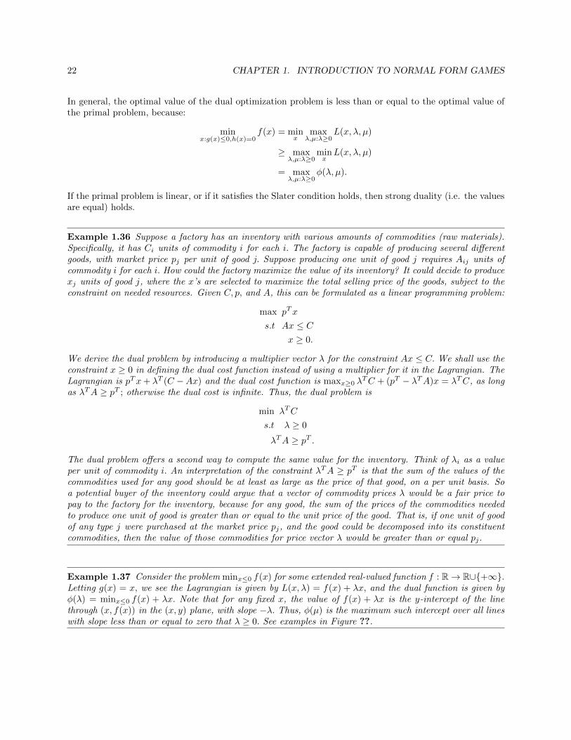
Example 1.36 Suppose a factory has an inventory with various amounts of commodities (raw materials).Specifically, it has Ci units of commodity i for each i. The factory is capable of producing several differentgoods, with market price pj per unit of good j. Suppose producing one unit of good j requires Aij units ofcommodity i for each i. How could the factory maximize the value of its inventory? It could decide to producexj units of good j, where the x’s are selected to maximize the total selling price of the goods, subject to theconstraint on needed resources. Given C, p, and A, this can be formulated as a linear programming problem:
max pTx
s.t Ax ≤ Cx ≥ 0.
We derive the dual problem by introducing a multiplier vector λ for the constraint Ax ≤ C. We shall use theconstraint x ≥ 0 in defining the dual cost function instead of using a multiplier for it in the Lagrangian. TheLagrangian is pTx+ λT (C −Ax) and the dual cost function is maxx≥0 λ
TC + (pT − λTA)x = λTC, as longas λTA ≥ pT ; otherwise the dual cost is infinite. Thus, the dual problem is
min λTC
s.t λ ≥ 0
λTA ≥ pT .
The dual problem offers a second way to compute the same value for the inventory. Think of λi as a valueper unit of commodity i. An interpretation of the constraint λTA ≥ pT is that the sum of the values of thecommodities used for any good should be at least as large as the price of that good, on a per unit basis. Soa potential buyer of the inventory could argue that a vector of commodity prices λ would be a fair price topay to the factory for the inventory, because for any good, the sum of the prices of the commodities neededto produce one unit of good is greater than or equal to the unit price of the good. That is, if one unit of goodof any type j were purchased at the market price pj, and the good could be decomposed into its constituentcommodities, then the value of those commodities for price vector λ would be greater than or equal pj .
Example 1.37 Consider the problem minx≤0 f(x) for some extended real-valued function f : R→ R∪+∞.Letting g(x) = x, we see the Lagrangian is given by L(x, λ) = f(x) + λx, and the dual function is given byφ(λ) = minx≤0 f(x) + λx. Note that for any fixed x, the value of f(x) + λx is the y-intercept of the linethrough (x, f(x)) in the (x, y) plane, with slope −λ. Thus, φ(µ) is the maximum such intercept over all lineswith slope less than or equal to zero that λ ≥ 0. See examples in Figure ??.

Chapter 2
Evolution as a Game
2.1 Evolutionarily stable strategies
Consider a population of individuals, where each individual is of some type. Suppose individuals haveoccasional pairwise encounters. During an encounter the two individuals involved play a two player symmetricgame in which the strategies are the types of the individuals. As a result of the encounter, each of the twoindividuals produces a number of offspring of its same type, with the number being determined by a fitnesstable or, equivalently, a fitness matrix. For example, consider a population of crickets such that each cricketis either small or large. If two small crickets meet each other then they each spawn five more small crickets.If a small cricket encounters a large cricket then the small cricket spawns one more small cricket and thelarge cricket spawns eight new large crickets. If two large crickets meet then each of them spawns three newlarge crickets. We can summarize these outcomes using the fitness matrix shown in Table 2.1.
Table 2.1: Fitness matrix for a population consisting of small and large crickets.
small largesmall 5, 5 1, 8large 8, 1 3, 3
or, for short, F =
(5 18 3
).
If a type i individual encounters a type j individual, then the type i individual spawns F(i,j) new individualsof type i, and the type j individual spawns F(j,i) new individuals of type j.
For example, consider a homogeneous population in which all individuals are of a single type S. Sup-pose a small number of individuals of type T is introduced into the population (or some individuals oftype T invade the population). If the T ’s were to replicate faster than the S’s they could change thecomposition of the population. For example, that is why conservationists are seeking to prevent an in-vasive species of fish from entering Lake Michigan http://www.chicagotribune.com/news/nationworld/
midwest/ct-asian-carp-lake-michigan-20170623-story.html. Roughly speaking, the type S is said tobe evolutionarily stable if S is not susceptible to such invasions, in the regime of very large populations.
Definition 2.1 (Evolutionarily stable pure strategies) A type S is an evolutionarily stable strategy (ESS) if
23

24 CHAPTER 2. EVOLUTION AS A GAME
for all ε > 0 sufficiently small, and any other type T,
(1− ε)F (S, S) + εF (S, T ) > (1− ε)F (T, S) + εF (T, T )
That is, if S is invaded by T at level ε then S has a strictly higher mean fitness level than T .
Note that the ESS property is determined entirely based on the fitness matrix; no explicit populationdynamics are involved in the definition.
Consider the large vs. small crickets example with fitness matrix given by Table 2.1. The large type is ESSby the following observations. For a population of large crickets with a level ε invasion of small crickets,the average fitness of a large cricket is 3(1 − ε) + 8ε = 3 + 5ε, while the average fitness of a small cricketis (1 − ε) + 5ε = 1 + 4ε. So the invading small crickets are less fit, suggesting their population will staysmall compared to the population of large crickets. In contrast, small is not ESS for this example. For apopulation of small crickets with a level ε invasion of large crickets, the average fitness of a small cricket is5(1− ε) + ε = 5− 4ε, while the average fitness of a large cricket is 8(1− ε) + 3ε = 8− 5ε. Thus, the averagefitness of the invading large crickets is greater than the average fitness of the small crickets. Note that forthe bi-matrix game specified in Table 2.1, large is a strictly dominant strategy (or type). In general, strictlydominant strategies are ESS and if there is a strictly dominant strategy, no other strategy can be ESS.
The definition of ESS can be extended to mixed strategies, as follows.
Definition 2.2 (Evolutionarily stable mixed strategies) A mixed strategy p∗ is an evolutionarily stable strat-egy (ESS) if there is an ε > 0 so that for any ε with 0 < ε ≤ ε and any mixed strategy p′ with p′ 6= p∗,
u(p∗, (1− ε)p∗ + εp′) > u(p′, (1− ε)p∗ + εp′). (2.1)
Proposition 2.3 (First characterization of ESS using Maynard Smith condition) p∗ is ESS if and only ifthere exists ε > 0 such that
u(p∗, p) > u(p, p) (2.2)
for all p with 0 < ‖p∗ − p‖1 ≤ 2ε. (By definition, ‖p∗ − p‖1 =∑a |p∗a − pa|.)
Proof. Before proving the if and only if portions separately, note the following. Given strategies p∗ and p′
and ε > 0, let p = (1 − ε)p∗ + εp′. Then u(p, p) = u((1 − ε)p∗ + εp′, p) = (1 − ε)u(p∗, p) + εu(p′, p), whichimplies that (2.1) and (2.2) are equivalent.
(if) (We can take ε and ε to be the same for this direction.) Suppose there exists ε > 0 so that (2.2) holdsfor all p with 0 < ‖p∗ − p‖1 ≤ 2ε. Let p′ be any strategy with p′ 6= p∗ and let ε satisfy 0 < ε ≤ ε. Letp = (1 − ε)p∗ + εp′. Then 0 < ‖p∗ − p‖1 ≤ 2ε so that (2.2) holds, which is equivalent to (2.1), so that p∗ isESS.
(only if) Suppose p∗ is ESS. Let ε be as in the definition of ESS so that (2.1) holds for any p′ 6= p∗ and anyε with 0 < ε ≤ ε. Let ε = εminp∗i : p∗i > 0. Let p be a mixed strategy such that 0 < ‖p∗ − p‖1 ≤ 2ε. Inparticular, |p∗i − pi| ≤ ε for all i. Then there exists a mixed strategy p′ such that p = (1− ε)p∗+ εp′ for some
p′ with p′ 6= p∗. Indeed, it must be that p′ = p−(1−ε)p∗ε . It is easy to check that the entries of p′ sum to one.
Furthermore, clearly p′i ≥ 0 if p∗i = 0. If p∗i > 0 then pi − (1 − ε)p∗i ≥ p∗i − ε − (1 − ε)p∗i = εp∗i − ε ≥ 0. Byassumption, (2.1) holds, which is equivalent to (2.2).

2.2. REPLICATOR DYNAMICS 25
Proposition 2.4 (Second characterization of ESS using Maynard Smith condition) p∗ is ESS if and only iffor every p′ 6= p∗, either
(i) u(p∗, p∗) > u(p′, p∗), or
(ii) u(p∗, p∗) = u(p′, p∗) and the Maynard Smith condition holds: u(p∗, p′) > u(p′, p′).
Proof. (only if) Suppose p∗ is an ESS. Since u(p, q) is linear in each argument, (2.2) is equivalent to
(1− ε)u(p∗, p∗) + εu(p∗, p′) > (1− ε)u(p′, p∗) + εu(p′, p′) (2.3)
so there exists ε > 0 so that (2.3) holds for all 0 < ε ≤ ε. Since the terms with factors (1 − ε) dominate asε→ 0, it follows that either (i) or (ii) holds.
(if) (The proof for this part is slightly complicated because in the definition of ESS, the choice of ε isindependent of p′.) Suppose either (i) or (ii) holds for every p′ 6= p∗. Then u(p∗, p∗) ≥ u(p′, p∗) for all p′.Let F = p′ : u(p∗, p∗) = u(p′, p∗) and let G = p′ : u(p∗, p′) > u(p′, p′). By the continuity of u, F is aclosed set and G is an open set, within the set of mixed strategies Σ. By assumption, F ⊂ G. The functionu(p∗, p∗) − u(p′, p∗) is strictly positive on F c and hence also on the compact set Gc = Σ\G. Since Gc isa compact set, the minimum of u(p∗, p) − u(p′, p∗) over Gc exists, and is strictly positive. The functionp′ 7→ u(p′, p′)− u(p∗, p∗) is a continuous function on the compact set Σ and is thus bounded below by somepossibly negative constant. So there exists ε > 0 such that
(1− ε) minu(p∗, p∗)− u(p′, p∗) : p′ ∈ Gc+ εminu(p∗, p′)− u(p′, p′) : p′ ∈ Σ > 0.
It follows that for any ε with 0 < ε ≤ ε, (2.3), and hence also (2.1), holds. Thus, p∗ is ESS.
The following is immediate from Proposition 2.4.
Corollary 2.5 (ESS and Nash equilibria) Consider a symmetric two-player normal form game.
(i) If a mixed strategy p is ESS then (p, p) is a Nash equilibrium.
(ii) If (p, p) is a strict Nash equilibrium in mixed strategies, then p is ESS.
2.2 Replicator dynamics
Continue to consider a symmetric two-player game with payoff functions u1 and u2. The symmetry meansS1 = S2 and for any strategy profile (x, y), u1(x, y) = u2(x, y), and u1(x, y) is the same as F (x, y), where Fis the fitness matrix. For brevity, we write u(x, y) instead of u1(x, y). Consider a large population such thateach individual in the population has a type in S1. Let ηt(a) denote the number of type a individuals at timet. We take ηt(a) to be a nonnegative real value, rather than an integer. Assuming it is a large real value
the difference is relatively small. Sometimes such models are called fluid models. Let θt(a) = ηt(a)∑a′ ηt(a
′) , so
that θa(t) is the fraction of individuals of type a. That is, if an individual were selected from the populationuniformly at random at time t, θt represents the probability distribution of the type of the individual. Recallthat, thinking of u as the payoff of player 1 in a normal form game, u(a, θt) is the expected payoff of player1 if player 2 uses the mixed strategy θt. In the context of evolutionary games, u(a, θt) is the average fitnessof an individual of type a for an encounter with another individual selected uniformly at random from the

26 CHAPTER 2. EVOLUTION AS A GAME
population. The (continuous time, deterministic) replicator dynamics is given by the following ordinarydifferential equation, known as the fitness equation:
ηt(a) = ηt(a)u(a, θt).
The fitness equation implies an equation for the fractions. Let Dt =∑a′ ηt(a
′) so that θt(a) = ηt(a)Dt
. By thefitness equation and the rule for derivatives of ratios,
θt(a) =ηt(a)Dt − ηt(a)Dt
D2t
=ηt(a)u(a, θt)
Dt−ηt(a)
∑a′ ηt(a
′)u(a′, θt)
D2t
which can be written as:
θt(a) = θt(a)(u(a, θt)− u(θt, θt)). (2.4)
The term u(θt, θt) in (2.4) is the average over the population of the average fitness of the population. Thus,the fraction of type a individuals increases if the fitness of that type against the population, namely u(a, θt),is greater than the average fitness of all types.
Let θ be a population share state vector for the replicator dynamics. That is, θ is a probability vector overthe finite set of types, S1. The following definition is standard in the theory of dynamical systems:
Definition 2.6 (Classification of states for the replicator dynamics)
(i) A vector θ is a steady state if θ
∣∣∣∣θ=θ
= 0.
(ii) A vector θ is a stable steady state if for any ε > 0 there exists a δ > 0 such that if ‖θ(0)− θ‖ ≤ δ then‖θ(t)− θ‖ ≤ δ for all t ≥ 0,
(iii) A vector θ is an asymptotically stable steady state if it is stable, and if for some η > 0, if ‖θ(0)− θ‖ ≤ ηthen limt→∞ θ(t) = θ.
Example 2.7 Consider the replicator dynamics for the Doves-Hawks game with the fitness matrix shown.Think of the doves and hawks as two types of birds that need to share resources, such as food. A dove has
Player 1
Player 2Dove Hawk
Dove 3,3 1,5Hawk 5,1 0,0
higher fitness, 3, against another dove than against a hawk, A hawk has a high fitness against a dove (5)but zero fitness against another hawk; perhaps the hawks fight over their resources. The two-dimensionalstate vector (θt(D), θt(H)) has only one degree of freedom because it is a probability vector. For brevity, letxt = θt(D), so θt = (xt, 1− xt). Observe that
ut(D, θt) = 3xt + (1− xt) = 2xt + 1
ut(H, θt) = 5xt
ut(θt, θt) = xt(2xt + 1) + (1− xt)(5xt) = 6xt − 3x2t

2.2. REPLICATOR DYNAMICS 27
So (2.4) gives
xt = xt(ut(D, θt)− ut(θt, θt))= xt(3x
2t − 4xt + 1)
= xt(1− xt)(1− 3xt). (2.5)
Sketching the right-hand side of (2.5) vs. xt and indicating the direction of flow of xt shows that 0 and 1are steady states for xt that are not stable, and 1
3 is an asymptotically stable point for xt. See Figure 2.1Consequently, (1, 0) and (0, 1) are steady states for θt that are not stable, and ( 1
3 ,23 ) is an asymptotically
10 1/3
Figure 2.1: Sketch of h(x) = x(1− x)(1− 3x) as both a function and one-dimensional vector field.
stable point for θt. In fact, if 0 < θ0(D) < 1 then θt → ( 13 ,
23 ) as t→∞.
Definition 2.8 (Trembling hand perfect equilibrium) A strategy vector (p1, . . . , pn) of mixed strategies for anormal form game is a trembling hand perfect equilibrium if there exists a sequence of fully mixed vectors ofstrategies p(n) such that p(n) → (p1, . . . , pn) and
pi ∈ Bi(p(n)−i ) for all i, n (2.6)
Remark 2.9 (i) The terminology “trembling hand” comes from the image of any other player j intendingto never use an action a such that pj(a) = 0, but due to some imprecision, the player uses the actionwith a vanishingly (as n→∞) small positive probability.
(i) The definition requires 2.6 to hold for some sequence p(n) → (p1, . . . , pn), not for every such sequence.
(i) Trembling hand perfect equilibrium is a stronger condition than Nash equilibrium; Nash equilibrium onlyrequires pi ∈ Bi(p−i) for all i.
Figure 2.2 gives a classification of stability properties of states for replicator dynamics based on a symmetrictwo-player matrix game. Perhaps the most interesting implication shown in Figure 2.2 is the topic of thefollowing proposition.
Proposition 2.10 If s is an evolutionarily stable equilibrium (ESS) then it is an asymptotically stable statefor the replicator dynamics.
Proof. Fix an ESS probability vector θ. We use Kulback-Leibler divergence as a Lyapunov function. Thatis, define V (θ) by
V (θ) = D(θ‖θ) ,∑
a:θ(a)>0
−θ(a) lnθ(a)
θ(a).
It is well known that D(θ‖θ) is nonnegative, jointly convex in (θ, θ), and D(θ‖θ) = 0 if and only if θ = θ.Therefore, V (θ) ≥ 0 with equality if and only if θ = θ. Also, V (θ) is finite and continuously differentiablefor θ sufficiently close to θ, because such condition ensures that θ(a) > 0 for all a such that θ(a) > 0.

28 CHAPTER 2. EVOLUTION AS A GAME
For brevity, write Vt = V (θ(t)). Then by the chain rule of differentiation, the replicator fitness equation, andProposition 2.3,
˙V = ∇V (θ(t)) · θt
= −∑
A:θ(a)>0
θ(a)
θt(a)θt(a)(u(a, θt)− u(θt, θt))
= −(u(θ, θt)− u(θt, θt))
< 0 for sufficiently small ‖θt − θ‖
Therefore θ is an asymptotically stable state.
Proposition 2.11 [2] If p is an asymptotically stable state of the replicator dynamics, then (p, p) is anisolated trembling hand perfect equilibrium of the underlying two-player game.
Example 2.12 Consider the replicator dynamics for the Dove-Robin-Owl game with the fitness matrixshown. The owls are strictly less fit than any other species, so the only equilibrium concept including the
Player 1
Player 2Dove Robin Owl
Dove 3,3 3,3 2,2Robin 3,3 3,3 1,1
Owl 2,2 1,1 0,0
owls is that a pure owl population, that is distribution (0, 0, 1), is a steady state of the replicator dynamics.
So consider the population distributions that do not include a positive fraction of owls. They are distributionsof the form (x, 1−x, 0). With no owls, the doves and robin populations grow in proportion, with the fractionsconstant. Thus (x, 1−x, 0) is a steady state for any x with 0 ≤ x ≤ 1. In fact, it is easy to check the strongerstatement: (x, 1− x, 0) is a Nash equilibrium for any x with 0 ≤ x ≤ 1.
If there is a small positive fraction of owl’s around then the dove’s have a slight advantage over the robins.Thus, only (1, 0, 0) is a trembling hand perfect equilibrium distribution. The fact (1, 0, 0) is easy to verifydirectly from the definition. The state (1, 0, 0) is not asymptotically stable because it is not an isolated stablestate. It follows that (1, 0, 0) is not an ESS either, which can also be checked using Proposition 2.4.
The only remaining question is which of the strategies of the form (x, 1−x, 0), if any, are stable steady statesof the replicator dynamic. A bit of analysis shows that they are all stable steady states. Indeed, if θ0 is closeto (x, 1−x, 0) and if there are initially no owls, then the initial state is a steady state so that θt is as close to(x, 1− x, 0) as the initial state is. If there is initally a small positive fraction of owls, since the fitness of theowls is dominated by the fitnesses of the other two types, the fraction of owls converges to zero exponentiallyquickly. Thus, while the dove’s get a small boost over the robins due to the owls, the effect converges to zeroas the initial fraction of owls converges to zero.
Additional reading
See [19, pp. 225-230] and [5, Chapter 7] for additional reading. The concept of trembling hand equilibriumplays a larger role in Chapter 4.

2.2. REPLICATOR DYNAMICS 29
s is a strictlydominant strategy
s is an asymptoticallystable state of replicatordynamics
s is an evolutionarilystable strategy (ESS)
s is a steady stateof replicator dynamics
(s, s) is an NE
(s, s) is a strict NE
(s, s) is a tremblinghand perfect equilibrium
s is a stablesteady state ofreplicator dynamics
defn
defn
defn
defn
Lyapunov
argument
SeeShoav Leyton-Browntextforreferences
Figure 2.2: Classification of states, for evolution based on a symmetric two-person normal form game. Thethree definitions in the shaded box involve the replicator dynamics; the other definitions only implicitlyinvolve dynamics.

30 CHAPTER 2. EVOLUTION AS A GAME
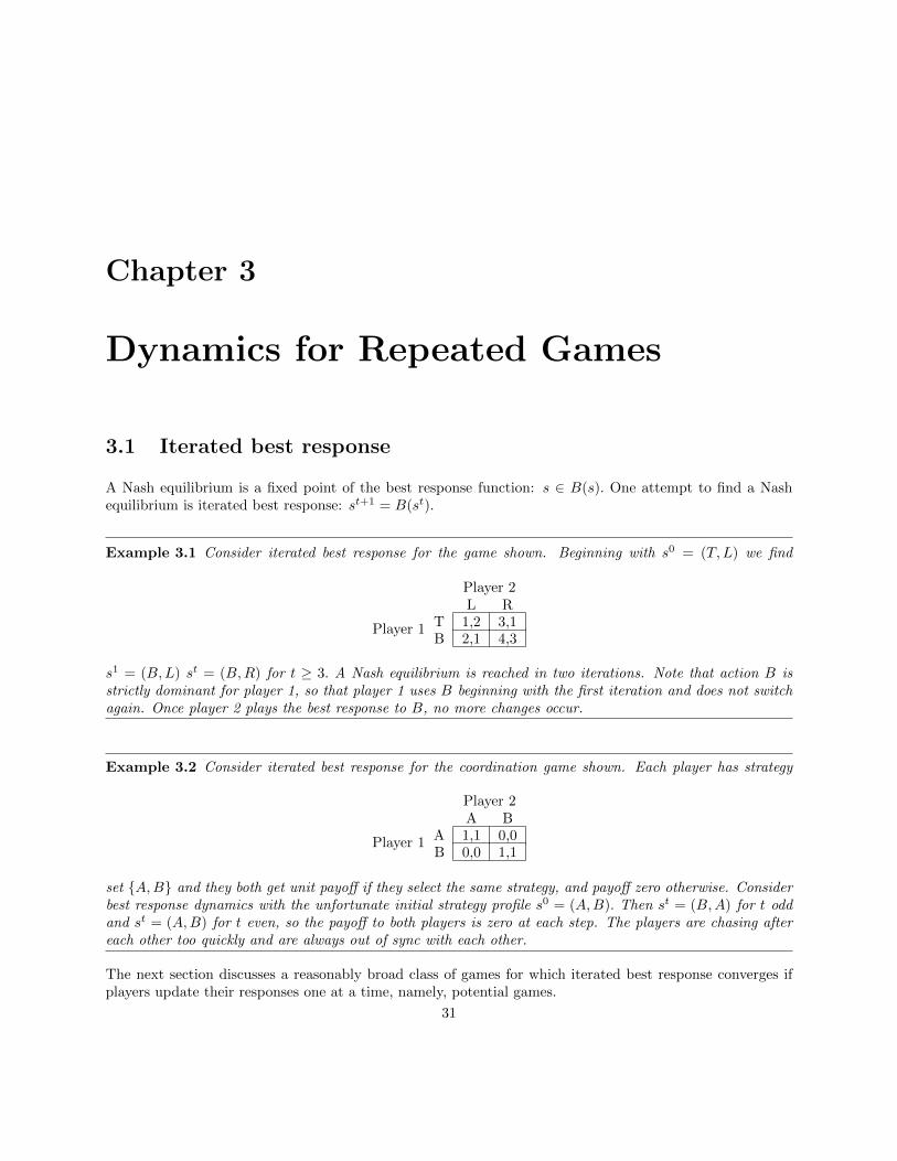
Chapter 3
Dynamics for Repeated Games
3.1 Iterated best response
A Nash equilibrium is a fixed point of the best response function: s ∈ B(s). One attempt to find a Nashequilibrium is iterated best response: st+1 = B(st).
Example 3.1 Consider iterated best response for the game shown. Beginning with s0 = (T, L) we find
Player 1
Player 2L R
T 1,2 3,1B 2,1 4,3
s1 = (B,L) st = (B,R) for t ≥ 3. A Nash equilibrium is reached in two iterations. Note that action B isstrictly dominant for player 1, so that player 1 uses B beginning with the first iteration and does not switchagain. Once player 2 plays the best response to B, no more changes occur.
Example 3.2 Consider iterated best response for the coordination game shown. Each player has strategy
Player 1
Player 2A B
A 1,1 0,0B 0,0 1,1
set A,B and they both get unit payoff if they select the same strategy, and payoff zero otherwise. Considerbest response dynamics with the unfortunate initial strategy profile s0 = (A,B). Then st = (B,A) for t oddand st = (A,B) for t even, so the payoff to both players is zero at each step. The players are chasing aftereach other too quickly and are always out of sync with each other.
The next section discusses a reasonably broad class of games for which iterated best response converges ifplayers update their responses one at a time, namely, potential games.
31

32 CHAPTER 3. DYNAMICS FOR REPEATED GAMES
3.2 Potential games
(Monderer and Shapley, [12])
Let G = (I, (Si), (ui)) be an n-player normal form game and let S =×i∈I Si denote the product space ofaction vectors.
Definition 3.3 A potential function for G is a function Φ : S 7→ R such that
ui(x, s−i)− ui(y, s−i) = Φ(x, s−i)− Φ(y, s−i)
for all i ∈ I and all x, y in Si and s−i ∈ S−i. (Here, S−i =×N
i′∈I\i Si′ .)
Note that if G has a potential function Φ and if the action of a single player i changes, there is no restrictionon the change of payoff functions of the other players. If a game has a potential function it is easy to findone, because for any two s, s′ ∈ S, the difference Φ(s)−Φ(s′) can be found by changing the coordinates of sinto coordinates of s′ one at a time. The order the coordinates are changed in must give the same difference,which is why the property of having a potential function is a rather special property of a game. If Φ is apotential function, then so is Φ + c for a constant c, so in searching for a potential function we can assignan arbitrary real value to Φ(s) for one strategy profile vector s ∈ S.
Example 3.4 Recall the prisoner’s dilema. Let us seek a potential function Φ. We can set Φ(C,C) = 0
Player 1
Player 2C (cooperate) D
C (cooperate) 1,1 -1,2D 2,-1 0,0
without loss of generality. If the action of either player is changed from C to D then the payoff of thatplayer increases by one, so Φ(C,D) = Φ(D,C) = 1. Starting with (D,C), if the action of player 2 changesto D, then the payoff of player 2 again increases by one, so it must be that Φ(D,D) = 2. Thus, if there is apotential function, then following table must give the function. Checking all cases we can verify that indeed,the game is a potential game and the potential function is given by
Player 1
Player 2C (cooperate) D
C (cooperate) Φ = 0 Φ = 1D Φ = 1 Φ = 2
In a homework problem we address the following question: Does every symmetric two player game have apotential function?
The proof of the following proposition is simple and is left to the reader.
Proposition 3.5 Suppose G has a potential Φ.
(i) For s ∈ S, s is a pure strategy Nash equilibrium (NE) if and only if s is a local maximum of Φ (wherethe neighbors of s are strategy profiles obtained by changing the strategy for a single player).
(ii) If G is a finite game (meaning that all action sets are finite) then arg max Φ 6= ∅ and there existsat least one pure Nash equilibrium. Furthermore, if s0 is an arbitrary strategy vector and a sequences0, s1, . . . of strategy vectors is determined by using single player better response dynamics (players

3.2. POTENTIAL GAMES 33
consider whether to change strategies one at a time and any time a player can change strategies tostrictly increase the payoff of the player, some such change is made), then the sequence terminatesafter a finite number of steps and ends at a NE.
Example 3.6 (Single resource congestion game) Suppose there is some resource that can be shared, such asa swimming pool. Each player makes a binary decision, so that si ∈ Si = 0, 1 for each i, where si = 1denotes that player i will participate in sharing the resource. The total number of players participating is|s| , s1 + . . . + s|I|. Suppose the payoff of a player is zero if the player does not participate, and the payoffis v(k) if a total of k players participate, where v : 0, . . . , |I| 7→ R. That is, ui(s) = siv(|s|). Thus, v(k)represents the value of participating for a player given that a total of k players are participating. Some valuesof v could be negative. In many applications, v(k) is decreasing in k, for example representing a fixed rewardfor participating minus a congestion cost that increases with the number of participants. Is this a potentialgame?Solution: Let us seek a potential function Φ. By definition, a function Φ is a potential function if and onlyif it satisfies
ui(1, s−i)− ui(0, s−i) = Φ(1, s−i)− Φ(0, s−i)
for any player i and any s−1 ∈ S−i. If s−i has k ones, this becomes
v(k + 1)− 0 = Φ(1, s−i)− Φ(0, s−i).
That is because, if k other players are participating, if another player decides to participate, the payoff ofthat player goes from 0 to v(k + 1). Here, (1, s−i) and (0, s−i) can represent an arbitrary pair of strategyprofiles such that |s| = k + 1 and |s′| = k. Thus, it must be that Φ(s) = Φ(0) + v(1) + · · · + v(|s|) for anys 6= (0, . . . , 0).
As a slight generalization of this example, a player dependent participation price pi can be incorporated togive ui(s) = si(v(|s|)− pi), with the corresponding potential Φ(s) = v(1) + · · ·+ v(|s|)−
∑i∈I sipi.
Example 3.7 (Multiple resource congestion game) We can extend the previous example to a set L of L ≥ 1resources. Each resource can be shared by a number of players. Each player i can select a bundle of resourcessi to participate in sharing, such that the bundle for player i is required to be chosen from some set of bundlesSi. That is, si ∈ Si and si ⊂ L, and Si is a nonempty set of subsets of L. For example, the resources couldrepresent communication links or transportation links in a graph, and a bundle of resources could representa path through the graph or a set of paths through the graph. The payoff functions are given by:
ui(si, s−i) = Ri(si) +∑`∈si
v`(k`)
where
• Ri : Si → R for each player i,
• k` for each ` is the number of players using resource ` (i.e. number of i with ` ∈ si.)
• v` : 0, . . . , |I| → R for each ` ∈ L,

34 CHAPTER 3. DYNAMICS FOR REPEATED GAMES
The same reasoning used in Example 3.6 shows that this is a potential game for the potential function
Φ(s) =∑i
Ri(si) +∑`∈L
∑k:1≤k≤k`
v`(k).
There are not many practical examples of potential games beyond congestion games. However, Proposition3.5 holds for games that have an ordinal potential function, defined as follows.
Definition 3.8 (Monderer and Shapley, [12]) A function Φ : S → R is an ordinal potential function for agame G = (I, (Si), (ui)) if
ui(s′i, s−i) > ui(si, s−i) if and only if Φ(s′i, s−i) > Φ(si, s−i)
for all i ∈ I and all s = (si, s−i) ∈ S and s′i ∈ Si.
Example 3.9 (Cournot competition) Suppose there is a single commodity, such as sugar, and a finite setof players that are firms that can produce the commodity. The action of each player i ∈ I is qi ∈ (0,∞),where qi denotes the quantity of the commodity player i will produce. The total amount of quantity producedis given by Q = q1 + · · · + qI . Suppose that the demand for the quantity is such that all the commoditywill be consumed for any Q > 0 with the market price per unit quantity equal to P (Q) for some functionP : (0,∞) → (0,∞). Suppose the production cost per unit commodity is C for each player, where C > 0.Then the payoff function of player i is defined by:
u(qi, q−i) = qi(P (Q)− C)
So the payoff is the quantity produced by firm i times the price per unit production minus the cost per unitproduction. We could make this a finite game by restricting the quantity qi to be selected from some finitenonempty subset Si of (0,∞) for each i. It is easy to check that the following specifies an ordinal potentialfunction Φ for this game:
Φ(q) =
∏j∈I
qj
(P (Q)− C) .
3.3 Fictitious play
A similar but smoother algorithm than iterated best response is fictitious play. In iterated best response,each player gives the best response to the most recent play of the other players. In fictitious play, eachplayer gives a best response to the empirical distributions of all past plays of the other players. To describefictitious play we use the following notation. Fix a finite n-player normal form game (I, (Si)i∈I , (ui)i∈I).
• Let st = (sti)i∈I denote the strategy profile used at time t for integer t ≥ 1. Although we assume theplayers select pure strategies at each time, we write sti as a 0-1 probability vector. For example, if Sihas four elements that are indexed by 1 through 4, then sti = (0, 1, 0, 0) indicates that player i selectsthe second action from Si at the tth play of the game.
• Let nti(a) denote the number of times player i played action a up to time t. Set nti = (nti(a))a∈Si .

3.3. FICTITIOUS PLAY 35
• To get an initial state, suppose to is a positive integer and suppose for each player i that (n0i (a) : a ∈ Si)
is a vector of nonnegative integers with sum to. Pretend the game was played t0 times up to time 0and that n0
i (a) is the number of times player i selected strategy a up to time 0.
• Let µti =(nti(a)to+t
)a∈Si
, for t ≥ 0, which is the empirical probability distribution of the actions taken by
player i up to time t, including the to pretend actions.
• Let µt = (µt1, . . . , µtn) be the tuple of empirical probability distributions of strategies used by all players,
observed in play up to time t.
Since nt+1i = nti + st+1
i for t ≥ 0, we have the following update equation for the empirical distributions:
µt+1i =
nt+1i
t+ to + 1=nti + st+1
i
t+ to + 1
= µti + αt(st+1i − µti),
where αt = 1t+to+1 . The fictitious play algorithm is given by
st+1i ∈ Bi(µt−i) (3.1)
µt+1i = µti + αt(s
t+1i − µti), (3.2)
where αt = 1t+to+1 . Equation (3.1) indicates that player i is selecting a best response at time t+ 1 as if the
other players each use a mixed strategy with probability distribution equal to the empirical distribution oftheir past actions, and (3.2) simply updates the empirical distribution of past plays.
Proposition 3.10 Suppose the fictitious play algorithm (3.2) - (3.1) is run and suppose the vector of em-pirical distributions converges: µt → σ as t → ∞ for some mixed strategy profile σ. Then σ is a Nashequilibrium.
Proof. Suppose µt → σ as t→∞. Then σ is a mixed strategy profile for the game because pointwise limitsof probability vectors over finite action sets are probability vectors. It remains to show that σ is a Nashequilibrium. Focus on any player i and let a ∈ Si such that a 6∈ Bi(σ−i). It suffices to show that σi(a) = 0.By the assumption µt → σ it follows that a 6∈ B(µt−i) for all sufficiently large t. Therefore, sti(a) = 0 for allsufficiently large t., which implies nti stops increasing for large enough t. Therefore, σi(a) = limt→∞ µti(a) = 0.
So the good news about fictitious play is that if the empirical distribution converges then the limit is a Nashequilibrium. The bad news is that the empirical distribution might not converge, and even if it does, theNash equilibrium found might not be a very desirable one.
Example 3.11 (Fictitious play for the coordination game) Consider the coordination game of Example 3.2.To be definite, suppose in the case of a tie for best response actions, that a best response action is selectedat random with each possibility having positive probability bounded away from zero for all time. Considerthe reasonable initial state to = 2 and n0
i = (1, 1) for both players. That is, pretend that up to time zeroeach player selected each action one time. Then for the initial selection at time 1, either response for eitherplayer i is a best response to µ0
−i. If the players are lucky and they both select the same strategy, then theywill forever continue to select the same strategy, and their payoffs will both be one for every play. Moreover,

36 CHAPTER 3. DYNAMICS FOR REPEATED GAMES
the empirical distribution will converge to one of the two Nash equilibria in pure strategies, correspondingto (A,A) or (B,B). If they are unlucky at t = 1 and player 1 selects A and player 2 selects B, thenµ1 = ((2/3, 1/3), (1/3, 2/3)). So for t = 2, player 1 selects the best response for distribution (1/3,2/3) forplayer 2, which is action B, or as a mixed strategy, action (0, 1). Similarly, player 2 selections action A,or (1, 0) and the payoffs are both zero at tine t = 2. Then the empirical distribution after two steps isµ2 = ((2/4, 2/4), (2/4, 2/4)), which is again a tie. Whenever there is such a tie the two players could againbe unlucky and suffer two more rounds of zero payoff. However, with probability one they will eventuallyselect the same actions when in a tied state, and from then on they will receive payoff 1 every time and theempirical distribution will converge to one of the two pure strategy equilibriums.
However, consider a variation such that in case of a tie, player 1 selects action A, and in case of a tie,player 2 selects action B. Then from the same initial state as before the sequence of strategy profiles willbe st = (A,B) for t odd and st = (B,A) for t even, and the payoffs of both players are zero for all plays.The empirical distributions of plays converges for both players, with the limit of empirical distribution profilegiven by limt→∞ µt = σ = ((0.5, 0.5), (0.5, 0.5)). Notice that σ is indeed a mixed strategy Nash equilibrium asguaranteed by Proposition 3.10, but the payoffs of both players is only 0.5.
Example 3.12 (Fictitious play for Shapley’s modified rock scissors paper) Consider the variation of rockscissors paper such that the payoff of the loser is 0 instead of -1, giving the following payoff matrix: This
Player 1
Player 2R S P
R 0,0 1,0 0,1S 0,1 0,0 1,0P 1,0 0,1 0,0
is no longer a zero sum game. It has some aspect of the coordination game in it because the sum of payoffsis maximized (equal to one) if the players manage to select different actions. The algorithm is arbitrarily
t st1 st2 nt1 nt21 R S (1,0,0) (0,1,0)2 R P (2,0,0) (0,1,1)3 R P (3,0,0) (0,1,2)4 S P (3,1,0) (0,1,3)5 S P (3,2,0) (0,1,4)6 S P (3,3,0) (0,1,5)7 S P (3,4,0) (0,1,6)8 S R (3,5,0) (1,1,6)9 S R (3,6,0) (2,1,6)10 S R (3,7,0) (3,1,6)11 S R (3,8,0) (4,1,6)12 S R (3,9,0) (5,1,6)13 S R (3,10,0) (6,1,6)14 S R (3,11,0) (7,1,6)15 P R (3,11,1) (8,1,6)...
......
......

3.4. REGULARIZED FICTITIOUS PLAY AND ODE ANALYSIS 37
initialized to (R,S) for the first round of play. Player 1 continues to play R at t = 2 and t = 3 becauseof the initial play S by player 2. Player 2 switches to P at t = 2 and stays there awhile, as player 1 keepsplaying rock. Eventually player 1 switches to S is response to the large string of P by player 2. Player 2later switches to R because of the long string os S by player 1. And so forth. Each player moves from alosing action to a winning action, eventually causing the other player’s action to become losing, and then theother player changes actions, and the process continues. The empirical distribution does not converge forfictitious play in this example.
The payoff sequence is good – the sum of payoffs is always the maximum possible value, namely one.
Remark 3.13 Fictitious play is pretty difficult to analyze, but it does converge for the following special casesof two player games: (a) zero sum games, (b) common interest games with randomization at ties, (c) gamessuch that at least one player has at most two actions, with randomization at ties. See [18] for references.
Remark 3.14 The examples consider only two players. For three or more players we could have a playerrespond to either the strategy profile composed of the empirical distributions of each of the other players, orto the empirical distribution of the joint past plays of the other players.
3.4 Regularized fictitious play and ode analysis
The fictitious play algorithm given by (3.1) and (3.2) is difficult to analyze because the best response setBi(µ
t−i) can have more than one element, so we have a difference inclusion rather than a difference equation.
Also, the set Bi(µt−i) is not continuous in µt−i. We use a regularization technique to perturb the dynamics
to address both of those problems. This section is largely based on [18]. Probability distributions are takento be column vectors.
3.4.1 A bit of technical background
The entropy of a discrete probability distribution p is H(p) ,∑ni=1−pi ln pi, with the convention that
0 ln 0 = 0. The entropy of a distribution on a finite set is bounded: 0 ≤ H(p) ≤ lnn. Larger values ofentropy indicate the distribution is more spread out. H(p) = 0 if and only if p is a degenerate probabilitydistribution, concentrated on a single outcome. The mapping p 7→ H(p) is concave.
The Kullback-Liebler (KL) divergence between discrete probability distributions p and q is defined by
D(p‖q) =∑i
pi lnpiqi,
with the convention that 0 ln 0 = 0 ln 00 = 0. Values of the KL divergence range over 0 ≤ D(p‖q) ≤ +∞,
with D(p‖q) = 0 if and only if p = q. The mapping (p, q) 7→ D(p‖q) is jointly convex.
Let σ : Rm → R be defined by σ(r) = σ(r1, . . . , rm) =(
er1
er1+···+erm , · · · ,erm
er1+···+erm
)T. Also, define F :
Rm → R by F (r) = τ ln(∑m
a=1 era/τ
), where τ > 0 is a regularization parameter. F satisfies limτ→0 F (r) =
maxa ra for each r and ∇F (r) = σ(r/τ). For small τ > 0, F (r) approximates the maximum of r, and σ(r/τ)approximates the probability distribution uniformly distributed over the set of indices a that maximize ra.

38 CHAPTER 3. DYNAMICS FOR REPEATED GAMES
3.4.2 Regularized fictitious play for one player
Consider the special case of fictitious play as described in Section 3.3 for a game with only one player,namely, player 1. Equivalently, there could be other players in the game, but they always play the sameactions, so the payoff function for player 1 in each round is a time invariant function of the action chosenby player 1. Write the payoff function for player 1 as u1(a) = ra for a ∈ S1, so ra is the payoff, or reward,to player 1 for selecting action a. View r as a column vector. The set of mixed strategy best responses forplayer 1 is B1 = arg maxp∈Σ1
pT r, where Σ1 is the set of probability distributions on S1. The set B1 does notdepend on time because the payoff function does not depend on time. It is equal to the set of probabilitydistributions over S1 supported on the subset arg mina ra. The set B1 can have more than one element andwe didn’t specify a probability distribution over B1, and the set B1 is not a continuous function of r (whichwould be a problem if r is changing with time, as it will in the case of more than one player).
To obtain more tractable performance consider the following regularized payoff for player 1: u1(p) = pT r +τH(p), where H(p) is the entropy of p and τ > 0 is a regularization parameter. The best response for player1 in mixed strategies is now uniquely given by the following continuous function of r:
β(r) , arg maxp
pT r + τH(p)
= σ
( rτ
),
and for that distribution, the maximum payoff is F (r) = τ ln∑a e
ra/τ , where σ and F are defined in Section3.4.1. Using this regularization, the best response dynamics of (3.1) and (3.2) for player 1 reduces to thefollowing discrete time randomized algorithm to be executed at each t ≥ 0 :
select At+1 ∈ S1 with probability distribution β(r) (3.3)
µt+11 = µtt + αt(1At+1 − µ
ti) (3.4)
where αt = 1t+to+1 , and 1At+1 denotes the probability distribution on S1 with unit mass at At+1. Equation
(3.4) can be written as
µt+11 = µtt + αt(β(r)− µti) +Dt+1 (3.5)
where Dt+1 = 1At+1 − β(r). By (3.3), the random vector Dt is mean zero – in fact (Dt)t≥0 is a boundedmartingale difference sequence. By the theory of stochastic approximation, any limit point of (µt1) is in theset of fixed points for the ordinary differential equation (ode):
µ1 = αt(β(r)− µ1). (3.6)
The factor αt in the ode (3.6) can be eliminated by nonlinearly rescaling time. Specifically, let q be a solutionto the following ode:
q(t) = β(r)− q(t), (3.7)
Then µ1(t) = q(∫ t
0αsds
)is a solution to (3.6). In summary, (3.7) represents the ode approximation of
fictitious play dynamics for one player, with time rescaling to eliminate αt. We turn next to the analysis of(3.7).
The ode (3.7) is a simple linear ode, with solution given by q(t) = β(r) + (q(0) − β(r))e−t. This directlyproves limt→∞ q(t) = β(r). Let’s prove the same thing without solving for q, using the Lyapunov functionV (q) = F (r)− qr − τH(q). This choice of V is motivated by the fact q 7→ qr + τH(q) is the payoff functionfor player 1 seeks to maximize, and to get V (q) the payoff is subtracted from the maximum possible payoff,

3.4. REGULARIZED FICTITIOUS PLAY AND ODE ANALYSIS 39
F (r), which is achieved uniquely by q = β(r). In particular, V (q) ≥ 0 and V (q) = 0 if and only if q = β(r).Check that
∇V (q) = −r + τ
1 + ln q1
...1 + ln qn
.
Let Vt = V (q(t)). Check that˙Vt = −Vt−D(β(r)‖q(t)), whereD(·‖·) is the KL divergence function. Therefore,
˙V t ≤ −Vt. Thus, Vt ≤ V0e−t, implying that limt→∞ q(t) = β(r).
3.4.3 Regularized fictitious play for two players
Consider the two-player game in mixed strategies with payoff functions:
ui(qi, q−i) = qTi Miq−i + τH(qi)
If τ = 0 this game corresponds to the game in mixed strategies for the bimatrix game with payoff matrixMi for each player i. We consider τ > 0 that is small, acting as a regularizer.
The situation faced by each player i is similar to that faced by the single player in Section 3.4.2, but with rreplaced by Miq−i, which is a vector that can be time varying due to variation of the strategy of the otherplayer. In particular, the best response for player i for a fixed distribution q−i chosen by the other player is
βi(q−i) = σ(Miq−iτ
). This gives rise to the following ode model for continuous time fictitious play:
q1(t) = β1(q2(t))− q1(t) (3.8)
q2(t) = β2(q1(t))− q2(t). (3.9)
Equations (3.8) and (3.9) can be derived from discrete time models using the theory of stochastic approxi-mation in the same way (3.7) was derived.
To study convergence we consider Lyapunov functions similar to the one in Section 3.4.2.
V1(q1, q2) = F (M1q2)− u1(q1, q2)
V2(q1, q2) = F (M2q1)− u2(q1, q2)
V12(q1, q2) = V1(q1, q2) + V2(q1, q2)
Let Vi = Vi(q1(t), q2(t)) for i ∈ 1, 2 and V12 = V12(q1(t), q2(t)). It is shown below that:
˙V 1 ≤ −V1 + qT1 M1q2 (3.10)
˙V 2 ≤ −V2 + qT2 M1q1 (3.11)
For zero sum games, M2 = −MT1 so that qT1 M1q2 + qT2 M2q1 ≡ 0. Thus, with V12 = V1 + V2, in the case of
zero zero sum games,˙V 12 ≤ −V12 so that V (t) ≤ V (0)e−t so that V12(t)→ 0 as t→∞.
Proposition 3.15 If M2 = −MT1 (zero sum game) then any limit point of (q1, q2) is a Nash equilibrium.
Any isolated Nash equilibrium point is asymptotically stable.

40 CHAPTER 3. DYNAMICS FOR REPEATED GAMES
Proof. The proposition follows from the fact limt→∞˙V 12 = 0, which will be established once we prove
(3.10) and (3.11). By the calculations from Section 3.4.2,
∇qiVi(qi(t), q−i(t))T qi ≤ −Vi(qi(t), q−i(t))
By the fact ∇F (q) = σ(q/τ), we find
∇q−iVi(qi(t), q−i(t)) = ∇F (Miq−i)TMi −∇q−iui(q1, q2)
= (βi(q−i)− qi)TMi = qiTMi
so that ∇q−iVi(qi(t), q−i(t))qi = qiMiqi−1. Thus,
˙V 1 = ∇qiVi(qi(t), q−i(t))T qi +∇q−iVi(qi(t), q−i(t))T q−i ≤ −Vi + qTi Miq−i,
as was to be proved.
3.5 Prediction with Expert Advice
(Goes back to Hannan and Wald, among others. See [4])
3.5.1 Deterministic guarantees
Suppose a forecaster selects a prediction pt ∈ D of some outcome yt ∈ Y for each t ≥ 1. For a loss function` : D × Y → R, the cumulative loss of the forecaster up to time n is given by:
Ln =
n∑t=1
`(pt, yt)
The sequence y1, y2, . . . can be arbitrary. It might be that each outcome yt is given by a function of pastand present predictions and past outcomes, or it can be thought of as being selected arbitrarily by natureor by an adversary.
An interesting approach to this problem is based on the assumption that there are some experts, and theforecaster tries to do as well as any of the experts. Suppose there are N experts and expert i makes predictionfi,t ∈ D at time t. The cumulative loss for expert i is given by Li,n ,
∑nt=1 `(fi,t, yt) for i ∈ [N ]. The regret
of the forecaster for not following expert i is defined by:
Ri,n , Ln − Li,n =
n∑t=1
`(pt, yt)− `(fi,t, yt)︸ ︷︷ ︸ri,t
,
where the ith term of the sum is the instantaneous regret, ri,t. A reasonable goal for the forecaster is toperform, averaged over time, as well as any of the experts. The average regret per unit time converges tozero if
max1≤i≤N
1
n(Ln − Li,n)
n→∞−→ 0.

3.5. PREDICTION WITH EXPERT ADVICE 41
A desirable property for a forecaster would be to satisfy a universal performance guarantee: the averageregret per unit time converges to zero for an arbitrary choice of the y’s and arbitrary sequences of theexperts. We’ll see such forecasters exist if `(p, y) is a bounded function that is a convex function of p forfixed y. The following lemma is a key to the construction.
Lemma 3.16 Suppose `(p, y) is convex in p. For any nonzero weight vector (w1,t−1, . . . , wn,t−1) with non-negative entries, if
pt =
∑i wi,t−1fi,tDt−1
where Dt−1 =∑i′
wi′,t−1 (3.12)
then ∑i
wi,t−1ri,t ≤ 0
for any yt, where ri,t = `(pt, yt)− `(fi,t, yt).
Proof. For any yt,
`(pt, yt) = `
(∑i
wi,t−1
Dt−1fi,t, yt
)(a)
≤∑i
wi,t−1
Dt−1`(fi,t, yt) (3.13)
where (a) follows by Jensen’s inequality. The average of a constant is the constant, so
`(pt, yt) =∑i
wi,t−1
Dt−1`(pt, yt). (3.14)
Subtracting each side of (3.13) from the respective sides of (3.14) and cancelling the positive factor Dt−1
yields the lemma.
Lemma 3.16 shows that if the forecaster’s prediction is a convex combination of the predictions of the experts,then the forecaster’s loss will be less than or equal to the convex combination of the losses of the experts,formed using the same weights for both convex combinations. For example, if the forecaster uses the sameaction as one particular expert, then the loss of the forecaster will be no larger than the loss of that expert.If the forecaster simply uses the unweighted average of the actions of two particular experts, then the loss ofthe forecaster will be less than or equal to the unweighted average of the losses of those two experts. In orderto do well in the long run, the forecaster needs to put more weight on the more successful experts, which arethe ones giving the largest regret. One strategy would be to put all the weight on a single leading expert,but due to the arbitrary nature of the outcome sequence (yt), the forecaster is better off putting significantweight on experts doing nearly as well as the leading expert, as implied by the following example.
Example 3.17 Suppose D = [0, 1], Y = 0, 1, and `(p, y) = |p − y|. Suppose N = 2 with f1,t = 0 forall t and f2,t = 1 for all t. If the forecaster always follows a leading expert, then for each t, pt ∈ 0, 1 isone of the endpoints of D for each t. But then it is possible for the forecaster to be so unlucky as to havemaximum loss every time. That is, it could happen that yt = 1 whenever pt = 0 and yt = 0 whenever pt = 1,resulting in the largest possible loss for the forecaster at every time, yielding Ln = n for all n ≥ 1. A better

42 CHAPTER 3. DYNAMICS FOR REPEATED GAMES
strategy would be to select pt ≡ 1/2. Then Ln ≤ n2 for all n ≥ 1. How do the experts do for this example?
At each time, one of the two experts is correct and the other is not, so L1,n + L2,n = n for all n ≥ 1, sominL1,n, L2,n ≤ n
2 .
Given η > 0, let Φ : RN → RN be defined by1
Φ(x1, . . . , xN ) =1
ηln
N∑i=1
eηxi .
For large η, Φ is a version of soft max function; limη→∞Φ(x1, . . . , xN ) = maxx1, . . . , xN. In general,maxx1, . . . , xN ≤ Φ(x1, . . . , xN ) ≤ maxx1, . . . , xN+ lnN
η . The gradient of Φ is given by
∇Φ(x) =
eηx1
D(x)
...eηxND(x)
(3.15)
where D(x) =∑i′ e
ηxi′ . Thus, ∇Φ(x) is the transpose of a probability vector with most of the weight onthe indices of maximum value. That is, ∇Φ(x) is a soft max selector function. The function Φ is convex –in fact the sum of log convex functions is convex in general. A way to directly verify the convexity of Φ isto note that the Hessian matrix is given by
H(Φ)
∣∣∣∣x
=
(∂2H(Φ)
∂x1∂xj
)i,j
= η
(diag
(eηxi
D
)−(
eηxi
D
eηxj
D
)i,j
)(3.16)
Therefore, the Hessian matrix is symmetric and diagonal dominant, so it is positive definite.
Since the forecaster seeks to minimize the maximum regret over the N experts, we focus on the soft maximumregret, given by Φ(R1,t, . . . RN,t).
Let Rt = (R1,t, . . . , RN,t) and rt = (r1,t, . . . , rN,t). Note that Rt = Rt−1 + rt for t ≥ 1. By the intermediatevalue form of Taylor’s theorem,
Φ(Rt) = Φ(Rt−1 + rt)
= Φ(Rt−1) + 〈∇Φ(Rt−1), rt〉+1
2rTt H(Φ)
∣∣∣∣ξ
rTt (3.17)
for some ξ ∈ RN on the line segment with endpoints Rt−1 and Rt. The second term on the righthandside of (3.17) is a convex combination of the instantaneous regrets for different experts. In view of Lemma3.16, this suggests that the forecaster use (∇Φ(Rt−1))T as the weight vector on the experts, to ensure that〈∇Φ(Rt−1), rt〉 ≤ 0. That is, in view of (3.15), suppose the forecaster uses the strategy (3.12) for the weights:
wi,t−1 = eηRi,t−1 (3.18)
Lemma 3.16 implies that no matter what the values of f1,t, . . . , fN,t and yt are, 〈∇Φ(Rt−1), rt〉 = 〈pt, rt〉 ≤ 0.Since multiplying all the weights in (3.12) by the same constant does not change pt, the same sequence forthe predictor is generated by
wi,t−1 = e−ηLi,t−1 (3.19)
1Φ and η here are the same as F and 1/τ in Section 3.4.1.

3.5. PREDICTION WITH EXPERT ADVICE 43
With this choice of weights, as already mentioned, 〈∇Φ(Rt−1), rt〉 ≤ 0. So we next examine the last term onthe righthand side of (3.17).
Suppose the loss function is bounded. For convenience, assume it takes values in [0, 1]: `(p, y) ∈ [0, 1] for allp and y. Therefore, |ri,t| ≤ 1 for all i ∈ [N ] and t ≥ 1. This assumption and the expression (3.16) show that
rTt H(Φ)
∣∣∣∣ξ
rTt ≤ ηN∑i=1
eηξi
Dr2i,t ≤ η
N∑i=1
eηξi
D= η.
That is, the last term on the righthand side of (3.17) is less than or equal to η2 . Thus, (3.17) and the
assumptions made imply Φ(Rn) ≤ Φ(Rn−1) + η2 for all n ≥ 1. Since R0 ≡ 0, Φ(R0) = lnN
η . Therefore,
maxiRi,n ≤ Φ(Rn) ≤ nη2 + lnN
η . We thus have the following proposition.
Proposition 3.18 (Maximum regret bound for exponentially weighted forecaster, fixed time horizon) LetD and Y be nonempty sets such that D is convex, and let ` : D × Y → [0, 1] be such that p 7→ `(p, y) isconvex for any y fixed. For some n ≥ 1 let ((fi,t)1≤t≤n)i∈[N ] represent arbitrary strategies of N expertsand let (yt)1≤t≤n be an arbitrary outcome sequence. If the forecaster uses the weighted predictor (3.12) withexponential weights wi,t−1 = e−ηLi,t−1 for some η > 0, then
maxiRi,n ≤
lnN
η+nη
2. (3.20)
In particular, if η =√
2 lnNn (i.e. the same η is used in the exponential weighting for 1 ≤ t ≤ n), then
maxiRi,n ≤
√2n lnN.
That is, the maximum regret grows with n at most as the square root of the number of plays times the log ofthe number of experts.
Remark 3.19 The above development can be carried out for different potential functions, such as Φ(Rt) =(∑i(Ri,t)
p+
) 1p for a fixed p with p ≥ 2, which gives rise to polynomially weighted average forecasters. Desirable
properties of a potential function Φ would be that knowing Φ(Rn) should give a good bound on maxiRi,n, andthe Hessian of Φ should be bounded or not too large. A nice feature of the exponentially weighted average
forecaster used above is that the term eηLn can be factored out of (3.18) to give the equivalent weights (3.19)depending only on the actions of the experts but not on the predictions of the forecaster.
Remark 3.20 The bound in (3.18) is a bit loose because the bound rTt H(Φ)
∣∣∣∣ξ
rTt ≤ η is not tight at all values
of ξ. An approach based more specifically on the exponential potential function using Hoeffding’s Lemma
(Lemma 3.18) yields that (3.20) holds with 2 replaced by 8. Then taking η =√
8 lnNn gives maxiRi,n ≤√
n lnN2 . See [4] for the proof.
Remark 3.21 A drawback of the use of the exponential weight rule used above is that the choice of η dependson the time horizon n. A homework problem addresses the doubling trick that can be used to get an upperbound that holds for a single forecaster and all n.
For later reference we state a version of Proposition 3.18 that incorporates the stronger bounding methodmentioned in Remark 3.20 and a tighter way to get bounds holding for all time than the doubling trickmentioned in Remark 3.21. See [4, Theorem 2.3] for a proof.

44 CHAPTER 3. DYNAMICS FOR REPEATED GAMES
Proposition 3.22 Suppose the loss function ` is bounded and takes values in [0, 1], and is convex in its firstargument. For all output sequences (yt), if the forecaster uses the weighted predictor (3.12) with exponentialweights wi,t−1 = e−ηtLi,t−1 with time varying parameter ηt =
√8(lnN)/t, then
maxiRi,n ≤
√2n lnN +
√lnN
8
for all n ≥ 1.
3.5.2 Application to games with finite action space and mixed strategies
The previous section concerns a forecaster selecting predictions from a convex set D to predict outcomesfrom a set Y, seeking to minimize losses `(pt, yt). In this section we consider a player in repeated plays ofa normal form game taking actions from a finite set. Drop the hat in this section; let pt denote the mixedstrategy of the player at time t. In the game formulations, a player seeks to maximize his/her payoffs, butin this section we follow the flow from the previous section and think of a player seeking to minimize a lossfunction (just as in the case of player 1 in two-player zero sum games).
As seen in Chapter 1, if other players can take actions that depend on the action taken by a player, theplayer is at a large disadvantage. For example, in the matching pennies game, Example 1.12, player 1 wouldalways lose if player 2 knew in advance what action player 1 had decided to take. However, if the player onlyneeded to declare a mixed strategy and if the other players could not observe which pure action is randomlygenerated using the mixed strategy, then the player can often do much better on the average.
In the next part of this section we suppose that the player is only concerned with the sequence of averagelosses. Then we turn to the case the player is concerned with the actual sequence of losses that results fromthe randomly selected actions of the player.
Player concerned with expected losses Consider a player of a game with a finite space of N purestrategies, by i ∈ [N ] and a loss function `(i, yt) for each time t, where yt represents the combined actions ofother players, and ` : [N ]×Y → R. We permit the player to use mixed strategies, with pt being a probabilityvector assigning probabilities to actions in [N ], representing the play of the player at time t. Given pt andthe outcome yt,, the expected loss to the player for time t is given by
`(pt, yt) =
N∑i=1
pi,t`(i, yt).
We suppose for now the player is concerned with minimizing the expected loss `(pt, yt). In the terminologyof economics, the player is risk neutral because the player is concerned only with the expected loss, ratherthan the entire distribution of the loss.
We apply the framework of deterministic guarantees for prediction with expert advice in Section 3.5.1 bytaking each of the N pure strategies to represent experts. That is, expert i always selects action i. Let Ddenote the set of probability vectors assigning probabilities to outcomes in [N ]. Note that D is a convexset and p 7→ `(p, yt) is a convex (actually linear) function. The following is a corollary of the strengthenedversion of Proposition 3.18 mentioned in Remark 3.20.
Corollary 3.23 Suppose `(i, y) ∈ [0, 1] for i ∈ [N ] and all possible values of y. Suppose the player uses the

3.5. PREDICTION WITH EXPERT ADVICE 45
exponentially weighted strategy
pt =
(e−η
∑t−1s=1 `(i,ys)∑
i′ e−η
∑t−1s=1 `(i
′,ys)
)i∈[N ]
for some η > 0 and all t ∈ [n]. Then
n∑t=1
`(pt, yt)︸ ︷︷ ︸Ln
−mini
n∑t=1
`(i, yt) ≤lnN
η+nη
8
for any y1, . . . , yn.
Player concerned with actual losses In Corollary 3.23 the cumulative loss Ln is the sum of the expectedlosses `(pt, yt), whereas mini
∑nt=1 `(i, yt) is the minimum sum of expected losses, where the minimum is
over fixed strategies i. Corollary 3.23 does not involve any probabilities – it gives a bound that holds for allsequences (yt)t∈[n]. In contrast, focus next on the actual losses, by taking into account the sequence of purestrategies (It)t∈[n] generated with distributions pt. As usual in the theory of normal form games, assume theother players do not see It before taking their actions at time t. Since the future actions of the other playerscan depend on the random actions taken in earlier rounds, in this section we use uppercase (Yt)t∈[n] torepresent the sequence of actions of the other players, and model it as a random process. Assume for each t,Yt is a function of I1, . . . , It−1, Y1, . . . , Yt−1, and possibly some private, internal randomness available to theother players. Assume for each t, pt is a function of I1, . . . , It−1, Y1, . . . , Yt−1. Given the mixed strategy ptselected by the player, the pure action It is generated at random with distribution pt. Given pt, the selectionis made independently of Yt. The actual loss incurred by the player is thus `(It, Yt). The player could havebad luck and experience a loss much greater than `(pt, Yt). However, over a large number of plays, the goodluck and bad luck should nearly cancel out with high probability. This notion can be made precise by theAzuma-Hoeffding inequality (see Proposition 3.38).
Letting Dt = `(It, Yt)− `(pt, Yt), note that E[Dt|Ft−1] = 0 for all t ≥ 1 where2
Ft−1 = σ(I1, . . . , It−1, Y1, . . . , Yt). That is, D is a martingale difference sequence. Also, (pt)t∈[n] is apredictable process and Dt ∈ [0 − `(pt, Yt), 1 − `(pt, Yt)] with probability one, and (0 − `(pt, Yt))t≥1 and(1− `(pt, Yt)t≥1 are both predictable random processes. Thus by the Azuma-Hoeffding inequality, Proposi-tion 3.38, for any γ > 0,
P
n∑t=1
Dt ≥ γ
≤ e−
2γ2
n .
Given δ with 0 < δ < 1, if we set e−2γ2
n = δ and solve for γ in terms of δ we get γ =√
n2 ln 1
δ . So we can
conclude that with probability at least 1− δ,n∑t=1
`(It, Yt)−n∑t=1
`(pt, Yt) ≤√n
2ln
1
δ. (3.21)
2For a random vector Z, σ(Z) represents the smallest σ-algebra of subsets such that Z is σ(Z) measurable, meaning itis a σ-algebra and contains sets of the form Z ≤ c for any vector c with the same dimension as Z. In this context, σ(Z)represents information of knowing Z. If X is a random variable, conditional expectations given σ(Z) is equivalent to conditionalexpectations given Z. That is E[X|Z] = E[X|σ(Z)]. Both have the form g(Z) for a suitable function g.

46 CHAPTER 3. DYNAMICS FOR REPEATED GAMES
The strengthened version of Proposition 3.18 mentioned in Remark 3.20 holds for an arbitrary choice of(yt)t∈[n], so it also holds with probability one for a random choice, so with probability one:
n∑t=1
`(pt, Yt)−mini
n∑t=1
`(i, Yt) ≤lnN
η+nη
8. (3.22)
Adding the respective sides of (3.21) and (3.22) yields the following proposition.
Proposition 3.24 Suppose `(i, y) ∈ [0, 1] for i ∈ [N ] and all possible values of y. Suppose the player usesthe exponentially weighted strategies
pt =
(e−η
∑t−1s=1 `(i,Ys)∑
i′ e−η
∑t−1s=1 `(i
′,Ys)
)1≤i≤N
for some η > 0 and t ∈ [n]. Let δ be a constant with 0 < δ < 1. With probability at least 1− δ,n∑t=1
`(It, Yt)− mini∈[N ]
n∑t=1
`(i, Yt) ≤lnN
η+nη
8+
√n
2ln
1
δ. (3.23)
Hannan consistent forecasters Proposition 3.24 leads us to the following definition for a forecaster.
Definition 3.25 A forecaster producing the sequence (I1, I2, . . .) is Hannan consistent if, for any possiblyrandomized mechanism for generating Yt = gt(I1, . . . , It−1, Y1, . . . , Yt−1, ξt) (where the purpose of ξt is toallow randomness that is independent of (I1, . . . , It, Y1, . . . , Yt−1) )
lim supn→∞
1
n
(n∑t=1
`(It, Yt)− min1≤i≤N
n∑t=1
`(i, Yt)
)≤ 0 a.s.
(As usual, “a.s.” stands for “almost surely” which means with probability one.)
Naturally a definition similar to Definition ?? would apply to a forecaster that is trying to maximize theterms `(It, Yt). Rather than lim supn→∞
1n (·) ≤ 0 we would require lim infn→∞
1n (·) ≥ 0 in that case.
Corollary 3.26 Suppose the loss function ` is bounded and takes values in [0, 1], and is convex in its firstargument. Suppose the player uses the weighted predictor (3.12) with exponential weights wi,t−1 = e−ηtLi,t−1
with time varying parameter ηt =√
8(lnN)/t. Then the strategy is Hannan consistent.
The proof of Corollary 3.26 is similar to the proof of Proposition 3.24, which bounds the maximum regretby the sum of two terms. The first term is from the deterministic bounds for regret based on expected loss,and the second is from the Azuma-Hoeffding inequality controlling the difference between the losses for theactual random actions It and the expected losses give the mixed strategies, `(It, Yt)−`(pt, Yt). Bounds for theexpected losses that hold for all n are provided by Proposition 3.22, which uses the same weighted exponentialrule as the corollary. Bounds for the random differences between actual and expected losses can be boundedwith probability one as n → ∞ by combining the Azuma-Hoeffding bound with the Borel-Cantelli lemma.See homework problem.
3.5.3 Hannan consistent strategies in repeated two-player, zero sum games
Two player zero-sum games are described in Section 1.6. Let us consider the implication of Hannan consistentforecasters (which we call Hannan consistent strategies in this context) for repeated play of such games.

3.5. PREDICTION WITH EXPERT ADVICE 47
Suppose ` = (`(i, j)) is a function of actions i and j, each from some finite action space. Suppose player 1wants to select i to minimize `(i, j) and player 2 wants to select j to maximize `(i, j). Let V denote thevalue of the game:
V = minp
maxq`(p, q) = max
qminp`(p, q),
where p and q range over mixed strategies for the two players.
After n rounds of the game, player 1 has played (I1, . . . , In) and player 2 has played (J1, . . . , Jn). Let pIndenote the empirical distribution of the plays of player 1 up to time n: pIn,i = 1
n
∑nt=1 1It=i. Similarly, let
qJn denote the empirical distribution of the plays of player 2 up to time n.
Proposition 3.27 Consider a two player repeated zero-sum game, where ` : S1×S2 → R serves as the lossfunction for player 1 and the payoff function for player 2, and the action spaces S1 and S2 are finite.
(i) If player 1 uses a Hannan consistent strategy,
lim supn→∞
1
n
n∑t=1
`(It, Jt) ≤ V a.s. (3.24)
If player 2 uses a Hannan consistent strategy,
lim infn→∞
1
n
n∑t=1
`(It, Jt) ≥ V a.s. (3.25)
If both players use Hannan consistent strategies,
limn→∞
1
n
n∑t=1
`(It, Jt) = V a.s. (3.26)
(ii) Suppose both players use Hannan consistent strategies. If p∗ is any limit point of the empirical distri-bution pIn of player 1 then p∗ is minmax optimal for player 1. Similarly, if q∗ is any limit point of theempirical distribution qJn of player 2 then q∗ is maxmin optimal for player 2. If both p∗ and q∗ ariseas such limit points, respectively, (p∗, q∗) is a saddle point for the game.
Proof. (i) By the definition of Hannan consistency, if player 1 uses a Hannan consistent strategy, then
lim supn→∞
(1
n
n∑t=1
`(It, Jt)−mini
1
n
n∑t=1
`(i, Jt)
)≤ 0 a.s. (3.27)
However, for any n,
mini
1
n
n∑t=1
`(i, Jt) = mini`(i, qJ,n) ≤ max
qmini`(i, q) = V (3.28)
where qJ,n is the empirical distribution of (J1, . . . , Jn). Combining (3.27) and (3.28) implies (3.24). Similarly,(3.25) holds if player 2 uses a Hannan consistent strategy. It follows from (3.24) and (3.25) that (3.26) holdsif both players use Hannan consistent strategies.

48 CHAPTER 3. DYNAMICS FOR REPEATED GAMES
(ii) Let p∗ be a limit point of pIn and let ε > 0. Then for large enough n in an appropriate subsequence:
maxj`(p∗, j)
(a)
≤ maxj`(pIn, j) + ε
= maxj
1
n
n∑t=1
`(It, j) + ε
(b)
≤ 1
n
n∑t=1
`(It, Jt) + 2ε
(c)
≤ V + 3ε
where (a) follows from the fact that the subsequence can be selected so that pIn → p∗ as n → ∞ along thesubsequence, (b) follows from the fact player 2 is using a Hannan consistent strategy, and (c) follows fromthe fact player 1 is using a Hannan consistent strategy so that (3.24) holds. Since ε > 0 is arbitrary, itfollows that maxj `(p
∗, j) ≤ V. That is, p∗ is minmax optimal for player 1. Similarly, q∗ is maxmin optimalfor player 2. Therefore, since two player finite zero-sum games have no duality gap, any strategy profile(p∗, q∗) such that p∗ is minmax optimal and q∗ is maxmin optimal is a saddle point.
Remark 3.28 1. Part (ii) is about limit points of the empirical distributions, such as pIn for player 1. Itdoes does not claim that limit points of the strategies used by player 1, (pt)t≥1, are minmax optimal.
2. Limit points p of the joint empirical distribution are not necessarily product form. They satisfy aweaker, averaged form of correlated equilibrium:∑
i
∑j
p(i, j)`(i, j) ≥∑i
∑j
p(i, j)`(i′, j) for all i′
In contrast, the definition of correlated equilibrium would require∑j
p(i, j)`(i, j) ≥∑j
p(i, j)`(i′, j) for all i, i′
However, by using enhanced versions of Hannan consistent strategies, it can be guaranteed that limitpoints of the joint empirical distribution are correlated equilibria.
3.6 Blackwell’s approachability theorem
An elegant theorem of Blackwell includes the construction of Hannan consistent forecasters as a special case.To begin, we consider both the minmax and maxmin performance of a player participating in a repeatedgame. Consider, for example, the following game: We focus on player 1 and assume player 2 can select an
Player 1
Player 21 2 3
1 0,0 1,2 1,32 2,1 0,0 2,33 3,1 3,2 0,0

3.6. BLACKWELL’S APPROACHABILITY THEOREM 49
Player 1
Player 21 2 3
1 0 1 12 2 0 23 3 3 0
arbitrary sequence of actions, so the payoffs of player 2 are not relevant for the remainder of our discussion.We thus drop them from the matrix to get the payoffs of player 1. We shall find how well player 1 can controlthe limiting average reward per play, regardless of the actions of player 2. The maxmin (mixed) strategy forplayer 1 is (0.0, 0.6, 0.4). Indeed, the payoff of player 1 is at least 1.2, no matter what action player 2 takes,and if player two uses the strategy (0.0, 0.4, 0.6) then the payoff of player 1 is less than or equal to 1.2 forany strategy. That is, ((0.0, 0.6, 0.4), (0.0, 0.4, 0.6)) is a Nash equilibrium, or saddle point pair, for player 1seeking to maximize the payoff. So player 1 can ensure that the expected reward for any single play of thegame is greater than or equal to 1.2. Thus, in repeated play, starting at any time, player 1 can ensure thatthe average reward per play can be pushed above any number smaller than 1.2, as illustrated in the followingfigure. Similarly, the minmax strategy for player 1 is (1, 0, 0)–that is, the pure action 1, because a Nash
1.2
Figure 3.1: Player 1 can drive average payoff of player 1 to [1.2,∞)
equilibrium, or saddle point, for the case player 1 seeks to minimize his/her return, is ((1, 0, 0), (0, b, 1− b)),for any b with 0 ≤ b ≤ 1. The value is one. So player 1 can ensure that the reward for any single play ofthe game is less than or equal to 1.0. Thus, in repeated play, starting at any time, player 1 can ensure thatthe average reward per play can be pushed below any number greater than 1, as illustrated in the followingfigure. Combining the above two observations, we see that for any xo ∈ [1.0, 1.2], player 1 can ensure that
1.0
Figure 3.2: Player 1 can drive average payoff of player 1 to (−∞, 1]
the average reward per play converges to xo, regardless of the actions of the other player.
Similarly, let us see how well player 2 can control the limiting average reward of player 1. In view of theabove two identified saddle points, we see that player 2 can ensure that the average reward per play canbe pushed by player 2 to above any point less than 1.0, and can be pushed by player 2 to below any pointgreater than 1.2. That is, player 2 can ensure the drift of the limiting average reward illustrated as in Figure3.3. Define the distance between a point x and a set S ⊂ R by d(x, S) = infs∈S |x− s|.
Definition 3.29 A set S ⊂ R is approachable for a player if the player can play to ensure that d(
1n
∑nt=1 `(It, Jt), S
)→
0 regardless of the actions of the other player.
For the example above, if A ⊂ R and A is a nonempty closed subset, then
• A is a approachable for player 1 if and only if A ∩ [1, 1.2] 6= ∅.
• A is a approachable for player 2 if and only if [1, 1.2] ⊂ A.

50 CHAPTER 3. DYNAMICS FOR REPEATED GAMES
1.21.0
Figure 3.3: Player 2 can drive average payoff of player 1 to [1, 2], but not to any specific point within [1, 2]
In particular,
• [v,+∞) is a approachable for player 1 if and only if v ≤ 1.2.
• (−∞, u] is a approachable for player 1 if and only if u ≥ 1.0.
• [v,+∞) is a approachable for player 2 if and only if v ≤ 1.0.
• (−∞, u] is a approachable for player 2 if and only if u ≥ 1.2.
For this example, player 1 has more control than player 2, over the limiting average of the rewards to player1 per unit time.
The analysis of the above example can be generalized for any payoff matrix for player 1. Blackwell’s ap-proachability theorem generalizes this analysis to the case the payoff function to player 1 is vector valued.The coordinates of ` could represented a variety of quantities of interest to player 1. Hence, we now assume`(i, j) takes values in Rm for some m ≥ 1. Furthermore, it is assumed that ` is scaled, if necessary, so that‖`‖ ≤ 1, where “‖ ‖” denotes the Euclidean, or L2, norm. Using Euclidean distance, the above definition ofapproachability generalizes. For x ∈ Rm and S ⊂ Rm, d(x, S) = infs∈S ‖x− s‖. We focus on approachabilityby player 1.
Definition 3.30 A set S ⊂ Rm is approachable for player 1 if the player can play to ensured(
1n
∑nt=1 `(It, Jt), S
)→ 0 a.s., regardless of the actions of the other player.
Lemma 3.31 A halfspace H = v : u · v ≤ c (for u ∈ Rm and c ∈ R fixed) is approachable for player 1 ifand only if for some mixed strategy p for player 1,
maxju · `(p, j) ≤ c. (3.29)
Proof. For u fixed, the function (i, j) 7→ u · `(i, j) can be viewed as a scaler-valued loss function for player1. For the two-person zero-sum game such that player 1 seeks to minimize this loss and player 2 seeks tomaximize it, the value of the game is V = minp maxj u · `(p, j). Player 1 can ensure that the average loss perplay is eventually smaller than c+ ε for any ε > 0 if and only if V ≤ c. The condition V ≤ c is equivalent tothe existence of a mixed strategy p for player 1 such that maxj u · `(p, j) ≤ c, which completes the proof.
Theorem 3.32 (Blackwell’s approachability theorem) A closed, convex set S ⊂ Rm is approachable if andonly if every halfspace containing S is approachable.
Proof. (only if) If S is approachable then by definition, any set containing S is a also approachable, includingany halfspace that contains S.
(if) Suppose every halfspace containing S is approachable. Let πS : RM → S denote the projection mapping.Thus d(x, S) = ‖x− πS(x)‖ for all x ∈ RM . We don’t assume S is a subset of the unit ball, so πS can mappoints in the unit ball out of the ball. However, if ‖x‖ ≤ 1, then ‖πS(x)‖ ≤ ‖x‖+‖πS(x)−x‖ ≤ 1+d(x, S) ≤2 + d(0, S) ,M. Also, ‖πS(x)− x‖ ≤M.

3.6. BLACKWELL’S APPROACHABILITY THEOREM 51
Let A0 be the zero vector in Rm and for t ≥ 1 let At = 1t
∑ts=1 `(Is, Js). Since At is the average of vectors
in the unit ball of Rm, it follows that ‖At‖ ≤ 1 for all t.
Let t ≥ 1. By assumption, every halfspace containing S is approachable. So the smallest halfspace containingS with outgoing normal At−1 − π(At−1) is approachable. Such halfspace can be written asH = x : (x− πS(At−1)) · (At−1 − π(At−1)) ≤ 0. By Lemma 3.31 there exits a mixed strategy p such that(`(p, j)− πS(At−1)) · (At−1 − π(At−1)) ≤ 0 for all j. Let
pt ∈ arg minp
maxj`(p, j) · (At−1 − π(At−1)).
It follows that (`(pt, j)− πS(At−1)) · (At−1 − π(At−1)) ≤ 0 for all j.
Observe that
‖At − πS(At)‖2 ≤ ‖At − πS(At−1)‖2
=
∥∥∥∥ t− 1
t(At−1 − πS(At−1)) +
`(It, Jt)− πS(At−1)
t
∥∥∥∥2
=
(t− 1
t
)2
‖At−1 − πS(At−1)‖2 +1
t2‖`(It, Jt)− πS(At−1)‖2 (3.30)
+2(t− 1)
t2(At−1 − πS(At−1)) · (`(It, Jt)− πS(At−1))
The second term in (3.30) is bounded by (M+1)2
t2 because ‖`(It, Jt)‖ ≤ 1 and ‖πS(At−1)‖ ≤ M. As notedabove, the last term of (3.30) would be less than or equal to zero for any value of Jt if It were replaced byits conditional distribution, pt. Therefore, letting
Dt = `(It, Jt)− `(pt, Jt)
and multiplying through by t2 we find
t2‖At − πS(At)‖2 ≤ (t− 1)2‖At−1 − πS(At−1)‖2 + (M + 1)2 +Xt
where
Xt = 2(t− 1) (At−1 − πS(At−1)) ·Dt
Summing over t and cancelling terms yields
n2‖An − πS(An)‖2 ≤ n(M + 1)2 +
n∑t=1
Xt
‖An − πS(An)‖2 ≤ (M + 1)2
n+
1
n2
n∑t=1
Xt
→ 0 a.s.
where the last step follows from an application of the Azuma-Hoeffding inequality. Indeed, (Xt) is a martin-gale difference sequence. Also, ‖Dt‖ ≤ 2 and ‖At−1 − πS(At−1)‖ ≤M so that |Xt| ≤ 4(t− 1)M. Therefore,for any c > 0,
P
n∑t=1
Xt ≥ cn3/2
≤ exp
(− c2n3
2∑nt=1(4(t− 1)M)2
)≤ exp
(− 3c2
16M2
),
where we used the fact∑nt=1(t− 1) = (n−1)n(2n−1)
6 ≤ n3
6 .

52 CHAPTER 3. DYNAMICS FOR REPEATED GAMES
From Blackwell’s theorem to Hannan consistent forecasters Suppose a forecaster selects a mixedstrategy pt which, in turn, is used for generating a pure strategy It ∈ [N ] with distribution pt. at each timet. We consider a length N vector loss function such that the ith coordinate of the vector loss function is theregret of the player relative to an expert playing pure action i, so `(i)(It, y) , `(It, y)− `(i, y), where y is theplay of nature. Apply Blackwell’s approachability theorem to
`(i, y) ,(`(1)(i, y), . . . , `(m)(i, y)
)By definition, the forecaster is Hannan consistent if the forecaster makes all coordinates of the average vectorcost per play converge to the set (−∞, 0], a.s. That is, if the cumulative average vector loss converges tothe set S = (−∞, 0]m a.s. By Theorem 3.32, there is such a forecaster if and only if, for any nonzero vectoru with nonnegative coordinates, there is a probability distribution p such that
∑ui`
(i)(p, y) ≤ 0 for all y.Equivalently, `(p, y) ≤
∑i
ui∑i′ ui′
`(i, y) for all y. That is, if it is possible for the forecaster to achieve average
loss less than or equal to an arbitrary given convex combination of the losses of the experts. It is alwayspossible, by Lemma 3.16. The forecaster could simply use, for example, the probability distribution withpi ∝ ai. Thus, the existence of Hannan consistent forecasters is a corollary of Proposition 3.32.
Examining the proof of Proposition 3.32 yields a specific Hannan specific forecaster. Specifically, the strategypt used by the player at time t is arbitrary if the regrets satisfy Ri,t−1 ≤ 0 for all i ∈ [n]. Otherwise, pt isproportional to be vector ((R1,t−1)+, . . . , RN,t−1)+). This same forecaster can be derived using the potentialfunction of Remark 3.19 with p = 2.
3.7 Online convex programing and a regret bound (Skip this sec-tion Fall 2017)
The paper of Zinkevich [21] sparked much interest in the adversarial framework for modeling online functionminimization. The paper shows that a projected gradient descent algorithm achieves zero asymptotic aver-age regret rate for minimizing an arbitrary sequence of uniformly Lipschitz convex functions over a closedbounded convex set in Rd. The framework involves objects familiar to us, although the terminology is a bitcloser to game theory.
• Let F be a nonempty, closed, convex subset of a Hilbert space H. It is assumed F is bounded, soD , max‖f − f ′‖ : f, f ′ ∈ F‖ <∞. The player selects actions from F .
• Let Z be a set, denoting the possible actions of the adversary.
• Let ` : F×Z 7→ R+. The interpretation is that `(ft, zt) is the loss to the player for step t. We sometimesuse the notation `t : Z→ R+, defined by `t(f) = `(f, zt).
• Suppose the player has access to an algorithm that can compute `t(f) and ∇`t(f) for a given f.
• Suppose the player has access to an algorithm that can calculate Π(f) for any f ∈ Rd, where Π : H → Fis the projection mapping: Π(f) = arg min‖f − f ′‖2 : f ′ ∈ F, that maps any f ∈ H to a nearestpoint in F .
• T ≥ 1 represents a time horizon of interest
The online convex optimization game proceeds as follows.

3.7. ONLINE CONVEX PROGRAMING ANDAREGRET BOUND (SKIP THIS SECTION FALL 2017)53
• At each time step t from 1 to T , the player chooses ft ∈ F
• The adversary chooses zt ∈ Z
• The player observes zt and incurs the loss `(ft, zt).
Roughly speaking, the player would like to select the sequence of actions (ft) to minimize the total loss forsome time-horizon T, or equivalently, minimize the corresponding average loss per time step:
JT ((ft)) ,T∑t=1
`(ft, zt.) LT ((ft)) ,1
TJT ((ft)).
If we wanted to emphasize the dependence on zT we could have written JT ((ft), zT ) and LT ((ft), z
T ) instead.A possible strategy of the player is to use a fixed f∗ ∈ F for all time, in which case we write the total loss asJT (f∗) ,
∑Tt=1 `(f
∗, zt.) and the loss per time step as LT (f∗) = 1T JT (f∗). Note that LT (f∗) is the empirical
loss for f∗ for T samples. If the player is extremely lucky, or if for each t a genie knowing zt in advance
reveals an optimal choice to the player, the player could use fgeniet , arg minz∈Z `(f, zt). Typically it is
unreasonable to expect a player without knowing zt before selecting ft to achieve, or even nearly achieve,the genie-assisted minimum loss.
It turns out that a realistic goals is for the player to make selections that perform nearly as well as any fixedstrategy f∗ that could possibly be selected after the sequence zT is revealed. Specifically, if the player uses(ft) then the regret (for not using an optimal fixed strategy) is defined by:
RT ((ft)) = inff∗∈F
JT ((ft))− JT (f∗),
where for a particular f∗, JT ((ft))− JT (f∗) is the regret for using (ft) instead of f∗. We shall be interestedin strategies the player can use to (approximately) minimize the regret. Even this goal seems ambitious, butone important thing the player can exploit is that the player can let ft depend on t, whereas the performancethe player aspires to match is that of the best policy that is constant over all steps t.
Zinkevich [21] showed that the projected gradience descent algorithm, defined by
ft+1 = Π(ft − αt∇`t(ft)), (3.31)
meets some performance guarantees for the regret minimization problem. Specifically, under convexity andthe assumption that the functions `t are all L-Lipschtiz continuous, Zinkevich showed that regret O(LD
√T )
is achievable by gradient descent. Under such assumptions the√T scaling is the best possible (see problem
set 6). The paper of Hazan, Agarwal, and Kale [8] shows that if, in addition, the functions `t are all σ-strongly
convex for some σ > 0, then gradient descent can achieve O(L2
σ log T)
regret. The paper [8] ties together
several different previous approaches including follow-the-leader, exponential weighting, Cover’s algorithm,and gradient descent. The following theorem combines the analysis of [21] for the case of Lipschitz continuousobjective functions and the analysis of [8] for strongly convex functions. The algorithms used for the twocases differ only in the stepsize selections. Recall that D is the diameter of F .
Theorem 3.33 Suppose `(·, z) is convex, L-Lipschtiz continuous for each z and suppose the gradient pro-jection algorithm (3.36) is run with stepsize multipliers (αt)t≥1.(a) If αt = c√
tfor t ≥ 1, then the regret is bounded as follows:
RT ((ft)) ≤D2√T
2c+
(√T − 1
2
)L2c,

54 CHAPTER 3. DYNAMICS FOR REPEATED GAMES
which for c = DL√
2gives:
RT ((ft)) ≤ DL√
2T .
(b) If, in addition, ∇`(·, z) is σ-strongly convex for some σ > 0 and αt = 1σt for t ≥ 1, then the regret is
bounded as follows:
RT ((ft)) ≤L2(1 + log T )
2σ.
Proof. Most of the proof is the same for parts (a) and (b), where for part (a) we simply take σ = 0. Letf [t = ft − αt∇`t(ft), so that ft+1 = Π(f [t+1). Let f∗ ∈ F be any fixed policy. Note that
f [t+1 − f∗ = ft − f∗ − αt∇`t(ft)‖f [t+1 − f∗‖2 = ‖ft − f∗‖2 − 2αt〈f t − f∗,∇`t(ft)〉+ α2
t ‖∇`t(ft)‖2.
By the contraction property of Π, ‖ft+1−f∗‖ ≤ ‖f [t+1−f∗‖. Also, by the Lipschitz assumption, ‖∇`t(ft)‖ ≤L. Therefore,
‖ft+1 − f∗‖2 ≤ ‖ft − f∗‖2 − 2αt〈f t − f∗,∇`t(ft)〉+ α2tL
2
or, equivalently,
2⟨ft − f∗,∇`t(ft)
⟩≤ ‖ft − f
∗‖2 − ‖ft+1 − f∗‖2
αt+ αtL
2. (3.32)
(Equation (3.32) captures well the fact that this proof is based on the use of ‖ft−f∗‖ as a potential function.The only property of the gradient vectors ∇`t(ft) used so far is ‖∇`t(ft)‖ ≤ L. The specific choice of usinggradient vectors is exploited next, to bound differences in the loss function.) The strong convexity of `timplies `t(f
∗)− `t(ft) ≥ 〈f∗ − ft,∇`t(ft)〉+ σ2 ‖f
∗ − ft‖2, or equivalently,2(`t(ft)− `t(f∗)) ≤ 2〈ft − f∗,∇`t(ft)〉 − σ‖ft − f∗‖2, so
2(`t(ft)− `t(f∗)) ≤‖ft − f∗‖2 − ‖ft+1 − f∗‖2
αt+ αtL
2 − σ‖ft − f∗‖2 (3.33)
We shall use the following for 1 ≤ t ≤ T − 1 :
‖ft − f∗‖2 − ‖ft+1 − f∗‖2
αt=‖ft − f∗‖2
αt− ‖ft+1 − f∗‖2
αt+1+
(1
αt+1− 1
αt
)‖ft+1 − f∗‖2.
Summing each side of (3.33) from t = 1 to T yields:
2(JT ((ft))− JT (f∗)) ≤(
1
α1− σ
)‖f1 − f∗‖2 −
1
αT‖fT+1 − f∗‖2
+
T−1∑t=1
(1
αt+1− 1
αt− σ
)‖ft+1 − f∗‖2 + L2
T∑t=1
αt
≤ D2
(1
α1− σ +
T−1∑t=1
(1
αt+1− 1
αt− σ
))+ L2
T∑t=1
αt
≤ D2
(1
αT− σT
)+ L2
T∑t=1
αt (3.34)

3.7. ONLINE CONVEX PROGRAMING ANDAREGRET BOUND (SKIP THIS SECTION FALL 2017)55
(Part (a)) If σ = 0 the bound (3.34) becomes
2(JT ((ft))− JT (f∗)) ≤ D2
αT+ L2
T∑t=1
αt (3.35)
Now if α1 = c√t, then
T∑t=1
αt = c+
T∑t=2
c√t≤ c+ c
∫ T
t=1
cdt√t
= (2√T − 1)c
and we get
JT ((ft))− JT (f∗) ≤ D2√T
2c+
(√T − 1
2
)L2c
If c = DL√
2then JT ((ft))− JT (f∗) ≤ DL
√2T . Since f∗ ∈ F is arbitrary it follows that RT ((ft)) ≤ DL
√2T .
(Part (b)) For the case of σ > 0 and αt = 1σt for all t ≥ 1, then the first term on the right-hand side of (3.34)
is zero, and
T∑t=1
αt =1
σ
(1 +
T−1∑t=2
1
t
)≤ 1 + log T
σ,
so part (b) of the theorem follows from (3.34) and the fact f∗ ∈ F is arbitrary.
3.7.1 Application to game theory with finite action space
Consider a player repeatedly playing a game with N actions available. Let’s fit this into the frameworkof Zinkevich [21]. We consider the case that the player uses mixed strategies, so that F is the space ofprobability vectors in RN . Let zt represent the vector of actions of other players. The loss function for ourplayer at time t is `(ft, zt) where `(f, z) =
∑i∈[N ] fi`(i, z). The function f 7→ `(f, z) is linear, and thus also
convex. It’s gradient with respect to f is (`(1, z), . . . , `(N, z))T . We assume that `(i, z) ∈ [0, 1] for all i, z.Therefore, ‖∇f `(f, z)‖ ≤
√N. That is, we set L =
√N in Theorem 3.33. To avoid triviality, we assume
that N ≥ 2. The difference ‖f − f ′‖ is maximized over f, f ′ ∈ F when f and f ′ correspond to different purestrategies. To verify that fact, first note that without loss of generality it can be assumed for each i ∈ [N ]that either fi = 0 or f ′i = 0. Thus, we can take D = 2 in Theorem 3.33.
The projected gradient algorithm becomes (where we view ft as a row vector for each t) in this case is:
ft+1 = Π(ft − αt(`(1, z), . . . , `(N, z))), (3.36)
where Π denotes the projection operator from RN (with vectors written as row vectors) to D. Interestingly,the update at time t is determined completely by the vector of losses at time t for different strategies.
The loss for T time steps for any fixed strategy f∗ is given by
T∑t=1
`(f∗, zt) = 〈f∗,T∑t=1
(`(1, zt), . . . , `(N, zt))
so that for any sequence z1, . . . , zT , the minimum loss over all fixed strategies is the same as the minimum lossover all pure strategies. Therefore, the regret RT ((ft)) of Zinkevich is the same as the game theoretic regret.With D =
√2 and L =
√N we find that for T ≥ 1 and stepsizes as in Theorem 3.33(a), RT ((ft)) ≤
√4NT.

56 CHAPTER 3. DYNAMICS FOR REPEATED GAMES
3.8 Appendix: Large deviations and the Azuma-Hoeffding in-equality
Recall the most basic concentration inequalities.
• Markov inequality: If Y is a random variable with P Y ≥ 0 = 1, then P Y ≥ c ≤ E[Y ]c for any c > 0,
This can be proved by taking expectations on both sides of the inequality: c1Y≥c ≤ Y.
• Chebychev inequality: If X is a random variable with finite mean: P |X − E [X] | ≥ t ≤ Var(X)t2 for
any t ≥ 0. The Chebychev inequality follows from the Markov inequality for Y = (X − E [X])2.
• Chernoff inequality: If Sn = X1 + . . .+Xn, where the X’s in independent, identically distributed withmean µ, then for any a ≥ µ,
PSnn≥ a
≤ e−n`(a) where `(a) = sup
s∈Ras− ψ(s) and ψ(s) = logE
[esX].
The Chernoff inequality follows from Markov’s inequality with Y = e−s(na−Sn) and c = 1 for s ≥ 0.The condition s ≥ 0 is dropped in the definition of `(a) by the following reasoning. Note that
ψ′(s) =E[XesX
]E [esX ]
= Es [X] ,
where Es denotes expectation with respect to the new probability distribution Ps for X defined bydPsdP (X) = esX−ψ(s). Similarly,
ψ′′(s) =E[X2esX
]E [esX ]
− Es [X]2
= Es[X2]− Es [X]
2= Vars (X) ,
Thus, ψ(0) = 0, ψ′(0) = E [X] = µ, and ψ is convex, because ψ′′(s) ≥ 0 for all s. These properties ofψ explain why the supremum in the definition of `(a) can be taken over all s ∈ R.
Example 3.34 If 0 < q < p ≤ 1 and Xi has the Bernoulli distribution with parameter q, then Sn has thebinomial distribution with parameter q. Then `(p) = d(p||q) where d(p||q) , p log p
q + (1− p) 1−p1−q , denotes the
Kullback-Liebler (KL) divergence between the Bernoulli(p) and Bernoulli(q) distributions. So the Chernoffinequality in this case becomes
P Binom(n, q) ≥ np ≤ e−nd(p||q) for p ≥ q > 0
For another example, if Xi has the N(µ, σ2) distribution then ψ(s) = s2σ2
2 + µs and `(a) = (a−µ)2
2σ2 . Takingn = 1 in the Chernoff inequality in this case gives
PNormal(µ, σ2)− µ ≥ t
≤ e−
t2
2σ2
In this case, we know
PNormal(µ, σ2)− µ ≥ t
= Q
(t
σ
)=
∫ ∞tσ
1√2π
e−u2
2 du

3.8. APPENDIX: LARGE DEVIATIONS AND THE AZUMA-HOEFFDING INEQUALITY 57
The methodology of the Chernoff bound is quite general and flexible. In particular, if the distribution of arandom variable X is not known, but E
[esX]
can be bounded above, then upper bounds on large deviationscan still be obtained. That is the idea of the Hoeffding inequality, based on the following lemma.
Lemma 3.35 (Hoeffding) Suppose X is a random variable with mean zero such that P X ∈ [a, b] = 1.
Then E[esX]≤ e
s2(b−a)28 .
Proof. Since P X ∈ [a, b] = 1, it follows that PsX ∈ [a, b] = 1 for all s, and therefore, ψ′′(s) =
Vars [X] ≤ (b−a)2
4 for any s ∈ R. Since ψ(0) = 0 and ψ′(0) = E [X] = 0,
ψ(s) =
∫ s
0
∫ t
0
ψ′′(t)dtds ≤ s2(b− a)2
8,
which implies the lemma.
Note that the maximum possible variance for X under the conditions of the lemma is (b−a)2
4 , and the upper
bound is equal to E[esZ]
for a N(0, (b−a)2
4 ) random variable Z.
A random process (Yn : n ≥ 0) is a martingale with respect to a filtration of σ-algebras FFF = (Fn : n ≥ 0) ifE [Y0] is finite, Yn is Fn measurable for each n ≥ 0, and E[Yn+1|Fn] = Yn. A random process (Bn : n ≥ 1), isa predictable process for the filtration FFF if Bn is Fn−1 measurable for each n ≥ 1. That is, if B is predictable,the value Bn is determined by information available up to time n − 1. A simple and useful inequality formartingales is the Azuma-Hoeffding inequality.
Proposition 3.36 (Azuma-Hoeffding inequality) Let (Yn : n ≥ 0) be a martingale and (An : n ≥ 1)and (Bn : n ≥ 1) be predictable processes, all with respect to a filtration FFF = (Fn : n ≥ 0), such thatP Yn − Yn−1 ∈ [An, Bn] = 1 and P |Bn −An| ≤ cn = 1 for all n ≥ 1. Then for all γ ∈ R,
PYn − Y0 ≥ γ ≤ exp
(− 2γ2∑n
t=1 c2t
)PYn − Y0 ≤ −γ ≤ exp
(− 2γ2∑n
t=1 c2t
).
Proof. Let n ≥ 0. The idea is to write Yn = Yn − Yn−1 + Yn−1, to use the tower property of conditionalexpectation, and to apply Lemma 3.35 to the random variable Yn − Yn−1 conditioned on Fn−1, for [a, b] =[An, Bn]. This yields:
E[es(Yn−Y0)] = E[E[es(Yn−Yn−1+Yn−1−Y0)|Fn−1]]
= E[es(Yn−1−Y0)E[es(Yn−Yn−1)|Fn−1]]
≤ E[es(Yn−1−Y0)]e(scn)2/8.
Thus, by induction on n,
E[es(Yn−Y0)] ≤ e(s2/8)∑nt=1 c
2t .

58 CHAPTER 3. DYNAMICS FOR REPEATED GAMES
The remainder of the proof is the same as the proof of Chernoff’s inequality for a single Gaussian randomvariable.
Corollary 3.37 If X1, . . . , Xn are independent random variables such that P Xt ∈ [at, bt] = 1 for all t,and Sn = X1 + . . .+Xn then
PSn − E [Sn] ≥ γ ≤ exp
(− 2γ2∑n
t=1(bt − at)2
)PSn − E [Sn] ≤ −γ ≤ exp
(− 2γ2∑n
t=1(bt − at)2
).
Proof. Apply Proposition 3.36 with Y0 = 0, Yn =∑nt=1(Xt − E [Xt]), At = at, and Bt = bt for t ∈ [n].
In some applications it is more natural to consider martingale difference sequences than martingales directly.A random process (D1, D2, . . .) is a martingale difference sequence with respect to a filtration of σ-algebrasFFF = (Fn : n ≥ 0) if Dn is Fn measurable for each n ≥ 0, and E[Dn+1|Fn] = 0. Equivalently, Y0 = 0 andYn = D1 + · · ·+Dn defines a martingale with respect to FFF .
Proposition 3.38 (Azuma-Hoeffding inequality, martingale difference form) Let (Dn : n ≥ 0) be a mar-tingale difference sequence and (An : n ≥ 1) and (Bn : n ≥ 1) be predictable processes, all with respect toa filtration FFF = (Fn : n ≥ 0), such that P Dn ∈ [An, Bn] = 1 and P |Bn −An| ≤ cn = 1 for all n ≥ 1.Then for all γ ∈ R,
P
n∑t=1
Dt ≥ γ
≤ exp
(− 2γ2∑n
t=1 c2t
)
P
n∑t=1
Dt ≤ −γ
≤ exp
(− 2γ2∑n
t=1 c2t
).
Borel-Cantelli lemma Convergence results that hold with probability one in the limit as n → ∞, suchas in the definition of Hannan consistent forecasters, can be deduced from the Azuma-Hoeffding inequalityby combining it with the Borel-Cantelli lemma, stated next. Let (An : n ≥ 0) be a sequence of events for aprobability space (Ω,F , P ).
Definition 3.39 The event An infinitely often is the set of ω ∈ Ω such that ω ∈ An for infinitely manyvalues of n.
Another way to describe An infinitely often is that it is the set of ω such that for any k, there is an n ≥ ksuch that ω ∈ An. Therefore,
An infinitely often = ∩k≥1 (∪n≥kAn) .
For each k, the set ∪n≥kAn is a countable union of events, so it is an event, and An infinitely often is anintersection of countably many such events, so that An infinitely often is also an event.
Lemma 3.40 (Borel-Cantelli lemma) Let (An : n ≥ 1) be a sequence of events and let pn = P (An).
(a) If∑∞n=1 pn <∞, then PAn infinitely often = 0.
(b) If∑∞n=1 pn =∞ and A1, A2, · · · are mutually independent, then PAn infinitely often = 1.

Chapter 4
Sequential (Extensive Form) Games
(See [14] and [19] for more extensive treatments of this topic.)
4.1 Perfect information extensive form games
An extensive form game is specified by a rooted tree, known to each player. We begin by considering suchgames with perfect information, meaning that one player at a time makes a decision and has exact knowledgeof the state of the game.
The game of Nim fits this model. Initially there are three piles of sticks, with 5 sticks in the first pile, 4 inthe second pile, and 3 in the third pile. That is, the initial state is (5, 4, 3). There are two players takingturns, starting with player 1. On a turn, each player must remove a nonzero number of sticks from one ofthe piles. If a player has picked up the last remaining stick, then the game ends and that player loses. (Thisis the misere version of the game. An alternative version is that the player picking up the last stick is awinner.)
100
.
.
.
.
.
.
.
.
.
.
.
.
.
.
.
.
.
.
.
.
.
.
.
root1.543
. . .
. . .
. . .
. . .
. . .
2.541
2.443
2.430
1.441
100
2.542
002
001
500
1.440
1.442
001
002
(1,−1)
003
2.100
.
Figure 4.1: Sketch of the extensive form game tree for nim. Many nodes and edges not pictured.
59

60 CHAPTER 4. SEQUENTIAL (EXTENSIVE FORM) GAMES
The tree for nim is shown in Figure 4.1. The tree is a rooted directed tree. All edges are directed from leftto right; arrowheads are omitted to avoid clutter. The root node is at the left end of the figure. Leaf nodesare the nodes with no outgoing edges, and are labeled with the tuple of payoffs for all players. The onlyleaf shown in the figure is labeled (1,−1), indicating that player 1 wins: the payoff of player 1 is one andthe payoff of player 2 is -1. Play of the game generates a path through the tree, beginning at the root andending at a leaf.
Each node, other than the leaves of the tree, are labeled with the state of the game. The state begins withthe index of which player is to play next, and the status of the three piles. The player that plays next at agiven node is said to control the node. For example, the root node is labeled 1.543, indicating that player1 is to play next and the three piles have 5, 4, and 3 sticks in them. respectively. The order of the piles isassumed not to matter. Each edge outgoing from a node corresponds to a possible action the player for thenode can take, and the edge points to the next state. For example, the edge outgoing from the root labeled002 indicates that player 1 removes two sticks from the third pile. The resulting next state is 2.541. Giventhe game tree, for any node, we could consider a new game that begins in that node instead of beginningat the root node. The game starting in some arbitrary node is called a subgame of the original game. It isassumed that all players know the tree, and, for a perfect information game such as nim, each player knowswhich state the game is in whenever the player needs to select an action.
Nim is an example of a zero-sum perfect information extensive form game. In theory, the value of the gamecan be computed using backwards induction. The value of the game, such as the reward to player 1, canbe computed for the subgame starting from each node, starting from the leaves. This calculation for nim isshown in Figure 4.2. Reason from the end of the game as follows. State 100 is a losing state (i.e. state 1.100
3(2+)2 (4+)21 (4+30 33(1+)
111 220
321 330
440
541
543
(2+)11 (3+)20
(2+)00 (1+)10
Winning States Losing States
100
540 44(1+)
Figure 4.2: Classification of states of nim (misere version)
is a losing state for player 1 and 2.100 is a losing state for player 2) because the player has no other optionthan to pick up the last remaining stick. That implies that state 200 is a winning state, because a playerfaced with that state can remove one stick and make the other player face state 100. In fact, any state ofthe form (2+)00 is a winning state, where “2+” represents a number that is greater than or equal to two.Also, a state of the form (1+)10 is a winning state, where “1+” represents any number in some pile beinggreater than or equal to one, and the player could remove all sticks from that pile, to again make the otherplayer face state 100.
Next, it must be that 111 and 220 are losing states, because no matter what action a player takes in one ofthose states, the other player will be left with a winning state. That implies that states of the form (2+)11and (3+)11 are winning states, and so on. Continuing this process, we find that the initial state, 543, is awinning state. Since player 1 takes the first turn, the value of the game is 1 for player 1 and -1 for player 2.

4.1. PERFECT INFORMATION EXTENSIVE FORM GAMES 61
C. Boutou 1901 found there is a simple characterization of all losing states of nim that works for an arbitraryfinite number of piles. Express the sizes of the piles using base two representation, and then add thoserepresentations using modulo 2 addition without carries to obtain the nim sum of the numbers. For example,the nim sum of 543 is the binary sum of 101 100 011 without carries, or 010. The losing states are thosewith all nonzero piles having size one and an odd number of ones, that is, 1, 111, 11111, etc. or at least onepile with two or more sticks and nim sum zero. We have described the so-called misere version of the game.The other popular version is the winner is the player to pick up the last stick, in which case the losing statesare precisely those with nim sum equal to zero.
Example 4.1 (Entry deterrence game) Player 1 and player 2 each represent a firm that can sell a productin some market. Player 1 is a potential new entrant to the market, and selects in or out, that is, to moveinto the market or stay out. Player 2 has already been in the market for some time, i.e. player 2 is theincumbent. In case player 1 selects in, Player 2 can select accommodate or fight. If player 2 accommodates,the players share the market, and player 2 continues to make profits in the market. If player 2 fights player1, for example by pricing goods at or below production cost, then the payoffs of both players, especially player1, are less. The game tree is shown in Figure 4.3. This game has two Nash equilibria in pure strategies: (out,
in
1.a
accommodate
fight
0,0
1,2
2,12.a
out
Figure 4.3: Game tree for the entry deterrence game
fight) and (in, accommodate). For the strategy (out, fight), the incumbent is basically declaring that he/shewill fight player 1. That is, player 2 is trying to deter the entrance of player 1. But if player 1 selects in,then, given that decision of player 1, it is against the interests of player 2 to follow through and fight. Sinceit is costly for the incumbent to fight, given that player 1 selects in, the threat of player 1 to fight might notbe considered to be credible. In the terminology given below, only the strategy (in, accommodate) is subgameperfect.
The entry deterrence game illustrates the fact that for a Nash equilibrium of an extensive form perfectinformation game, the actions selected by some player for some state might not be maximizing the payoffof the player, given that state is reached. Given an extensive form, perfect information game, we consider apure strategy for a player to be a tuple that gives an action for the player at each of the nodes controlled bythe player. A strategy profile in pure strategies, is a tuple of strategies, one for each player.
Definition 4.2 A strategy profile in pure strategies for an extensive form perfect information game is sub-game perfect if for each node, the restrictions of the strategies to the nodes of the subgame starting from thatnode, is a Nash equilibrium of the subgame.
The subgame perfect Nash equilibria of an extensive form perfect information game can be found by abackwards induction algorithm, as follows. Working backward from the leaves, actions are selected for eachplayer to maximize the reward at that node for the player taking the action. Ties can be broken in anarbitrary way. In this way, a payoff profile is computed at each node for the subgame beginning at thatnode, corresponding to the actions that have been selected for that node and all other nodes following thatnode in the game tree. Unless there happens to be a tie, the actions selected at each node will be pureactions and unique. In the special case of two-player zero sum games, all NE are saddle points and thus the

62 CHAPTER 4. SEQUENTIAL (EXTENSIVE FORM) GAMES
payoffs at the root node correspond to the unique value of the game.
Proposition 4.3 (Backward induction finds subgame perfect pure strategies) For a perfect information ex-tensive form game, backward induction in pure strategies determines all pure strategy subgame perfect equi-libria.
Proof. Suppose there is a subgame perfect equilibrium. Then by backwards induction proof, it is easy tosee that the actions taken could be the output of the backwards induction algorithm.
Conversely, suppose the backward induction algorithm is applied to build up the strategies of all players.We claim that the resulting strategy profile, which is the tuple of strategies, one for each player, producedby the algorithm, is a subgame perfect equilibrium. To prove that, fix any node x in the game tree andshow that the strategy profile is a Nash equilibrium for the subgame beginning at x. Fix any player io andlet x1, x2, . . . , xk denote nodes in the subtree controlled by player io, ordered so that xi comes before xj inthe game tree if i ≤ j. Let s1, . . . , sk denote the actions for player io in states x1, . . . , xk, respectively, asproduced by the backwards induction algorithm. We need to show that if s′1, . . . , s
′k were alternative actions
for player io at those nodes then the payoff for player io in the subgame beginning at x would be no largerunder s′1, . . . , s
′k than under s1, . . . , sk. The strategies selected by the other players are fixed in this scenario.
By backwards induction from the end of the subgame tree, the payoffs for player io do not increase as eachnew action is substituted in and the values are propagated towards the root x of the subgame.
Proposition 4.3 generalizes to the case that some nodes in the tree are randomization nodes, i.e. controlledby nature, with an output edge selected randomly by nature for each randomization node. In the presence ofrandomization nodes, the backwards induction algorithm propagates backward the expected payoff of eachplayer for each node. At each node controlled by a player, the backwards induction algorithm selects anaction for that player to steer the state to a node with maximum expected payoff for the player, among thenext nodes in the tree.
Remark 4.4 If any player is faced with a tie when the backwards induction algorithm is run, the choicesmade by one player to break a tie could influence the payoffs of the other players. Hence, the strategies ofall players should be computed by one run of the backwards induction algorithm, from the leaves to the root.It may not be appropriate to run the backwards induction algorithm twice, and then use the strategy foundfor one player in the first run of the algorithm and the strategy found for another player in the second runof the algorithm. This is illustrated by the following variation of the entry deterrence game:
2,0
1.a
2.a
U
D
u
d
1,2
3,2
The way player 2 breaks the tie at node 2.a influences the optimal choice of player 1.

4.2. IMPERFECT INFORMATION EXTENSIVE FORM GAMES 63
4.2 Imperfect information extensive form games
4.2.1 Definition of extensive form games with imperfect information, and totalrecall
To model games with simultaneous actions, such as the prisoners’ dilemma problem, and games with hiddeninformation or hidden actions, extensive form games with imperfect information can be considered. Such agame is still specified by a tree, and an outside observer that can see the actions of the players and can alsosee the outcomes at randomization nodes, can trace a unique path through the tree. But a given player mightnot perfectly know which state the game is in when the player needs to take an action. Rather, when theplayer needs to select an action, the player knows that the state of the game is some particular set of statescalled an information set. Thus, the set of all nonleaf nodes in the graph are partitioned into disjoint sets,called information sets, where each set is either an information set controlled by some player, or is controlledby nature. Before giving a definition of extensive form games with imperfect information, we consider anexample.
Example 4.5 (Call my bluff card game) Players 1 and 2 engage in a zero sum game with randomization.First player 1 is dealt a card from a deck of cards. The card is either red, which is good for player 1, or black.Player 1 can see whether the card is red or black, but player 2 can’t see the card. The players initially betone unit of money on the game–that is, the initial stakes of the game is one unit of money for each player.After seeing the card, the action of player 1 is either to propose to raise the stakes to 2 units of money, orto check, leaving the stakes at one unit of money. If player 1 checks, player 2 has no decision to make. Thecolor of the card is revealed to player 2. If red, player 1 wins one unit. If black, player 1 loses one unit.
If player 1 proposed to raise the stakes, then player 2 has a decision to make. Player 2 can either meet,meaning player 2 accepts the raise and the stakes of the game are increased to two units of money, or player2 passes, meaning that player 2 does not accept the raise, but instead drops out of the game. In that case,player 1 wins one unit of money, no matter what the color of the card is; player 2 is not even shown thecolor of the card. If player 1 raises and player 2 meets, then the color of the card is revealed to player 2. Ifred, player 1 wins two units of money, if black, player 1 loses two units of money.
The complete game tree is pictured in Figure 4.4. The game starts at node 0 which is a randomization node
red
0
Meet
Meet2.c
Check
raise
Raise
check Pass
Pass
2,−2
1,−1
−2,2
1,−1
1,−1
−1,1
w x
y z
1.a
1.bblack
0.5
0.5
Figure 4.4: Sketch of the extensive form game tree for call my bluff.
controlled by nature. With probability 0.5 nature selects a red card and the game proceeds to node w, andwith probability 0.5 nature selects a black card and the game proceeds to node y. Node w also carries the label

64 CHAPTER 4. SEQUENTIAL (EXTENSIVE FORM) GAMES
1.a, where the “1” indicates that the node is controlled by player 1, and the “a” references which decision ofplayer 1 the node corresponds to. Node y is also controlled by player “1.” The label 1.b on node y is differentfrom the label 1.a on node w because player 1 can make different decisions for these two nodes. This reflectsthe fact player 1 knows the color of the card. If player 1 decides on the action raise from either state 1.aor state 1.b, then the game moves to either state x or z, depending on the color of the card. Player 2 doesnot know the color of the card; the dashed line connecting states x and z is labeled 2.c, meaning that 2.c,consisting of the set x, z, is an information set for player 2. Player 2 controls the information set andmust select an action for the information set, without knowing which state of the set the game is in. Notethat the action labels on the edges out of states x and z in the information set 2.c are the same, as necessary.The leaf nodes of the game tree are labeled with the corresponding payoff vectors.
Extensive form games can be used to model single shot games, as illustrated by the following example.
Example 4.6 (Prisoners’ dilemma game in extensive form) The use of information sets to model imperfectinformation can be used to model one shot games with simultaneous actions as extensive form games. Weimagine the players making decisions one at a time, with each player not knowing what decisions werepreviously made by other players. For example, Figure 4.5 shows the prisoners’ dilemma game in extensiveform.
0
z
1.a
1,1
−1,2
2,−1
0,0
C
D
C
D
y
D
C
2.b
Figure 4.5: Prisoners’ dilemma as an extensive game.
An extensive form n-player game with possible imperfect information and randomization is defined as follows.There is a directed tree with a unique root node. The nodes of the trees represent states of the game. Eachnode and each edge has a unique name or id. Let the players be indexed from 1 to n and use index 0 todenote nature, which is like a player but uses fixed probability distributions rather than decision making.The nodes of the tree are partitioned into information sets, and each information set is controlled by oneof the n players or by nature. For any information set, the edges out of any state in the information setare labelled by distinct actions the player could take to move the game along that edge. Furthermore, thesame set of action labels is used for all the states of an information set. In addition, if the information setis controlled by nature, a probability is assigned to each action such that the sum of the probabilities overthe actions is one.
We will usually restrict attention to extensive form games that have perfect recall, defined as follows.
Definition 4.7 (Perfect recall) An extensive form game has perfect recall if whenever x and x′ are nodes inthe same information set controlled by some player i, the following is true. Consider the path from the rootof the game tree to x, consider the sequence of nodes along that path that are in information sets controlled byplayer i, and note which action player i takes in each of those information sets along the path. Do the samefor the path from the root to x′. Then the sequence of information sets of player i visited and the actionstaken in those sets is the same for the paths from the root to either x or x′.
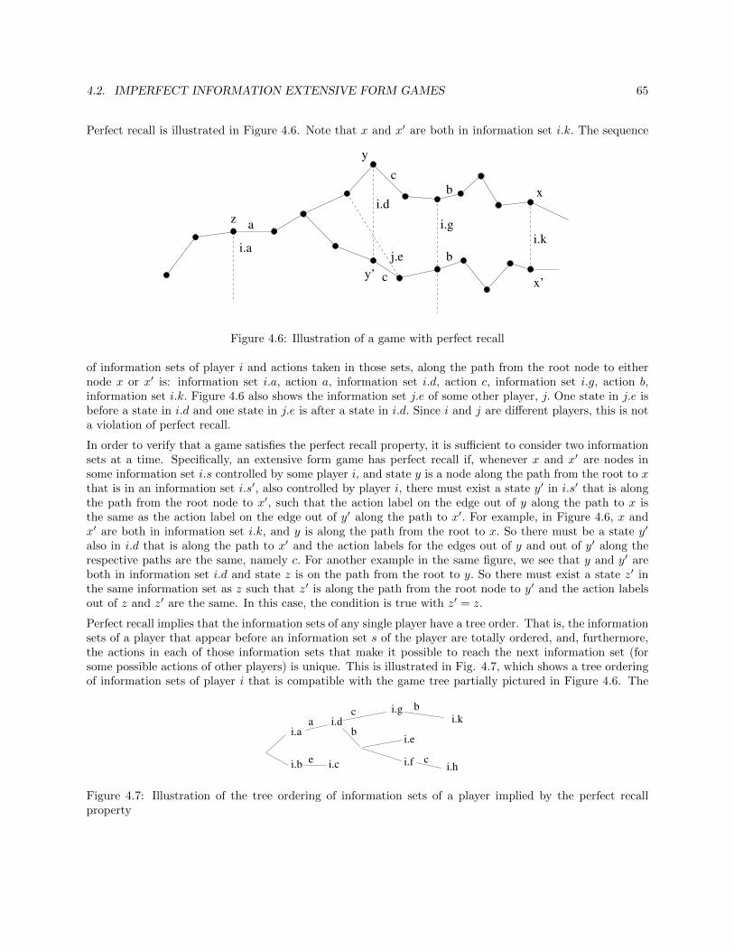
4.2. IMPERFECT INFORMATION EXTENSIVE FORM GAMES 65
Perfect recall is illustrated in Figure 4.6. Note that x and x′ are both in information set i.k. The sequence
z
i.a
i.d
i.g
x
x’
i.k
j.e
a
c
c
b
b
y’
y
Figure 4.6: Illustration of a game with perfect recall
of information sets of player i and actions taken in those sets, along the path from the root node to eithernode x or x′ is: information set i.a, action a, information set i.d, action c, information set i.g, action b,information set i.k. Figure 4.6 also shows the information set j.e of some other player, j. One state in j.e isbefore a state in i.d and one state in j.e is after a state in i.d. Since i and j are different players, this is nota violation of perfect recall.
In order to verify that a game satisfies the perfect recall property, it is sufficient to consider two informationsets at a time. Specifically, an extensive form game has perfect recall if, whenever x and x′ are nodes insome information set i.s controlled by some player i, and state y is a node along the path from the root to xthat is in an information set i.s′, also controlled by player i, there must exist a state y′ in i.s′ that is alongthe path from the root node to x′, such that the action label on the edge out of y along the path to x isthe same as the action label on the edge out of y′ along the path to x′. For example, in Figure 4.6, x andx′ are both in information set i.k, and y is along the path from the root to x. So there must be a state y′
also in i.d that is along the path to x′ and the action labels for the edges out of y and out of y′ along therespective paths are the same, namely c. For another example in the same figure, we see that y and y′ areboth in information set i.d and state z is on the path from the root to y. So there must exist a state z′ inthe same information set as z such that z′ is along the path from the root node to y′ and the action labelsout of z and z′ are the same. In this case, the condition is true with z′ = z.
Perfect recall implies that the information sets of any single player have a tree order. That is, the informationsets of a player that appear before an information set s of the player are totally ordered, and, furthermore,the actions in each of those information sets that make it possible to reach the next information set (forsome possible actions of other players) is unique. This is illustrated in Fig. 4.7, which shows a tree orderingof information sets of player i that is compatible with the game tree partially pictured in Figure 4.6. The
i.h
i.ai.da
ei.b i.c
i.kbi.gc
c
b
i.f
i.e
Figure 4.7: Illustration of the tree ordering of information sets of a player implied by the perfect recallproperty

66 CHAPTER 4. SEQUENTIAL (EXTENSIVE FORM) GAMES
actual path taken through the underlying game tree depends on the actions of the other players and nature.The edge in the tree of Fig. 4.7 from information set i.a to information set i.d means that from at least onestate in i.a, if player 1 plays action a, then it is possible (if actions of other players permit and randomizationprobabilities are not zero) that the game could reach a state in i.d. The tree shown in Fig. 4.7 has a branchpoint after information set i.d. This indicates the possibility for getting from some state in i.d along an edgewith action label b to some state in i.e, or to some state in i.f.
The normal representation of an extensive form game is obtained by having each player select a table ofcontingencies–one for each information set under control of the player. For example, for the game corre-sponding to Fig. 4.7, a pure strategy for player i could look like:
Information set actioni.a ai.b ei.c ei.d ci.e ci.f ci.g bi.h ei.k b
This representation is longer than necessary for some purposes, because, for example, since player i takesaction c in information state i.d, the game cannot reach any of the information sets i.e, i.f, or i.h, so theactions given for those states won’t be used. A mixed strategy for the normal form representation of thegame for a player i is a probability distribution τi over the pure strategies of player i. A mixed strategyprofile for the game in the normal form representation is a tuple τ = (τ1, . . . , τn) of mixed strategies for eachof the players.
Example 4.8 (Normal form of the call my bluff card game) The game tree for the extensive form versionof the call my bluff card game is shown in Fig. 4.4. Player 1 has two information sets. In state 1.a, which isalso an information set of cardinality one, which is entered if the card drawn is red, player 1 decides whetherto take action R (Raise) or action C (Check). In state 1.b, which is entered if the card drawn is black, player1 decides whether to take action r (raise) or action c (check). Thus, there are four pure strategies for player1 in the normal form of the game. Player 2 has one information set that might be reached, namely 2.c, andfor the normal form version of the game player 2 must decide what action to take for that information set:either M (Meet) or P (Pass). So the normal form representation of the call my bluff game is given by thefollowing matrix:
Player 1
Player 2M P
Rr 0,0 1,-1Rc .5,-.5 0,0Cr -.5,.5 1,-1Cc 0,0 0,0
A mixed strategy for player i is equivalent to a joint probability distribution over the sequence of possibleactions for all information sets of player i. Assuming the game has perfect recall, as we do now, allowing

4.2. IMPERFECT INFORMATION EXTENSIVE FORM GAMES 67
arbitrary joint distributions of actions at all information sets is encoding a lot of useless information. Forexample, referring again to either Fig. 4.6 or 4.7, given that player i has to select an action for informationset i.k, the player knows that it previously selected actions a, c, and b for information sets i.a, i.d, and i.g,respectively. And it didn’t have to select any other actions. It doesn’t matter which state of information seti.k the game is in, and the three previous choices by the player were for three information sets, not threeunderlying states. So given the joint distribution of all actions of the player, we can calculate the conditionalprobability distribution σi,i.k of the action player i selects for information set i.k, given that the playerselected actions a, c, and b for information sets i.a, i.d, and i.g, respectively. Such conditional distributionis undefined if the probability of selecting a, c, and b for information sets i.a, i.d, and i.g is zero, in whichcase we let σi,i.k be an arbitrary probability distribution over the actions available for information set i.k.No matter what strategies the other players use, given that player i has to select an action at state i.k, thedistribution of that action is the same under the policy τi and under σi,i.k. We can similarly define σi,s for anyinformation set for player i. Then the tuple of probability distributions for all the information sets of i, σigiven by σi = (σi,s : s is an information set of i), is called a behavioral strategy. And if player i participatesin the game by selecting actions independently for visited information sets using σi, the distribution ofactions made is identical to the distribution of actions made under policy τi. We say the policies σi and τiare behaviorally equivalent.
Any mixed strategy τj of any player j has an equivalent behavioral policy σj , and the strategy profile σgiven by σ = (σ1, . . . , σn) is behaviorally equivalent for the joint interactions of all the players. In particular,the mean payoffs of all players are the same under τ and σ. We state this result as a theorem.
Theorem 4.9 (Kuhn’s equivalence theorem) For an extensive form game with perfect recall for all players,given a strategy profile τ in mixed strategies for the normal form representation of the game, if one or moreof the strategies τi is replaced by the behavioral strategies σi, the probability distribution of which leaf nodein the tree is reached is the same. In particular, the expected payoffs of all players are the same. That is,payoff equivalence holds.
It is considerably simpler to describe a probability distribution over actions for each information set thanto describe a joint probability over all actions a player would use at all information sets. In view of Kuhn’sequivalence theorem, for extensive form games with perfect recall, Nash equilibria represented as profiles ofmixed strategies for the normal form game are equivalent to Nash equilibria for profiles of behavioral strate-gies. In particular, since finite normal form games always have a Nash equilibrium in mixed strategies, weconclude that every extensive form game with perfect recall has a Nash equilibrium in behavioral strategies.We state this as a corollary of Kuhn’s equivalence theorem:
Corollary 4.10 The Nash equilibria of an extensive game with perfect recall in behavioral strategies areprofiles consisting of the the behavioral equivalent strategies of the mixed NE of the normal form version ofthe game.
Multiagent representation of extensive form game Given an extensive form game, the multiagentrepresentation of the game is obtained by replacing each player by a set of players, called agents. There is oneagent for each information set of the player. The underlying game tree is kept the same. An information seti.s controlled by player i in the original game becomes the sole information set controlled by the correspondingagent of player i. The payoff vectors at the leaves of the tree for the multiagent representation of the gamegive the payoffs of each agent, instead of the payoffs of each player, such that the payoff of any agent ofplayer i is the same as the original payoff of the player to which the agent belongs.

68 CHAPTER 4. SEQUENTIAL (EXTENSIVE FORM) GAMES
A behavioral strategy profile σ = (σi)i∈I for an extensive form game is a selection of behavioral strategies ofthe players, and the behavioral strategy of each player is a selection of strategies (i.e. probability distributionsover available actions) for each of the information sets of the player. Thus, σ has one strategy for eachinformation set in the game. Therefore, σ can be viewed as a strategy profile for the multiagent representationof the game, which itself is a game played by the agents.
Proposition 4.11 (Nash equilibrium implies multiagent Nash equilibrium) Consider an extensive form gamewith imperfect information. A Nash equilibrium in behavioral strategies for an extensive form game is alsoa Nash equilibrium for the multiagent representation of the game.
The converse of Proposition 4.11 fails, as shown by the following example.
Example 4.12 (Mutliagent Nash equilibrium does not imply Nash equilibrium for original players) Considerthe single player extensive form game of Fig. 4.8. There is a unique Nash equilibrium strategy for player 1
Down
1.a
1.b
1
0
2up
down
Up
Figure 4.8: Example of a multiagent Nash equilibrium, namely (Down, down), that is not a Nash equilibriumfor the original single player game.
in the normal form representation of the game, namely, (Up, up). For the multiagent representation of thegame, one agent controls the decision at node 1.a and another agent controls the decision at node 1.b, andthe numbers at the leaves give the payoffs of both agents. The strategy pair (Up, up) is indeed a multiagentNash equilibrium, as guaranteed by Proposition 4.11. However, (Down, down) is also a multiagent Nashequilibrium. Indeed, if the first agent were to change action to Up then the payoff of the first agent woulddecrease from 1 to 0. If the second agent were to change from down to up, the payoff of the second agentwould still be 1. The point of the example is that a single player can change its strategy from (Down, down)to (Up, up) to increase his/her payoff, but no one agent alone could do the same. Of course this examplecould be extended to make examples involving multiple players.
Example 4.12 suggests that the multiagent representation of the game is not so interesting. However, themulitagent representation is very useful for a more restrictive definition of equilibrium, as seen in the nextsection.
4.2.2 Sequential equilibria – generalizing subgame perfection to games withimperfect information
For perfect information games we saw that there is some reason to think that subgame perfect Nash equi-libria are more preferable or realistic than other Nash equilibria. In particular, as illustrated in the entrydeterrence game, restricting attention to subgame perfect equilibria eliminates some threats that are notcredible. The notion of sequential rationality, discussed in this section, is a way to extend the notion ofsubgame perfect equilibrium to extensive form games with imperfect information.

4.2. IMPERFECT INFORMATION EXTENSIVE FORM GAMES 69
Example 4.13 Consider the minor variation of the entry deterrence game of Example 4.1 shown in Fig.4.9. The edge corresponding to the action “in” in the original game tree is replaced by two edges with
2,1
1.a
1,2
out
2.a
accommodate
fight
accommodate
fight
0,0
0,0
in1
2in
2,1
Figure 4.9: The entry deterrence game modified by the addition of a random coin toss
corresponding actions “in1” and “in2,” that are equivalent to “in” in the original. Nevertheless, there arenow no subgames beginning at a state (i.e. node) of the graph, other than the root node. We thus consider(out, fight) to be a subgame perfect equilibrium. That is, the concept of subgame perfect based on gamesstarting at individual states of the game don’t rule out the not credible threat represented by player 2 using“fight.”
Information sets are used to model imperfect information in extensive form games. A player must select anaction for an information set without knowing which state in the set the game is in. In order to judge whethera player is rationally controlling an information set, it would help to know the probability distribution overthe states of the information set the player is assuming. The player might say, “Of course I made a rationaldecision. Given information set s, I calculated that state x had conditional probability 0.9 and state y hadconditional probability 0.1, so I weighted the potential expected payoffs accordingly to select an action forthat information set.” In order for this statement to be credible, it should be checked that the strategyemployed by the player is indeed rational for the stated beliefs, and checked that the stated beliefs areconsistent with the game structure and the strategies used by the players and nature. These notions areformalized in what follows.
A belief vector µ(s) for an information set s consists of a probability distribution (µ(x|s) : x ∈ s) over thestates in the information set. A belief vector µ for the entire game is a vector µ = (µ(s)) for every informationset in the game. A pair (σ, µ) consisting of a behavioral strategy profile σ and a belief vector µ is called anassessment.
For an extensive form game with imperfect information, payoffs are determined by which leaf node is reachedin the game tree. Let ui(σ|x) denote the expected payoff of player i under strategy profile σ beginningfrom state x. Note that ui(σ|x) depends only on the decisions made at x and later in the game. For aninformation set s and belief vector µ(s), let ui(σ|s, µ(s)) =
∑x∈s ui(σ|x)µ(x|s). Also, for a state of the game
x and behavioral strategy profile σ, let p(x|σ) denote the probability that the game visits state x. Given thebehavioral strategy profile σ and an information state s, it is natural to let µ(s) = (µ(x|s) : x ∈ s) be theconditional probability distribution of the state, given that the state is in information set s:
µ(x|s) =p(x|σ)∑
x′∈s p(x′|σ)
(4.1)
The righthand side of (4.1) is well defined if the denominator is greater than zero. In that case, we couldconsider the pair (s, µ(s)) to be a generalized state of the game. However, the righthand side of (4.1) is notwell defined if the denominator is zero, i.e., if the probability of reaching information set s is zero. If wethink of large games with perfect information, there might be large numbers of states that have probabilityzero under a strategy profile, and yet we would like the actions taken by players in those states to be rational

70 CHAPTER 4. SEQUENTIAL (EXTENSIVE FORM) GAMES
in case some changes were made and those states were reached. So by analogy, in games with imperfectinformation, we would like players to make rational decisions at information sets even if the informationsets are off the game path with probability one for the strategy profile under consideration. It would be tooarbitrary to allow for arbitrary probability distributions over the set of states in an information set in suchcases.
The idea of Kreps and Wilson [9] is to consider distributions that could arise by small perturbations ofthe policies. A player’s strategy in a normal form game is completely mixed if it assigns (strictly) positiveprobability to each of the player’s possible actions. Let Σo be the set of completely mixed behavioralstrategy profiles and let Σo denote the set of assessments such that σ ∈ Σo and µ is computed from σ foreach information set using (4.1):
Ψo =
(σ, µ) : σ ∈ Σo, µ(x|s) =
p(x|σ)∑x′∈s p(x
′|s)
.
Definition 4.14 (Sequential equilibrium) For an extensive form game with perfect recall:
(SR) An assessment (σ, µ) is sequentially rational if for any information set s and any alternative probabilitydistribution σ′s over the actions at s available to the player i that controls s,
ui(σ′s, σ−s|s, µ(s)) ≤ ui(σ|s, µ(s)),
where σ−s is the set of mixed strategies used by all players at all information sets, except for player iat information set s.
(C) An assessment (σ, µ) is consistent if there exists (σk, µk) ∈ Ψo for k ≥ 1 such that (σ, µ) = limk→∞(σk, µk).
A sequential equilibrium is an assessment (σ, µ) that is (SR) sequentially rational and (C) consistent.
Remark 4.15 (a) Sequential equilibrium, defined in Definition 4.14, requires (SR) sequential rationality,which involves perturbations of the behavioral strategy of a given player only for one information set ata time. Thus below we will see further use of the multiagent representation of the game.
(b) Consider a behavioral strategy profile σ. If an information set s is such that∑x′∈s p(x
′|s) > 0, then µ(s)for any consistent assessment (σ, µ) must satisfy (4.1) because the righthand side of (4.1) is continuousin a neighborhood of σ. Furthermore, if σ is a Nash equilibrium then the behavioral strategy σs used forthe information state s must be rational for the player using it. In particular, if σ is a fully mixed strategyprofile and is a Nash equilibrium, and if µ is defined by (4.1), then (σ, µ) is a sequential equilibrium.Conversely, if (σ, µ) is a sequential equilibrium, σ is a Nash equilibrium.
(c) (Sequential equilibrium generalizes the notion of subgame perfect) A sequential game with perfect infor-mation is a special case of a sequential game with imperfect information, such that each informationset contains only a single node. For a perfect information game there is only possible belief vector µ,namely, for each information set s, assigning probability one to the unique node x in s. Moreover, anassessment (σ, µ) is consistent for any behavioral strategy profile σ, and it is a sequential equilibrium ifand only if σ is subgame perfect.
Definition 4.16 A trembling hand perfect (THP) equilibrium of a finite normal form game is a strategyprofile σ = (σi) such that there exists a sequence of completely mixed strategy profiles (σk) converging to σsuch that for each k and each player i, σi is a best response to σk−i for all k.

4.2. IMPERFECT INFORMATION EXTENSIVE FORM GAMES 71
Remark 4.17 (a) A trembling hand perfect equilibrium is a Nash equilibrium.
(b) A trembling hand perfect equilibrium of the normal representation of an extensive form game with perfectinformation is not necessarily subgame perfect (See Example 250.1 of Osborne.) Instead, we considertrembling hand perfect equilibria of the multiagent representation of the game.
Proposition 4.18 Consider an extensive form game with perfect recall. If σ is a trembling hand perfectequilibrium of the multiagent representation of the game, then there exists a belief system µ such that (σ, µ)is a sequential equilibrium.
Proof. Suppose σ is a trembling hand perfect equilibrium of the multiagent representation of the game,so there exits a sequence σk, k ≥ 1, of fully mixed behavioral strategy profiles such that σk → σ and, foreach information set s, σs is the best response to σk−s for the agent controlling state s. Let µk denote thebelief vector obtained by applying (4.1) with σ replaced by σk, so (σk, µk) ∈ Ψo for all k ≥ 1. Since theset of all belief vectors is a compact set, there is a subsequence kj → ∞ as j → ∞ such that µkj → µ forsome belief vector µ. To avoid messy notation, assume without loss of generality that the entire sequenceµk is convergent with limit µ, that is, µk → µ as k → ∞. We claim (σ, µ) is a sequential equilibrium. Byconstruction, (σk, µk) → (σ, µ), so the assessment (σ, µ) is consistent (C). It remains to show that (σ, µ) issequentially rational (SR).
By assumption, for any information set s, σs is the best response to σk−s, which means that for any alternativemixed strategy σ′s available to the player i controlling information set s,∑
x∈Sui(σ
′s, σ
k−s|x)µk(x|s) ≤
∑x∈S
ui(σs, σk−s|x)µk(x|s) (4.2)
As k →∞, ui(σ′s, σk−s|x)→ ui(σ′s, σ−s|x) and µk(x|s)→ µ(x|s). Thus, taking the limit k →∞ on each side
of (4.2) yields ∑x∈S
ui(σ′s, σ−s|x)µ(x|s) ≤
∑x∈S
ui(σs, σ−s|x)µ(x|s),
or more concisely, ui(σ′s, σ−s|x, µ(s)) ≤ ui(σs, σ−s|x, µ(s)). Therefore, the assessment (σ, µ) is (SR) sequen-
tially rational.
Proposition 4.19 (Existence of trembling hand perfect equilibrium (Selton 1975)) A finite normal formgame (I, (Ai : i ∈ I), (ui)i∈I) has at least one trembling hand perfect equilibrium.
Proof. Let ε be so small that ε < 1/L, where L is the maximum over all players of the number of actionsavailable to player i. Let T ε denote the set of mixed strategy profiles for the game such that each playerplays each action with probability at least ε. By the existence theorem for Nash equilibria for convex games,there exists a Nash equilibrium τ ε for the game with strategy profiles T ε, for any ε > 0.
Since the set of mixed strategy profiles is compact, there is a sequence εk → 0 as k → ∞ such that (τ εk)converges. Let τ = limk→∞ τ εk . For any player i and action ai such that τi(ai) > 0 it follows that τ εki (ai) > 0for all k sufficiently large. Since there is a finite set of players, each with a finite set of actions, there is aK large enough that τ εki (ai) > 0 for all k ≥ K for any player i and action ai such that τi(ai) > 0. Thecondition τ εki (ai) > 0 implies that ai is a best response action to τ εk−i. So if k ≥ K, any action for any playeri that has positive probability under τ is a best response action for player i against τ εk−i. Thus, (τ εK+k)k≥0

72 CHAPTER 4. SEQUENTIAL (EXTENSIVE FORM) GAMES
is a sequence of completely mixed strategy profiles such that τi is a best response to τεK+k
−i for all i ∈ I andall k ≥ 0. Thus, τ is a trembling hand perfect equilibrium of the game.
The following is an immediate consequence of Propositions 4.18 and 4.19.
Corollary 4.20 Every finite extensive form game with perfect recall has at least one sequential equilibrium(σ, µ).
The following may be of some help in identifying trembling hand equilibria.
Definition 4.21 (Weakly dominated strategy in normal form game) An action a of a player i in a normalform game is weakly dominated if there is a mixed strategy α such that ui(α, s−i) ≥ ui(a, s−i) for all s−iand ui(α, s−i) > ui(a, s−i) for at least one specific choice of s−i.
Proposition 4.22 (i) In a trembling hand perfect equilibrium, the strategy of any player assigns zero proba-bility to any weakly dominated action. (ii) The converse is true for two player games: For two player games,a Nash equilibrium such that the strategy of neither player is weakly dominated is a trembling hand perfectequilibrium. (See [15, Prop. 248.2]).
Example 4.23 (Revisiting the entry deterrence game) The entry deterrence game, described in Example4.1, is the perfect information extensive form game with the game tree shown in Figure 4.10. It is easy to
in
1.a
accommodate
fight
0,0
1,2
2,12.a
out
Figure 4.10: Game tree for the entry deterrence game
verify that (in, accommodate) is the unique subgame perfect equilibrium by using Proposition 4.3. But it isinstructive to see how Propositions 4.22 and 4.18 can be used to deduce that (in, accommodate) is subgameperfect based on the normal form of the game.
The normal form of the game is given in Table 4.1. This game has two Nash equilibria in pure strategies:
Table 4.1: Normal form of entry deterrence game
Player 1
Player 2accommodate fight
in 2,1 0,0out 1,2 1,2
(out, fight) and (in, accommodate), as well as some Nash equilibria in mixed strategies. Just looking atthe normal form of the game, we see that accommodate weakly dominates any other strategy for player 2.Thus, by Proposition 4.22, any Nash equilibrium that is THP must have player 2 using accommodate, whichimplies that (in, accommodate) is (the unique) trembling hand perfect equilibrium for the normal form of thegame. Since each player only controls one information set, the original form of the game is equivalent to

4.3. GAMES WITH INCOMPLETE INFORMATION 73
the multiagent form (for either the sequential or normal representation). Thus, Proposition 4.18 (also seeRemark 4.15(c)) implies that (in, accommodate) is a subgame perfect equilibrium.
4.3 Games with incomplete information
Often when players participate in a game, they lack potentially relevant information about the motivationsof the other players. Games of incomplete information (also called Bayesian games) are defined to modelthis situation in a Bayesian framework.
Definition 4.24 A (finite) game of incomplete information is given by G = (I, (Si)i∈I , (Θi)i∈I , (ui(s, θ))i∈I , p(θ))such that
• I is the set of players, assumed to be finite
• Si is a finite set of actions available to player i for each i ∈ I, and S = Xi∈ISi is the set of actionprofiles, with a typical element s = (si)i∈I .
• Θi is a finite set of possible types of player i and Θ = Xi∈IΘi is the set of type assignments for allplayers, with a typical element θ = (θi)i∈I .
• ui(s, θ) is the payoff of player i for given s and θ.
• p is a probability mass function (pmf) over Θ (i.e. a joint probability mass function for types). Themarginal pmfs, given by p(θi) =
∑θ−i
p(θi, θ−i), are assumed to be strictly positive, so the conditional
pmfs, p(θ−i|θi), are well defined.
The operational meaning is that at the beginning of the game, nature selects a type assignment θ using pmfp, and each player i learns its own type, θi. Players are not told the types of the other players; θi is consideredto be the private information of player i. However, all players are assumed to know p, so each player i knowsp(θ−i|θi), the conditional probability distribution of the types of the other players. After learning their types,the players each select an action the can depend on their respective types; a pure strategy si for a player iis a mapping si : Θi → Si.
A profile of pure strategies (si(·))i∈I is a Bayesian (or Bayes-Nash) equilibrium for the game if for each i ∈ Iand each θi ∈ Θi,
si(θi) ∈ arg maxa′i∈Si
∑θ−i
p(θ−i|θi)ui(a′i, s−i(θ−i), θi, θ−i). (4.3)
The sum on the righthand side of (4.3) is the expected payoff of player i given the type of the player, θi,given player i takes action a′i. A mixed strategy for player i is a randomized pure strategy. A profile ofmixed strategies is a Bayesian (or Bayes-Nash) equilbribum if for each i, the expected payoff of player i ismaximized by its randomized strategy, given the randomized strategies used by the other players.
A finite Bayesian game is a special case of an extensive form game with imperfect information. Indeed, givena finite Bayesian game, construct the game with imperfect information as follows. The root node of thegame tree would be controlled by nature, which selects θ = (θ1, . . . , θn), where we assume I = [n]. There isone edge of the tree directed out of the root node for each possible assignment of types θ. Then there aren stages of the game tree following the root node, where n is the number of players. The nodes in the firststage are all controlled by player 1. The fact player 1 should know θ1 can be indicated by partitioning the

74 CHAPTER 4. SEQUENTIAL (EXTENSIVE FORM) GAMES
nodes in stage one into information states controlled by player 1, one for each possible value of θ1. Eachnode in stage one has an outgoing edge for each possible action of player 1. In general, the nodes in stage iare partitioned into information sets controlled by player i, one for each possible value of θi. When player imakes a decision he/she does not know the types of the other players or the actions taken earlier in the treeby other players.
In turn, there is a normal form version of a Bayesian game. Each player i has a finite set of possible choices offunctions si : Θi → Si, and if all players make such a choice the expected payoff of each player is determinedby the game. For any finite Bayesian game, a Bayesian equilibrium in mixed strategies exists. This is aconsequence of the existence of Nash equilibrium for imperfect information games, or for finite normal formgames, which follow from the Kakutani fixed point theorem.
The call my bluff game of Example 4.5 can be viewed as a game of incomplete information by thinking ofthe color of the card as the type of player 1. Player 2 always has one possible type. An example of analternative interpretation of the game is the following. We could imagine the players as entering a possiblebattle, with the strength of the first player being random and known only to the first player. The red typefor player 1 means player 1 is strong, and black type means player 1 is weak. The action raise for player 1means player 1 boasts about his/her strength in some way by some provocative action. If player 1 raises,player 2 can decide to either stay in (meet), or surrender (pass).
Example 4.25 (A Cournot game with incomplete information) Given c > a > 0 and 0 < p < 1, considerthe following version of a Cournot game. Suppose the type θ1 of player 1 is either zero, in which case hisproduction cost is zero, or one, in which case his production cost is c (per unit produced). Player 2 has onlyone possible type, and has production cost is c. Player 1 knows his type θ1. It is common knowledge thatplayer 2 believes player 1 is type one with probability p. Both players sell what they produce at price per unita − q1 − q2, where qi is the amount produced by player i. A strategy for player 1 has the form (q1,0, q1,1),where q1,θ1 is the amount produced by player one if player 1 is type θ1. A strategy for player 2 is q2, theamount produced by player 2.
The best response functions of the players are given by:
q1,0 = arg maxq1
q1(a− q2 − q1) =(a− q2)+
2
q1,1 = arg maxq1
q1(a− c− q2 − q1) =(a− c− q2)+
2
q2 = arg maxq′2
(1− p)q′2(a− c− q1,0 − q′2) + pq′2(a− c− q1,1 − q2)
= arg maxq′2
q′2(a− c− q1 − q′2) =(a− c− q1)+
2
where q1 = (1− p)q1,0 + pq1,1.
Next, we dentify the Bayes-Nash equilibrium of the game, assuming for simplicity that a ≥ 2c. Substitutingthe best response functions for player one into the definition of q1, yields
q1 =a− pc− q2
2
so that we have coupled fixed point equations for q1 and q2. Seeking strictly positive solutions we have
q2 =(a− c− q1)+
2=
(a− c− a−pc−q22 )
2=a− (2− p)c+ q2
4

4.3. GAMES WITH INCOMPLETE INFORMATION 75
which can be solved to get
q2 =a− (2− p)c
3, q1.0 =
2a+ (2− p)c6
, q1,1 =2a− (1 + p)c
6,
Furthermore, q1 = a+(1−2p)c3 .
After finding the equilibrium, it can be shown that the three corresponding payoffs are given by
u2(qNE) =(a− (2− p)c)2
9
and
u1(qNE |θ1 = 0) =(2a+ (2− p)c)2
36, u1(qNE |θ1 = 1) =
(2a− (1 + p)c)2
36.
As expected, u2(qNE) is increasing in p, and both u1(qNE |θ1 = 0) and u1(qNE |θ1 = 1) are decreasing inp with u2(qNE) < u1(qNE |θ1 = 1) < u1(qNE |θ1 = 0) for 0 < p < 1. In the limit p = 1, u2(qNE) =
u1(qNE |θ1 = 1) = (a−c)29 , as in the original Cournot game with complete information and production cost c
for both players.

76 CHAPTER 4. SEQUENTIAL (EXTENSIVE FORM) GAMES

Chapter 5
Multistage games with observedactions
5.1 Extending backward induction algorithm – one stage devia-tion condition
A multistage game with observed actions is such that:
• The game progresses through a sequence of stages, possibly infinitely many. Often each stage is also atime period.
• Players select actions simultaneously within a stage.
• Players know the actions of all players in previous stages.
For a finite number of stages these games can be modeled as extensive form games with imperfect information(imperfect because of the simultaneous play within each stage). The following notation will be used. Forsimplicity, it is assumed that the players use pure strategies, but the propositions hold also for the case ofmixed strategies – see Remark 5.8 below.
• ai(t) is the action of player i at stage t for 1 ≤ i ≤ n and t ≥ 1, with ai(t) ∈ Ai, where Ai is a finiteset of possible actions for player i at any stage.
• ht = (ai(r) : 1 ≤ i ≤ n, 1 ≤ r ≤ t − 1) is the history at stage t, recording the actions taken strictlybefore stage t.
• Ht is the set of all tuples of the form (ai(r) : 1 ≤ i ≤ n, 1 ≤ r ≤ t− 1) such that ai(r) ∈ Ai for all i, r.The set Ht thus includes all possible histories, assuming no restrictions on what actions players cantake at each stage.
• A (pure strategy) policy for player i, si, maps (stage, history) pairs to action: si(t, ·) : Ht → Ai Theaction si(t, ht) should be defined for all ht ∈ Ht, even if ht is not consistent with the values of policysi for earlier stages. If policy si is used and ht is the history at stage t, then the action selected byplayer i is ai(t) = si(t, ht).
77

78 CHAPTER 5. MULTISTAGE GAMES WITH OBSERVED ACTIONS
• Payoff functions: Ji(si, s−i) =∑Kt=1 ui(t, si(t, ht), s−i(t, ht)), where ui is the stage payoff function for
player i. The horizon K is possibly +∞.
For a given k fixed with 1 ≤ k ≤ K and history hk, the subgame for (k, hk) is the game with payoff
functions J(k)i (si, s−i|hk) =
∑Kt=k ui(t, si(t, ht), s−i(t, ht)). It only depends on sj ’s for t ≥ k. A strategy
profile (sj : 1 ≤ j ≤ n) is a subgame perfect equilibrium if it is a Nash equilibrium for every subgame (k, hk).
Example 5.1 (Trigger strategy for six-stage prisoners’ dilemma game) Consider a six-stage game, such thateach stage consists of one play of the prisoners’ dilemma game. The payoff of player i for the six stage gameis the sum of the players payoffs from the six stages. The payoffs for the prisoners’ dilemma game are giveby the following table:
Player 1
Player 2C (cooperate) D
C (cooperate) 1,1 -1,2D 2,-1 0,0
Strategy D is a dominant strategy for each player for the single shot game.
Consider the following trigger strategy sT for player i (the superscript “T” is for “trigger”): Play C in eachstage if no player has ever played D earlier. Otherwise, play D. Intuitively, each player is initially beinggenerous, with the idea being that the other player will have incentive to cooperate at each stage because itwill improve the options for the other player in future stages. If both players use the trigger strategy, they willboth play C in all six stages, so they both receive payoff 6. Sounds good. But is (sT , sT ) a Nash equilibrium?
No matter what happens in the first five stages, for any Nash equilibrium, the best response action for aplayer in the final stage of the game is to play D. So for any Nash equilibrium, both players play D in stage6 and both get zero reward in stage 6. Therefore, no matter what happens in the first four stages, for anyNash equilibrium, the best response action for a player in the fifth stage of the game is to play D. So forany Nash equilibrium, both players play D in stage 5 and both get zero reward in stage 5. Continuing withthis reasoning for stages 4 down to stage 1, we find that the behavior of the players is unique for and Nashequilibrium for the six stage game, namely, both players play D in every stage, and the payoff vector is (0, 0).In particular, (sT , sT ) is not a Nash equilibrium. More generally, the behavior of both players is to alwaysplay D for any subgame perfect equilibrium.
Consider the following variation of the example. After each stage, one of the players rolls a fair die to generatea random integer uniformly distributed from 1 to 6, observed by all players. If the number 6 appears, theplayers stop and the game is over. Else, the players continue to another stage. The total number of stages
X is thus random, and it has the geometric distribution with parameter p = 16 ; P X = k = 1
6
(56
)k−1for
k ≥ 1 and E [X] = 6. Both players always playing D is again a subgame perfect equilibrium. Are there anyother subgame perfect equilibria? How about if both players play the trigger strategy defined above?
We claim the trigger strategy profile (sT , sT ) is subgame perfect. To prove it, consider an arbitrary subgame(k, hk). We need to show (sT , sT ) is a Nash equilibrium for the subgame. The subgame (k, hk) is reachedonly if X ≥ k, so the expected subgame payoffs are computed conditioned on X ≥ k.Consider two cases. In the first case, the history hk indicates at least one of the players selected D at somestage before k, and hence under (sT , sT ) each player will play D in every stage from stage k until the end.Even if one of the players, i, were to use a different strategy for the subgame, the other player would still playD in every stage of the subgame. Thus, player i would get a strictly smaller payoff whenever he/she played

5.1. EXTENDING BACKWARD INDUCTION ALGORITHM – ONE STAGE DEVIATION CONDITION79
C instead of D during the subgame. So player i would have no incentive to not use sT for the subgame.
In the second case, the history hk indicates that both players selected C in all stages before stage k. Thus,from stage k forward, both players use a trigger strategy starting at stage k just as they would for the entiregame starting at stage 1. Also, by the memoryless property of the independent die rolls, the number of stagegames that will be played for the subgame (k, hk) has the same distribution as the number of stages thatare played for the original game.
By symmetry we consider only the case that player 2 uses the trigger strategy sT for the subgame andplayer 1 uses some other strategy s′1. Let Y , with Y ≥ k, denote the first stage player 1 would play D understrategy s′1, if the game doesn’t end first. We fix y ≥ k and focus on the difference in payoffs on the eventY = y. By averaging over y, by the law of total probability, we can calculate the expected difference ofpayoffs for Y random. Given Y = y, the payoffs for player 1 are the same for s1 and s′1 up to stage y− 1. Inparticular, if X ≤ y − 1, the game ends before the policies diverge, and the difference in payoffs is zero. Sowe can restrict attention to conditioning on the event Y = y,X ≥ y and consider the expected differencein payoffs for stage y until the end of the game. Given X ≥ y, the conditional distribution of the number ofstages remaining starting with state y has the same geometric distribution, with mean 6, as the number ofstages in the original game. Thus, the expected payoff of player 1 from stage y onward, given player 1 usesstrategy sT , is 6. If instead player 1 uses s′1 and thus plays D for the first time at stage y, the payoff is 2.Since 2 < 6, player 1 has a smaller expected payoff under s′1.
Thus, (sT , sT ) is subgame perfect as claimed. This reasoning would be true if the probability of continuingat each stage, instead of being 5/6, were anything greater than or equal to 1/2.
Definition 5.2 A strategy profile s∗ satisfies the one-stage-deviation (OSD) condition if for any i, k, hk with1 ≤ k ≤ K, if s agrees with s∗ except at i, k, hk, then
J(k)i (si, s
∗−i|hk) ≤ J (k)
i (s∗i , s∗−i|hk). (5.1)
Remark 5.3 If K is finite and deterministic, then s∗ satisfies the one stage deviation condition if and onlyif it can be derived using backwards induction.
Proposition 5.4 (One-stage-deviation principle for multistage games with observed actions, K finite) Astrategy profile s∗ is a subgame perfect equilibrium (SPE) if and only if s∗ satisfies the one-stage-deviationcondition.
Proof. (only if) If s∗ is an SPE, then by definition, for any i, k, hk with 1 ≤ k ≤ K, (5.1) is true for anystrategy si for player i, including one that differs from s∗i only at stage k for history hk. Thus, s∗ satisfiesthe OSD condition.
(if) Suppose s∗ satisfies the OSD. Let i be an arbitrary player and let si be an arbitrary strategy for i. Toshow that s∗ is an SPE, it suffices to show that for 1 ≤ k ≤ K,
J(k)i (si, s
∗−i|hk) ≤ J (k)
i (s∗i , s∗−i|hk), for all hk. (5.2)
We use proof by backwards induction on k. For the base case, note that (5.2) is true for k = K, because foreach choice of hK , the only way si enters either side of (5.2) is through its value for stage K and historyhK , si(K,hK). Thus, for this case, (5.2) is an instance of the OSD condition, assumed to hold.
For the general induction step, suppose (5.2) is true for k + 1, for some k with 1 ≤ k ≤ K − 1. Consider anarbitrary choice of hk, and let hk+1 be an extension of hk using si(k, hk) and s∗−i(k, hk):
hk+1 = (hk, si(k, hk), s∗−i(k, hk)).

80 CHAPTER 5. MULTISTAGE GAMES WITH OBSERVED ACTIONS
Then
J(k)i (si, s
∗−i|hk) = ui(k, si(k, hk), s∗−i(k, hk)) + J
(k+1)i (si, s
∗−i|hk+1)
(a)
≤ ui(k, si(k, hk), s∗−i(k, hk)) + Jk+1)i (s∗i , s
∗−i|hk+1)
(b)= J
(k)i (si, s
∗−i|hk)
(c)
≤ J(k)i (s∗i , s
∗−i|hk),
where (a) holds by the induction hypothesis, (b) holds for si defined to agree with si at (k, hk) and with s∗ielsewhere, and (c) holds by the OSD condition.
The one step deviation principle can be extended to K = +∞ under the following condition:
Definition 5.5 The game is continuous at infinity if
limk→∞
supi,s,s,hk
∣∣∣∣J (k)i (s|hk)− J (k)
i (s|hk)
∣∣∣∣ = 0.
The game is continuous, for example, if the stage game payoffs have the form gi(s(t), ht)δt−1 for a bounded
function gi and a discount factor δ with 0 < δ < 1.
Proposition 5.6 (One-stage deviation principle for infinite horizon) Consider the game with infinite hori-zon, K = +∞.. If the game is continuous at infinity then s∗ is a subgame perfect equilibrium (SPE) if andonly if the one step deviation (OSD) condition holds.
Proof. (only if) This part of the proof is the same as for Proposition 5.4 for K finite.
(if) Suppose s∗ satisfies the OSD condition. Let ε > 0. Fix i and a policy si for player i. If suffices to show:
J(k)i (si, s
∗−i|hk) ≤ J (k)
i (s∗i , s∗−i|hk) + ε for all hk (5.3)
for all k. By the continuity at infinity condition, there exists k so large that (5.3) is true for all k < k. The
backwards induction proof used to prove Proposition 5.4 for K finite can be used to show (5.3) for 0 ≤ k ≤ kas well, and hence for all k.
Example 5.7 To demonstrate the use of the OSD principle, let’s revisit the variation of the trigger strategyfor repeated prisoner’s dilemma game with random stopping as discussed above. Instead of stopping thegame with probability δ after each stage, suppose the game continues for infinitely many stages, but weightthe payoffs for stage t by the probability that the stage is reached: (1− δ)t−1. Also multiply the payoffs by theconstant factor (1− δ) for convenience, arriving at the stage payoffs: ui(t, s(t, ht)) = (1− δ)δt−1gi(st(t, ht)),where gi is the payoff function for one play of prisoners’ dilemma (e.g. g1((C,C)) = 1, g1((C,D)) = −1,etc.). Let sT be the trigger strategy of playing C in every stage until at least one player plays D, and thenswitch to playing D thereafter.
Let us show that (sT , sT ) satisfies the OSD condition if 0.5 ≤ δ < 1, implying (sT , sT ) is a subgame perfectequilibrium if 0.5 ≤ δ < 1. Fix i ∈ 1, 2 (and let −i denote the other player), fix k ≥ 1 and a history hk.(For example, i = 1, k = 4 and h4 = ((C,C), (C,D), (D,C)).) Consider two cases.

5.2. FEASIBILITY THEOREMS FOR REPEATED GAMES 81
Case 1: D appears at least once within hk. Both players play D at state (k, hk) under (sT , sT ). So there isonly one choice for si in the definition of the OSD condition, namely, play C at state (k, hk) and follow sT
otherwise. Both players will play D at all stages after stage k under both si and sT for player i. Thus,
J(k)i (s∗i , s
∗−i|hk)− J (k)
i (si, s∗−i|hk) = (0− (−1))(1− δ)δk−1 > 0.
Case 2: D does not appear within hk. Both players play C at stage (k, hk) under (sT , sT ). So there is only onechoice for si in the definition of the OSD condition, namely, play D at state (k, hk) and follow sT otherwise.With player i using si, both players will play D after stage k. Thus,
J(k)i (s∗i , s
∗−i|hk)− J (k)
i (si, s∗−i|hk) = ((1 + δ + δ2 + · · · )− 2)(1− δ)δk−1 = (1− 2(1− δ))δk−1 ≥ 0,
if 0.5 ≤ δ < 1.
Thus, the OSD condition is satisfied if 0.5 ≤ δ < 1, as claimed.
Remark 5.8 Up to this point, this section considers pure strategies, so that, given i, t, and ht, si(t, ht) isa particular action in Ai. However, Propositions 5.4 and 5.6 readily extend to mixed strategies in behavioralform. Example 4.6 illustrates the fact that single shot (aka normal form) games can be considered to bespecial cases of extensive form games. By the same idea, multistage games with observed actions and a finitenumber of stages can also be viewed as examples of extensive form games. Moreover, they are extensiveform games with perfect recall. Thus, by Kuhn’s equivalence theorem, Theorem 4.9, any mixed strategy τifor a multistage game, which is a mixture of pure strategies of the form si considered above, is behaviorallyequivalent to a behavioral strategy σi. The result holds also if K = ∞ for games that are continuous atinfinity. A behavioral strategy for player i, σi, maps (stage, history) pairs to Ai, where Ai is the set ofprobability distributions over Ai. Thus, σi(t, ht) ∈ A for 1 ≤ t ≤ K and ht ∈ Ht.
The set of histories Ht is the same whether pure strategies or behavioral strategies are used. If player i usesbehavioral strategy σi, then σi(t, ht) is the probability distribution for the action ai(t) selected by player i attime t. The other players observe the action ai(t) but do not observe σi(t, ht).
5.2 Feasibility theorems for repeated games
Let G = (I, (Ai)i∈I , (gi)i∈I) be a finite normal form game and let 0 < δ < 1. The repeated game with stagegame G and discount factor δ is the normal form game with payoff functions
Ji(s) = (1− δ)∞∑t=1
δt−1gi(s(t, ht)),
where s is a profile of pure strategies, s = (si(t, ht))i∈I,t≥1. Since (1− δ)∑∞t=1 δ
t−1 = 1, if each player usesa constant strategy si(t, ht) ≡ ai then Ji(s) = gi(a) for all i.
In this section we consider behavioral strategies (see Remark 5.8). Let Ai be the set of probability dis-tributions on Ai, and write αi for a typical element of Ai and ai for a typical element of Ai. A profile ofmixed strategies for the stage game has the form α = (αi)i∈I . The interpretation of α is that the playersindependently select actions, with player i selecting an action in Ai at random with distribution αi. Fora profile of mixed strategies α and a fixed player i, α−i represents a joint distribution over the actions ofthe other players, such that the actions of the other players are mutually independent. A profile of mixedstrategies in behavioral form for the multistage game is a tuple σ = (σi)i∈I such that, for any k ≥ 1 and

82 CHAPTER 5. MULTISTAGE GAMES WITH OBSERVED ACTIONS
history hk ∈ Hk, σi(k, hk) ∈ Ak. For k and hk fixed, (σi(k, hk))i∈I is a mixed strategy profile for the stagegame. In particular, if (ai(k))i∈I denotes the random actions taken at stage k, the actions are conditionallyindependent given (k, hk). The expected reward for player i in the repeated game is written as
Ji(σ) = (1− δ)∞∑t=1
δt−1gi(σ(t, ht)),
where gi(σ(t, ht)) is the expected reward for player i in the stage game for the profile of mixed strategiesσ(t, ht) = (σi(t, ht))i∈I . That is,
gi(σ(t, ht)) =∑
a∈×i∈I Aigi(a)
∏i∈I
σi(ai|t, ht).
Just as for pure strategy profiles, if α is a mixed strategy profile for the stage game, and if σ is the behavioralstrategy profile for the repeated game with σi ≡ αi, then J(σ) = g(α).
We have seen that there can be multiple equilibria for the repeated game even if the stage game has a uniqueNash equilibrium. For example, it is true if the stage game is prisoners’ dilemma. Feasibility theoremsaddress what payoff vectors can be realized in equilibrium for repeated games for δ sufficiently close to one.
Let v = (vi)i∈I be the vector of min max values for the respective players in the stage game G, such thateach player can use a mixed strategy:
vi = minα−i
maxαi
gi(αi, α−i). (5.4)
For any player i, if the other players repeatedly play using α−i ∈ arg minα−i maxαi gi(αi, α−i), then theother players can ensure Ji(σ) ≤ vi, no matter what strategy σi player i uses.
Remark 5.9 (a) For any player i, α−i can represent any distribution over the actions of the other playerswith a product form; given α−i the actions of the other players are independent. The set of such productform distributions is not convex, so strong duality can fail. That is, if there are three or more players,if the order of the min and max in (5.4) were reversed, the resulting value could be strictly smaller. Fortwo players the order doesn’t matter by the theory of zero sum two player games, which is what we getwhen one player is trying to minimize the payoff of the other player.
(b) Note that g(αNE) ≥ v (coordinate-wise) for any Nash equilibrium αNE in mixed strategies for the stagegame. That is because αNEi is a best response to αNE−i for player i in the stage game. So gi(α
NE) =maxαi gi(αi, α
NE−i ) ≥ vi.
Definition 5.10 A vector v is individually rational (IR) if vi ≥ vi for i ∈ I, and strictly IR if vi > vi forall i ∈ I. A vector v is a feasible payoff vector for game G if
v ∈ convex hull
g(α) : α ∈×
i∈ISi
.
Feasible payoff vectors are those that can be achieved for G using jointly random strategies based on publiclyavailable randomness.
Theorem 5.11 (Nash) If v is feasible and strictly IR then there exists δ ∈ (0, 1) such that for any δ ∈ [δ, 1),there exists a Nash equilibrium σ in behavioral strategies so that v = J(σ).
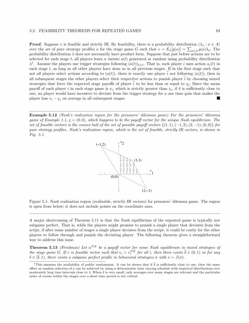
5.2. FEASIBILITY THEOREMS FOR REPEATED GAMES 83
Proof. Suppose v is feasible and strictly IR. By feasibility, there is a probability distribution (λa : a ∈ A)over the set of pure strategy profiles a for the stage game G such that v = Eλ[g(a)] =
∑a∈A g(a)λa. The
probability distribution λ does not necessarily have product form. Suppose that just before actions are to beselected for each stage t, all players learn a variate a(t) generated at random using probability distributionλ1. Assume the players use trigger strategies following (a(t))t≥1. That is, each player i uses action ai(t) ineach stage t, as long as all other players have done so in all previous stages. If in the first stage such thatnot all players select actions according to (a(t)), there is exactly one player i not following (a(t)), then in
all subsequent stages the other players select their respective actions to punish player i by choosing mixedstrategies that force the expected stage payoffs of player i to be less than or equal to vi. Since the meanpayoff of each player i in each stage game is vi, which is strictly greater than vi, if δ is sufficiently close toone, no player would have incentive to deviate from the trigger strategy for a one time gain that makes theplayer lose vi − vi on average in all subsequent stages.
Example 5.12 (Nash’s realization region for the prisoners’ dilemma game) For the prisoners’ dilemmagame of Example 1.1, v = (0, 0), which happens to be the payoff vector for the unique Nash equilibrium. Theset of feasible vectors is the convex hull of the set of possible payoff vectors (1, 1), (−1, 2), (2,−1), (0, 0) forpure strategy profiles. Nash’s realization region, which is the set of feasible, strictly IR vectors, is shown inFig. 5.1.
2
1
(1,1)
(−1,2)
(0,0)
(2,−1)
v
v
Figure 5.1: Nash realization region (realizable, strictly IR vectors) for prisoners’ dilemma game. The regionis open from below; it does not include points on the coordinate axes.
A major shortcoming of Theorem 5.11 is that the Nash equilibrium of the repeated game is typically notsubgame perfect. That is, while the players might promise to punish a single player that deviates from thescript, if after some number of stages a single player deviates from the script, it could be costly for the otherplayers to follow through and punish the deviating player. The following theorem gives a straightforwardway to address this issue.
Theorem 5.13 (Friedman) Let αNE be a payoff vector for some Nash equilibrium in mixed strategies ofthe stage game G. If v is feasible vector such that vi > vNEi for all i, then there exists δ ∈ (0, 1) so for anyδ ∈ [δ, 1), there exists a subgame perfect profile in behavioral strategies σ with v = J(σ).
1This assumes the availability of public randomness. It can be shown that if δ is sufficiently close to one, then the sameeffect as random selection of a can be achieved by using a deterministic time varying schedule with empirical distributions overmoderately long time intervals close to λ. When δ is very small, only averages over many stages are relevant and the particularorder of events within the stages over a short time period is not critical.

84 CHAPTER 5. MULTISTAGE GAMES WITH OBSERVED ACTIONS
Proof. The behavioral strategy profile is constructed as in the proof of Theorem 5.11, but with v replacedby vNE . This strategy profile is subgame perfect because for a subgame such that one player first deviatedfrom the script as some time in the past, all players are to be following repeated play of vNE , which is aNash equilibrium from the subgame. While the Nash equilibrium payoff vector gives punishment for thefirst player to deviate, it is still provides as large a payoff as available for any single player after the triggerevent.
Remarkably, under a minor additional assumption, and with a lot of added complexity in the strategies,Nash’s original realization theorem, Theorem 5.11, can be implemented in subgame perfect equilibria:
Theorem 5.14 (Fudenberg and Maskin [6] realization theorem) Suppose the conditions of Nash’s realizationtheorem, Theorem 5.11 hold, and, in addition, suppose the dimension of the set of feasible payoff vectors isequal to the number of players. Then the conclusion of Theorem 5.11 holds for some subgame perfect profilein behavioral strategies, σ.
See [7] for a proof. The idea of the construction of σ, as in the proof of Theorem 5.11, is to incentivize otherplayers to punish the first player to deviate from the the script of a trigger policy. The problem is it maynot be in the best interest for the players to follow through and do the punishing, because they may in partbe punishing themselves. But then the players acting together can punish players who don’t follow throughto punish the original players, or reward players that do follow through. The proof is easier to prove underthe availability of public randomness, but is still complicated.

Chapter 6
Mechanism design and theory ofauctions
Mechanism design and auctions both address the how to allocate resources in exchange for payments. Mech-anism design focuses on application specific scenarios in which the agents involved (bidders and seller(s))may have some information about each other and there may be substantial flexibility for crafting protocolsfor engagement. The designer of an allocation mechanism is formulating a game, typically in such a way thatsome game theoretic equilibrium of the game, has desirable properties. For example, a seller might wish tomaximize revenue at the Nash equilibrium of an induced game among the bidders. The designer may havein mind specific behaviors of a bidder, given the type or preferences of the bidders.
Auction theory focuses on scenarios with bidders and seller in which the rules of interaction are often selectedfrom among a relatively small set of well known protocols for engagement.
An important class of mechanisms within the theory of mechanism design are seller mechanisms, whichimplement the sale of one or more items to one or more bidders. Some authors would consider all suchmechanisms to be auctions, but the definition of auctions is often more narrowly interpreted, with auctionsbeing the subclass of seller mechanisms which do not depend on the fine details of the set of bidders. Therules of the threes types of auction mentioned above do not depend on fine details of the bidders, such asthe number of bidders or statistical information about how valuable the item is to particular bidders. Incontrast, designing a procedure to sell an item to a known set of bidders under specific statistical assumptionsabout the bidders’ preferences in order to maximize the expected revenue (as in [13]) would be considered aproblem of mechanism design, which is outside the more narrowly-defined scope of auctions. The narrowerdefinition of auctions was championed by R. Wilson [20].
6.1 Vickrey-Clarke-Groves (VCG) Mechanisms
Let C represent a set of possible allocations, or social choices, affecting the players indexed by a finite set I.For example,
• C could be a set of possible locations for a new school in a community.
• Sale of a single item. To model the sale of a single object, such as a license for utilizing a band of
85

86 CHAPTER 6. MECHANISM DESIGN AND THEORY OF AUCTIONS
wireless spectrum, or a painting, C could be equal to I, the set of players, with i ∈ C denoting thatplayer (or bidder) i gets the object.
• Simultaneous sale of a set of objects. To model the simultaneous sale of a set objects, O, with possiblydifferent objects being distributed to different bidders, C could be given by
C = (Ai)i∈I : Ai ⊂ O, Ai ∩Aj = ∅,
with a particular (Ai)i∈I ∈ C denoting that player i gets the objects in Ai for i ∈ I.
Suppose player i has a valuation function vi : C → R, such that vi(c) for c ∈ C is the value player i places onthe allocation c.
Definition 6.1 An allocation mechanism M has the form M = ((Si)i∈I , g, (mi)i∈I), such that
• Si is the set of possible bids of player i. Set S =×i∈I Si, so a bid vector has the form s = (si)i∈I ∈ S.
• g : S → C; g(s) is the allocation or social choice determined by the bid vector s.
• mi : S → R; mi(s) is the amount of money player i has to pay, as determined by the bid vector s.
A set of valuation functions (vi)i∈I and an allocation mechanism M = ((Si)i∈I , g, (mi)i∈I), determines anormal form game (I, (Si)i∈I , (ui)i∈I), where the action sets Si are the sets of possible bids for the mechanism,and
ui(s) = vi(g(s))−mi(s). (6.1)
That is, the payoff of player i is how much player i values the allocation, minus how much player i must pay.This form of payoff function is called quasilinear because it depends linearly on the payment, mi.
The basic goal of mechanism design is to devise an allocation mechanism such that when the players engagein the associated game, the equilibrium of the game defined in some sense (for example, the Nash equilibriumor dominant strategy equilibrium) has some desirable property P. Typically desirable properties could bethat the revenue (sum of payments) is maximized, or the sum of the valuations of the players is maximized (aversion of maximum social welfare). Specifically, for the later example, the (social) welfare for an assignmentc is defined by
W (c) =∑i∈I
vi(c)
and the set of maximum welfare allocations is arg maxc∈CW (c). Another consideration is to make it easyfor players to decide how much to bid, given their valuation functions. Let c∗ = g(sNE), such that sNE
is the Nash equilibrium the players are anticipated to reach. If the mechanism is such that for any profileof valuation functions (vi)i∈I , the allocation c∗ satisfies some property P, then the mechanism is said toimplement property P in Nash equilibria.
The Vickrey-Clarke-Groves (VCG) mechanism, also sometimes called the generalized Vickrey mechanism,implements welfare maximization in weakly dominated strategy equilibrium.
Definition 6.2 (Vickrey-Clarke-Groves (VCG) allocation mechanism) A VCG allocation mechanism for agiven allocation problem is ((Si)i∈I , g, (mi)i∈I) such that the space of bids Si for each player i is the set of

6.1. VICKREY-CLARKE-GROVES (VCG) MECHANISMS 87
possible valuation functions for player i, and allocation and payments are given for a bid vector (vi(·))i∈I by:
c∗ = g(v) ∈ arg maxc∈C
∑i∈I
vi(c), (6.2)
mi(v) = −∑
j∈I,j 6=i
vj(c∗) + ti(v−i) i ∈ I,
where for each i ∈ I, ti(v−i) represents a transfer of money from player i to seller that can depend on thebids of other players but not on the bid of player i.
In words, (6.2) means the VCG allocation rule is to select an allocation that maximizes the sum of thevaluation functions reported in the bids of the players.
Proposition 6.3 (Truthfulness and welfare maximization for VCG mechanisms) Bidding vi (i.e. letting thebid vi be equal to the true valuation function vi) is a weakly dominant strategy for player i for each i ∈ I. Ifall players bid truthfully, the allocation c∗ maximizes the welfare.
Remark 6.4 (a) mi(v) depends directly on the bids v−i of other players, but it depends on vi only throughthe fact the bid vi influences the selection of c∗
(b) Above, v−i represents the vector of bid functions, v−i = (vj : j ∈ I\i), not just the values of thefunctions at some point. So v−i does not depend on the bid, vi, of player i.
(c) A common choice for transfer payments is
ti(v−i) = maxc∈C
∑j∈I\i
vj(c).
That is, ti is taken to be the maximum social welfare of the set of other players, based on their reportedbids. For this choice of ti, the payment function for player i becomes
mi(v) =
maxc∈C
∑j∈I\i
vj(c)
− ∑j∈I\i
vj(c∗). (6.3)
This gives mi(v) ≥ 0, and the payment is the loss in total welfare experienced by the set of other playersdue to the participation of player i in the game.
Proof. The payoff of player i is given by
ui(v) = vi(c∗)−mi(v)
=
vi(c∗) +∑
j∈I\i
vj(c∗)
− ti(v−i) (6.4)
The last term on the righthand side of (6.4) does not depend on the bid vi of player i. Thus, player i wouldlike to submit a bid vi to maximize the sum within the large parentheses on the righthand side of (6.4).That sum is like the social welfare, except it is computed using the bids vj of the other players, which are notnecessarily equal to their true valuation functions. Since the choice of c∗ is given by the VCG allocation rule(6.2), if player i were to report truthfully, that is, if vi = vi, then the allocation rule would be selecting c∗
to maximize the sum within the large parentheses on the righthand side of (6.4). In other words, no matterwhat bids are submitted by the other players, truthful reporting by player i will make the optimization

88 CHAPTER 6. MECHANISM DESIGN AND THEORY OF AUCTIONS
problem solved by the allocation rule the same as the problem of maximizing the payoff of player i. Thus,player i would have no incentive to not report truthfully, no matter what bids are submitted by the otherplayers. Except in trivial cases which we ignore, if player i submits a bid v′i such that v′i 6≡ vi, there is somechoice of bids of the other players such that
arg maxc∈C
vi(c) +∑
j∈I\i
vj(c)
∩ arg maxc∈C
v′i(c) +∑
j∈I\i
vj(c)
= ∅
in which case v′i gives a strictly smaller payoff to player i than truthful bidding.
The last statement of the proposition follows from the form of the VCG allocation rule.
Example 6.5 (Specialization of VCG to Vickrey second price auction) To model the sale of a single itemtake C = I. If bidder i has value vi for the object then vi(c) = vi1c=i. Each bidder i reports a value vi, byreporting the function c 7→ vi1c=i. The VCG allocation rule (6.2) becomes
c∗ = g(v) = arg maxc∈I
∑i∈c
vi1c=i
= arg maxc∈I
vc
and the payment, for the choice of transfer rule in Remark 6.4, is maxc∈I\c∗ vg. That is, the object is soldto a highest bidder and the price is the highest bid of the remaining bidders.
Example 6.6 (VCG for simultaneous sale of objects) Let O denote a set of objects to be distributed amonga finite set of bidders indexed by I. The set of possible allocations is C = (Ai)i∈I : Ai ∈ O, Ai ∩ Aj = ∅.Assume the valuation function of a bidder i, vi, is determined by the set of objects, Ai, assigned to bidder i,and write vi(Ai) to denote the value of set of objects Ai for Ai ⊂ O.The VCG allocation rule is given by
(A∗i )i∈I = g((vi)) = arg min(Ai)∈C
∑i∈I
vi(Ai),
(unfortunately computing the allocation is an NP hard problem) and the payment rule by
mi((vj)) =
max(Aj)j∈I\i
∑j∈I\i
vj(Aj)
− ∑j∈I\i
vj(A∗j ).
A useful interpretation of the payment rule is based on rearranging it to get
mi((vj)) +∑
j∈I\i
vj(A∗j ) = max
(Aj)j∈I\i
∑j∈I\i
vj(Aj). (6.5)
The righthand side of (6.5) is the maximum welfare, based on the reported valuation functions, that canbe achieved without the presence of bidder i. The lefthand side of (6.5) is the welfare that is realized forallocation (A∗j ), with the presence of bidder i, based on the reported valuation functions, and with mi((vj))used instead of vi(A
∗i ) for bidder i. Thus, (6.5) shows that mi((vj)) is the minimum value that player i could
have changed vi(A∗i ) to, and still have been assigned the set A∗i . See the next example for an illustration.

6.2. OPTIMAL MECHANISM DESIGN (MYERSON (1981)) 89
Example 6.7 (Example of Example 6.6) Suppose a VCG mechanism is applied to sell the objects in O =a, b to three bidders. A bidder can buy none, one, or both of the objects. Suppose the values are:
v1(∅) = 0, v1(a) = 10, v1(b) = 3, v1(a, b) = 13
v2(∅) = 0, v2(a) = 2, v2(b) = 8, v2(a, b) = 10
v3(∅) = 0, v3(a) = 3, v3(b) = 2, v3(a, b) = 14
Let’s determine the assignment of objects to bidders and the payments of the bidders, for the VCG mechanismunder truthful bidding.
If both items are allocated to the same bidder, the maximum welfare is 14. A larger welfare is achieved byallocating the items to different bidders, and the maximum of 18 is achieved when bidder 1 is assigned objecta, bidder 2 is assigned object b, and bidder 3 is assigned no object. We’ll calculate the payments using themethod described at the end of Example 6.6. To determine m1, note that the same allocation could have beoccurred if v1(a were reduced to 6, because 6+8 ≥ 14, so m1 = 6. Similarly, the same allocation could haveoccurred if v2(b) were reduced to 4, because 10 + 4 ≥ 14. Finally, m3 = 0. In summary, bidder 1 gets objecta, bidder 2 gets object b, and the payment profile vector is (6, 4, 0). The seller collects a total payment of10. An unsatisfactory aspect of the solution is that bidder 3 could point out (and maybe even file a lawsuit)that he/she bid 14 for the pair a, b and lost, while the mechanism sold a, b for a total payment of only6+4=10.
6.2 Optimal mechanism design (Myerson (1981))
Suppose a single seller has an object to sell and there are n bidders, indexed by a set I. Suppose bidders haveindependent private valuations (Xi)i∈I such that Xi is known to take values in some interval of the form[0, ωi], with probability density function (pdf) fi, and cumulative distribution function Fi. Let 4 denote thespace of probability distributions over I. The seller can use a selling mechanism, whch is a triple (B, π, µ)such that
B =×i∈I Bi is a space of bid vectors, with a typical element written as b = (b1, . . . , bn).
π : B 7→ 4 is the allocation mechanism, specifying the probability distribution used to select which biddergets the object.
µ : B 7→ Rn is the payment rule, such that µi(b) is the (expected) payment of bidder i for bid vector b.
A selling mechanism induces a game of incomplete information among the bidders. Incomplete informationmeans that bidders do not know the types of the other bidders. The types are represented by the Xi’s,which are known by the bidders to be independently distributed, with Xi having known CDF Fi. Thus, asin Section 4.3, we discuss implementation in Bayes-Nash equilibrium.
Following the celebrated paper Myerson [13], we seek a selling mechanism and a specific Bayes-Nash equi-librium for the induced game, such that the expected payoff of the seller is maximized. We assume the sellerhas the option to not sell the object, and in that case the object has value r to the seller, for a fixed constantr, known to the seller and all bidders. It could be r = 0, sometimes called the assumption of free disposal.

90 CHAPTER 6. MECHANISM DESIGN AND THEORY OF AUCTIONS
It could also be r = −∞, meaning the seller must always sell the object to avoid an infinite loss. The payoffof the seller is taken to be
Uo =∑i
µi + r1object not sold.
There are many choices for the space of bid vectors B. For example, each bidder might be required to submita bid in R or a bid in Rd for some d ≥ 1 or in some discrete space or in some space of functions. TheBayes-Nash equilibrium strategies of the bidders are functions mapping their private valuations to the bidspaces, and the strategy of each bidder is supposed to be optimal given the strategies of the other bidders.The large space of possibilities for the bid space B makes it hard to imagine how to get started.
However, there is a natural choice for B. Given the value xi for player i lies in the interval [0, ωi], if theset of possible bids for player i were also equal to [0, ωi], then perhaps it could be arranged that reportingtruthfully by each player is a Bayes-Nash equilibrium, and it is the Bayes-Nash equilibrium that the sellerassumes the players will adopt. Let V =×i∈I [0, ωi], so that V denotes the set of possible value vectors forthe players. A direct mechanism for the set of possible value vectors V is a selling mechanism (B, π, µ) suchthat B = V , or in other words, the space of bid vectors is the space of value vectors. So a direct mechanismfor V has the form (V,Q,M) such that Q : V 7→ 4 (allocation rule) and M : V 7→ Rn (payment rule).
The revelation principle, stated and proved next, is that for the purpose of designing a selling mechanismto maximize the seller’s utility (or to achieve some other desirable property P) at a specified Bayes-Nashequilibrium, there is no loss of optimality in restricting attention to direct selling mechanisms and to truthfulbidding as the specified Bayes-Nash equilibrium.
Proposition 6.8 (Revelation Principle) Let I be a set of n bidders with specified distributions of theirindependent values (fi(xi) : 0 ≤ xi ≤ ωi)i∈I , let (B, π, µ) be a selling mechanism for I, and let β be aBayes-Nash equilibrium for the induced game (so βi : [0, ωi] → Bi for i ∈ I). Also, let V =×i∈I [0, ωi].There is a direct mechanism (V,Q,M) such that reporting truthfully is a Bayes-Nash equilibrium with thesame outcomes under (V,Q,M), as the outcomes of β under (B, π, µ). In other words, the two equilibriagive the same distribution of winner and same payoffs for every x ∈ V.
Proof. The assumption (βi(·))i∈I is a Bayes-Nash equilibrium means, by definition, for any player i andany private value xi of player i,
βi(xi) ∈ arg maxbi
∫V−i
(πi(bi, β−i(x−i))xi − µi(bi, β−i(x−i))) f−i(x−i)dx−i. (6.6)
Taking bi to be of the form bi = βi(x′i), we trivially get the best response value βi(xi) by taking x′i = xi.
Therefore, (6.6) implies:
xi ∈ arg maxx′i
∫V−i
(πi(βi(x′i), β−i(x−i))xi − µi(βi(x′i), β−i(x−i))) f−i(x−i)dx−i. (6.7)
The equivalent direct mechanism is obtained by composing the equilibrium mapping β with the allocationand payment rules of (B, π, µ). In other words, let Q = π β and M = µ β. Then (6.7) becomes:
xi ∈ arg maxx′i
∫V−i
(Qi(x′i, x−i))xi −Mi(x
′i, x−i))) f−i(x−i)dx−i,
which shows bidding truthfully is a Bayes-Nash equilibrium for the game induced by the direct mechanism(V,Q,M). The allocation distribution and the payment vector under (B, π, µ) for the Bayes-Nash equilibrium

6.2. OPTIMAL MECHANISM DESIGN (MYERSON (1981)) 91
β and any given x ∈ V are πβ(x) and µβ(x), respectively, which are the same as the allocation distributionand payment vector, Q(x) and M(x), respectively, for the direct mechanism.
The proof of Proposition 6.6 is summarized in Figure 6.1. In essence, the direct mechanism builds in the
( )
M (x)
π
xβ ( )
.
.
.
n
x 1
µ
n
mechanism
original
direct mechanism
Q (x)
β1
Figure 6.1: Direct mechanism (V,Q,M) is composition of an equilibrium strategy β(·) and original mecha-nism (V, π, µ).
thought process that goes into selecting β. Proposition 6.6 implies we can restrict attention to direct mecha-nisms and focus on truthful bidding as the Bayes-Nash equilibrium in the induced game. The property of bestresponse being truthful bidding is also known in the mechanism design literature as incentive compatibility:
Definition 6.9 (Incentive compatibility (IC)) A direct mechanism (V,Q,M) for a space of value vectorsV with prior distributions specified by pdfs fi or CDFs Fi is incentive compatible if bidding truthfully is aBayes-Nash equilibrium.
The revelation principle still leaves us with huge degrees of freedom for selecting Q and M , but at least itfixes the domains of these functions and it fixes the best response functions of the bidders to be particularlysimple, namely, bidding truthfully. To continue on the path to identifying the optimal mechanism, we shownext Q and incentive compatibility determine the the expected payments, essentially removing M from theoptimization.
If bidder i bids zi he/she gets the object with probability qi(zi), where
qi(zi) =
∫V−i
Qi(zi, x−i)f−i(x−i)dx−i
and he/she expects to pay mi(zi), where
mi(zi) =
∫V−i
Mi(zi, x−i)f−i(x−i)dx−i.
Logically speaking, qi(zi) is just a short hand notation for Qi(zi, f−i), because it is defined by averagingQi(zi, x−i) over all values of x−i using the pdf f−i. Similarly, mi(zi) is shorthand notation for Mi(zi, f−i).Incentive compatibility can now be stated concisely. The mechanism (V,Q,M) is incentive compatible ifand only if, for each i ∈ I and each xi, x
′i ∈ [0, ωi],
U(xi) , qi(xi)xi −mi(xi) ≥ qi(x′i)xi −mi(x′i). (6.8)
Note that (6.8) represents a linear constraint on the functions qi and mi, or on Qi and Mi, for each pair xi, x′i.
It turns out these constraints imply qi is nondecreasing. Moreover, as shown next, the allocation functions

92 CHAPTER 6. MECHANISM DESIGN AND THEORY OF AUCTIONS
(qi) uniquely determine the expected payment functions (mi) up to a constant value. In other words, if twoIC mechanisms for the same distribution of bidder valuations have the same probability allocation functionsqi, then they have the same payment functions up to additive constants.
Proposition 6.10 (Revenue equivalence principle) A direct mechanism (V,Q,M) is IC for a set of priorpdfs f if and only if for each i ∈ I, qi is nondecreasing and mi is determined (up to an additive constant)by:
mi(xi) = mi(0) + qi(xi)xi −∫ xi
0
qi(ti)dti. (6.9)
(If qi is continuously differentiable, (6.9) is equivalent to m′i(xi) = q′i(xi)xi.)
Proof. (only if) Suppose (V,Q,M) is IC for some choice of pdfs (fi)i∈I . Fix i ∈ I. By the definition of IC,for xi, x
′i ∈ [0, ωi]
qi(xi)xi −mi(xi) ≥ qi(x′i)xi −mi(x′i) (6.10)
qi(x′i)x′i −mi(x
′i) ≥ qi(xi)x′i −mi(xi) (6.11)
Adding the respective sides of (6.10) and (6.11) and rearranging yields
(qi(xi)− qi(x′i))(xi − x′i) ≥ 0,
showing qi is a nondecreasing function.
By incentive compatibility, the function Ui(xi) , qi(xi)xi −mi(xi) satisfies:
Ui(xi) = max0≤y≤ωi
qi(y)xi −mi(y), (6.12)
and for xi fixed, the maximum in (6.12) is achieved at y = xi. Thus, Ui is the maximum of a set of affinefunctions. By the envelope theorem, Propostion 6.18, it follows Ui is absolutely continuous, U ′i(xi) = qi(xi)for a.e. xi, and Ui is the integral of its derivative, i.e. Ui(xi) = Ui(0) +
∫ xi0qi(xi)dxi, which is equivalent to
(6.9). (Moreover, Ui is a convex function and for any xi ∈ [0, ωi, ], qi(xi) is subgradient of Ui at any xi.)
(if) Conversely, suppose qi is nondecreasing and mi satisfies (6.9). The definition U(xi) , qi(xi)xi −mi(xi)and (6.9) imply Ui(xi) = Ui(0)+
∫ xi0qi(xi)dxi. Together with the assumption qi is nondecreasing, this implies
Ui is convex and for any x′i ∈ [0, ωi], qi(x′i) is a subgradient of Ui at xi. By definition, that means Ui(x) is
greater than or equal to the linear function agreeing with Ui at x′i with slope qi(x′i). That is, the inequality
in (6.8) holds.
Definition 6.11 (Individually rational) A selling mechanism is individually rational (IR) if any bidder ican bid to obtain a nonnegative expected payoff for any value xi of the bidder.
Proposition 6.12 A direct mechanism that is IC is also IR if and only if mi(0) ≤ 0 for all bidders i.
Proof. For a direct mechanism, the expected payoff of bidder i with value xi and bid x′i is qi(x′i)xi−mi(x
′i).
The worst case value of xi for the bidder is zero, in which case the payoff of the bidder is −mi(x′i). Therefore,
IR holds if and only if there is some choice of x′i such that mi(x′i) ≤ 0. For a direct mechanism with the IC
property, mi is nondecreasing, so the IR property is equivalent to mi(0) ≤ 0.
Given the allocation rule of a direct mechanism, Proposition 6.10 shows the IC property determines theexpected payment functions mi up to additive constants, and Proposition and 6.12 shows the IR property

6.2. OPTIMAL MECHANISM DESIGN (MYERSON (1981)) 93
for an IC payment rule is equivalent to the inequality constraint mi(0) ≤ 0. Therefore, to maximize theexpected payments, or equivalently, to maximize the expected utility of the seller, subject to the IC andIR constraints and a given allocation rule, it is equivalent to using a payment rule satisfying (6.9) withmi(0) = 0 for all i.
Example 6.13 Suppose qi(xi) = xi for 0 ≤ xi ≤ 1, so the probability bidder i gets the object is proportionalto the bid. What is the maximum expected payment function mi subject to the IC and IR constraints? Since qi
is differentiable, (6.9) becomes m′i(xi) = q′i(xi)xi = xi. Solving for mi with mi(0) = 0, yields mi(xi) = (xi)2
2 .This identifies the maximum expected revenue from bidder i for an IC, IR mechanism, given bidder i getsthe object with probability xi for bid xi ∈ [0, 1]. To check the IR property of this solution, note, for example,if the value of the object to the bidder is 0.6, the expected payoff to the bidder, if the bidder bids xi, is
xi(0.6)− (xi)2
2 . This payoff is maximized if the bidder bids truthfully, taking xi = 0.6.
Example 6.14 If qi(xi) = 1 − e−xi for xi ≥ 0, then the expected payment function that maximizes theexpected payment (i.e. revenue to the seller) subject to the IC and IR constraints is is given by m′i(xi) =q′i(xi)xi = xie
−xi and mi(0) = 0, or mi(xi) = 1− (1 + xi)e−xi .
Up to this point, given the selection rule Q, we can determine revenue optimal pricing mechanisms subject tothe IC and IR constraints. The remaining step towards finding the optimal seller mechanism is to determineQ. We view this as a linear optimization problem, given (fi)i∈I where fi is a pdf with support [0, ωi] foreach i ∈ I. Since the mechanism is constrained to be IC, we maximize the payoff of the seller assuming thebidders bid truthfully. Thus, the optimization problem can be written as:
maximize E
[(∑i∈I
mi(Xi)
)+ r1no bidder gets object
]with respect to (Q,M)
subject to IC and IR
Since M is determined by Q and the IC and IR constraints, we can write the objective function in a formdepending only on the distributions of the values and Q. Taking mi(0) = 0, which is optimal subject to theIC constraints, yields mi(xi) = qi(xi)xi −
∫ xi0qi(t)dt.

94 CHAPTER 6. MECHANISM DESIGN AND THEORY OF AUCTIONS
Therefore,
E [mi(Xi)] =
∫ ωi
0
qi(xi)xifi(xi)dxi −∫ ωi
0
∫ xi
0
qi(t)dtf(xi)dxi
(a)=
∫ ωi
0
qi(xi)xifi(xi)dxi −∫ ωi
0
∫ ωi
t
f(xi)dxiqi(t)dt
=
∫ ωi
0
qi(xi)xifi(xi)dxi −∫ ωi
0
(1− Fi(t))qi(t)dt
=
∫ ωi
0
qi(xi)xifi(xi)dxi −∫ ωi
0
(1− Fi(xi))f(xi)
qi(xi)f(xi)dxi
=
∫ ωi
0
ψi(xi)qi(xi)fi(xi)dxi
= E[ψi(Xi)1i gets object
]where
ψi(xi) = xi −1− Fi(xi)fi(xi)
,
and i gets object denotes the event player i gets the object. Equality (a) in the above derivation is obtainedby changing the order of integration over the region shown in Fig. 6.2.
i
0
ω
i
t
ωi
x
Figure 6.2: A key step in the derivation of the optimal selling mechanism is to change the order of integration,for integration over the region shown.
The function ψ(xi) is called the virtual valuation for bidder i. The total expected revenue is the sum ofE [mi(Xi)] over all i, so the mechanism optimization problem reduces to finding the winner selection functionQ to solve:
maxE
[(∑i∈I
ψi(Xi)1i gets object
)+ r1no bidder gets object
](6.13)
with respect to Q
subject to xi 7→ qi(xi) nondecreasing for each i
Ignore, for a moment, the constraint that qi be nondecreasing for each i in the optimization problem (6.13).The allocation mechanism selects which bidder gets the object or to have no bidder get the object, after learn-ing (Xi)i∈I , so the following selection rule minimizes the quantity inside the expectation with probability one.
MAX VIRTUAL VALUATIONselection rule
• Select winner from arg maxi ψi(Xi) if maxi ψi(Xi) ≥ r
• Select no winner if maxi ψi(Xi) < r

6.2. OPTIMAL MECHANISM DESIGN (MYERSON (1981)) 95
Fortunately, in many cases the constraint on the qi’s is satisfied by this rule, making the rule the optimalsolution. Specifically, Myerson defined the mechanism design problem to be regular if ψ(xi) is increasingin xi for each i. If the problem is regular, then the above selection rule satisfies the constraint that qi isnondecreasing for each i. If the problem is not regular, the solution is a bit more complicated, with ψ(xi)
being replaced by functions ψ(xi) that are nondecreasing. Henceforth we assume the mechanism designproblem is regular.
The expected payoff of the seller for the optimal auction is given by
E [maxψ1(X1), . . . , ψn(Xn), r] . (6.14)
The allocation rule as described above is simple, at least once the functions ψi are computed. The abovederivation determines the expected payment functions, namely,
mi(xi) = qi(xi)xi −∫ xi
0
qi(t)dt,
but the expected payment mi(xi) for a bidder i doesn’t depend on whether the player gets the object.Recalling that Mi(x) is the payment of player i given the entire bid vector x ∈ V, any choice of M such that
E [Mi(X)|Xi = xi] = mi(xi) (6.15)
is a valid choice for the revenue optimal mechanism, subject to the IC and IR constraints. Thinking of thesecond price auction suggests a good choice for Mi. Let yi(x−i) denote the minimum bid for player i suchthat player i gets the object (assuming the player gets the object in case of a tie):
yi(x−i) = minzi : ψi(zi) ≥ r and ψi(zi) ≥ ψj(xj) for j 6= i
Then consider the payment rule Mi(x) given as follows:
MIN TO WIN payment rule: Mi(x) = yi(x−i)1i gets object.
Let us verify that this choice of M satisfies (6.15), so indeed it is revenue optimal for the given Q. Ob-serve
qi(xi) = P i gets object|xi = P yi(X−i) ≤ xi .
Therefore, qi is the CDF of the random variable yi(X−i). We use the area rule for expectations of randomvariables, which for a nonnegative random variable Y bounded above by ymax is E [Y ] =
∫ ymax
0P Y > t dt,
to get
E [Mi(X)|Xi = xi] = E[yi(X−i)1yi(X−i)≤xi
]=
∫ xi
0
Pyi(X−i)1yi(X−i)≤xi > t
dt
=
∫ xi
0
P t < yi(X−i) ≤ xi dt
=
∫ xi
0
(qi(xi)− qi(t))dt
= qi(xi)xi −∫ xi
0
qi(t)dt = mi(xi) (6.16)
We summarize the above results as a proposition.

96 CHAPTER 6. MECHANISM DESIGN AND THEORY OF AUCTIONS
Proposition 6.15 (Myerson(1982)) Given prior pdfs fi over [0, ωi] for the independent private values ofbidders indexed by i in I and a known reserve value r of the seller, the seller’s expected payoff at Bayes-Nashequilibrium over all IR seller mechanisms is maximized by the direct mechanism (V,Q,M) with Q definedby the MAX VIRTUAL VALUATION selection rule and M defined by the MIN TO WIN payment ruleidentified above, with the corresponding equilibrium being truthful bidding (so the mechanism is IC).
Remark 6.16 The reserve value for bidder i is given by ri = infzi : ψ(zi) ≥ r. bidder i can’t win ifhis/her bid is less than ri. If xj < rj for all bidders, the seller does not allocate the object to any bidder.
Example 6.17 (Second price auction–alternative verification of IC and IR properties, and constrained op-timality) Let us consider some of the implications of this section for second price auctions. As discussedin Examples 1.4 and 6.5, a second price auction is a direct mechanism (V,Q,M) such that Q(x) selects awinner i∗ with i∗ ∈ argmaxi xi and Mi(x) = wi1i∗=i, where wi = maxj∈I\i xj .
As noted in Example 1.4, bidding truthfully is a weakly dominant strategy for any bidder. Truthful biddingis thus also a Bayes-Nash equilibrium for given prior pdfs, (fi)i∈I , on the values of the bidders. That is,the second price auction is IC. It is also IR, because a bidder can avoid negative payoffs by bidding zero.Moreover, mi(0) = 0 for any bidder, because a player i that bids 0 gets the object with probability zero. Whilewe have thus directly verified the payment rule is IC and mi(0) = 0, let’s verify it a second way by appealingto the revenue equivalence principle, Proposition 6.10.
Consider the game from the perspective of some bidder i. Let Wi be a random variable representing thehighest bid of the other bidders. Then if bidder i bids xi, the bidder i gets the object with probabilityqi(xi) = P Wi ≤ xi . That is, qi is the CDF of Wi. As in the derivation of (6.16) above, we find theexpected payment functions for the second price auction are given by:
mi(xi) = E [Mi(X)|Xi = xi]
= E[Wi1Wi≤xi
]= xiqi(xi)−
∫ xi
0
qi(t)dt.
Thus Proposition 6.10 implies the second price auction is IC, and we also see mi(0) = 0.
If the mechanism design problem is symmetric, so the pdfs for the values of all bidders are the same, the ψiis the same for all bidders. If the problem is also regular, then ψi is strictly increasing. Finally, if sellermust sell the object (i.e. r = −∞, then the object goes to the highest bidder in the optimal mechanism. Sincethis allocation is the same as the allocation of the second price auction, the revenue equivalent principle,Proposition 6.10, implies the second price auction is revenue optimal in the symmetric case when the biddermust sell.
If the design problem is not symmetric, then the functions ψi are not all the same, and choosing i to maximizeψ(Xi) is different from choosing i to maximize Xi. Therefore, the second price auction is not revenue optimalin that case.
6.3 Appendix: Envelope theorem
A useful class of functions are the absolutely continuous functions. A function f : [a, b] → R is absolutelycontinuous if for any ε > 0, there exists δ > 0 such that
∑ni=1 |f(t′i)− f(ti)| ≤ ε, for any finite collection of
nonoverlapping intervals (ti, t′i) in [a, b]. For example, if f is continuous and piecewise differentiable, then

6.3. APPENDIX: ENVELOPE THEOREM 97
it is absolutely continuous. An absolutely continuous function is differentiable almost everywhere (i.e. at allpoints of [a, b] except for a set of Lebesgue measure zero.) Also, a function f : [a, b] → R is an indefiniteintegral, meaning it can be expressed as f(x) = f(a) +
∫ xag(t)dt (using Lebesgue integration), if and only if
f is absolutely continuous. If f is absolutely continuous, the integrand in the indefinite integral can be anymeasurable version of f ′(t). Here, f ′(t) is the derivative of f at t if f is differentiable at t and can be definedarbitrarily otherswise, subject to being a measurable function. (See [17] for proofs.)
Proposition 6.18 (Milgrom and Segal [11]) Let F be a set of differentiable and absolutely continuousfunctions on some interval [a, b]. Let F∗(t) = arg maxf∈F f(t), and suppose F∗(t) 6= ∅ for almost every
t ∈ [a, b]. Also, suppose there is a function h : [a, b] → R such that∫ ba|h(t)|dt < ∞ and, for any f ∈ F ,
|f ′(t)| ≤ h(t) almost everywhere. Let V (t) = supf(t) : t ∈ F for t ∈ [a, b]. Then V is absolutely continuous,and V ′(t) = f ′(t) for all f ∈ F∗(t), for almost every t ∈ [a, b].
Proof. For any interval (t, t′) ⊂ [0, 1], |V (t) − V (t′)| ≤ supf∈F |f(t′) − f(t)| = supf∈F∫ t′t|f ′(s)|ds ≤∫ t′
th(t)dt, implying that V is absolutely continuous. Therefore,V is differentiable for almost every t. For
any t ∈ (a, b), if V is differentiable at t and V (t) = f(t) for some f ∈ F , then it must be that V ′(t) = f ′(t)because f ≤ V over [a, b], implying the last part of the proposition.
Example 6.19 Let g : R→ R∪+∞ be a convex function and let V denote its Legendre-Fenchel transform:V (t) = supθ∈R θt−g(θ), and let θ∗(t) ∈ arg maxθ θt−g(θ). Suppose θ∗ is well defined and bounded over someinterval t ∈ [a, b]. Then V is absolutely continuous over [a, b] and V ′(t) = θ∗(t) for almost every t ∈ [a, b].This fact follows from Proposition 6.18 by taking F to be the set of functions of the form f(t) = θt − g(θ)for |θ| ≤ sup|θ∗(t)| : a ≤ t ≤ b, and h(t) ≡ sup|θ∗(t)| : a ≤ t ≤ b.This result can be derived another way under more restrictive assumptions, as follows. Note that V (t) =θ∗(t)t− g(θ∗(t)). If g and θ∗(t) were differentiable we could apply the chain rule of differentiation to obtainV ′(t) = θ∗(t) + (t− g′(θ∗(t)))θ∗′(t) = θ∗(t), where we use the fact t− g′(θ∗(t)) = 0 because of the definitionof θ∗(t).
Proposition 6.18 is limited to functions on R, but otherwise it is rather general. Various envelope theoremsfor functions with domains of dimension greater than one follow from Proposition 6.18 by considering one-sided directional derivatives of the function in various directions from a given point, or by considering therestriction of such functions to line segments. One such result is the following proposition.
Proposition 6.20 Let F be a set of functions f : D → R, where D is an open subset of Rd. Let V (t) =supf(t) : t ∈ F for t ∈ D. Suppose the functions in F and the function V are continuously differentiable.Let F∗(t) = arg maxf∈F f(t) for t ∈ D and suppose F∗(t) 6= ∅ for all t ∈ D. Then for any t ∈ D,∇V (t) = ∇f(t) for all f ∈ F∗(t).

98 CHAPTER 6. MECHANISM DESIGN AND THEORY OF AUCTIONS

Chapter 7
Introduction to Cooperative Games
7.1 The core of a cooperative game with transfer payments
Definition 7.1 A cooperative game with transfer payments consists of (I, (v(S))S⊂I), where
• I is a finite set of players; a subset S of I is a coalition and the set I of all players is the grandcoalition.
• v is the coalitional value function; v(S) is the value or worth of a coalition S. It is assumed v(S) ∈ Rfor any coalition S, and v(∅) = 0.
Often in strategic form games, a group of players can get better payoffs for themselves by cooperation. Fora coalition S, v(S) represents the value the players in the coalition could achieve among themselves, withoutparticipation by the players in I\S. A central question addressed in the theory of cooperative games is whendoes there exist a profile of payoffs to the players so that all players have incentive to cooperate within thegrand coalition, I, rather than having some subset of players wanting to break away and cooperate insteadwithin a smaller coalition.
Mathematically, the question is whether the core of the game is nonempty, where the core is defined asfollows. A payoff profile is a vector of real numbers, x = (xi)i∈I , such that xi is the payoff to player i. Letx(S) represent the sum of payoffs for a coalition S : x(S) =
∑i∈S xi.
Definition 7.2 A payoff profile x is feasible if x(I) = v(I). (In other words, the sum of payoffs is equal tothe value of the grand coalition.)
The core of the cooperative game (I, v) with transferable payoffs is the set of payoff profiles (xi)i∈I such that
(1) x is feasible, and
(2) x(S) ≥ v(S) for all coalitions S.
The feasibility assumption means that the payoffs should be covered by the value of the grand coalition. Inother words, there is no subsidy provided to the grand coalition to incentivize the players to cooperate. Thecondition x(S) ≥ v(S) means that if the players in the coalition S decided to break away from the otherplayers, their value v(S), which perhaps they could distribute among themselves, would be less than theirsum of payoffs x(S) if they cooperate within the grand coalition.
99

100 CHAPTER 7. INTRODUCTION TO COOPERATIVE GAMES
Next we identify a necessary condition for the core to be nonempty. A partition of I is a set of subsetsS1, . . . , SK of I such that I = ∪Kk=1Sk and Sj ∩Sk = ∅ if j 6= k. Each of the sets Sk in a partition is calleda block of the partition.
Definition 7.3 A cooperative game (I, v) is cohesive if
v(I) ≥K∑k=1
v(Sk) (7.1)
for every partition S1, . . . , SK of I.
Equality holds in (7.1) for the partition with only a single block equal to I, because then K = 1 and
S1 = I. So cohesiveness is equivalent to the condition v(I) = max∑Kk=1 v(Sk), where the maximum is over
all partitions S1, . . . , SK of I.
If the game is not cohesive, there exists a partition S1, . . . , SK such that for any feasible payoff profile,∑k x(Sk) = x(I) = v(I) <
∑k v(Sk), implying that x(Sk) < v(Sk) for some block Sk. Therefore, the core
of the game is empty if the game is not cohesive. Intuitively, if the game is not cohesive, the players of thegrand coalition in aggregate could generate more total value by working within smaller coalitions, so theremay be no point to make them cooperate. Of course if some external agency would like to incentivize theplayers to cooperate in the grand coalition, it could offer to pay a subsidy if all the players agree to cooperatein the grand coalition, effectively increasing the value of v(I), to result in a cohesive game.
In summary, cohesiveness is necessary for the core to be nonempty. Henceforth, we restrict attention tocohesive games. As illustrated in the next example, cohesiveness is not sufficient for the core to be nonempty.However, a theme in this chapter is that for games with many players with enough mixing among them,cohesiveness is typically sufficient for a nonempty core.
Example 7.4 (three player majority game) Consider the coalition game with I = 1, 2, 3 and v definedby v(i) = 0 for all i, v(1, 2) = v(1, 3) = v(2, 3) = α for some fixed α with 0 ≤ α ≤ 1, andv(1, 2, 3) = 1. The game is cohesive. A vector (x1, x2, x3) is in the core if
xi ≥ v(i) = 0
xi + xj ≥ v(i, j) = α i 6= j
x1 + x2 + x3 = 1
Thus, if x is in the core,
1 = x1 + x2 + x3 =(x1 + x2) + (x1 + x3) + (x2 + x3)
2≥ 3α
2.
So the core is empty if α > 23 . If 0 ≤ α ≤ 2/3, the core is not empty. For example, it contains
(13 ,
13 ,
13
). It
also contains (1− α, α, 0) if 0 ≤ α ≤ 12 , and (1− α, 1− α, 2α− 1) if 1
2 ≤ α ≤23 .
Example 7.5 (production economy) Let I = c ∪W , where c represents a factory owner, and W is a setof m workers, for some m ≥ 1. In order for a coalition to have positive worth, it must include the owner andat least one worker, because both the factory and at least one worker are needed for production. Suppose theworth of a coalition consisting of the owner and k workers is f(k), where f : [m]→ R is such that f(0) = 0, fis monotone increasing, and its increments f(k+1)−f(k) are nonincreasing in k over 0 ≤ k ≤ m−1. In other

7.1. THE CORE OF A COOPERATIVE GAME WITH TRANSFER PAYMENTS 101
words, if Sw is a set of workers, v(Sw) = 0 and v(c∪Sw) = f(|Sw|). The assumption f has nonincreasingincrements means that if a worker is added to a coalition that includes the owner, the resulting increase inworth of the coalition is a nonincreasing function of the number of other workers.
Let’s find the core of this game. A typical element of the core is a payoff profile of the form (xc, x1, . . . , xm),and the core constraints are (using Sw to denote arbitrary sets of workers):
xc + x1 + · · ·+ xm = f(m) (7.2)
xc +∑i∈Sw
xi ≥ f(k) if |Sw| = k 1 ≤ k ≤ m (7.3)
xi ≥ 0 i ∈ I = c ∪W (7.4)
Constraint (7.3) for k = m− 1 requires xc +∑j∈W\i xj ≥ f(m− 1) for any worker i, which combined with
(7.2) implies xi ≤ f(m)− f(m− 1) for any i. In other words, the payoff to any worker i must be less thanor equal to the marginal value of the last worker joining the grand coalition. Thus, the core is contained inthe set
(xc, x1, . . . , xm) : 0 ≤ xi ≤ f(m)− f(m− 1) for i ∈ [m] and xc + x1 + · · ·+ xm = f(m) (7.5)
However, it is easy to check that any element in the set in (7.5) satisfies the core constraints (7.2)-(7.4), so(7.5) gives the core of the game. The payoff profile in the core that maximizes the payoffs to the workersis xc = f(m) −m(f(m) − f(m − 1)) and xi = f(m) − f(m − 1) for 1 ≤ i ≤ m. The payoff profile in thecore that minimizes the payoffs to the workers is xc = f(m) and xi = 0 for 1 ≤ i ≤ m. In other words, theworkers get zero payoff.
Definition 7.6 Let v = (v(S) : S ⊂ I) with v(∅) = 0.
(a) v is supermodular if v(S ∪ T ) + v(S ∩ T ) ≥ v(S) + v(T ) for all S, T ⊂ I.
(b) v is superadditive if v(S ∪ T ) ≥ v(S) + v(T ) for all S, T ⊂ I such that S ∩ T = ∅.
Remark 7.7 (a) Clearly supermodularity implies superadditivity.
(b) If the coalitional value function v of a cooperative game (I, v) is superadditive, the game is cohesive.
(c) The following is equivalent to supermodularity: v(A ∪ C) − v(A) ≥ v(B ∪ C) − v(B) if A ∩ C = ∅ andB ⊂ A. In other words, the increase in worth for adding C to A is greater than or equal to the increase inworth for adding C to a subset of A. To see the equivalence to the original definition of supermodularity,let S = A and T = B ∪ C.
The following shows that cooperative games (I, v) with supermodular coalitional value functions v have anonempty core, and certain elements of the core are easy to identify.
Proposition 7.8 If (I, v) is a cooperative game such that v is supermodular (some authors call such coopera-tive games convex), then the core is nonempty. Moreover, for any permutation π of I, let Sk = π1, . . . , πkbe the set consisting of the first k elements of π, for 1 ≤ k ≤ n. Then the payoff vector x defined byxπi = v(Si)− v(Si−1) is in the core. (An equivalent expression for x is xπi = v(Si−1 ∪ xπi)− v(Si−1), sothe payoffs are the marginal increases in value as players join to form the grand coalition one at a time inthe order of π.)
Proof. Since the players can be relabeled if necessary, assume without loss of generality that πi = i for1 ≤ i ≤ n. Note that v(I) =
∑ni=1 v(Si) − v(Si−1) =
∑ni=1 xi, so x is feasible. The remaining requirement,

102 CHAPTER 7. INTRODUCTION TO COOPERATIVE GAMES
v(R) ≥ x(R) for any coalition R, is proved as follows. Suppose R = i1, . . . , iq such that i1 < . . . < iq. Bythe supermodularity of v and Remark 7.7(c),
v(R) =
q∑j=1
v(ij ∪ i1, . . . , ij−1)− v(i1, . . . , ij−1)
≤q∑j=1
v(ij ∪ Sij−1)− v(Sij−1)
=
q∑j=1
xij = x(R).
Proposition 7.9 (Bondareva-Shapley theorem) The core of a cooperative game (I, v) is nonempty if andonly if the optimal value for the following linear optimization problem is v(I) :
(D) max∑S⊂I
v(S)λS
over λ = (λS)S⊂I , subject to
λS ≥ 0 for all S ⊂ I,∑S:i∈S
λS ≤ 1 for all i ∈ I
(The choice λS = 1S=I shows that the optimal value of (D) is greater than or equal to v(I), so the optimalvalue of the problem being equal to v(I) is the same as the optimal value being less than or equal to v(I).)
Remark 7.10 If the variables λ in the optimization problem of Proposition 7.9 were restricted to be integer,hence binary, valued, then the optimal value of the problem is v(I) by the cohesiveness assumption. Thus,the problem is a fractionalized version of an integer programming problem connected with cohesiveness. Thevariable λS can be interpreted as the fraction that coalition S is active, and every agent in S needs to devotea fraction λS of his/her effort to cooperation within S. The last constraint in problem (D) means the sum ofthe fractional efforts of any agent i is at most one.
Proof. The core of a cooperative game (I, v) is nonempty if and only if the optimal value for the followinglinear optimization problem (P) is v(I) :
(P ) min∑i∈I
xi
over x, subject to∑i∈S
xi ≥ v(S) for all S ⊂ I,
because the constraints of this problem, along with the condition∑i∈I xi = v(I), are exactly the core
constraints. In other words, if the value of (P) is v(I), then the core is the set of solutions of (P), and if thecore is nonempty, any v in the core is a solution of (P) and the value is v(I).
The proof is completed by showing that the optimization problem (D) in the statement of the propositionis the linear programming dual of problem (P). (Recall that strong duality holds for linear programmingproblems.)

7.1. THE CORE OF A COOPERATIVE GAME WITH TRANSFER PAYMENTS 103
Example 7.11 Consider the three player majority game of Example 7.4 with 0 ≤ α ≤ 1. The vector λS = 12
if |S| = 2 and λS = 0 otherwise, is feasible for the problem (D) in the Bondareva-Shapley theorem. Therefore,the theorem shows that the core being nonempty requires 1
2v(1, 2)+ 12v(2, 3)+ 1
2v(3, 1) ≤ 1, or 3α/2 ≤ 1,or α ≤ 2
3 .
Given the definition of cooperative game, it is reasonable to assume that v is superadditive. If v is notsuperadditive, we could consider the least superadditive majorant, defined as follows.
Definition 7.12 Given a function (v(S) : S ∈ I), the least superadditive majorant of v is the minimumfunction v such that v is superadditive and v(S) ≥ v(S) for all S. It is given by
v(S) = max
∑k
v(Sk) : S1, . . . , SK is a partition of S
.
If v is cohesive then v and v have the same core. As seen above, if v is not cohesive, then the core of v isempty. In such case it may still be of interest to consider the least superadditive majorant v instead, andsince v is cohesive, it could possibly have a nonempty core.
Given a cooperative game (I, v) and an integer k ≥ 1, the k-fold replicated game is defined as follows. Theset of players is I ′ = I × 1, . . . , k, with k players of each type from the original game. For S′ ⊂ I ′, let
w(S′) =
w(S) if for some S ⊂ I, |S′| = |S|, and there is one player in S′ for each type in S
mini∈I v(i) else (i.e. if S′ has at least two players of the same type)
and let v′ be the least superadditive majorant of w. Note that (I ′, v′) is a cohesive game because v′ issuperadditive.
Proposition 7.13 (Koneko & Weiders(1982)) For some integer K, the core of the k-fold replicated gameis nonempty for every k that is a positive multiple of K.
Proof. By the Bondereva-Shapley theorem and the fact that (I ′, v′) is a cohesive game, the core of (I ′, v′)is nonempty if there is a solution to the dual problem for (I ′, v′) such that the λ’s are binary valued. Thevalue of the dual problem for (I ′, v′) is K times the value of the dual problem for (I, v). Since the dualproblem for (I, v) is a linear optimization problem such that the constraints involve only integer values andinteger coefficients, a standard result in the theory of linear programming implies there exists a solution λ∗
of the dual problem for (I, v) with rational entries. Thus, for some integer K ≥ 1, λ∗S = kSK for integers
(kS : S ⊂ I). This implies that there is a solution to the dual problem for (I ′, v′) with binary values of theλ’s, which, as noted above, completes the proof.
Example 7.14 Consider the three player majority game of Example 7.4 with 0 ≤ α ≤ 1. The two-foldreplicated game has players I ′ = 1, 1′, 2, 2′, 3, 3′, v′(I ′) = 3α = w′(1, 2) + w(3, 1′) + w(2′, 3′). Notethat v′(I ′) is not simply 2v(I). It is easily checked that
(α2 ,
α2 ,
α2 ,
α2 ,
α2 ,
α2
)is in the core of (I ′, v′).
Example 7.15 (The core for simultaneous sale of objects) Examples 6.6 and 6.7 are about use of the VCGmechanism for simultaneous sale of objects. Here we model the sale as a cooperative game and focus on thecore. Let O denote a set of objects to be distributed among a finite set of bidders indexed by I. The set of

104 CHAPTER 7. INTRODUCTION TO COOPERATIVE GAMES
possible allocations is C = (Ai)i∈I : Ai ⊂ O,Ai ∩Aj = ∅. Assume the valuation function of a bidder i, vi,is determined by the set of objects, Ai, assigned to bidder i, and write vi(Ai) to denote the value of set ofobjects Ai to bidder i, for Ai ⊂ O.To model this scenario as a cooperative game we take the seller to also be a player, because it doesn’t makesense to let any one of the bidders simply break away on his/her own and be able to get whatever bundle ofobjects he/she would like. To be definite, let us suppose the value of any set of objects to the seller is zero.Thus consider the cooperative game with set of players I ′ = 0∪ I = 0, . . . , n, where player 0 is the seller.The coalitional value function v(S) is given by:
v(S) =
maxpartitions (Aj)j∈S\0
∑j∈S vj(Aj) if 0 ∈ S
0 else(7.6)
A payoff vector x is in the core if and only if v(S) ≤ x(S) for all S and x(I) = v(I). The core is not empty.For example, x0 = v(I ′) and xi = − for 1 ≤ i ≤ n (i.e. all value goes to the seller) is in the core.
Let’s find the core for the specific case of Example 6.7: O = a, b and three bidders with value functions:
v1(∅) = 0, v1(a) = 10, v1(b) = 3, v1(a, b) = 13
v2(∅) = 0, v2(a) = 2, v2(b) = 8, v2(a, b) = 10
v3(∅) = 0, v3(a) = 3, v3(b) = 2, v3(a, b) = 14
The nonzero values of the coalition value function are given by:
v(0, 1, 2, 3) = 18
v(0, 1, 2) = 18, v(0, 1, 3) = 14, v(0, 2, 3) = 14
v(0, 1) = 13, v(0, 2) = 10, v(0, 3) = 14
The core constraints are thus:
xi ≥ 0 for 0 ≤ i ≤ 3
x0 + x1 + x2 + x3 = 18
x0 + x1 + x2 ≥ 18
x0 + x1 + x3 ≥ 14
x0 + x2 + x3 ≥ 14
x0 + x1 ≥ 13
x0 + x2 ≥ 10
x0 + x3 ≥ 14
The first three lines of these constraints imply x3 = 0, and the constraints on the fourth and fifth lines areredundant because of the positivity constraints and the constraint x0 + x3 ≥ 14. Thus, the core constraintssimplify to:
x0 ≥ 14
x1, x2 ≥ 0
x3 = 0
x0 + x1 + x2 = 18
7.2. MARKETS WITH TRANSFERABLE UTILITIES 105
In words, if x is in the core, the sum of the values must be 18 and at least 14 units of value must be allocatedto the seller. The remaining 4 units of value can be shared arbitrarily among the seller and the first twobidders.
Recall that the VCG allocation is to sell item a to bidder 1 and item b to bidder 2 for the payment vector(6, 4, 0). Thus, the payoff vector for the VCG allocation and payment rule is xV CG = (10, 10− 6, 8− 4, 0) =(10, 4, 4, 0). Thus, the VCG outcome is not in the core. Selecting an allocation in the core eliminates theproblem mentioned in Example 6.7, that bidder 3 bid more than the amount charged by the seller, but didnot get the object. However, replacing the VCG outcome by an outcome in the core breaks the incentivecompatibility property of the VCG mechanism.
7.2 Markets with transferable utilities
An important family of cooperative games are market games. A market is a 4-tuple M = (I, `, (wi), (fi))consisting of
• I, a set of n agents for some finite n.
• ` ≥ 1, the number of goods The goods are assumed to be divisible, such as water, oil, steel, data rate
• wi ∈ R`+, the initial endowment of agent i, for i ∈ I. The entries of wi are the amounts of each goodagent i has initially.
• fi : R`+ → R is a production/utility/happiness function for agent i ∈ I, assumed to be increasing,continuous, and concave.
A market induces a cooperative game (I, v) with coalitional value function v defined by
v(S) , max
∑i∈S
fi(zi) : zi ∈ R`+,∑i∈S
zi =∑i∈S
wi
. (7.7)
The idea is that the agents can benefit by exchanging goods and money among themselves. The value, v(S),of a coalition S ⊂ I is the maximum sum of utilities that the agents within the coalition S could achieveby redistributing their initial endowments among themselves. Player i obtains a profile of goods zi for eachi ∈ S. If (Sk)1≤k≤K is a partition of I, then
∑Kk=1 v(Sk) is the maximum sum of utilities that can be achieved
by redistribution of initial endowments, subject to conservation of the amount of each good within each blockSk. The induced cooperative game is cohesive because the maximum sum of utilities over all players can beachieved by unrestricted redistribution of the initial endowments, conserving only the total amount of eachgood within the grand coalition I.
The value v(I) is the maximum social welfare that can be achieved by redistribution of the initial endowments.The optimization problem defining v(I) is convex. To gain insight, let us consider the problem in detail andidentify the dual optimization problem. Let p ∈ R` denote a vector of multipliers associated with theconservation of goods constraint,
∑i∈I zi =
∑i∈I wi. The entries of p can be interpreted as unit prices for
the goods, in which case a payoff vector for the agents is given by (fi(z∗i )− p(z∗i −wi))i∈I , where p(zi −wi)
is the inner product of p and (zi − wi) (i.e. pT (zi − wi)).

106 CHAPTER 7. INTRODUCTION TO COOPERATIVE GAMES
The optimization problem defining v(I) is the following.
max∑i∈I
fi(zi)
with respect to z
subject to z ≥ 0 and∑i∈I
zi =∑i∈I
wi.
This convex optimization problem satisfies the Slater condition if∑i∈I wi > 0 coordinatewise, in which case
strong duality holds. The Lagrangian function is
L(z, p) =∑i∈I
fi(zi)−∑i∈I
p(zi − wi).
The dual optimization problem is
minp∈R`
(∑i∈I
maxzi≥0fi(zi)− p(zi − wi)
). (7.8)
The solution (p∗, z∗) is called a competitive equilibrium (or Walrasian equilibrium) in classical economics. Inother words, such an equilibrium satisfies:
• z∗ is a feasible allocation:∑i∈I z
∗i =
∑i∈I wi.
• z∗i ∈ arg maxzi≥0fi(zi)− p∗(zi − wi).
The payoff vector x∗ for a competitive equilibrium (p∗, z∗) is given by x∗i = fi(z∗i )−p∗(z∗i−wi). If the functions
fi are strictly concave then the competitive equilibrium is unique. Also in that case, by the envelope theorem,the gradient of the ith term of the sum in (7.8) is zi(p) − wi, so the condition
∑i∈I z
∗i =
∑i∈I wi implies
the gradient of the dual objective function at p∗ is zero.
A competitive equilibrium is an equilibrium for price-taking agents, and the prices are adjusted so that thesupply of each good matches the demand. To expand on this point, suppose agent i is presented with thevector of unit prices p∗ for the various goods, and has the option of selecting a vector zi ∈ R`+ representinghow much of each good the agent will end up with, by possibly selling some of the goods in his/her initialendowment wi and possibly buying some other goods. The condition z∗i ∈ arg maxzi≥0fi(zi)− p∗(zi−wi)means that z∗i is the best response for agent i, under the assumption that the price vector p∗ does not dependon the agent’s choice of zi. The feasibility condition for the competitive equilibrium means the price vectorp∗ is adjusted so that, under the assumption of price taking agents, the total supply of each good is equalto the demand.
The opposite of a price-taking agent is a strategic agent, who takes into account the impact of his/her choiceof zi on the price charged. Such strategic behavior of an agent is rational if the agent controls a significantportion of the market, in other words, if the agent has significant market power. The notion of competitiveequilibrium, in contrast, is most relevant for large markets, with a large number of agents, such that thechoice of each individual agent has only a small impact on any other agent.
Proposition 7.16 (Payoff vectors for competitive equilibria are in the core) The payoff vector for anycompetitive equilibrium of the market is in the core of the induced cooperative game. In particular, the coreis nonempty.

7.2. MARKETS WITH TRANSFERABLE UTILITIES 107
Proof. Let S ⊂ I. It must be shown that∑i∈S x
∗i ≥ v(S), where v is defined by (7.7). Equivalently, by the
definition of the x∗i ’s and v, it suffices to show that for any (zi)i∈S with∑i∈S zi =
∑i∈S wi,∑
i∈Sfi(z
∗i )− p∗(z∗i − wi) ≥
∑i∈S
f(zi).
However, this follows from the fact that for each i, fi(z∗i )− p∗(z∗i − wi) ≥ f(zi)− p∗(zi − wi), and the fact∑
i∈S p∗(zi − wi) = 0 (which follows from
∑i∈S zi =
∑i∈S wi).
Example 7.17 (Example of a market M with transferable payments) I = 1, 2, ` = 1, w1 = w2 = 1,f1(z) = ln z and f2(z) = 4 ln z. We shall find the core and the competitive equilibrium. First, the coalitionalvaluation function v is identified. As always, v(∅) = 0. If there is only one player then no transfer of goodsis possible, so v(1) = f1(w1) = ln(1) = 0 and v(2) = f2(w2) = 4 ln(1) = 0. Finally,
v(1, 2) = maxz1,z2≥0,z1+z2≤2
(ln z1 + 4 ln z2) = ln(0.4) + 4 ln(1.6) ≈ −0.9163 + 1.8800 = 0.9637.
The core constraints are xi ≥ v(i) = 0 for i ∈ 1, 2, and x1 + x2 = v(1, 2), so, geometrically speaking,the core is the line segment in R2 with endpoints (v(1, 2), 0) and (0, v(1, 2)). The efficient allocation is(z∗1 , z
∗2) = (0.4, 1.6), which entails the transfer of 0.6 units of good from agent 1 to agent 2. The competitive
equilibrium price p∗ is given by p∗ = f ′i(z∗i ) = 1
0.4 = 41.6 = 2.5. Under p∗, agent 2 pays (0.6)(2.5) = 1.5 to
agent 1. The payoff vector is thus x∗ = (ln(0.4) + 1.5, 4 ln(1.6)− 1.5) ≈ (0.6836, 0.3800), which is a point inthe core, as required by Proposition 7.16.
A clean model for large markets is to start with an exchange market M = (I, `, (wi), (fi)) and an integer kand consider the market kM obtained by k-fold replication of M. Then I indexes the types of the agents inkM. The market kM has k players of each type, wi is the endowment of goods of each type i agent, andfi : R`+ → R+ is the production/utility/happiness function for each type i agent. The market kM is not thesame as k-fold replication of the corresponding cooperative game defined above, because even if a coalitionS in kM has more than one agent of a given type, all the agents in the coalition can exchange goods amongthemselves.
Given a coalition S in kM, let yi denote the number of agents of type i in S. Then y = (yi)i∈I ∈ 0, . . . , kI .Since all agents of the same type have the same production function, v(S) is determined by y, so we candefine γ(y) to equal v(S). In particular, the grand coalition of M , I, corresponds to y = 1, were 1 is thevector of all ones, so v(I) = γ(1). Let x ∈ RI , and for k ≥ 1 let x(k) denote the payoff vector for kM suchthat each agent of type i gets payoff xi. By abuse of notation, we say that x is a payoff vector for kM andit is in the core of kM if x(k) is in the core of kM. With this convention, the value of the grand coalition inkM is kv(I) = ky(1), and if (p∗, z∗) is a competitive equilibrium for M with payoff vector x∗, then (p∗, z∗)can also be considered to be a competitive equilibrium for kM with payoff vector x∗. In that case, z∗i isconsidered to be the final good profile for an agent of type i, and x∗i is the payoff of an agent of type i.
Example 7.18 (Let M be the market of Example 7.17. Let’s find the vectors x = (x1, x2) in the core of 2M(the k-fold market kM for k = 2). The calculations in Example 7.17 imply γ(0, 0) = γ(1, 0) = γ(0, 1) = 0and γ(1, 1) = 0.9637, giving the constraints xi ≥ 0 and x1 + x2 ≥ 0.9637. Since γ(2, 2) = 2γ(1, 1), thefeasibility constraint for 2M is 2x1 + 2x2 = γ(2, 2), which is the same as the feasibility constraint for M :x1 + x2 = 0.9637. There are two types of coalitions in 2M not in M , corresponding to y = (2, 1) andy = (1, 2), consisting of three agents: two of one type and one of another type. We can assume without loss

108 CHAPTER 7. INTRODUCTION TO COOPERATIVE GAMES
of optimality that players of the same type get the same final allocation of goods (e.g. if z′11 and z′12 are theprofiles of goods obtained by two agents of type 1, they can be assumed to be equal). Therefore,
γ(2, 1) = maxz′11,z
′12,z
′2≥0:z′11+z′12+z′2=3
ln z′11 + ln z′12 + 4 ln z′2
= maxz1,z2≥0:2z1+z2=3
2(ln z1) + 4 ln z2
= 2 ln 1/2 + 4 ln 2 = 2 ln 2 ≈ 1.3863
and, similarly,
γ(1, 2) = maxz1,z2≥0:z1+2z2=3
ln z1 + 2(4 ln z2)
= ln 1/3 + 8 ln 4/3 ≈ 1.2028.
Thus, in addition to the constraints xi ≥ 0 and x1 +x2 = 0.9637, there are the constraints 2x1 +x2 ≥ 1.3836and x1 + 2x2 ≥ 1.2028. These constraints imply the core of 2M is given by 0.4199 ≤ x1 ≤ 0.7246 andx2 = 0.9637− x1. The competitive equilibrium (0.6836, 0.3800) for M, is also the competitive equilibrium forkM for all k ≥ 1, and it is in the core of 2M as required.
Example 7.18 suggests that as k → ∞, the core of kM shrinks to the set of payoff vectors for competitiveequilibria. Such result was conjectured in Edgeworth (1881) and proved in Debreau and Scarf (1963) andAumann (1964). A version is given here.
Proposition 7.19 (Core shrinking to competitive equilibrium payoffs as k →∞) Let x ∈ RI . Then x is inthe core of kM for all k ≥ 1 if and only if x is the payoff vector of a competitive equilibrium for the originalmarket M.
Proof. To avoid details involving subgradients, we give a proof under the added assumption that thefunctions fi are strictly concave, in addition to being continuous and increasing. By definition, for anyy ∈ 0, . . . , kI ,
γ(y) = max∑i∈I
yifi(zi) (7.9)
with respect to z = (zi)i∈I , zi ∈ R`
subject to z ≥ 0 and∑i∈I
yizi =∑i∈I
yiwi,
which by strong convex duality yields:
γ(y) = minp∈R`
∑i∈I
yi maxzi≥0fi(zi)− p(zi − wi). (7.10)
The representation (7.10) shows that γ is a concave function, and by the envelope theorem, γ is continuouslydifferentiable and ∇γ(y) = x∗(y), where x∗(y) is the vector of payments for the solution (p∗(y), z∗(y)) of(7.9) and (7.10).
By definition, a vector x ∈ RI is in the core of kM if and only if γ(y) ≥ yTx for all y ∈ 0, . . . , kI , withequality for y = k1, i.e., γ(k1) = k1Tx. The function γ is homogeneous of degree one. In other words, forany α > 0, γ(αy) = αγ(y). Therefore, x ∈ RI is in the core of kM if and only if γ(1) = 1Tx and γ(y) ≥ yTxfor all y ∈ ∪α>0α0, . . . , kI . The union over all k ≥ 1 of the sets ∪α>0α0, . . . , kI is dense in RI+, so if xis in the core of kM for all k ≥ 1, γ(y) ≥ yTx for all y ∈ RI+, with equality at y = 1. In other words, x is asupergradient of γ at y = 1, which means x is the payoff vector of a competitive equilibrium of the game.

7.3. THE SHAPLEY VALUE 109
7.3 The Shapley value
Return to the general setting of a cooperative game (I, v). An alternative to considering the core is tosomehow assign a feasible payoff vector (xi)i∈I to any such game, where, as before, the vector x is definedto be feasible if
∑i∈I xi = v(I). The Shapley value profile, often simply called the Shapley value, can be
defined using the following notation.
Let Pn denote the set of n! permutations of I
For π ∈ Pn, let Si(π) = j ∈ I : j is before i in π. (Note that i 6∈ Si(π).)
For a coalition S and player i with i 6∈ S, let 4i(S) = v(S ∪ i) − v(S), which is the marginal value ofadding i to S.
The Shapley value profile, or Shapley value, (xi)i∈I , is given by:
xi ,1
n!
∑π∈Pn
4i(Si(π)).
In words, xi is the expected marginal value of adding player i to the set of players already added, given thatthe grand coalition is built up one player at a time, with the order of the players being chosen uniformly atrandom.
Remark 7.20 (a) Proposition 7.8 states the following (using somewhat different notation): If v is su-permodular (v(S ∪ T ) + v(S ∩ T ) ≥ v(S) + v(T )) then for any permutation π, the payoff profile(xi) = (4i(Si(π)))i∈I , is in the core. Since the core is a convex set, the Shapley value is thus alsoin the core if v is supermodular.
(b) Shapley showed the mapping vF−→ xShapley for fixed I is the unique mapping subject to three axioms for
a given set I:
• linear: F (v1 + v2) = F (v1) + F (v2).
• symmetric with respect to permutation of the agents
• no value for dummies: Fi(v) = 0 if v(S) = v(S ∪ i) for every coalition S not including agent i.
See [15] for a proof.)
Example 7.21 Consider a majority coalition formed in a parliament, consisting of the union of three disjointblocks, s,m and `, having 20 seats, 30 seats, and 50 seats, respectively, Suppose the threshold for a majorityis 65 seats. Thus, the value of the majority coalition is one, and if only the large block and either the smallor medium block were in the coalition, it would still have value one. To compute the Shapley value profilefor blocks within the majority coalition, consider all 3! ways the majority coalition could have been built upby having the blocks join one at a time.
π (4s(Ss(π)),4m(Sm(π)),4`(S`(π)))sm` (0, 0, 1)s`m (0, 0, 1)ms` (0, 0, 1)m`s (0, 0, 1)`sm (1, 0, 0)`ms (0, 1, 0)

110 CHAPTER 7. INTRODUCTION TO COOPERATIVE GAMES
So xShapley =(
16 ,
16 ,
46
).
For sake of comparison, let’s find the core of the game. The constraints for (xs, xm, x`) to be in the core arexs, xm, x` ≥ 0, xs + xm + x` = 1, xs + x` ≥ 1 and xm + s` ≥ 1. The only solution is (0, 0, 1); the core is thesingleton set, (0, 0, 1). Although the core is not empty, the Shapley value is not in the core. (The game isnot supermodular, or else this would be a contradiction.)

Bibliography
[1] R.J. Aumann. Subjectivity and correlation in randomized strategies. Journal of mathematical Eco-nomics, 1(1):67–96, 1974.
[2] I.A. Bomze. Non-cooperative two-person games in biology: A classification. International journal ofgame theory, 15(1):31–57, 1986.
[3] J.W.S. Cassels. Economics for mathematicians, volume 62. Cambridge University Press, 1981.
[4] N. Cesa-Bianchi and G. Lugosi. Prediction, Learning, and Games. Cambridge University Press, 2006.
[5] David Easley and Jon Kleinberg. Networks, crowds, and markets: Reasoning about a highly connectedworld. Cambridge University Press, 2010.
[6] D. Fudenberg and E. Maskin. The folk theorem in repeated games with discounting or with incompleteinformation. Econometrica, 54(3):533–554, 1986.
[7] D. Fudenberg and J. Tirole. Game Theory (MIT Press). MIT Press, 11th printing edition, 1991.
[8] E. Hazan, A. Agarwal, and S. Kale. Logarithmic regret algorithms for online convex optimization.Machine Learning, 69(2-3):169–192, 2007.
[9] D.M. Kreps and R. Wilson. Sequential equilibria. Econometrica: Journal of the Econometric Society,pages 863–894, 1982.
[10] I. Menache and A. Ozdaglar. Network games: Theory, models, and dynamics. Synthesis Lectures onCommunication Networks, 4(1):1–159, 2011.
[11] P. Milgrom and I. Segal. Envelope theorems for arbitrary choice sets. Econometrica, 70(2):583–601,2002.
[12] D Monderer and LS Shapley. Potential games. Games and Economic Behavior, pages 124–143, 1996.
[13] R. Myerson. Optimal auction design. Mathematics of Operations Research, 6(1):58–73, 1981.
[14] R. Myerson. Game theory: Analysis of conflict. Boston, USA, 1991.
[15] M.J. Osborne and A. Rubinstein. A course in game theory. MIT press, 1994.
[16] J.B. Rosen. Existence and uniqueness of equlibrium points for concave n-person games. Econometrics,33, 1965.
[17] H. L. Royden. Real Analysis. Prentice Hall, 3 edition, 1988.
111

112 BIBLIOGRAPHY
[18] J.S. Shamma and G. Arslan. Unified convergence proofs of continuous-time fictitious play. IEEE Trans.on Automatic Control, pages 1137–1141, 2004.
[19] Y. Shoham and K. Leyton-Brown. Multiagent systems: Algorithmic, game-theoretic, and logical foun-dations. Cambridge University Press, 2008.
[20] R. Wilson. Game theoretic analysis of trading processes. In T. Bewley, editor, Advances in EconomicTheory. Cambridge University Press, 1987.
[21] M. Zinkevich. Online convex programming and generalized infinitesimal gradient ascent. In Proc. IntnlConf Machine Learning (ICML-03), pages 928–936, 2003.
Related Documents