An Adaptive Middleware for Supporting Time-Critical Event Response in Distributed Environments

An Adaptive Middleware for Supporting Time-Critical Event Response inDistributed Environments

Qian Zhu Gagan AgrawalDepartment of Computer Science and Engineering

Ohio State UniversityColumbus, OH, 43210

{zhuq,agrawal}@cse.ohio-state.edu

1 IntroductionThere are many applications where a timely response to an

important event is needed. Often such response can requirea significant computation and possibly communication, and itcan be very challenging to complete it within the time-framethe response is needed. The resources available for the pro-cessing may only be detected when the event occurs, and maynot be known in advance. At the same time, there could beapplication-specific flexibility in the computation that may bedesired. For example, models can be run at different spatialand temporal granularities, or running all models may not beequally important. There could be a user provided benefit func-tion, which captures what is most desirable to compute.

There is a need for a middleware that can complete compu-tation within the pre-specified time frame, while attempting tomaximize the pre-specified benefit function, in view of the re-sources available at runtime. We have recently initiated workon such a middleware. The main contributions of our work areas follows.

• We have designed and implemented an autonomic mid-dleware for handling time-critical events. Our design isbased on the Service-Oriented Architecture(SOA). Fur-thermore, we have developed AutoServiceWrapper to en-able the autonomic properties of service components.

• We have given a formulated model for the adaptation pro-cess in our framework based on the optimal control the-ory. The model is further deployed to guide an effectiveadaptation.

• We have proposed an autonomic adaptation algorithmthat optimize the performance within the time constraintsby adapting service parameters. Furthermore, the algo-rithm detects global patterns based on local adaptation toimprove the efficiency.

Both a volume rendering application and a Great Lake fore-casting application have been used to carefully evaluate ourmiddleware and algorithm. The main observations from ourexperiments were as follows:

• When handling a time-critical event, we were able to opti-mize the benefit function within the pre-defined time con-straints by service parameter adaptation. Furthermore,the parameters converged fast to their ideal values.

• The overhead of adaptation caused by the proposed algo-rithm in time-critical event handling is below 14% com-paring to the optimal execution that started with ideal pa-rameter values.

• The overhead of the proposed algorithm in the learningphase is only 5% for the volume rendering applicationand is around 10% for the Great Lake forecasting appli-cation, for adapting 3 service parameters.

The rest of the paper is organized as follows. We motivateour work by two real-life applications in Section 2. The de-sign of the adaptive middleware is described in Section 3. InSection 4, we propose the system model and our autonomicadaptation algorithm. Results from experimental evaluationare reported in Section 5. We compare our work with relatedresearch efforts in Section 6 and conclude in Section 7.

2 Motivating ApplicationsThis section describes two applications we are currently tar-

geting. Both the applications require time-critical response tocertain events.Volume Rendering involves interactively creates a 2D projec-tion of a large time-varying 3D data set (volume data) [12].This volume data can be streaming in nature, e.g., it may begenerated by a long running simulation, or captured contin-uously by an instrument. An example of the application isrendering tissue volumes obtained from clinical instruments inreal-time to aid a surgery. Under normal circumstances, thesystem invokes services for processing and outputs images tothe user at a certain frame-rate. In cases where a notable eventis detected in a particular portion of the image, the user maywant to obtain detailed information on that area as soon as pos-sible. For example, if an abnormality emerges in a part of therendered tissue image, the doctor will like to do a detailed di-agnosis in a timely fashion.

Time may be of essence, because of the need for altering pa-rameters of the simulation or the positioning of the instrument.In obtaining the detailed information, there is flexibility withrespect to parameters such as the error tolerance, the imagesize and also the number of angles at which the new projec-tions are done.

Now, let us suppose that we can formally define a benefitfunction, which needs to be maximized in the given amountof time and with given resources. Let the set of all possibleview directions be denoted as ∆. Let Nb be the total num-ber of data blocks in the dataset. For any given data blocks

i, the importance value [7] and the likelihood of being visitedare denoted as I(i) and L(i), respectively. Another set of pa-rameters includes the spatial error (SE) and the temporal error(TE) [8]. Both of them should be close to a pre-defined level,(SE0,TE0).

Then, the benefit function can be stated as:

BenV R =∑

δ∈∆

∑Nb

i=1 I(i) × L(i)

p× e−(SE−SE0)(TE−TE0)

(1)Intuitively, equation 1 implies that the user wants to view high-quality images from all possible view directions. For eachview angle δ, the first factor impacting the quality of the finalimage is captured by the sum of contribution of each data blockover the penalty of choosing non-beneficial nodes (p). We fur-ther calculate the contribution of data block i from its impor-tance value and the likelihood of being visited. The secondpart is related to the image quality, involving the spatial andtemporal errors, respectively. Although none of the tunableparameters error tolerance or image size is directly a variablein the benefit function, different choices of values from themwould significantly impact the benefit we can obtain.Great Lake Forecasting System(GLFS) monitors meteoro-logical conditions of the Lake Erie for nowcasting (for thenext hour) and forecasting (for the next day). Every second,data comes into the system from the sensor planted along thecoastal line, or from the satellites supervising this particularcoastal district. Normally, the Lake Erie is divided into multi-ple coarse grids, each of which is assigned available resourcesfor model calculation and prediction. In a situation where par-ticular areas in Lake Erie encounters severe weather condition,such as a storm or continuous rain, the experts may want topredict additional factors, by executing other models. Onepossible goal may be managing sewage disposal in this areain view of the severe weather.

There is a strict time constraint on when the solution tothese models are needed. However, while it is desirable to runthe models with high spatial and temporal granularity, clearlythere is some flexibility in this regard. For example, such flex-ibility could be the resolution of grids assigned to the modelfrom a spatial view, or the internal and external time steps de-ciding the temporal granularity of model prediction. Further-more, if computing resources available are limited, runningnew models in certain areas may be more critical than run-ning those at other areas. Thus, a we can formalize a benefitfunction as follows.

BenPOM = (w × R + Nw ×1

4R) ×

M∑

i=1

P (i)

C(i)(2)

w =

{

1 if water level is predicted0 otherwise

Equation 2 specifies that the water level has to be predicted bythe model within the time constraint since it is the most im-portant meteorological information. R is a constant value forreward if this criterion is satisfied. It also gives credits to otheroutputs and the number of outputs Nw has to be maximized.Besides outputting useful results, the user also wants the re-sources to be allocated to the models with high priority. Thisis captured by getting the ratio the model priority P (i) and itscost C(i).

3 Middleware DesignThis section describes the major design aspects of our adap-

tive and service-oriented middleware.3.1 Key Goals

The main functionality of the middleware is to enable thetime-critical event handling to achieve the maximum benefit,as per the user-defined benefit function, while satisfying thetime constraint. In order to do this, the middleware allowseach application service component to expose one or more ad-justable service parameters. For example, the service parame-ters for the volume rendering example in the previous sectioncould be error tolerance, image size, and the number of distinctangles at which the image is viewed.

The other goals in design of the middleware are relatedto compatibility with grid and web services. We use the ex-isting Grid infrastructure and Service-Oriented Architecture(SOA) concepts. Particularly, our system is built on top ofthe Open Grid Services Architecture (OGSA) [19], and usesits latest reference implementation, Globus 4.0. The Web Ser-vices Resource Framework (WSRF) specification supports ef-ficient service management, with access to stateful service re-sources. We enable easy deployment and management of theapplication with minimum manual intervention. This is doneby supporting an AutoServiceWrapper, which extracts infor-mation from the application configuration file and wraps thecode as an autonomic service component. Service componentscooperate with each other during the processing.

Our middleware is also designed to use resources froma heterogeneous distributed environment. The only require-ments from a node to be used for executing one of the servicesare 1) support for Java Virtual Machine (JVM), as the middle-ware and wrapper are written in Java, and 2) availability of GT4.0.3.2 System Architecture and Design

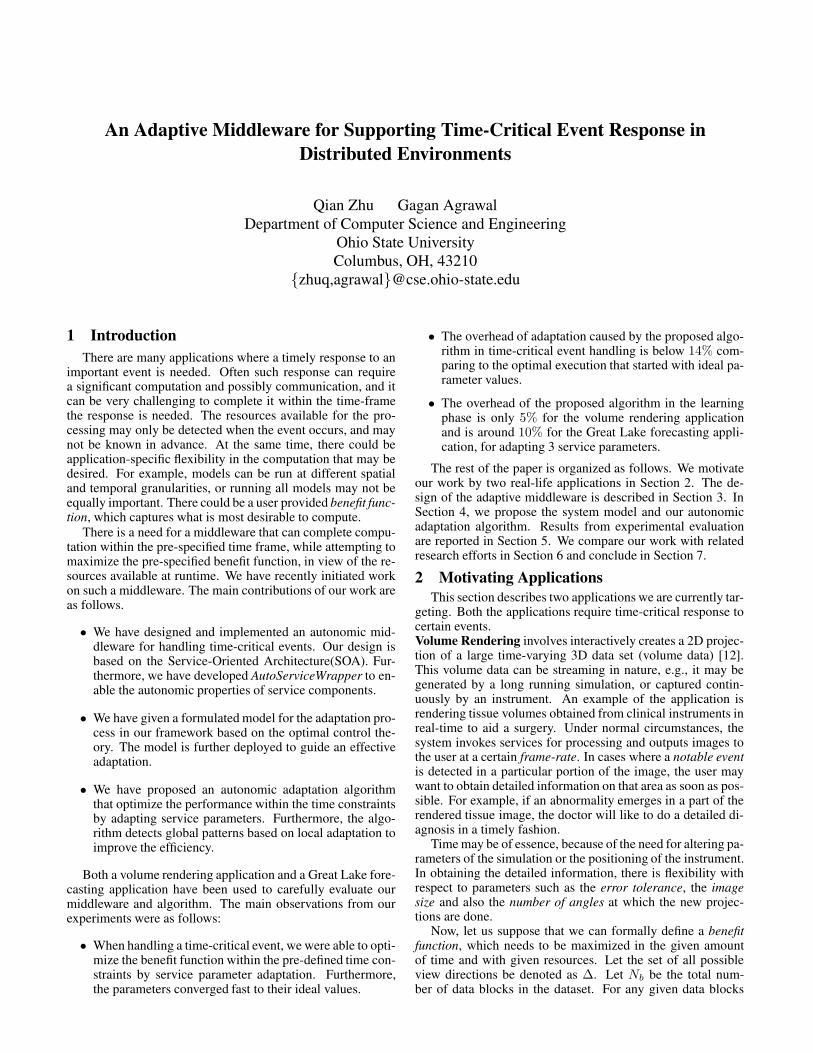
The overall system architecture is illustrated in Figure 1.An application is implemented as a set of loosely-coupled au-tonomic service components, with possible dependencies be-tween them. Each service component is able to self-describeits interface and self-optimize its contribution to the overallprocessing. One service could invoke another service for cer-tain functionality by communicating through SOAP messages.In the VolumeRendering application from the previoussection, the service for constructing a spatial-temporal treewould invoke a service specified in creating a temporal tree,since each leaf node in the spatial tree presents its temporalinformation as a tree structure.

In order to facilitate the implementation of autonomic prop-erties for service components, our middleware includes a Ser-vice Deployment Module, a Performance Module and a Learn-ing Module. When an application is submitted to the sys-tem with its source code and the configuration file, the Ser-vice Deployment Module first decomposes the task and wrapsit into autonomic service components. This is done by Au-toServiceWrapper, which will be discussed in the followingsubsection. Then, the configurator extracts information suchas dependencies between services and input/output specifica-tions for service communication. The purpose of this moduleis to activate the application processing by executing its auto-nomic service components.

Each service component is programmed with adjustableservice parameters, such that the different choice of param-eters could significantly impact the execution time, processing

2

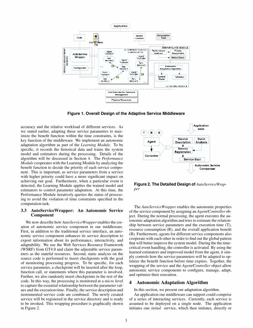
Figure 1. Overall Design of the Adaptive Service Middleware

accuracy and the relative workload of different services. Aswe stated earlier, adapting these service parameters to max-imize the benefit function within the time constraints, is thekey function of the middleware. We implement an autonomicadaptation algorithm as part of the Learning Module. To bespecific, it records the historical data and trains the systemmodel and estimators during the processing. Details of thealgorithm will be discussed in Section 4. The PerformanceModule cooperates with the Learning Module by analyzing thebenefit function to decide the priority of each service compo-nent. This is important, as service parameters from a servicewith higher priority could have a more significant impact onachieving our goal. Furthermore, when a particular event isdetected, the Learning Module applies the trained model andestimators to control parameter adaptation. At this time, thePerformance Module iteratively queries the status of process-ing to avoid the violation of time constraints specified in thecomputation task.

3.3 AutoServiceWrapper: An Autonomic ServiceComponent

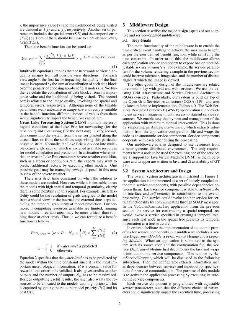
We now describe how AutoServiceWrapper enables the cre-ation of autonomic service component in our middleware.First, in addition to the traditional service interface, an auto-nomic service component enhances its service description toexport information about its performance, interactivity, andadaptability. We use the Web Services Resource Framework(WSRF) from GT4.0 and claim the adjustable service param-eters as the stateful resources. Second, static analysis on thesource code is performed to insert checkpoints with the goalof monitoring processing progress. To be specific, for eachservice parameter, a checkpoint will be inserted after the loop,function call, or statements where this parameter is involved.Further, we also randomly insert checkpoints in the rest of thecode. In this way, the processing is monitored at a micro levelto capture the essential relationship between the parameter val-ues and the execution time. Finally, the service description andinstrumented service code are combined. The newly createdservice will be registered in the service directory and is readyto be invoked. This wrapping procedure is graphically shownin Figure 2.

Figure 2. The Detailed Design of AutoServiceWrap-per

The AutoServiceWrapper enables the autonomic propertiesof the service component by assigning an Agent/Controller ob-ject. During the normal processing, the agent executes the au-tonomic adaptation algorithm and tries to estimate the relation-ship between service parameters and the execution time (T),resource consumption (R), and the overall application benefit(B). Furthermore, agents for different service components alsocooperate with each other in order to find out the global patternthat will better improve the system model. During the the time-critical event handling, the controller is activated. By using thelearned estimators and improved model from the agent, it sim-ply controls how the service parameters will be adapted to op-timize the benefit function before time expires. Together, thewrapping of the service and the Agent/Controller object allowautonomic service components to configure, manage, adapt,and optimize their execution.

4 Autonomic Adaptation AlgorithmIn this section, we present our adaptation algorithm.An application our middleware can support could comprise

of a series of interacting services. Currently, each service isassumed to be deployed on a single node. The applicationinitiates one initial service, which then initiates, directly or

3

indirectly, all other invoked services. The workload of such in-voked service comprises of a series of function calls from theirinvoking service. We assume that we have at least as manynodes available as the services, and a separate node could beused for each service. In the future, we will consider the pos-sibility that each service could be run on parallel platforms.

In such a case, we have three considerations. Obviously, weneed to meet a time constraint, and second, we need to max-imize the benefit function. However, because of the interac-tion between the services, we need to consider another factor,which is the relative workload of each service. The operatingdynamics of a processor P executing one of the services can becaptured by the simple queuing model. At time step k, λ(k)and β(k) denote the average arrival and processing rates asso-ciated with the processor P. The input queue size q(k) indicatesthe current workload on P, which can be calculated as:

q(k) = (λ(k) − β(k)) × Ts (3)

where Ts denotes the sampling period.4.1 Algorithm Overview

The intuition for our approach is as follows. The adapta-tion process in our framework corresponds to a typical optimalcontrol model [10]. The objective of optimal control theoryis to determine the control signals that will cause a process tosatisfy the physical constraints, and at the same time, mini-mize (or maximize) some performance criterion. The input toour middleware is a number of service components with de-pendencies involved. Each of them is programmed with ad-justable service parameters, as we had previously shown in ourexamples. When a particular event occurs, our algorithm con-trols the adaptation of the service parameters so as to optimizethe benefit function, while satisfying the physical constraints,which are the pre-defined time interval and relative workloadof the services. We assume that our processing comprises a se-ries of processing rounds, and values of all service parameterscan be modified between two processing rounds.

Our approach is to first build a model for a particular ap-plication by estimating the effect of service parameters on ex-ecution time, relative workload of different services, and thebenefit function. Then, this model is deployed in the adapta-tion process of the application. In the VolumeRenderingapplication, the model specifies how ErrorTolerance andImageSize would be changed based on their values from theprevious time step and the current action (increase/decreaseand by how much). However, the control problem of adjust-ing service parameters is a high-dimensional continuous-statetask. For example, ErrorTolerance is a real number between0 and 1. Then its control signal could be any real number aslong as the new value remains in the range. It is extremely dif-ficult to build an accurate model from the beginning. We pro-pose an autonomic adaption algorithm that is able to quicklylearn to perform well in the parameter adaption. Furthermore,the adaptation action taken at each service component will beconverted to an effect in the overall system. Such global pat-tern could be the correlation between ErrorTolerance andImageSize in our example. Once it is detected, we couldadapt both parameters in a non-conflicting way.

The algorithm falls into two phases, namely, a normal exe-cution phase and a event handling phase. In the normal exe-cution phase, we locally explore different values of service pa-rameters to estimate the relationship between service parame-ters and execution time, relative workload of different services,

Variable Descriptionx(k) Adjustable service parametersu(k) Increase/Decrease to parametersw(k) Estimated overall response timev(k) Corrective termq(k) Relative Workload

Figure 3. Definitions for the Control Model

and the benefit function. Once an event is detected and needsto be handled with a time constraint, the service parameterswill be adapted using the learnt model.4.2 Detailed Problem Formulation

In order to utilize the optimal control theory to model theadaptation process in our framework, we need to define amodel. We variables we use in our model are listed in Table 3.In the VolumeRendering example, the vector of state vari-ables x(k) could be [ErrorTolerance, ImageSize]T . A pos-sible control signal could be [0.005,−20]T , which increasesErrorTolerance by 0.005 and decreases ImageSize by 20.Given the current values of these two parameters, we can es-timate the overall execution time in the processing round K,which is denoted as w(k) and relative workload q(k). Fur-thermore, the corrective term v(k) may have to be appliedbecause of the possible correlation between ErrorToleranceand ImageSize.State Equation: The system then is described by the lineartime-varying discrete-time state equation:

x(k) = Ax(k − 1) + Bu(k) + v(k) (4)

w(k) = w(k − 1) + f(x(k)) (5)

where k = 1 to kN , representing the N processing rounds, andA and B are matrices with time-varying elements [10]. Theydefine the linear relationship between a state variable x(k) inthe current time step and the value from the previous state aswell as its control signal. w(k) includes the time passed forthe previous k−1 steps and the estimation for the current step.Performance Measure: The objective of the control problemwe are considering is to find the sequence ui,...,uN to maxi-mize the following performance criterion.

J =1

2h(

1

w0 − w(N))3 +

N−1∑

k=1

[1

2s(Ben(x(k))) −

1

2ru2(k)] (6)

We denote w0 to be the pre-defined time constraint. The firstterm here is designed to penalize the measure if the time dead-line is missed. The rest of the expression includes the theweighted benefit function and a term for adaptation overhead.The goal is to maximize the benefit function, while minimiz-ing the overhead of adaptation. Parameters h, s and r can bechosen to give a relative weight to meeting the time constraint,maximizing the benefit, and minimizing the adaptation over-head.Physical Constraints: The formulated system model has thefollowing physical constraints.

C1 : xmin ≤ x(k) ≤ xmax (7)

C2 : q(k) ≤ Q (8)

4

The first constraint ensures that each service parameter varieswithin its own value range. The second constraint implies thatthe relative workload for each service component has to bebelow a certain threshold, as specified in the vector Q. Thisvector is an input to the algorithm.4.3 Algorithm Details

This subsection gives a detailed description of the adapta-tion algorithm.

A challenge in our problem is to build an accurate modelto control the adaptation process in the event handling phase.Specifically, based on the system model discussed previously,we have to decide u(k) given a certain state, the correctiveterm v(k), as well as estimating the relationships between ser-vice parameters and execution time, relative workload, and thebenefit function.Initial Policy: We apply a simple gradient-based method asthe initial control policy. To be specific, the control signal u(k)here is based on the difference of a modified benefit functionvalue between x(k) and x(k − 1). The modified benefit func-tion includes the original benefit function associated with theapplication, and an expression capturing the penalty of miss-ing the time constraint. Given the parameter vector x(k − 1),we have two possibilities. We are likely to miss the time con-straint, in which case, u(k) needs to decrease the penalty asso-ciated with missing the time constraint. Alternatively, may notbe missing the time constraint, and we can focus on increasingthe benefit function. This simple initial policy could be writtenas:

u(k) = u(k − 1) + α 5 B (9)where, α is the learning rate and B is the modified benefitfunction. Furthermore, we ignore v(k) in the initial policy.

The disadvantage of this initial policy is that it could causea large adaptation overhead. This overhead is dependent onthe value of α. A large value would lead to a situation wherethe adaptation is an iteration of increasing the service param-eters excessively and then decreasing them excessively. Avery small value would likely result in a very slow conver-gence of the service parameters. We are also not consider-ing the correlation between the different parameters, or for-mally, the term v(k). For example, if the correlation betweenErrorTolerance and ImageSize is negative, we shouldavoid increasing both the parameters simultaneously.Control Policy: We use a reinforcement learning algorithm,i.e., Q-learning [26]. Given a state variable x(k), an actionu(k) should be taken if it has the highest probability to yieldthe maximum estimated action-value Q(x(k), u(k)). We com-pute Q(x(k), u(k)) based on the value of the performancefunction, as captured in Equation 6. During the normal execu-tion phase, we use Boltzmann strategy [26] in Q-learning andconduct nearly pure exploration. For parameters with discon-tinuous values, the algorithm simply tries each possible valuefor this service parameter and records the choice with maxi-mum benefit. However, for continuous parameters, the searchspace for an action is infinite. We define a density function,π(u(k)|x(k)), to be the policy at time step k and draw N sam-ples from the search pace as possible choices for u(k). Thedensity function specifies the probability of choosing an actionu(k) at the current state x(k). Furthermore, a higher probabil-ity to take the action u(k), the more performance gain it couldgenerate. Now, we define the control policy as follows.{

maxu(k) π(u(k)|x(k)) if x is continuousmaxu(k) TableLookUp(x(k), u(k)) otherwise

We use a kernel function [30] with Θ as the function parame-ters. Q-learning updates Θ until it converges.

Besides deciding the control policy, we further make themodel more effective by taking potential global patterns intoaccount. The micro parameter adjustments cumulatively pro-duce patterns we can notice at the macro level. One possibleglobal pattern to detect is the correlation between service pa-rameters. By end of each processing rounds, agents of differ-ent service components communicate with each other and findout how different service parameters are correlated. Thus, withthe guidance of this relationship, we could ignore the actionsthat will lead to conflicts. We denote the correlation as v(k) inthe system model. The other global aspect relates to the rel-ative workload. It assures a balance in the relative progressof different services. Recall from our middleware design, thePerformance Module assigns priority to each service compo-nent. The service component with more importance should bepreserved to run with a balanced workload. This is presentedby constraint C2. A resource reconfiguration will be activatedif C2 is violated.Estimating Relationships: We now discuss how we imple-ment estimators which are used during the normal execution.Time: T = f(xi) Recall that multiple checkpoints are insertedin each service by the AutoServiceWrapper. During the nor-mal execution phase, the value of a service parameter xi andthe execution time of the block of code between two consecu-tive checkpoints, Cj and Ck , are recorded. Then the relation-ship T

j,ki is regressed using Recursive Least Square (RLS) [1].

At the end of the learning phase, all Tj,ki will be summed up

to generate the relationship between the execution time of theservice, denoted as Ti, and its service parameter xi. We furtherextend this relationship to be between xi and the overall pro-cessing time of the application T , according to the dependen-cies of service components. Therefore, in the event handlingphase, we could estimate the time T at each checkpoint, giventhe current value of xi to see whether the time constraint willbe violated or not. If so, xi should be adapted accordingly.Relative Workload: R = g(Xi) Recall that

q(k) = (λ(k) − β(k)) × Ts

where Ts denotes the sampling period. At each service com-ponent, the relationship between β(k) and xi is regressed. Thealgorithm checks the relative workload vector q(k) to preservea balanced workload on services with high priority. Other-wise, service parameters will be adapted to assure better rela-tive workload.Benefit: B = l(Xi) In some cases, the relationship betweena service parameter and the benefit function can be easily de-termined from the expression of the benefit function. How-ever, in some other cases, it may not be as simple. For ex-ample, BenefitV R is not directly expressed as a function ofErrorTolerance or ImageSize. Instead, the values of bothErrorTolerance and ImageSize could impact the numberof blocks to be rendered, which is the first of part in equa-tion 1. Also, ErrorTolerance could be further decomposedto SE and TE, thus impacting the second part in the equation.We infer such relationships during the execution, by seeinghow changing service parameters impacts the parameters thatappear in the expression for the benefit function.

5 Experimental EvaluationThis section presents results from a number of experiments

we conducted to evaluate the middeware and our autonomic

5

adaptation algorithm. Specifically, we had the following goalsin our experiments:

• Demonstrate that the converge quickly while meeting thetime constraint. Furthermore, the final method we useturns out to be significant more effective than a simpleand intuitive approach, which is the initial policy we haddescribed.

• Demonstrate that the overhead of adaptation is modest.For this, we compared the execution to the case wherewe start knowing the optimal parameter choices at thevery beginning. Our normal execution, on the other hand,needs to find these parameters during the initial phases ofthe execution.

• Demonstrate the overhead caused by learning is verysmall.

5.1 Experiment DesignAll our experiments were conducted in two Linux clusters,

each of which consists of 64 computing nodes. Every node has2 Opteron 250 (2.4GHz) processors with 8GB of main mem-ory and 500GB local disk space, interconnected with switched1 Gb/s Ethernet.

The experiments we report were conducted using two ap-plications, which we had described in Section 2. The first ap-plication is VolumeRendering. The procedure includes apreprocessing stage and a rendering stage, for which we cre-ated six services. Once the preprocessing is done, an imagewill be rendered for each time step. An interesting event wasdetected after certain time steps. Then, the detailed informa-tion would be generated in the particular area of the imagewhere the event occurred. The time-varying data we used isa brick-of-byte (BOB) data set from Lawrence Livermore Na-tional Laboratory [2]. The details of VolumeRenderingapplication are shown in Table 4.

There are three adjustable service parameters in this ap-plication. The wavelet coefficient, denoted as ω, is from theCompression Service. Both error tolerance and image size,denoted as τ and φ, are parameters in the Unit Image Process-ing Service. A large value of wavelet coefficient(ω) increasesthe time of compression and decompression and it varies be-tween 4, 6, 8, 12, 16, and 20. Similarly, a small value of er-ror tolerance(τ ), or a big value of image size(φ) implies morecommunication as well as computation. The range of them is[0, 1] and (0,∞), respectively. The benefit function is definedin equation 1. We found out that a smaller value of τ yieldsmore benefit from BenefitV R. The correlation between φ andBenefitV R is positive. Furthermore, τ impacts BenefitV R

more significantly than φ does.The second application is referred to as POM. The resolution

of the computational grids covering the Lake Erie could be var-ied from 2000m×2000m, 1000m×1000m to 500m×500m.We created three services for POM. It started with the forecast-ing model running on top of the grids with the resolution as2000m× 2000m. Then, we simulated an event occurring in aparticular region of the lake. A finer-resolution grid will be ac-tivated to run the model for meteorological information predic-tions over this area. We list the details of the POM applicationin Table 4.

The tunable parameters in this application are the numberof internal time steps (ti), number of external time steps(te),and grid resolution(θ). They are from POM Model Services

and the Grid Resolution Service, respectively. A large valueof ti or te leads to less execution time for the model. A smallresolution means the calculation has to be carried out in a moreaccurate way, thus resulting in a longer time interval. We haddefined the benefit function in equation 2. Through the ex-periments, we estimated that there is a relationship betweenBenefitPOM and ti and te. Furthermore, the correlation isnegative for te and positive for ti.5.2 Autonomic Adaptation Algorithm for Time Con-

straintOur first experiment demonstrated the benefits associated

with the proposed adaptation algorithm. We demonstrated thefast convergence of the service parameters. Furthermore, thisalgorithm is more effective compared to the adaptation underthe initial policy that is discussed in Section 4.2. Both theVolumeRendering and POM applications were used for thisexperiment.

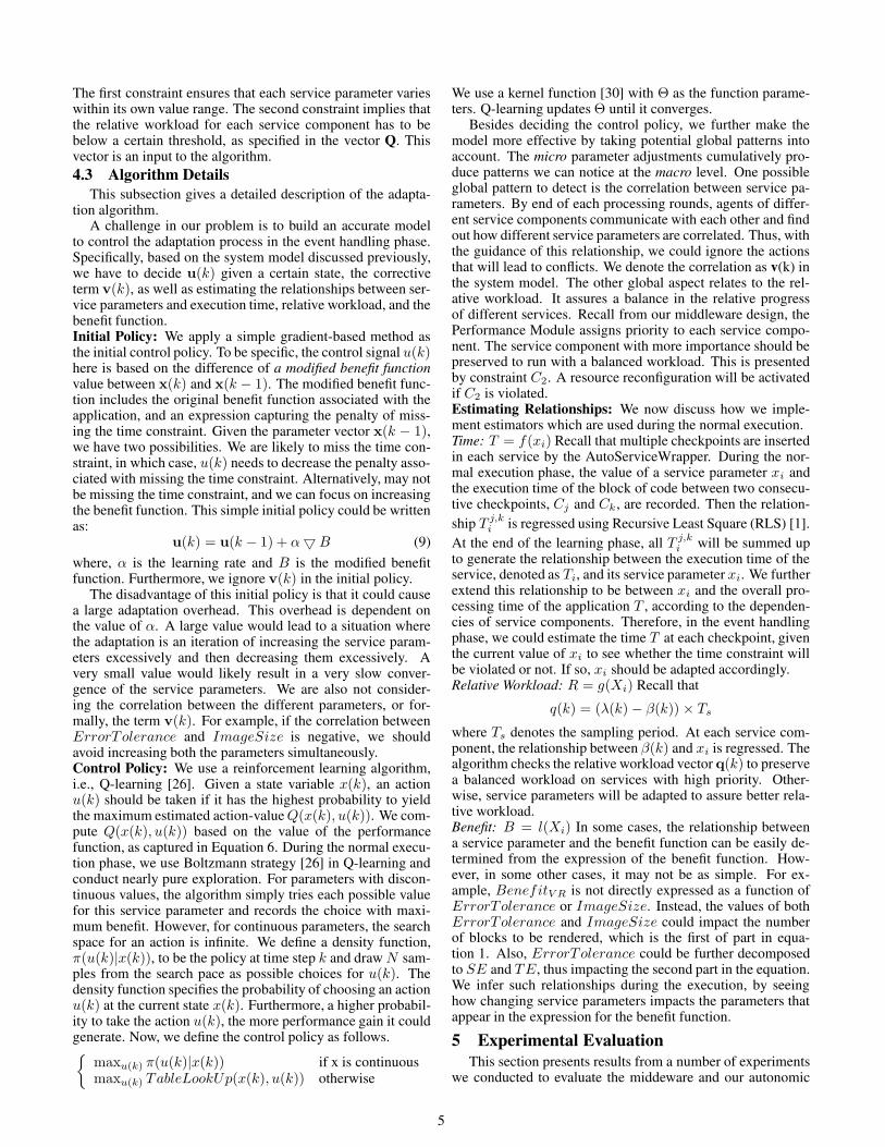
First, we show how the VolumeRendering applicationcould benefit from the algorithm. In a specific computationtask, the user made the following requirements. Within 20minutes, the details of the image should be viewed at least fromview direction of 45◦, 90◦ and 135◦. Furthermore, the resolu-tion of the image should be τ < 0.03 and the ideal image sizefor viewing is 256 × 256. We refer to the case where the ini-tial policy was applied directly to the handling of time-criticalevents as Without Learning. While the case where weapplied the autonomic adaptation algorithm to learn a modelfirst and then used the improved model in the event handlingas With Learning.

The results are as follows. In the With Learning case,all service parameters were able to converge within the timeconstraint with τ = 0.02 and φ = 256× 256. We were able toview the image from 45◦, 75◦, 90◦ and 135◦, each for one ren-dering round. While under Without Learning, althoughfour angels were also generated and τ = 0.027, the image sizewas 232 × 232 which did not satisfy the requirement. This isdue to the inappropriate choices of parameters during the adap-tation under the initial policy that caused an unnecessary over-head. The convergence of the error tolerance is shown in Fig-

0

0.01

0.02

0.03

0.04

0.05

0.06

0.07

0.08

1 2 3 4 5 6 7 8 9 10 11121314151617181920Time Step

Error Tolerance

With Learning

Without Learning

Figure 5. Convergence of Error Tolerance: InitialPolicy vs. Adaptation Algorithm

ure 5. Each checkpoint set in the service code is taken as a timestep where the parameter was adapted, and we have five check-points for each rendering round. As we can see, the adaptationpath of With Learning converged smoothly (decreased

6

App. Services DatasetPreprocessing Rendering

Volume WSTP Tree Construction Service Unit Image Rendering ServiceRendering Temporal Tree Construction Service Decompression Service 6.5GB

Compression Service Image Composition Service (30 time steps)POM Model Service(2-D mode) POM Model Service(3-D mode)

POM Grid Resolution Service Linear Interpolation Service 21.0 GB

Figure 4. Details of the VolumeRendering and POM Applications

monotonically) to an ideal value with τ = 0.02. In compari-son, the adaptation procedure in Without Learning tooksignificant efforts trying to search for an appropriate value forτ . It varied its value in large steps and oscillated in the lastfew steps around 0.027. The reason is that the model whichcontrols adaptation of the parameters specifies the optimal ac-tion to take for the current value, after applying our autonomicadaptation algorithm during the normal execution. The learnedrelationships guaranteed the error tolerance would be adaptedin a way based on information of current resource availabilityand optimal benefit with the minimum effort. Furthermore, thevalue τ converged generated images with higher quality thanrequired, and we saved time for computation of another viewdirection.

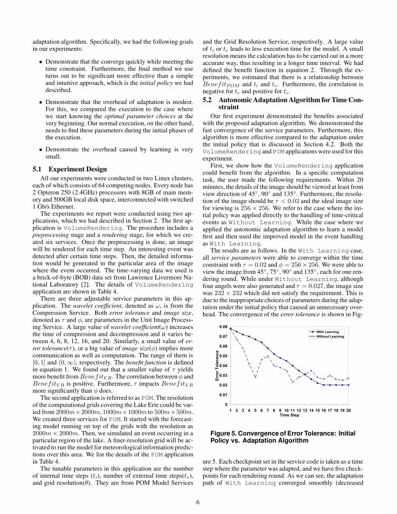
We also demonstrate the results of wavelet coefficient andimage size in Figure 6 and Figure 7, respectively. One factor tonote is that ω stays the same for each rendering round since weonly compressed/decompressed the data block once per round.As a result, we obtained ω = 4 and φ = 256 × 256 in theWithout Learning case and ω = 6 and φ = 232 × 232in the other case. In this application, our proposed algorithmdetected the macro effect as the negative linear correlation be-tween τ and φ. Thus, we tried to increase the value φ if thevalue of τ was decreased.

0

2

4

6

8

10

12

14

16

18

1 2 3 4 5 6 7 8 9 10 11 12 13 14 15 16 17 18 19 20Time Step

Wavelet Coefficients

With Learning

Without Learning

Figure 6. Convergence of Wavelet Coefficient:Initial Policy vs. Adaptation Algorithm

We repeated this experiment with POM application. Wespecified our task to be the following. Given 2 hours, the ap-plication had to forecast the water level of a certain region forthe next two days in the Lake Erie. In order to answer thisquery, the model ran in a 3-d mode with a coarse resolution tobe 2000× 2000 and a finer resolution to be 500 in both WithLearning and Without Learning cases. Furthermore,

0

64

128

192

256

1 2 3 4 5 6 7 8 9 10 11 12 13 14 15 16 17 18 19 20

Time Step

Image Size

With Learning

Without Learning

Figure 7. Convergence of Image Size: Initial Pol-icy vs. Adaptation Algorithm

it was able to forecast more meteorological information forthat particular area, such as water temperature, UM (time av-eraged u velocity at u point), VM (time averaged v velocity atv point) and W (vertical velocity). There are four checkpointsset in the code and POM had four processing rounds, each forone extra output.

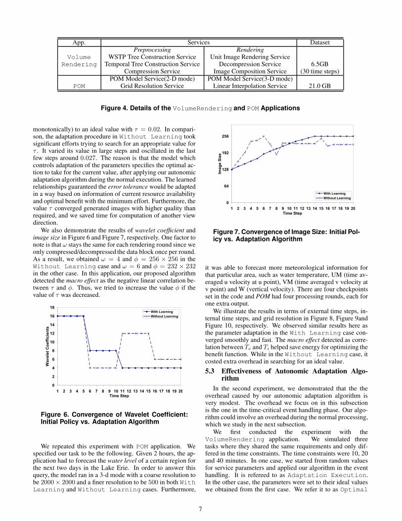
We illustrate the results in terms of external time steps, in-ternal time steps, and grid resolution in Figure 8, Figure 9andFigure 10, respectively. We observed similar results here asthe parameter adaptation in the With Learning case con-verged smoothly and fast. The macro effect detected as corre-lation between Te and Ti helped save energy for optimizing thebenefit function. While in the Without Learning case, itcosted extra overhead in searching for an ideal value.

5.3 Effectiveness of Autonomic Adaptation Algo-rithm

In the second experiment, we demonstrated that the theoverhead caused by our autonomic adaptation algorithm isvery modest. The overhead we focus on in this subsectionis the one in the time-critical event handling phase. Our algo-rithm could involve an overhead during the normal processing,which we study in the next subsection.

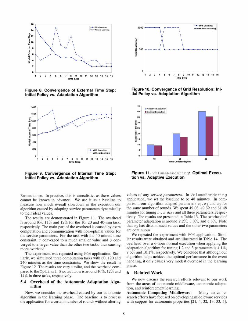
We first conducted the experiment with theVolumeRendering application. We simulated threetasks where they shared the same requirements and only dif-fered in the time constraints. The time constraints were 10, 20and 40 minutes. In one case, we started from random valuesfor service parameters and applied our algorithm in the eventhandling. It is refereed to as Adaptation Execution.In the other case, the parameters were set to their ideal valueswe obtained from the first case. We refer it to as Optimal

7

0

2

4

6

8

10

12

14

16

1 2 3 4 5 6 7 8 9 10 11 12 13 14 15 16

Time Step

Model External Time Step

With Learning

Without Learning

Figure 8. Convergence of External Time Step:Initial Policy vs. Adaptation Algorithm

0

200

400

600

800

1000

1200

1400

1 2 3 4 5 6 7 8 9 10 11 12 13 14 15 16

Time Step

Model Internal Time Step

With Learning

Without Learning

Figure 9. Convergence of Internal Time Step:Initial Policy vs. Adaptation Algorithm

Execution. In practice, this is unrealistic, as these valuescannot be known in advance. We use it as a baseline tomeasure how much overall slowdown in the execution ouralgorithm caused by adapting service parameters dynamicallyto their ideal values.

The results are demonstrated in Figure 11. The overheadis around 9%, 11% and 12% for the 10, 20 and 40-min task,respectively. The main part of the overhead is caused by extracomputation and communication with non-optimal values forthe service parameters. For the task with the 40-minute timeconstraint, τ converged to a much smaller value and φ con-verged to a larger value than the other two tasks, thus causingmore overhead.

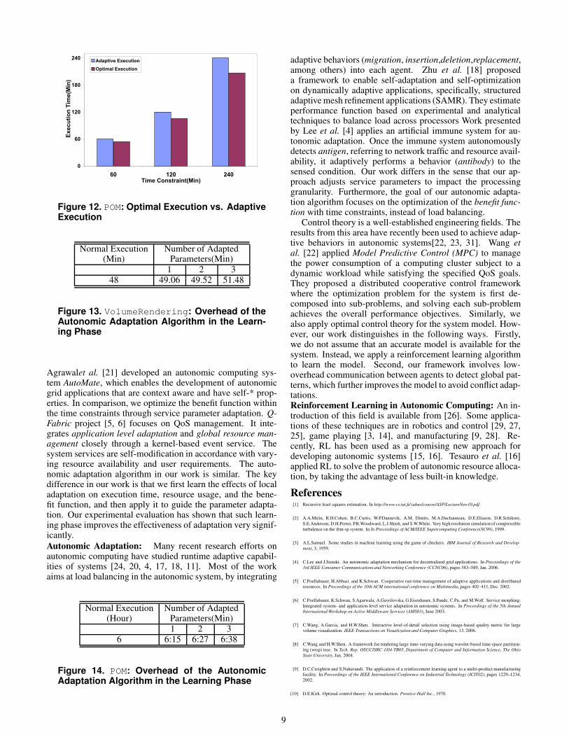
The experiment was repeated using POM application. Sim-ilarly, we simulated three computation tasks with 60, 120 and240 minutes as the time constraints. We show the result inFigure 12. The results are very similar, and the overhead com-pared to the Optimal Execution is around 10%, 12% and14% in three tasks, respectively.

5.4 Overhead of the Autonomic Adaptation Algo-rithm

Now, we consider the overhead caused by our autonomicalgorithm in the learning phase. The baseline is to processthe application for a certain number of rounds without altering

0

500

1000

1 2 3 4 5 6 7 8 9 10 11 12 13 14 15 16

Time Step

Grid Resolution

With Learning

Without Learning

Figure 10. Convergence of Grid Resolution: Ini-tial Policy vs. Adaptation Algorithm

0

5

10

15

20

25

30

35

40

45

10 20 40Time Constaints(Min)

Execution Time (Min)

Adaptive Execution

Optimal Execution

Figure 11. VolumeRendering: Optimal Execu-tion vs. Adaptive Execution

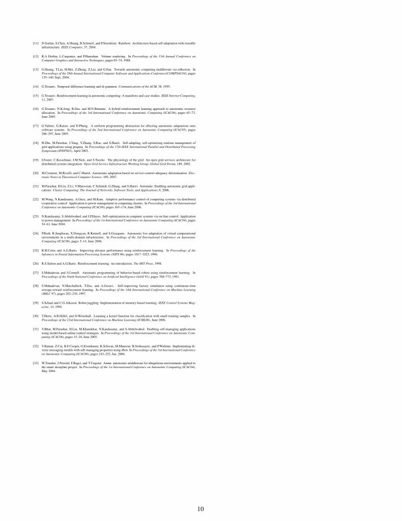
values of any service parameters. In VolumeRenderingapplication, we set the baseline to be 48 minutes. In com-parison, our algorithm adapted parameters x1, x2 and x3 forthe same number of rounds. We spent 49.06, 49.52 and 51.48minutes for tuning x1, x1&x2 and all three parameters, respec-tively. The results are presented in Table 13. The overhead ofparameter adaptation is around 2.2%, 3.0%, and 4.8%. Notethat x2 has discontinued values and the other two parametersare continuous.

We repeated the experiment with POM application. Simi-lar results were obtained and are illustrated in Table 14. Theoverhead over a 6-hour normal execution when applying theadaptation algorithm for tuning 1,2 and 3 parameters is 4.1%,7.5% and 10.1%, respectively. We conclude that although ouralgorithm helps achieve the optimal performance in the eventhandling, it only causes very modest overhead in the learningphase.

6 Related WorkWe now discuss the research efforts relevant to our work

from the areas of autonomic middleware, autonomic adapta-tion, and reinforcement learning.Autonomic Computing Middleware: Many active re-search efforts have focused on developing middleware serviceswith support for autonomic properties [21, 4, 32, 13, 33, 5].

8

0

60

120

180

240

60 120 240Time Constraint(Min)

Execution Time(Min)

Adaptive Execution

Optimal Execution

Figure 12. POM: Optimal Execution vs. AdaptiveExecution

Normal Execution Number of Adapted(Min) Parameters(Min)

1 2 348 49.06 49.52 51.48

Figure 13. VolumeRendering: Overhead of theAutonomic Adaptation Algorithm in the Learn-ing Phase

Agrawalet al. [21] developed an autonomic computing sys-tem AutoMate, which enables the development of autonomicgrid applications that are context aware and have self-* prop-erties. In comparison, we optimize the benefit function withinthe time constraints through service parameter adaptation. Q-Fabric project [5, 6] focuses on QoS management. It inte-grates application level adaptation and global resource man-agement closely through a kernel-based event service. Thesystem services are self-modification in accordance with vary-ing resource availability and user requirements. The auto-nomic adaptation algorithm in our work is similar. The keydifference in our work is that we first learn the effects of localadaptation on execution time, resource usage, and the bene-fit function, and then apply it to guide the parameter adapta-tion. Our experimental evaluation has shown that such learn-ing phase improves the effectiveness of adaptation very signif-icantly.Autonomic Adaptation: Many recent research efforts onautonomic computing have studied runtime adaptive capabil-ities of systems [24, 20, 4, 17, 18, 11]. Most of the workaims at load balancing in the autonomic system, by integrating

Normal Execution Number of Adapted(Hour) Parameters(Min)

1 2 36 6:15 6:27 6:38

Figure 14. POM: Overhead of the AutonomicAdaptation Algorithm in the Learning Phase

adaptive behaviors (migration, insertion,deletion,replacement,among others) into each agent. Zhu et al. [18] proposeda framework to enable self-adaptation and self-optimizationon dynamically adaptive applications, specifically, structuredadaptive mesh refinement applications (SAMR). They estimateperformance function based on experimental and analyticaltechniques to balance load across processors Work presentedby Lee et al. [4] applies an artificial immune system for au-tonomic adaptation. Once the immune system autonomouslydetects antigen, referring to network traffic and resource avail-ability, it adaptively performs a behavior (antibody) to thesensed condition. Our work differs in the sense that our ap-proach adjusts service parameters to impact the processinggranularity. Furthermore, the goal of our autonomic adapta-tion algorithm focuses on the optimization of the benefit func-tion with time constraints, instead of load balancing.

Control theory is a well-established engineering fields. Theresults from this area have recently been used to achieve adap-tive behaviors in autonomic systems[22, 23, 31]. Wang etal. [22] applied Model Predictive Control (MPC) to managethe power consumption of a computing cluster subject to adynamic workload while satisfying the specified QoS goals.They proposed a distributed cooperative control frameworkwhere the optimization problem for the system is first de-composed into sub-problems, and solving each sub-problemachieves the overall performance objectives. Similarly, wealso apply optimal control theory for the system model. How-ever, our work distinguishes in the following ways. Firstly,we do not assume that an accurate model is available for thesystem. Instead, we apply a reinforcement learning algorithmto learn the model. Second, our framework involves low-overhead communication between agents to detect global pat-terns, which further improves the model to avoid conflict adap-tations.Reinforcement Learning in Autonomic Computing: An in-troduction of this field is available from [26]. Some applica-tions of these techniques are in robotics and control [29, 27,25], game playing [3, 14], and manufacturing [9, 28]. Re-cently, RL has been used as a promising new approach fordeveloping autonomic systems [15, 16]. Tesauro et al. [16]applied RL to solve the problem of autonomic resource alloca-tion, by taking the advantage of less built-in knowledge.

References[1] Recursive least squares estimation. In http://www.cs.tut.fi/ tabus/course/ASP/LectureNew10.pdf.

[2] A.A.Mirin, R.H.Cohen, B.C.Curtis, W.P.Dannevik, A.M. Dimits, M.A.Duchauneau, D.E.Eliason, D.R.Schikore,S.E.Anderson, D.H.Porter, P.R.Woodward, L.J.Shieh, and S.W.White. Very high resolution simulation of compressibleturbulence on the ibm-sp system. In In Proceedings of ACM/IEEE Supercomputing Conference(SC99), 1999.

[3] A.L.Samuel. Some studies in machine learning using the game of checkers. IBM Journal of Research and Develop-ment, 3, 1959.

[4] C.Lee and J.Suzuki. An autonomic adaptation mechanism for decentralized grid applications. In Proceedings of the3rd IEEE Consumer Communications and Networking Conference (CCNC06), pages 583–589, Jan. 2006.

[5] C.Poellabauer, H.Abbasi, and K.Schwan. Cooperative run-time management of adaptive applications and distributedresources. In Proceedings of the 10th ACM international conference on Multimedia, pages 402–411, Dec. 2002.

[6] C.Poellabauer, K.Schwan, S.Agarwala, A.Gavrilovska, G.Eisenhauer, S.Pande, C.Pu, and M.Wolf. Service morphing:Integrated system- and application-level service adaptation in autonomic systems. In Proceedings of the 5th AnnualInternational Workshop on Active Middleware Services (AMS03), June 2003.

[7] C.Wang, A.Garcia, and H.W.Shen. Interactive level-of-detail selection using image-based quality metric for largevolume visualization. IEEE Transactions on Visualization and Computer Graphics, 13, 2006.

[8] C.Wang and H.W.Shen. A framework for rendering large time-varying data using wavelet-based time-space partition-ing (wtsp) tree. In Tech. Rep. OSUCISRC-1/04-TR05, Department of Computer and Information Science, The OhioState University, Jan. 2004.

[9] D.C.Creighton and S.Nahavandi. The application of a reinforcement learning agent to a multi-product manufacturingfacility. In Proceedings of the IEEE International Conference on Industrial Technology (ICIT02), pages 1229–1234,2002.

[10] D.E.Kirk. Optimal control theory: An introduction. Prentice-Hall Inc., 1970.

9

[11] D.Garlan, S.Chen, A.Huang, B.Schmerl, and P.Steenkiste. Rainbow: Architecture-based self-adaptation with reusableinfrastructure. IEEE Computer, 37, 2004.

[12] R.A Drebin, L.Carpenter, and P.Hanrahan. Volume rendering. In Proceedings of the 15th Annual Conference onComputer Graphics and Interactive Techniques, pages 65–74, 1988.

[13] G.Huang, T.Liu, H.Mei, Z.Zheng, Z.Liu, and G.Fan. Towards autonomic computing middleware via reflection. InProceedings of the 28th Annual International Computer Software and Applications Conference(COMPSAC04), pages135–140, Sept. 2004.

[14] G.Tesauro. Temporal difference learning and td-gammon. Communications of the ACM, 38, 1995.

[15] G.Tesauro. Reinforcement learning in autonomic computing: A manifesto and case studies. IEEE Internet Computing,11, 2007.

[16] G.Tesauro, N.K.Jong, R.Das, and M.N.Bennani. A hybrid reinforcement learning approach to autonomic resourceallocation. In Proceedings of the 3rd International Conference on Autonomic Computing (ICAC06), pages 65–73,June 2005.

[17] G.Valetto, G.Kaiser, and D.Phung. A uniform programming abstraction for effecting autonomic adaptations ontosoftware systems. In Proceedings of the 2nd International Conference on Autonomic Computing (ICAC05), pages286–297, June 2005.

[18] H.Zhu, M.Parashar, J.Yang, Y.Zhang, S.Rao, and S.Hariri. Self-adapting, self-optimizing runtime management ofgrid applications using pragma. In Proceedings of the 17th IEEE International Parallel and Distributed ProcessingSymposium (IPDPS03), April 2003.

[19] I.Foster, C.Kesselman, J.M.Nick, and S.Tuecke. The physiology of the grid: An open grid services architecure fordistributed systems integration. Open Grid Service Infrastructure Working Group, Global Grid Forum, 189, 2002.

[20] M.Cremene, M.Riveill, and C.Martel. Autonomic adaptation based on service-context adequacy determination. Elec-tronic Notes in Theoretical Computer Science, 189, 2007.

[21] M.Parashar, H.Liu, Z.Li, V.Matossian, C.Schmidt, G.Zhang, and S.Hariri. Automate: Enabling autonomic grid appli-cations. Cluster Computing: The Journal of Networks, Software Tools, and Applications, 9, 2006.

[22] M.Wang, N.Kandasamy, A.Guez, and M.Kam. Adaptive performance control of computing systems via distributedcooperative control: Application to power management in computing clusters. In Proceedings of the 3rd InternationalConference on Autonomic Computing (ICAC06), pages 165–174, June 2006.

[23] N.Kandasamy, S.Abdelwahed, and J.P.Hayes. Self-optimization in computer systems via on-line control: Applicationto power management. In Proceedings of the 1st International Conference on Autonomic Computing (ICAC04), pages54–61, June 2004.

[24] P.Ruth, R.Junghwan, X.Dongyan, R.Kennell, and S.Goasguen. Autonomic live adaptation of virtual computationalenvironments in a multi-domain infrastructure. In Proceedings of the 3rd International Conference on AutonomicComputing (ICAC06), pages 5–14, June 2006.

[25] R.H.Crites and A.G.Barto. Improving elevator performance using reinforcement learning. In Proceedings of theAdvances in Neural Information Processing Systems (NIPS 96), pages 1017–1023, 1996.

[26] R.S.Sutton and A.G.Barto. Reinforcement learning: An introduction. The MIT Press, 1998.

[27] S.Mahadevan and J.Connell. Automatic programming of behavior-based robots using reinforcement learning. InProceedings of the Ninth National Conference on Artificial Intelligence (AAAI 91), pages 768–773, 1991.

[28] S.Mahadevan, N.Marchalleck, T.Das, and A.Gosavi. Self-improving factory simulation using continuous-timeaverage-reward reinforcement learning. In Proceedings of the 14th International Conference on Machine Learning(IMLC 97), pages 202–210, 1997.

[29] S.Schaal and C.G.Atkeson. Robot juggling: Implementation of memory-based learning. IEEE Control Systems Mag-azine, 14, 1994.

[30] T.Hertz, A.B.Hillel, and D.Weinshall. Learning a kernel function for classification with small training samples. InProceedings of the 23rd International Conference on Machine Learning (ICML06), June 2006.

[31] V.Bhat, M.Parashar, H.Liu, M.Khandekar, N.Kandasamy, and S.Abdelwahed. Enabling self-managing applicationsusing model-based online control strategies. In Proceedings of the 3rd International Conference on Autonomic Com-puting (ICAC06), pages 15–24, June 2005.

[32] V.Kumar, Z.Cai, B.F.Cooper, G.Eisenhauer, K.Schwan, M.Mansour, B.Seshasayee, and P.Widener. Implementing di-verse messaging models with self-managing properties using iflow. In Proceedings of the 3rd InternationalConferenceon Autonomic Computing (ICAC06), pages 243–252, Jan. 2006.

[33] W.Trumler, J.Petzold, F.Bagci, and T.Ungerer. Amun autonomic middleware for ubiquitious environments applied tothe smart doorplate project. In Proceedings of the 1st International Conference on Autonomic Computing (ICAC04),May 2004.

10