Algorithms Book

CS 473g Algorithms¬

Sariel Har-Peled

December 10, 2007

This work is licensed under the Creative Commons Attribution-Noncommercial 3.0 License. To view a copy ofthis license, visit http://creativecommons.org/licenses/by-nc/3.0/ or send a letter to Creative Commons,171 Second Street, Suite 300, San Francisco, California, 94105, USA.

http://creativecommons.org/licenses/by-nc/3.0/

2

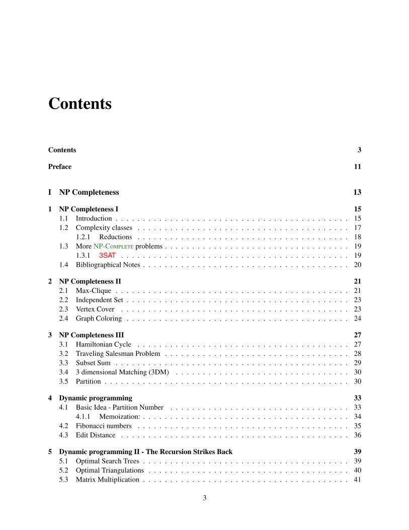
Contents

Contents 3

Preface 11

I NP Completeness 13

1 NP Completeness I 151.1 Introduction . . . . . . . . . . . . . . . . . . . . . . . . . . . . . . . . . . . . . . . . . . . 151.2 Complexity classes . . . . . . . . . . . . . . . . . . . . . . . . . . . . . . . . . . . . . . . 17

1.2.1 Reductions . . . . . . . . . . . . . . . . . . . . . . . . . . . . . . . . . . . . . . . 181.3 More NP-C problems . . . . . . . . . . . . . . . . . . . . . . . . . . . . . . . . . . 19

1.3.1 3SAT . . . . . . . . . . . . . . . . . . . . . . . . . . . . . . . . . . . . . . . . . . 191.4 Bibliographical Notes . . . . . . . . . . . . . . . . . . . . . . . . . . . . . . . . . . . . . . 20

2 NP Completeness II 212.1 Max-Clique . . . . . . . . . . . . . . . . . . . . . . . . . . . . . . . . . . . . . . . . . . . 212.2 Independent Set . . . . . . . . . . . . . . . . . . . . . . . . . . . . . . . . . . . . . . . . . 232.3 Vertex Cover . . . . . . . . . . . . . . . . . . . . . . . . . . . . . . . . . . . . . . . . . . 232.4 Graph Coloring . . . . . . . . . . . . . . . . . . . . . . . . . . . . . . . . . . . . . . . . . 24

3 NP Completeness III 273.1 Hamiltonian Cycle . . . . . . . . . . . . . . . . . . . . . . . . . . . . . . . . . . . . . . . 273.2 Traveling Salesman Problem . . . . . . . . . . . . . . . . . . . . . . . . . . . . . . . . . . 283.3 Subset Sum . . . . . . . . . . . . . . . . . . . . . . . . . . . . . . . . . . . . . . . . . . . 293.4 3 dimensional Matching (3DM) . . . . . . . . . . . . . . . . . . . . . . . . . . . . . . . . 303.5 Partition . . . . . . . . . . . . . . . . . . . . . . . . . . . . . . . . . . . . . . . . . . . . . 30

4 Dynamic programming 334.1 Basic Idea - Partition Number . . . . . . . . . . . . . . . . . . . . . . . . . . . . . . . . . 33

4.1.1 Memoization: . . . . . . . . . . . . . . . . . . . . . . . . . . . . . . . . . . . . . . 344.2 Fibonacci numbers . . . . . . . . . . . . . . . . . . . . . . . . . . . . . . . . . . . . . . . 354.3 Edit Distance . . . . . . . . . . . . . . . . . . . . . . . . . . . . . . . . . . . . . . . . . . 36

5 Dynamic programming II - The Recursion Strikes Back 395.1 Optimal Search Trees . . . . . . . . . . . . . . . . . . . . . . . . . . . . . . . . . . . . . . 395.2 Optimal Triangulations . . . . . . . . . . . . . . . . . . . . . . . . . . . . . . . . . . . . . 405.3 Matrix Multiplication . . . . . . . . . . . . . . . . . . . . . . . . . . . . . . . . . . . . . . 41

3

5.4 Longest Ascending Subsequence . . . . . . . . . . . . . . . . . . . . . . . . . . . . . . . . 425.5 Pattern Matching . . . . . . . . . . . . . . . . . . . . . . . . . . . . . . . . . . . . . . . . 42

6 Approximation algorithms 456.1 Greedy algorithms and approximation algorithms . . . . . . . . . . . . . . . . . . . . . . . 45

6.1.1 Alternative algorithm – two for the price of one . . . . . . . . . . . . . . . . . . . . 476.2 Traveling Salesman Person . . . . . . . . . . . . . . . . . . . . . . . . . . . . . . . . . . . 47

6.2.1 TSP with the triangle inequality . . . . . . . . . . . . . . . . . . . . . . . . . . . . 486.2.1.1 A 2-approximation . . . . . . . . . . . . . . . . . . . . . . . . . . . . . . 486.2.1.2 A 3/2-approximation to TSP4,-Min . . . . . . . . . . . . . . . . . . . . 49

7 Approximation algorithms II 517.1 Max Exact 3SAT . . . . . . . . . . . . . . . . . . . . . . . . . . . . . . . . . . . . . . . . 517.2 Approximation Algorithms for Set Cover . . . . . . . . . . . . . . . . . . . . . . . . . . . 52

7.2.1 Guarding an Art Gallery . . . . . . . . . . . . . . . . . . . . . . . . . . . . . . . . 527.2.2 Set Cover . . . . . . . . . . . . . . . . . . . . . . . . . . . . . . . . . . . . . . . . 53

7.3 Biographical Notes . . . . . . . . . . . . . . . . . . . . . . . . . . . . . . . . . . . . . . . 54

8 Approximation algorithms III 558.1 Clustering . . . . . . . . . . . . . . . . . . . . . . . . . . . . . . . . . . . . . . . . . . . . 55

8.1.1 The approximation algorithm for k-center clustering . . . . . . . . . . . . . . . . . 568.2 Subset Sum . . . . . . . . . . . . . . . . . . . . . . . . . . . . . . . . . . . . . . . . . . . 58

8.2.1 On the complexity of ε-approximation algorithms . . . . . . . . . . . . . . . . . . . 598.2.2 Approximating subset-sum . . . . . . . . . . . . . . . . . . . . . . . . . . . . . . . 59

8.2.2.1 Bounding the running time of ApproxSubsetSum . . . . . . . . . . . . . 608.2.2.2 The result . . . . . . . . . . . . . . . . . . . . . . . . . . . . . . . . . . 61

8.3 Approximate Bin Packing . . . . . . . . . . . . . . . . . . . . . . . . . . . . . . . . . . . . 618.4 Bibliographical notes . . . . . . . . . . . . . . . . . . . . . . . . . . . . . . . . . . . . . . 62

II Randomized Algorithms 63

9 Randomized Algorithms 659.1 Some Probability . . . . . . . . . . . . . . . . . . . . . . . . . . . . . . . . . . . . . . . . 659.2 Sorting Nuts and Bolts . . . . . . . . . . . . . . . . . . . . . . . . . . . . . . . . . . . . . 66

9.2.1 Running time analysis . . . . . . . . . . . . . . . . . . . . . . . . . . . . . . . . . 669.2.1.1 Alternative incorrect solution . . . . . . . . . . . . . . . . . . . . . . . . 67

9.2.2 What are randomized algorithms? . . . . . . . . . . . . . . . . . . . . . . . . . . . 679.3 Analyzing QuickSort . . . . . . . . . . . . . . . . . . . . . . . . . . . . . . . . . . . . . . 68

10 Randomized Algorithms II 6910.1 QuickSort with High Probability . . . . . . . . . . . . . . . . . . . . . . . . . . . . . . . . 69

10.1.1 Proving that an elements participates in small number of rounds. . . . . . . . . . . . 6910.2 Chernoff inequality . . . . . . . . . . . . . . . . . . . . . . . . . . . . . . . . . . . . . . . 70

10.2.1 Preliminaries . . . . . . . . . . . . . . . . . . . . . . . . . . . . . . . . . . . . . . 7010.2.2 Chernoff inequality . . . . . . . . . . . . . . . . . . . . . . . . . . . . . . . . . . . 71

10.2.2.1 The Chernoff Bound — General Case . . . . . . . . . . . . . . . . . . . . 73

4

11 Min Cut 7511.1 Min Cut . . . . . . . . . . . . . . . . . . . . . . . . . . . . . . . . . . . . . . . . . . . . . 75

11.1.1 Problem Definition . . . . . . . . . . . . . . . . . . . . . . . . . . . . . . . . . . . 7511.1.2 Some Definitions . . . . . . . . . . . . . . . . . . . . . . . . . . . . . . . . . . . . 75

11.2 The Algorithm . . . . . . . . . . . . . . . . . . . . . . . . . . . . . . . . . . . . . . . . . 7611.2.1 Analysis . . . . . . . . . . . . . . . . . . . . . . . . . . . . . . . . . . . . . . . . 77

11.2.1.1 The probability of success. . . . . . . . . . . . . . . . . . . . . . . . . . 7711.2.1.2 Running time analysis. . . . . . . . . . . . . . . . . . . . . . . . . . . . 78

11.3 A faster algorithm . . . . . . . . . . . . . . . . . . . . . . . . . . . . . . . . . . . . . . . . 7911.4 Bibliographical Notes . . . . . . . . . . . . . . . . . . . . . . . . . . . . . . . . . . . . . . 81

III Network Flow 83

12 Network Flow 8512.1 Network Flow . . . . . . . . . . . . . . . . . . . . . . . . . . . . . . . . . . . . . . . . . . 8512.2 Some properties of flows, max flows, and residual networks . . . . . . . . . . . . . . . . . . 8612.3 The Ford-Fulkerson method . . . . . . . . . . . . . . . . . . . . . . . . . . . . . . . . . . 8912.4 On maximum flows . . . . . . . . . . . . . . . . . . . . . . . . . . . . . . . . . . . . . . . 89

13 Network Flow II - The Vengeance 9113.1 Accountability . . . . . . . . . . . . . . . . . . . . . . . . . . . . . . . . . . . . . . . . . . 9113.2 Ford-Fulkerson Method . . . . . . . . . . . . . . . . . . . . . . . . . . . . . . . . . . . . . 9113.3 The Edmonds-Karp algorithm . . . . . . . . . . . . . . . . . . . . . . . . . . . . . . . . . 9213.4 Applications and extensions for Network Flow . . . . . . . . . . . . . . . . . . . . . . . . . 93

13.4.1 Maximum Bipartite Matching . . . . . . . . . . . . . . . . . . . . . . . . . . . . . 9313.4.2 Extension: Multiple Sources and Sinks . . . . . . . . . . . . . . . . . . . . . . . . 94

14 Network Flow III - Applications 9514.1 Edge disjoint paths . . . . . . . . . . . . . . . . . . . . . . . . . . . . . . . . . . . . . . . 95

14.1.1 Edge-disjoint paths in a directed graphs . . . . . . . . . . . . . . . . . . . . . . . . 9514.1.2 Edge-disjoint paths in undirected graphs . . . . . . . . . . . . . . . . . . . . . . . . 96

14.2 Circulations with demands . . . . . . . . . . . . . . . . . . . . . . . . . . . . . . . . . . . 9714.2.1 Circulations with demands . . . . . . . . . . . . . . . . . . . . . . . . . . . . . . . 97

14.2.1.1 The algorithm for computing a circulation . . . . . . . . . . . . . . . . . 9714.3 Circulations with demands and lower bounds . . . . . . . . . . . . . . . . . . . . . . . . . 9814.4 Applications . . . . . . . . . . . . . . . . . . . . . . . . . . . . . . . . . . . . . . . . . . . 99

14.4.1 Survey design . . . . . . . . . . . . . . . . . . . . . . . . . . . . . . . . . . . . . . 99

15 Network Flow IV - Applications II 10115.1 Airline Scheduling . . . . . . . . . . . . . . . . . . . . . . . . . . . . . . . . . . . . . . . 101

15.1.1 Modeling the problem . . . . . . . . . . . . . . . . . . . . . . . . . . . . . . . . . 10215.1.2 Solution . . . . . . . . . . . . . . . . . . . . . . . . . . . . . . . . . . . . . . . . . 102

15.2 Image Segmentation . . . . . . . . . . . . . . . . . . . . . . . . . . . . . . . . . . . . . . 10315.3 Project Selection . . . . . . . . . . . . . . . . . . . . . . . . . . . . . . . . . . . . . . . . 105

15.3.1 The reduction . . . . . . . . . . . . . . . . . . . . . . . . . . . . . . . . . . . . . . 10515.4 Baseball elimination . . . . . . . . . . . . . . . . . . . . . . . . . . . . . . . . . . . . . . 106

15.4.1 Problem definition . . . . . . . . . . . . . . . . . . . . . . . . . . . . . . . . . . . 107

5

15.4.2 Solution . . . . . . . . . . . . . . . . . . . . . . . . . . . . . . . . . . . . . . . . . 10715.4.3 A compact proof of a team being eliminated . . . . . . . . . . . . . . . . . . . . . . 108

IV Min Cost Flow 109

16 Network Flow V - Min-cost flow 11116.1 Minimum Average Cost Cycle . . . . . . . . . . . . . . . . . . . . . . . . . . . . . . . . . 11116.2 Potentials . . . . . . . . . . . . . . . . . . . . . . . . . . . . . . . . . . . . . . . . . . . . 11316.3 Minimum cost flow . . . . . . . . . . . . . . . . . . . . . . . . . . . . . . . . . . . . . . . 11316.4 A Strongly Polynomial Time Algorithm for Min-Cost Flow . . . . . . . . . . . . . . . . . . 11616.5 Analysis of the Algorithm . . . . . . . . . . . . . . . . . . . . . . . . . . . . . . . . . . . 116

16.5.1 Reduced cost induced by a circulation . . . . . . . . . . . . . . . . . . . . . . . . . 11716.5.2 Bounding the number of iterations . . . . . . . . . . . . . . . . . . . . . . . . . . . 118

16.6 Bibliographical Notes . . . . . . . . . . . . . . . . . . . . . . . . . . . . . . . . . . . . . . 119

V Min Cost Flow 121

17 Network Flow VI - Min-Cost Flow Applications 12317.1 Efficient Flow . . . . . . . . . . . . . . . . . . . . . . . . . . . . . . . . . . . . . . . . . . 12317.2 Efficient Flow with Lower Bounds . . . . . . . . . . . . . . . . . . . . . . . . . . . . . . . 12317.3 Shortest Edge-Disjoint Paths . . . . . . . . . . . . . . . . . . . . . . . . . . . . . . . . . . 12417.4 Covering by Cycles . . . . . . . . . . . . . . . . . . . . . . . . . . . . . . . . . . . . . . . 12417.5 Minimum weight bipartite matching . . . . . . . . . . . . . . . . . . . . . . . . . . . . . . 12417.6 The transportation problem . . . . . . . . . . . . . . . . . . . . . . . . . . . . . . . . . . . 125

VI Fast Fourier Transform 127

18 Fast Fourier Transform 12918.1 Introduction . . . . . . . . . . . . . . . . . . . . . . . . . . . . . . . . . . . . . . . . . . . 12918.2 Computing a polynomial quickly on n values . . . . . . . . . . . . . . . . . . . . . . . . . 130

18.2.1 Generating Collapsible Sets . . . . . . . . . . . . . . . . . . . . . . . . . . . . . . 13118.3 Recovering the polynomial . . . . . . . . . . . . . . . . . . . . . . . . . . . . . . . . . . . 13218.4 The Convolution Theorem . . . . . . . . . . . . . . . . . . . . . . . . . . . . . . . . . . . 134

VII Sorting Networks 135

19 Sorting Networks 13719.1 Model of Computation . . . . . . . . . . . . . . . . . . . . . . . . . . . . . . . . . . . . . 13719.2 Sorting with a circuit – a naive solution . . . . . . . . . . . . . . . . . . . . . . . . . . . . 138

19.2.1 Definitions . . . . . . . . . . . . . . . . . . . . . . . . . . . . . . . . . . . . . . . 13819.2.2 Sorting network based on insertion sort . . . . . . . . . . . . . . . . . . . . . . . . 138

19.3 The Zero-One Principle . . . . . . . . . . . . . . . . . . . . . . . . . . . . . . . . . . . . . 13919.4 A bitonic sorting network . . . . . . . . . . . . . . . . . . . . . . . . . . . . . . . . . . . . 140

19.4.1 Merging sequence . . . . . . . . . . . . . . . . . . . . . . . . . . . . . . . . . . . 14119.5 Sorting Network . . . . . . . . . . . . . . . . . . . . . . . . . . . . . . . . . . . . . . . . . 141

6

19.6 Faster sorting networks . . . . . . . . . . . . . . . . . . . . . . . . . . . . . . . . . . . . . 142

VIII Linear Programming 143

20 Linear Programming 14520.1 Introduction and Motivation . . . . . . . . . . . . . . . . . . . . . . . . . . . . . . . . . . 145

20.1.1 History . . . . . . . . . . . . . . . . . . . . . . . . . . . . . . . . . . . . . . . . . 14520.1.2 Network flow via linear programming . . . . . . . . . . . . . . . . . . . . . . . . . 146

20.2 The Simplex Algorithm . . . . . . . . . . . . . . . . . . . . . . . . . . . . . . . . . . . . . 14620.2.1 Linear program where all the variables are positive . . . . . . . . . . . . . . . . . . 14620.2.2 Standard form . . . . . . . . . . . . . . . . . . . . . . . . . . . . . . . . . . . . . . 14620.2.3 Slack Form . . . . . . . . . . . . . . . . . . . . . . . . . . . . . . . . . . . . . . . 14720.2.4 The Simplex algorithm by example . . . . . . . . . . . . . . . . . . . . . . . . . . 148

20.2.4.1 Starting somewhere . . . . . . . . . . . . . . . . . . . . . . . . . . . . . 150

21 Linear Programming II 15321.1 The Simplex Algorithm in Detail . . . . . . . . . . . . . . . . . . . . . . . . . . . . . . . . 15321.2 The SimplexInner Algorithm . . . . . . . . . . . . . . . . . . . . . . . . . . . . . . . . . 153

21.2.1 Degeneracies . . . . . . . . . . . . . . . . . . . . . . . . . . . . . . . . . . . . . . 15421.2.2 Correctness of linear programming . . . . . . . . . . . . . . . . . . . . . . . . . . 15521.2.3 On the ellipsoid method and interior point methods . . . . . . . . . . . . . . . . . . 155

21.3 Duality and Linear Programming . . . . . . . . . . . . . . . . . . . . . . . . . . . . . . . . 15521.3.1 Duality by Example . . . . . . . . . . . . . . . . . . . . . . . . . . . . . . . . . . 15521.3.2 The Dual Problem . . . . . . . . . . . . . . . . . . . . . . . . . . . . . . . . . . . 15621.3.3 The Weak Duality Theorem . . . . . . . . . . . . . . . . . . . . . . . . . . . . . . 156

22 Approximation Algorithms using Linear Programming 15922.1 Weighted vertex cover . . . . . . . . . . . . . . . . . . . . . . . . . . . . . . . . . . . . . 15922.2 Revisiting Set Cover . . . . . . . . . . . . . . . . . . . . . . . . . . . . . . . . . . . . . . 16122.3 Minimizing congestion . . . . . . . . . . . . . . . . . . . . . . . . . . . . . . . . . . . . . 162

IX Approximate Max Cut 165

23 Approximate Max Cut 16723.1 Problem Statement . . . . . . . . . . . . . . . . . . . . . . . . . . . . . . . . . . . . . . . 167

23.1.1 Analysis . . . . . . . . . . . . . . . . . . . . . . . . . . . . . . . . . . . . . . . . 16823.2 Semi-definite programming . . . . . . . . . . . . . . . . . . . . . . . . . . . . . . . . . . . 16923.3 Bibliographical Notes . . . . . . . . . . . . . . . . . . . . . . . . . . . . . . . . . . . . . . 170

X Learning and Linear Separability 171

24 The Preceptron Algorithm 17324.1 The Preceptron algorithm . . . . . . . . . . . . . . . . . . . . . . . . . . . . . . . . . . . 17324.2 Learning A Circle . . . . . . . . . . . . . . . . . . . . . . . . . . . . . . . . . . . . . . . . 17624.3 A Little Bit On VC Dimension . . . . . . . . . . . . . . . . . . . . . . . . . . . . . . . . . 177

24.3.1 Examples . . . . . . . . . . . . . . . . . . . . . . . . . . . . . . . . . . . . . . . . 177

7

XI Compression, Information and Entropy 179

25 Huffman Coding 18125.1 Huffman coding . . . . . . . . . . . . . . . . . . . . . . . . . . . . . . . . . . . . . . . . . 181

25.1.1 What do we get . . . . . . . . . . . . . . . . . . . . . . . . . . . . . . . . . . . . . 18425.1.2 A formula for the average size of a code word . . . . . . . . . . . . . . . . . . . . . 184

26 Entropy, Randomness, and Information 18726.1 Entropy . . . . . . . . . . . . . . . . . . . . . . . . . . . . . . . . . . . . . . . . . . . . . 187

26.1.1 Extracting randomness . . . . . . . . . . . . . . . . . . . . . . . . . . . . . . . . . 189

27 Even more on Entropy, Randomness, and Information 19127.1 Extracting randomness . . . . . . . . . . . . . . . . . . . . . . . . . . . . . . . . . . . . . 191

27.1.1 Enumerating binary strings with j ones . . . . . . . . . . . . . . . . . . . . . . . . 19127.1.2 Extracting randomness . . . . . . . . . . . . . . . . . . . . . . . . . . . . . . . . . 192

27.2 Bibliographical Notes . . . . . . . . . . . . . . . . . . . . . . . . . . . . . . . . . . . . . . 193

28 Shannon’s theorem 19528.1 Coding: Shannon’s Theorem . . . . . . . . . . . . . . . . . . . . . . . . . . . . . . . . . . 19528.2 Proof of Shannon’s theorem . . . . . . . . . . . . . . . . . . . . . . . . . . . . . . . . . . 196

28.2.1 How to encode and decode efficiently . . . . . . . . . . . . . . . . . . . . . . . . . 19628.2.1.1 The scheme . . . . . . . . . . . . . . . . . . . . . . . . . . . . . . . . . 19628.2.1.2 The proof . . . . . . . . . . . . . . . . . . . . . . . . . . . . . . . . . . 196

28.2.2 Lower bound on the message size . . . . . . . . . . . . . . . . . . . . . . . . . . . 20028.3 Bibliographical Notes . . . . . . . . . . . . . . . . . . . . . . . . . . . . . . . . . . . . . . 200

XII Matchings 201

29 Matchings 20329.1 Definitions . . . . . . . . . . . . . . . . . . . . . . . . . . . . . . . . . . . . . . . . . . . . 20329.2 Unweighted matching in a bipartite graph . . . . . . . . . . . . . . . . . . . . . . . . . . . 20329.3 Matchings and Alternating Paths . . . . . . . . . . . . . . . . . . . . . . . . . . . . . . . . 20329.4 Maximum Weight Matchings in A Bipartite Graph . . . . . . . . . . . . . . . . . . . . . . 205

29.4.1 Faster Algorithm . . . . . . . . . . . . . . . . . . . . . . . . . . . . . . . . . . . . 20629.5 The Bellman-Ford Algorithm - A Quick Reminder . . . . . . . . . . . . . . . . . . . . . . 206

30 Matchings II 20730.1 Maximum Size Matching in a Non-Bipartite Graph . . . . . . . . . . . . . . . . . . . . . . 207

30.1.1 Finding an augmenting path . . . . . . . . . . . . . . . . . . . . . . . . . . . . . . 20730.1.2 The algorithm . . . . . . . . . . . . . . . . . . . . . . . . . . . . . . . . . . . . . . 210

30.1.2.1 Running time analysis . . . . . . . . . . . . . . . . . . . . . . . . . . . . 21030.2 Maximum Weight Matching in A Non-Bipartite Graph . . . . . . . . . . . . . . . . . . . . 210

XIII Union Find 213

31 Union Find 21531.1 Union-Find . . . . . . . . . . . . . . . . . . . . . . . . . . . . . . . . . . . . . . . . . . . 215

8

31.1.1 Requirements from the data-structure . . . . . . . . . . . . . . . . . . . . . . . . . 21531.1.2 Amortized analysis . . . . . . . . . . . . . . . . . . . . . . . . . . . . . . . . . . . 21531.1.3 The data-structure . . . . . . . . . . . . . . . . . . . . . . . . . . . . . . . . . . . 215

31.2 Analyzing the Union-Find Data-Structure . . . . . . . . . . . . . . . . . . . . . . . . . . . 217

XIV Exercises 223

32 Exercises - Prerequisites 22532.1 Graph Problems . . . . . . . . . . . . . . . . . . . . . . . . . . . . . . . . . . . . . . . . . 22532.2 Recurrences . . . . . . . . . . . . . . . . . . . . . . . . . . . . . . . . . . . . . . . . . . . 22732.3 Counting . . . . . . . . . . . . . . . . . . . . . . . . . . . . . . . . . . . . . . . . . . . . 22932.4 O notation and friends . . . . . . . . . . . . . . . . . . . . . . . . . . . . . . . . . . . . . 22932.5 Probability . . . . . . . . . . . . . . . . . . . . . . . . . . . . . . . . . . . . . . . . . . . . 23132.6 Basic data-structures and algorithms . . . . . . . . . . . . . . . . . . . . . . . . . . . . . . 23232.7 General proof thingies . . . . . . . . . . . . . . . . . . . . . . . . . . . . . . . . . . . . . 23532.8 Miscellaneous . . . . . . . . . . . . . . . . . . . . . . . . . . . . . . . . . . . . . . . . . . 235

33 Exercises - NP Completeness 23733.1 Equivalence of optimization and decision problems . . . . . . . . . . . . . . . . . . . . . . 23733.2 Showing problems are NP-C . . . . . . . . . . . . . . . . . . . . . . . . . . . . . . 23833.3 Solving special subcases of NP-C problems in polynomial time . . . . . . . . . . . 239

34 Exercises - Network Flow 24934.1 Network Flow . . . . . . . . . . . . . . . . . . . . . . . . . . . . . . . . . . . . . . . . . . 24934.2 Min Cost Flow . . . . . . . . . . . . . . . . . . . . . . . . . . . . . . . . . . . . . . . . . 257

35 Exercises - Miscellaneous 26135.1 Data structures . . . . . . . . . . . . . . . . . . . . . . . . . . . . . . . . . . . . . . . . . 26135.2 Divide and Conqueror . . . . . . . . . . . . . . . . . . . . . . . . . . . . . . . . . . . . . . 26235.3 Fast Fourier Transform . . . . . . . . . . . . . . . . . . . . . . . . . . . . . . . . . . . . . 26235.4 Union-Find . . . . . . . . . . . . . . . . . . . . . . . . . . . . . . . . . . . . . . . . . . . 26235.5 Lower bounds . . . . . . . . . . . . . . . . . . . . . . . . . . . . . . . . . . . . . . . . . . 26535.6 Number theory . . . . . . . . . . . . . . . . . . . . . . . . . . . . . . . . . . . . . . . . . 26535.7 Sorting networks . . . . . . . . . . . . . . . . . . . . . . . . . . . . . . . . . . . . . . . . 26635.8 Max Cut . . . . . . . . . . . . . . . . . . . . . . . . . . . . . . . . . . . . . . . . . . . . . 266

36 Exercises - Approximation Algorithms 26736.1 Greedy algorithms as approximation algorithms . . . . . . . . . . . . . . . . . . . . . . . . 26736.2 Approxiamtion for hard problems . . . . . . . . . . . . . . . . . . . . . . . . . . . . . . . 268

37 Randomized Algorithms 27137.1 Randomized algorithms . . . . . . . . . . . . . . . . . . . . . . . . . . . . . . . . . . . . . 271

38 Exercises - Linear Programming 27538.1 Miscellaneous . . . . . . . . . . . . . . . . . . . . . . . . . . . . . . . . . . . . . . . . . . 27538.2 Tedious . . . . . . . . . . . . . . . . . . . . . . . . . . . . . . . . . . . . . . . . . . . . . 275

9

39 Exercises - Computational Geometry 27939.1 Misc . . . . . . . . . . . . . . . . . . . . . . . . . . . . . . . . . . . . . . . . . . . . . . . 279

40 Exercises - Entropy 281

Bibliography 283

Index 285

10

Preface

This manuscript is a collection of class notes for the (semi-required graduate) course “473G Algorithms”taught in the University of Illinois, Urbana-Champaign, in the spring of 2006 and fall 2007.

There are without doubt errors and mistakes in the text and I would like to know about them. Pleaseemail me about any of them you find.

Class notes for algorithms class are as common as mushrooms after a rain. I have no plan of publishingthem in any form except on the web. In particular, Jeff Erickson has class notes for 473 which are betterwritten and cover some of the topics in this manuscript (but naturally, I prefer my exposition over his).

My reasons in writing the class notes are to (i) avoid the use of a (prohibitly expensive) book in this class,(ii) cover some topics in a way that deviates from the standard exposition, and (iii) have a clear descriptionof the material covered. In particular, as far as I know, no book covers all the topics discussed here. Also,this manuscript is also available (on the web) in more convenient lecture notes form, where every lecturehas its own chapter.

Most of the topics covered are core topics that I believe every graduate student in computer scienceshould know about. This includes NP-Completeness, dynamic programming, approximation algorithms,randomized algorithms and linear programming. Other topics on the other hand are more additional topicswhich are nice to know about. This includes topics like network flow, minimum-cost network flow, andunion-find. Nevertheless, I strongly believe that knowing all these topics is useful for carrying out anyworthwhile research in any subfield of computer science.

Teaching such a class always involve choosing what not to cover. Some other topics that might beworthy of presentation include fast Fourier transform, the Perceptron algorithm, advanced data-structures,computational geometry, etc – the list goes on. Since this course is for general consumption, more theoreticaltopics were left out.

In any case, these class notes should be taken for what they are. A short (and sometime dense) tour ofsome key topics in theoretical computer science. The interested reader should seek other sources to pursuethem further.

Acknowledgements

(No preface is complete without them.) I would like to thank the students in the class for their input, whichhelped in discovering numerous typos and errors in the manuscript.Furthermore, the content was greatlyeffected by numerous insightful discussions with Jeff Erickson, Edgar Ramos and Chandra Chekuri.

Any remaining errors exist therefore only because they failed to find them, and the reader is encouraged to contact them andcomplain about it. Naaa, just kidding.

11

Getting the source for this work

This work was written using LATEX. Figures were drawn using either xfig (older figures) or ipe (newerfigures). You can get the source code of these class notes from http://valis.cs.uiuc.edu/~sariel/teach/05/b/. See below for detailed copyright notice.

In any case, if you are using these class notes and find them useful, it would be nice if you send me anemail.

Copyright

This work is licensed under the Creative Commons Attribution-Noncommercial 3.0 License. To view a copyof this license, visit http://creativecommons.org/licenses/by-nc/3.0/ or send a letter to CreativeCommons, 171 Second Street, Suite 300, San Francisco, California, 94105, USA.

— Sariel Har-PeledDecember 2007, Urbana, IL

12

http://ipe.compgeom.org/

http://valis.cs.uiuc.edu/~sariel/teach/05/b/

http://valis.cs.uiuc.edu/~sariel/teach/05/b/

http://creativecommons.org/licenses/by-nc/3.0/

Part I

NP Completeness

13

Chapter 1

NP Completeness I

"Then you must begin a reading program immediately so that you man understand the crises of our age," Ignatiussaid solemnly. "Begin with the late Romans, including Boethius, of course. Then you should dip rather extensivelyinto early Medieval. You may skip the Renaissance and the Enlightenment. That is mostly dangerous propaganda.Now, that I think about of it, you had better skip the Romantics and the Victorians, too. For the contemporary period,you should study some selected comic books.""You’re fantastic.""I recommend Batman especially, for he tends to transcend the abysmal society in which he’s found himself. Hismorality is rather rigid, also. I rather respect Batman."

– A confederacy of Dunces, John Kennedy Toole

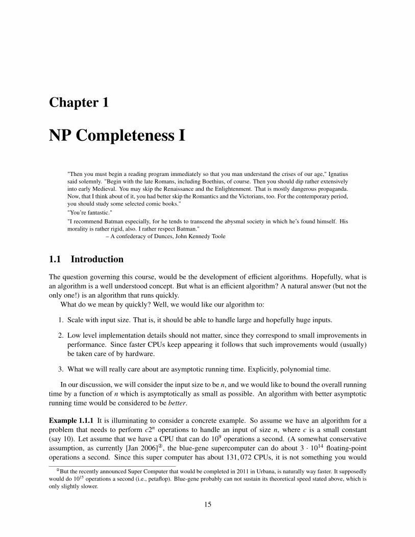
1.1 Introduction

The question governing this course, would be the development of efficient algorithms. Hopefully, what isan algorithm is a well understood concept. But what is an efficient algorithm? A natural answer (but not theonly one!) is an algorithm that runs quickly.

What do we mean by quickly? Well, we would like our algorithm to:

1. Scale with input size. That is, it should be able to handle large and hopefully huge inputs.

2. Low level implementation details should not matter, since they correspond to small improvements inperformance. Since faster CPUs keep appearing it follows that such improvements would (usually)be taken care of by hardware.

3. What we will really care about are asymptotic running time. Explicitly, polynomial time.

In our discussion, we will consider the input size to be n, and we would like to bound the overall runningtime by a function of n which is asymptotically as small as possible. An algorithm with better asymptoticrunning time would be considered to be better.

Example 1.1.1 It is illuminating to consider a concrete example. So assume we have an algorithm for aproblem that needs to perform c2n operations to handle an input of size n, where c is a small constant(say 10). Let assume that we have a CPU that can do 109 operations a second. (A somewhat conservativeassumption, as currently [Jan 2006], the blue-gene supercomputer can do about 3 · 1014 floating-pointoperations a second. Since this super computer has about 131, 072 CPUs, it is not something you would

But the recently announced Super Computer that would be completed in 2011 in Urbana, is naturally way faster. It supposedlywould do 1015 operations a second (i.e., petaflop). Blue-gene probably can not sustain its theoretical speed stated above, which isonly slightly slower.

15

have on your desktop any time soon.) Since 210 ≈ 103, you have that our (cheap) computer can solve in(roughly) 10 seconds a problem of size n = 27.

But what if we increase the problem size to n = 54? This would take our computer about 3 million yearsto solve. (In fact, it is better to just wait for faster computers to show up, and then try to solve the problem.Although there are good reasons to believe that the exponential growth in computer performance we saw inthe last 40 years is about to end. Thus, unless a substantial breakthrough in computing happens, it might bethat solving problems of size, say, n = 100 for this problem would forever be outside our reach.)

The situation dramatically change if we consider an algorithm with running time 10n2. Then, in onesecond our computer can handle input of size n = 104. Problem of size n = 108 can be solved in 10n2/109 =

1017−9 = 108 which is about 3 years of computing (but blue-gene might be able to solve it in less than 20minutes!).

Thus, algorithms that have asymptotically a polynomial running time (i.e., the algorithms running timeis bounded by O(nc) where c is a constant) are able to solve large instances of the input and can solve theproblem even if the problem size increases dramatically.

Can we solve all problems in polynomial time? The answer to this question is unfortunately no. Thereare several synthetic examples of this, but in fact it is believed that a large class of important problems cannot be solved in polynomial time.

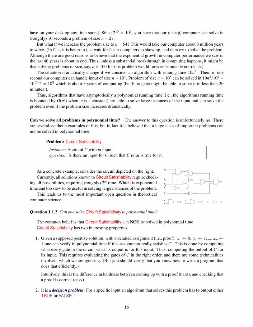
Problem: Circuit Satisfiability

Instance: A circuit C with m inputsQuestion: Is there an input for C such that C returns true for it.

As a concrete example, consider the circuit depicted on the right.Currently, all solutions known to Circuit Satisfiability require check-

ing all possibilities, requiring (roughly) 2m time. Which is exponentialtime and too slow to be useful in solving large instances of the problem.

This leads us to the most important open question in theoreticalcomputer science:

Question 1.1.2 Can one solve Circuit Satisfiability in polynomial time?

The common belief is that Circuit Satisfiability can NOT be solved in polynomial time.Circuit Satisfiability has two interesting properties.

1. Given a supposed positive solution, with a detailed assignment (i.e., proof): x1 ← 0, x2 ← 1, ..., xm ←

1 one can verify in polynomial time if this assignment really satisfies C. This is done by computingwhat every gate in the circuit what its output is for this input. Thus, computing the output of C forits input. This requires evaluating the gates of C in the right order, and there are some technicalitiesinvolved, which we are ignoring. (But you should verify that you know how to write a program thatdoes that efficiently.)

Intuitively, this is the difference in hardness between coming up with a proof (hard), and checking thata proof is correct (easy).

2. It is a decision problem. For a specific input an algorithm that solves this problem has to output eitherTRUE or FALSE.

16

1.2 Complexity classes

Definition 1.2.1 (P: Polynomial time) Let P denote is the class of all decision problems that can be solvedin polynomial time in the size of the input.

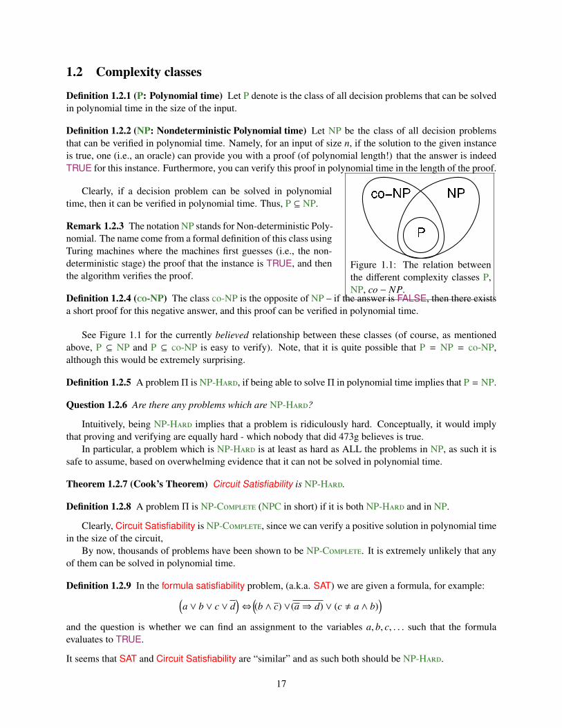
Definition 1.2.2 (NP: Nondeterministic Polynomial time) Let NP be the class of all decision problemsthat can be verified in polynomial time. Namely, for an input of size n, if the solution to the given instanceis true, one (i.e., an oracle) can provide you with a proof (of polynomial length!) that the answer is indeedTRUE for this instance. Furthermore, you can verify this proof in polynomial time in the length of the proof.

Figure 1.1: The relation betweenthe different complexity classes P,NP, co − NP.

Clearly, if a decision problem can be solved in polynomialtime, then it can be verified in polynomial time. Thus, P ⊆ NP.

Remark 1.2.3 The notation NP stands for Non-deterministic Poly-nomial. The name come from a formal definition of this class usingTuring machines where the machines first guesses (i.e., the non-deterministic stage) the proof that the instance is TRUE, and thenthe algorithm verifies the proof.

Definition 1.2.4 (-NP) The class -NP is the opposite of NP – if the answer is FALSE, then there existsa short proof for this negative answer, and this proof can be verified in polynomial time.

See Figure 1.1 for the currently believed relationship between these classes (of course, as mentionedabove, P ⊆ NP and P ⊆ -NP is easy to verify). Note, that it is quite possible that P = NP = -NP,although this would be extremely surprising.

Definition 1.2.5 A problem Π is NP-H, if being able to solve Π in polynomial time implies that P = NP.

Question 1.2.6 Are there any problems which are NP-H?

Intuitively, being NP-H implies that a problem is ridiculously hard. Conceptually, it would implythat proving and verifying are equally hard - which nobody that did 473g believes is true.

In particular, a problem which is NP-H is at least as hard as ALL the problems in NP, as such it issafe to assume, based on overwhelming evidence that it can not be solved in polynomial time.

Theorem 1.2.7 (Cook’s Theorem) Circuit Satisfiability is NP-H.

Definition 1.2.8 A problem Π is NP-C (NPC in short) if it is both NP-H and in NP.

Clearly, Circuit Satisfiability is NP-C, since we can verify a positive solution in polynomial timein the size of the circuit,

By now, thousands of problems have been shown to be NP-C. It is extremely unlikely that anyof them can be solved in polynomial time.

Definition 1.2.9 In the formula satisfiability problem, (a.k.a. SAT) we are given a formula, for example:(a ∨ b ∨ c ∨ d

)⇔

((b ∧ c) ∨(a⇒ d) ∨ (c , a ∧ b)

)and the question is whether we can find an assignment to the variables a, b, c, . . . such that the formulaevaluates to TRUE.

It seems that SAT and Circuit Satisfiability are “similar” and as such both should be NP-H.

17

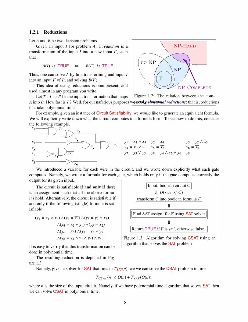
1.2.1 Reductions

NP

co-NP

NP-Hard

P

NP-Complete

Figure 1.2: The relation between the com-plexity classes.

Let A and B be two decision problems.Given an input I for problem A, a reduction is a

transformation of the input I into a new input I′, suchthat

A(I) is TRUE ⇔ B(I′) is TRUE.

Thus, one can solve A by first transforming and input Iinto an input I′ of B, and solving B(I′).

This idea of using reductions is omnipresent, andused almost in any program you write.

Let T : I → I′ be the input transformation that mapsA into B. How fast is T? Well, for our nafarious purposes we need polynomial reductions; that is, reductionsthat take polynomial time.

For example, given an instance of Circuit Satisfiability, we would like to generate an equivalent formula.We will explicitly write down what the circuit computes in a formula form. To see how to do this, considerthe following example.

y1 = x1 ∧ x4 y2 = x4 y3 = y2 ∧ x3y4 = x2 ∨ y1 y5 = x2 y6 = x5y7 = y3 ∨ y5 y8 = y4 ∧ y7 ∧ y6 y8

We introduced a variable for each wire in the circuit, and we wrote down explicitly what each gatecomputes. Namely, we wrote a formula for each gate, which holds only if the gate computes correctly theoutput for its given input.

Input: boolean circuit C

⇓ O(size o f C)

transform C into boolean formula F

⇓

Find SAT assign’ for F using SAT solver

⇓

Return TRUE if F is sat’, otherwise false.

Figure 1.3: Algorithm for solving CSAT using analgorithm that solves the SAT problem

The circuit is satisfiable if and only if thereis an assignment such that all the above formu-las hold. Alternatively, the circuit is satisfiable ifand only if the following (single) formula is sat-isfiable

(y1 = x1 ∧ x4) ∧(y2 = x4) ∧(y3 = y2 ∧ x3)

∧(y4 = x2 ∨ y1) ∧(y5 = x2)

∧(y6 = x5) ∧(y7 = y3 ∨ y5)

∧(y8 = y4 ∧ y7 ∧ y6) ∧ y8.

It is easy to verify that this transformation can bedone in polynomial time.

The resulting reduction is depicted in Fig-ure 1.3.

Namely, given a solver for SAT that runs in TSAT(n), we we can solve the CSAT problem in time

TCS AT (n) ≤ O(n) + TS AT (O(n)),

where n is the size of the input circuit. Namely, if we have polynomial time algorithm that solves SAT thenwe can solve CSAT in polynomial time.

18

Another way of looking at it, is that we believe that solving CSAT requires exponential time; namely,TCSAT(n) ≥ 2n. Which implies by the above reduction that

2n ≤ TCS AT (n) ≤ O(n) + TS AT (O(n)).

Namely, TSAT(n) ≥ 2n/c − O(n), where c is some positive constant. Namely, if we believe that we needexponential time to solve CSAT then we need exponential time to solve SAT.

This implies that if SAT ∈ P then CSAT ∈ P.We just proved that SAT is as hard as CSAT. Clearly, SAT ∈ NP which implies the following theorem.

Theorem 1.2.10 SAT (formula satisfiability) is NP-C.

1.3 More NP-C problems

1.3.1 3SAT

A boolean formula is in conjunctive normal form (CNF) if it is a conjunction (AND) of several clauses,where a clause is the disjunction (or) of several literals, and a literal is either a variable or a negation of avariable. For example, the following is a CNF formula:

clause︷︸︸︷(a ∨ b ∨ c)∧(a ∨ e) ∧ (c ∨ e).

Definition 1.3.1 3CNF formula is a CNF formula with exactly three literals in each clause.

The problem 3SAT is formula satisfiability when the formula is restricted to be a 3CNF formula.

Theorem 1.3.2 3SAT is NP-C.

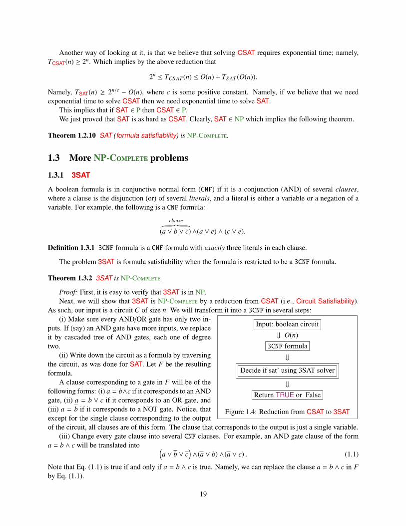
Proof: First, it is easy to verify that 3SAT is in NP.Next, we will show that 3SAT is NP-C by a reduction from CSAT (i.e., Circuit Satisfiability).

As such, our input is a circuit C of size n. We will transform it into a 3CNF in several steps:

Input: boolean circuit

⇓ O(n)

3CNF formula

⇓

Decide if sat’ using 3SAT solver

⇓

Return TRUE or False

Figure 1.4: Reduction from CSAT to 3SAT

(i) Make sure every AND/OR gate has only two in-puts. If (say) an AND gate have more inputs, we replaceit by cascaded tree of AND gates, each one of degreetwo.

(ii) Write down the circuit as a formula by traversingthe circuit, as was done for SAT. Let F be the resultingformula.

A clause corresponding to a gate in F will be of thefollowing forms: (i) a = b∧c if it corresponds to an ANDgate, (ii) a = b ∨ c if it corresponds to an OR gate, and(iii) a = b if it corresponds to a NOT gate. Notice, thatexcept for the single clause corresponding to the outputof the circuit, all clauses are of this form. The clause that corresponds to the output is just a single variable.

(iii) Change every gate clause into several CNF clauses. For example, an AND gate clause of the forma = b ∧ c will be translated into (

a ∨ b ∨ c)∧(a ∨ b) ∧(a ∨ c) . (1.1)

Note that Eq. (1.1) is true if and only if a = b ∧ c is true. Namely, we can replace the clause a = b ∧ c in Fby Eq. (1.1).

19

Similarly, an OR gate clause the form a = b ∨ c in F will be transformed into

(a ∨ b ∨ c) ∧ (a ∨ b) ∧ (a ∨ c).

Finally, a clause a = b, corresponding to a NOT gate, will be transformed into

(a ∨ b) ∧ (a ∨ b).

(iv) Make sure every clause is exactly three literals. Thus, a single variable clause a would be replacedby

(a ∨ x ∨ y) ∧ (a ∨ x ∨ y) ∧ (a ∨ x ∨ y) ∧ (a ∨ x ∨ y),

by introducing two new dummy variables x and y. And a two variable clause a ∨ b would be replaced by

(a ∨ b ∨ y) ∧ (a ∨ b ∨ y),

by introducing the dummy variable y.This completes the reduction, and results in a new 3CNF formula G which is satisfiable if and only if

the original circuit C is satisfiable. The reduction is depicted in Figure 1.3.1. Namely, we generated anequivalent 3CNF to the original circuit. We conclude that if T3SAT(n) is the time required to solve 3SAT then

TCS AT (n) ≤ O(n) + T3S AT (O(n)),

which implies that if we have a polynomial time algorithm for 3SAT, we would solve CSAT is polynomialtime. Namely, 3SAT is NP-C.

1.4 Bibliographical Notes

Cook’s theorem was proved by Stephen Cook (http://en.wikipedia.org/wiki/Stephen_Cook). Itwas proven independently by Leonid Levin (http://en.wikipedia.org/wiki/Leonid_Levin) moreor less in the same time. Thus, this theorem should be referred to as the Cook-Levin theorem.

The standard text on this topic is [GJ90]. Another useful book is [ACG+99], which is a more recent andmore updated, and contain more advanced stuff.

20

http://en.wikipedia.org/wiki/Stephen_Cook

http://en.wikipedia.org/wiki/Leonid_Levin

Chapter 2

NP Completeness II

2.1 Max-Clique

Figure 2.1: A clique of size 4 in-side a graph with 8 vertices.

We remind the reader, that a clique is a complete graph, whereevery pair of vertices are connected by an edge. The MaxCliqueproblem asks what is the largest clique appearing as a subgraph ofG. See Figure 2.1.

Problem: MaxClique

Instance: A graph GQuestion: What is the largest number of nodes in Gforming a complete subgraph?

Note that MaxClique is an optimization problem, since the out-put of the algorithm is a number and not just true/false.

The first natural question, is how to solve MaxClique. A naive algorithm would work by enumeratingall subsets S ⊆ V(G), checking for each such subset S if it induces a clique in G (i.e., all pairs of verticesin S are connected by an edge of G). If so, we know that GS is a clique, where GS denotes the inducedsubgraph on S defined by G; that is, the graph formed by removing all the vertices are not in S from G (inparticular, only edges that have both endpoints in S appear in GS ). Finally, our algorithm would return thelargest S encountered, such that GS is a clique. The running time of this algorithm is O

(2nn2

)as can be

easily verified.

TIPSuggestion 2.1.1 When solving any algorithmic problem, always try first to find a simple (or even naive)solution. You can try optimizing it later, but even a naive solution might give you useful insight into aproblem structure and behavior.

We will prove that MaxClique is NP-H. Before dwelling into that, the simple algorithm we devisedfor MaxClique shade some light on why intuitively it should be NP-H: It does not seem like there is anyway of avoiding the brute force enumeration of all possible subsets of the vertices of G. Thus, a problemis NP-H or NP-C, intuitively, if the only way we know how to solve the problem is to use naivebrute force enumeration of all relevant possibilities.

How to prove that a problem X is NP-H? Proving that a given problem X is NP-H is usually donein two steps. First, we pick a known NP-C problem A. Next, we show how to solve any instance ofA in polynomial time, assuming that we are given a polynomial time algorithm that solves X.

21

Proving that a problem X is NP-C requires the additional burden of showing that is in NP. Note,that only decision problems can be NP-C, but optimization problems can be NP-H; namely, theset of NP-H problems is much bigger than the set of NP-C problems.

Theorem 2.1.2 MaxClique is NP-H.

Proof: We show a reduction from 3SAT. So, consider an input to 3SAT, which is a formula F defined overn variables (and with m clauses).

a b c

a

b

d

b

c

d

a dc

Figure 2.2: The generated graphfor the formula (a ∨ b ∨ c) ∧ (b ∨c ∨ d) ∧ (a ∨ c ∨ d) ∧ (a ∨ b ∨ d).

We build a graph from the formula F by scanning it, as follows:(i) For every literal in the formula we generate a

vertex, and label the vertex with the literal it cor-responds to.

Note, that every clause corresponds to the threesuch vertices.

(ii) We connect two vertices in the graph, if they are:(i) in different clauses, and (ii) they are not anegation of each other.

Let G denote the resulting graph. See Figure 2.2 for a concrete ex-ample. Note, that this reduction can be easily be done in quadratictime in the size of the given formula.

We claim that F is satisfiable iff there exists a clique of size m inG.

⇒ Let x1, . . . , xn be the variables appearing in F, and let v1, . . . , vn ∈ 0, 1 be the satisfying assignmentfor F. Namely, the formula F holds if we set xi = vi, for i = 1, . . . , n.

For every clause C in F there must be at least one literal that evaluates to TRUE. Pick a vertex thatcorresponds to such TRUE value from each clause. Let W be the resulting set of vertices. Clearly, Wforms a clique in G. The set W is of size m, since there are m clauses and each one contribute onevertex to the clique.

⇐ Let U be the set of m vertices which form a clique in G.

We need to translate the clique GU into a satisfying assignment of F.

1. xi ← TRUE if there is a vertex in U labeled with xi.

2. xi ← FALSE if there is a vertex in U labeled with xi.

This is a valid assignment as can be easily verified. Indeed, assume for the sake of contradiction, thatthere is a variable xi such that there are two vertices u, v in U labeled with xi and xi; namely, we aretrying to assign to contradictory values of xi. But then, u and v, by construction will not be connectedin G, and as such GS is not a clique. A contradiction.

Furthermore, this is a satisfying assignment as there is at least one vertex of U in each clause. Imply-ing, that there is a literal evaluating to TRUE in each clause. Namely, F evaluates to TRUE.

Thus, given a polytime (i.e., polynomial time) algorithm for MaxClique, we can solve 3SAT in polytime.We conclude that MaxClique in NP-H.

MaxClique is an optimization problem, but it can be easily restated as a decision problem.

22

(a) (b) (c)

Figure 2.3: (a) A clique in a graph G, (b) the complement graph is formed by all the edges not appearing inG, and (c) the complement graph and the independent set corresponding to the clique in G.

Problem: Clique

Instance: A graph G, integer kQuestion: Is there a clique in G of size k?

Theorem 2.1.3 Clique is NP-C.

Proof: It is NP-H by the previous reduction of Theorem 2.1.2. Thus, we only need to show that it is inNP. This is quite easy. Indeed, given a graph G having n vertices, a parameter k, and a set W of k vertices,verifying that every pair of vertices in W form an edge in G takes O(u + k2), where u is the size of the input(i.e., number of edges + number of vertices). Namely, verifying a positive answer to an instance of Cliquecan be done in polynomial time.

Thus, Clique is NP-C.

2.2 Independent Set

Definition 2.2.1 A set S of nodes in a graph G = (V, E) is an independent set, if no pair of vertices in S areconnected by an edge.

Problem: Independent Set

Instance: A graph G, integer kQuestion: Is there an independent set in G of size k?

Theorem 2.2.2 Independent Set is NP-C.

Proof: We do it by a reduction from Clique. Given G and k, compute the complement graph G where weconnected two vertices u, v in G iff they are independent (i.e., not connected) in G. See Figure 2.3. Clearly,a clique in G corresponds to an independent set in G, and vice versa. Thus, Independent Set is NP-H,and since it is in NP, it is NPC.

2.3 Vertex Cover

Definition 2.3.1 For a graph G, a set of vertices S ⊆ V(G) is a vertex cover if it touches every edge of G.Namely, for every edge uv ∈ E(G) at least one of the endpoints is in S .

23

Problem: Vertex Cover

Instance: A graph G, integer kQuestion: Is there a vertex cover in G of size k?

Lemma 2.3.2 A set S is a vertex cover in G iff V \ S is an independent set in G.

Proof: If S is a vertex cover, then consider two vertices u, v ∈ V \ S . If uv ∈ E(G) then the edge uv is notcovered by S . A contradiction. Thus V \ S is an independent set in G.

Similarly, if V \ S is an independent set in G, then for any edge uv ∈ E(G) it must be that either u or vare not in V \G. Namely, S covers all the edges of G.

Theorem 2.3.3 Vertex Cover is NP-C.

Proof: Vertex Cover is in NP as can be easily verified. To show that it NP-H we will do a reductionfrom Independent Set. So, we are given an instance of Independent Set which is a graph G and parameterk, and we want to know whether there is an independent set in G of size k. By Lemma 2.3.2, G has anindependent set of k iff it has a vertex cover of size n − k. Thus, feeding G and n − k into (the supposedlygiven) black box that can solves vertex cover in polynomial time, we can decide if G has an independent setof size k in polynomial time. Thus Vertex Cover is NP-C.

2.4 Graph Coloring

Definition 2.4.1 A coloring, by c colors, of a graph G = (V, E) is a mapping C : V(G) → 1, 2, . . . , csuch that every vertex is assigned a color (i.e., an integer), such that no two vertices that share an edge areassigned the same color.

Usually, we would like to color a graph with a minimum number of colors. Deciding if a graph can becolored with two colors is equivalent to deciding if a graph bipartite and can be done in linear time usingDFS or BFS.

Coloring is a very useful problem for resource allocation (used in compilers for example) and schedulingtype problems.

Surprisingly, moving from two colors to three colors make the problem much harder.

Problem: 3Colorable

Instance: A graph G.Question: Is there a coloring of G using three colors?

Theorem 2.4.2 3Colorable is NP-C.

Proof: Clearly, 3Colorable is in NP.We prove that it is NP-C by a reduction from 3SAT. Let F be the given 3SAT instance. The

basic idea of the proof is to use gadgets to transform the formula into a graph. Intuitively, a gadget is a smallcomponent that corresponds to some feature of the input.

X

T F

The first gadget will be the color generating gadget, which is formed by three specialvertices connected to each other, where the vertices are denoted by X, F and T , respec-tively. We will consider the color used to color T to correspond to the TRUE value, andthe color of the F to correspond to the FALSE value.

If you do not know the algorithm for this, please read about it to fill the gap in your knowledge.

24

X

a a

For every variable a inF , we will generate a variable gadget, which is (again) a triangleincluding two new vertices, denoted by a and a, and the third vertex is the auxiliary vertexX from the color generating gadget. Note, that in a valid 3-coloring of the resulting grapheither a would be colored by T (i.e., it would be assigned the same color as the color as thevertex T ) and a would be colored by F, or the other way around. Thus, a valid coloring could be interpretedas assigning TRUE or FALSE value to each variable y, by just inspecting the color used for coloring thevertex y.

a

b

c

T

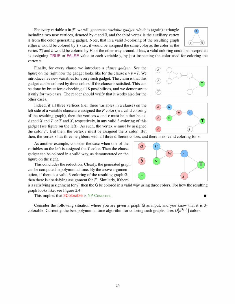
Finally, for every clause we introduce a clause gadget. See thefigure on the right how the gadget looks like for the clause a∨b∨c. Weintroduce five new variables for every such gadget. The claim is that thisgadget can be colored by three colors iff the clause is satisfied. This canbe done by brute force checking all 8 possibilities, and we demonstrateit only for two cases. The reader should verify that it works also for theother cases.

a

b

c

u

Tv

w r

s

Indeed, if all three vertices (i.e., three variables in a clause) on theleft side of a variable clause are assigned the F color (in a valid coloringof the resulting graph), then the vertices u and v must be either be as-signed X and T or T and X, respectively, in any valid 3-coloring of thisgadget (see figure on the left). As such, the vertex w must be assignedthe color F. But then, the vertex r must be assigned the X color. Butthen, the vertex s has three neighbors with all three different colors, and there is no valid coloring for s.

a

b

c

u

Tv

w r

s

As another example, consider the case when one of thevariables on the left is assigned the T color. Then the clausegadget can be colored in a valid way, as demonstrated on thefigure on the right.

This concludes the reduction. Clearly, the generated graphcan be computed in polynomial time. By the above argumen-tation, if there is a valid 3-coloring of the resulting graph G,then there is a satisfying assignment forF . Similarly, if thereis a satisfying assignment forF then the G be colored in a valid way using three colors. For how the resultinggraph looks like, see Figure 2.4.

This implies that 3Colorable is NP-C. ‘

Consider the following situation where you are given a graph G as input, and you know that it is 3-colorable. Currently, the best polynomial time algorithm for coloring such graphs, uses O

(n3/14

)colors.

25

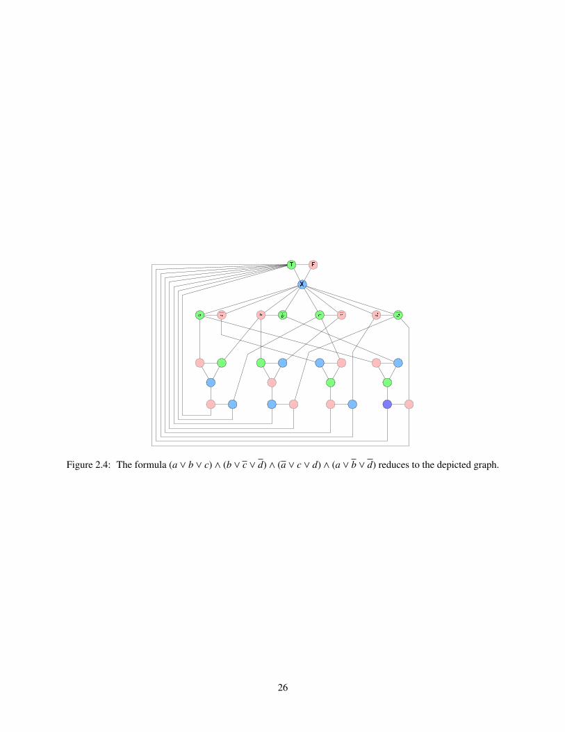
Figure 2.4: The formula (a ∨ b ∨ c) ∧ (b ∨ c ∨ d) ∧ (a ∨ c ∨ d) ∧ (a ∨ b ∨ d) reduces to the depicted graph.

26

Chapter 3

NP Completeness III

3.1 Hamiltonian Cycle

Definition 3.1.1 A Hamiltonian cycle is a cycle in the graph that visits very vertex exactly once.

Definition 3.1.2 An Eulerian cycle is a cycle in a graph that uses every edge exactly once.

Finding Eulerian cycle can be done in linear time. Surprisingly, finding a Hamiltonian cycle is muchharder.

Problem: Hamiltonian Cycle

Instance: A graph G.Question: Is there a Hamiltonian cycle in G?

Theorem 3.1.3 Hamiltonian Cycle is NP-C.

Proof: Hamiltonian Cycle is clearly in NP.

a

b

c

d

e

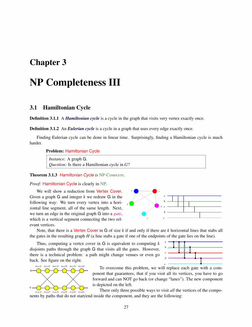
We will show a reduction from Vertex Cover.Given a graph G and integer k we redraw G in thefollowing way: We turn every vertex into a hori-zontal line segment, all of the same length. Next,we turn an edge in the original graph G into a gate,which is a vertical segment connecting the two rel-evant vertices.

Note, that there is a Vertex Cover in G of size k if and only if there are k horizontal lines that stabs allthe gates in the resulting graph H (a line stabs a gate if one of the endpoints of the gate lies on the line).

a

b

c

d

e

Thus, computing a vertex cover in G is equivalent to computing kdisjoints paths through the graph G that visits all the gates. However,there is a technical problem: a path might change venues or even goback. See figure on the right.

(u,v,1) (u,v,6)(u,v,2) (u,v,3) (u,v,4) (u,v,5)

(v,u,1) (v,u,2) (v,u,3) (v,u,4) (v,u,5) (v,u,6)

v

uTo overcome this problem, we will replace each gate with a com-

ponent that guarantees, that if you visit all its vertices, you have to goforward and can NOT go back (or change “lanes”). The new componentis depicted on the left.

There only three possible ways to visit all the vertices of the compo-nents by paths that do not start/end inside the component, and they are the following:

27

The proof that this is the only three possibilities is by brute force.Depicted on the right is one impossible path, that tries to backtrack byentering on the top and leaving on the bottom. Observe, that there arevertices left unvisited. Which means that not all the vertices in the graphare going to be visited, because we add the constraint, that the pathsstart/end outside the gate-component (this condition would be enforced naturally by our final construction).

The resulting graph H1 for the example graph we started with is de-picted on the right. There exists a Vertex Cover in the original graph iffthere exists k paths that start on the left side and end on the right side, inthis weird graph. And these k paths visits all the vertices.

a

b

c

d

e

a

b

c

e

d

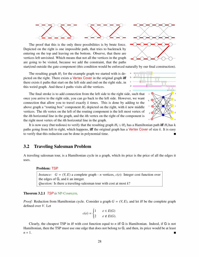
The final stroke is to add connection from the left side to the right side, such thatonce you arrive to the right side, you can go back to the left side. However, we wantconnection that allow you to travel exactly k times. This is done by adding to theabove graph a “routing box” component H2 depicted on the right, with k new middlevertices. The ith vertex on the left of the routing component is the left most vertex ofthe ith horizontal line in the graph, and the ith vertex on the right of the component isthe right most vertex of the ith horizontal line in the graph.

It is now easy (but tedious) to verify that the resulting graph H1 ∪H2 has a Hamiltonian path iff H1has kpaths going from left to right, which happens, iff the original graph has a Vertex Cover of size k. It is easyto verify that this reduction can be done in polynomial time.

3.2 Traveling Salesman Problem

A traveling salesman tour, is a Hamiltonian cycle in a graph, which its price is the price of all the edges ituses.

Problem: TSP

Instance: G = (V, E) a complete graph - n vertices, c(e): Integer cost function overthe edges of G, and k an integer.Question: Is there a traveling-salesman tour with cost at most k?

Theorem 3.2.1 TSP is NP-C.

Proof: Reduction from Hamiltonian cycle. Consider a graph G = (V, E), and let H be the complete graphdefined over V . Let

c(e) =

1 e ∈ E(G)2 e < E(G).

Clearly, the cheapest TSP in H with cost function equal to n iff G is Hamiltonian. Indeed, if G is notHamiltonian, then the TSP must use one edge that does not belong to G, and then, its price would be at leastn + 1.

28

3.3 Subset Sum

We would like to prove that the following problem, Subset Sum is NPC.

Problem: Subset Sum

Instance: S - set of positive integers,t: - an integer number (Target)Question: Is there a subset X ⊆ S such that

∑x∈X x = t?

How does one prove that a problem is NP-C? First, one has to choose an appropriate NPC toreduce from. In this case, we will use 3SAT. Namely, we are given a 3CNF formula with n variables andm clauses. The second stage, is to “play” with the problem and understand what kind of constraints can beencoded in an instance of a given problem and understand the general structure of the problem.

The first observation is that we can use very long numbers as input to Subset Sum. The numbers canbe of polynomial length in the size of the input 3SAT formula F.

The second observation is that in fact, instead of thinking about Subset Sum as adding numbers, we canthink about it as a problem where we are given vectors with k components each, and the sum of the vectors(coordinate by coordinate, must match. For example, the input might be the vectors (1, 2), (3, 4), (5, 6) andthe target vector might be (6, 8). Clearly, (1, 2) + (5, 6) give the required target vector. Lets refer to this newproblem as Vec Subset Sum.

Problem: Vec Subset Sum

Instance: S - set of n vectors of dimension k, each vector has non-negative numbersfor its coordinates, and a target vector −→t .Question: Is there a subset X ⊆ S such that

∑−→x ∈X−→x = −→t ?

Given an instance of Vec Subset Sum, we can covert it into an instance of Subset Sum as follows:We compute the largest number in the given instance, multiply it by n2 · k · 100, and compute how manydigits are required to write this number down. Let U be this number of digits. Now, we take every vector inthe given instance and we write it down using U digits, padding it with zeroes as necessary. Clearly, eachvector is now converted into a huge integer number. The property is now that a sub of numbers in a specificcolumn of the given instance can not spill into digits allocated for a different column since there are enoughzeroes separating the digits corresponding to two different columns.

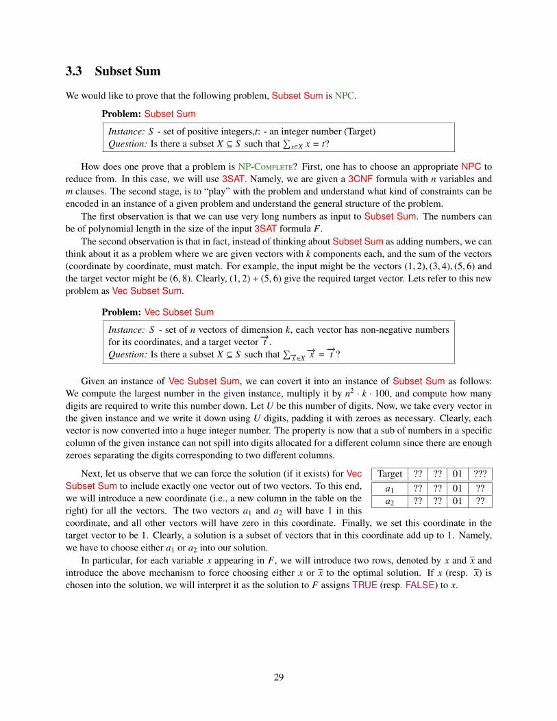
Target ?? ?? 01 ???a1 ?? ?? 01 ??a2 ?? ?? 01 ??

Next, let us observe that we can force the solution (if it exists) for VecSubset Sum to include exactly one vector out of two vectors. To this end,we will introduce a new coordinate (i.e., a new column in the table on theright) for all the vectors. The two vectors a1 and a2 will have 1 in thiscoordinate, and all other vectors will have zero in this coordinate. Finally, we set this coordinate in thetarget vector to be 1. Clearly, a solution is a subset of vectors that in this coordinate add up to 1. Namely,we have to choose either a1 or a2 into our solution.

In particular, for each variable x appearing in F, we will introduce two rows, denoted by x and x andintroduce the above mechanism to force choosing either x or x to the optimal solution. If x (resp. x) ischosen into the solution, we will interpret it as the solution to F assigns TRUE (resp. FALSE) to x.

29

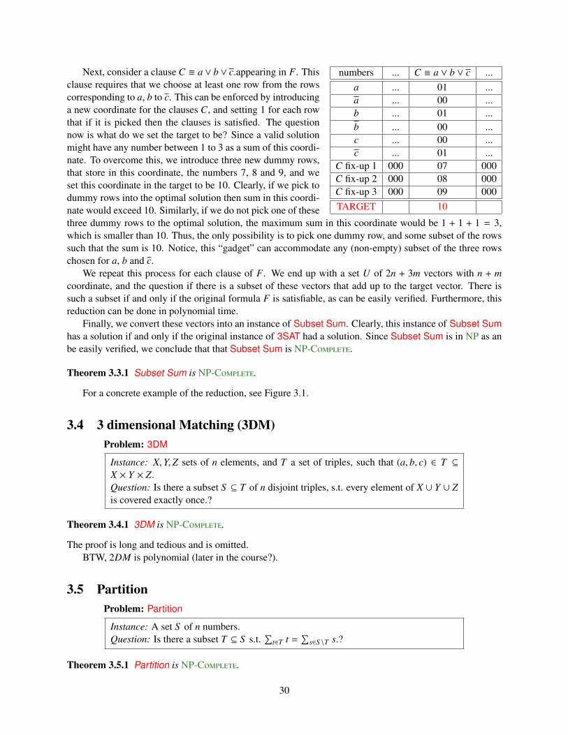
numbers ... C ≡ a ∨ b ∨ c ...a ... 01 ...a ... 00 ...b ... 01 ...b ... 00 ...c ... 00 ...c ... 01 ...

C fix-up 1 000 07 000C fix-up 2 000 08 000C fix-up 3 000 09 000TARGET 10

Next, consider a clause C ≡ a∨ b∨ c.appearing in F. Thisclause requires that we choose at least one row from the rowscorresponding to a, b to c. This can be enforced by introducinga new coordinate for the clauses C, and setting 1 for each rowthat if it is picked then the clauses is satisfied. The questionnow is what do we set the target to be? Since a valid solutionmight have any number between 1 to 3 as a sum of this coordi-nate. To overcome this, we introduce three new dummy rows,that store in this coordinate, the numbers 7, 8 and 9, and weset this coordinate in the target to be 10. Clearly, if we pick todummy rows into the optimal solution then sum in this coordi-nate would exceed 10. Similarly, if we do not pick one of thesethree dummy rows to the optimal solution, the maximum sum in this coordinate would be 1 + 1 + 1 = 3,which is smaller than 10. Thus, the only possibility is to pick one dummy row, and some subset of the rowssuch that the sum is 10. Notice, this “gadget” can accommodate any (non-empty) subset of the three rowschosen for a, b and c.

We repeat this process for each clause of F. We end up with a set U of 2n + 3m vectors with n + mcoordinate, and the question if there is a subset of these vectors that add up to the target vector. There issuch a subset if and only if the original formula F is satisfiable, as can be easily verified. Furthermore, thisreduction can be done in polynomial time.

Finally, we convert these vectors into an instance of Subset Sum. Clearly, this instance of Subset Sumhas a solution if and only if the original instance of 3SAT had a solution. Since Subset Sum is in NP as anbe easily verified, we conclude that that Subset Sum is NP-C.

Theorem 3.3.1 Subset Sum is NP-C.

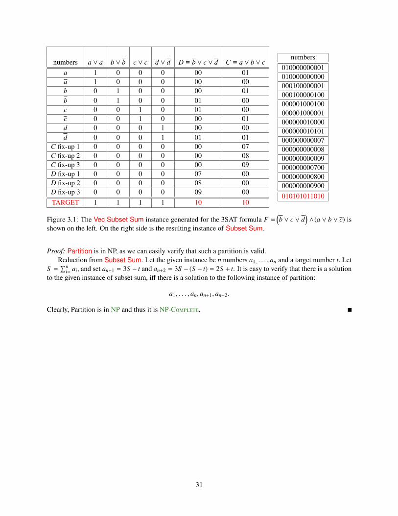
For a concrete example of the reduction, see Figure 3.1.

3.4 3 dimensional Matching (3DM)Problem: 3DM

Instance: X,Y,Z sets of n elements, and T a set of triples, such that (a, b, c) ∈ T ⊆X × Y × Z.Question: Is there a subset S ⊆ T of n disjoint triples, s.t. every element of X ∪ Y ∪ Zis covered exactly once.?

Theorem 3.4.1 3DM is NP-C.

The proof is long and tedious and is omitted.BTW, 2DM is polynomial (later in the course?).

3.5 PartitionProblem: Partition

Instance: A set S of n numbers.Question: Is there a subset T ⊆ S s.t.

∑t∈T t =

∑s∈S \T s.?

Theorem 3.5.1 Partition is NP-C.

30

numbers a ∨ a b ∨ b c ∨ c d ∨ d D ≡ b ∨ c ∨ d C ≡ a ∨ b ∨ ca 1 0 0 0 00 01a 1 0 0 0 00 00b 0 1 0 0 00 01b 0 1 0 0 01 00c 0 0 1 0 01 00c 0 0 1 0 00 01d 0 0 0 1 00 00d 0 0 0 1 01 01

C fix-up 1 0 0 0 0 00 07C fix-up 2 0 0 0 0 00 08C fix-up 3 0 0 0 0 00 09D fix-up 1 0 0 0 0 07 00D fix-up 2 0 0 0 0 08 00D fix-up 3 0 0 0 0 09 00TARGET 1 1 1 1 10 10

numbers010000000001010000000000000100000001000100000100000001000100000001000001000000010000000000010101000000000007000000000008000000000009000000000700000000000800000000000900010101011010

Figure 3.1: The Vec Subset Sum instance generated for the 3SAT formula F =(b ∨ c ∨ d

)∧(a ∨ b ∨ c) is

shown on the left. On the right side is the resulting instance of Subset Sum.

Proof: Partition is in NP, as we can easily verify that such a partition is valid.Reduction from Subset Sum. Let the given instance be n numbers a1, . . . , an and a target number t. Let

S =∑n

i= ai, and set an+1 = 3S − t and an+2 = 3S − (S − t) = 2S + t. It is easy to verify that there is a solutionto the given instance of subset sum, iff there is a solution to the following instance of partition:

a1, . . . , an, an+1, an+2.

Clearly, Partition is in NP and thus it is NP-C.

31

32

Chapter 4

Dynamic programming

The events of 8 September prompted Foch to draft the later legendary signal: “My centre is giving way, my right isin retreat, situation excellent. I attack.” It was probably never sent.

– – The first world war, John Keegan.

4.1 Basic Idea - Partition Number

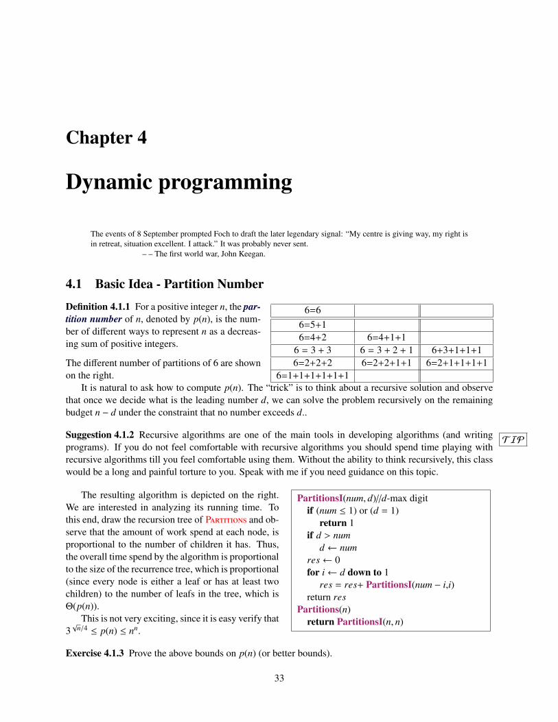
6=66=5+16=4+2 6=4+1+1

6 = 3 + 3 6 = 3 + 2 + 1 6+3+1+1+16=2+2+2 6=2+2+1+1 6=2+1+1+1+1

6=1+1+1+1+1+1

Definition 4.1.1 For a positive integer n, the par-tition number of n, denoted by p(n), is the num-ber of different ways to represent n as a decreas-ing sum of positive integers.

The different number of partitions of 6 are shownon the right.

It is natural to ask how to compute p(n). The “trick” is to think about a recursive solution and observethat once we decide what is the leading number d, we can solve the problem recursively on the remainingbudget n − d under the constraint that no number exceeds d..

TIPSuggestion 4.1.2 Recursive algorithms are one of the main tools in developing algorithms (and writingprograms). If you do not feel comfortable with recursive algorithms you should spend time playing withrecursive algorithms till you feel comfortable using them. Without the ability to think recursively, this classwould be a long and painful torture to you. Speak with me if you need guidance on this topic.

PartitionsI(num, d)//d-max digitif (num ≤ 1) or (d = 1)

return 1if d > num

d ← numres← 0for i← d down to 1

res = res+ PartitionsI(num − i,i)return res

Partitions(n)return PartitionsI(n, n)

The resulting algorithm is depicted on the right.We are interested in analyzing its running time. Tothis end, draw the recursion tree of P and ob-serve that the amount of work spend at each node, isproportional to the number of children it has. Thus,the overall time spend by the algorithm is proportionalto the size of the recurrence tree, which is proportional(since every node is either a leaf or has at least twochildren) to the number of leafs in the tree, which isΘ(p(n)).

This is not very exciting, since it is easy verify that3√

n/4 ≤ p(n) ≤ nn.

Exercise 4.1.3 Prove the above bounds on p(n) (or better bounds).

33

TIPSuggestion 4.1.4 Exercises in the class notes are a natural easy questions for inclusions in exams. Youprobably want to spend time doing them.

In fact, Hardy and Ramanujan (in 1918) showed that p(n) ≈ eπ√

2n/3

4n√

3(which I am sure was your first

guess).It is natural to ask, if there is a faster algorithm. Or more specifically, why is the algorithm Partitions

so slowwwwwwwwwwwwwwwwww? The answer is that during the computation of Partitions(n) thefunction PartitionsI(num,max_digit) is called a lot of times with the same parameters.

PartitionsI_C(num,max_digit)if (num ≤ 1) or (max_digit = 1)

return 1if max_digit > num

d ← numif 〈num,max_digit〉 in cache

return cache(〈num,max_digit〉)res← 0for i← max_digit down to 1 do

res += PartitionsI_C(num − i,i)cache(〈num,max_digit〉)← resreturn res

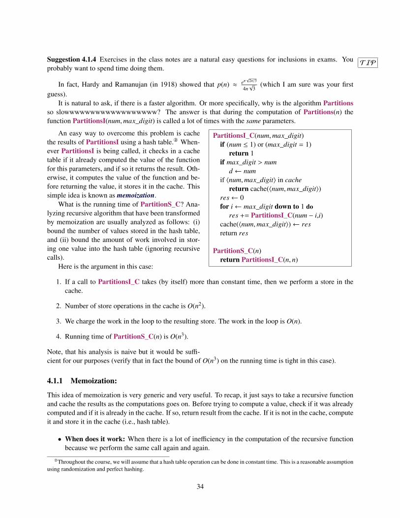
PartitionS_C(n)return PartitionsI_C(n, n)

An easy way to overcome this problem is cachethe results of PartitionsI using a hash table. When-ever PartitionsI is being called, it checks in a cachetable if it already computed the value of the functionfor this parameters, and if so it returns the result. Oth-erwise, it computes the value of the function and be-fore returning the value, it stores it in the cache. Thissimple idea is known as memoization.

What is the running time of PartitionS_C? Ana-lyzing recursive algorithm that have been transformedby memoization are usually analyzed as follows: (i)bound the number of values stored in the hash table,and (ii) bound the amount of work involved in stor-ing one value into the hash table (ignoring recursivecalls).

Here is the argument in this case:

1. If a call to PartitionsI_C takes (by itself) more than constant time, then we perform a store in thecache.

2. Number of store operations in the cache is O(n2).

3. We charge the work in the loop to the resulting store. The work in the loop is O(n).

4. Running time of PartitionS_C(n) is O(n3).

Note, that his analysis is naive but it would be suffi-cient for our purposes (verify that in fact the bound of O(n3) on the running time is tight in this case).

4.1.1 Memoization:

This idea of memoization is very generic and very useful. To recap, it just says to take a recursive functionand cache the results as the computations goes on. Before trying to compute a value, check if it was alreadycomputed and if it is already in the cache. If so, return result from the cache. If it is not in the cache, computeit and store it in the cache (i.e., hash table).

• When does it work: When there is a lot of inefficiency in the computation of the recursive functionbecause we perform the same call again and again.

Throughout the course, we will assume that a hash table operation can be done in constant time. This is a reasonable assumptionusing randomization and perfect hashing.

34

• When it does NOT work:

1. When the number of different recursive function calls (i.e., the different values of the parametersin the recursive call) is “large”.

2. When the function has side effects.

tidbitTidbit 4.1.5 Some functional programming languages allow one to take a recursive function f (·) that youalready implemented and give you a memorized version f ′(·) of this function without the programmer doingany extra work. For a nice description of how to implement it in Scheme see [ASS96].

It is natural to ask if we can do better than just than caching? As usual in life – more pain, more gain.Indeed, in a lot of cases we can analyze the recursive calls, and store them directly in an (multi-dimensional)array. This gets rid of the recursion (which used to be an important thing long time ago when memory usedby the stack was a truly limited resource, but it is less important nowadays) which usually yields a slightimprovement in performance.

This technique is known as dynamic programming. We can sometime save space and improve runningtime in dynamic programming over memoization.

Dynamic programing made easy.

1. Solve the problem using recursion - easy (?).

2. Modify the recursive program so that it caches the results.

3. Dynamic programming: Modify the cache into an array.

4.2 Fibonacci numbers

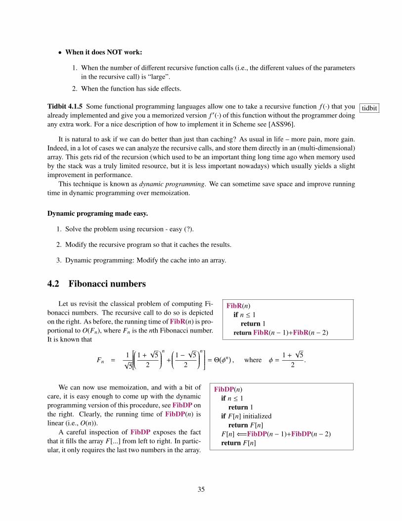
FibR(n)if n ≤ 1

return 1return FibR(n − 1)+FibR(n − 2)

Let us revisit the classical problem of computing Fi-bonacci numbers. The recursive call to do so is depictedon the right. As before, the running time of FibR(n) is pro-portional to O(Fn), where Fn is the nth Fibonacci number.It is known that

Fn =1√

5

1 +√

52

n

+

1 −√

52

n = Θ(φn) , where φ =1 +√

52

.

FibDP(n)if n ≤ 1

return 1if F[n] initialized

return F[n]F[n]⇐=FibDP(n − 1)+FibDP(n − 2)return F[n]

We can now use memoization, and with a bit ofcare, it is easy enough to come up with the dynamicprogramming version of this procedure, see FibDP onthe right. Clearly, the running time of FibDP(n) islinear (i.e., O(n)).

A careful inspection of FibDP exposes the factthat it fills the array F[...] from left to right. In partic-ular, it only requires the last two numbers in the array.

35

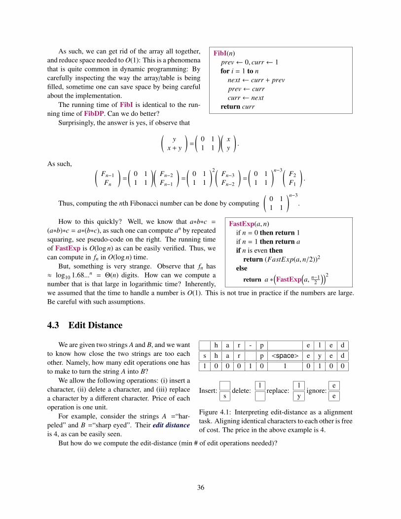
FibI(n)prev← 0, curr ← 1for i = 1 to n

next ← curr + prevprev← currcurr ← next

return curr

As such, we can get rid of the array all together,and reduce space needed to O(1): This is a phenomenathat is quite common in dynamic programming: Bycarefully inspecting the way the array/table is beingfilled, sometime one can save space by being carefulabout the implementation.

The running time of FibI is identical to the run-ning time of FibDP. Can we do better?

Surprisingly, the answer is yes, if observe that(y

x + y

)=

(0 11 1

)(xy

).

As such, (Fn−1Fn

)=

(0 11 1

)(Fn−2Fn−1

)=

(0 11 1

)2( Fn−3Fn−2

)=

(0 11 1

)n−3( F2F1

).

Thus, computing the nth Fibonacci number can be done by computing(

0 11 1

)n−3

.

FastExp(a, n)if n = 0 then return 1if n = 1 then return aif n is even then

return (FastExp(a, n/2))2

elsereturn a ∗

(FastExp

(a, n−1

2

))2

How to this quickly? Well, we know that a∗b∗c =(a∗b)∗c = a∗(b∗c), as such one can compute an by repeatedsquaring, see pseudo-code on the right. The running timeof FastExp is O(log n) as can be easily verified. Thus, wecan compute in fn in O(log n) time.

But, something is very strange. Observe that fn has≈ log10 1.68...n = Θ(n) digits. How can we compute anumber that is that large in logarithmic time? Inherently,we assumed that the time to handle a number is O(1). This is not true in practice if the numbers are large.Be careful with such assumptions.

4.3 Edit Distance

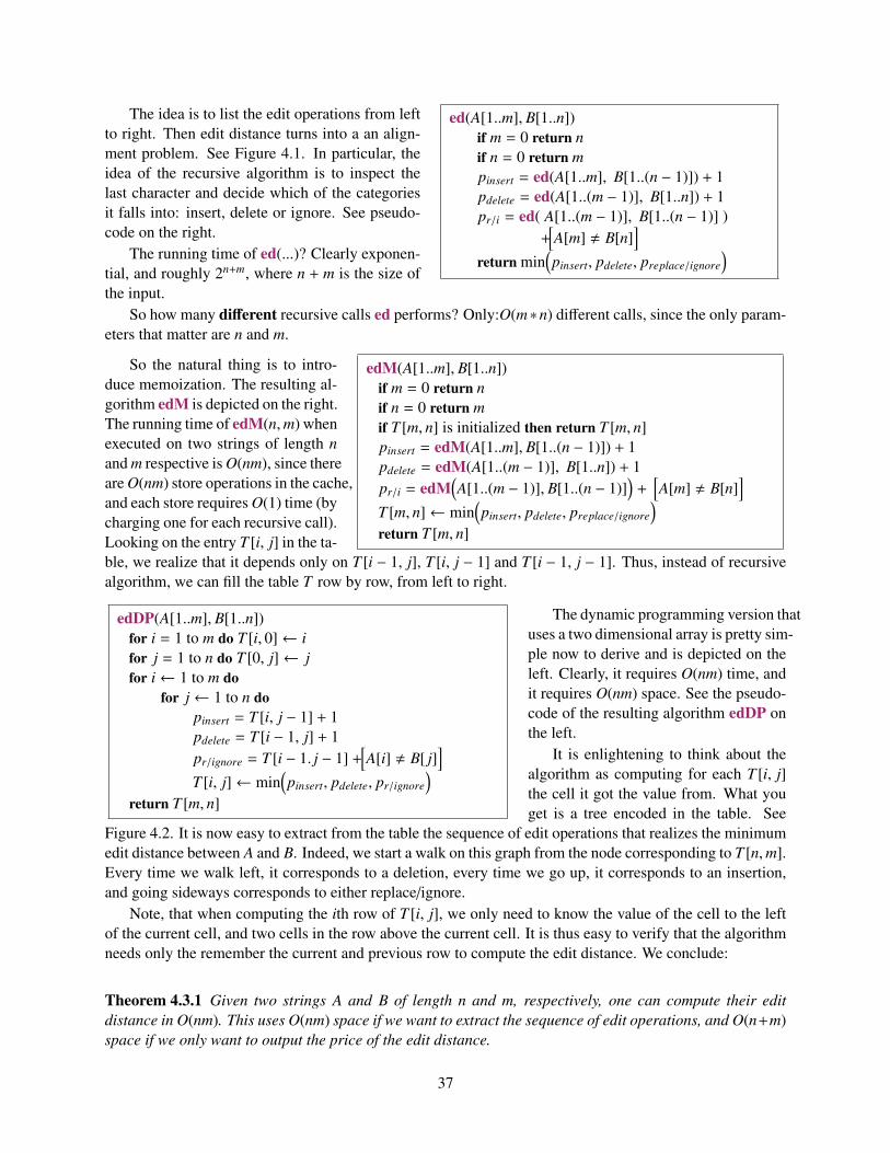
h a r - p e l e ds h a r p <space> e y e d1 0 0 0 1 0 1 0 1 0 0

Insert:s

delete:l

replace:ly

ignore:ee

Figure 4.1: Interpreting edit-distance as a alignmenttask. Aligning identical characters to each other is freeof cost. The price in the above example is 4.

We are given two strings A and B, and we wantto know how close the two strings are too eachother. Namely, how many edit operations one hasto make to turn the string A into B?

We allow the following operations: (i) insert acharacter, (ii) delete a character, and (iii) replacea character by a different character. Price of eachoperation is one unit.

For example, consider the strings A =“har-peled” and B =“sharp eyed”. Their edit distanceis 4, as can be easily seen.

But how do we compute the edit-distance (min # of edit operations needed)?

36

ed(A[1..m], B[1..n])if m = 0 return nif n = 0 return mpinsert = ed(A[1..m], B[1..(n − 1)]) + 1pdelete = ed(A[1..(m − 1)], B[1..n]) + 1pr/i = ed( A[1..(m − 1)], B[1..(n − 1)] )

+[A[m] , B[n]

]return min

(pinsert, pdelete, preplace/ignore

)

The idea is to list the edit operations from leftto right. Then edit distance turns into a an align-ment problem. See Figure 4.1. In particular, theidea of the recursive algorithm is to inspect thelast character and decide which of the categoriesit falls into: insert, delete or ignore. See pseudo-code on the right.

The running time of ed(...)? Clearly exponen-tial, and roughly 2n+m, where n + m is the size ofthe input.

So how many different recursive calls ed performs? Only:O(m∗n) different calls, since the only param-eters that matter are n and m.

edM(A[1..m], B[1..n])if m = 0 return nif n = 0 return mif T [m, n] is initialized then return T [m, n]pinsert = edM(A[1..m], B[1..(n − 1)]) + 1pdelete = edM(A[1..(m − 1)], B[1..n]) + 1pr/i = edM

(A[1..(m − 1)], B[1..(n − 1)]

)+

[A[m] , B[n]

]T [m, n]← min

(pinsert, pdelete, preplace/ignore

)return T [m, n]

So the natural thing is to intro-duce memoization. The resulting al-gorithm edM is depicted on the right.The running time of edM(n,m) whenexecuted on two strings of length nand m respective is O(nm), since thereare O(nm) store operations in the cache,and each store requires O(1) time (bycharging one for each recursive call).Looking on the entry T [i, j] in the ta-ble, we realize that it depends only on T [i − 1, j], T [i, j − 1] and T [i − 1, j − 1]. Thus, instead of recursivealgorithm, we can fill the table T row by row, from left to right.

edDP(A[1..m], B[1..n])for i = 1 to m do T [i, 0]← ifor j = 1 to n do T [0, j]← jfor i← 1 to m do

for j← 1 to n dopinsert = T [i, j − 1] + 1pdelete = T [i − 1, j] + 1pr/ignore = T [i − 1. j − 1] +

[A[i] , B[ j]

]T [i, j]← min

(pinsert, pdelete, pr/ignore

)return T [m, n]

The dynamic programming version thatuses a two dimensional array is pretty sim-ple now to derive and is depicted on theleft. Clearly, it requires O(nm) time, andit requires O(nm) space. See the pseudo-code of the resulting algorithm edDP onthe left.

It is enlightening to think about thealgorithm as computing for each T [i, j]the cell it got the value from. What youget is a tree encoded in the table. See

Figure 4.2. It is now easy to extract from the table the sequence of edit operations that realizes the minimumedit distance between A and B. Indeed, we start a walk on this graph from the node corresponding to T [n,m].Every time we walk left, it corresponds to a deletion, every time we go up, it corresponds to an insertion,and going sideways corresponds to either replace/ignore.

Note, that when computing the ith row of T [i, j], we only need to know the value of the cell to the leftof the current cell, and two cells in the row above the current cell. It is thus easy to verify that the algorithmneeds only the remember the current and previous row to compute the edit distance. We conclude:

Theorem 4.3.1 Given two strings A and B of length n and m, respectively, one can compute their editdistance in O(nm). This uses O(nm) space if we want to extract the sequence of edit operations, and O(n+m)space if we only want to output the price of the edit distance.

37

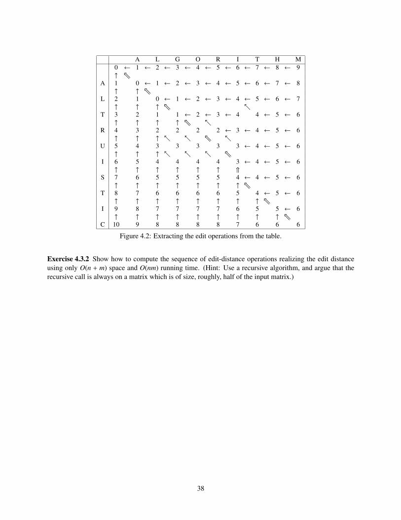
A L G O R I T H M0 ← 1 ← 2 ← 3 ← 4 ← 5 ← 6 ← 7 ← 8 ← 9↑ v

A 1 0 ← 1 ← 2 ← 3 ← 4 ← 5 ← 6 ← 7 ← 8↑ ↑ v

L 2 1 0 ← 1 ← 2 ← 3 ← 4 ← 5 ← 6 ← 7↑ ↑ ↑ v

T 3 2 1 1 ← 2 ← 3 ← 4 4 ← 5 ← 6↑ ↑ ↑ ↑ v

R 4 3 2 2 2 2 ← 3 ← 4 ← 5 ← 6↑ ↑ ↑ v

U 5 4 3 3 3 3 3 ← 4 ← 5 ← 6↑ ↑ ↑ v

I 6 5 4 4 4 4 3 ← 4 ← 5 ← 6↑ ↑ ↑ ↑ ↑ ↑ ⇑

S 7 6 5 5 5 5 4 ← 4 ← 5 ← 6↑ ↑ ↑ ↑ ↑ ↑ ↑ v

T 8 7 6 6 6 6 5 4 ← 5 ← 6↑ ↑ ↑ ↑ ↑ ↑ ↑ ↑ v

I 9 8 7 7 7 7 6 5 5 ← 6↑ ↑ ↑ ↑ ↑ ↑ ↑ ↑ ↑ v

C 10 9 8 8 8 8 7 6 6 6

Figure 4.2: Extracting the edit operations from the table.

Exercise 4.3.2 Show how to compute the sequence of edit-distance operations realizing the edit distanceusing only O(n + m) space and O(nm) running time. (Hint: Use a recursive algorithm, and argue that therecursive call is always on a matrix which is of size, roughly, half of the input matrix.)

38

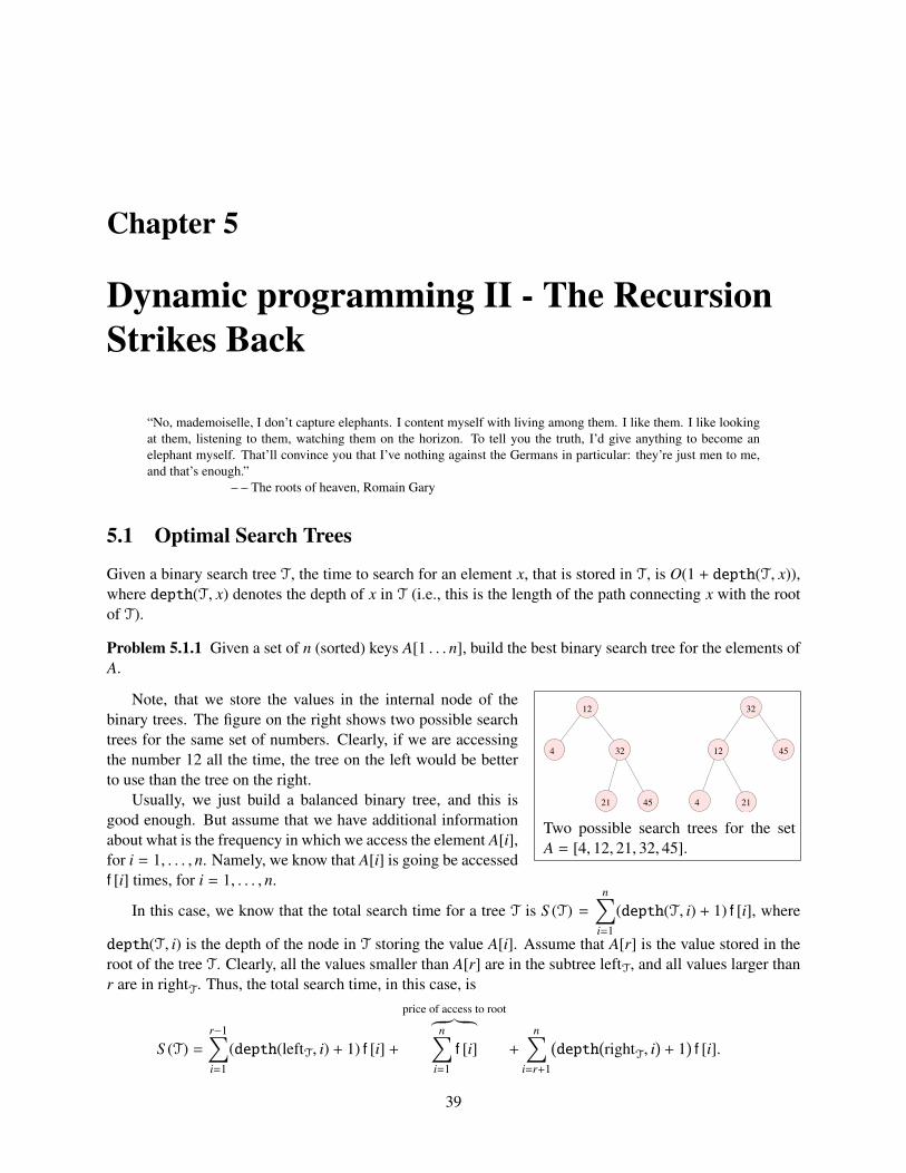
Chapter 5

Dynamic programming II - The RecursionStrikes Back

“No, mademoiselle, I don’t capture elephants. I content myself with living among them. I like them. I like lookingat them, listening to them, watching them on the horizon. To tell you the truth, I’d give anything to become anelephant myself. That’ll convince you that I’ve nothing against the Germans in particular: they’re just men to me,and that’s enough.”

– – The roots of heaven, Romain Gary

5.1 Optimal Search Trees

Given a binary search tree T, the time to search for an element x, that is stored in T, is O(1 + depth(T, x)),where depth(T, x) denotes the depth of x in T (i.e., this is the length of the path connecting x with the rootof T).

Problem 5.1.1 Given a set of n (sorted) keys A[1 . . . n], build the best binary search tree for the elements ofA.

4

12

21

32

45

45

32

12

4 21

Two possible search trees for the setA = [4, 12, 21, 32, 45].

Note, that we store the values in the internal node of thebinary trees. The figure on the right shows two possible searchtrees for the same set of numbers. Clearly, if we are accessingthe number 12 all the time, the tree on the left would be betterto use than the tree on the right.

Usually, we just build a balanced binary tree, and this isgood enough. But assume that we have additional informationabout what is the frequency in which we access the element A[i],for i = 1, . . . , n. Namely, we know that A[i] is going be accessedf [i] times, for i = 1, . . . , n.

In this case, we know that the total search time for a tree T is S (T) =n∑

i=1

(depth(T, i) + 1) f [i], where

depth(T, i) is the depth of the node in T storing the value A[i]. Assume that A[r] is the value stored in theroot of the tree T. Clearly, all the values smaller than A[r] are in the subtree leftT , and all values larger thanr are in rightT . Thus, the total search time, in this case, is

S (T) =r−1∑i=1

(depth(leftT , i) + 1) f [i] +

price of access to root︷︸︸︷n∑

i=1

f [i] +

n∑i=r+1

(depth

(rightT , i

)+ 1

)f [i].

39

Observe, that if T is the optimal search tree for the access frequencies f [1], . . . , f [n], then The subtreeleftT must be optimal for the elements accessing it (i.e., A[1 . . . r − 1] where r is the root).

Thus, the price of T is

S (T) = S (leftT ) + S (rightT ) +n∑

i=1

f [i],

where S (Q) is the price of searching in Q for the frequency of elements stored in Q.

CompBestTreeI(A[i . . . j], f

[i . . . j

] )for r = i . . . j do

Tle f t ← CompBestTreeI(A[i . . . r − 1], f [i . . . r − 1])Tright ← CompBestTreeI(A[r + 1 . . . j], f

[r + 1 . . . j

])

Tr ← Tree(Tle f t , A[r] , Tright

)Pr ← S (Tr)

return cheapest tree out of Ti, . . . ,T j.

CompBestTree(A[1 . . . n], f [1 . . . n]

)return CompBestTreeI( A[1 . . . n], f [1 . . . n])

This recursive formula naturally givesrise to a recursive algorithm, which is de-picted on the right. The naive implemen-tation requires O(n2) time (ignoring therecursive call). But in fact, by a morecareful implementation, together with thetree T, we can also return the price ofsearching on this tree with the given fre-quencies. Thus, this modified algorithm.Thus, the running time for this functiontakes O(n) time (ignoring recursive calls).The running time of the resulting algo-rithm is

α(n) = O(n) +n−1∑i=0

(α(i) + α(n − i − 1)) ,

and the solution of this recurrence is O(n3n) .We can, of course, improve the running time using memoization. There are only O(n2) different recursive

calls, and as such, the running time of CompBestTreeMemoize is O(n2) · O(n) = O(n3).

Theorem 5.1.2 Can can compute the optimal binary search tree in O(n3

)time using O

(n2

)space.

A further improvement raises from the fact that the root location is “monotone”. Formally, if R[i, j]denotes the location of the element stored in the root for the elements A[i . . . j] then it holds that R[i, j−1] ≤R[i, j] ≤ R[i, j + 1]. This limits the search space, and we can be more efficient in the search. This leads toO(n2

)algorithm. Details are in Jeff Erickson class notes.

5.2 Optimal Triangulations

Given a convex polygon P in the plane, we would like to find the triangulation of P of minimum total length.Namely, the total length of the diagonals of the triangulation of P, plus the (length of the) perimeter of P areminimized. See Figure 5.1.

Definition 5.2.1 A set S ⊆ IRd is convex if for any to x, y ∈ S , the segment xy is contained in S .A convex polygon is a closed cycle of segments, with no vertex pointing inward. Formally, it is a simple

closed polygonal curve which encloses a convex set.A diagonal is a line segment connecting two vertices of a polygon which are not adjacent. A triangula-

tion is a partition of a convex polygon into (interior) disjoint triangles using diagonals.

Observation 5.2.2 Any triangulation of a convex polygon with n vertices is made out of exactly n − 2triangles.

40

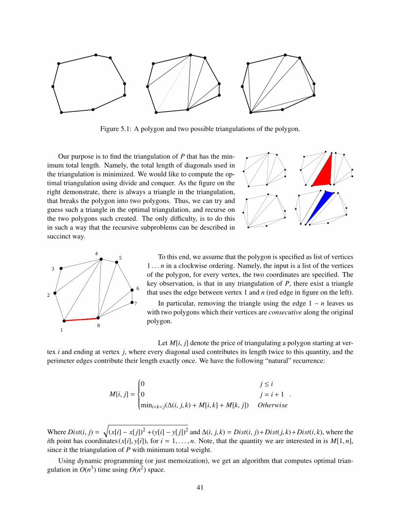
Figure 5.1: A polygon and two possible triangulations of the polygon.

Our purpose is to find the triangulation of P that has the min-imum total length. Namely, the total length of diagonals used inthe triangulation is minimized. We would like to compute the op-timal triangulation using divide and conquer. As the figure on theright demonstrate, there is always a triangle in the triangulation,that breaks the polygon into two polygons. Thus, we can try andguess such a triangle in the optimal triangulation, and recurse onthe two polygons such created. The only difficulty, is to do thisin such a way that the recursive subproblems can be described insuccinct way.

1

2

3

45

6

7

8

To this end, we assume that the polygon is specified as list of vertices1 . . . n in a clockwise ordering. Namely, the input is a list of the verticesof the polygon, for every vertex, the two coordinates are specified. Thekey observation, is that in any triangulation of P, there exist a trianglethat uses the edge between vertex 1 and n (red edge in figure on the left).

In particular, removing the triangle using the edge 1 − n leaves uswith two polygons which their vertices are consecutive along the originalpolygon.

Let M[i, j] denote the price of triangulating a polygon starting at ver-tex i and ending at vertex j, where every diagonal used contributes its length twice to this quantity, and theperimeter edges contribute their length exactly once. We have the following “natural” recurrence:

M[i, j] =

0 j ≤ i0 j = i + 1mini<k< j(∆(i, j, k) + M[i, k] + M[k, j]) Otherwise

.

Where Dist(i, j) =√

(x[i] − x[ j])2 +(y[i] − y[ j])2 and ∆(i, j, k) = Dist(i, j)+Dist( j, k)+Dist(i, k), where theith point has coordinates (x[i], y[i]), for i = 1, . . . , n. Note, that the quantity we are interested in is M[1, n],since it the triangulation of P with minimum total weight.

Using dynamic programming (or just memoization), we get an algorithm that computes optimal trian-gulation in O(n3) time using O(n2) space.

41

5.3 Matrix Multiplication

We are given two matrix: (i) A is a matrix with dimensions p × q (i.e., p rows and q columns) and (ii) B is amatrix of size q × r. The product matrix AB, with dimensions p × r, can be computed in O(pqr) time usingthe standard algorithm.

A 1000 × 2B 2 × 1000C 1000 × 2

Things becomes considerably more interesting when we have to multiply a chain formatrices. Consider for example the three matrices A, B and C with dimensions as listedon the left. Computing the matrix ABC = A(BC) requires 2 · 1000 · 2 + 1000 · 2 · 2 =8, 000 operations. On the other hand, computing the same matrix using (AB)C requires

1000 · 2 · 1000 + 1000 · 1000 · 2 = 4, 000, 000. Note, that matrix multiplication is associative, and as such(AB)C = A(BC).

Thus, given a chain of matrices that we need to multiply, the exact ordering in which we do the multi-plication matters as far to multiply the order is important as far as efficiency.

Problem 5.3.1 The input is n matrices M1, . . . ,Mn such that Mi is of size D[i−1]×D[i] (i.e., Mi has D[i−1]rows and D[i] columns), where D[0 . . . n] is array specifying the sizes. Find the ordering of multiplicationsto compute M1 · M2 · · ·Mn−1 · Mn most efficiently.

Again, let us define a recurrence for this problem, where M[i, j] is the amount of work involved incomputing the product of the matrices Mi · · ·M j. We have

M[i, j] =

0 j = iD[i − 1] · D[i] · D[i + 1] j = i + 1mini≤k< j(M[i, k] + M[k + 1, j] + D[i − 1] · D[k] · D[ j]) j > i + 1.

Again, using memoization (or dynamic programming), one can compute M[1, n], in O(n3) time, usingO(n2) space.

5.4 Longest Ascending Subsequence

Given an array of numbers A[1 . . . n] we are interested in finding the longest ascending subsequence. Forexample, if A = [6, 3, 2, 5, 1, 12] the longest ascending subsequence is 2, 5, 12. This this end, let M[i] denotelongest increasing subsequence having A[i] as the last element in the subsequence. The recurrence on themaximum possible length, is

M[n] =

1 n = 11 + max

1≤k<n,A[k]<A[n]M[k] otherwise.

The length of the longest increasing subsequence is maxni=1 M[i]. Again, using dynamic programming,

we get an algorithm with running time O(n2) for this problem. It is also not hard to modify the algorithmso that it outputs this sequence (you should figure out the details of this modification). A better O(n log n)solution is possible using some data-structure magic.

5.5 Pattern Matching

42

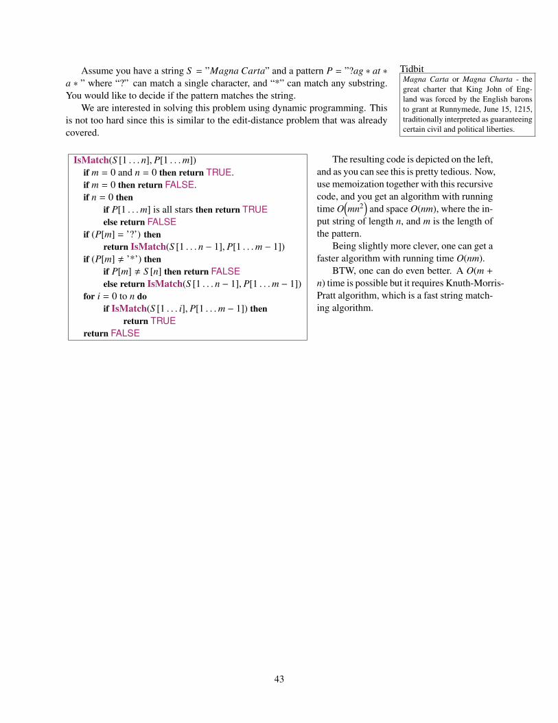
TidbitMagna Carta or Magna Charta - thegreat charter that King John of Eng-land was forced by the English baronsto grant at Runnymede, June 15, 1215,traditionally interpreted as guaranteeingcertain civil and political liberties.

Assume you have a string S = ”Magna Carta” and a pattern P = ”?ag ∗ at ∗a ∗ ” where “?” can match a single character, and “*” can match any substring.You would like to decide if the pattern matches the string.

We are interested in solving this problem using dynamic programming. Thisis not too hard since this is similar to the edit-distance problem that was alreadycovered.

IsMatch(S [1 . . . n], P[1 . . .m])if m = 0 and n = 0 then return TRUE.if m = 0 then return FALSE.if n = 0 then

if P[1 . . .m] is all stars then return TRUEelse return FALSE

if (P[m] = ’?’) thenreturn IsMatch(S [1 . . . n − 1], P[1 . . .m − 1])

if (P[m] , ’*’) thenif P[m] , S [n] then return FALSEelse return IsMatch(S [1 . . . n − 1], P[1 . . .m − 1])

for i = 0 to n doif IsMatch(S [1 . . . i], P[1 . . .m − 1]) then

return TRUEreturn FALSE

The resulting code is depicted on the left,and as you can see this is pretty tedious. Now,use memoization together with this recursivecode, and you get an algorithm with runningtime O

(mn2

)and space O(nm), where the in-

put string of length n, and m is the length ofthe pattern.

Being slightly more clever, one can get afaster algorithm with running time O(nm).

BTW, one can do even better. A O(m +n) time is possible but it requires Knuth-Morris-Pratt algorithm, which is a fast string match-ing algorithm.

43

44

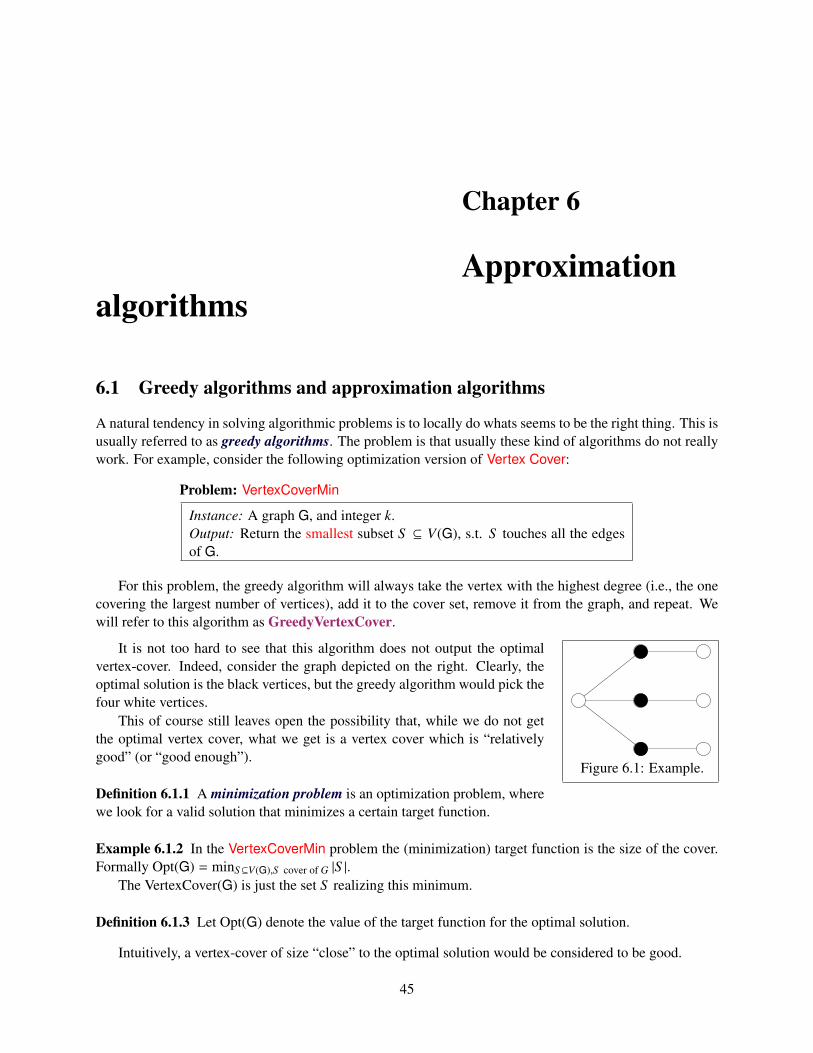
Chapter 6

Approximationalgorithms

6.1 Greedy algorithms and approximation algorithms

A natural tendency in solving algorithmic problems is to locally do whats seems to be the right thing. This isusually referred to as greedy algorithms. The problem is that usually these kind of algorithms do not reallywork. For example, consider the following optimization version of Vertex Cover:

Problem: VertexCoverMin

Instance: A graph G, and integer k.Output: Return the smallest subset S ⊆ V(G), s.t. S touches all the edgesof G.

For this problem, the greedy algorithm will always take the vertex with the highest degree (i.e., the onecovering the largest number of vertices), add it to the cover set, remove it from the graph, and repeat. Wewill refer to this algorithm as GreedyVertexCover.

Figure 6.1: Example.

It is not too hard to see that this algorithm does not output the optimalvertex-cover. Indeed, consider the graph depicted on the right. Clearly, theoptimal solution is the black vertices, but the greedy algorithm would pick thefour white vertices.

This of course still leaves open the possibility that, while we do not getthe optimal vertex cover, what we get is a vertex cover which is “relativelygood” (or “good enough”).

Definition 6.1.1 A minimization problem is an optimization problem, wherewe look for a valid solution that minimizes a certain target function.

Example 6.1.2 In the VertexCoverMin problem the (minimization) target function is the size of the cover.Formally Opt(G) = minS⊆V(G),S cover of G |S |.

The VertexCover(G) is just the set S realizing this minimum.

Definition 6.1.3 Let Opt(G) denote the value of the target function for the optimal solution.

Intuitively, a vertex-cover of size “close” to the optimal solution would be considered to be good.

45

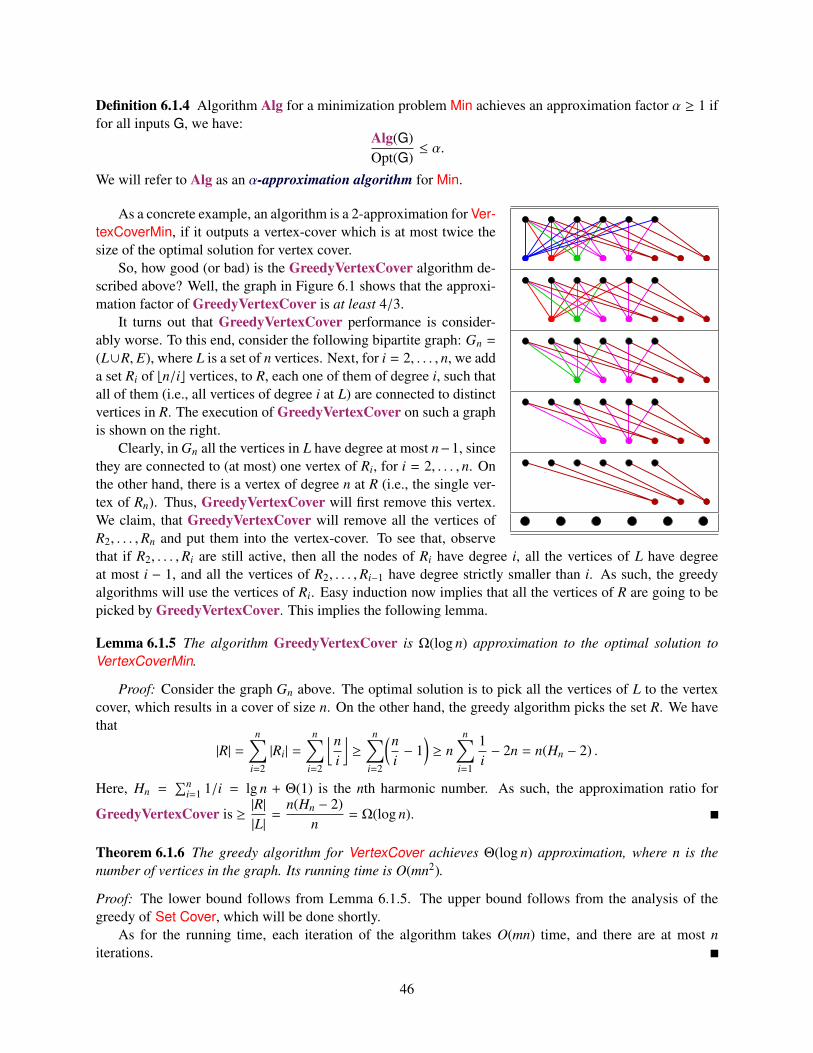
Definition 6.1.4 Algorithm Alg for a minimization problem Min achieves an approximation factor α ≥ 1 iffor all inputs G, we have:

Alg(G)Opt(G)

≤ α.

We will refer to Alg as an α-approximation algorithm for Min.

As a concrete example, an algorithm is a 2-approximation for Ver-texCoverMin, if it outputs a vertex-cover which is at most twice thesize of the optimal solution for vertex cover.

So, how good (or bad) is the GreedyVertexCover algorithm de-scribed above? Well, the graph in Figure 6.1 shows that the approxi-mation factor of GreedyVertexCover is at least 4/3.

It turns out that GreedyVertexCover performance is consider-ably worse. To this end, consider the following bipartite graph: Gn =

(L∪R, E), where L is a set of n vertices. Next, for i = 2, . . . , n, we adda set Ri of bn/ic vertices, to R, each one of them of degree i, such thatall of them (i.e., all vertices of degree i at L) are connected to distinctvertices in R. The execution of GreedyVertexCover on such a graphis shown on the right.

Clearly, in Gn all the vertices in L have degree at most n−1, sincethey are connected to (at most) one vertex of Ri, for i = 2, . . . , n. Onthe other hand, there is a vertex of degree n at R (i.e., the single ver-tex of Rn). Thus, GreedyVertexCover will first remove this vertex.We claim, that GreedyVertexCover will remove all the vertices ofR2, . . . ,Rn and put them into the vertex-cover. To see that, observethat if R2, . . . ,Ri are still active, then all the nodes of Ri have degree i, all the vertices of L have degreeat most i − 1, and all the vertices of R2, . . . ,Ri−1 have degree strictly smaller than i. As such, the greedyalgorithms will use the vertices of Ri. Easy induction now implies that all the vertices of R are going to bepicked by GreedyVertexCover. This implies the following lemma.

Lemma 6.1.5 The algorithm GreedyVertexCover is Ω(log n) approximation to the optimal solution toVertexCoverMin.

Proof: Consider the graph Gn above. The optimal solution is to pick all the vertices of L to the vertexcover, which results in a cover of size n. On the other hand, the greedy algorithm picks the set R. We havethat

|R| =n∑

i=2

|Ri| =

n∑i=2

⌊ni

⌋≥

n∑i=2

(ni− 1

)≥ n

n∑i=1

1i− 2n = n(Hn − 2) .

Here, Hn =∑n

i=1 1/i = lg n + Θ(1) is the nth harmonic number. As such, the approximation ratio for

GreedyVertexCover is ≥|R||L|=

n(Hn − 2)n

= Ω(log n).

Theorem 6.1.6 The greedy algorithm for VertexCover achieves Θ(log n) approximation, where n is thenumber of vertices in the graph. Its running time is O(mn2).

Proof: The lower bound follows from Lemma 6.1.5. The upper bound follows from the analysis of thegreedy of Set Cover, which will be done shortly.

As for the running time, each iteration of the algorithm takes O(mn) time, and there are at most niterations.

46

6.1.1 Alternative algorithm – two for the price of one

One can still do much better than the greedy algorithm in this case. In particular, let ApproxVertexCoverbe the algorithm that chooses an edge from G, add both endpoints to the vertex cover, and removes the twovertices (and all the edges adjacent to these two vertices) from G. This process is repeated till G has noedges. Clearly, the resulting set of vertices is a vertex-cover, since the algorithm removes an edge only if itis being covered by the generated cover.

Theorem 6.1.7 ApproxVertexCover is a 2-approximation algorithm for VertexCoverMin.

Proof: Every edge picked by the algorithm contains at least one vertex of the optimal solution. As such, thecover generated is at most twice larger than the optimal.

6.2 Traveling Salesman Person

We remind the reader that the optimization variant of the TSP problem is the following.

Problem: TSP-Min

Instance: G = (V, E) a complete graph, and ω(e) a cost function definedover the edges of G.Output: The cheapest tour that visits all the vertices of G exactly once.

Theorem 6.2.1 TSP-Min can not be approximated within any factor unless NP = P.

Proof: Consider the reduction from Hamiltonian Cycle into TSP. Given a graph G, which is the inputfor the Hamiltonian cycle, we transform it into an instance of TSP-Min. Specifically, we set the weight ofevery edge to 1 if it was present in the instance of the Hamiltonian cycle, and 2 otherwise. In the resultingcomplete graph, if there is a tour price n then there is a Hamiltonian cycle in the original graph. If on theother hand, there was no cycle in G then the cheapest TSP is of price n + 1.

Instead of 2, let us assign the missing edges in H a weight of cn, for c an arbitrary number. Let H denotethe resulting graph. Clearly, if G does not contain any Hamiltonian cycle in the original graph, then the priceof the TSP-Min in H is at least cn + 1.

Note, that the prices of tours of H are either (i) equal to n if there is a Hamiltonian cycle in G, or (ii)larger than cn + 1 if there is no Hamiltonian cycle in G. As such, if one can do a c-approximation, inpolynomial time, to TSP-Min, then using it on H would yield a tour of price ≤ cn if a tour of price n exists.But a tour of price ≤ cn exists iff G has a Hamiltonian cycle.

Namely, such an approximation algorithm would solve a NP-C problem (i.e., Hamiltonian Cy-cle) in polynomial time.

Note, that Theorem 6.2.1 implies that TSP-Min can not be approximated to within any factor. How-ever, once we add some assumptions to the problem, it becomes much more manageable (at least as far asapproximation).

What the above reduction did, was to take a problem and reduce it into an instance where this is ahuge gap, between the optimal solution, and the second cheapest solution. Next, we argued that if had anapproximation algorithm that has ratio better than the ratio between the two endpoints of this empty interval,then the approximation algorithm, would in polynomial time would be able to decide if there is an optimalsolution.

47

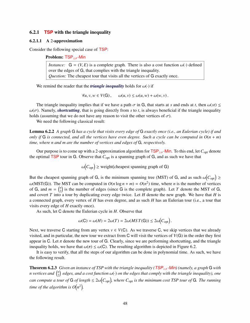
6.2.1 TSP with the triangle inequality

6.2.1.1 A 2-approximation

Consider the following special case of TSP:

Problem: TSP4,-Min

Instance: G = (V, E) is a complete graph. There is also a cost function ω(·) definedover the edges of G, that complies with the triangle inequality.Question: The cheapest tour that visits all the vertices of G exactly once.

We remind the reader that the triangle inequality holds for ω(·) if

∀u, v,w ∈ V(G) , ω(u, v) ≤ ω(u,w) + ω(w, v) .

The triangle inequality implies that if we have a path σ in G, that starts at s and ends at t, then ω(st) ≤ω(σ). Namely, shortcutting, that is going directly from s to t, is always beneficial if the triangle inequalityholds (assuming that we do not have any reason to visit the other vertices of σ).

We need the following classical result:

Lemma 6.2.2 A graph G has a cycle that visits every edge of G exactly once (i.e., an Eulerian cycle) if andonly if G is connected, and all the vertices have even degree. Such a cycle can be computed in O(n + m)time, where n and m are the number of vertices and edges of G, respectively.

Our purpose is to come up with a 2-approximation algorithm for TSP4,-Min. To this end, let Copt denotethe optimal TSP tour in G. Observe that Copt is a spanning graph of G, and as such we have that

ω(Copt

)≥ weight

(cheapest spanning graph of G

)But the cheapest spanning graph of G, is the minimum spanning tree (MST) of G, and as such ω

(Copt

)≥

ω(MST(G)). The MST can be computed in O(n log n + m) = O(n2) time, where n is the number of verticesof G, and m =

(n2

)is the number of edges (since G is the complete graph). Let T denote the MST of G,

and covert T into a tour by duplicating every edge twice. Let H denote the new graph. We have that H isa connected graph, every vertex of H has even degree, and as such H has an Eulerian tour (i.e., a tour thatvisits every edge of H exactly once).

As such, let C denote the Eulerian cycle in H. Observe that

ω(C) = ω(H) = 2ω(T ) = 2ω(MS T (G)) ≤ 2ω(Copt

).

Next, we traverse C starting from any vertex v ∈ V(C). As we traverse C, we skip vertices that we alreadyvisited, and in particular, the new tour we extract from C will visit the vertices of V(G) in the order they firstappear in C. Let π denote the new tour of G. Clearly, since we are performing shortcutting, and the triangleinequality holds, we have that ω(π) ≤ ω(C). The resulting algorithm is depicted in Figure 6.2.

It is easy to verify, that all the steps of our algorithm can be done in polynomial time. As such, we havethe following result.

Theorem 6.2.3 Given an instance of TSP with the triangle inequality (TSP4,-Min) (namely, a graph G withn vertices and

(n2

)edges, and a cost function ω(·) on the edges that comply with the triangle inequality), one

can compute a tour of G of length ≤ 2ω(Copt

), where Copt is the minimum cost TSP tour of G. The running

time of the algorithm is O(n2

).

48

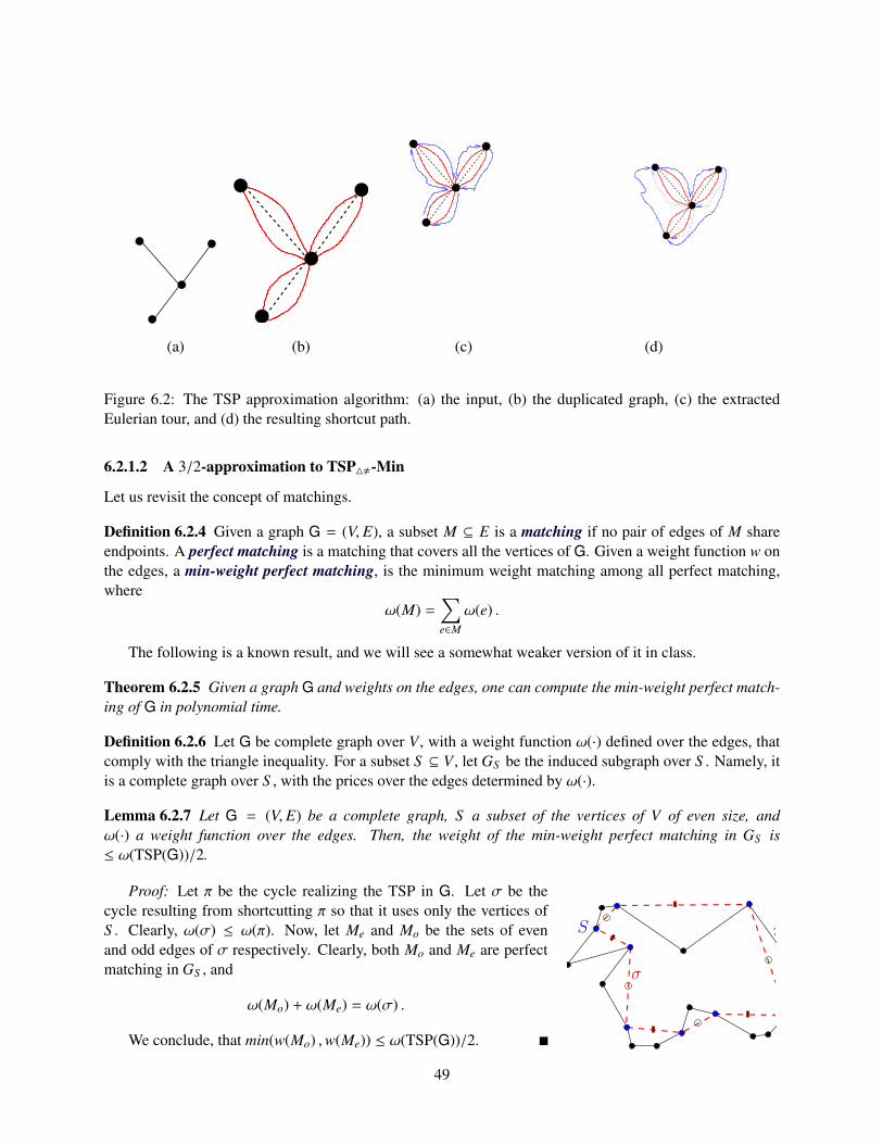
(a) (b) (c) (d)

Figure 6.2: The TSP approximation algorithm: (a) the input, (b) the duplicated graph, (c) the extractedEulerian tour, and (d) the resulting shortcut path.

6.2.1.2 A 3/2-approximation to TSP4,-Min

Let us revisit the concept of matchings.

Definition 6.2.4 Given a graph G = (V, E), a subset M ⊆ E is a matching if no pair of edges of M shareendpoints. A perfect matching is a matching that covers all the vertices of G. Given a weight function w onthe edges, a min-weight perfect matching, is the minimum weight matching among all perfect matching,where

ω(M) =∑e∈M

ω(e) .

The following is a known result, and we will see a somewhat weaker version of it in class.

Theorem 6.2.5 Given a graph G and weights on the edges, one can compute the min-weight perfect match-ing of G in polynomial time.

Definition 6.2.6 Let G be complete graph over V , with a weight function ω(·) defined over the edges, thatcomply with the triangle inequality. For a subset S ⊆ V , let GS be the induced subgraph over S . Namely, itis a complete graph over S , with the prices over the edges determined by ω(·).

Lemma 6.2.7 Let G = (V, E) be a complete graph, S a subset of the vertices of V of even size, andω(·) a weight function over the edges. Then, the weight of the min-weight perfect matching in GS is≤ ω(TSP(G))/2.

σ

πS

Proof: Let π be the cycle realizing the TSP in G. Let σ be thecycle resulting from shortcutting π so that it uses only the vertices ofS . Clearly, ω(σ) ≤ ω(π). Now, let Me and Mo be the sets of evenand odd edges of σ respectively. Clearly, both Mo and Me are perfectmatching in GS , and

ω(Mo) + ω(Me) = ω(σ) .

We conclude, that min(w(Mo) ,w(Me)) ≤ ω(TSP(G))/2.

49

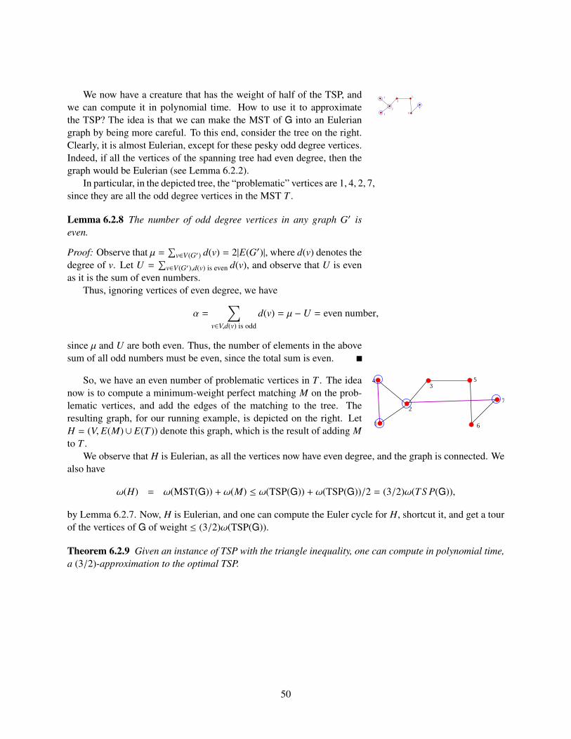
1

4

2

3

5

7

6

We now have a creature that has the weight of half of the TSP, andwe can compute it in polynomial time. How to use it to approximatethe TSP? The idea is that we can make the MST of G into an Euleriangraph by being more careful. To this end, consider the tree on the right.Clearly, it is almost Eulerian, except for these pesky odd degree vertices.Indeed, if all the vertices of the spanning tree had even degree, then thegraph would be Eulerian (see Lemma 6.2.2).

In particular, in the depicted tree, the “problematic” vertices are 1, 4, 2, 7,since they are all the odd degree vertices in the MST T .

Lemma 6.2.8 The number of odd degree vertices in any graph G′ iseven.

Proof: Observe that µ =∑

v∈V(G′) d(v) = 2|E(G′)|, where d(v) denotes thedegree of v. Let U =

∑v∈V(G′),d(v) is even d(v), and observe that U is even

as it is the sum of even numbers.Thus, ignoring vertices of even degree, we have

α =∑

v∈V,d(v) is odd

d(v) = µ − U = even number,

since µ and U are both even. Thus, the number of elements in the abovesum of all odd numbers must be even, since the total sum is even.

1

4

2

35

7

6

So, we have an even number of problematic vertices in T . The ideanow is to compute a minimum-weight perfect matching M on the prob-lematic vertices, and add the edges of the matching to the tree. Theresulting graph, for our running example, is depicted on the right. LetH = (V, E(M)∪ E(T )) denote this graph, which is the result of adding Mto T .

We observe that H is Eulerian, as all the vertices now have even degree, and the graph is connected. Wealso have

ω(H) = ω(MST(G)) + ω(M) ≤ ω(TSP(G)) + ω(TSP(G))/2 = (3/2)ω(TS P(G)),

by Lemma 6.2.7. Now, H is Eulerian, and one can compute the Euler cycle for H, shortcut it, and get a tourof the vertices of G of weight ≤ (3/2)ω(TSP(G)).

Theorem 6.2.9 Given an instance of TSP with the triangle inequality, one can compute in polynomial time,a (3/2)-approximation to the optimal TSP.

50

Chapter 7

Approximation algorithms II

7.1 Max Exact 3SAT

We remind the reader that an instance of 3SAT is a boolean formula, for example F = (x1 + x2 + x3)(x4 +

x1 + x2), and the decision problem is to decide if the formula has a satisfiable assignment. Interestingly, wecan turn this into an optimization problem.

Problem: Max 3SAT

Instance: A collection of clauses: C1, . . . ,Cm.

Output: Find the assignment to x1, ..., xn that satisfies the maximum num-ber of clauses.

Clearly, since 3SAT is NP-C it implies that Max 3SAT is NP-H. In particular, the formula Fbecomes the following set of two clauses:

x1 + x2 + x3 and x4 + x1 + x2.

Note, that Max 3SAT is a maximization problem.

Definition 7.1.1 Algorithm Alg for a maximization problem achieves an approximation factor α if for allinputs, we have:

Alg(G)Opt(G)

≥ α.

In the following, we present a randomized algorithm – it is allowed to consult with a source of randomnumbers in making decisions. A key property we need about random variables, is the linearity of expectationproperty, which is easy to derive directly from the definition of expectation.

Definition 7.1.2 (Linearity of expectations.) Given two random variables X,Y (not necessarily indepen-dent, we have that E[X + Y] = E[X] + E[Y].

Theorem 7.1.3 One can achieve (in expectation) (7/8)-approximation to Max 3SAT in polynomial time.Namely, if the instance has m clauses, then the generated assignment satisfies (7/8)m clauses in expectation.

Proof: Let x1, . . . , xn be the n variables used in the given instance. The algorithm works by randomlyassigning values to x1, . . . , xn, independently, and equal probability, to 0 or 1, for each one of the variables.

51

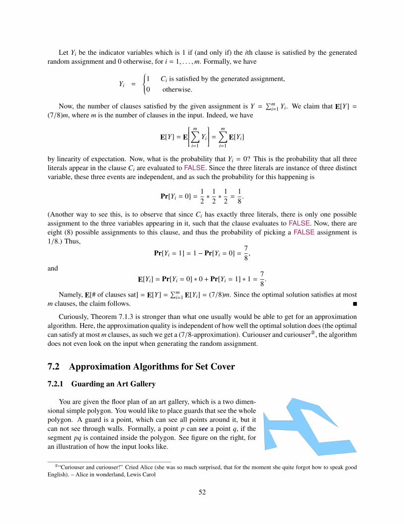
Let Yi be the indicator variables which is 1 if (and only if) the ith clause is satisfied by the generatedrandom assignment and 0 otherwise, for i = 1, . . . ,m. Formally, we have

Yi =

1 Ci is satisfied by the generated assignment,0 otherwise.

Now, the number of clauses satisfied by the given assignment is Y =∑m

i=1 Yi. We claim that E[Y] =(7/8)m, where m is the number of clauses in the input. Indeed, we have

E[Y] = E

m∑i=1

Yi

= m∑i=1

E[Yi]

by linearity of expectation. Now, what is the probability that Yi = 0? This is the probability that all threeliterals appear in the clause Ci are evaluated to FALSE. Since the three literals are instance of three distinctvariable, these three events are independent, and as such the probability for this happening is

Pr[Yi = 0] =12∗

12∗

12=

18.

(Another way to see this, is to observe that since Ci has exactly three literals, there is only one possibleassignment to the three variables appearing in it, such that the clause evaluates to FALSE. Now, there areeight (8) possible assignments to this clause, and thus the probability of picking a FALSE assignment is1/8.) Thus,

Pr[Yi = 1] = 1 − Pr[Yi = 0] =78,

and

E[Yi] = Pr[Yi = 0] ∗ 0 + Pr[Yi = 1] ∗ 1 =78.

Namely, E[# of clauses sat] = E[Y] =∑m

i=1 E[Yi] = (7/8)m. Since the optimal solution satisfies at mostm clauses, the claim follows.

Curiously, Theorem 7.1.3 is stronger than what one usually would be able to get for an approximationalgorithm. Here, the approximation quality is independent of how well the optimal solution does (the optimalcan satisfy at most m clauses, as such we get a (7/8-approximation). Curiouser and curiouser, the algorithmdoes not even look on the input when generating the random assignment.

7.2 Approximation Algorithms for Set Cover

7.2.1 Guarding an Art Gallery

You are given the floor plan of an art gallery, which is a two dimen-sional simple polygon. You would like to place guards that see the wholepolygon. A guard is a point, which can see all points around it, but itcan not see through walls. Formally, a point p can see a point q, if thesegment pq is contained inside the polygon. See figure on the right, foran illustration of how the input looks like.

“Curiouser and curiouser!” Cried Alice (she was so much surprised, that for the moment she quite forgot how to speak goodEnglish). – Alice in wonderland, Lewis Carol

52

p

A visibility polygon at p (depicted as the yellow polygon on the left)is the region inside the polygon that p can see. WE would like to find theminimal number of guards needed to guard the given art-gallery? That is,all the points in the art gallery should be visible from at least one guardwe place.

The art-gallery problem is a set-cover problem. We have a groundset (the polygon), and family of sets (the set of all visibility polygons),

and the target is to find a minimal number of sets covering the whole polygon.It is known that finding the minimum number of guards needed is NP-H. No approximation is

currently known. It is also known that a polygon with n corners, can be guarded using n/3+ 1 guards. Note,that this problem is harder than the classical set-cover problem because the number of subsets is infinite andthe underlining base set is also infinite.

An interesting open problem is to find a polynomial time approximation algorithm, such that given P,it computes a set of guards, such that #guards ≤

√nkopt, where n is the number of vertices of the input

polygon P, and kopt is the number of guards used by the optimal solution.

7.2.2 Set Cover

The optimization version of Set Cover, is the following:

Problem: Set Cover

Instance: (S ,F )S - a set of n elementsF - a family of subsets of S , s.t.

⋃X∈F X = S .

Output: The set X ⊆ F such that X contains as few sets as possible, and Xcovers S .

Note, that Set Cover is a minimization problem which is also NP-H.

Example 7.2.1 Consider the set S = 1, 2, 3, 4, 5 and the following family of subsets

F = 1, 2, 3, 2, 5, 1, 4, 4, 5 .

Clearly, the smallest cover of S is Xopt = 1, 2, 3, 4, 5.

GreedySetCover(S ,F )X ← ∅; T ← Swhile T not empty do

U ← set in F coveringlargest # of elements in T

X ← X ∪ UT ← T \ U

return X.

The greedy algorithm GreedySetCover for this problemis depicted on the right. Here, the algorithm always picks theset in the family that covers the largest number of elementsnot covered yet. Clearly, the algorithm is polynomial in theinput size. Indeed, we are given a set S of n elements, andm subsets. As such, the input size is at most Ω(m + n), andthe algorithm takes time polynomial in m and n. Let Xopt =

V1, . . . ,Vk be the optimal solution.Let Ti denote the elements not covered in the beginning

ith iteration of GreedySetCover, where T1 = S . Let Ui bethe set added to the cover in the ith iteration, and αi = |Ui ∩ Ti| be the number of new elements being coveredin the ith iteration.

Claim 7.2.2 We have α1 ≥ α2 ≥ . . . ≥ αk ≥ . . . ≥ αm.

53

Proof: If αi < αi+1 then Ui+1 covers more elements than Ui and we can exchange between them. Namely,in the ith iteration we would use Ui+1 instead of Ui. Namely, we found a set that in the ith iteration coversmore elements that the set used by GreedySetCover. This contradicts the greediness of GreedySetCoverof choosing the set covering the largest number of elements not covered yet. A contradiction.

Claim 7.2.3 We have αi ≥ |Ti| /k. Namely, |Ti+1| ≤ (1 − 1/k) |Ti|.

Proof: Consider the optimal solution. It is made out of k sets and it covers S , and as such it covers Ti ⊆ S .This implies that one of the subsets in the optimal solution cover at least 1/k fraction of the elements of Ti.Finally, the greedy algorithm picks the set that covers the largest number of elements of Ti. Thus, Ui coversat least αi ≥ |Ti|/k elements.

As for the second claim, we have that |Ti+1| = |Ti| − αi ≤ (1 − 1/k) |Ti|.

Theorem 7.2.4 The algorithm GreedySetCover generates a cover of S using at most O(k log n) sets of F ,where k is the size of the cover in the optimal solution.

Proof: We have that |Ti| ≤ (1 − 1/k) |Ti−1| ≤ (1 − 1/k)i |T0| = (1 − 1/k)in. In particular, for M = d2k ln ne wehave

|TM | ≤

(1 −

1k

)M

n ≤ exp(−

1k

M)

n = exp(−d2k ln ne

k

)n ≤

1n< 1,

since 1 − x ≤ e−x, for x ≥ 0. Namely, |TM | = 0. As such, the algorithm terminates before reaching the Mthiteration, and as such it outputs a cover of size O(k log n), as claimed.

7.3 Biographical Notes

The 3/2-approximation for TSP with the triangle inequality is due to Christofides [Chr76].The Max 3SAT remains hard in the “easier” variant of MAX 2SAT version, where every clause has 2

variables. It is known to be NP-H and approximable within 1.0741 [FG95], and is not approximablewithin 1.0476 [Has97]. Notice, that the fact that MAX 2SAT is hard to approximate is surprising if oneconsider the fact that 2SAT can be solved in polynomial time.

54

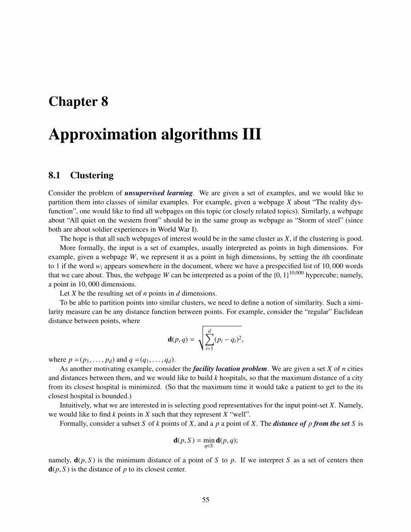
Chapter 8

Approximation algorithms III

8.1 Clustering

Consider the problem of unsupervised learning. We are given a set of examples, and we would like topartition them into classes of similar examples. For example, given a webpage X about “The reality dys-function”, one would like to find all webpages on this topic (or closely related topics). Similarly, a webpageabout “All quiet on the western front” should be in the same group as webpage as “Storm of steel” (sinceboth are about soldier experiences in World War I).

The hope is that all such webpages of interest would be in the same cluster as X, if the clustering is good.More formally, the input is a set of examples, usually interpreted as points in high dimensions. For

example, given a webpage W, we represent it as a point in high dimensions, by setting the ith coordinateto 1 if the word wi appears somewhere in the document, where we have a prespecified list of 10, 000 wordsthat we care about. Thus, the webpage W can be interpreted as a point of the 0, 110,000 hypercube; namely,a point in 10, 000 dimensions.

Let X be the resulting set of n points in d dimensions.To be able to partition points into similar clusters, we need to define a notion of similarity. Such a simi-

larity measure can be any distance function between points. For example, consider the “regular” Euclideandistance between points, where

d(p, q) =

√√√ d∑i=1

(pi − qi)2,

where p = (p1, . . . , pd) and q = (q1, . . . , qd).As another motivating example, consider the facility location problem. We are given a set X of n cities

and distances between them, and we would like to build k hospitals, so that the maximum distance of a cityfrom its closest hospital is minimized. (So that the maximum time it would take a patient to get to the itsclosest hospital is bounded.)

Intuitively, what we are interested in is selecting good representatives for the input point-set X. Namely,we would like to find k points in X such that they represent X “well”.

Formally, consider a subset S of k points of X, and a p a point of X. The distance of p from the set S is

d(p, S ) = minq∈S

d(p, q);

namely, d(p, S ) is the minimum distance of a point of S to p. If we interpret S as a set of centers thend(p, S ) is the distance of p to its closest center.

55

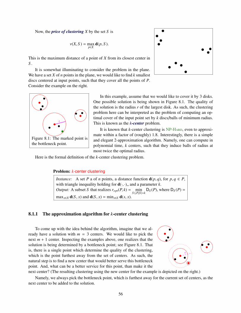
Now, the price of clustering X by the set S is

ν(X, S ) = maxp∈X

d(p, S ).

This is the maximum distance of a point of X from its closest center inS .

It is somewhat illuminating to consider the problem in the plane.We have a set X of n points in the plane, we would like to find k smallestdiscs centered at input points, such that they cover all the points of P.Consider the example on the right.

Figure 8.1: The marked point isthe bottleneck point.

In this example, assume that we would like to cover it by 3 disks.One possible solution is being shown in Figure 8.1. The quality ofthe solution is the radius r of the largest disk. As such, the clusteringproblem here can be interpreted as the problem of computing an op-timal cover of the input point set by k discs/balls of minimum radius.This is known as the k-center problem.

It is known that k-center clustering is NP-H, even to approxi-mate within a factor of (roughly) 1.8. Interestingly, there is a simpleand elegant 2-approximation algorithm. Namely, one can compute inpolynomial time, k centers, such that they induce balls of radius atmost twice the optimal radius.

Here is the formal definition of the k-center clustering problem.

Problem: k-center clustering

Instance: A set P a of n points, a distance function d(p, q), for p, q ∈ P,with triangle inequality holding for d(·, ·)„ and a parameter k.Output: A subset S that realizes ropt(P, k) = min

S⊆P,|S |=kDS (P), where DS (P) =

maxx∈X d(S , x) and d(S , x) = mins∈S d(s, x).

8.1.1 The approximation algorithm for k-center clustering

To come up with the idea behind the algorithm, imagine that we al-ready have a solution with m = 3 centers. We would like to pick thenext m + 1 center. Inspecting the examples above, one realizes that thesolution is being determined by a bottleneck point; see Figure 8.1. Thatis, there is a single point which determine the quality of the clustering,which is the point furthest away from the set of centers. As such, thenatural step is to find a new center that would better serve this bottleneckpoint. And, what can be a better service for this point, than make it thenext center? (The resulting clustering using the new center for the example is depicted on the right.)

Namely, we always pick the bottleneck point, which is furthest away for the current set of centers, as thenext center to be added to the solution.

56

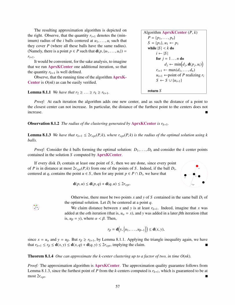
Algorithm AprxKCenter (P, k)P = p1, . . . , pn

S = p1, u1 ← p1while |S | < k do

i← |S |for j = 1 . . . n do

d j ← min(d j,d(p j, ui)

)ri+1 ← max(d1, . . . , dn)ui+1 ←point of P realizing ri

S ← S ∪ ui+1

return S

The resulting approximation algorithm is depicted onthe right. Observe, that the quantity ri+1 denotes the (min-imum) radius of the i balls centered at u1, . . . , ui such thatthey cover P (where all these balls have the same radius).(Namely, there is a point p ∈ P such that d(p, u!, . . . , ui) =ri+1.

It would be convenient, for the sake analysis, to imaginethat we run AprxKCenter one additional iteration, so thatthe quantity rk+1 is well defined.

Observe, that the running time of the algorithm AprxK-Center is O(nk) as can be easily verified.

Lemma 8.1.1 We have that r2 ≥ . . . ≥ rk ≥ rk+1.

Proof: At each iteration the algorithm adds one new center, and as such the distance of a point tothe closest center can not increase. In particular, the distance of the furthest point to the centers does notincrease.

Observation 8.1.2 The radius of the clustering generated by AprxKCenter is rk+1.

Lemma 8.1.3 We have that rk+1 ≤ 2ropt(P, k), where ropt(P, k) is the radius of the optimal solution using kballs.

Proof: Consider the k balls forming the optimal solution: D1, . . . ,Dk and consider the k center pointscontained in the solution S computed by AprxKCenter.

If every disk Di contain at least one point of S , then we are done, since every pointof P is in distance at most 2ropt(P, k) from one of the points of S . Indeed, if the ball Di,centered at q, contains the point u ∈ S , then for any point p ∈ P ∩ Di, we have that

d(p, u) ≤ d(p, q) + d(q, u) ≤ 2ropt.

q

ropt

x y

Otherwise, there must be two points x and y of S contained in the same ball Di ofthe optimal solution. Let Di be centered at a point q.

We claim distance between x and y is at least rk+1. Indeed, imagine that x wasadded at the αth iteration (that is, uα = x), and y was added in a later βth iteration (thatis, uβ = y), where α < β. Then,

rβ = d(y,

u1, . . . , uβ−1

)≤ d(x, y),

since x = uα and y = uβ. But rβ ≥ rk+1, by Lemma 8.1.1. Applying the triangle inequality again, we havethat rk+1 ≤ rβ ≤ d(x, y) ≤ d(x, q) + d(q, y) ≤ 2ropt, implying the claim.

Theorem 8.1.4 One can approximate the k-center clustering up to a factor of two, in time O(nk).

Proof: The approximation algorithm is AprxKCenter. The approximation quality guarantee follows fromLemma 8.1.3, since the furthest point of P from the k-centers computed is rk+1, which is guaranteed to be atmost 2ropt.

57

8.2 Subset SumProblem: Subset Sum

Instance: X = x1, . . . , xn – n integer positive numbers, t - target numberQuestion: Is there a subset of X such the sum of its elements is t?

SolveSubsetSum (X, t, M)b[0 . . . Mn] - boolean array initialized to FALSE.// b[x] is TRUE if x can be realized by a subset of X.

b[0]← TRUE.for i = 1, . . . , n do

for j = Mn down to xi dob[ j]← B[ j − xi] ∨ B[ j]

return B[t]

Subset Sum is (of course) NP-C,as we already proved. It can be solved inpolynomial time if the numbers of X are small.In particular, if xi ≤ M, for i = 1, . . . , n, thent ≤ Mn (otherwise, there is no solution). Itsreasonably easy to solve in this case, as thealgorithm on the right shows. The runningtime of the resulting algorithm is O(Mn2).

Note, that M my be prohibitly large, andas such, this algorithm is not polynomial inn. In particular, if M = 2n then this algorithm is prohibitly slow. Since the relevant decision problem isNPC, it is unlikely that an efficient algorithm exist for this problem. But still, we would like to be able tosolve it quickly and efficiently. So, if we want an efficient solution, we would have to change the problemslightly. As a first step, lets turn it into an optimization problem.

Problem: Subset Sum Optimization

Instance: (X, t): A set X of n positive integers, and a target number tOutput: The largest number γopt one can represent as a subset sum of Xwhich is smaller or equal to t

Intuitively, we would like to find a subset of X such that it sum is smaller than t but very close to t.Next, we turn problem into an approximation problem.

Problem: Subset Sum Approx

Instance: (X, t, ε): A set X of n positive integers, a target number t, andparameter ε > 0Output: A number z that one can represent as a subset sum of X, such that(1 − ε)γopt ≤ z ≤ γopt ≤ t.

The challenge is to solve this approximation problem efficiently. To demonstrate that there is hopethat can be done, consider the following simple approximation algorithm, that achieves a constant factorapproximation.

Lemma 8.2.1 If there is a subset sum that adds up to t one can find a subset sum that adds up to at leastγopt/2 in O(n log n) time.

Proof: Add the numbers from largest to smallest, whenever adding a number will make the sum exceed t,we throw it away. We claim that the generate sum γopt/2 ≤ s ≤ t. Clearly, if the total sum of the numbers issmaller than t, then no number is being rejected and s = γopt.

Otherwise, let u be the first number being reject, and let s′ be the partial subset sum, just before u isbeing rejected. Clearly, s′ > u > 0, s′ < t, and s′ + u > t. This implies t < s′ + u < s′ + s′ ≤ 2s′, whichimplies that s′ ≥ t/2. Namely, the subset sum output is larger than t/2.

58

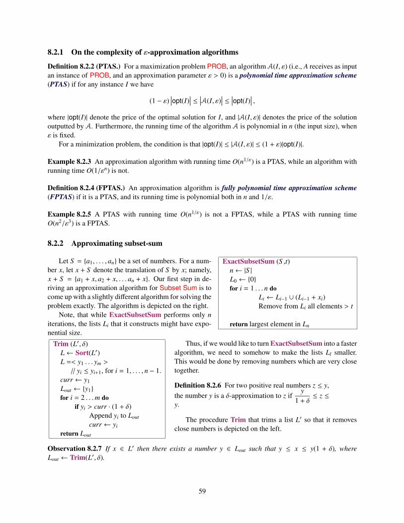
8.2.1 On the complexity of ε-approximation algorithms

Definition 8.2.2 (PTAS.) For a maximization problem PROB, an algorithm A(I, ε) (i.e., A receives as inputan instance of PROB, and an approximation parameter ε > 0) is a polynomial time approximation scheme(PTAS) if for any instance I we have

(1 − ε)∣∣∣opt(I)

∣∣∣ ≤ ∣∣∣A(I, ε)∣∣∣ ≤ ∣∣∣opt(I)

∣∣∣ ,where |opt(I)| denote the price of the optimal solution for I, and |A(I, ε)| denotes the price of the solutionoutputted by A. Furthermore, the running time of the algorithm A is polynomial in n (the input size), whenε is fixed.

For a minimization problem, the condition is that |opt(I)| ≤ |A(I, ε)| ≤ (1 + ε)|opt(I)|.

Example 8.2.3 An approximation algorithm with running time O(n1/ε) is a PTAS, while an algorithm withrunning time O(1/εn) is not.

Definition 8.2.4 (FPTAS.) An approximation algorithm is fully polynomial time approximation scheme(FPTAS) if it is a PTAS, and its running time is polynomial both in n and 1/ε.

Example 8.2.5 A PTAS with running time O(n1/ε) is not a FPTAS, while a PTAS with running timeO(n2/ε3) is a FPTAS.

8.2.2 Approximating subset-sum

ExactSubsetSum (S ,t)n← |S |L0 ← 0for i = 1 . . . n do

Li ← Li−1 ∪ (Li−1 + xi)Remove from Li all elements > t

return largest element in Ln

Let S = a1, . . . , an be a set of numbers. For a num-ber x, let x + S denote the translation of S by x; namely,x + S = a1 + x, a2 + x, . . . an + x. Our first step in de-riving an approximation algorithm for Subset Sum is tocome up with a slightly different algorithm for solving theproblem exactly. The algorithm is depicted on the right.

Note, that while ExactSubsetSum performs only niterations, the lists Li that it constructs might have expo-nential size.

Trim (L′, δ)L← Sort(L′)L =< y1 . . . ym >

// yi ≤ yi+1, for i = 1, . . . , n − 1.curr ← y1Lout ← y1

for i = 2 . . .m doif yi > curr · (1 + δ)

Append yi to Lout

curr ← yi

return Lout

Thus, if we would like to turn ExactSubsetSum into a fasteralgorithm, we need to somehow to make the lists Ll smaller.This would be done by removing numbers which are very closetogether.

Definition 8.2.6 For two positive real numbers z ≤ y,the number y is a δ-approximation to z if

y1 + δ

≤ z ≤y.

The procedure Trim that trims a list L′ so that it removesclose numbers is depicted on the left.

Observation 8.2.7 If x ∈ L′ then there exists a number y ∈ Lout such that y ≤ x ≤ y(1 + δ), whereLout ← Trim(L′, δ).

59

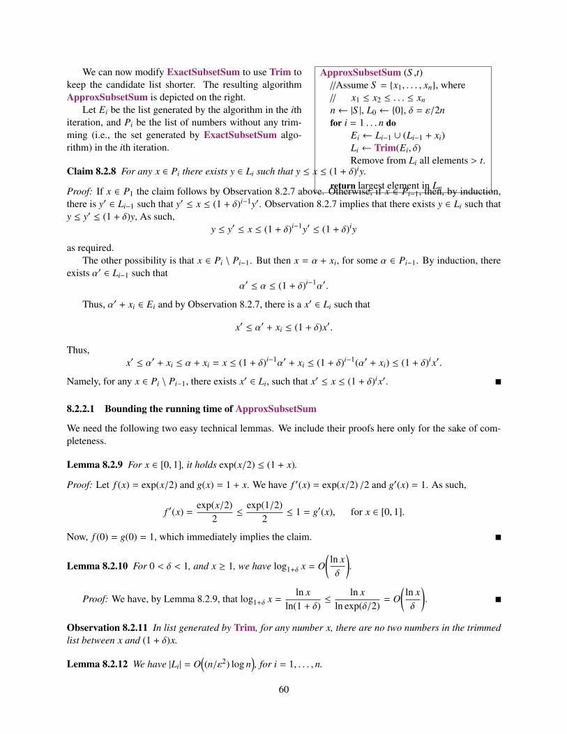
ApproxSubsetSum (S ,t)//Assume S = x1, . . . , xn, where// x1 ≤ x2 ≤ . . . ≤ xn

n← |S |, L0 ← 0, δ = ε/2nfor i = 1 . . . n do

Ei ← Li−1 ∪ (Li−1 + xi)Li ← Trim(Ei, δ)Remove from Li all elements > t.

return largest element in Ln

We can now modify ExactSubsetSum to use Trim tokeep the candidate list shorter. The resulting algorithmApproxSubsetSum is depicted on the right.

Let Ei be the list generated by the algorithm in the ithiteration, and Pi be the list of numbers without any trim-ming (i.e., the set generated by ExactSubsetSum algo-rithm) in the ith iteration.

Claim 8.2.8 For any x ∈ Pi there exists y ∈ Li such that y ≤ x ≤ (1 + δ)iy.

Proof: If x ∈ P1 the claim follows by Observation 8.2.7 above. Otherwise, if x ∈ Pi−1, then, by induction,there is y′ ∈ Li−1 such that y′ ≤ x ≤ (1 + δ)i−1y′. Observation 8.2.7 implies that there exists y ∈ Li such thaty ≤ y′ ≤ (1 + δ)y, As such,

y ≤ y′ ≤ x ≤ (1 + δ)i−1y′ ≤ (1 + δ)iy

as required.The other possibility is that x ∈ Pi \ Pi−1. But then x = α + xi, for some α ∈ Pi−1. By induction, there

exists α′ ∈ Li−1 such thatα′ ≤ α ≤ (1 + δ)i−1α′.

Thus, α′ + xi ∈ Ei and by Observation 8.2.7, there is a x′ ∈ Li such that

x′ ≤ α′ + xi ≤ (1 + δ)x′.

Thus,x′ ≤ α′ + xi ≤ α + xi = x ≤ (1 + δ)i−1α′ + xi ≤ (1 + δ)i−1(α′ + xi) ≤ (1 + δ)ix′.

Namely, for any x ∈ Pi \ Pi−1, there exists x′ ∈ Li, such that x′ ≤ x ≤ (1 + δ)ix′.

8.2.2.1 Bounding the running time of ApproxSubsetSum

We need the following two easy technical lemmas. We include their proofs here only for the sake of com-pleteness.

Lemma 8.2.9 For x ∈ [0, 1], it holds exp(x/2) ≤ (1 + x).

Proof: Let f (x) = exp(x/2) and g(x) = 1 + x. We have f ′(x) = exp(x/2) /2 and g′(x) = 1. As such,

f ′(x) =exp(x/2)

2≤

exp(1/2)2

≤ 1 = g′(x), for x ∈ [0, 1].

Now, f (0) = g(0) = 1, which immediately implies the claim.

Lemma 8.2.10 For 0 < δ < 1, and x ≥ 1, we have log1+δ x = O(ln xδ

).

Proof: We have, by Lemma 8.2.9, that log1+δ x =ln x

ln(1 + δ)≤

ln xln exp(δ/2)

= O(ln xδ

).

Observation 8.2.11 In list generated by Trim, for any number x, there are no two numbers in the trimmedlist between x and (1 + δ)x.

Lemma 8.2.12 We have |Li| = O((n/ε2) log n

), for i = 1, . . . , n.

60

Proof: The set Li−1 + xi is a set of numbers between xi and ixi, because xi is larger than x1 . . . xi−1 andLi−1 contains subset sums of at most i − 1 numbers, each one of them smaller than xi. As such, the numberof different values in this range, stored in the list Li, after trimming is at most

log1+δixi

xi= O

(ln iδ

)= O

(ln nδ

),

by Lemma 8.2.10. Thus,

|Li| ≤ |Li−1| + O(ln nδ

)≤ |Li−1| + O

(n ln nε

)= O

(n2 log n

ε

).

Lemma 8.2.13 The running time of ApproxSubsetSum is O(

n3

ε log n).

Proof: Clearly, the running time of ApproxSubsetSum is dominated by the total length of the lists L1, . . . , Ln

it creates. Lemma 8.2.12 implies that∑

i

|Li| = O(n3

εlog n

).

8.2.2.2 The result

Theorem 8.2.14 ApproxSubsetSum returns a number u ≤ t, such that

γopt

1 + ε≤ u ≤ γopt ≤ t,

where γopt is the optimal solution (i.e., largest realizable subset sum smaller than t).The running time of ApproxSubsetSum is O((n3/ε) ln n).

Proof: The running time bound is by Lemma 8.2.13.As for the other claim, consider the optimal solution opt ∈ Pn. By Claim 8.2.8, there exists z ∈ Ln such

that z ≤ opt ≤ (1 + δ)nz. However,

(1 + δ)n = (1 + ε/2n)n ≤ exp(ε

2

)≤ 1 + ε,

since 1 + x ≤ ex for x ≥ 0. Thus, opt/(1 + ε) ≤ z ≤ opt ≤ t, implying that the output of ApproxSubsetSumis within the required range.

8.3 Approximate Bin Packing

Consider the following problem.

Problem: Min Bin Packing

Instance: a1 . . . an – n numbers in [0, 1]Output: Q: What is the minimum number of unit bins do you need to use tostore all the numbers in S ?

Bin Packing is NP-C because you can reduce Partition to it. Its natural to ask how one canapproximate the optimal solution to Bin Packing.

One such algorithm is next fit. Here, we go over the numbers one by one, and put a number in thecurrent bin if that bin can contain it. Otherwise, we create a new bin and put the number in this bin. Clearly,we need at least

61

dAe bins where A =n∑

i=1

ai

Every two consecutive bins contain numbers that add up to more than 1, since otherwise we would have notcreated the second bin. As such, the number of bins used is 2 bAc. As such, the next fit algorithm for binpacking achieves a 2 approximation.

A better strategy, is to sort the numbers from largest to smallest and insert them in this order, where ineach stage, we scan all current bins, and see if can insert the current number into one of those bins. If wecan not, we create a new bin for this number. This is known as first fit. We state the approximation ratio forthis algorithm without proof.

Theorem 8.3.1 Decreasing first fit is a 1.5-approximation to Min Bin Packing.

8.4 Bibliographical notes

One can do 2-approximation for the k-center clustering in low dimensional Euclidean space can be done inΘ(n log k) time [FG88]. In fact, it can be solved in linear time [Har04].

62

Part II

Randomized Algorithms

63

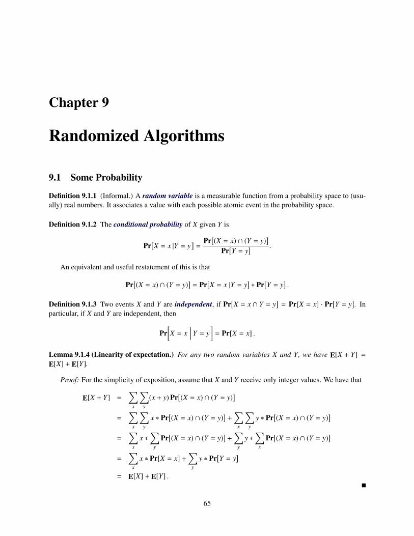
Chapter 9


9.1 Some Probability

Definition 9.1.1 (Informal.) A random variable is a measurable function from a probability space to (usu-ally) real numbers. It associates a value with each possible atomic event in the probability space.

Definition 9.1.2 The conditional probability of X given Y is

Pr[X = x |Y = y

]=

Pr[(X = x) ∩ (Y = y)

]Pr

[Y = y

] .

An equivalent and useful restatement of this is that

Pr[(X = x) ∩ (Y = y)

]= Pr

[X = x |Y = y

]∗ Pr

[Y = y

].

Definition 9.1.3 Two events X and Y are independent, if Pr[X = x ∩ Y = y

]= Pr[X = x] · Pr

[Y = y

]. In

particular, if X and Y are independent, then

Pr[X = x

∣∣∣∣ Y = y]= Pr[X = x] .

Lemma 9.1.4 (Linearity of expectation.) For any two random variables X and Y, we have E[X + Y] =E[X] + E[Y].

Proof: For the simplicity of exposition, assume that X and Y receive only integer values. We have that

E[X + Y] =∑

x

∑y

(x + y) Pr[(X = x) ∩ (Y = y)

]=

∑x

∑y

x ∗ Pr[(X = x) ∩ (Y = y)

]+

∑x

∑y

y ∗ Pr[(X = x) ∩ (Y = y)

]=

∑x

x ∗∑

y

Pr[(X = x) ∩ (Y = y)

]+

∑y

y ∗∑

x

Pr[(X = x) ∩ (Y = y)

]=

∑x

x ∗ Pr[X = x] +∑

y

y ∗ Pr[Y = y

]= E[X] + E[Y] .

65

9.2 Sorting Nuts and Bolts

Problem 9.2.1 (Sorting Nuts and Bolts) You are given a set of n nuts and n bolts. Every nut have amatching bolt, and all the n pairs of nuts and bolts have different sizes. Unfortunately, you get the nuts andbolts separated from each other and you have to match the nuts to the bolts. Furthermore, given a nut anda bolt, all you can do is to try and match one bolt against a nut (i.e., you can not compare two nuts to eachother, or two bolts to each other).

When comparing a nut to a bolt, either they match, or one is smaller than other (and you known therelationship after the comparison).

How to match the n nuts to the n bolts quickly? Namely, while performing a small number of compar-isons.

MatchNutsAndBolts(N: nuts, B: bolts)Pick a random nut npivot from NFind its matching bolt bpivot in BBL ← All bolts in B smaller than npivot

NL ← All nuts in N smaller than bpivot

BR ← All bolts in B larger than npivot

NR ← All nuts in N larger than bpivot

MatchNutsAndBolts(NR,BR)MatchNutsAndBolts(NL,BL)

The naive algorithm is of course to compare each nut toeach bolt, and match them together. This would require aquadratic number of comparisons. Another option is to sortthe nuts by size, and the bolts by size and then “merge” thetwo ordered sets, matching them by size. The only problem isthat we can not sorts only the nuts, or only the bolts, since wecan not compare them to each other. Indeed, we sort the twosets simultaneously, by simulating QuickSort. The resultingalgorithm is depicted on the right.

9.2.1 Running time analysis

Definition 9.2.2 Let RT denote the random variable which is the running time of the algorithm. Note, thatthe running time is a random variable as it might be different between different executions on the same input.

Definition 9.2.3 For a randomized algorithm, we can speak about the expected running time. Namely, weare interested in bounding the quantity E[RT] for the worst input.

Definition 9.2.4 The expected running-time of a randomized algorithm for input of size n is

T (n) = maxU is an input of size n

E[RT(U)

],

where RT(U) is the running time of the algorithm for the input U.

Definition 9.2.5 The rank of an element x in a set S , denoted by rank(x), is the number of elements in S ofsize smaller or equal to x. Namely, it is the location of x in the sorted list of the elements of S .

Theorem 9.2.6 The expected running time of MatchNutsAndBolts (and thus also of QuickSort) is T (n) =O(n log n), where n is the number of nuts and bolts. The worst case running time of this algorithm is O(n2).

Proof: Clearly, we have that Pr[rank(npivot) = k

]= 1

n . Furthermore, if the rank of the pivot is k then

T (n) = Ek=rank(npivot)[O(n) + T (k − 1) + T (n − k)] = O(n) + Ek[T (k − 1) + T (n − k)]

= T (n) = O(n) +n∑

k=1

Pr[Rank(Pivot) = k] ∗(T (k − 1) + T (n − k))

= O(n) +n∑

k=1

1n·(T (k − 1) + T (n − k)) ,

66

by the definition of expectation. It is not easy to verify that the solution to the recurrence T (n) = O(n) +∑nk=1

1n ·(T (k − 1) + T (n − k)) is O(n log n).

9.2.1.1 Alternative incorrect solution

The algorithm MatchNutsAndBolts is lucky if n4 ≤ rank(npivot) ≤ 3

4 n. Thus, Pr[“lucky”

]= 1/2. Intuitively,

for the algorithm to be fast, we want the split to be as balanced as possible. The less balanced the cut is, theworst the expected running time. As such, the “Worst” lucky position is when rank(npivot) = n/4 and wehave that

T (n) ≤ O(n) + Pr[“lucky”

]∗ (T (n/4) + T (3n/4)) + Pr

[“unlucky”

]∗ T (n).

Namely, T (n) = O(n)+ 12 ∗

(T ( n

4 ) + T ( 34 n)

)+ 1

2 T (n). Rewriting, we get the recurrence T (n) = O(n)+T (n/4)+T ((3/4)n), and its solution is O(n log n).

While this is a very intuitive and elegant solution that bounds the running time of QuickSort, it isalso incomplete. The interested reader should try and make this argument complete. After completion theargument is as involved as the previous argument. Nevertheless, this argumentation gives a good back of theenvelope analysis for randomized algorithms which can be applied in a lot of cases.

9.2.2 What are randomized algorithms?

Randomized algorithms are algorithms that use random numbers (retrieved usually from some unbiasedsource of randomness [say a library function that returns the result of a random coin flip]) to make decisionsduring the executions of the algorithm. The running time becomes a random variable. Analyzing the algo-rithm would now boil down to analyzing the behavior of the random variable RT(n), where n denotes thesize of the input.In particular, the expected running time E[RT(n)] is a quantity that we would be interestedin.

It is useful to compare the expected running time of a randomized algorithm, which is


E[RT(U)] ,

to the worst case running time of a deterministic (i.e., not randomized) algorithm, which is


RT(U),

FlipCoinswhile RandBit= 1 do

nothing;

Caveat Emptor:Note, that a randomized algorithm might have ex-ponential running time in the worst case (or even unbounded) while hav-ing good expected running time. For example, consider the algorithmFlipCoins depicted on the right. The expected running time of Flip-Coins is a geometric random variable with probability 1/2, as such we have that E

[RT( FlipCoins )

]= O(2).

However, FlipCoins can run forever if it always gets 1 from the RandBit function.This is of course a ludicrous argument. Indeed, the probability that FlipCoins runs for long decreases

very quickly as the number of steps increases. It can happen that it runs for long, but it is extremely unlikely.

Definition 9.2.7 The running time of a randomized algorithm Alg is O( f (n)) with high probability if

Pr[RT(Alg(n)) ≥ c · f (n)

]= o(1).

Caveat Emptor - let the buyer beware (i.e., one buys at one’s own risk)

67

Namely, the probability of the algorithm to take more than O( f (n)) time decreases to 0 as n goes to infinity.In our discussion, we would use the following (considerably more restrictive definition), that requires that

Pr[RT(Alg(n)) ≥ c · f (n)

]≤

1nd ,

where c and d are appropriate constants. For technical reasons, we also require that E[RT(Alg(n))

]=

O( f (n)).

9.3 Analyzing QuickSort

The previous analysis works also for QuickSort. However, there is an alternative analysis which is alsovery interesting and elegant. Let a1, ..., an be the n given numbers (in sorted order – as they appear in theoutput).

It is enough to bound the number of comparisons performed by QuickSort to bound its running time, ascan be easily verified. Observe, that two specific elements are compared to each other by QuickSort at mostonce, because QuickSort performs only comparisons against the pivot, and after the comparison happen,the pivot does not being passed to the two recursive subproblems.

Let Xi j be an indicator variable if QuickSort compared ai to a j in the current execution, and zerootherwise. The number of comparisons performed by QuickSort is exactly Z =

∑i< j Xi j.

Observation 9.3.1 The element ai is compared to a j iff one of them is picked to be the pivot and they arestill in the same subproblem.

Also, we have that µ = E[Xi j

]= Pr

[Xi j = 1

]. To quantify this probability, observe that if the pivot is

smaller than ai or larger than a j then the subproblem still contains the block of elements ai, . . . , a j. Thus,we have that

µ = Pr[ai or a j is first pivot ∈ ai, . . . , a j

]=

2j − i + 1

.

Another (and hopefully more intuitive) explanation for the above phenomena is the following: Imagine,that before running QuickSort we choose for every element a random priority, which is a real number inthe range [0, 1]. Now, we reimplement QuickSort such that it always pick the element with the lowestrandom priority (in the given subproblem) to be the pivot. One can verify that this variant and the standardimplementation have the same running time. Now, ai gets compares to a j if and only if all the elementsai+1, . . . , a j−1 have random priority larger than both the random priority of ai and the random priority of a j.But the probability that one of two elements would have the lowest random-priority out of j− i+ 1 elementsis 2 ∗ 1/( j − i + 1), as claimed.

Thus, the running time of QuickSort is

E[RT(n)

]= E

∑i< j

Xi j

=∑i< j

E[Xi j

]=

∑i< j

2j − i + 1

=∑∆= j−i+1

2n − ∆ + 1∆

≤ 2nn∑∆=2

1∆= 2nHn ≤ 2n(ln n + 1),

by linearity of expectations, where Hn ≤ ln n + 1 is the nth harmonic number,In fact, the running time of QuickSort is O(n log n) with high-probability. We need some more tools

before we can show that.

68

Chapter 10

Randomized Algorithms II

10.1 QuickSort with High Probability

One can think about QuickSort as playing a game in rounds. Every round, QuickSort picks a pivot, splitsthe problem into two subproblems, and continue playing the game recursively on both subproblems.

If we track a single element in the input, we see a sequence of rounds that involve this element. Thegame ends, when this element find itself alone in the round (i.e., the subproblem is to sort a single element).

Thus, to show that QuickSort takes O(n log n) time, it is enough to show, that every element in the input,participates in at most 32 ln n rounds with high enough probability.

Indeed, let Xi be the event that the ith element participates in more than 32 ln n rounds.Let CQS be the number of comparisons performed by QuickSort. A comparison between a pivot and an

element will be always charged to the element. And as such, the number of comparisons overall performedby QuickSort is bounded by

∑i ri, where ri is the number of rounds the ith element participated in (the last

round where it was a pivot is ignored). We have that

α = Pr[CQS ≥ 32n ln n

]≤ Pr

⋃i

Xi

≤ n∑i=1

Pr[Xi] .

Here, we used the union rule, that states that for any two events A and B, we have that Pr[A ∪ B] ≤Pr[A] + Pr[B]. Assume, for the time being, that Pr[Xi] ≤ 1/n3. This implies that

α ≤

n∑i=1

Pr[Xi] ≤n∑

i=1

1/n3 =1n2 .

Namely, QuickSort performs at most 32n ln n comparisons with high probability. It follows, that Quick-Sort runs in O(n log n) time, with high probability, since the running time of QuickSort is proportional tothe number of comparisons it performs.

To this end, we need to prove that Pr[Xi] ≤ 1/n3.

10.1.1 Proving that an elements participates in small number of rounds.

Consider a run of QuickSort for an input made out of n numbers. Consider a specific element x in thisinput, and let S 1, S 2, . . . be the subsets of the input that are in the recursive calls that include the elementx. Here S j is the set of numbers in the jth round (i.e., this is the recursive call at depth j which includes xamong the numbers it needs to sort).

69

The element x would be considered to be luckyQuick Sort!lucky, in the jth iteration, if the call tothe QuickSort, splits the current set S j into two parts, where both parts contains at most (3/4)

∣∣∣S j∣∣∣ of the

elements.Let Y j be an indicator variable which is 1 iff x is lucky in jth round. Formally, Y j = 1 iff

∣∣∣S j∣∣∣ /4 ≤∣∣∣S j+1

∣∣∣ ≤ 3∣∣∣S j

∣∣∣ /4. By definition, we have that

Pr[Y j

]=

12.

Furthermore, Y1,Y2, . . . ,Ym are all independent variables.Note, that x can participate in at most

ρ = log4/3 n ≤ 3.5 ln n (10.1)

rounds, since at each successful round, the number of elements in the subproblem shrinks by at least a factor3/4, and |S 1| = n. As such, if there are ρ successful rounds in the first k rounds, then |S k| ≤ (3/4)ρn ≤ 1.

Thus, the question of how many rounds x participates in, boils down to how many coin flips one need toperform till one gets ρ heads. Of course, in expectation, we need to do this 2ρ times. But what if we want abound that holds with high probability, how many rounds are needed then?

In the following, we require the following lemma, which we will prove in Section 10.2.

Lemma 10.1.1 In a sequence of M coin flips, the probability that the number of ones is smaller than L ≤M/4 is at most exp(−M/8).

To use Lemma 10.1.1, we setM = 32 ln n ≥ 8ρ,

see Eq. (10.1). Let Y j be the variable which is one if x is lucky in the jth level of recursion, and zerootherwise. We have that Pr

[Y j = 0

]= Pr

[Y j = 1

]= 1/2 and that Y1,Y2, . . . ,YM are independent. By

Lemma 10.1.1, we have that the probability that there are only ρ ≤ M/4 ones in Y1, . . . ,YM, is smaller than

exp(−

M8

)≤ exp(−ρ) ≤

1n3 .

We have that the probability that x participates in M recursive calls of QuickSort to be at most 1/n3.There are n input elements. Thus, the probability that depth of the recursion in QuickSort exceeds

32 ln n is smaller than (1/n3) ∗ n = 1/n2. We thus established the following result.

Theorem 10.1.2 With high probability (i.e., 1 − 1/n2) the depth of the recursion of QuickSort is ≤ 32 ln n.Thus, with high probability, the running time of QuickSort is O(n log n).

Of course, the same result holds for the algorithm MatchNutsAndBolts for matching nuts and bolts.

10.2 Chernoff inequality

10.2.1 Preliminaries

Theorem 10.2.1 (Markov’s Inequality.) For a non-negative variable X, and t > 0, we have:

Pr[X ≥ t] ≤ E[X]t

.

70

Proof: Assume that this is false, and there exists t0 > 0 such that Pr[X ≥ t0] > E[X]t0

. However,

E[X] =∑

x

x · Pr[X = x]

=∑x<t0

x · Pr[X = x] +∑x≥t0

x · Pr[X = x]

≥ 0 + t0 · Pr[X ≥ t0]

> 0 + t0 ·E[X]

t0= E[X] ,

a contradiction.We remind the reader that two random variables X and Y are independent if for any x, y we have that

Pr[(X = x) ∩ (Y = y)

]= Pr[X = x] · Pr

[Y = y

].

The following claim is easy to verify, and we omit the easy proof.

Claim 10.2.2 If X and Y are independent, then E[XY] = E[X] E[Y].If X and Y are independent then Z = eX and W = eY are also independent variables.

10.2.2 Chernoff inequality

Theorem 10.2.3 (Chernoff inequality.) Let X1, . . . , Xn be n independent random variables, such that Pr[Xi = 1] =Pr[Xi = −1] = 1

2 , for i = 1, . . . , n. Let Y =∑n

i=1 Xi. Then, for any ∆ > 0, we have

Pr[Y ≥ ∆] ≤ exp(−∆2/2n

).

Proof: Clearly, for an arbitrary t, to be specified shortly, we have

Pr[Y ≥ ∆] = Pr[tY ≥ t∆

]= Pr

[exp(tY) ≥ exp(t∆)

]≤

E[

exp(tY)]

exp(t∆), (10.2)

where the first part follows since exp(·) preserve ordering, and the second part follows by Markov’s inequal-ity (Theorem 10.2.1).

Observe that, by the definition of E[·] and by the Taylor expansion of exp(·), we have

E[

exp(tXi)]=

12

et +12

e−t =et + e−t

2

=12

(1 +

t1!+

t2

2!+

t3

3!+ · · ·

)+

12

(1 −

t1!+

t2

2!−

t3

3!+ · · ·

)=

(1 + +

t2

2!+ + · · · +

t2k

(2k)!+ · · ·

).

Now, (2k)! = k!(k + 1)(k + 2) · · · 2k ≥ k!2k, and thus

E[exp(tXi)

]=

∞∑i=0

t2i

(2i)!≤

∞∑i=0

t2i

2i(i!)=

∞∑i=0

1i!

(t2

2

)i

= exp(t2

2

),

71

again, by the Taylor expansion of exp(·). Next, by the independence of the Xis, we have

E[exp(tY)

]= E

exp

∑i

tXi

= E

∏i

exp(tXi)

= n∏i=1

E[exp(tXi)

]≤

n∏i=1

exp(t2

2

)= exp

(nt2

2

).

We have, by Eq. (10.2), that

Pr[Y ≥ ∆] ≤E[

exp(tY)]

exp(t∆)≤

exp(

nt22

)exp(t∆)

= exp(nt2

2− t∆

).

Next, we select the value of t that minimizes the right term in the above inequality. Easy calculation showsthat the right value is t = ∆/n. We conclude that

Pr[Y ≥ ∆] ≤ exp

n2

(∆

n

)2

−∆

n∆

= exp(−∆2

2n

).

Note, the above theorem states is that

Pr[Y ≥ ∆] =n∑

i=∆

Pr[Y = i] =n∑

i=n/2+∆/2

(ni

)2n ≤ exp

(−∆2

2n

),

since Y = ∆ means that we got n/2 + ∆/2 times +1s and n/2 − ∆/2 times (−1)s.By the symmetry of Y , we get the following corollary.

Corollary 10.2.4 Let X1, . . . , Xn be n independent random variables, such that Pr[Xi = 1] = Pr[Xi = −1] =12 , for i = 1, . . . , n. Let Y =

∑ni=1 Xi. Then, for any ∆ > 0, we have

Pr[|Y | ≥ ∆] ≤ 2 exp(−∆2

2n

).

By easy manipulation, we get the following result.

Corollary 10.2.5 Let X1, . . . , Xn be n independent coin flips, such that Pr[Xi = 1] = Pr[Xi = 0] = 12 , for

i = 1, . . . , n. Let Y =∑n

i=1 Xi. Then, for any ∆ > 0, we have

Pr[ n

2− Y ≥ ∆

]≤ exp

(−

2∆2

n

)and Pr

[Y −

n2≥ ∆

]≤ exp

(−

2∆2

n

).

In particular, we have Pr[∣∣∣∣∣Y − n

2

∣∣∣∣∣ ≥ ∆] ≤ 2 exp(−

2∆2

n

).

Proof: Transform Xi into the random variable Zi = 2Xi − 1, and now use Theorem 10.2.3 on the newrandom variables Z1, . . . ,Zn.

Lemma 10.1.1 (Restatement.) In a sequence of M coin flips, the probability that the number of ones issmaller than L ≤ M/4 is at most exp(−M/8).

Proof: Let Y =∑m

i=1 Xi the sum of the M coin flips. By the above corollary, we have:

Pr[Y ≤ L] = Pr[ M

2− Y ≥

M2− L

]= Pr

[ M2− Y ≥ ∆

],

where ∆ = M/2 − L ≥ M/4. Using the above Chernoff inequality, we get

Pr[Y ≤ L] ≤ exp(−

2∆2

M

)≤ exp(−M/8).

72

10.2.2.1 The Chernoff Bound — General Case

Here we present the Chernoff bound in a more general settings.

Problem 10.2.6 Let X1, . . . Xn be n independent Bernoulli trials, where

Pr[Xi = 1] = pi and Pr[Xi = 0] = 1 − pi

Y =∑

i

Xi µ = E[Y] .

Question: what is the probability that Y ≥ (1 + δ)µ.

Theorem 10.2.7 (Chernoff inequality) For any δ > 0,

Pr[Y > (1 + δ)µ

]<

(eδ

(1 + δ)1+δ

)µ.

Or in a more simplified form, for any δ ≤ 2e − 1,

Pr[Y > (1 + δ)µ

]< exp

(−µδ2/4

), (10.3)

andPr

[Y > (1 + δ)µ

]< 2−µ(1+δ),

for δ ≥ 2e − 1.

Theorem 10.2.8 Under the same assumptions as the theorem above, we have

Pr[Y < (1 − δ)µ

]≤ exp

(−µ

δ2

2

).

The proofs of those more general form, follows the proofs shown above, and are omitted. The interestedreader can get the proofs from:

http://www.uiuc.edu/~sariel/teach/2002/a/notes/07_chernoff.ps

73

http://www.uiuc.edu/~sariel/teach/2002/a/notes/07_chernoff.ps

74

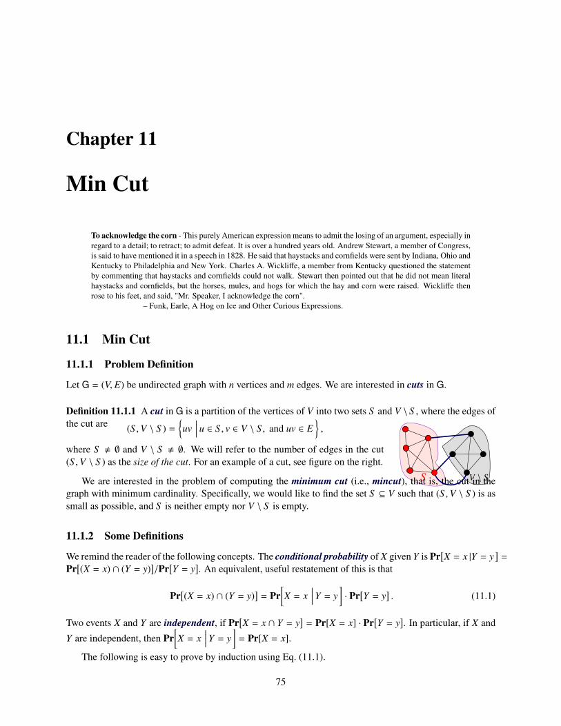
Chapter 11

Min Cut

To acknowledge the corn - This purely American expression means to admit the losing of an argument, especially inregard to a detail; to retract; to admit defeat. It is over a hundred years old. Andrew Stewart, a member of Congress,is said to have mentioned it in a speech in 1828. He said that haystacks and cornfields were sent by Indiana, Ohio andKentucky to Philadelphia and New York. Charles A. Wickliffe, a member from Kentucky questioned the statementby commenting that haystacks and cornfields could not walk. Stewart then pointed out that he did not mean literalhaystacks and cornfields, but the horses, mules, and hogs for which the hay and corn were raised. Wickliffe thenrose to his feet, and said, "Mr. Speaker, I acknowledge the corn".

– Funk, Earle, A Hog on Ice and Other Curious Expressions.

11.1 Min Cut

11.1.1 Problem Definition

Let G = (V, E) be undirected graph with n vertices and m edges. We are interested in cuts in G.

Definition 11.1.1 A cut in G is a partition of the vertices of V into two sets S and V \ S , where the edges ofthe cut are

V \ SS

(S ,V \ S ) =uv

∣∣∣∣ u ∈ S , v ∈ V \ S , and uv ∈ E,

where S , ∅ and V \ S , ∅. We will refer to the number of edges in the cut(S ,V \ S ) as the size of the cut. For an example of a cut, see figure on the right.

We are interested in the problem of computing the minimum cut (i.e., mincut), that is, the cut in thegraph with minimum cardinality. Specifically, we would like to find the set S ⊆ V such that (S ,V \ S ) is assmall as possible, and S is neither empty nor V \ S is empty.

11.1.2 Some Definitions

We remind the reader of the following concepts. The conditional probability of X given Y is Pr[X = x |Y = y

]=

Pr[(X = x) ∩ (Y = y)

]/Pr

[Y = y

]. An equivalent, useful restatement of this is that

Pr[(X = x) ∩ (Y = y)

]= Pr

[X = x

∣∣∣∣ Y = y]· Pr

[Y = y

]. (11.1)

Two events X and Y are independent, if Pr[X = x ∩ Y = y

]= Pr[X = x] · Pr

[Y = y

]. In particular, if X and

Y are independent, then Pr[X = x

∣∣∣∣ Y = y]= Pr[X = x].

The following is easy to prove by induction using Eq. (11.1).

75

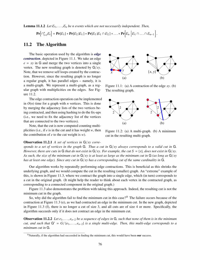
Lemma 11.1.2 Let E1, . . . ,En be n events which are not necessarily independent. Then,

Pr[∩n

i=1Ei]= Pr[E1] ∗ Pr[E2 |E1 ] ∗ Pr[E3 |E1 ∩ E2 ] ∗ . . . ∗ Pr

[En

∣∣∣∣E1 ∩ . . . ∩ En−1

].

11.2 The Algorithm

x y x, y

(a) (b)

Figure 11.1: (a) A contraction of the edge xy. (b)The resulting graph.

The basic operation used by the algorithm is edgecontraction, depicted in Figure 11.1. We take an edgee = xy in G and merge the two vertices into a singlevertex. The new resulting graph is denoted by G/xy.Note, that we remove self loops created by the contrac-tion. However, since the resulting graph is no longera regular graph, it has parallel edges – namely, it isa multi-graph. We represent a multi-graph, as a reg-ular graph with multiplicities on the edges. See Fig-ure 11.2.

22

22

(a) (b)

Figure 11.2: (a) A multi-graph. (b) A minimumcut in the resulting multi-graph.

The edge contraction operation can be implementedin O(n) time for a graph with n vertices. This is doneby merging the adjacency lists of the two vertices be-ing contracted, and then using hashing to do the fix-ups(i.e., we need to fix the adjacency list of the verticesthat are connected to the two vertices).

Note, that the cut is now computed counting multi-plicities (i.e., if e is in the cut and it has weight w, thenthe contribution of e to the cut weight is w).

Observation 11.2.1 A set of vertices in G/xy corre-sponds to a set of vertices in the graph G. Thus a cut in G/xy always corresponds to a valid cut in G.However, there are cuts in G that do not exist in G/xy. For example, the cut S = x, does not exist in G/xy.As such, the size of the minimum cut in G/xy is at least as large as the minimum cut in G (as long as G/xyhas at least one edge). Since any cut in G/xy has a corresponding cut of the same cardinality in G.

Our algorithm works by repeatedly performing edge contractions. This is beneficial as this shrinks theunderlying graph, and we would compute the cut in the resulting (smaller) graph. An “extreme” example ofthis, is shown in Figure 11.3, where we contract the graph into a single edge, which (in turn) corresponds toa cut in the original graph. (It might help the reader to think about each vertex in the contracted graph, ascorresponding to a connected component in the original graph.)

Figure 11.3 also demonstrates the problem with taking this approach. Indeed, the resulting cut is not theminimum cut in the graph.

So, why did the algorithm fail to find the minimum cut in this case? The failure occurs because of thecontraction at Figure 11.3 (e), as we had contracted an edge in the minimum cut. In the new graph, depictedin Figure 11.3 (f), there is no longer a cut of size 3, and all cuts are of size 4 or more. Specifically, thealgorithm succeeds only if it does not contract an edge in the minimum cut.

Observation 11.2.2 Let e1, . . . , en−2 be a sequence of edges in G, such that none of them is in the minimumcut, and such that G′ = G/ e1, . . . , en−2 is a single multi-edge. Then, this multi-edge corresponds to aminimum cut in G.

Naturally, if the algorithm had succeeded in finding the minimum cut, this would have been our success.

76

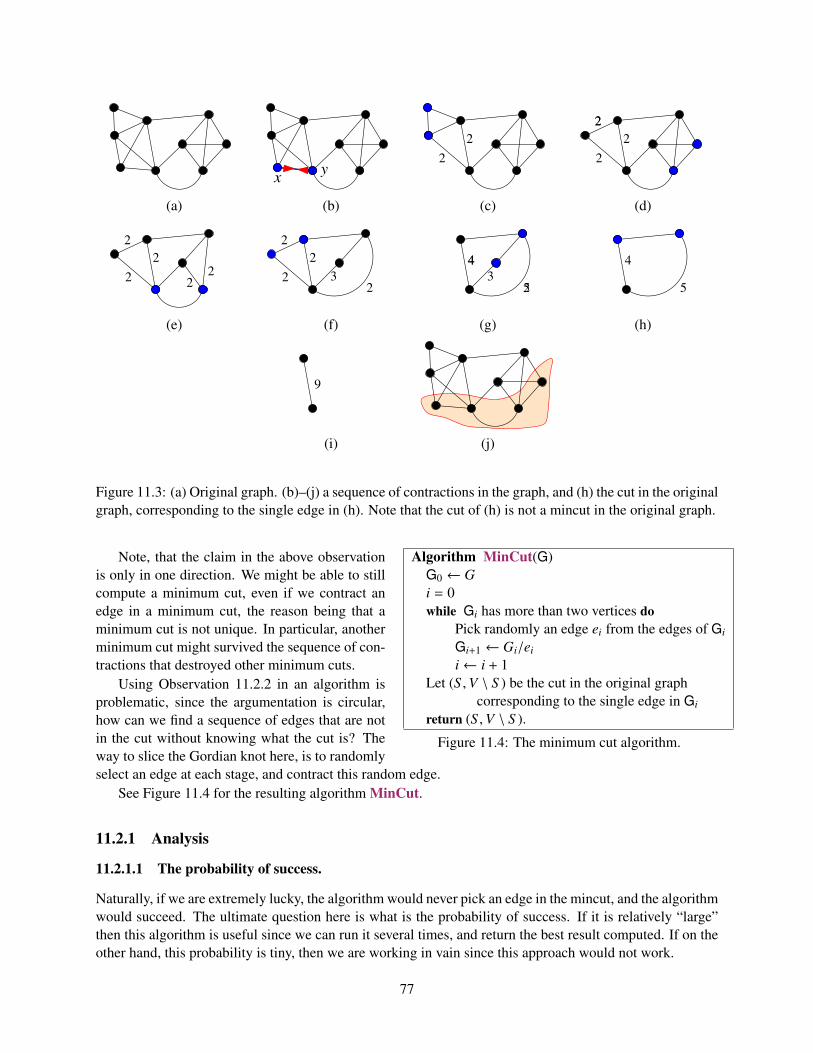
x y2

22

222

(a) (b) (c) (d)

22

2

22 2

22

23

23

44

5

4

5

(e) (f) (g) (h)

9

(i) (j)

Figure 11.3: (a) Original graph. (b)–(j) a sequence of contractions in the graph, and (h) the cut in the originalgraph, corresponding to the single edge in (h). Note that the cut of (h) is not a mincut in the original graph.

Algorithm MinCut(G)G0 ← Gi = 0while Gi has more than two vertices do

Pick randomly an edge ei from the edges of Gi

Gi+1 ← Gi/ei

i← i + 1Let (S ,V \ S ) be the cut in the original graph

corresponding to the single edge in Gi

return (S ,V \ S ).

Figure 11.4: The minimum cut algorithm.

Note, that the claim in the above observationis only in one direction. We might be able to stillcompute a minimum cut, even if we contract anedge in a minimum cut, the reason being that aminimum cut is not unique. In particular, anotherminimum cut might survived the sequence of con-tractions that destroyed other minimum cuts.

Using Observation 11.2.2 in an algorithm isproblematic, since the argumentation is circular,how can we find a sequence of edges that are notin the cut without knowing what the cut is? Theway to slice the Gordian knot here, is to randomlyselect an edge at each stage, and contract this random edge.

See Figure 11.4 for the resulting algorithm MinCut.

11.2.1 Analysis

11.2.1.1 The probability of success.

Naturally, if we are extremely lucky, the algorithm would never pick an edge in the mincut, and the algorithmwould succeed. The ultimate question here is what is the probability of success. If it is relatively “large”then this algorithm is useful since we can run it several times, and return the best result computed. If on theother hand, this probability is tiny, then we are working in vain since this approach would not work.

77

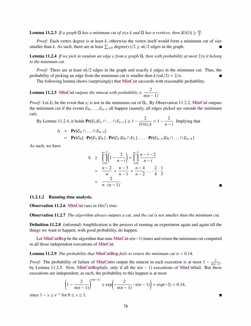
Lemma 11.2.3 If a graph G has a minimum cut of size k and G has n vertices, then |E(G)| ≥ kn2 .

Proof: Each vertex degree is at least k, otherwise the vertex itself would form a minimum cut of sizesmaller than k. As such, there are at least

∑v∈V degree(v)/2 ≥ nk/2 edges in the graph.

Lemma 11.2.4 If we pick in random an edge e from a graph G, then with probability at most 2/n it belongto the minimum cut.

Proof: There are at least nk/2 edges in the graph and exactly k edges in the minimum cut. Thus, theprobability of picking an edge from the minimum cut is smaller then k/(nk/2) = 2/n.

The following lemma shows (surprisingly) that MinCut succeeds with reasonable probability.

Lemma 11.2.5 MinCut outputs the mincut with probability ≥2

n(n − 1).

Proof: Let Ei be the event that ei is not in the minimum cut of Gi. By Observation 11.2.2, MinCut outputsthe minimum cut if the events E0, . . . ,En−3 all happen (namely, all edges picked are outside the minimumcut).

By Lemma 11.2.4, it holds Pr[Ei |E1 ∩ . . . ∩ Ei−1 ] ≥ 1 −2

|V(Gi)|= 1 −

2n − i

. Implying that

∆ = Pr[E0 ∩ . . . ∩ En−2]

= Pr[E0] · Pr[E1 |E0 ] · Pr[E2 |E0 ∩ E1 ] · . . . · Pr[En−3 |E0 ∩ . . . ∩ En−4 ]

As such, we have

∆ ≥

n−3∏i=0

(1 −

2n − i

)=

n−3∏i=0

n − i − 2n − i

=n − 2

n∗

n − 3n − 1

∗n − 4n − 2

. . . ·24·

13

=2

n · (n − 1).

11.2.1.2 Running time analysis.

Observation 11.2.6 MinCut runs in O(n2) time.

Observation 11.2.7 The algorithm always outputs a cut, and the cut is not smaller than the minimum cut.

Definition 11.2.8 (informal) Amplification is the process of running an experiment again and again till thethings we want to happen, with good probability, do happen.

Let MinCutRep be the algorithm that runs MinCut n(n−1) times and return the minimum cut computedin all those independent executions of MinCut.

Lemma 11.2.9 The probability that MinCutRep fails to return the minimum cut is < 0.14.

Proof: The probability of failure of MinCutto output the mincut in each execution is at most 1 − 2n(n−1) ,

by Lemma 11.2.5. Now, MinCutRepfails, only if all the n(n − 1) executions of MinCutfail. But theseexecutions are independent, as such, the probability to this happen is at most(

1 −2

n(n − 1)

)n(n−1)

≤ exp(−

2n(n − 1)

· n(n − 1))= exp(−2) < 0.14,

since 1 − x ≤ e−x for 0 ≤ x ≤ 1.

78

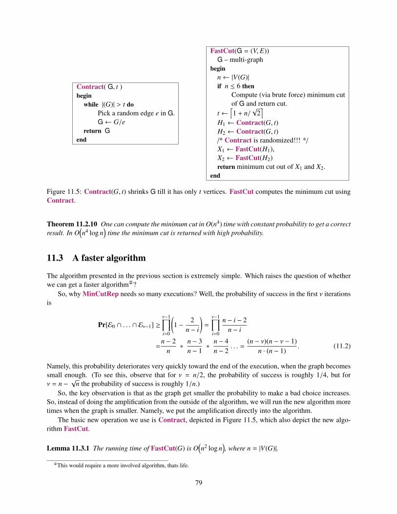
Contract( G, t )begin

while |(G)| > t doPick a random edge e in G.G← G/e

return Gend

FastCut(G = (V, E))G – multi-graph

beginn← |V(G)|if n ≤ 6 then

Compute (via brute force) minimum cutof G and return cut.

t ←⌈1 + n/

√2⌉

H1 ← Contract(G, t)H2 ← Contract(G, t)/* Contract is randomized!!! */X1 ← FastCut(H1),X2 ← FastCut(H2)return minimum cut out of X1 and X2.

end

Figure 11.5: Contract(G, t) shrinks G till it has only t vertices. FastCut computes the minimum cut usingContract.

Theorem 11.2.10 One can compute the minimum cut in O(n4) time with constant probability to get a correctresult. In O

(n4 log n

)time the minimum cut is returned with high probability.

11.3 A faster algorithm

The algorithm presented in the previous section is extremely simple. Which raises the question of whetherwe can get a faster algorithm?

So, why MinCutRep needs so many executions? Well, the probability of success in the first ν iterationsis

Pr[E0 ∩ . . . ∩ Eν−1] ≥ν−1∏i=0

(1 −

2n − i

)=

ν−1∏i=0

n − i − 2n − i

=n − 2

n∗

n − 3n − 1

∗n − 4n − 2

. . . =(n − ν)(n − ν − 1)

n · (n − 1). (11.2)

Namely, this probability deteriorates very quickly toward the end of the execution, when the graph becomessmall enough. (To see this, observe that for ν = n/2, the probability of success is roughly 1/4, but forν = n −

√n the probability of success is roughly 1/n.)

So, the key observation is that as the graph get smaller the probability to make a bad choice increases.So, instead of doing the amplification from the outside of the algorithm, we will run the new algorithm moretimes when the graph is smaller. Namely, we put the amplification directly into the algorithm.

The basic new operation we use is Contract, depicted in Figure 11.5, which also depict the new algo-rithm FastCut.

Lemma 11.3.1 The running time of FastCut(G) is O(n2 log n

), where n = |V(G)|.

This would require a more involved algorithm, thats life.

79

Proof: Well, we perform two calls to Contract(G, t) which takes O(n2) time. And then we perform tworecursive calls on the resulting graphs. We have:

T (n) = O(n2

)+ 2T

(n√

2

)The solution to this recurrence is O

(n2 log n

)as one can easily (and should) verify.

Exercise 11.3.2 Show that one can modify FastCut so that it uses only O(n2) space.

Lemma 11.3.3 The probability that Contract(G, n/√

2) had not contracted the minimum cut is at least 1/2.Namely, the probability that the minimum cut in the contracted graph is still a minimum cut in the

original graph is at least 1/2.

Proof: Just plug in ν = n − t = n −⌈1 + n/

√2⌉

into Eq. (11.2). We have

Pr[E0 ∩ . . . ∩ En−t] ≥t(t − 1)

n · (n − 1)=

⌈1 + n/

√2⌉(⌈

1 + n/√

2⌉− 1

)n(n − 1)

≥12.

The following lemma bounds the probability of success.

Lemma 11.3.4 FastCut finds the minimum cut with probability larger than Ω(1/ log n

).

Proof: Let P(n) be the probability that the algorithm succeeds on a graph with n vertices.The probability to succeed in the first call on H1 is the probability that Contract did not hit the minimum

cut (this probability is larger than 1/2 by Lemma 11.3.3), times the probability that the algorithm succeededon H1 in the recursive call (those two events are independent). Thus, the probability to succeed on the call

on H1 is at least (1/2) ∗ P(n/√

2), Thus, the probability to fail on H1 is ≤ 1 − 12 P

(n√2

).

The probability to fail on both H1 and H2 is smaller than(1 −

12

P(

n√

2

))2

,

since H1 and H2 are being computed independently. Note that if the algorithm, say, fails on H1 but succeedson H2 then it succeeds to return the mincut. Thus the above expression bounds the probability of failure.And thus, the probability for the algorithm to succeed is

P(n) ≥ 1 −(1 −

12

P(

n√

2

))2

= P(

n√

2

)−

14

(P(

n√

2

))2

.

We need to solve this recurrence. (This is very tedious, but since the details are non-trivial we providethe details of how to do so.) Divide both sides of the equation by P

(n/√

2)

we have:

P(n)

P(n/√

2)≥ 1 −

14

P(n/√

2).

It is now easy to verify that this inequality holds for P(n) ≥ c/ log n (since the worst case is P(n) =c/ log n we verify this inequality for this value). Indeed,

c/ log n

c/ log(n/√

2)≥ 1 −

c

4 log(n/√

2).

80

As such, letting ∆ = log n, we have

log n − log√

2log n

=∆ − log

√2

∆≥

4(log n − log√

2) − c

4(log n − log√

2)=

4(∆ − log√

2) − c

4(∆ − log√

2).

Equivalently, 4(∆−log√

2)2 ≥ 4∆(∆−log√

2)−c∆. Which implies −8∆ log√

2+4 log2√

2 ≥ −4∆ log√

2−c∆. Namely,

c∆ − 4∆ log√

2 + 4 log2√

2 ≥ 0,

which clearly holds for c ≥ 4 log√

2.We conclude, that the algorithm succeeds in finding the minimum cut in probability

≥ 2 log 2/ log n.

(Note that the base of the induction holds because we use brute force, and then P(i) = 1 for small i.)

Exercise 11.3.5 Prove, that running FastCut repeatedly c·log2 n times, guarantee that the algorithm outputsthe minimum cut with probability ≥ 1 − 1/n2, say, for c a constant large enough.

Theorem 11.3.6 One can compute the minimum cut in a graph G with n vertices in O(n2 log3 n) time. Thealgorithm succeeds with probability ≥ 1 − 1/n2.

Proof: We do amplification on FastCutby running it O(log2 n) times. The running time bound followsfrom Lemma 11.3.1. The bound on the probability follows from Lemma 11.3.4, and using the amplificationanalysis as done in Lemma 11.2.9 for MinCutRep.


The MinCut algorithm was developed by David Karger during his PhD thesis in Stanford. The fast algo-rithm is a joint work with Clifford Stein. The basic algorithm of the mincut is described in [MR95, pages7–9], the faster algorithm is described in [MR95, pages 289–295].

81

82

Part III

Network Flow

83

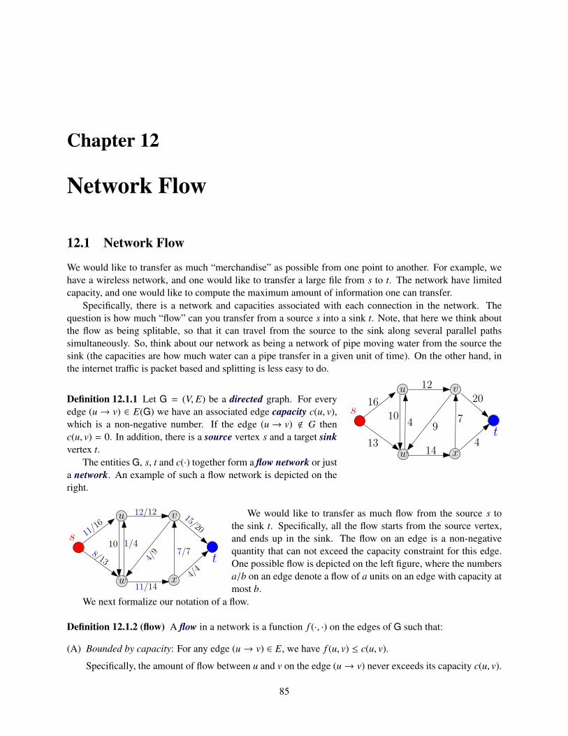
Chapter 12

Network Flow

12.1 Network Flow

We would like to transfer as much “merchandise” as possible from one point to another. For example, wehave a wireless network, and one would like to transfer a large file from s to t. The network have limitedcapacity, and one would like to compute the maximum amount of information one can transfer.

Specifically, there is a network and capacities associated with each connection in the network. Thequestion is how much “flow” can you transfer from a source s into a sink t. Note, that here we think aboutthe flow as being splitable, so that it can travel from the source to the sink along several parallel pathssimultaneously. So, think about our network as being a network of pipe moving water from the source thesink (the capacities are how much water can a pipe transfer in a given unit of time). On the other hand, inthe internet traffic is packet based and splitting is less easy to do.

s

13

410

14

t7

4

1220

9

16u v

w x

Definition 12.1.1 Let G = (V, E) be a directed graph. For everyedge (u→ v) ∈ E(G) we have an associated edge capacity c(u, v),which is a non-negative number. If the edge (u→ v) < G thenc(u, v) = 0. In addition, there is a source vertex s and a target sinkvertex t.

The entities G, s, t and c(·) together form a flow network or justa network. An example of such a flow network is depicted on theright.

s 11/1

6

t10

8/13

1/4

4/9 7/7

15/20

12/12

4/4

11/14

u v

w x

We would like to transfer as much flow from the source s tothe sink t. Specifically, all the flow starts from the source vertex,and ends up in the sink. The flow on an edge is a non-negativequantity that can not exceed the capacity constraint for this edge.One possible flow is depicted on the left figure, where the numbersa/b on an edge denote a flow of a units on an edge with capacity atmost b.

We next formalize our notation of a flow.

Definition 12.1.2 (flow) A flow in a network is a function f (·, ·) on the edges of G such that:

(A) Bounded by capacity: For any edge (u→ v) ∈ E, we have f (u, v) ≤ c(u, v).

Specifically, the amount of flow between u and v on the edge (u→ v) never exceeds its capacity c(u, v).

85

(B) Anti symmetry: For any u, v we have f (u, v) = − f (v, u).

(C) There are two special vertices: (i) the source vertex s (all flow starts from the source), and the sinkvertex t (all the flow ends in the sink).

(D) Conservation of flow: For any vertex u ∈ V \ s, t, we have∑

v

f (u, v) = 0.®

(Namely, for any internal node, all the flow that flows into a vertex leaves this vertex.)

The amount of flow (or just flow) of f , called the value of f , is | f | =∑v∈V

f (s, v).

Note, that a flow on edge can be negative (i.e., there is a positive flow flowing on this edge in the otherdirection).

Problem 12.1.3 (Maximum flow.) Given a network G find the maximum flow in G. Namely, compute alegal flow f such that | f | is maximized.

12.2 Some properties of flows, max flows, and residual networks

For two sets X,Y ⊆ V , let f (X,Y) =∑

x∈X,y∈Y f (x, y). We will slightly abuse the notations and refer tof(v , S

)by f (v, S ), where v ∈ V(G).

Observation 12.2.1 | f | = f (s,V).

Lemma 12.2.2 For a flow f , the following properties holds:

(i) ∀u ∈ V(G) we have f (u, u) = 0,

(ii) ∀X ⊆ V we have f (X, X) = 0,

(iii) ∀X,Y ⊆ V we have f (X,Y) = − f (Y, X),

(iv) ∀X,Y,Z ⊆ V such that X ∩ Y = ∅ we have that f (X ∪ Y,Z) = f (X,Z) + f (Y,Z) and f (Z, X ∪ Y) =f (Z, X) + f (Z,Y).

(v) For all u ∈ V \ s, t, we have f (u,V) = f (V, u) = 0.

Proof: Property (i) holds since (u→ u) it not an edge in the graph, and as such its flow is zero. As forproperty (ii), we have

f (X, X) =∑

u,v⊆X,u,v

( f (u, v) + f (v, u)) +∑u∈X

f (u, u) =∑

u,v⊆X,u,v

( f (u, v) − f (u, v)) +∑u∈X

0 = 0,

by the anti-symmetry property of flow (Definition 12.1.2 (B)).Property (iii) holds immediately by the anti-symmetry of flow, as f (X,Y) =

∑x∈X,y∈Y f (x, y) = −

∑x∈X,y∈Y f (y, x) =

− f (Y, X).(iv) This case follows immediately from definition.Finally (v) is just a restatement of the conservation of flow property.

Claim 12.2.3 | f | = f (V, t).®This law for electric circuits is known as Kirchhoff’s Current Law.

86

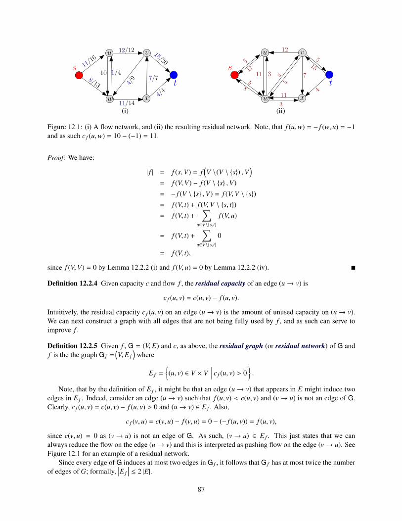
s 11/1

6

t10

8/13

1/4

4/9 7/7

15/20

12/12

4/4

11/14

u v

w x

s

t

u v

w x

5

115

3

5

7

5

12

4

3

11

8

4

11

15

(i) (ii)

Figure 12.1: (i) A flow network, and (ii) the resulting residual network. Note, that f (u,w) = − f (w, u) = −1and as such c f (u,w) = 10 − (−1) = 11.

Proof: We have:

| f | = f (s,V) = f(V \(V \ s) ,V

)= f (V,V) − f (V \ s ,V)

= − f (V \ s ,V) = f (V,V \ s)

= f (V, t) + f (V,V \ s, t)

= f (V, t) +∑

u∈V\s,t

f (V, u)

= f (V, t) +∑

u∈V\s,t

0

= f (V, t),

since f (V,V) = 0 by Lemma 12.2.2 (i) and f (V, u) = 0 by Lemma 12.2.2 (iv).

Definition 12.2.4 Given capacity c and flow f , the residual capacity of an edge (u→ v) is

c f (u, v) = c(u, v) − f (u, v).

Intuitively, the residual capacity c f (u, v) on an edge (u→ v) is the amount of unused capacity on (u→ v).We can next construct a graph with all edges that are not being fully used by f , and as such can serve toimprove f .

Definition 12.2.5 Given f , G = (V, E) and c, as above, the residual graph (or residual network) of G andf is the the graph G f =

(V, E f

)where

E f =

(u, v) ∈ V × V

∣∣∣∣ c f (u, v) > 0.

Note, that by the definition of E f , it might be that an edge (u→ v) that appears in E might induce twoedges in E f . Indeed, consider an edge (u→ v) such that f (u, v) < c(u, v) and (v→ u) is not an edge of G.Clearly, c f (u, v) = c(u, v) − f (u, v) > 0 and (u→ v) ∈ E f . Also,

c f (v, u) = c(v, u) − f (v, u) = 0 − (− f (u, v)) = f (u, v),

since c(v, u) = 0 as (v→ u) is not an edge of G. As such, (v→ u) ∈ E f . This just states that we canalways reduce the flow on the edge (u→ v) and this is interpreted as pushing flow on the edge (v→ u). SeeFigure 12.1 for an example of a residual network.

Since every edge of G induces at most two edges in G f , it follows that G f has at most twice the numberof edges of G; formally,

∣∣∣E f∣∣∣ ≤ 2 |E|.

87

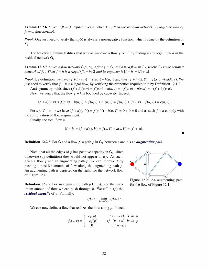
Lemma 12.2.6 Given a flow f defined over a network G, then the residual network G f together with c f

form a flow network.

Proof: One just need to verify that c f (·) is always a non-negative function, which is true by the definition ofE f .

The following lemma testifies that we can improve a flow f on G by finding a any legal flow h in theresidual netowrk G f .

Lemma 12.2.7 Given a flow network G(V, E), a flow f in G, and h be a flow in G f , where G f is the residualnetwork of f . . Then f + h is a (legal) flow in G and its capacity is | f + h| = | f | + |h|.

Proof: By definition, we have ( f + h)(u, v) = f (u, v)+ h(u, v) and thus ( f + h)(X,Y) = f (X,Y)+ h(X,Y). Wejust need to verify that f + h is a legal flow, by verifying the properties required to it by Definition 12.1.2.

Anti symmetry holds since ( f + h)(u, v) = f (u, v) + h(u, v) = − f (v, u) − h(v, u) = −( f + h)(v, u).Next, we verify that the flow f + h is bounded by capacity. Indeed,

( f + h)(u, v) ≤ f (u, v) + h(u, v) ≤ f (u, v) + c f (u, v) = f (u, v) + (c(u, v) − f (u, v)) = c(u, v).

For u ∈ V − s − t we have ( f + h)(u,V) = f (u,V) + h(u,V) = 0 + 0 = 0 and as such f + h comply withthe conservation of flow requirement.

Finally, the total flow is

| f + h| = ( f + h)(s,V) = f (s,V) + h(s,V) = | f | + |h| .

Definition 12.2.8 For G and a flow f , a path p in G f between s and t is an augmenting path.

Figure 12.2: An augmenting pathfor the flow of Figure 12.1.

Note, that all the edges of p has positive capacity in G f , sinceotherwise (by definition) they would not appear in E f . As such,given a flow f and an augmenting path p, we can improve f bypushing a positive amount of flow along the augmenting path p.An augmenting path is depicted on the right, for the network flowof Figure 12.1.

Definition 12.2.9 For an augmenting path p let c f (p) be the max-imum amount of flow we can push through p. We call c f (p) theresidual capacity of p. Formally,

c f (p) = min(u→v)∈p

c f (u, v).

We can now define a flow that realizes the flow along p. Indeed:

fp(u, v) =

c f (p) if (u→ v) is in p−c f (p) i f (v→ u) is in p

0 otherwise.

88

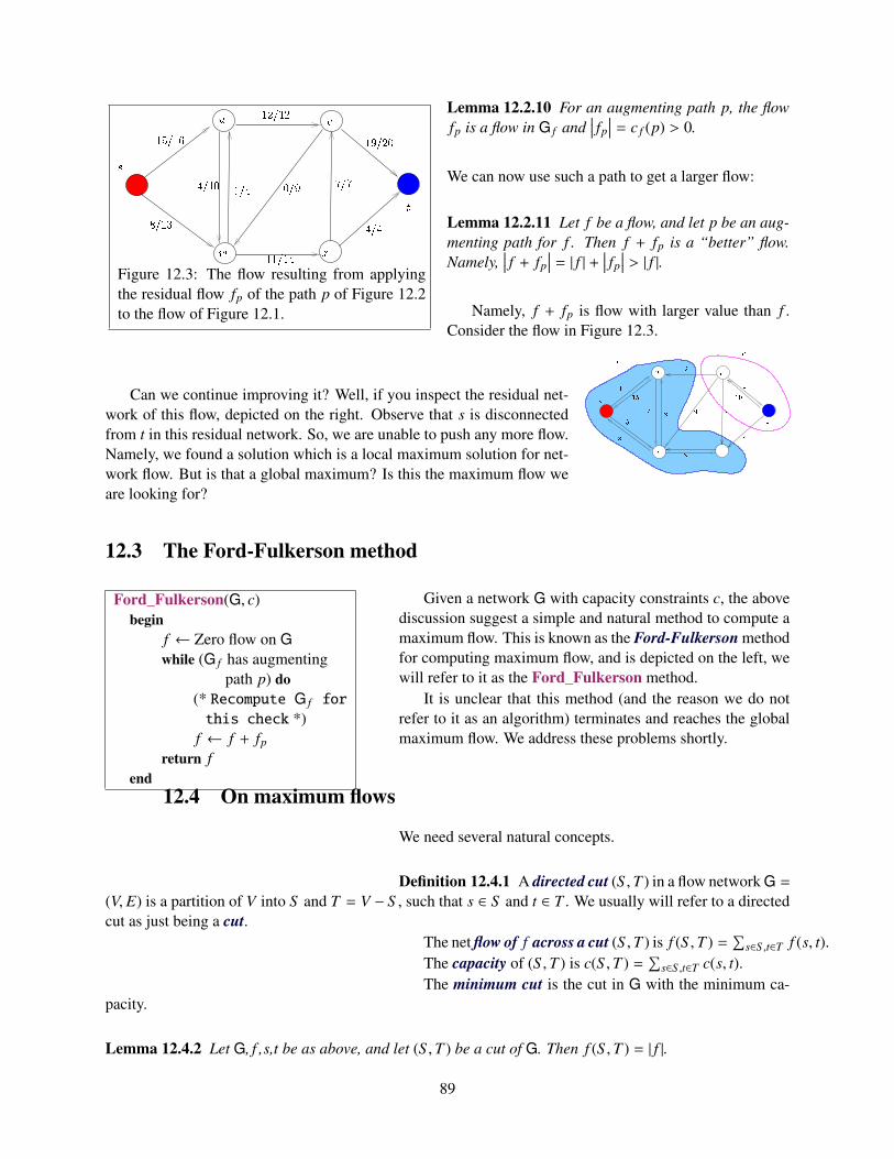
Figure 12.3: The flow resulting from applyingthe residual flow fp of the path p of Figure 12.2to the flow of Figure 12.1.

Lemma 12.2.10 For an augmenting path p, the flowfp is a flow in G f and

∣∣∣ fp∣∣∣ = c f (p) > 0.

We can now use such a path to get a larger flow:

Lemma 12.2.11 Let f be a flow, and let p be an aug-menting path for f . Then f + fp is a “better” flow.Namely,

∣∣∣ f + fp∣∣∣ = | f | + ∣∣∣ fp

∣∣∣ > | f |.Namely, f + fp is flow with larger value than f .

Consider the flow in Figure 12.3.

Can we continue improving it? Well, if you inspect the residual net-work of this flow, depicted on the right. Observe that s is disconnectedfrom t in this residual network. So, we are unable to push any more flow.Namely, we found a solution which is a local maximum solution for net-work flow. But is that a global maximum? Is this the maximum flow weare looking for?

12.3 The Ford-Fulkerson method

Ford_Fulkerson(G, c)begin

f ← Zero flow on Gwhile (G f has augmenting

path p) do(* Recompute G f forthis check *)

f ← f + fp

return fend

Given a network G with capacity constraints c, the abovediscussion suggest a simple and natural method to compute amaximum flow. This is known as the Ford-Fulkerson methodfor computing maximum flow, and is depicted on the left, wewill refer to it as the Ford_Fulkerson method.

It is unclear that this method (and the reason we do notrefer to it as an algorithm) terminates and reaches the globalmaximum flow. We address these problems shortly.

12.4 On maximum flows

We need several natural concepts.

Definition 12.4.1 A directed cut (S ,T ) in a flow network G =(V, E) is a partition of V into S and T = V − S , such that s ∈ S and t ∈ T . We usually will refer to a directedcut as just being a cut.

The net flow of f across a cut (S ,T ) is f (S ,T ) =∑

s∈S ,t∈T f (s, t).The capacity of (S ,T ) is c(S ,T ) =

∑s∈S ,t∈T c(s, t).

The minimum cut is the cut in G with the minimum ca-pacity.

Lemma 12.4.2 Let G, f ,s,t be as above, and let (S ,T ) be a cut of G. Then f (S ,T ) = | f |.

89

Proof: We have

f (S ,T ) = f (S ,V) − f (S , S ) = f (S ,V) = f (s,V) + f (S − s,V) = f (s,V) = | f | ,

since T = V \ S , and f (S − s,V) =∑

u∈S−s f (u,V) = 0 by Lemma 12.2.2 (v) (note that u can not be t ast ∈ T ).

Claim 12.4.3 The flow in a network is upper bounded by the capacity of any cut (S ,T ) in G.

Proof: Consider a cut (S ,T ). We have | f | = f (S ,T ) =∑

u∈S ,v∈T f (u, v) ≤∑

u∈S ,v∈T c(u, v) = c(S ,T ).

In particular, the maximum flow is bounded by the capacity of the minimum cut. Surprisingly, themaximum flow is exactly the value of the minimum cut.

Theorem 12.4.4 (Max-flow min-cut theorem.) If f is a flow in a flow network G = (V, E) with source sand sink t, then the following conditions are equivalent:

(A) f is a maximum flow in G

(B) The residual network G f contains no augmenting paths.

(C) | f | = c(S ,T ) for some cut (S ,T ) of G. And (S ,T ) is a minimum cut in G.

Proof: (A)⇒ (B): By contradiction. If there was an augmenting path p then c f (p) > 0, and we can generatea new flow f + fp, such that

∣∣∣ f + fp∣∣∣ = | f | + c f (p) > | f | . A contradiction as f is a maximum flow.

(B)⇒ (C): Well, it must be that s and t are disconnected in G f . Let

S =v

∣∣∣∣ Exists a path between s and v in G f

and T = V \ S . We have that s ∈ S , t ∈ T , and for any u ∈ S and v ∈ T we have f (u, v) = c(u, v). Indeed, ifthere were u ∈ S and v ∈ T such that f (u, v) < c(u, v) then (u→ v) ∈ E f , and v would be reachable from sin G f , contradicting the construction of T .

This implies that | f | = f (S ,T ) = c(S ,T ). The cut (S ,T ) must be a minimum cut, because otherwisethere would be cut (S ′,T ′) with smaller capacity c(S ′,T ′) < c(S ,T ) = f (S ,T ) = | f |, On the other hand, byLemma 12.4.3, we have | f | = f (S ′,T ′) ≤ c(S ′,T ′). A contradiction.

(C)⇒ (A) Well, for any cut (U,V), we know that | f | ≤ c(U,V). This implies that if | f | = c(S ,T ) thenthe flow can not be any larger, and it is thus a maximum flow.

The above max-flow min-cut theorem implies that if Ford_Fulkerson terminates, then it had computedthe maximum flow. What is still allusive is showing that the Ford_Fulkerson method always terminates.This turns out to be correct only if we are careful about the way we pick the augmenting path.

90

Chapter 13

Network Flow II - The Vengeance

13.1 Accountability

Figure 13.1: http://www.cs.berkeley.edu/~jrs/

The comic in Figure 13.1 is by Jonathan Shewchukand is referring to the Calvin and Hobbes comics.

People that do not know maximum flows: es-sentially everybody.

Average salary on earth < $5, 000People that know maximum flow - most of

them work in programming related jobs and makeat least $10, 000 a year.

Salary of people that learned maximum flows:> $10, 000

Salary of people that did not learn maximumflows: < $5, 000

Salary of people that know Latin: 0 (unem-ployed).

Thus, by just learning maximum flows (and not knowing Latin) you can double your future salary!

13.2 Ford-Fulkerson Method

Ford-Fulkerson(G,s,t)Initialize flow f to zerowhile ∃ path π from s to t in G f do

c f (π)← minc f (u, v)

∣∣∣∣ (u→ v) ∈ π

for ∀ (u→ v) ∈ π dof (u, v)← f (u, v) + c f (π)f (v, u)← f (v, u) − c f (π)

The Ford-Fulkerson method is depicted on the right.

Lemma 13.2.1 If the capacities on the edges of G are inte-gers, then Ford-Fulkerson runs in O(m | f ∗|) time, where | f ∗|is the amount of flow in the maximum flow and m = |E(G)|.

Proof: Observe that the Ford-Fulkerson method per-forms only subtraction,addition and min operations. Thus,if it finds an augmenting path π, then c f (π) must be a positiveinteger number. Namely, c f (π) ≥ 1. Thus, | f ∗| must be aninteger number (by induction), and each iteration of the algorithm improves the flow by at least 1. It followsthat after | f ∗| iterations the algorithm stops. Each iteration takes O(m + n) = O(m) time, as can be easilyverified.

The following observation is an easy consequence of our discussion.

91

http://www.cs.berkeley.edu/~jrs/

http://www.cs.berkeley.edu/~jrs/

Observation 13.2.2 (Integrality theorem.) If the capacity function c takes on only integral values, thenthe maximum flow f produced by the Ford-Fulkerson method has the property that | f | is integer-valued.Moreover, for all vertices u and v, the value of f (u, v) is also an integer.

13.3 The Edmonds-Karp algorithm

The Edmonds-Karp algorithm works by modifying the Ford-Fulkerson method so that it always returnsthe shortest augmenting path in G f (i.e., path with smallest number of edges). This is implemented byfinding π using BFS in G f .

Definition 13.3.1 For a flow f , let δ f (v) be the length of the shortest path from the source s to v in theresidual graph G f . Each edge is considered to be of length 1.

We will shortly prove that for any vertex v ∈ V \ s, t the function δ f (v), in the residual networkG f , increases monotonically with each flow augmentation. We delay proving this (key) technical fact (seeLemma 13.3.5 below), and first show its implications.

Lemma 13.3.2 During the execution of the Edmonds-Karp algorithm, an edge (u→ v) might disappear(and thus reappear) from G f at most n/2 times throughout the execution of the algorithm, where n = |V(G)|.

Proof: Consider an iteration when the edge (u→ v) disappears. Clearly, in this iteration the edge (u→ v)appeared in the augmenting path π. In fact, this edge was fully utilized; namely, c f (π) = c f (uv), where fis the flow in the beginning of the iteration when it disappeared. We continue running Edmonds-Karp till(u→ v) “magically” reappears. This means that in the iteration before (u→ v) reappeared in the residualgraph, the algorithm handled an augmenting path σ that contained the edge (v→ u). Let g be the flow usedto compute σ. We have, by the monotonicity of δ(·) [i.e., Lemma 13.3.5 below], that

δg(u) = δg(v) + 1 ≥ δ f (v) + 1 = δ f (u) + 2

as Edmonds-Karp is always augmenting along the shortest path. Namely, the distance of s to u had in-creased by 2 between its disappearance and its (magical?) reappearance. Since δ0(u) ≥ 0 and the maximumvalue of δ?(u) is n, it follows that (u→ v) can disappear and reappear at most n/2 times during the executionof the Edmonds-Karp algorithm.

(The careful reader would observe that in fact δ?(u) might become infinity at some point during thealgorithm execution (i.e., u is no longer reachable from s). If so, by monotonicity, the edge (u→ v) wouldnever appear again, in the residual graph, in any future iteration of the algorithm.

Observation 13.3.3 Every time we add an augmenting path during the execution of the Edmonds-Karpalgorithm, at least one edge disappears from the residual graph G?. Indeed, every edge that realizes theresidual capacity of the augmenting path will disappear once we push the maximum possible flow along thispath.

Lemma 13.3.4 The Edmonds-Karp algorithm handles at most O(nm) augmenting paths before it stops.Its running time is O

(nm2

), where n = |V(G)| and m = |E(G)|.

Proof: Every edge might disappear at most n/2 times during Edmonds-Karp execution, by Lemma 13.3.2.Thus, there are at most nm/2 edge disappearances during the execution of the Edmonds-Karp algorithm.At each iteration, we perform path augmentation, and at least one edge disappears along it from the residualgraph. Thus, the Edmonds-Karp algorithm perform at most O(mn) iterations.

92

Performing a single iteration of the algorithm boils down to computing an Augmenting path. Computingsuch a path takes O(m) time as we have to perform BFS to find the augmenting path. It follows, that theoverall running time of the algorithm is O

(nm2

).

We still need to prove the aforementioned monotonicity property. (This is the only part in our discussionof network flow where the argument gets a bit tedious. So bear with us, after all, you are going to doubleyour salary here.)

Lemma 13.3.5 If the Edmonds-Karp algorithm is run on a flow network G = (V, E) with source s and sinkt, then for all vertices v ∈ V \ s, t, the shortest path distance δ f (v) in the residual network G f increasesmonotonically with each flow augmentation.

Proof: Assume, for the sake of contradiction, that this is false. Consider the flow just after the firstiteration when this claim failed. Let f denote the flow before this (fatal) iteration was performed, and let gbe the flow after.

Let v be the vertex such that δg(v) is minimal, among all vertices for which the monotonicity fails.Formally, this is the vertex v where δg(v) is minimal and δg(v) < δ f (v).

Let π = s → · · · → u → v be the shortest path in Gg from s to v. Clearly, (u→ v) ∈ E(Gg

), and thus

δg(u) = δg(v) − 1.By the choice of v it must be that δg(u) ≥ δ f (u), since otherwise the monotonicity property fails for u,

and u is closer to s than v in Gg. This contradicts our choice of v as being the closest vertex to s that failsthe monotonicity property. There are now two possibilities:

(i) If (u→ v) ∈ E(G f

)then

δ f (v) ≤ δ f (u) + 1 ≤ δg(u) + 1 = δg(v) − 1 + 1 = δg(v).

This contradicts our assumptions that δ f (v) > δg(v).(ii) If (u→ v) is not in E

(G f

)then the augmenting path π used in computing g from f contains the edge

(v→ u). Indeed, the edge (u→ v) reappeared in the residual graph Gg (while not being present in G f ).The only way this can happens is if the augmenting path π pushed a flow in the other direction on the edge(u→ v). Namely, (v→ u) ∈ π. However, the algorithm always augment along the shortest path. Thus, sinceby assumption δg(v) < δ f (v), we have

δ f (u) = δ f (v) + 1 > δg(v) = δg(u) + 1,

by the definition of u.Thus, δ f (u) > δg(u) (i.e., the monotonicity property fails for u) and δg(u) < δg(v). A contradiction to the

choice of v.

13.4 Applications and extensions for Network Flow

13.4.1 Maximum Bipartite Matching

Definition 13.4.1 For an undirected graph G = (V, E) a matching is a subset of edges M ⊆ E such that forall vertices v ∈ V , at most one edge of M is incident on v. A maximum matching is a matching M such thatfor any matching M′ we have |M| ≥ |M′|.

A matching is perfect if it involves all vertices. See Figure 13.2 for examples of these definitions.

Theorem 13.4.2 One can compute maximum bipartite matching using network flow in O(nm2) time, for abipartite graph with n vertices and m edges.

93

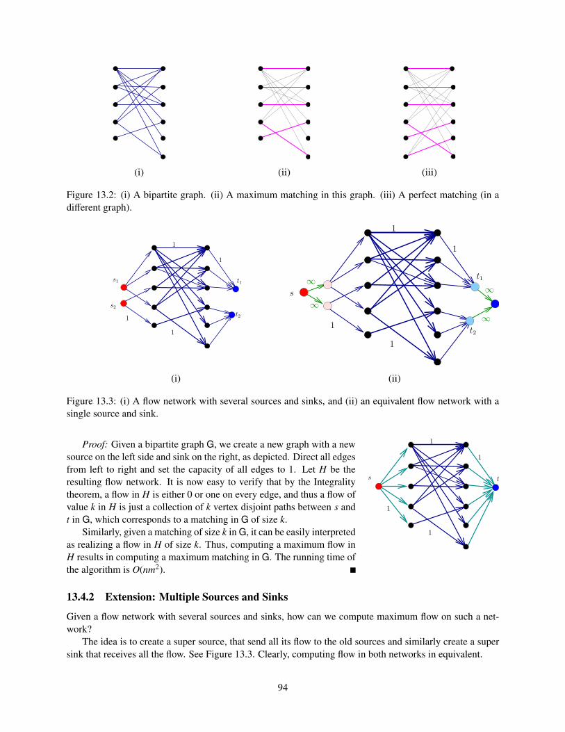
(i) (ii) (iii)

Figure 13.2: (i) A bipartite graph. (ii) A maximum matching in this graph. (iii) A perfect matching (in adifferent graph).

1

1

1

1

s1

s2

t1

t2

1

1

1

1

t1

s

t2

∞

∞

∞

∞

(i) (ii)

Figure 13.3: (i) A flow network with several sources and sinks, and (ii) an equivalent flow network with asingle source and sink.

ts

1

1

1

1

Proof: Given a bipartite graph G, we create a new graph with a newsource on the left side and sink on the right, as depicted. Direct all edgesfrom left to right and set the capacity of all edges to 1. Let H be theresulting flow network. It is now easy to verify that by the Integralitytheorem, a flow in H is either 0 or one on every edge, and thus a flow ofvalue k in H is just a collection of k vertex disjoint paths between s andt in G, which corresponds to a matching in G of size k.

Similarly, given a matching of size k in G, it can be easily interpretedas realizing a flow in H of size k. Thus, computing a maximum flow inH results in computing a maximum matching in G. The running time ofthe algorithm is O(nm2).

13.4.2 Extension: Multiple Sources and Sinks

Given a flow network with several sources and sinks, how can we compute maximum flow on such a net-work?

The idea is to create a super source, that send all its flow to the old sources and similarly create a supersink that receives all the flow. See Figure 13.3. Clearly, computing flow in both networks in equivalent.

94

Chapter 14

Network Flow III - Applications

14.1 Edge disjoint paths

14.1.1 Edge-disjoint paths in a directed graphs

Question 14.1.1 Given a graph G (either directed or undirected), two vertices s and t, and a parameter k,the task is to compute k paths from s to t in G, such that they are edge disjoint; namely, these paths do notshare an edge.

To solve this problem, we will convert G (assume G is a directed graph for the time being) into a networkflow graph H, such that every edge has capacity 1. Find the maximum flow in G (between s and t). Weclaim that the value of the maximum flow in the network H, is equal to the number of edge disjoint paths inG.

Lemma 14.1.2 If there are k edge disjoint paths in G between s and t, then the maximum flow in H is atleast k.

Proof: Given k such edge disjoint paths, push one unit of flow along each such path. The resulting flow islegal in h and it has value k.

Definition 14.1.3 (0/1-flow.) A flow f is 0/1-flow if every edge has either no flow on it, or one unit of flow.

Lemma 14.1.4 Let f be a 0/1 flow in a network H with flow value µ. Then there are µ edge disjoint pathsbetween s and t in H.

Proof: By induction on the number of edges in H that has one unit of flow assigned to them by f . Ifµ = 0 then there is nothing to prove.

Otherwise, start traversing the graph H from s traveling only along edges with flow 1 assigned to themby f . We mark such an edge as used, and do not allow one to travel on such an edge again. There are twopossibilities:

(i) We reached the target vertex t. In this case, we take this path, add it to the set of output paths, andreduce the flow along the edges of the generated path π to 0. Let H′ be the resulting flow network and f ′ theresulting flow. We have | f ′| = µ − 1, H′ has less edges, and by induction, it has µ − 1 edge disjoint paths inH′ between s and t. Together with π this forms µ such paths.

(ii) We visit a vertex v for the second time. In this case, our traversal contains a cycle C, of edges inH that have flow 1 on them. We set the flow along the edges of C to 0 and use induction on the remaining

95

graph (since it has less edges with flow 1 on them). The value of the flow f did not change by removing C,and as such it follows by induction that there are µ edge disjoint paths between s and t in H.

Since the graph G is simple, there are at most n = |V(H)| edges that leave s. As such, the maximum flowin H is n. Thus, applying the Ford-Fulkerson algorithm, takes O(mn) time. The extraction of the paths canalso be done in linear time by applying the algorithm in the proof of Lemma 14.1.4. As such, we get:

Theorem 14.1.5 Given a directed graph G with n vertices and m edges, and two vertices s and t, one cancompute the maximum number of edge disjoint paths between s and t in H, in O(mn) time.

As a consequence we get the following cute result:

Lemma 14.1.6 In a directed graph G with nodes s and t the maximum number of edge disjoint s − t pathsis equal to the minimum number of edges whose removal separates s from t.

Proof: Let U be a collection of edge-disjoint paths from s to t in G. If we remove a set F of edges fromG and separate s from t, then it must be that every path in U uses at least one edge of F. Thus, the numberof edge-disjoint paths is bounded by the number of edges needed to be removed to separate s and t. Namely,|U | ≤ |F|.

As for the other direction, let F be a set of edges thats its removal separates s and t. We claim that theset F form a cut in G between s and t. Indeed, let S be the set of all vertices in G that are reachable froms without using an edge of F. Clearly, if F is minimal then it must be all the edges of the cut (S ,T ) (inparticular, if F contains some edge which is not in (S ,T ) we can remove it and get a smaller separating setof edges). In particular, the smallest set F with this separating property has the same size as the minimumcut between s and t in G, which is by the max-flow mincut theorem, also the maximum flow in the graph G(where every edge has capacity 1).

But then, by Theorem 14.1.5, there are |F| edge disjoint paths in G (since |F| is the amount of themaximum flow).

14.1.2 Edge-disjoint paths in undirected graphs

We would like to solve the s-t disjoint path problem for an undirected graph.

Problem 14.1.7 Given undirected graph G, s and t, find the maximum number of edge-disjoint paths in Gbetween s and t.

The natural approach is to duplicate every edge in the undirected graph G, and get a (new) directed graphH. Next, apply the algorithm of Section 14.1.1 to H.

So compute for H the maximum flow f (where every edge has capacity 1). The problem is the flow fmight use simultaneously the two edges (u→ v) and (v→ u). Observe, however, that in such case we canremove both edges from the flow f . In the resulting flow is legal and has the same value. As such, if werepeatedly remove those “double edges” from the flow f , the resulting flow f ′ has the same value. Next, weextract the edge disjoint paths from the graph, and the resulting paths are now edge disjoint in the originalgraph.

Lemma 14.1.8 There are k edge-disjoint paths in an undirected graph G from s to t if and only if themaximum value of an s− t flow in the directed version H of G is at least k. Furthermore, the Ford-Fulkersonalgorithm can be used to find the maximum set of disjoint s-t paths in G in O(mn) time.

96

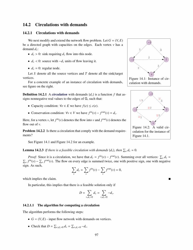
14.2 Circulations with demands

14.2.1 Circulations with demands

−3

−3

2

4

3 3

22

2

Figure 14.1: Instance of cir-culation with demands.

We next modify and extend the network flow problem. Let G = (V, E)be a directed graph with capacities on the edges. Each vertex v has ademand dv:• dv > 0: sink requiring dv flow into this node.

• dv < 0: source with −dv units of flow leaving it.

• dv = 0: regular node.

Let S denote all the source vertices and T denote all the sink/targetvertices.

For a concrete example of an instance of circulation with demands,see figure on the right.

−3

−3

2

4

3 3

22

2

1/2/

2/2/

2/

Figure 14.2: A valid cir-culation for the instance ofFigure 14.1.

Definition 14.2.1 A circulation with demands dv is a function f that as-signs nonnegative real values to the edges of G, such that:

• Capacity condition: ∀e ∈ E we have f (e) ≤ c(e).

• Conservation condition: ∀v ∈ V we have f in(v) − f out(v) = dv.

Here, for a vertex v, let f in(v) denotes the flow into v and f out(v) denotes theflow out of v.

Problem 14.2.2 Is there a circulation that comply with the demand require-ments?

See Figure 14.1 and Figure 14.2 for an example.

Lemma 14.2.3 If there is a feasible circulation with demands dv, then∑

v dv = 0.

Proof: Since it is a circulation, we have that dv = f in(v) − f out(v). Summing over all vertices:∑

v dv =∑v f in(v) −

∑v f out(v). The flow on every edge is summed twice, one with positive sign, one with negative

sign. As such, ∑v

dv =∑

v

f in(v) −∑

v

f out(v) = 0,

which implies the claim.

In particular, this implies that there is a feasible solution only if

D =∑

v,dv>0

dv =∑

v,dv<0

−dv.

14.2.1.1 The algorithm for computing a circulation

The algorithm performs the following steps:

• G = (V, E) - input flow network with demands on vertices.

• Check that D =∑

v,dv>0 dv =∑

v,dv<0 −dv.

97

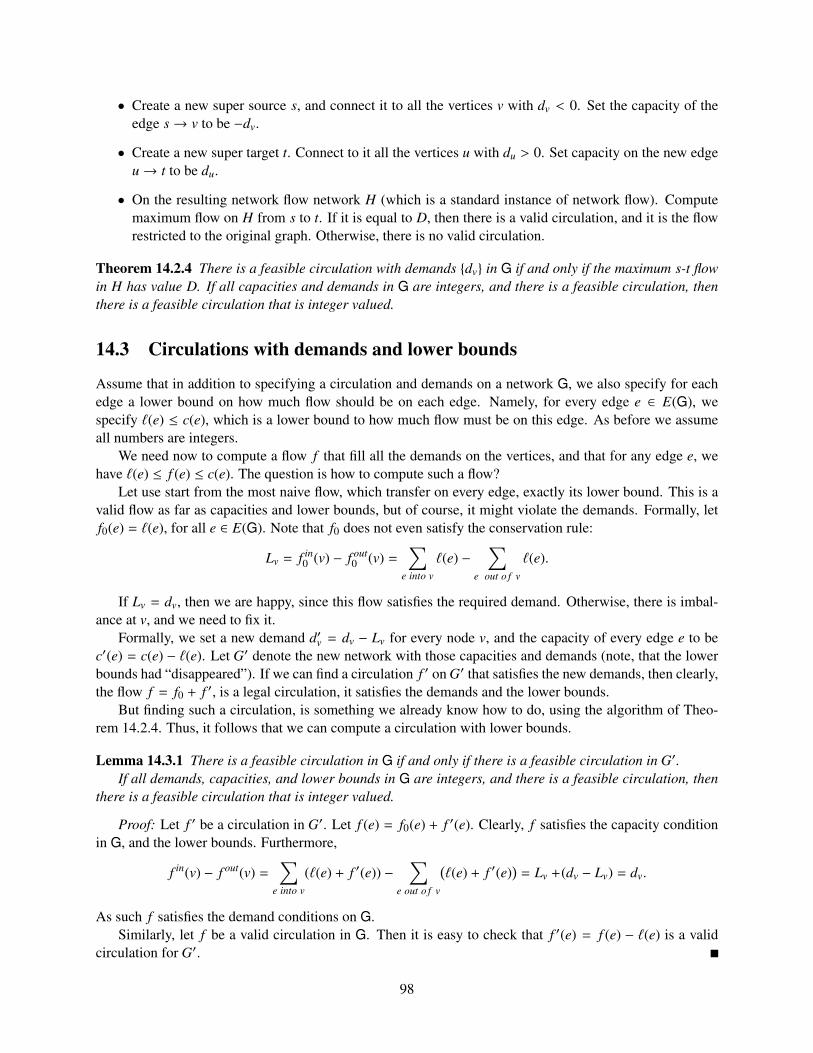
• Create a new super source s, and connect it to all the vertices v with dv < 0. Set the capacity of theedge s→ v to be −dv.

• Create a new super target t. Connect to it all the vertices u with du > 0. Set capacity on the new edgeu→ t to be du.

• On the resulting network flow network H (which is a standard instance of network flow). Computemaximum flow on H from s to t. If it is equal to D, then there is a valid circulation, and it is the flowrestricted to the original graph. Otherwise, there is no valid circulation.

Theorem 14.2.4 There is a feasible circulation with demands dv in G if and only if the maximum s-t flowin H has value D. If all capacities and demands in G are integers, and there is a feasible circulation, thenthere is a feasible circulation that is integer valued.

14.3 Circulations with demands and lower bounds

Assume that in addition to specifying a circulation and demands on a network G, we also specify for eachedge a lower bound on how much flow should be on each edge. Namely, for every edge e ∈ E(G), wespecify `(e) ≤ c(e), which is a lower bound to how much flow must be on this edge. As before we assumeall numbers are integers.

We need now to compute a flow f that fill all the demands on the vertices, and that for any edge e, wehave `(e) ≤ f (e) ≤ c(e). The question is how to compute such a flow?

Let use start from the most naive flow, which transfer on every edge, exactly its lower bound. This is avalid flow as far as capacities and lower bounds, but of course, it might violate the demands. Formally, letf0(e) = `(e), for all e ∈ E(G). Note that f0 does not even satisfy the conservation rule:

Lv = f in0 (v) − f out

0 (v) =∑

e into v

`(e) −∑

e out o f v

`(e).

If Lv = dv, then we are happy, since this flow satisfies the required demand. Otherwise, there is imbal-ance at v, and we need to fix it.

Formally, we set a new demand d′v = dv − Lv for every node v, and the capacity of every edge e to bec′(e) = c(e) − `(e). Let G′ denote the new network with those capacities and demands (note, that the lowerbounds had “disappeared”). If we can find a circulation f ′ on G′ that satisfies the new demands, then clearly,the flow f = f0 + f ′, is a legal circulation, it satisfies the demands and the lower bounds.

But finding such a circulation, is something we already know how to do, using the algorithm of Theo-rem 14.2.4. Thus, it follows that we can compute a circulation with lower bounds.

Lemma 14.3.1 There is a feasible circulation in G if and only if there is a feasible circulation in G′.If all demands, capacities, and lower bounds in G are integers, and there is a feasible circulation, then

there is a feasible circulation that is integer valued.

Proof: Let f ′ be a circulation in G′. Let f (e) = f0(e) + f ′(e). Clearly, f satisfies the capacity conditionin G, and the lower bounds. Furthermore,

f in(v) − f out(v) =∑

e into v

(`(e) + f ′(e)) −∑

e out o f v

(`(e) + f ′(e)

)= Lv +(dv − Lv) = dv.

As such f satisfies the demand conditions on G.Similarly, let f be a valid circulation in G. Then it is easy to check that f ′(e) = f (e) − `(e) is a valid

circulation for G′.

98

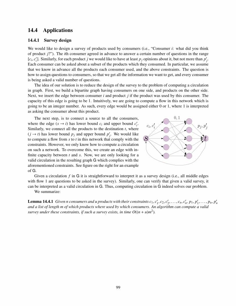
14.4 Applications

14.4.1 Survey design

We would like to design a survey of products used by consumers (i.e., “Consumer i: what did you thinkof product j?”). The ith consumer agreed in advance to answer a certain number of questions in the range[ci, c′i]. Similarly, for each product j we would like to have at least p j opinions about it, but not more than p′j.Each consumer can be asked about a subset of the products which they consumed. In particular, we assumethat we know in advance all the products each consumer used, and the above constraints. The question ishow to assign questions to consumers, so that we get all the information we want to get, and every consumeris being asked a valid number of questions.

The idea of our solution is to reduce the design of the survey to the problem of computing a circulationin graph. First, we build a bipartite graph having consumers on one side, and products on the other side.Next, we insert the edge between consumer i and product j if the product was used by this consumer. Thecapacity of this edge is going to be 1. Intuitively, we are going to compute a flow in this network which isgoing to be an integer number. As such, every edge would be assigned either 0 or 1, where 1 is interpretedas asking the consumer about this product.

s

0, 1

ci, c′

i

t

pj, p′

j

The next step, is to connect a source to all the consumers,where the edge (s→ i) has lower bound ci and upper bound c′i .Similarly, we connect all the products to the destination t, where( j→ t) has lower bound p j and upper bound p′j. We would liketo compute a flow from s to t in this network that comply with theconstraints. However, we only know how to compute a circulationon such a network. To overcome this, we create an edge with in-finite capacity between t and s. Now, we are only looking for avalid circulation in the resulting graph G which complies with theaforementioned constraints. See figure on the right for an exampleof G.

Given a circulation f in G it is straightforward to interpret it as a survey design (i.e., all middle edgeswith flow 1 are questions to be asked in the survey). Similarly, one can verify that given a valid survey, itcan be interpreted as a valid circulation in G. Thus, computing circulation in G indeed solves our problem.

We summarize:

Lemma 14.4.1 Given n consumers and u products with their constraints c1, c′1, c2, c′2, . . . , cn, c′n, p1, p′1, . . . , pu, p′uand a list of length m of which products where used by which consumers. An algorithm can compute a validsurvey under these constraints, if such a survey exists, in time O((n + u)m2).

99

100

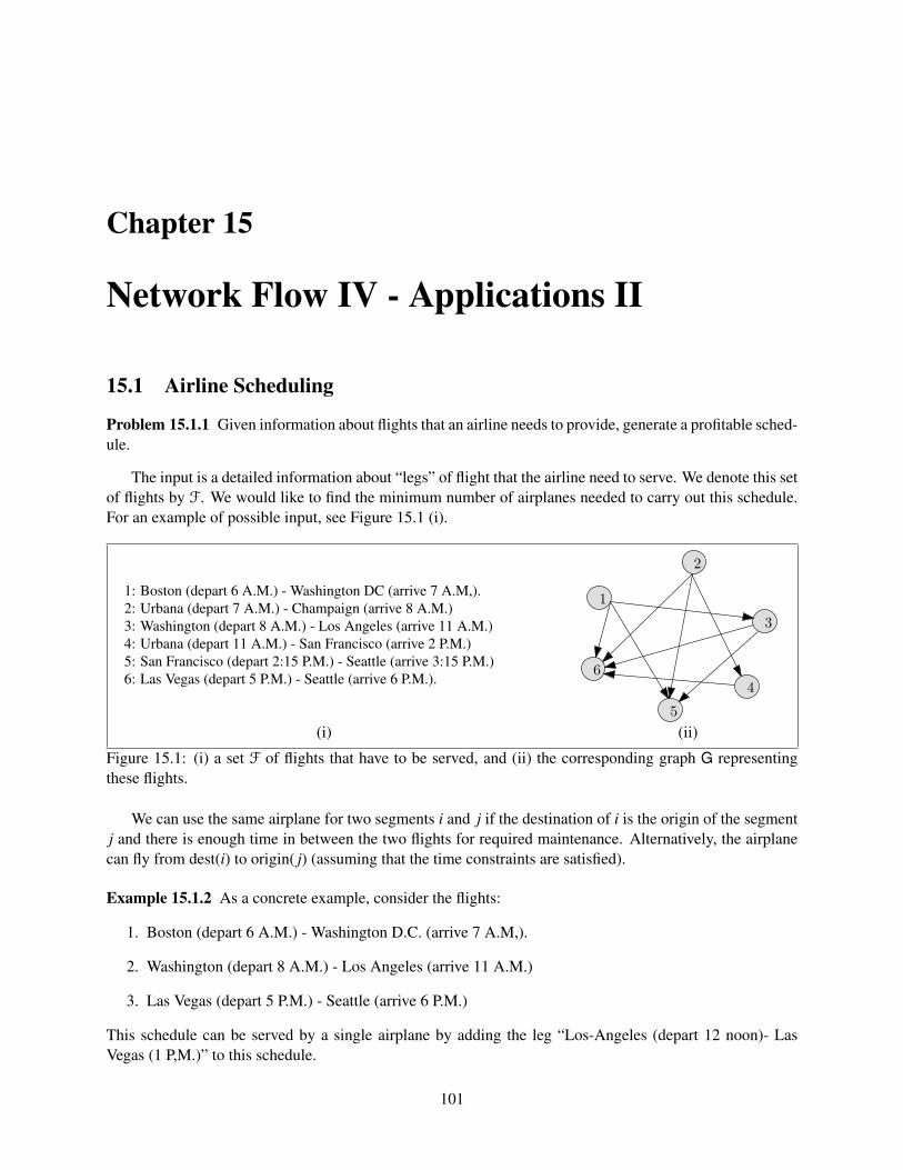
Chapter 15

Network Flow IV - Applications II

15.1 Airline Scheduling

Problem 15.1.1 Given information about flights that an airline needs to provide, generate a profitable sched-ule.

The input is a detailed information about “legs” of flight that the airline need to serve. We denote this setof flights by F. We would like to find the minimum number of airplanes needed to carry out this schedule.For an example of possible input, see Figure 15.1 (i).

1: Boston (depart 6 A.M.) - Washington DC (arrive 7 A.M,).2: Urbana (depart 7 A.M.) - Champaign (arrive 8 A.M.)3: Washington (depart 8 A.M.) - Los Angeles (arrive 11 A.M.)4: Urbana (depart 11 A.M.) - San Francisco (arrive 2 P.M.)5: San Francisco (depart 2:15 P.M.) - Seattle (arrive 3:15 P.M.)6: Las Vegas (depart 5 P.M.) - Seattle (arrive 6 P.M.).

1

2

3

4

5

6

(i) (ii)

Figure 15.1: (i) a set F of flights that have to be served, and (ii) the corresponding graph G representingthese flights.

We can use the same airplane for two segments i and j if the destination of i is the origin of the segmentj and there is enough time in between the two flights for required maintenance. Alternatively, the airplanecan fly from dest(i) to origin( j) (assuming that the time constraints are satisfied).

Example 15.1.2 As a concrete example, consider the flights:

1. Boston (depart 6 A.M.) - Washington D.C. (arrive 7 A.M,).

2. Washington (depart 8 A.M.) - Los Angeles (arrive 11 A.M.)

3. Las Vegas (depart 5 P.M.) - Seattle (arrive 6 P.M.)

This schedule can be served by a single airplane by adding the leg “Los-Angeles (depart 12 noon)- LasVegas (1 P,M.)” to this schedule.

101

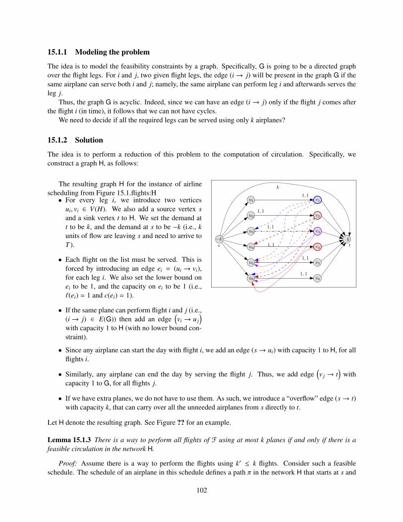
15.1.1 Modeling the problem

The idea is to model the feasibility constraints by a graph. Specifically, G is going to be a directed graphover the flight legs. For i and j, two given flight legs, the edge (i→ j) will be present in the graph G if thesame airplane can serve both i and j; namely, the same airplane can perform leg i and afterwards serves theleg j.

Thus, the graph G is acyclic. Indeed, since we can have an edge (i→ j) only if the flight j comes afterthe flight i (in time), it follows that we can not have cycles.

We need to decide if all the required legs can be served using only k airplanes?

15.1.2 Solution

The idea is to perform a reduction of this problem to the computation of circulation. Specifically, weconstruct a graph H, as follows:

u1 v1

u2 v2

u3 v3

u4 v4

u5 v5

u6 v6

1, 1

1, 1

1, 1

1, 1

1, 1

1, 1

−k

skt

kThe resulting graph H for the instance of airline

scheduling from Figure 15.1.flights:H• For every leg i, we introduce two vertices

ui, vi ∈ V(H). We also add a source vertex sand a sink vertex t to H. We set the demand att to be k, and the demand at s to be −k (i.e., kunits of flow are leaving s and need to arrive toT ).

• Each flight on the list must be served. This isforced by introducing an edge ei = (ui → vi),for each leg i. We also set the lower bound onei to be 1, and the capacity on ei to be 1 (i.e.,`(ei) = 1 and c(ei) = 1).

• If the same plane can perform flight i and j (i.e.,(i→ j) ∈ E(G)) then add an edge

(vi → u j

)with capacity 1 to H (with no lower bound con-straint).

• Since any airplane can start the day with flight i, we add an edge (s→ ui) with capacity 1 to H, for allflights i.

• Similarly, any airplane can end the day by serving the flight j. Thus, we add edge(v j → t

)with

capacity 1 to G, for all flights j.

• If we have extra planes, we do not have to use them. As such, we introduce a “overflow” edge (s→ t)with capacity k, that can carry over all the unneeded airplanes from s directly to t.

Let H denote the resulting graph. See Figure ?? for an example.

Lemma 15.1.3 There is a way to perform all flights of F using at most k planes if and only if there is afeasible circulation in the network H.

Proof: Assume there is a way to perform the flights using k′ ≤ k flights. Consider such a feasibleschedule. The schedule of an airplane in this schedule defines a path π in the network H that starts at s and

102

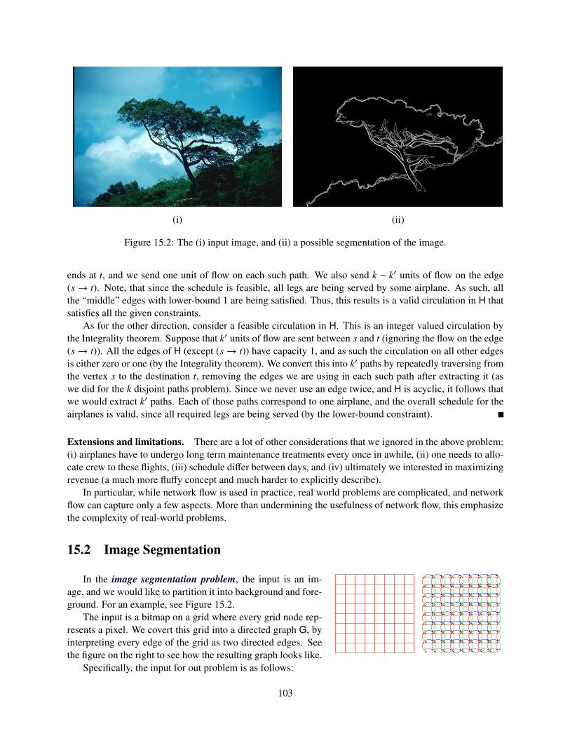
(i) (ii)

Figure 15.2: The (i) input image, and (ii) a possible segmentation of the image.

ends at t, and we send one unit of flow on each such path. We also send k − k′ units of flow on the edge(s→ t). Note, that since the schedule is feasible, all legs are being served by some airplane. As such, allthe “middle” edges with lower-bound 1 are being satisfied. Thus, this results is a valid circulation in H thatsatisfies all the given constraints.

As for the other direction, consider a feasible circulation in H. This is an integer valued circulation bythe Integrality theorem. Suppose that k′ units of flow are sent between s and t (ignoring the flow on the edge(s→ t)). All the edges of H (except (s→ t)) have capacity 1, and as such the circulation on all other edgesis either zero or one (by the Integrality theorem). We convert this into k′ paths by repeatedly traversing fromthe vertex s to the destination t, removing the edges we are using in each such path after extracting it (aswe did for the k disjoint paths problem). Since we never use an edge twice, and H is acyclic, it follows thatwe would extract k′ paths. Each of those paths correspond to one airplane, and the overall schedule for theairplanes is valid, since all required legs are being served (by the lower-bound constraint).

Extensions and limitations. There are a lot of other considerations that we ignored in the above problem:(i) airplanes have to undergo long term maintenance treatments every once in awhile, (ii) one needs to allo-cate crew to these flights, (iii) schedule differ between days, and (iv) ultimately we interested in maximizingrevenue (a much more fluffy concept and much harder to explicitly describe).

In particular, while network flow is used in practice, real world problems are complicated, and networkflow can capture only a few aspects. More than undermining the usefulness of network flow, this emphasizethe complexity of real-world problems.

15.2 Image Segmentation

In the image segmentation problem, the input is an im-age, and we would like to partition it into background and fore-ground. For an example, see Figure 15.2.

The input is a bitmap on a grid where every grid node rep-resents a pixel. We covert this grid into a directed graph G, byinterpreting every edge of the grid as two directed edges. Seethe figure on the right to see how the resulting graph looks like.

Specifically, the input for out problem is as follows:

103

• A bitmap of size N × N, with an associated directed graph G = (V, E).

• For every pixel i, we have a value fi ≥ 0, which is an estimate of the likelihood of this pixel to be inforeground (i.e., the larger fi is the more probable that it is in the foreground)

• For every pixel i, we have (similarly) an estimate bi of the likelihood of pixel i to be in background.

• For every two adjacent pixels i and j we have a separation penalty pi j, which is the “price” of separat-ing i from j. This quantity is defined only for adjacent pixels in the bitmap. (For the sake of simplicityof exposition we assume that pi j = p ji. Note, however, that this assumption is not necessary for ourdiscussion.)

Problem 15.2.1 Given input as above, partition V (the set of pixels) into two disjoint subsets F and B, suchthat

q(F, B) =∑i∈F

fi +∑i∈B

bi −∑

(i, j)∈E,|F∩i, j|=1

pi j.

is maximized.

We can rewrite q(F, B) as:

q(F, B) =∑i∈F

fi +∑j∈B

b j −∑

(i, j)∈E,|F∩i, j|=1

pi j =∑i∈v

( fi + bi) −∑i∈B

fi −∑j∈F

b j −∑

(i, j)∈E,|F∩i, j|=1

pi j.

Since the term∑

i∈v( fi + bi) is a constant, maximizing q(F, B) is equivalent to minimizing u(F, B), where

u(F, B) =∑i∈B

fi +∑j∈F

b j +∑

(i, j)∈E,|F∩i, j|=1

pi j. (15.1)

How do we compute this partition. Well, the basic idea is to compute a minimum cut in a graph such thatsits price would correspond to u(F, B). Before dwelling into the exact details, it is useful to play around withsome toy examples to get some intuition. Note, that we are using the max-flow algorithm as an algorithmfor computing minimum directed cut.

s i tfi biTo begin with, consider a graph having a source s, a vertex i, and a sink t. We

set the price of (s→ i) to be fi and the price of the edge (i→ t) to be bi. Clearly,there are two possible cuts in the graph, either (s, i , t) (with a price bi) or (s , i, t) (with a price fi). Inparticular, every path of length 2 in the graph between s and t forces the algorithm computing the minimum-cut (via network flow) to choose one of the edges, to the cut, where the algorithm “prefers” the edge withlower price.

si

tfi

bi

j bjfj

Next, consider a bitmap with two vertices i an j that are adjacent. Clearly, min-imizing the first two terms in Eq. (15.1) is easy, by generating length two parallelpaths between s and t through i and j. See figure on the right. Clearly, the price of acut in this graph is exactly the price of the partition of i, j into background and foreground sets. However,this ignores the separation penalty pi j.

sifi

bi

j bjfj

tpij pij

To this end, we introduce two new edges (i→ j) and ( j→ i) into the graphand set their price to be pi j. Clearly, a price of a cut in the graph can beinterpreted as the value of u(F, B) of the corresponding sets F and B, since allthe edges in the segmentation from nodes of F to nodes of B are contributing their separation price to the cutprice. Thus, if we extend this idea to the directed graph G, the minimum-cut in the resulting graph wouldcorresponds to the required segmentation.

104

Let us recap: Given the directed grid graph G = (V, E) we add two special source and sink vertices,denoted by s and t respectively. Next, for all the pixels i ∈ V , we add an edge ei = (s→ i) to the graph,setting its capacity to be c(ei) = fi. Similarly, we add the edge e′i = ( j→ t) with capacity c(e′i) = bi.Similarly, for every pair of vertices i. j in that grid that are adjacent, we assign the cost pi j to the edges(i→ j) and ( j→ i). Let H denote the resulting graph.

The following lemma, follows by the above discussion.

Lemma 15.2.2 A minimum cut (F, B) in H minimizes u(F, B).

Using the minimum-cut max-flow theorem, we have:

Theorem 15.2.3 One can solve the segmentation problem, in polynomial time, by computing the max flowin the graph H.

15.3 Project Selection

You have a small company which can carry out some projects out of a set of projects P. Associated witheach project i ∈ P is a revenue pi, where pi > 0 is a profitable project and pi < 0 is a losing project. To makethings interesting, there is dependency between projects. Namely, one has to complete some “infrastructure”projects before one is able to do other projects. Namely, you are provided with a graph G = (P, E) such that(i→ j) ∈ E if and only j is a prerequisite for i.

Definition 15.3.1 A set A ⊂ P is feasible if for all i ∈ A, all the prerequisites of i are also in A. Formally,for all i ∈ A, with an edge (i→ j) ∈ E, we have j ∈ A.

The profit associated with a set of projects A ⊆ P is profit(A) =∑

i∈A pi.

Problem 15.3.2 (Project Selection Problem.) Select a feasible set of projects maximizing the overall profit.

The idea of the solution is to reduce the problem to a minimum-cut in a graph, in a similar fashion towhat we did in the image segmentation problem.

15.3.1 The reduction

The reduction works by adding two vertices s and t to the graph G, we also perform the following modifi-cations:

• For all projects i ∈ P with positive revenue (i.e., pi > 0) add the ei = (s→ i) to G and set the capacityof the edge to be c(ei) = pi.

• Similarly, for all projects j ∈ P, with negative revenue (k.e., p j < 0) add the edge e′j = ( j→ t) to Gand set the edge capacity to c(e′j) = −p j.

• Compute a bound on the max flow (and thus also profit) in this network: C =∑

i∈P,pi>0 pi.

• Set capacity of all other edges in G to 4C (these are the dependency edges in the project, and intuitivelythey are too expensive to be “broken” by a cut).

Let H denote the resulting network.Let A ⊆ P Be a set of feasible projects, and let A′ = A ∪ s and B′ = (P \ A) ∪ t. Consider the s-t cut

(A′, B′) in H. Note, that no edge in E(G) is of (A′, B′) since A is a feasible set.

105

Lemma 15.3.3 The capacity of the cut (A′, B′), as defined by a feasible project set A, is c(A′, B′) = C −∑i∈A pi = C − profit(A).

Proof: The edges of H are either: (i) Edges of G, (ii) edges emanating from s, and (iii) edges entering t.Since A is feasible, it follows that no edges of type (i) contribute to the cut. The edges entering t contributeto the cut the value

X =∑

i∈A and pi<0

−pi.

The edges leaving the source s contribute

Y =∑

i<A and pi>0

pi =∑

i∈P,pi>0

pi −∑

i∈A and pi>0

pi = C −∑

i∈A and pi>0

pi,

by the definition of C.The capacity of the cut (A′, B′) is

X + Y =∑

i∈A and pi<0

(−pi) +C −∑

i∈A and pi>0

pi. = C −∑i∈A

pi = C − profit(A),

as claimed.

Lemma 15.3.4 If (A′, B′) is a cut with capacity at most C in G, then the set A = A′ \ s is a feasible set ofprojects.

Namely, cuts (A′, B′) of capacity ≤ C in H corresponds one-to-one to feasible sets which are profitable.

Proof: Since c(A′, B′) ≤ C it must not cut any of the edges of G, since the price of such an edge is 4C.As such, A must be a feasible set.

Putting everything together, we are looking for a feasible set that maximizes∑

i∈A pi. This correspondsto a set A′ = A ∪ S of vertices in H that minimizes C −

∑i∈A pi, which is also the cut capacity (A′, B′).

Thus, computing a minimum-cut in H corresponds to computing the most profitable feasible set of projects.

Theorem 15.3.5 If (A′, B′) is a minimum cut in H then A = A′ \ s is an optimum solution to the projectselection problem. In particular, using network flow the optimal solution can be computed in polynomialtime.

15.4 Baseball elimination

There is a baseball league taking place and it is nearing the end of the season. One would like to know whichteams are still candidates to winning the season.

Example 15.4.1 There 4 teams that have the following number of wins:

N Y: 92, B: 91, T: 91, B: 90,

and there are 5 games remaining (all pairs except New York and Boston).We would like to decide if Boston can still win the season? Namely, can Boston finish the season with

as many point as anybody else? (We are assuming here that at every game the winning team gets one pointand the losing team gets nada.)

nada = nothing.

106

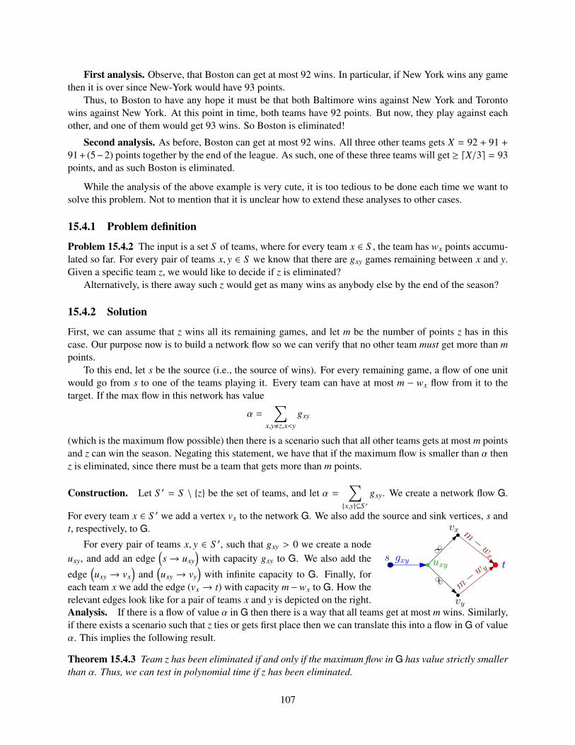
First analysis. Observe, that Boston can get at most 92 wins. In particular, if New York wins any gamethen it is over since New-York would have 93 points.

Thus, to Boston to have any hope it must be that both Baltimore wins against New York and Torontowins against New York. At this point in time, both teams have 92 points. But now, they play against eachother, and one of them would get 93 wins. So Boston is eliminated!

Second analysis. As before, Boston can get at most 92 wins. All three other teams gets X = 92 + 91 +91+ (5−2) points together by the end of the league. As such, one of these three teams will get ≥ dX/3e = 93points, and as such Boston is eliminated.

While the analysis of the above example is very cute, it is too tedious to be done each time we want tosolve this problem. Not to mention that it is unclear how to extend these analyses to other cases.

15.4.1 Problem definition

Problem 15.4.2 The input is a set S of teams, where for every team x ∈ S , the team has wx points accumu-lated so far. For every pair of teams x, y ∈ S we know that there are gxy games remaining between x and y.Given a specific team z, we would like to decide if z is eliminated?

Alternatively, is there away such z would get as many wins as anybody else by the end of the season?

15.4.2 Solution

First, we can assume that z wins all its remaining games, and let m be the number of points z has in thiscase. Our purpose now is to build a network flow so we can verify that no other team must get more than mpoints.

To this end, let s be the source (i.e., the source of wins). For every remaining game, a flow of one unitwould go from s to one of the teams playing it. Every team can have at most m − wx flow from it to thetarget. If the max flow in this network has value

α =∑

x,y,z,x<y

gxy

(which is the maximum flow possible) then there is a scenario such that all other teams gets at most m pointsand z can win the season. Negating this statement, we have that if the maximum flow is smaller than α thenz is eliminated, since there must be a team that gets more than m points.

Construction. Let S ′ = S \ z be the set of teams, and let α =∑x,y⊆S ′

gxy. We create a network flow G.

For every team x ∈ S ′ we add a vertex vx to the network G. We also add the source and sink vertices, s andt, respectively, to G. vx

vy

uxygxys

m−w

x

m− w y

∞

∞t

For every pair of teams x, y ∈ S ′, such that gxy > 0 we create a nodeuxy, and add an edge

(s→ uxy

)with capacity gxy to G. We also add the

edge(uxy → vx

)and

(uxy → vy

)with infinite capacity to G. Finally, for

each team x we add the edge (vx → t) with capacity m−wx to G. How therelevant edges look like for a pair of teams x and y is depicted on the right.Analysis. If there is a flow of value α in G then there is a way that all teams get at most m wins. Similarly,if there exists a scenario such that z ties or gets first place then we can translate this into a flow in G of valueα. This implies the following result.

Theorem 15.4.3 Team z has been eliminated if and only if the maximum flow in G has value strictly smallerthan α. Thus, we can test in polynomial time if z has been eliminated.

107

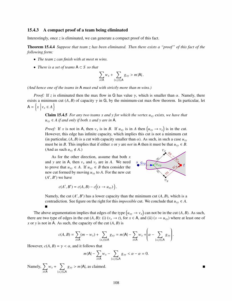
15.4.3 A compact proof of a team being eliminated

Interestingly, once z is eliminated, we can generate a compact proof of this fact.

Theorem 15.4.4 Suppose that team z has been eliminated. Then there exists a “proof” of this fact of thefollowing form:

• The team z can finish with at most m wins.

• There is a set of teams A ⊂ S so that ∑s∈A

wx +∑x,y⊆A

gxy > m |A| .

(And hence one of the teams in A must end with strictly more than m wins.)

Proof: If z is eliminated then the max flow in G has value γ, which is smaller than α. Namely, thereexists a minimum cut (A, B) of capacity γ in G, by the minimum-cut max-flow theorem. In particular, let

A =x

∣∣∣∣ vx ∈ A

Claim 15.4.5 For any two teams x and y for which the vertex uxy exists, we have thatuxy ∈ A if and only if both x and y are in A.

Proof: If x is not in A, then vx is in B. If uxy is in A then(uxy → vx

)is in the cut.

However, this edge has infinite capacity, which implies this cut is not a minimum cut(in particular, (A, B) is a cut with capacity smaller than α). As such, in such a case uxy

must be in B. This implies that if either x or y are not in A then it must be that uxy ∈ B.(And as such uxy < A.) vx

vy

uxygxys

m−w

x

m− w y

∞

∞t

As for the other direction, assume that both xand y are in A, then vx and vy are in A. We needto prove that uxy ∈ A. If uxy ∈ B then consider thenew cut formed by moving uxy to A. For the new cut(A′, B′) we have

c(A′, B′) = c(A, B) − c((s→ uxy)

).

Namely, the cut (A′, B′) has a lower capacity than the minimum cut (A, B), which is acontradiction. See figure on the right for this impossible cut. We conclude that uxy ∈ A.

The above argumentation implies that edges of the type(uxy → vx

)can not be in the cut (A, B). As such,

there are two type of edges in the cut (A, B): (i) (vx → t), for x ∈ A, and (ii) (s→ uxy) where at least one ofx or y is not in A. As such, the capacity of the cut (A, B) is

c(A, B) =∑x∈A

(m − wx) +∑x,y1A

gxy = m |A| −∑x∈A

wx +

α − ∑x,y⊆A

gxy

.However, c(A, B) = γ < α, and it follows that

m |A| −∑x∈A

wx −∑x,y⊆A

gxy < α − α = 0.

Namely,∑x∈A

wx +∑x,y⊆A

gxy > m |A|, as claimed.

108

Part IV

Min Cost Flow

109

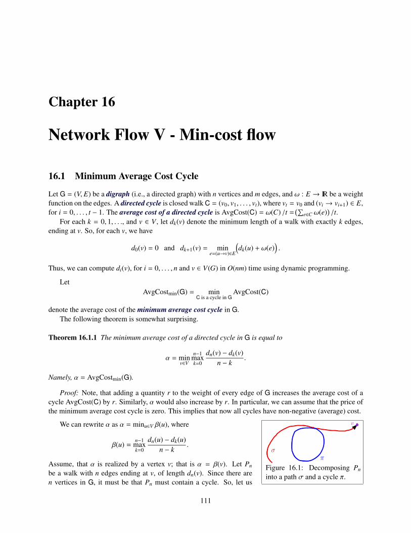
Chapter 16

Network Flow V - Min-cost flow

16.1 Minimum Average Cost Cycle

Let G = (V, E) be a digraph (i.e., a directed graph) with n vertices and m edges, and ω : E → IR be a weightfunction on the edges. A directed cycle is closed walk C = (v0, v1, . . . , vt), where vt = v0 and (vi → vi+1) ∈ E,for i = 0, . . . , t − 1. The average cost of a directed cycle is AvgCost(C) = ω(C) /t =

(∑e∈C ω(e)

)/t.

For each k = 0, 1, . . ., and v ∈ V , let dk(v) denote the minimum length of a walk with exactly k edges,ending at v. So, for each v, we have

d0(v) = 0 and dk+1(v) = mine=(u→v)∈E

(dk(u) + ω(e)

).

Thus, we can compute di(v), for i = 0, . . . , n and v ∈ V(G) in O(nm) time using dynamic programming.

LetAvgCostmin(G) = min

C is a cycle in GAvgCost(C)

denote the average cost of the minimum average cost cycle in G.The following theorem is somewhat surprising.

Theorem 16.1.1 The minimum average cost of a directed cycle in G is equal to

α = minv∈V

n−1maxk=0

dn(v) − dk(v)n − k

.

Namely, α = AvgCostmin(G).

Proof: Note, that adding a quantity r to the weight of every edge of G increases the average cost of acycle AvgCost(C) by r. Similarly, α would also increase by r. In particular, we can assume that the price ofthe minimum average cost cycle is zero. This implies that now all cycles have non-negative (average) cost.

π

v

σ

Figure 16.1: Decomposing Pn

into a path σ and a cycle π.

We can rewrite α as α = minu∈V β(u), where

β(u) =n−1

maxk=0

dn(u) − dk(u)n − k

.

Assume, that α is realized by a vertex v; that is α = β(v). Let Pn

be a walk with n edges ending at v, of length dn(v). Since there aren vertices in G, it must be that Pn must contain a cycle. So, let us

111

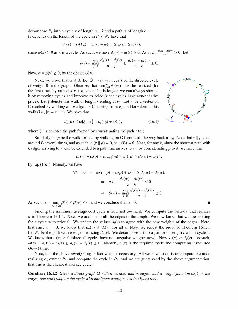
decompose Pn into a cycle π of length n − k and a path σ of length k(k depends on the length of the cycle in Pn). We have that

dn(v) = ω(Pn) = ω(π) + ω(σ) ≥ ω(σ) ≥ dk(v),

since ω(π) ≥ 0 as π is a cycle. As such, we have dn(v) − dk(v) ≥ 0. As such, dn(v)−dk(v)n−k ≥ 0. Let

β(v) =n−1

maxj=0

dn(v) − d j(v)n − j

≥dn(v) − dk(v)

n − k≥ 0.

Now, α = β(v) ≥ 0, by the choice of v.

v0ξ

wτ

ρ

C

Next, we prove that α ≤ 0. Let C = (v0, v1, . . . , vt) be the directed cycleof weight 0 in the graph. Observe, that min∞j=0 d j(v0) must be realized (forthe first time) by an index r < n, since if it is longer, we can always shortenit by removing cycles and improve its price (since cycles have non-negativeprice). Let ξ denote this walk of length r ending at v0. Let w be a vertex onC reached by walking n − r edges on C starting from v0, and let τ denote thiswalk (i.e., |τ| = n − r). We have that

dn(w) ≤ ω(ξ || τ

)= dr(v0) + ω(τ) , (16.1)

where ξ || τ denotes the path formed by concatenating the path τ to ξ.

Similarly, let ρ be the walk formed by walking on C from w all the way back to v0. Note that τ || ρ goesaround C several times, and as such, ω(τ || ρ) = 0, as ω(C) = 0. Next, for any k, since the shortest path withk edges arriving to w can be extended to a path that arrives to v0, by concatenating ρ to it, we have that

dk(w) + ω(ρ) ≥ dk+|ρ|(v0) ≥ dr(v0) ≥ dn(w) − ω(τ) ,

by Eq. (16.1). Namely, we have

∀k 0 = ω(τ || ρ) = ω(ρ) + ω(τ) ≥ dn(w) − dk(w).

⇒ ∀kdn(w) − dk(w)

n − k≤ 0

⇒ β(w) =n−1

maxk=0

dn(w) − dk(w)n − k

≤ 0.

As such, α = minv∈V(G)

β(v) ≤ β(w) ≤ 0, and we conclude that α = 0.

Finding the minimum average cost cycle is now not too hard. We compute the vertex v that realizesα in Theorem 16.1.1. Next, we add −α to all the edges in the graph. We now know that we are lookingfor a cycle with price 0. We update the values di(v) to agree with the new weights of the edges. Note,that since α = 0, we know that dn(v) ≤ di(v), for all i. Now, we repeat the proof of Theorem 16.1.1.Let Pn be the path with n edges realizing dn(v). We decompose it into a path π of length k and a cycle τ.We know that ω(τ) ≥ 0 (since all cycles have non-negative weights now). Now, ω(π) ≥ dk(v). As such,ω(τ) = dn(v) − ω(π) ≤ dn(v) − dk(v) ≤ 0. Namely, ω(τ) is the required cycle and computing it requiredO(nm) time.

Note, that the above reweighting in fact was not necessary. All we have to do is to compute the noderealizing α, extract Pn, and compute the cycle in Pn, and we are guaranteed by the above argumentation,that this is the cheapest average cycle.

Corollary 16.1.2 Given a direct graph G with n vertices and m edges, and a weight function ω(·) on theedges, one can compute the cycle with minimum average cost in O(nm) time.

112

16.2 Potentials

In general computing the shortest path in a graph that have negative weights is harder than just using theDijkstra algorithm (that works only for graphs with non-negative weights on its edges). One can use Fordalgorithm in this case, but it considerably slower (i.e., it takes O(mn) time). We next present a case whereone can still use Dijkstra algorithm, with slight modifications.

The following is only required in the analysis of the minimum-cost flow algorithm we present later inthis chapter. We describe it here in full detail since its simple and interesting.

For a directed graph G = (V, E) with weight w(·) on the edges, let dω(s, t) denote the length of theshortest path between s and t in G under the weight function w. Note, that w might assign negative weightsto edges in G.

A potential p(·) is a function that assigns a real value to each vertex of G, such that if e = (u→ v) ∈ Gthen w(e) ≥ p(v) − p(u).

Lemma 16.2.1 (i) There exists a potential p(·) for G if and only if G has no negative cycles (with respect tow(·)).

(ii) Given a potential function p(·), for an edge e = (u→ v) ∈ E(G), let `(e) = w(e) − p(v) + p(u). Then`(·) is non-negative for the edges in the graph and for any pair of vertices s, t ∈ V(G), we have that theshortest path π realizing d`(s, t) also realizes dω(s, t).

(iii) Given G and a potential function p(·), one can compute the shortest path from s to all the verticesof G in O(n log n + m) time, where G has n vertices and m edges

Proof: (i) Consider a cycle C, and assume there is a potential p(·) for G, and observe that

w(C) =∑

(u→v)∈E(C)

w(e) ≥∑

(u→v)∈E(C)

(p(v) − p(u)) = 0,

as required.For a vertex v ∈ V(G), let p(v) denote the shortest walk that ends at v in G. We claim that p(v) is a

potential. Since G does not have negative cycles, the quantity p(v) is well defined. Observe that p(v) ≤p(u)+w(u→ v) since we can always continue a walk to u into v by traversing (u→ v). Thus, p(v)− p(u) ≤w(u→ v), as required.

(ii) Since `(e) = w(e)− p(v)+ p(u) we have that w(e) ≥ p(v)− p(u) since p(·) is a potential function. Assuch w(e) − p(v) + p(u) ≥ 0, as required.

As for the other claim, observe that for any path π in G starting at s and ending at t we have that

`(π) =∑

e=(u→v)∈π

(w(e) − p(v) + p(u)) = w(π) + p(s) − p(t),

which implies that d`(s, t) = dω(s, t) + p(s) − p(t). Implying the claim.(iii) Just use the Dijkstra algorithm on the distances defined by `(·). The shortest paths are preserved

under this distance by (iii), and this distance function is always positive.

16.3 Minimum cost flow

Given a network flow G = (V, E) with source s and sink t, capacities c(·) on the edges, a real number φ, anda cost function κ(·) on the edges. The cost of a flow f is defined to be

cost(f) =∑e∈E

κ(e) ∗ f(e).

113

The minimum-cost s-t flow problem ask to find the flow f that minimizes the cost and has value φ.It would be easier to look on the problem of minimum-cost circulation problem. Here, we are given

instead of φ a lower-bound `(·) on the flow on every edge (and the regular upper bound c(·) on the capacitiesof the edges). All the flow coming into a node must leave this node. It is easy to verify that if we cansolve the minimum-cost circulation problem, then we can solve the min-cost flow problem. Thus, we willconcentrate on the min-cost circulation problem.

An important technicality is that all the circulations we discuss here have zero demands on the vertices.As such, a circulation can be conceptually considered to be a flow going around in cycles in the graphwithout ever stopping. In particular, for these circulations, the conservation of flow property should hold forall the vertices in the graph.

The residual graph of f is the graph Gf = (V, Ef) where

Ef =

e = (u→ v) ∈ V × V

∣∣∣∣ f(e) < c(e) or f(e−1

)> `

(e−1

).

where e−1 = (v→ u) if e = (u→ v). Note, that the definition of the residual network takes into account thelower-bound on the capacity of the edges.

Assumption 16.3.1 To simplify the exposition, we will assume that if (u→ v) ∈ E(G) then (v→ u) < E(G),for all u, v ∈ V(G). This can be easily enforced by introducing a vertex in the middle of every edge of G.

Since we are more concerned with solving the problem at hand in polynomial time, than the exactcomplexity. Note, that our discussion can be extended to handle the slightly more general case, with a bit ofcare.

We extend the cost function to be anti-symmetric; namely,

∀ (u→ v) ∈ Ef κ(

(u→ v))= −κ

((v→ u)

).

Consider a directed cycle C in Gf. For an edge e = (u→ v) ∈ E, we define

χC(e) =

1 e ∈ C−1 e−1 = (v→ u) ∈ C0 otherwise;

that is, we pay 1 if e is in C and −1 if we travel e in the “wrong” direction.The cost of a directed cycle C in Gf is defined as

κ(C) =∑e∈C

κ (e) .

We will refer to a circulation that comply with the capacity and lower-bounds constraints as being valid.A function that just comply with the conservation property (i.e., all incoming flow into a vertex leaves it), isa weak circulation. In particular, a weak circulation might not comply with the capacity and lower boundsconstraints of the given instance, and as such is not a valid circulation.

We need the following easy technical lemmas.

Lemma 16.3.2 Let f and g be two valid circulations in G = (V, E). Consider the function h = g − f. Then,h is a weak circulation, and if h(u→ v) > 0 then the edge (u→ v) ∈ Gf.

114

Proof: The fact that h is a circulation is trivial, as it is the difference between two circulations, and as suchthe same amount of flow that comes into a vertex leaves it, and thus it is a circulation. (Note, that h mightnot be a valid circulation, since it might not comply with the lower-bounds on the edges.)

Observe, that if h(u→ v) is negative, then h(v→ u) = −h(u→ v) by the anti-symmetry of f and g,which implies the same property holds for h.

Consider an arbitrary edge e = (u→ v) such that h(u→ v) > 0.There are two possibilities. First, if e = (u→ v) ∈ E, and f(e) < c(e), then the claim trivially holds, since

then e ∈ Gf. Thus, consider the case when f(e) = c(e), but then h(e) = g(e) − f(e) ≤ 0. Which contradictsour assumption that h(u→ v) > 0.

The second possibility, is that e = (u→ v) < E. But then e−1 = (v→ u) must be in E, and it holds0 > h

(e−1

)= g

(e−1

)− f

(e−1

). Implying that f

(e−1

)> g

(e−1

)≥ `

(e−1

). Namely, there is a flow by f in G

going in the direction of e−1 which larger than the lower bound. Since we can return this flow in the otherdirection, it must be that e ∈ Gf.

Lemma 16.3.3 Let f be a circulation in a graph G. Then, f can be decomposed into at most m cycles,C1, . . . ,Cm, such that, for any e ∈ E(G), we have

f(e) =t∑

i=1

λi · χCi(e),

where λ1, . . . , λt > 0 and t ≤ m, where m is the number of edges in G.

Proof: Since f is a circulation, and the amount of flow into a node is equal to the amount of flow leavingthe node, it follows that as long as f not zero, one can find a cycle in f. Indeed, start with a vertex whichhas non-zero amount of flow into it, and walk on an adjacent edge that has positive flow on it. Repeat thisprocess, till you visit a vertex that was already visited. Now, extract the cycle contained in this walk.

Let C1 be such a cycle, and observe that every edge of C1 has positive flow on it, let λ1 be the smallestamount of flow on any edge of C1, and let e1 denote this edge. Consider the new flow g = f − λ1 · χC1 .Clearly, g has zero flow on e1, and it is a circulation. Thus, we can remove e1 from G, and let H denote thenew graph. By induction, applied to g on H, the flow g can be decomposed into m − 1 cycles with positivecoefficients. Putting these cycles together with λ1 and C1 implies the claim.

Theorem 16.3.4 A flow f is a minimum cost feasible circulation if and only if each directed cycle of Gf hasnonnegative cost.

Proof: Let C be a negative cost cycle in Gf. Then, we can circulate more flow on C and get a flow withsmaller price. In particular, let ε > 0 be a sufficiently small constant, such that g = f+ε∗χC is still a feasiblecirculation (observe, that since the edges of C are Gf, all of them have residual capacity that can be used tothis end). Now, we have that

cost(g) = cost(f) +∑e∈C

κ(e) ∗ ε = cost(f) + ε ∗∑e∈C

κ(e) = cost(f) + ε ∗ κ(C) < cost(f),

since κ(C) < 0, which is a contradiction to the minimality of f.As for the other direction, assume that all the cycles in Gf have non-negative cost. Then, let g be any

feasible circulation. Consider the circulation h = g − f. By Lemma 16.3.2, all the edges used by h are in Gf,and by Lemma 16.3.3 we can find t ≤ |E(Gf)| cycles C1, . . . ,Ct in Gf, and coefficients λ1, . . . , λt, such that

h(e) =t∑

i=1

λiχCi(e).

115

We have that

cost(g) − cost(f) = cost(h) = cost

t∑i=1

λiχCi

= t∑i=1

λicost(χCi

)=

t∑i=1

λiκ (Ci) ≥ 0,

as κ(Ci) ≥ 0, since there are no negative cycles in Gf. This implies that cost(g) ≥ cost(f). Namely, f is aminimum-cost circulation.

16.4 A Strongly Polynomial Time Algorithm for Min-Cost Flow

The algorithm would start from a feasible circulation f. We know how to compute such a flow f using thestandard max-flow algorithm. At each iteration, it would find the cycle C of minimum average cost cycle inGf (using the algorithm of Section 16.1). If the cost of C is non-negative, we are done since we had arrivedto the minimum cost circulation, by Theorem 16.3.4.

Otherwise, we circulate as much flow as possible along C (without violating the lower-bound constraintsand capacity constraints), and reduce the price of the flow f. By Corollary 16.1.2, we can compute such acycle in O(mn) time. Since the cost of the flow is monotonically decreasing the algorithm would terminateif all the number involved are integers. But we will show in fact that his algorithm performs a polynomialnumber of iterations in n and m.

It is striking how simple is this algorithm, and the fact that it works in polynomial time. The analysis issomewhat more painful.

16.5 Analysis of the Algorithm

f, g, h, i Flows or circulationsGf The residual graph for fc(e) The capacity of the flow on e`(e) The lower-bound (i.e., demand) on the flow on ecost(f) The overall cost of the flow fκ(e) The cost of sending one unit of flow on eψ(e) The reduced cost of e

Figure 16.2: Notation used.

To analyze the above algorithm, letfi be the flow in the beginning of the ithiteration. Let Ci be the cycle used in theith iteration. For a flow f, let Cf the min-imum average-length cycle of Gf, andlet µ(f) = κ(Cf)/ |Cf| denote the average“cost” per edge of Cf.

The following lemma, states that weare making “progress” in each iterationof the algorithm.

Lemma 16.5.1 Let f be a flow, and let g the flow resulting from applying the cycle C = Cf to it. Then,µ(g) ≥ µ(f).

Proof: Assume for the sake of contradiction, that µ(g) < µ(f). Namely, we have

κ(Cg)∣∣∣Cg∣∣∣ <

κ(Cf)|Cf|

. (16.2)

Now, the only difference between Gf and Gg are the edges of Cf. In particular, some edges of Cf mightdisappear from Gg, as they are being used in g to their full capacity. Also, all the edges in the oppositedirection to Cf will be present in Gg.

Now, Cg must use at least one of the new edges in Gg, since otherwise this would contradict the mini-mality of Cf (i.e., we could use Cg in Gf and get a cheaper average cost cycle than Cf). Let U be the set of

116

new edges of Gg that are being used by Cg and are not present in Gf. Let U−1 =

e−1

∣∣∣∣ e ∈ U. Clearly, all

the edges of U−1 appear in Cf.Now, consider the cycle π = Cf ∪ Cg. We have that the average of π is

α =κ(Cf) + κ(Cg)

|Cf| +∣∣∣Cg

∣∣∣ < max

κ(Cg)∣∣∣Cg∣∣∣ , κ(Cf)|Cf|

= µ(f) ,

by Eq. (16.2). We can write π is a union of k edge-disjoint cycles σ1, . . . , σk and some 2-cycles. A 2-cycleis formed by a pair of edges e and e−1 where e ∈ U and e−1 ∈ U−1. Clearly, the cost of these 2-cycles iszero. Thus, since the cycles σ1, . . . , σk have no edges in U, it follows that they are all contained in Gf. Wehave

κ(Cf) + κ(Cg

)=

∑i

κ(σi) + 0.

Thus, there is some non-negative integer constant c, such that

α =κ(Cf) + κ(Cg)

|Cf| +∣∣∣Cg

∣∣∣ =∑

i κ(σi)c +

∑i |σi|

≥

∑i κ(σi)∑i |σi|

,

since α is negative (since α < µ(f) < 0 as otherwise the algorithm would had already terminated). Namely,µ(f) >

(∑i κ(σi)

)/(∑

i |σi|). Which implies that there is a cycle σr, such that µ(f) > κ(σr)/|σr | and this cycle

is contained in Gf. But this is a contradiction to the minimality of µ(f).

16.5.1 Reduced cost induced by a circulation

Conceptually, consider the function µ(f) to be a potential function that increases as the algorithm progresses.To make further progress in our analysis, it would be convenient to consider a reweighting of the edges ofG, in such a way that preserves the weights of cycles.

Given a circulation f, we are going to define a different cost function on the edges which is induced by f.To begin with, let β(u→ v) = κ(u→ v) − µ(f). Note, that under the cost function α, the cheapest cycle hasprice 0 in G (since the average cost of an edge in the cheapest average cycle has price zero). Namely, G hasno negative cycles under β. Thus, for every vertex v ∈ V(G), let d(v) denote the length of the shortest walkthat ends at v. The function d(v) is a potential in G, by Lemma 16.2.1, and as such

d(v) − d(u) ≤ β(u→ v) = κ(u→ v) − µ(f) . (16.3)

Next, let the reduced cost of (u→ v) (in relation to f) be

ψ(u→ v) = κ(u→ v) + d(u) − d(v).

In particular, Eq. (16.3) implies that

∀ (u→ v) ∈ E(Gf) ψ(u→ v) = κ(u→ v) + d(u) − d(v) ≥ µ(f) . (16.4)

Namely, the reduced cost of any edge (u→ v) is at least µ(f).Note that ψ(v→ u) = κ(v→ u) + d(v) − d(u) = −κ(u→ v) + d(v) − d(u) = −ψ(u→ v) (i.e., it is anti-

symmetric). Also, for any cycle C in G, we have that κ(C) = ψ(C), since the contribution of the potentiald(·) cancels out.

The idea is that now we think about the algorithm as running with the reduced cost instead of the regularcosts. Since the costs of cycles under the original cost and the reduced costs are the same, negative cyclesare negative in both costs. The advantage is that the reduced cost is more useful for our purposes.

117

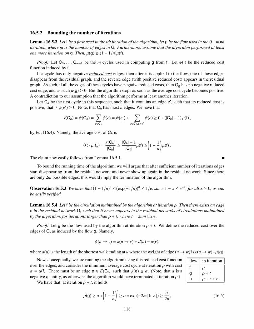
16.5.2 Bounding the number of iterations

Lemma 16.5.2 Let f be a flow used in the ith iteration of the algorithm, let g be the flow used in the (i+m)thiteration, where m is the number of edges in G. Furthermore, assume that the algorithm performed at leastone more iteration on g. Then, µ(g) ≥ (1 − 1/n)µ(f).

Proof: Let C0, . . . ,Cm−1 be the m cycles used in computing g from f. Let ψ(·) be the reduced costfunction induced by f.

If a cycle has only negative reduced cost edges, then after it is applied to the flow, one of these edgesdisappear from the residual graph, and the reverse edge (with positive reduced cost) appears in the residualgraph. As such, if all the edges of these cycles have negative reduced costs, then Gg has no negative reducedcost edge, and as such µ(g) ≥ 0. But the algorithm stops as soon as the average cost cycle becomes positive.A contradiction to our assumption that the algorithm performs at least another iteration.

Let Ch be the first cycle in this sequence, such that it contains an edge e′, such that its reduced cost ispositive; that is ψ(e′) ≥ 0. Note, that Ch has most n edges. We have that

κ(Ch) = ψ(Ch) =∑e∈Ch

ψ(e) = ψ(e′)+

∑e∈Ch,e,e′

ψ(e) ≥ 0 +(|Ch| − 1) µ(f) ,

by Eq. (16.4). Namely, the average cost of Ch is

0 > µ(fh) =κ(Ch)|Ch|

≥|Ch| − 1|Ch|

µ(f) ≥(1 −

1n

)µ(f) .

The claim now easily follows from Lemma 16.5.1.

To bound the running time of the algorithm, we will argue that after sufficient number of iterations edgesstart disappearing from the residual network and never show up again in the residual network. Since thereare only 2m possible edges, this would imply the termination of the algorithm.

Observation 16.5.3 We have that (1 − 1/n)n ≤(exp(−1/n)

)n≤ 1/e, since 1 − x ≤ e−x, for all x ≥ 0, as can

be easily verified.

Lemma 16.5.4 Let f be the circulation maintained by the algorithm at iteration ρ. Then there exists an edgee in the residual network Gf such that it never appears in the residual networks of circulations maintainedby the algorithm, for iterations larger than ρ + t, where t = 2nm dln ne.

Proof: Let g be the flow used by the algorithm at iteration ρ + t. We define the reduced cost over theedges of G, as induced by the flow g. Namely,

ψ(u→ v) = κ(u→ v) + d(u) − d(v),

where d(u) is the length of the shortest walk ending at u where the weight of edge (u→ w) is κ(u→ w)−µ(g).

flow in iterationf ρ

g ρ + th ρ + t + τ

Now, conceptually, we are running the algorithm using this reduced cost functionover the edges, and consider the minimum average cost cycle at iteration ρ with costα = µ(f). There must be an edge e ∈ E(Gf), such that ψ(e) ≤ α. (Note, that α is anegative quantity, as otherwise the algorithm would have terminated at iteration ρ.)

We have that, at iteration ρ + t, it holds

µ(g) ≥ α ∗(1 −

1n

)t

≥ α ∗ exp(−2m dln ne) ≥α

2n, (16.5)

118

by Lemma 16.5.2 and Observation 16.5.3 and since α < 0. On the other hand, by Eq. (16.4), we know thatfor all the edges f in E

(Gg

), it holds ψ(f) ≥ µ(g) ≥ α/2n. As such, e can not be an edge of Gg since ψ(e) ≤ α.

Namely, it must be that g(e) = c(e).So, assume that at a later iteration, say ρ + t + τ, the edge e reappeared in the residual graph. Let h be

the flow at the (ρ + t + τ)th iteration, and let Gh be the residual graph. It must be that h(e) < c(e) = g(e).Now, consider the circulation i = g−h. It has a positive flow on the edge e, since i(e) = g(e)−h(e) > 0. In

particular, there is a directed cycle C of positive flow of i in Gi that includes e, as implied by Lemma 16.3.3.Note, that Lemma 16.3.2 implies that C is also a cycle of Gh.

Now, the edges of C−1 are present in Gg. To see that, observe that for every edge g ∈ C, we have that0 < i(g) = g(g) − h(g) ≤ g(g) − `(g). Namely, g(g) > `(g) and as such g−1 ∈ E

(Gg

). As such, by Eq. (16.4),

we have ψ(g−1

)≥ µ(g). This implies

∀g ∈ C ψ(g) = −ψ(g−1

)≤ −µ(g) ≤ −

α

2n,

by Eq. (16.5). Since C is a cycle of Gh, we have

κ(C) = ψ(C) = ψ(e) + ψ(C \ e) ≤ α + (|C| − 1) ·(−α

2n

)<α

2.

Namely, the average cost of the cycle C, which is present in Gh, is κ(C)/ |C| < α/(2n).On the other hand, the minimum average cost cycle in Gh has average price µ(h) ≥ µ(g) ≥ α

2n , byLemma 16.5.1. A contradiction, since we found a cycle C in Gh which is cheaper.

We are now ready for the “kill” – since one edge disappears forever every O(mn log n) iterations, itfollows that after O(m2n log n) iterations the algorithm terminates. Every iteration takes O(mn) time, byCorollary 16.1.2. Putting everything together, we get the following.

Theorem 16.5.5 Given a digraph G with n vertices and m edges, lower bound and upper bound on the flowof each edge, and a cost associated with each edge, then one can compute a valid circulation of minimum-cost in O(m3n2 log n) time.


The minimum average cost cycle algorithm, of Section 16.1, is due to Karp [Kar78].The description here follows very roughly the description of [Sch04]. The first strongly polynomial

time algorithm for minimum-cost circulation is due to Éva Tardos [Tar85]. The algorithm we show is animproved version due to Andrew Goldberg and Robert Tarjan [GT89]. Initial research on this problem canbe traced back to the 1940s, so it took almost fifty years to find a satisfactory solution to this problem.

119

120

Part V

Min Cost Flow

121

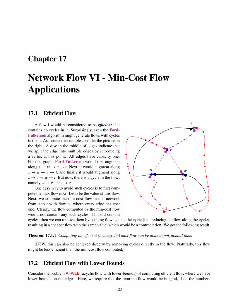
Chapter 17

Network Flow VI - Min-Cost FlowApplications

17.1 Efficient Flow

s

t

u

v

w

A flow f would be considered to be efficient if itcontains no cycles in it. Surprisingly, even the Ford-Fulkerson algorithm might generate flows with cyclesin them. As a concrete example consider the picture onthe right. A disc in the middle of edges indicate thatwe split the edge into multiple edges by introducinga vertex at this point. All edges have capacity one.For this graph, Ford-Fulkerson would first augmentalong s → w → u → t. Next, it would augment alongs → u → v → t, and finally it would augment alongs→ v→ w→ t. But now, there is a cycle in the flow;namely, u→ v→ w→ u.

One easy way to avoid such cycles is to first com-pute the max flow in G. Let α be the value of this flow.Next, we compute the min-cost flow in this networkfrom s to t with flow α, where every edge has costone. Clearly, the flow computed by the min-cost flowwould not contain any such cycles. If it did containcycles, then we can remove them by pushing flow against the cycle (i.e., reducing the flow along the cycle),resulting in a cheaper flow with the same value, which would be a contradiction. We got the following result.

Theorem 17.1.1 Computing an efficient (i.e., acyclic) max-flow can be done in polynomial time.

(BTW, this can also be achieved directly by removing cycles directly in the flow. Naturally, this flowmight be less efficient than the min-cost flow computed.)

17.2 Efficient Flow with Lower Bounds

Consider the problem AFWLB (acyclic flow with lower-bounds) of computing efficient flow, where we havelower bounds on the edges. Here, we require that the returned flow would be integral, if all the numbers

123

involved are integers. Surprisingly, this problem which looks like very similar to the problems we knowhow to solve efficiently is NP-C. Indeed, consider the following problem.

Problem: Hamiltonian Path

Instance: A directed graph G and two vertices s and t.Question: Is there a Hamiltonian path (i.e., a path visiting every vertex exactly once)in G starting at s and ending at t?

It is easy to verify that Hamiltonian Path is NP-C . We reduce this problem to AFWLB byreplacing each vertex of G with two vertices and a direct edge in between them (except for the source vertexs and the sink vertex t). We set the lower-bound and capacity of each such edge to 1. Let H denote theresulting graph.

Consider now acyclic flow in H of capacity 1 from s to t which is integral. Its 0/1-flow, and as such itdefines a path that visits all the special edges we created. In particular, it corresponds to a path in the originalgraph that starts at s, visits all the vertices of G and ends up at t. Namely, if we can compute an integralacyclic flow with lower-bounds in H in polynomial time, then we can solve Hamiltonian path in polynomialtime. Thus, AFWLB is NP-H. flow in the new graph

Theorem 17.2.1 Computing an efficient (i.e., acyclic) max-flow with lower-bounds is NP-H (where theflow must be integral). The related decision problem (of whether such a flow exist) is NP-C.

17.3 Shortest Edge-Disjoint Paths

Let G be a directed graph. We would like to compute k-edge disjoint paths between vertices s and t in thegraph. We know how to do it using network flow. Interestingly, we can find the shortest k-edge disjointpaths using min-cost flow. Here, we assign cost 1 for every edge, and capacity 1 for every edge. Clearly, themin-cost flow in this graph with value k, corresponds to a set of k edge disjoint paths, such that their totallength is minimized.

17.4 Covering by Cycles

Given a direct graph G, we would like to cover all its vertices by a set of cycles which are vertex disjoint. Thiscan be done again using min-cost flow. Indeed, replace every vertex u in G by an edge (u′ → u′′). Whereall the incoming edges to u are connected to u′ and all the outgoing edges from u are now starting from u′′.Let H denote the resulting graph. All the new edges in the graph have a lower bound and capacity 1, and allthe other edges have no lower bound, but their capacity is 1. We compute the minimum cost circulation inH. Clearly, this corresponds to a collection of cycles in G covering all the vertices of minimum cost.

Theorem 17.4.1 Given a directed graph G and costs on the edges, one can compute a cover of G by acollection of vertex disjoint cycles, such that the total cost of the cycles is minimized.

17.5 Minimum weight bipartite matching

Verify that you know to do this — its a natural question for the exam.

124

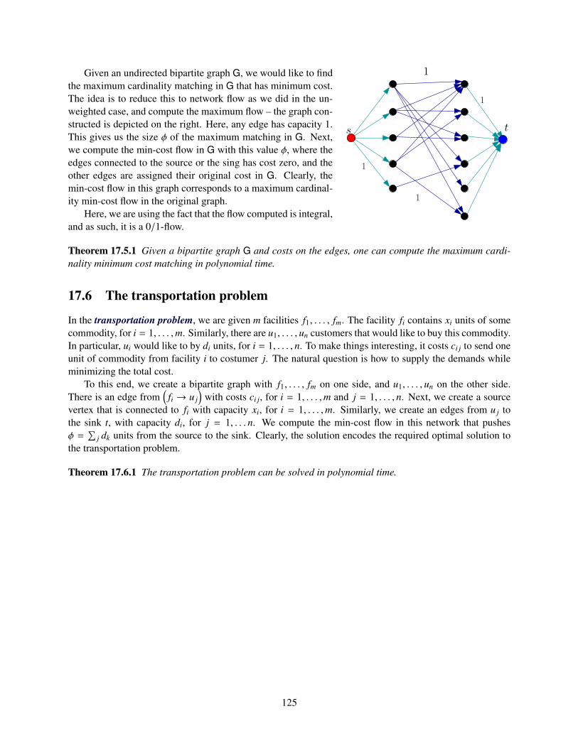
ts

1

1

1

1

Given an undirected bipartite graph G, we would like to findthe maximum cardinality matching in G that has minimum cost.The idea is to reduce this to network flow as we did in the un-weighted case, and compute the maximum flow – the graph con-structed is depicted on the right. Here, any edge has capacity 1.This gives us the size φ of the maximum matching in G. Next,we compute the min-cost flow in G with this value φ, where theedges connected to the source or the sing has cost zero, and theother edges are assigned their original cost in G. Clearly, themin-cost flow in this graph corresponds to a maximum cardinal-ity min-cost flow in the original graph.

Here, we are using the fact that the flow computed is integral,and as such, it is a 0/1-flow.

Theorem 17.5.1 Given a bipartite graph G and costs on the edges, one can compute the maximum cardi-nality minimum cost matching in polynomial time.

17.6 The transportation problem

In the transportation problem, we are given m facilities f1, . . . , fm. The facility fi contains xi units of somecommodity, for i = 1, . . . ,m. Similarly, there are u1, . . . , un customers that would like to buy this commodity.In particular, ui would like to by di units, for i = 1, . . . , n. To make things interesting, it costs ci j to send oneunit of commodity from facility i to costumer j. The natural question is how to supply the demands whileminimizing the total cost.

To this end, we create a bipartite graph with f1, . . . , fm on one side, and u1, . . . , un on the other side.There is an edge from

(fi → u j

)with costs ci j, for i = 1, . . . ,m and j = 1, . . . , n. Next, we create a source

vertex that is connected to fi with capacity xi, for i = 1, . . . ,m. Similarly, we create an edges from u j tothe sink t, with capacity di, for j = 1, . . . n. We compute the min-cost flow in this network that pushesφ =

∑j dk units from the source to the sink. Clearly, the solution encodes the required optimal solution to

the transportation problem.

Theorem 17.6.1 The transportation problem can be solved in polynomial time.

125

126

Part VI

Fast Fourier Transform

127

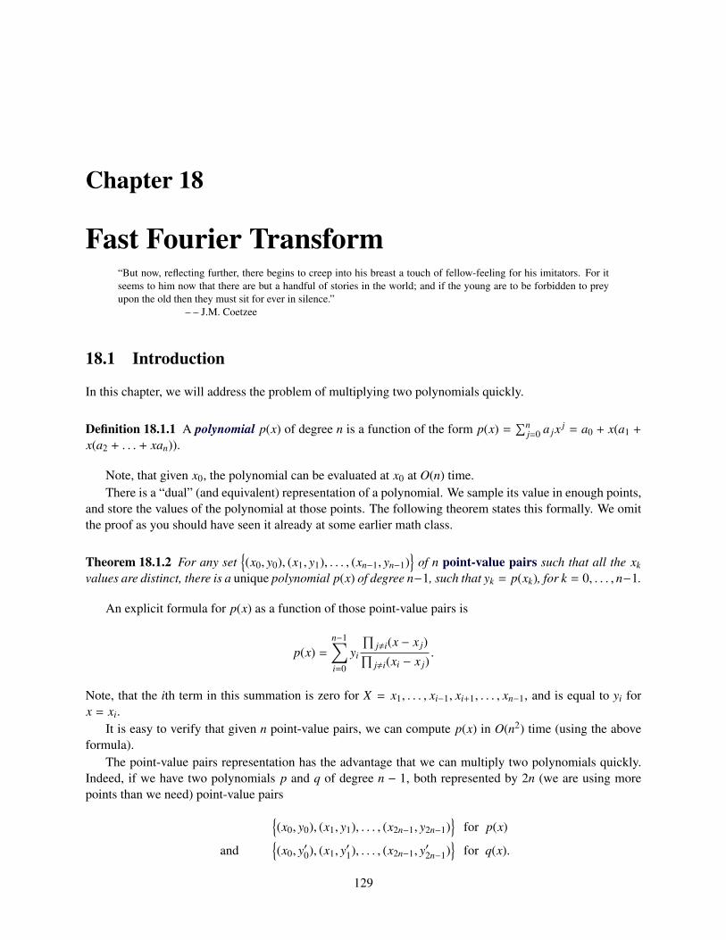
Chapter 18

Fast Fourier Transform“But now, reflecting further, there begins to creep into his breast a touch of fellow-feeling for his imitators. For itseems to him now that there are but a handful of stories in the world; and if the young are to be forbidden to preyupon the old then they must sit for ever in silence.”

– – J.M. Coetzee

18.1 Introduction

In this chapter, we will address the problem of multiplying two polynomials quickly.

Definition 18.1.1 A polynomial p(x) of degree n is a function of the form p(x) =∑n

j=0 a jx j = a0 + x(a1 +

x(a2 + . . . + xan)).

Note, that given x0, the polynomial can be evaluated at x0 at O(n) time.There is a “dual” (and equivalent) representation of a polynomial. We sample its value in enough points,

and store the values of the polynomial at those points. The following theorem states this formally. We omitthe proof as you should have seen it already at some earlier math class.

Theorem 18.1.2 For any set(x0, y0), (x1, y1), . . . , (xn−1, yn−1)

of n point-value pairs such that all the xk

values are distinct, there is a unique polynomial p(x) of degree n−1, such that yk = p(xk), for k = 0, . . . , n−1.

An explicit formula for p(x) as a function of those point-value pairs is

p(x) =n−1∑i=0

yi

∏j,i(x − x j)∏j,i(xi − x j)

.

Note, that the ith term in this summation is zero for X = x1, . . . , xi−1, xi+1, . . . , xn−1, and is equal to yi forx = xi.

It is easy to verify that given n point-value pairs, we can compute p(x) in O(n2) time (using the aboveformula).

The point-value pairs representation has the advantage that we can multiply two polynomials quickly.Indeed, if we have two polynomials p and q of degree n − 1, both represented by 2n (we are using morepoints than we need) point-value pairs

(x0, y0), (x1, y1), . . . , (x2n−1, y2n−1)

for p(x)

and(x0, y′0), (x1, y′1), . . . , (x2n−1, y′2n−1)

for q(x).

129

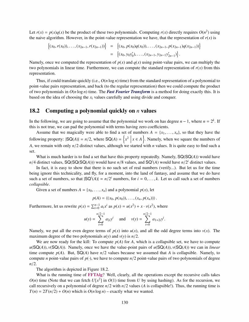
Let r(x) = p(x)q(x) be the product of these two polynomials. Computing r(x) directly requires O(n2) usingthe naive algorithm. However, in the point-value representation we have, that the representation of r(x) is

(x0, r(x0)), . . . , (x2n−1, r(x2n−1))=

(x0, p(x0)q(x0)), . . . , (x2n−1, p(x2n−1)q(x2n−1))

=

(x0, y0y′0), . . . , (x2n−1, y2n−1y′2n−1)

.

Namely, once we computed the representation of p(x) and q(x) using point-value pairs, we can multiply thetwo polynomials in linear time. Furthermore, we can compute the standard representation of r(x) from thisrepresentation.

Thus, if could translate quickly (i.e., O(n log n) time) from the standard representation of a polynomial topoint-value pairs representation, and back (to the regular representation) then we could compute the productof two polynomials in O(n log n) time. The Fast Fourier Transform is a method for doing exactly this. It isbased on the idea of choosing the xi values carefully and using divide and conquer.

18.2 Computing a polynomial quickly on n values

In the following, we are going to assume that the polynomial we work on has degree n − 1, where n = 2k. Ifthis is not true, we can pad the polynomial with terms having zero coefficients.

Assume that we magically were able to find a set of numbers A = x1, . . . , xn, so that they have the

following property: |SQ(A)| = n/2, where SQ(A) =x2

∣∣∣∣ x ∈ A. Namely, when we square the numbers of

A, we remain with only n/2 distinct values, although we started with n values. It is quite easy to find such aset.

What is much harder is to find a set that have this property repeatedly. Namely, SQ(SQ(A)) would haven/4 distinct values, SQ(SQ(SQ(A))) would have n/8 values, and SQi(A) would have n/2i distinct values.

In fact, it is easy to show that there is no such set of real numbers (verify...). But let us for the timebeing ignore this technicality, and fly, for a moment, into the land of fantasy, and assume that we do havesuch a set of numbers, so that |SQi(A)| = n/2i numbers, for i = 0, . . . , k. Let us call such a set of numberscollapsible.

Given a set of numbers A = x0, . . . , xn and a polynomial p(x), let

p(A) = 〈(x0, p(x0)), . . . , (xn, p(xn))〉 .

Furthermore, let us rewrite p(x) =∑n−1

i=0 aixi as p(x) = u(x2) + x · v(x2), where

u(y) =n/2−1∑

i=0

a2iyi and v(y) =n/2−1∑

i=0

a1+2iyi.

Namely, we put all the even degree terms of p(x) into u(x), and all the odd degree terms into v(x). Themaximum degree of the two polynomials u(y) and v(y) is n/2.

We are now ready for the kill: To compute p(A) for A, which is a collapsible set, we have to computeu(SQ(A)), v(SQ(A)). Namely, once we have the value-point pairs of u(SQ(A)), v(SQ(A)) we can in lineartime compute p(A). But, SQ(A) have n/2 values because we assumed that A is collapsible. Namely, tocompute n point-value pairs of p(·), we have to compute n/2 point-value pairs of two polynomials of degreen/2.

The algorithm is depicted in Figure 18.2.What is the running time of FFTAlg? Well, clearly, all the operations except the recursive calls takes

O(n) time (Note that we can fetch U[x2] in O(1) time from U by using hashing). As for the recursion, wecall recursively on a polynomial of degree n/2 with n/2 values (A is collapsible!). Thus, the running time isT (n) = 2T (n/2) + O(n) which is O(n log n) – exactly what we wanted.

130

Algorithm FFTAlg (p, X)input: p(x): A polynomial of degree n: p(x) =

∑n−1i=0 aixi

X: A collapsible set of n elements.output: p(X)

beginu(y) =

∑n/2−1i=0 a2iyi

v(y) =∑n/2−1

i=0 a1+2iyi.

Y = SQ(A) =x2

∣∣∣∣ x ∈ A.

U =FFTAlg(u, Y) /* U = u(Y) */V =FFTAlg (v, Y) /* V = v(Y) */

Out ← ∅for x ∈ A do/* p(x) = u(x2) + x ∗ v(x2) *//* U[x2] is the value u(x2) */(x, p(x))←

(x,U[x2] + x · V[x2]

)Out ← Out ∪ (x, p(x))

return Outend

18.2.1 Generating Collapsible Sets

Nice! But how do we resolve this “technicality” of not having collapsible set? It turns out that if workover the complex numbers instead of over the real numbers, then generating collapsible sets is quite easy.Describing complex numbers is outside the scope of this writeup, and we assume that you already haveencountered them before. Everything you can do over the real numbers you can do over the complexnumbers, and much more (complex numbers are your friend). In particular, let γ denote a nth root of unity.There are n such roots, and let γ j(n) denote the jth root. In particular, let

γ j(n) = cos((2π j)/n) + i sin((2π j)/n) = γ j.

Let A(n) = γ0(n), . . . , γn−1(n). It is easy to verify that |SQ(A(n))| has exactly n/2 elements. In fact,SQ(A(n)) = A(n/2), as can be easily verified. Namely, if we pick n to be a power of 2, then A(n) is therequired collapsible set.

Theorem 18.2.1 Given polynomial p(x) of degree n, where n is a power of two, then we can compute p(X)in O(n log n) time, where X = A(n) is the set of n different powers of the nth root of unity over the complexnumbers.

We can now multiply two polynomials quickly by transforming them to the point-value pairs repre-sentation over the nth root of unity, but we still have to transform this representation back to the regularrepresentation.

131

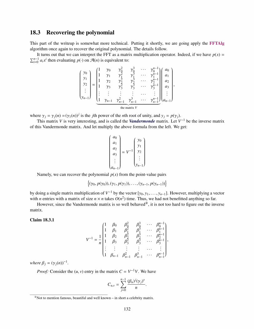
18.3 Recovering the polynomial

This part of the writeup is somewhat more technical. Putting it shortly, we are going apply the FFTAlgalgorithm once again to recover the original polynomial. The details follow.

It turns out that we can interpret the FFT as a matrix multiplication operator. Indeed, if we have p(x) =∑n−1i=0 aixi then evaluating p(·) onA(n) is equivalent to:

y0y1y2...

yn−1

=

1 γ0 γ20 γ3

0 · · · γn−10

1 γ1 γ21 γ3

1 · · · γn−11

1 γ2 γ22 γ3

2 · · · γn−12

1 γ3 γ23 γ3

3 · · · γn−13

......

...... · · ·

...

1 γn−1 γ2n−1 γ3

n−1 · · · γn−1n−1

︸︷︷︸the matrix V

a0a1a2a3...

an−1

,

where γ j = γ j(n) = (γ1(n)) j is the jth power of the nth root of unity, and y j = p(γ j).This matrix V is very interesting, and is called the Vandermonde matrix. Let V−1 be the inverse matrix

of this Vandermonde matrix. And let multiply the above formula from the left. We get:

a0a1a2a3...

an−1

= V−1

y0y1y2...

yn−1

Namely, we can recover the polynomial p(x) from the point-value pairs

(γ0, p(γ0)), (γ1, p(γ1)), . . . , (γn−1, p(γn−1))

by doing a single matrix multiplication of V−1 by the vector [y0, y1, . . . , yn−1]. However, multiplying a vectorwith n entries with a matrix of size n × n takes O(n2) time. Thus, we had not benefitted anything so far.

However, since the Vandermonde matrix is so well behaved, it is not too hard to figure out the inversematrix.

Claim 18.3.1

V−1 =1n

1 β0 β20 β3

0 · · · βn−10

1 β1 β21 β3

1 · · · βn−11

1 β2 β22 β3

2 · · · βn−12

1 β3 β23 β3

3 · · · βn−13

......

...... · · ·

...

1 βn−1 β2n−1 β3

n−1 · · · βn−1n−1

,

where β j = (γ j(n))−1.

Proof: Consider the (u, v) entry in the matrix C = V−1V . We have

Cu,v =

n−1∑j=0

(βu) j(γ j)v

n.

Not to mention famous, beautiful and well known – in short a celebrity matrix.

132

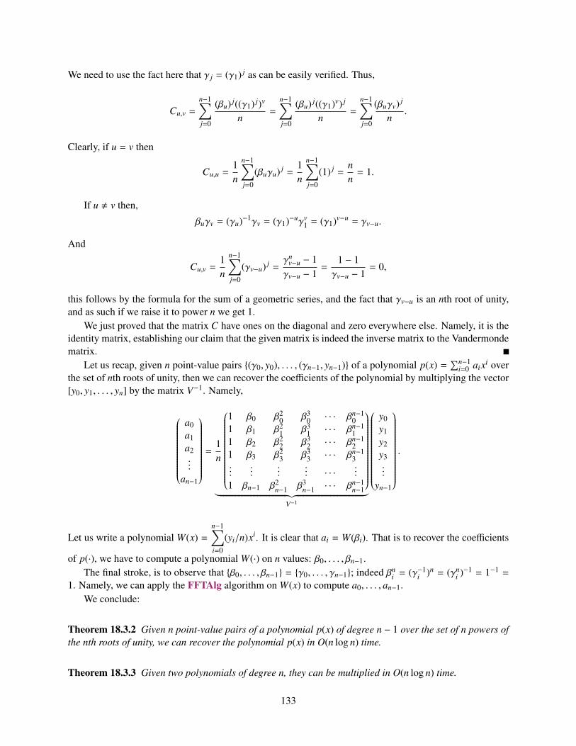
We need to use the fact here that γ j = (γ1) j as can be easily verified. Thus,

Cu,v =

n−1∑j=0

(βu) j((γ1) j)v

n=

n−1∑j=0

(βu) j((γ1)v) j

n=

n−1∑j=0

(βuγv) j

n.

Clearly, if u = v then

Cu,u =1n

n−1∑j=0

(βuγu) j =1n

n−1∑j=0

(1) j =nn= 1.

If u , v then,

βuγv = (γu)−1γv = (γ1)−uγv1 = (γ1)v−u = γv−u.

And

Cu,v =1n

n−1∑j=0

(γv−u) j =γn

v−u − 1γv−u − 1

=1 − 1γv−u − 1

= 0,

this follows by the formula for the sum of a geometric series, and the fact that γv−u is an nth root of unity,and as such if we raise it to power n we get 1.

We just proved that the matrix C have ones on the diagonal and zero everywhere else. Namely, it is theidentity matrix, establishing our claim that the given matrix is indeed the inverse matrix to the Vandermondematrix.

Let us recap, given n point-value pairs (γ0, y0), . . . , (γn−1, yn−1) of a polynomial p(x) =∑n−1

i=0 aixi overthe set of nth roots of unity, then we can recover the coefficients of the polynomial by multiplying the vector[y0, y1, . . . , yn] by the matrix V−1. Namely,

a0a1a2...

an−1

=

1n

1 β0 β20 β3

0 · · · βn−10

1 β1 β21 β3

1 · · · βn−11

1 β2 β22 β3

2 · · · βn−12

1 β3 β23 β3

3 · · · βn−13

......

...... · · ·

...

1 βn−1 β2n−1 β3

n−1 · · · βn−1n−1

︸︷︷︸V−1

y0y1y2y3...

yn−1

.

Let us write a polynomial W(x) =n−1∑i=0

(yi/n)xi. It is clear that ai = W(βi). That is to recover the coefficients

of p(·), we have to compute a polynomial W(·) on n values: β0, . . . , βn−1.The final stroke, is to observe that β0, . . . , βn−1 = γ0, . . . , γn−1; indeed βn

i = (γ−1i )n = (γn

i )−1 = 1−1 =

1. Namely, we can apply the FFTAlg algorithm on W(x) to compute a0, . . . , an−1.We conclude:

Theorem 18.3.2 Given n point-value pairs of a polynomial p(x) of degree n − 1 over the set of n powers ofthe nth roots of unity, we can recover the polynomial p(x) in O(n log n) time.

Theorem 18.3.3 Given two polynomials of degree n, they can be multiplied in O(n log n) time.

133

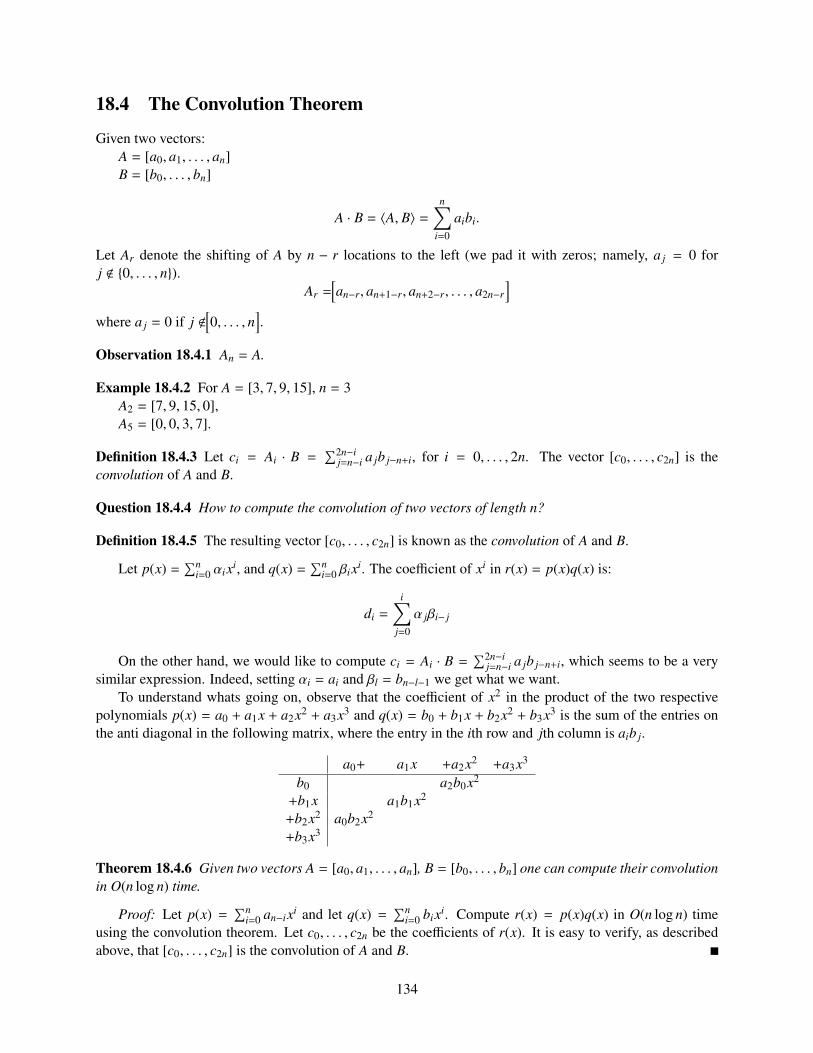
18.4 The Convolution Theorem

Given two vectors:A = [a0, a1, . . . , an]B = [b0, . . . , bn]

A · B = 〈A, B〉 =n∑

i=0

aibi.

Let Ar denote the shifting of A by n − r locations to the left (we pad it with zeros; namely, a j = 0 forj < 0, . . . , n).

Ar =[an−r, an+1−r, an+2−r, . . . , a2n−r

]where a j = 0 if j <

[0, . . . , n

].

Observation 18.4.1 An = A.

Example 18.4.2 For A = [3, 7, 9, 15], n = 3A2 = [7, 9, 15, 0],A5 = [0, 0, 3, 7].

Definition 18.4.3 Let ci = Ai · B =∑2n−i

j=n−i a jb j−n+i, for i = 0, . . . , 2n. The vector [c0, . . . , c2n] is theconvolution of A and B.

Question 18.4.4 How to compute the convolution of two vectors of length n?

Definition 18.4.5 The resulting vector [c0, . . . , c2n] is known as the convolution of A and B.

Let p(x) =∑n

i=0 αixi, and q(x) =∑n

i=0 βixi. The coefficient of xi in r(x) = p(x)q(x) is:

di =

i∑j=0

α jβi− j

On the other hand, we would like to compute ci = Ai · B =∑2n−i

j=n−i a jb j−n+i, which seems to be a verysimilar expression. Indeed, setting αi = ai and βl = bn−l−1 we get what we want.

To understand whats going on, observe that the coefficient of x2 in the product of the two respectivepolynomials p(x) = a0 + a1x + a2x2 + a3x3 and q(x) = b0 + b1x + b2x2 + b3x3 is the sum of the entries onthe anti diagonal in the following matrix, where the entry in the ith row and jth column is aib j.

a0+ a1x +a2x2 +a3x3

b0 a2b0x2

+b1x a1b1x2

+b2x2 a0b2x2

+b3x3

Theorem 18.4.6 Given two vectors A = [a0, a1, . . . , an], B = [b0, . . . , bn] one can compute their convolutionin O(n log n) time.

Proof: Let p(x) =∑n

i=0 an−ixi and let q(x) =∑n

i=0 bixi. Compute r(x) = p(x)q(x) in O(n log n) timeusing the convolution theorem. Let c0, . . . , c2n be the coefficients of r(x). It is easy to verify, as describedabove, that [c0, . . . , c2n] is the convolution of A and B.

134

Part VII

Sorting Networks

135

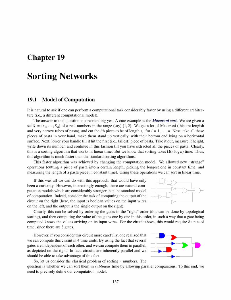
Chapter 19

Sorting Networks

19.1 Model of Computation

It is natural to ask if one can perform a computational task considerably faster by using a different architec-ture (i.e., a different computational model).

The answer to this question is a resounding yes. A cute example is the Macaroni sort. We are given aset S = s1, . . . , S n of n real numbers in the range (say) [1, 2]. We get a lot of Macaroni (this are longishand very narrow tubes of pasta), and cut the ith piece to be of length si, for i = 1, . . . , n. Next, take all thesepieces of pasta in your hand, make them stand up vertically, with their bottom end lying on a horizontalsurface. Next, lower your handle till it hit the first (i.e., tallest) piece of pasta. Take it out, measure it height,write down its number, and continue in this fashion till you have extracted all the pieces of pasta. Clearly,this is a sorting algorithm that works in linear time. But we know that sorting takes Ω(n log n) time. Thus,this algorithm is much faster than the standard sorting algorithms.

This faster algorithm was achieved by changing the computation model. We allowed new “strange”operations (cutting a piece of pasta into a certain length, picking the longest one in constant time, andmeasuring the length of a pasta piece in constant time). Using these operations we can sort in linear time.

If this was all we can do with this approach, that would have onlybeen a curiosity. However, interestingly enough, there are natural com-putation models which are considerably stronger than the standard modelof computation. Indeed, consider the task of computing the output of thecircuit on the right (here, the input is boolean values on the input wireson the left, and the output is the single output on the right).

Clearly, this can be solved by ordering the gates in the “right” order (this can be done by topologicalsorting), and then computing the value of the gates one by one in this order, in such a way that a gate beingcomputed knows the values arriving on its input wires. For the circuit above, this would require 8 units oftime, since there are 8 gates.

However, if you consider this circuit more carefully, one realized thatwe can compute this circuit in 4 time units. By using the fact that severalgates are independent of each other, and we can compute them in parallel,as depicted on the right. In fact, circuits are inherently parallel and weshould be able to take advantage of this fact.

So, let us consider the classical problem of sorting n numbers. Thequestion is whether we can sort them in sublinear time by allowing parallel comparisons. To this end, weneed to precisely define our computation model.

137

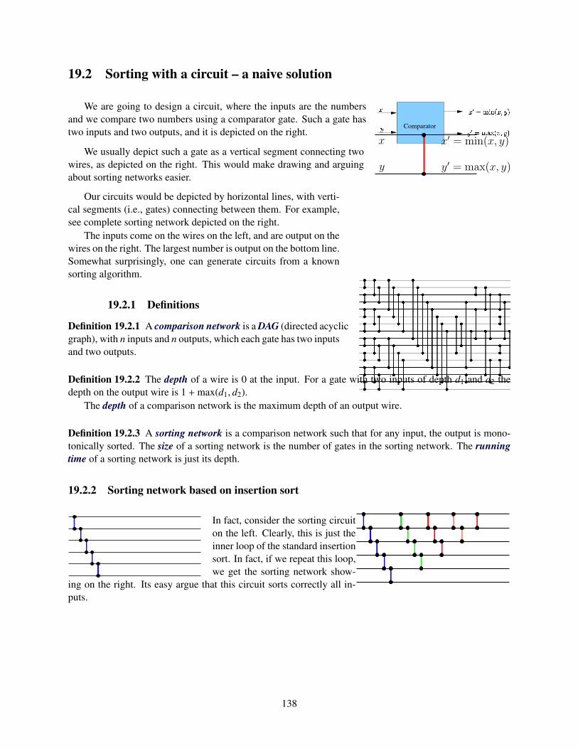
19.2 Sorting with a circuit – a naive solution

Comparator

We are going to design a circuit, where the inputs are the numbersand we compare two numbers using a comparator gate. Such a gate hastwo inputs and two outputs, and it is depicted on the right.

y

x′ = min(x, y)

y′ = max(x, y)

xWe usually depict such a gate as a vertical segment connecting two

wires, as depicted on the right. This would make drawing and arguingabout sorting networks easier.

Our circuits would be depicted by horizontal lines, with verti-cal segments (i.e., gates) connecting between them. For example,see complete sorting network depicted on the right.

The inputs come on the wires on the left, and are output on thewires on the right. The largest number is output on the bottom line.Somewhat surprisingly, one can generate circuits from a knownsorting algorithm.

19.2.1 Definitions

Definition 19.2.1 A comparison network is a DAG (directed acyclicgraph), with n inputs and n outputs, which each gate has two inputsand two outputs.

Definition 19.2.2 The depth of a wire is 0 at the input. For a gate with two inputs of depth d1 and d2 thedepth on the output wire is 1 +max(d1, d2).

The depth of a comparison network is the maximum depth of an output wire.

Definition 19.2.3 A sorting network is a comparison network such that for any input, the output is mono-tonically sorted. The size of a sorting network is the number of gates in the sorting network. The runningtime of a sorting network is just its depth.

19.2.2 Sorting network based on insertion sort

In fact, consider the sorting circuiton the left. Clearly, this is just theinner loop of the standard insertionsort. In fact, if we repeat this loop,we get the sorting network show-

ing on the right. Its easy argue that this circuit sorts correctly all in-puts.

138

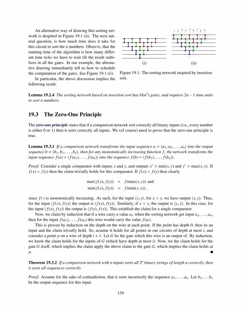
1 2 3 4 5 6 7 8 9

(i) (ii)

Figure 19.1: The sorting network inspired by insertionsort.

An alternative way of drawing this sorting net-work is despited in Figure 19.1 (ii). The next nat-ural question, is how much time does it take forthis circuit to sort the n numbers. Observe, that therunning time of the algorithm is how many differ-ent time ticks we have to wait till the result stabi-lizes in all the gates. In our example, the alterna-tive drawing immediately tell us how to schedulethe computation of the gates. See Figure 19.1 (ii).

In particular, the above discussion implies thefollowing result.

Lemma 19.2.4 The sorting network based on insertion sort has O(n2) gates, and requires 2n− 1 time unitsto sort n numbers.

19.3 The Zero-One Principle

The zero-one principle states that if a comparison network sort correctly all binary inputs (i.e., every numberis either 0 or 1) then it sorts correctly all inputs. We (of course) need to prove that the zero-one principle istrue.

Lemma 19.3.1 If a comparison network transforms the input sequence a = 〈a1, a2, . . . , an〉 into the outputsequence b = 〈b1, b2, . . . , bn〉, then for any monotonically increasing function f , the network transforms theinput sequence f (a) = 〈 f (a1), . . . , f (an)〉 into the sequence f (b) = 〈 f (b1), . . . , f (bn)〉.

Proof: Consider a single comparator with inputs x and y, and outputs x′ = min(x, y) and y′ = max(x, y). Iff (x) = f (y) then the claim trivially holds for this comparator. If f (x) < f (y) then clearly

max( f (x), f (y)) = f (max(x, y)) and

min( f (x), f (y)) = f (min(x, y)) ,

since f (·) is monotonically increasing. As such, for the input 〈x, y〉, for x < y, we have output 〈x, y〉. Thus,for the input 〈 f (x), f (y)〉 the output is 〈 f (x), f (y)〉. Similarly, if x > y, the output is 〈y, x〉. In this case, forthe input 〈 f (x), f (y)〉 the output is 〈 f (y), f (x)〉. This establish the claim for a single comparator.

Now, we claim by induction that if a wire carry a value ai, when the sorting network get input a1, . . . , an,then for the input f (a1), . . . , f (an) this wire would carry the value f (ai).

This is proven by induction on the depth on the wire at each point. If the point has depth 0, then its aninput and the claim trivially hold. So, assume it holds for all points in our circuits of depth at most i, andconsider a point p on a wire of depth i + 1. Let G be the gate which this wire is an output of. By induction,we know the claim holds for the inputs of G (which have depth at most i). Now, we the claim holds for thegate G itself, which implies the claim apply the above claim to the gate G, which implies the claim holds atp.

Theorem 19.3.2 If a comparison network with n inputs sorts all 2n binary strings of length n correctly, thenit sorts all sequences correctly.

Proof: Assume for the sake of contradiction, that it sorts incorrectly the sequence a1, . . . , an. Let b1, . . . bn

be the output sequence for this input.

139

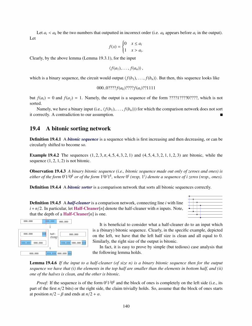
Let ai < ak be the two numbers that outputted in incorrect order (i.e. ak appears before ai in the output).Let

f (x) =

0 x ≤ ai

1 x > ai.

Clearly, by the above lemma (Lemma 19.3.1), for the input

〈 f (a1), . . . , f (an)〉 ,

which is a binary sequence, the circuit would output 〈 f (b1), . . . , f (bn)〉. But then, this sequence looks like

000..0???? f (ak)???? f (ai)??1111

but f (ai) = 0 and f (a j) = 1. Namely, the output is a sequence of the form ????1????0????, which is notsorted.

Namely, we have a binary input (i.e., 〈 f (b1), . . . , f (bn)〉) for which the comparison network does not sortit correctly. A contradiction to our assumption.

19.4 A bitonic sorting network

Definition 19.4.1 A bitonic sequence is a sequence which is first increasing and then decreasing, or can becircularly shifted to become so.

Example 19.4.2 The sequences (1, 2, 3, π, 4, 5, 4, 3, 2, 1) and (4, 5, 4, 3, 2, 1, 1, 2, 3) are bitonic, while thesequence (1, 2, 1, 2) is not bitonic.

Observation 19.4.3 A binary bitonic sequence (i.e., bitonic sequence made out only of zeroes and ones) iseither of the form 0i1 j0k or of the form 1i0 j1k, where 0i (resp, 1i) denote a sequence of i zeros (resp., ones).

Definition 19.4.4 A bitonic sorter is a comparison network that sorts all bitonic sequences correctly.

Definition 19.4.5 A half-cleaner is a comparison network, connecting line i with linei+ n/2. In particular, let Half-Cleaner[n] denote the half-cleaner with n inputs. Note,that the depth of a Half-Cleaner[n] is one.

111..111 000..000000..000

000..000111..111 111..111 111

000..000

000..000

111..111 111000..000

000..000 111

000..000

half−

cleaner

It is beneficial to consider what a half-cleaner do to an input whichis a (binary) bitonic sequence. Clearly, in the specific example, depictedon the left, we have that the left half size is clean and all equal to 0.Similarly, the right size of the output is bitonic.

In fact, it is easy to prove by simple (but tedious) case analysis thatthe following lemma holds.

Lemma 19.4.6 If the input to a half-cleaner (of size n) is a binary bitonic sequence then for the outputsequence we have that (i) the elements in the top half are smaller than the elements in bottom half, and (ii)one of the halves is clean, and the other is bitonic.

Proof: If the sequence is of the form 0i1 j0k and the block of ones is completely on the left side (i.e., itspart of the first n/2 bits) or the right side, the claim trivially holds. So, assume that the block of ones startsat position n/2 − β and ends at n/2 + α.

140

"!#%$&'(*)

+ ,!#-$

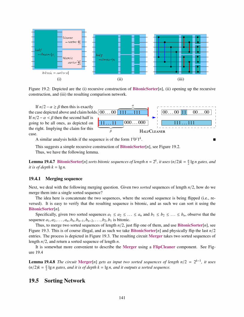
(i) (ii) (iii)

Figure 19.2: Depicted are the (i) recursive construction of BitonicSorter[n], (ii) opening up the recursiveconstruction, and (iii) the resulting comparison network.

00 . . . 00 111 . . . 111

000 . . . 00011 . . . 11

HC

00 . . . 00 00 . . . 0011

111 . . . 111

α︷︸︸︷︸︷︷︸

β

If n/2−α ≥ β then this is exactlythe case depicted above and claim holds.If n/2− α < β then the second half isgoing to be all ones, as depicted onthe right. Implying the claim for thiscase.

A similar analysis holds if the sequence is of the form 1i0 j1k.

This suggests a simple recursive construction of BitonicSorter[n], see Figure 19.2.Thus, we have the following lemma.

Lemma 19.4.7 BitonicSorter[n] sorts bitonic sequences of length n = 2k, it uses (n/2)k = n2 lg n gates, and

it is of depth k = lg n.

19.4.1 Merging sequence

Next, we deal with the following merging question. Given two sorted sequences of length n/2, how do wemerge them into a single sorted sequence?

The idea here is concatenate the two sequences, where the second sequence is being flipped (i.e., re-versed). It is easy to verify that the resulting sequence is bitonic, and as such we can sort it using theBitonicSorter[n].

Specifically, given two sorted sequences a1 ≤ a2 ≤ . . . ≤ an and b1 ≤ b2 ≤ . . . ≤ bn, observe that thesequence a1, a2, . . . , an, bn, bn−1, bn−2, . . . , b2, b1 is bitonic.

Thus, to merge two sorted sequences of length n/2, just flip one of them, and use BitonicSorter[n], seeFigure 19.3. This is of course illegal, and as such we take BitonicSorter[n] and physically flip the last n/2entries. The process is depicted in Figure 19.3. The resulting circuit Merger takes two sorted sequences oflength n/2, and return a sorted sequence of length n.

It is somewhat more convenient to describe the Merger using a FlipCleaner component. See Fig-ure 19.4

Lemma 19.4.8 The circuit Merger[n] gets as input two sorted sequences of length n/2 = 2k−1, it uses(n/2)k = n

2 lg n gates, and it is of depth k = lg n, and it outputs a sorted sequence.

19.5 Sorting Network

141

(i) (ii) (iii) (iv)

Figure 19.3: (i) Merger via flipping the lines of bitonic sorter. (ii) A BitonicSorter. (ii) The Merger afterwe “physically” flip the lines, and (iv) An equivalent drawing of the resulting Merger.

!#"%$ &('

! "%$ &('

(i) (ii)

Figure 19.4: (i) FlipCleaner[n], and (ii) Merger[n] described using FlipCleaner.

We are now in the stage, where we can build a sorting network. Tothis end, we just implement merge sort using the Merger[n] component.The resulting component Sorter[n] is despited on the right using a recur-sive construction.

Lemma 19.5.1 The circuit Sorter[n] is a sorting network (i.e., it sortsany n numbers) using G(n) = O(n log2 n) gates. It has depth O(log2 n).Namely, Sorter[n] sorts n numbers in O(log2 n) time.

Proof: The number of gates is

G(n) = 2G(n/2) +Gates(Merger[n]).

Which is G(n) = 2G(n/2) + O(n log n) = O(n log2 n).As for the depth, we have that D(n) = D(n/2) + Depth(Merger[n]) = D(n/2) + O(log(n)), and thus

D(n) = O(log2 n), as claimed.

19.6 Faster sorting networks

Figure 19.5: Sorter[8].

One can build a sorting network of logarithmic depth (see [AKS83]).The construction however is very complicated. A simpler parallel algo-rithm would be discussed sometime in the next lectures. BTW, the AKSconstruction [AKS83] mentioned above, is better than bitonic sort for nlarger than 28046.

142

Part VIII

Linear Programming

143

Chapter 20

Linear Programming

20.1 Introduction and Motivation

In the VCR/guns/nuclear-bombs/napkins/star-wars/professors/butter/mice problem, the benevolent dictator,Biga Piguinus, of Penguina (a country in south Antarctica having 24 million penguins under its control) hasto decide how to allocate her empire resources to the maximal benefit of her penguins. In particular, she hasto decide how to allocate the money for the next year budget. For example, buying a nuclear bomb has atremendous positive effect on security (the ability to destruct yourself completely together with your enemyinduces a peaceful serenity feeling in most people). Guns, on the other hand, have a weaker effect. Penguina(the state) has to supply a certain level of security. Thus, the allocation should be such that:

xgun + 1000 ∗ xnuclear−bomb ≥ 1000,

where xguns is the number of guns constructed, and xnuclear−bomb is the number of nuclear-bombs constructed.On the other hand,

100 ∗ xgun + 1000000 ∗ xnuclear−bomb ≤ xsecurity

where xsecurity is the total Penguina is willing to spend on security, and 100 is the price of producing a singlegun, and 1, 000, 000 is the price of manufacturing one nuclear bomb. There are a lot of other constrains ofthis type, and Biga Piguinus would like to solve them, while minimizing the total money allocated for suchspending (the less spent on budget, the larger the tax cut).

a11x1 + . . . + a1nxn ≤ b1a21x1 + . . . + a2nxn ≤ b2. . .

am1x1 + . . . + amnxn ≤ bm

max c1x1 + . . . + cnxn.

More formally, we have a (potentially large) number of variables: x1, . . . ,

xn and a (potentially large) system of linear inequalities. We will refer tosuch an inequality as a constraint. We would like to decide if there is anassignment of values to x1, . . . , xn where all these inequalities are satisfied.Since there might be infinite number of such solutions, we want the solutionthat maximizes some linear quantity. See the instance on the right.

The linear target function we are trying to maximize is known as the objective function of the linearprogram. Such a problem is an instance of linear programming. We refer to linear programming as LP.

20.1.1 History

Linear programming can be traced back to the early 19th century. It started in earnest in 1939 when L. V.Kantorovich noticed the importance of certain type of Linear Programming problems. Unfortunately, forseveral years, Kantorovich work was unknown in the west and unnoticed in the east.

Dantzig, in 1947, invented the simplex method for solving LP problems for the US Air force planningproblems.

145

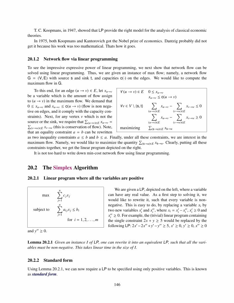
T. C. Koopmans, in 1947, showed that LP provide the right model for the analysis of classical economictheories.

In 1975, both Koopmans and Kantorovich got the Nobel prize of economics. Dantzig probably did notget it because his work was too mathematical. Thats how it goes.

20.1.2 Network flow via linear programming

To see the impressive expressive power of linear programming, we next show that network flow can besolved using linear programming. Thus, we are given an instance of max flow; namely, a network flowG = (V,E) with source s and sink t, and capacities c(·) on the edges. We would like to compute themaximum flow in G.

∀ (u→ v) ∈ E 0 ≤ xu→v

xu→v ≤ c(u→ v)

∀v ∈ V \ s, t∑

(u→v)∈E

xu→v −∑

(v→w)∈E

xv→w ≤ 0∑(u→v)∈E

xu→v −∑

(v→w)∈E

xv→w ≥ 0

maximizing∑

(s→u)∈E xs→u

To this end, for an edge (u→ v) ∈ E, let xu→v

be a variable which is the amount of flow assignto (u→ v) in the maximum flow. We demand that0 ≤ xu→v and xu→v ≤ c(u→ v) (flow is non nega-tive on edges, and it comply with the capacity con-straints). Next, for any vertex v which is not thesource or the sink, we require that

∑(u→v)∈E xu→v =∑

(v→w)∈E xv→w (this is conservation of flow). Note,that an equality constraint a = b can be rewrittenas two inequality constraints a ≤ b and b ≤ a. Finally, under all these constraints, we are interest in themaximum flow. Namely, we would like to maximize the quantity

∑(s→u)∈E xs→u. Clearly, putting all these

constraints together, we get the linear program depicted on the right.It is not too hard to write down min-cost network flow using linear programming.

20.2 The Simplex Algorithm

20.2.1 Linear program where all the variables are positive

maxn∑

j=1

c jx j

subject ton∑

j=1

ai jx j ≤ bi

for i = 1, 2, . . . ,m

We are given a LP, depicted on the left, where a variablecan have any real value. As a first step to solving it, wewould like to rewrite it, such that every variable is non-negative. This is easy to do, by replacing a variable xi bytwo new variables x′i and x′′i , where xi = x′i − x′′i , x′i ≥ 0 andx′′i ≥ 0. For example, the (trivial) linear program containingthe single constraint 2x + y ≥ 5 would be replaced by thefollowing LP: 2x′−2x′′+y′−y′′ ≥ 5, x′ ≥ 0, y′ ≥ 0, x′′ ≥ 0

and y′′ ≥ 0.

Lemma 20.2.1 Given an instance I of LP, one can rewrite it into an equivalent LP, such that all the vari-ables must be non-negative. This takes linear time in the size of I.

20.2.2 Standard form

Using Lemma 20.2.1, we can now require a LP to be specified using only positive variables. This is knownas standard form.

146

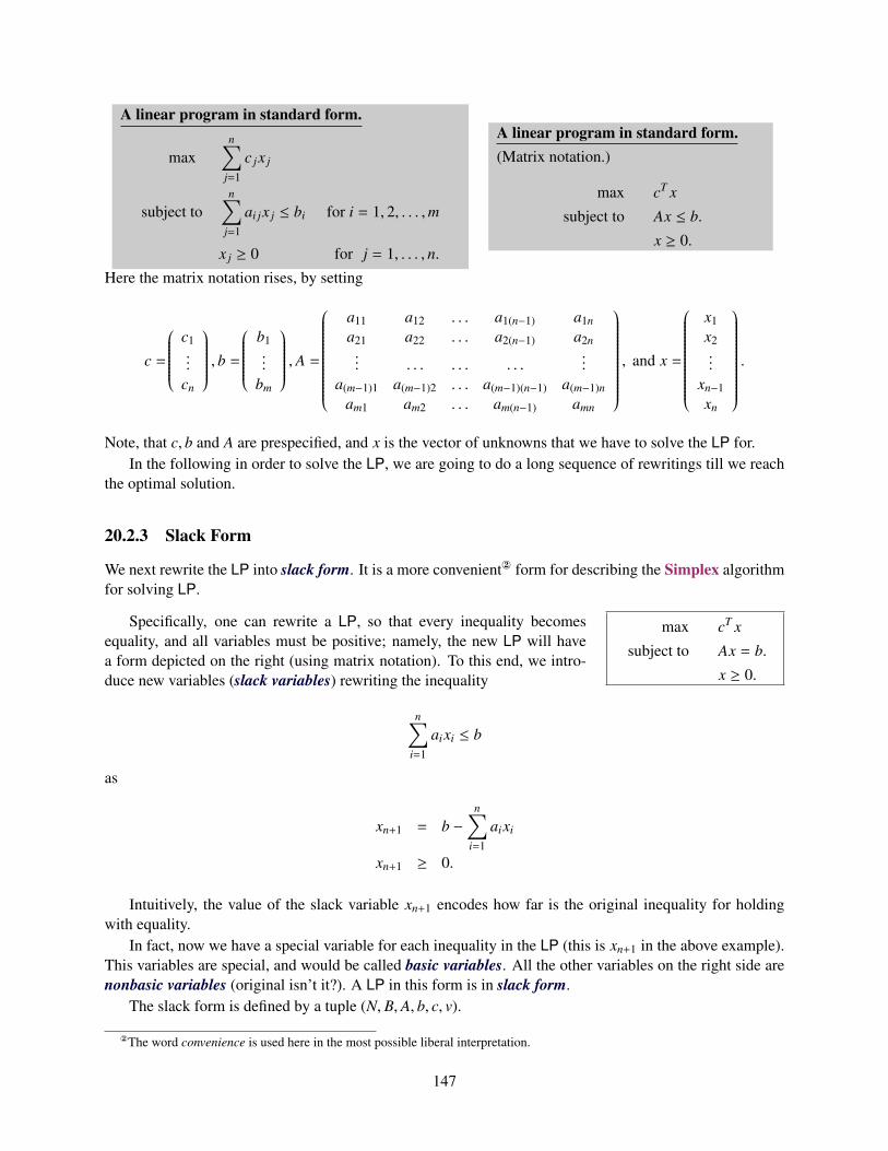
A linear program in standard form.

maxn∑

j=1

c jx j

subject ton∑

j=1

ai jx j ≤ bi for i = 1, 2, . . . ,m

x j ≥ 0 for j = 1, . . . , n.

A linear program in standard form.(Matrix notation.)

max cT x

subject to Ax ≤ b.

x ≥ 0.

Here the matrix notation rises, by setting

c =

c1...

cn

, b =

b1...

bm

, A =

a11 a12 . . . a1(n−1) a1n

a21 a22 . . . a2(n−1) a2n... . . . . . . . . .

...

a(m−1)1 a(m−1)2 . . . a(m−1)(n−1) a(m−1)nam1 am2 . . . am(n−1) amn

, and x =

x1x2...

xn−1xn

.

Note, that c, b and A are prespecified, and x is the vector of unknowns that we have to solve the LP for.In the following in order to solve the LP, we are going to do a long sequence of rewritings till we reach

the optimal solution.

20.2.3 Slack Form

We next rewrite the LP into slack form. It is a more convenient form for describing the Simplex algorithmfor solving LP.

max cT x

subject to Ax = b.

x ≥ 0.

Specifically, one can rewrite a LP, so that every inequality becomesequality, and all variables must be positive; namely, the new LP will havea form depicted on the right (using matrix notation). To this end, we intro-duce new variables (slack variables) rewriting the inequality

n∑i=1

aixi ≤ b

as

xn+1 = b −n∑

i=1

aixi

xn+1 ≥ 0.

Intuitively, the value of the slack variable xn+1 encodes how far is the original inequality for holdingwith equality.

In fact, now we have a special variable for each inequality in the LP (this is xn+1 in the above example).This variables are special, and would be called basic variables. All the other variables on the right side arenonbasic variables (original isn’t it?). A LP in this form is in slack form.

The slack form is defined by a tuple (N, B, A, b, c, v).

The word convenience is used here in the most possible liberal interpretation.

147

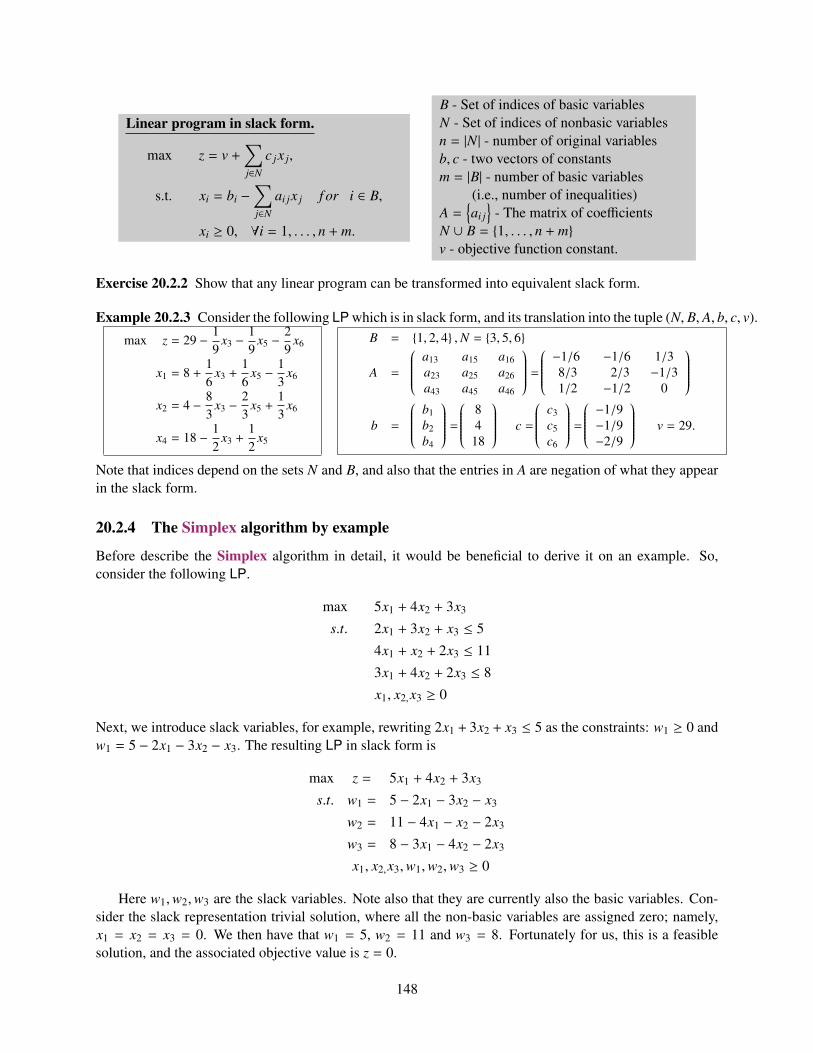
Linear program in slack form.

max z = v +∑j∈N

c jx j,

s.t. xi = bi −∑j∈N

ai jx j f or i ∈ B,

xi ≥ 0, ∀i = 1, . . . , n + m.

B - Set of indices of basic variablesN - Set of indices of nonbasic variablesn = |N | - number of original variablesb, c - two vectors of constantsm = |B| - number of basic variables

(i.e., number of inequalities)A =

ai j

- The matrix of coefficients

N ∪ B = 1, . . . , n + mv - objective function constant.

Exercise 20.2.2 Show that any linear program can be transformed into equivalent slack form.

Example 20.2.3 Consider the following LP which is in slack form, and its translation into the tuple (N, B, A, b, c, v).

max z = 29 −19

x3 −19

x5 −29

x6

x1 = 8 +16

x3 +16

x5 −13

x6

x2 = 4 −83

x3 −23

x5 +13

x6

x4 = 18 −12

x3 +12

x5

B = 1, 2, 4 ,N = 3, 5, 6

A =

a13 a15 a16a23 a25 a26a43 a45 a46

= −1/6 −1/6 1/3

8/3 2/3 −1/31/2 −1/2 0

b =

b1b2b4

= 8

418

c =

c3c5c6

= −1/9−1/9−2/9

v = 29.

Note that indices depend on the sets N and B, and also that the entries in A are negation of what they appearin the slack form.

20.2.4 The Simplex algorithm by example

Before describe the Simplex algorithm in detail, it would be beneficial to derive it on an example. So,consider the following LP.

max 5x1 + 4x2 + 3x3

s.t. 2x1 + 3x2 + x3 ≤ 5

4x1 + x2 + 2x3 ≤ 11

3x1 + 4x2 + 2x3 ≤ 8

x1, x2,x3 ≥ 0

Next, we introduce slack variables, for example, rewriting 2x1 + 3x2 + x3 ≤ 5 as the constraints: w1 ≥ 0 andw1 = 5 − 2x1 − 3x2 − x3. The resulting LP in slack form is

max z = 5x1 + 4x2 + 3x3

s.t. w1 = 5 − 2x1 − 3x2 − x3

w2 = 11 − 4x1 − x2 − 2x3

w3 = 8 − 3x1 − 4x2 − 2x3

x1, x2,x3,w1,w2,w3 ≥ 0

Here w1,w2,w3 are the slack variables. Note also that they are currently also the basic variables. Con-sider the slack representation trivial solution, where all the non-basic variables are assigned zero; namely,x1 = x2 = x3 = 0. We then have that w1 = 5, w2 = 11 and w3 = 8. Fortunately for us, this is a feasiblesolution, and the associated objective value is z = 0.

148

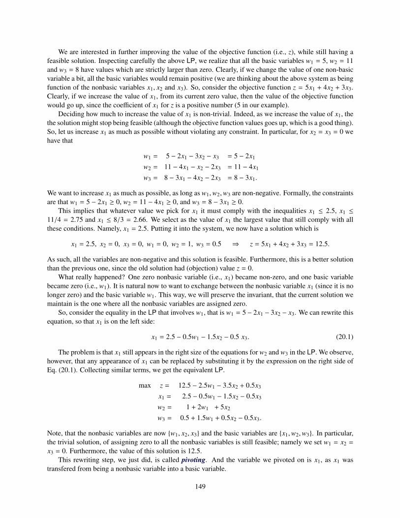
We are interested in further improving the value of the objective function (i.e., z), while still having afeasible solution. Inspecting carefully the above LP, we realize that all the basic variables w1 = 5, w2 = 11and w3 = 8 have values which are strictly larger than zero. Clearly, if we change the value of one non-basicvariable a bit, all the basic variables would remain positive (we are thinking about the above system as beingfunction of the nonbasic variables x1, x2 and x3). So, consider the objective function z = 5x1 + 4x2 + 3x3.Clearly, if we increase the value of x1, from its current zero value, then the value of the objective functionwould go up, since the coefficient of x1 for z is a positive number (5 in our example).

Deciding how much to increase the value of x1 is non-trivial. Indeed, as we increase the value of x1, thethe solution might stop being feasible (although the objective function values goes up, which is a good thing).So, let us increase x1 as much as possible without violating any constraint. In particular, for x2 = x3 = 0 wehave that

w1 = 5 − 2x1 − 3x2 − x3 = 5 − 2x1

w2 = 11 − 4x1 − x2 − 2x3 = 11 − 4x1

w3 = 8 − 3x1 − 4x2 − 2x3 = 8 − 3x1.

We want to increase x1 as much as possible, as long as w1,w2,w3 are non-negative. Formally, the constraintsare that w1 = 5 − 2x1 ≥ 0, w2 = 11 − 4x1 ≥ 0, and w3 = 8 − 3x1 ≥ 0.

This implies that whatever value we pick for x1 it must comply with the inequalities x1 ≤ 2.5, x1 ≤

11/4 = 2.75 and x1 ≤ 8/3 = 2.66. We select as the value of x1 the largest value that still comply with allthese conditions. Namely, x1 = 2.5. Putting it into the system, we now have a solution which is

x1 = 2.5, x2 = 0, x3 = 0, w1 = 0, w2 = 1, w3 = 0.5 ⇒ z = 5x1 + 4x2 + 3x3 = 12.5.

As such, all the variables are non-negative and this solution is feasible. Furthermore, this is a better solutionthan the previous one, since the old solution had (objection) value z = 0.

What really happened? One zero nonbasic variable (i.e., x1) became non-zero, and one basic variablebecame zero (i.e., w1). It is natural now to want to exchange between the nonbasic variable x1 (since it is nolonger zero) and the basic variable w1. This way, we will preserve the invariant, that the current solution wemaintain is the one where all the nonbasic variables are assigned zero.

So, consider the equality in the LP that involves w1, that is w1 = 5 − 2x1 − 3x2 − x3. We can rewrite thisequation, so that x1 is on the left side:

x1 = 2.5 − 0.5w1 − 1.5x2 − 0.5 x3. (20.1)

The problem is that x1 still appears in the right size of the equations for w2 and w3 in the LP. We observe,however, that any appearance of x1 can be replaced by substituting it by the expression on the right side ofEq. (20.1). Collecting similar terms, we get the equivalent LP.

max z = 12.5 − 2.5w1 − 3.5x2 + 0.5x3

x1 = 2.5 − 0.5w1 − 1.5x2 − 0.5x3

w2 = 1 + 2w1 + 5x2

w3 = 0.5 + 1.5w1 + 0.5x2 − 0.5x3.

Note, that the nonbasic variables are now w1, x2, x3 and the basic variables are x1,w2,w3. In particular,the trivial solution, of assigning zero to all the nonbasic variables is still feasible; namely we set w1 = x2 =

x3 = 0. Furthermore, the value of this solution is 12.5.This rewriting step, we just did, is called pivoting. And the variable we pivoted on is x1, as x1 was

transfered from being a nonbasic variable into a basic variable.

149

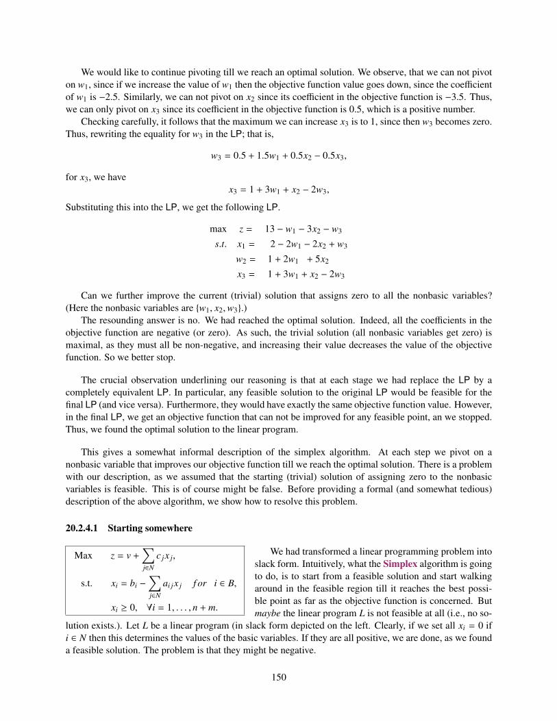
We would like to continue pivoting till we reach an optimal solution. We observe, that we can not pivoton w1, since if we increase the value of w1 then the objective function value goes down, since the coefficientof w1 is −2.5. Similarly, we can not pivot on x2 since its coefficient in the objective function is −3.5. Thus,we can only pivot on x3 since its coefficient in the objective function is 0.5, which is a positive number.

Checking carefully, it follows that the maximum we can increase x3 is to 1, since then w3 becomes zero.Thus, rewriting the equality for w3 in the LP; that is,

w3 = 0.5 + 1.5w1 + 0.5x2 − 0.5x3,

for x3, we havex3 = 1 + 3w1 + x2 − 2w3,

Substituting this into the LP, we get the following LP.

max z = 13 − w1 − 3x2 − w3

s.t. x1 = 2 − 2w1 − 2x2 + w3

w2 = 1 + 2w1 + 5x2

x3 = 1 + 3w1 + x2 − 2w3

Can we further improve the current (trivial) solution that assigns zero to all the nonbasic variables?(Here the nonbasic variables are w1, x2,w3.)

The resounding answer is no. We had reached the optimal solution. Indeed, all the coefficients in theobjective function are negative (or zero). As such, the trivial solution (all nonbasic variables get zero) ismaximal, as they must all be non-negative, and increasing their value decreases the value of the objectivefunction. So we better stop.

The crucial observation underlining our reasoning is that at each stage we had replace the LP by acompletely equivalent LP. In particular, any feasible solution to the original LP would be feasible for thefinal LP (and vice versa). Furthermore, they would have exactly the same objective function value. However,in the final LP, we get an objective function that can not be improved for any feasible point, an we stopped.Thus, we found the optimal solution to the linear program.

This gives a somewhat informal description of the simplex algorithm. At each step we pivot on anonbasic variable that improves our objective function till we reach the optimal solution. There is a problemwith our description, as we assumed that the starting (trivial) solution of assigning zero to the nonbasicvariables is feasible. This is of course might be false. Before providing a formal (and somewhat tedious)description of the above algorithm, we show how to resolve this problem.

20.2.4.1 Starting somewhere

Max z = v +∑j∈N

c jx j,

s.t. xi = bi −∑j∈N


xi ≥ 0, ∀i = 1, . . . , n + m.

We had transformed a linear programming problem intoslack form. Intuitively, what the Simplex algorithm is goingto do, is to start from a feasible solution and start walkingaround in the feasible region till it reaches the best possi-ble point as far as the objective function is concerned. Butmaybe the linear program L is not feasible at all (i.e., no so-

lution exists.). Let L be a linear program (in slack form depicted on the left. Clearly, if we set all xi = 0 ifi ∈ N then this determines the values of the basic variables. If they are all positive, we are done, as we founda feasible solution. The problem is that they might be negative.

150

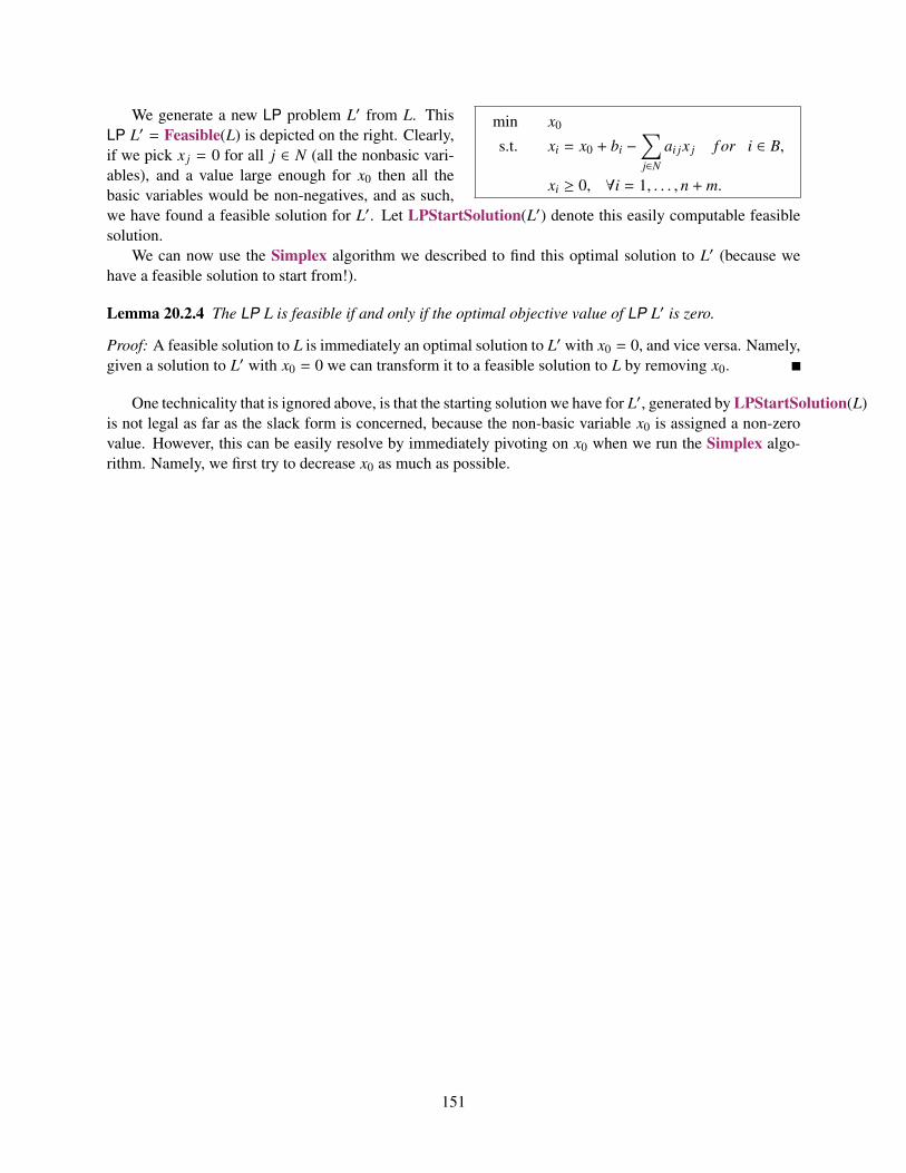
min x0

s.t. xi = x0 + bi −∑j∈N


xi ≥ 0, ∀i = 1, . . . , n + m.

We generate a new LP problem L′ from L. ThisLP L′ = Feasible(L) is depicted on the right. Clearly,if we pick x j = 0 for all j ∈ N (all the nonbasic vari-ables), and a value large enough for x0 then all thebasic variables would be non-negatives, and as such,we have found a feasible solution for L′. Let LPStartSolution(L′) denote this easily computable feasiblesolution.

We can now use the Simplex algorithm we described to find this optimal solution to L′ (because wehave a feasible solution to start from!).

Lemma 20.2.4 The LP L is feasible if and only if the optimal objective value of LP L′ is zero.

Proof: A feasible solution to L is immediately an optimal solution to L′ with x0 = 0, and vice versa. Namely,given a solution to L′ with x0 = 0 we can transform it to a feasible solution to L by removing x0.

One technicality that is ignored above, is that the starting solution we have for L′, generated by LPStartSolution(L)is not legal as far as the slack form is concerned, because the non-basic variable x0 is assigned a non-zerovalue. However, this can be easily resolve by immediately pivoting on x0 when we run the Simplex algo-rithm. Namely, we first try to decrease x0 as much as possible.

151

152

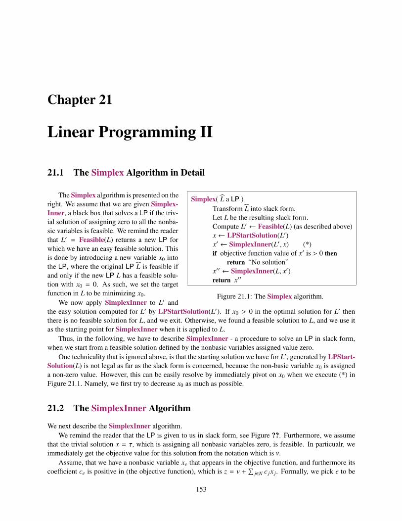
Chapter 21

Linear Programming II

21.1 The Simplex Algorithm in Detail

Simplex( L a LP )Transform L into slack form.Let L be the resulting slack form.Compute L′ ← Feasible(L) (as described above)x← LPStartSolution(L′)x′ ← SimplexInner(L′, x) (*)if objective function value of x′ is > 0 then

return “No solution”x′′ ← SimplexInner(L, x′)return x′′

Figure 21.1: The Simplex algorithm.

The Simplex algorithm is presented on theright. We assume that we are given Simplex-Inner, a black box that solves a LP if the triv-ial solution of assigning zero to all the nonba-sic variables is feasible. We remind the readerthat L′ = Feasible(L) returns a new LP forwhich we have an easy feasible solution. Thisis done by introducing a new variable x0 intothe LP, where the original LP L is feasible ifand only if the new LP L has a feasible solu-tion with x0 = 0. As such, we set the targetfunction in L to be minimizing x0.

We now apply SimplexInner to L′ andthe easy solution computed for L′ by LPStartSolution(L′). If x0 > 0 in the optimal solution for L′ thenthere is no feasible solution for L, and we exit. Otherwise, we found a feasible solution to L, and we use itas the starting point for SimplexInner when it is applied to L.

Thus, in the following, we have to describe SimplexInner - a procedure to solve an LP in slack form,when we start from a feasible solution defined by the nonbasic variables assigned value zero.

One technicality that is ignored above, is that the starting solution we have for L′, generated by LPStart-Solution(L) is not legal as far as the slack form is concerned, because the non-basic variable x0 is assigneda non-zero value. However, this can be easily resolve by immediately pivot on x0 when we execute (*) inFigure 21.1. Namely, we first try to decrease x0 as much as possible.

21.2 The SimplexInner Algorithm

We next describe the SimplexInner algorithm.We remind the reader that the LP is given to us in slack form, see Figure ??. Furthermore, we assume

that the trivial solution x = τ, which is assigning all nonbasic variables zero, is feasible. In particualr, weimmediately get the objective value for this solution from the notation which is v.

Assume, that we have a nonbasic variable xe that appears in the objective function, and furthermore itscoefficient ce is positive in (the objective function), which is z = v +

∑j∈N c jx j. Formally, we pick e to be

153

one of the indices of j∣∣∣ c j > 0, j ∈ N

.

The variable xe is the entering variable variable (since it is going to join the set of basic variables).Clearly, if we increase the value of xe (from the current value of 0 in τ) then one of the basic variables is

going to vanish (i.e., become zero). Let xl be this basic variable. We increase the value of xe (the enteringvariable) till xl (the leaving variable) becomes zero.

Setting all nonbasic variables to zero, and letting xe grow, implies that xi = bi − aiexe, for all i ∈ B.All those variables must be non-negative, and thus we require that ∀i ∈ B it holds xi = bi − aiexe ≥ 0.

Namely, xe ≤ (bi/aie) or alternatively,1xe≥

aie

bi. Namely,

1xe≥ max

i∈B

aie

biand, the largest value of xe which is

still feasible is

U =(maxi∈B

aie

bi

)−1

.

We pick l (the index of the leaving variable) from the set all basic variables that vanish to zero when xe = U.Namely, l is from the set

j

∣∣∣∣∣∣ a je

b j= U where j ∈ B

.

Now, we know xe and xl. We rewrite the equation for xl in the LP so that it has xe on the left size.Formally, we do

xl = bl −∑j∈N

al jx j ⇒ xe =bl

ale−

∑j∈N∪l

al j

alex j, where all = 1.

We need to remove all the appearances on the right side of the LP of xe. This can be done by substitutingxe into the other equalities, using the above equality. Alternatively, we do beforehand Gaussian elimination,to remove any appearance of xe on the right side of the equalities in the LP (and also from the objectivefunction) replaced by appearances of xl on the left side, which we then transfer to the right side.

In the end of this process, we have a new equivalent LP where the basic variables are B′ = (B \ l)∪ eand the non-basic variables are N′ = (N \ e) ∪ l.

In end of this pivoting stage the LP objective function value had increased, and as such, we madeprogress. Note, that the linear system is completely defined by which variables are basic, and which arenon-basic. Furthermore, pivoting never returns to a combination (of basic/non-basic variable) that wasalready visited. Indeed, we improve the value of the objective function in each pivoting stage. Thus, we cando at most (

n + mn

)≤

(n + mn· e

)n

pivoting steps. And this is close to tight in the worst case (there are examples where 2n pivoting steps areneeded.

Each pivoting step takes polynomial time in n and m. Thus, the overall running time of Simplex isexponential in the worst case. However, in practice, Simplex is extremely fast.

21.2.1 Degeneracies

If you inspect carefully the Simplex algorithm, you would notice that it might get stuck if one of the bis iszero. This corresponds to a case where > m hyperplanes passes through the same point. This might causethe effect that you might not be able to make any progress at all in pivoting.

154

There are several solutions, the simplest one is to add tiny random noise to each coefficient. You caneven do this symbolically. Intuitively, the degeneracy, being a local phenomena on the polytope disappearswith high probability.

The larger danger, is that you would get into cycling; namely, a sequence of pivoting operations that donot improve the objective function, and the bases you get are cyclic (i.e., infinite loop).

There is a simple scheme based on using the symbolic perturbation, that avoids cycling, by carefullychoosing what is the leaving variable. We omit all further details here.

There is an alternative approach, called Bland’s rule, which always choose the lowest index variable forentering and leaving out of the possible candidates. We will not prove the correctness of this approach here.

21.2.2 Correctness of linear programming

Theorem 21.2.1 (Fundamental theorem of Linear Programming.) For an arbitrary linear program, thefollowing statements are true:

1. If there is no optimal solution, the problem is either infeasible or unbounded.

2. If a feasible solution exists, then a basic feasible solution exists.

3. If an optimal solution exists, then a basic optimal solution exists.

Proof: Proof is constructive by running the simplex algorithm.

21.2.3 On the ellipsoid method and interior point methods

The Simplex algorithm has exponential running time in the worst case.The ellipsoid method is weakly polynomial (namely, it is polynomial in the number of bits of the input).

Khachian in 1979 came up with it. It turned out to be completely useless in practice.In 1984, Karmakar came up with a different method, called the interior-point method which is also

weakly polynomial. However, it turned out to be quite useful in practice, resulting in an arm race betweenthe interior-point method and the simplex method.

The question of whether there is a strongly polynomial time algorithm for linear programming, is one ofthe major open questions in computer science.

21.3 Duality and Linear Programming

Every linear program L has a dual linear program L′. Solving the dual problem is essentially equivalent tosolving the primal linear program (i.e., the original) LP.

21.3.1 Duality by Example

max z = 4x1 + x2 + 3x3

s.t. x1 + 4x2 ≤ 1

3x1 − x2 + x3 ≤ 3

x1, x2, x3 ≥ 0Figure 21.2: The linear programL.

Consider the linear program L depicted on the right (Figure 21.2).Note, that any feasible solution, gives us a lower bound on the maximalvalue of the target function, denoted by η. In particular, the solutionx1 = 1, x2 = x3 = 0 is feasible, and implies z = 4 and thus η ≥ 4.

Similarly, x1 = x2 = 0, x3 = 3 is feasible and implies that η ≥ z =9.

We might be wondering how close is this solution to the optimalsolution? In particular, if this solution is very close to the optimalsolution, we might be willing to stop and be satisfied with it.

155

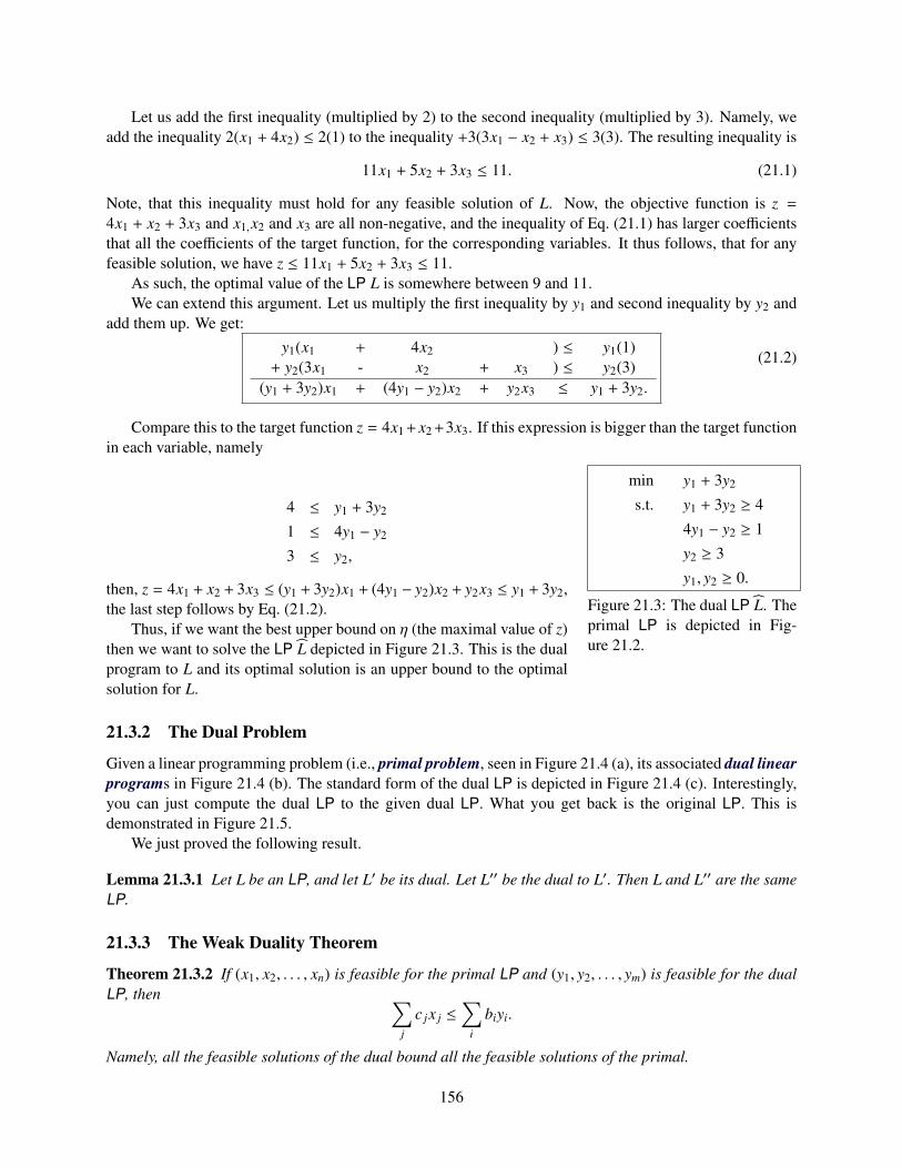
Let us add the first inequality (multiplied by 2) to the second inequality (multiplied by 3). Namely, weadd the inequality 2(x1 + 4x2) ≤ 2(1) to the inequality +3(3x1 − x2 + x3) ≤ 3(3). The resulting inequality is

11x1 + 5x2 + 3x3 ≤ 11. (21.1)

Note, that this inequality must hold for any feasible solution of L. Now, the objective function is z =4x1 + x2 + 3x3 and x1,x2 and x3 are all non-negative, and the inequality of Eq. (21.1) has larger coefficientsthat all the coefficients of the target function, for the corresponding variables. It thus follows, that for anyfeasible solution, we have z ≤ 11x1 + 5x2 + 3x3 ≤ 11.

As such, the optimal value of the LP L is somewhere between 9 and 11.We can extend this argument. Let us multiply the first inequality by y1 and second inequality by y2 and

add them up. We get:y1(x1 + 4x2 ) ≤ y1(1)+ y2(3x1 - x2 + x3 ) ≤ y2(3)

(y1 + 3y2)x1 + (4y1 − y2)x2 + y2x3 ≤ y1 + 3y2.

(21.2)

Compare this to the target function z = 4x1+ x2+3x3. If this expression is bigger than the target functionin each variable, namely

min y1 + 3y2

s.t. y1 + 3y2 ≥ 4

4y1 − y2 ≥ 1

y2 ≥ 3

y1, y2 ≥ 0.

Figure 21.3: The dual LP L. Theprimal LP is depicted in Fig-ure 21.2.

4 ≤ y1 + 3y2

1 ≤ 4y1 − y2

3 ≤ y2,

then, z = 4x1 + x2 + 3x3 ≤ (y1 + 3y2)x1 + (4y1 − y2)x2 + y2x3 ≤ y1 + 3y2,the last step follows by Eq. (21.2).

Thus, if we want the best upper bound on η (the maximal value of z)then we want to solve the LP L depicted in Figure 21.3. This is the dualprogram to L and its optimal solution is an upper bound to the optimalsolution for L.

21.3.2 The Dual Problem

Given a linear programming problem (i.e., primal problem, seen in Figure 21.4 (a), its associated dual linearprograms in Figure 21.4 (b). The standard form of the dual LP is depicted in Figure 21.4 (c). Interestingly,you can just compute the dual LP to the given dual LP. What you get back is the original LP. This isdemonstrated in Figure 21.5.

We just proved the following result.

Lemma 21.3.1 Let L be an LP, and let L′ be its dual. Let L′′ be the dual to L′. Then L and L′′ are the sameLP.

21.3.3 The Weak Duality Theorem

Theorem 21.3.2 If (x1, x2, . . . , xn) is feasible for the primal LP and (y1, y2, . . . , ym) is feasible for the dualLP, then ∑

j

c jx j ≤∑

i

biyi.

Namely, all the feasible solutions of the dual bound all the feasible solutions of the primal.

156

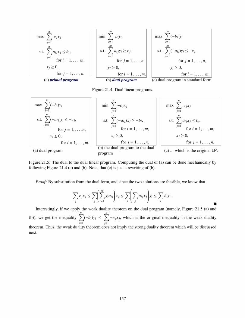
maxn∑

j=1

c jx j

s.t.n∑

j=1

ai jx j ≤ bi,

for i = 1, . . . ,m,

x j ≥ 0,

for j = 1, . . . , n.

minm∑

i=1

biyi

s.t.m∑

i=1

ai jyi ≥ c j,

for j = 1, . . . , n,

yi ≥ 0,

for i = 1, . . . ,m.

maxm∑

i=1

(−bi)yi

s.t.m∑

i=1

(−ai j)yi ≤ −c j,

for j = 1, . . . , n,

yi ≥ 0,

for i = 1, . . . ,m.(a) primal program (b) dual program (c) dual program in standard form

Figure 21.4: Dual linear programs.

maxm∑

i=1

(−bi)yi

s.t.m∑

i=1

(−ai j)yi ≤ −c j,

for j = 1, . . . , n,

yi ≥ 0,

for i = 1, . . . ,m.

minn∑

j=1

−c jx j

s.t.n∑

j=1

(−ai j)x j ≥ −bi,

for i = 1, . . . ,m,

x j ≥ 0,

for j = 1, . . . , n.

maxn∑

j=1

c jx j

s.t.n∑

j=1

ai jx j ≤ bi,

for i = 1, . . . ,m,

x j ≥ 0,

for j = 1, . . . , n.

(a) dual program(b) the dual program to the dualprogram (c) ... which is the original LP.

Figure 21.5: The dual to the dual linear program. Computing the dual of (a) can be done mechanically byfollowing Figure 21.4 (a) and (b). Note, that (c) is just a rewriting of (b).

Proof: By substitution from the dual form, and since the two solutions are feasible, we know that

∑j

c jx j ≤∑

j

m∑i=1

yiai j

x j ≤∑

i

∑j

ai jx j

yi ≤∑

i

biyi .

Interestingly, if we apply the weak duality theorem on the dual program (namely, Figure 21.5 (a) and

(b)), we get the inequalitym∑

i=1

(−bi)yi ≤

n∑j=1

−c jx j, which is the original inequality in the weak duality

theorem. Thus, the weak duality theorem does not imply the strong duality theorem which will be discussednext.

157

158

Chapter 22

Approximation Algorithms using LinearProgramming

22.1 Weighted vertex cover

Consider the Weighted Vertex Cover problem. Here, we have a graph G = (V,E), and furthermore eachvertex v ∈ V has a cost cv. We would like to compute a vertex cover of minimum cost – a subset of thevertices of G with minimum total cost so that each edge has at least one of its endpoints in the cover. Thisproblem is (of course) NP-H, since the decision problem where all the weights are 1, is the Vertex Coverproblem, which we had shown to be NPC.

Let us first state this optimization problem is an integer programming. Indeed, for any v ∈ V, let definea variable xv which is 1 if we decide to pick v to the vertex cover, and zero otherwise. The fact that xv isrestricted to be either 0 or 1, we will write formally as xv ∈ 0, 1. Next, we will require that every edgevu ∈ E is covered. Namely, we require that xv ∨ xu to be TRUE. For reasons that would be come clearershortly, we prefer to write this condition as a linear inequality; namely, we require that xv + xu ≥ 1. Finally,we would like to minimize the total cost of the vertices we pick for the cover; namely, we would like tominimize

∑v∈V xvcv. Putting it together, we get the following integer programming instance:

min∑v∈V

cvxv,

such that ∀v ∈ V xv ∈ 0, 1 , (22.1)

∀vu ∈ E xv + xu ≥ 1.

Naturally, solving this integer programming efficiently is NP-H, so instead let us try to relax thisoptimization problem to be a LP (which we can solve efficiently, at least in practice). To do this, we needto relax the integer program. We will do it by allowing the variables xv to get real values between 0 and 1.This is done by replacing the condition that xv ∈ 0, 1 by the constraint 0 ≤ xv ≤ 1. The resulting LP is

min∑v∈V

cvxv, (22.2)

such that ∀v ∈ V 0 ≤ xv,

∀v ∈ V xv ≤ 1, (22.3)

∀vu ∈ E xv + xu ≥ 1.

And also in theory if the costs are integers, using more advanced algorithms than the Simplex algorithm.

159

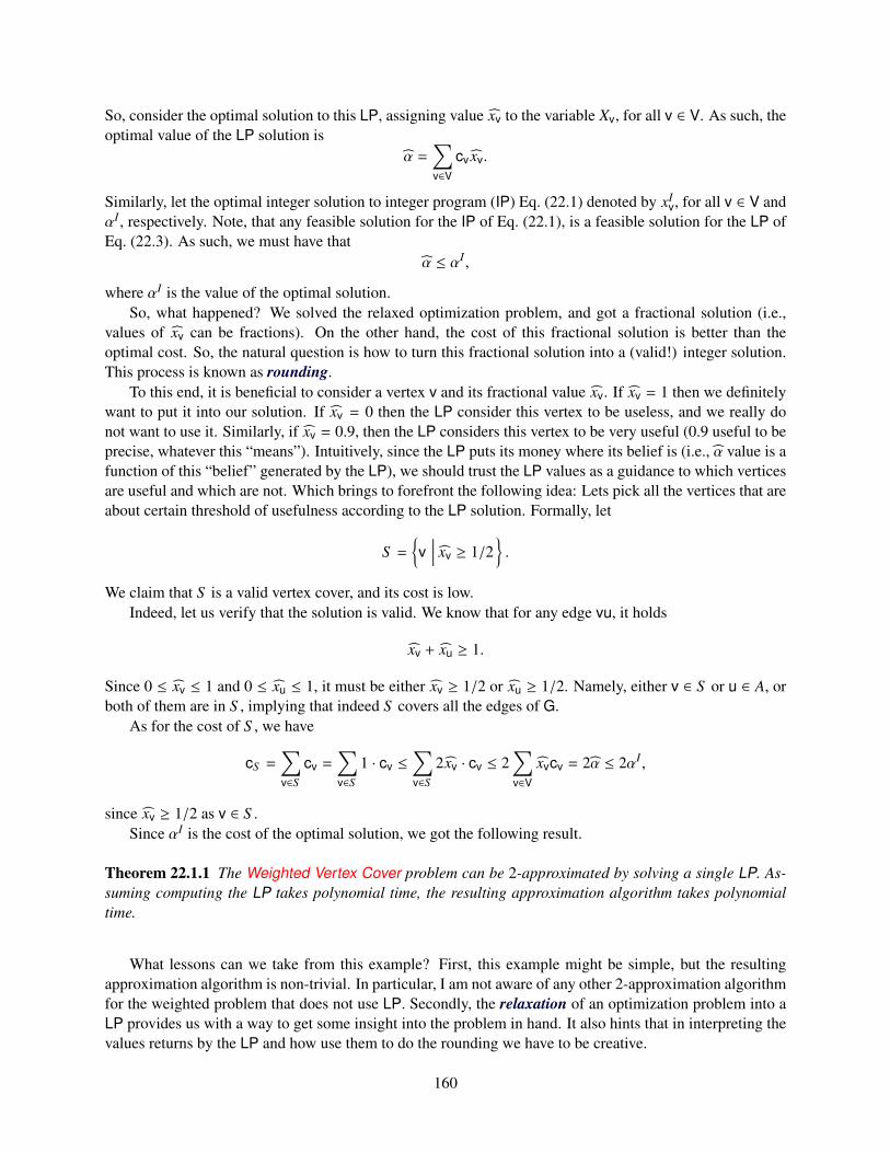
So, consider the optimal solution to this LP, assigning value xv to the variable Xv, for all v ∈ V. As such, theoptimal value of the LP solution is

α =∑v∈V

cv xv.

Similarly, let the optimal integer solution to integer program (IP) Eq. (22.1) denoted by xIv, for all v ∈ V and

αI , respectively. Note, that any feasible solution for the IP of Eq. (22.1), is a feasible solution for the LP ofEq. (22.3). As such, we must have that

α ≤ αI ,

where αI is the value of the optimal solution.So, what happened? We solved the relaxed optimization problem, and got a fractional solution (i.e.,

values of xv can be fractions). On the other hand, the cost of this fractional solution is better than theoptimal cost. So, the natural question is how to turn this fractional solution into a (valid!) integer solution.This process is known as rounding.

To this end, it is beneficial to consider a vertex v and its fractional value xv. If xv = 1 then we definitelywant to put it into our solution. If xv = 0 then the LP consider this vertex to be useless, and we really donot want to use it. Similarly, if xv = 0.9, then the LP considers this vertex to be very useful (0.9 useful to beprecise, whatever this “means”). Intuitively, since the LP puts its money where its belief is (i.e., α value is afunction of this “belief” generated by the LP), we should trust the LP values as a guidance to which verticesare useful and which are not. Which brings to forefront the following idea: Lets pick all the vertices that areabout certain threshold of usefulness according to the LP solution. Formally, let

S =v

∣∣∣∣ xv ≥ 1/2.

We claim that S is a valid vertex cover, and its cost is low.Indeed, let us verify that the solution is valid. We know that for any edge vu, it holds

xv + xu ≥ 1.

Since 0 ≤ xv ≤ 1 and 0 ≤ xu ≤ 1, it must be either xv ≥ 1/2 or xu ≥ 1/2. Namely, either v ∈ S or u ∈ A, orboth of them are in S , implying that indeed S covers all the edges of G.

As for the cost of S , we have

cS =∑v∈S

cv =∑v∈S

1 · cv ≤∑v∈S

2xv · cv ≤ 2∑v∈V

xvcv = 2α ≤ 2αI ,

since xv ≥ 1/2 as v ∈ S .Since αI is the cost of the optimal solution, we got the following result.

Theorem 22.1.1 The Weighted Vertex Cover problem can be 2-approximated by solving a single LP. As-suming computing the LP takes polynomial time, the resulting approximation algorithm takes polynomialtime.

What lessons can we take from this example? First, this example might be simple, but the resultingapproximation algorithm is non-trivial. In particular, I am not aware of any other 2-approximation algorithmfor the weighted problem that does not use LP. Secondly, the relaxation of an optimization problem into aLP provides us with a way to get some insight into the problem in hand. It also hints that in interpreting thevalues returns by the LP and how use them to do the rounding we have to be creative.

160

22.2 Revisiting Set Cover

In this section, we are going to revisit the Set Cover problem, and provide an approximation algorithm forthis problem. This approximation algorithm would not be better than the greedy algorithm we already saw,but it would expose us to a new technique that we would use shortly for a different problem.

Problem: Set Cover

Instance: (S ,F )S - a set of n elementsF - a family of subsets of S , s.t.

⋃X∈F X = S .

Output: The set X ⊆ F such that X contains as few sets as possible, and Xcovers S .

As before, we will first define an IP for this problem. In the following IP, the second condition just statesthat any s ∈ s, must be covered by some set.

∀U ∈ F xU ∈ 0, 1 ,

∀s ∈ S∑

U∈F,s∈U

xU ≥ 1

min α =∑U∈F

xU ,

Next, we relax this IP into the following LP.

∀U ∈ F 0 ≤ xU ≤ 1,

∀s ∈ S∑

U∈F,s∈U

xU ≥ 1

min α =∑U∈F

xU ,

As before, consider the optimal solution to the LP: ∀U ∈ F, xU , and α. Similarly, let the optimal solutionto the IP (and thus for the problem) be: ∀U ∈ F, xI

U , and αI . As before, we would try to use the LP solutionto guide us in the rounding process. As before, if xU is close to 1 then we should pick U to the cover and ifxU is close to 0 we should not. As such, its natural to pick U ∈ F into the cover by randomly choosing itinto the cover with probability xU . Consider the resulting family of sets G. Let ZS be an indicator variablewhich is one if S ∈ G. We have that the cost of G is

∑S∈F ZS , and the expected cost is

E[cost of G

]= E

∑S∈F

ZS

=∑S∈F

E[ZS

]=

∑S∈F

Pr[S ∈ G

]=

∑S∈F

xS = α ≤ αI . (22.4)

As such, in expectation, G is not too expensive. The problem, of course, is that G might fail to cover someelement s ∈ S . To this end, we repeat this algorithm m = O(log n) times, where n = |S |. Let Gi be therandom cover computed in the ith iteration, and let H = ∪iGi. We return H as the required cover.

The solution H covers S . For an element s ∈ S , we have that∑U∈F,s∈U

xU ≥ 1, . (22.5)

161

and consider the probability that s is not covered by Gi, where Gi is the family computed in the ith iterationof the algorithm. Since deciding if the include each set U into Gi is done independently for each set, wehave that the probability that s is not covered is

Pr[s not covered by Gi

]= Pr

[none of U ∈ F, such that s ∈ U were picked into Gi

]=

∏U∈F,s∈U

Pr[U was not picked into Gi

]=

∏U∈F,s∈U

(1 − xU

)≤

∏U∈F,s∈U

exp(−xU

)= exp

− ∑U∈F,s∈U

xU

≤ exp(−1) ≤

12,

by Eq. (22.5). As such, the probability that s is not covered in all m iterations is at most(12

)m

<1

n10 ,

since m = O(log n). In particular, the probability that one of the n elements of S is not covered by H is atmost n(1/n10) = 1/n9.

Cost. By Eq. (22.4), in each iteration the expected cost of the cover computed is at most the cost of theoptimal solution (i.e., αI). As such the expected cost of the solution computed is

cH ≤∑

i

cBi ≤ mαI = O(αI log n

).

. Putting everything together, we get the following result.

Theorem 22.2.1 By solving an LP one can get an O(log n)-approximation to set cover by a randomizedalgorithm. The algorithm succeeds with high probability.

22.3 Minimizing congestion

Let G be a graph with n vertices, and let πi and σi be two paths with the same endpoints vi, ui ∈ V(G), fori = 1, . . . , t. Imagine that we need to send one unit of flow from vi to ui, and we need to choose whether touse the path πi or σi. We would like to do it in such a way that not edge in the graph is being used too much.

Definition 22.3.1 Given a set X of paths in a graph G, the congestion of X is the maximum number of pathsin X that use the same edge.

Consider the following linear program:

min w

xi ≥ 0

xi ≤ 1

∀e ∈ E∑e∈πi

xi +∑e∈σi

(1 − xi) ≤ w

162

Let xi be the value of xi in the optimal solution to this LP, and let w be the value of w in this solution.Clearly, the optimal congestion must be bigger than w.

Let Xi be a random variable which is one with probability xi, and zero otherwise. If Xi = 1 then we useπ to route from vi to ui, otherwise we use σi. Clearly, the congestion of e is

Ye =∑e∈πi

Xi +∑e∈σi

(1 − Xi).

And in expectation

αe = E[Ye] = E

∑e∈πi

Xi +∑e∈σi

(1 − Xi)

=∑e∈πi

E[Xi] +∑e∈σi

E[(1 − Xi)] =∑e∈πi

xi +∑e∈σi

(1 − xi) ≤ w.

Using the Chernoff inequality, we have that

Pr[Ye ≥ (1 + δ)αe] ≤ exp(−αeδ

2

4

)≤ exp

(−

wδ2

4

).

(Note, that this works only if δ < 2e − 1, see Theorem 10.2.7.) Let δ =

√20w

ln t. We have that

Pr[Ye ≥ (1 + δ)αe] ≤≤ exp(−δ2

4

)≤

1t100 ,

which is very small. In particular, if t ≥ n1/50 then all the edges in the graph do not have congestion largerthan (1 + δ)w.

To see what this result means, let us play with the numbers. Let assume that t = n, and w ≥√

n. Then,the solution has congestion larger than the optimal solution by a factor of

1 + δ = 1 +

√20w

ln t ≤= 1 +

√20 ln nn1/4 ,

which is of course extremely close to 1, if n is sufficiently larger.

Theorem 22.3.2 Given a graph with n vertices, and t pairs of vertices, such that for every pair (si, ti) thereare two possible paths to connect si to ti. Then one can choose for each pair which path to use, such thatthe most congested edge, would have at most (1+ δ)opt, where opt is the congestion of the optimal solution,

and δ =√

20w ln t.

When the congestion is low. Assume that w is a constant. In this case, we can get a better bound by usingthe Chernoff inequality its more general form, see Theorem 10.2.7. Indeed, set δ = c ln t/ ln ln t, where c isa constant. For µ = αe, we have that

Pr[Ye ≥ (1 + δ)µ

]≤

(eδ

(1 + δ)1+δ

)µ. = exp

µ(δ − (1 + δ) ln(1 + δ)) = exp

− µc′ ln t

≤ 1tO(1) ,

where c′ is a constant that depends on c and grows if c grows. We just proved that if the optimal congestionis O(1), then the algorithm outputs a solution with congestion O(log t/ log log t), and this holds with highprobability.

163

164

Part IX

Approximate Max Cut

165

Chapter 23

Approximate Max Cut

23.1 Problem Statement

Given an undirected graph G = (V,E) and nonnegative weights ωi j on the edge i j ∈ E, the maximum cutproblem (MAX CUT) is that of finding the set of vertices S that maximizes the weight of the edges in the cut(S , S ); that is, the weight of the edges with one endpoint in S and the other in S . For simplicity, we usuallyset ωi j = O for i j < E and denote the weight of a cut (S , S ) by w(S , S ) =

∑i∈S , j∈S

ωi j.

This problem is NP-C, and hard to approximate within a certain constant.Given a graph with vertex set V = 1, . . . , n and nonnegative weights ωi j, the weight of the maximum

cut w(S , S ) is given by the following integer quadratic program:

(Q) max12

∑i< j

ωi j(1 − yiy j)

subject to: yi ∈ −1, 1 ∀i ∈ V.

Indeed, set S =i∣∣∣∣ yi = 1

. Clearly, ω

(S , S

)= 1

2∑

i< j, ωi j(1 − yiy j).

Solving quadratic integer programming is of course NP-H. Thus, we will relax it, by thinking aboutthe numbers yi as unit vectors in higher dimensional space. If so, the multiplication of the two vectors, isnow replaced by dot product. We have:

(Q) max12

∑i< j

ωi j(1 −

⟨vi, v j

⟩)subject to: vi ∈ S

(n) ∀i ∈ V,

where S(n) is the n dimensional unit sphere in IRn+1. This is an instance of semi-definite programming,which is a special case of convex programming, which can be solved in polynomial time (solved here meansapproximated within arbitrary constant in polynomial time). Observe that (P) is a relaxation of (Q), and assuch the optimal solution of (P) has value larger than the optimal value of (Q).

The intuition is that vectors that correspond to vertices that should be on one side of the cut, and verticeson the other sides, would have vectors which are faraway from each other in (P). Thus, we compute theoptimal solution for (P), and we uniformly generate a random vector ~r on the unit sphere S(n). This inducesa hyperplane h which passes through the origin and is orthogonal to ~r. We next assign all the vectors thatare on one side of h to S , and the rest to S .

167

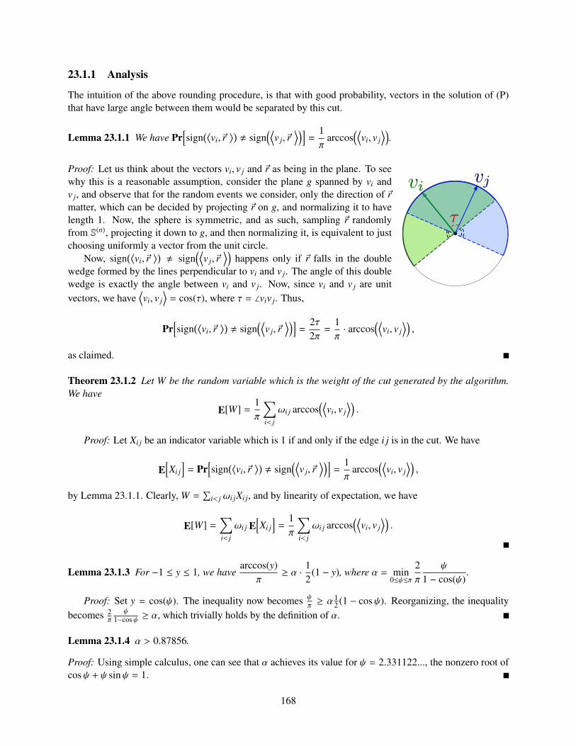
23.1.1 Analysis

The intuition of the above rounding procedure, is that with good probability, vectors in the solution of (P)that have large angle between them would be separated by this cut.

Lemma 23.1.1 We have Pr[sign

(⟨vi,~r

⟩), sign

(⟨v j,~r

⟩)]=

1π

arccos(⟨

vi, v j⟩)

.

Proof: Let us think about the vectors vi, v j and ~r as being in the plane. To seewhy this is a reasonable assumption, consider the plane g spanned by vi andv j, and observe that for the random events we consider, only the direction of ~rmatter, which can be decided by projecting ~r on g, and normalizing it to havelength 1. Now, the sphere is symmetric, and as such, sampling ~r randomlyfrom S(n), projecting it down to g, and then normalizing it, is equivalent to justchoosing uniformly a vector from the unit circle.

Now, sign(⟨

vi,~r⟩), sign

(⟨v j,~r

⟩)happens only if ~r falls in the double

wedge formed by the lines perpendicular to vi and v j. The angle of this doublewedge is exactly the angle between vi and v j. Now, since vi and v j are unitvectors, we have

⟨vi, v j

⟩= cos(τ), where τ = ∠viv j. Thus,

Pr[sign

(⟨vi,~r

⟩), sign

(⟨v j,~r

⟩)]=

2τ2π=

1π· arccos

(⟨vi, v j

⟩),

as claimed.

Theorem 23.1.2 Let W be the random variable which is the weight of the cut generated by the algorithm.We have

E[W] =1π

∑i< j

ωi j arccos(⟨

vi, v j⟩).

Proof: Let Xi j be an indicator variable which is 1 if and only if the edge i j is in the cut. We have

E[Xi j

]= Pr

[sign

(⟨vi,~r

⟩), sign

(⟨v j,~r

⟩)]=

1π

arccos(⟨

vi, v j⟩),

by Lemma 23.1.1. Clearly, W =∑

i< j ωi jXi j, and by linearity of expectation, we have

E[W] =∑i< j

ωi j E[Xi j

]=

1π

∑i< j

ωi j arccos(⟨

vi, v j⟩).

Lemma 23.1.3 For −1 ≤ y ≤ 1, we havearccos(y)

π≥ α ·

12

(1 − y), where α = min0≤ψ≤π

2π

ψ

1 − cos(ψ).

Proof: Set y = cos(ψ). The inequality now becomes ψπ ≥ α

12 (1 − cosψ). Reorganizing, the inequality

becomes 2π

ψ1−cosψ ≥ α, which trivially holds by the definition of α.

Lemma 23.1.4 α > 0.87856.

Proof: Using simple calculus, one can see that α achieves its value for ψ = 2.331122..., the nonzero root ofcosψ + ψ sinψ = 1.

168

Theorem 23.1.5 The above algorithm computes in expectation a cut with total weight α·Opt ≥ 0.87856Opt,where Opt is the weight of the maximal cut.

Proof: Consider the optimal solution to (P), and lets its value be γ ≥ Opt. We have

E[W] =1π

∑i< j

ωi j arccos(⟨

vi, v j⟩)≥

∑i< j

ωi jα12

(1 −

⟨vi, v j

⟩)= αγ ≥ α · Opt,

by Lemma 23.1.3.

23.2 Semi-definite programming

Let us define a variable xi j =⟨vi, v j

⟩, and consider the n by n matrix M formed by those variables, where

xii = 1 for i = 1, . . . , n. Let V be the matrix having v1, . . . , vn as its columns. Clearly, M = VT V . Inparticular, this implies that for any non-zero vector v ∈ IRn, we have vT Mv = vT AT Av = (Av)T (Av) ≥ 0. Amatrix that has this property, is called positive semidefinite. Interestingly, any positive semidefinite matrixP can be represented as a product of a matrix with its transpose; namely, P = BT B. Furthermore, given sucha matrix P of size n × n, we can compute B such that P = BT B in O(n3) time. This is know as Choleskydecomposition.

Observe, that if a semidefinite matrix P = BT B has a diagonal where all the entries are one, then B hascolumns which are unit vectors. Thus, if we solve (P) and get back a semi-definite matrix, then we canrecover the vectors realizing the solution, and use them for the rounding.

In particular, (P) can now be restated as

(S D) max12

∑i< j

ωi j(1 − xi j)

subject to: xii = 1 for i = 1, . . . , n(xi j

)i=1,...,n, j=1,...,n

is a positive semi-definite matrix.

We are trying to find the optimal value of a linear function over a set which is the intersection of linearconstraints and the set of positive semi-definite matrices.

Lemma 23.2.1 Let U be the set of n × n positive semidefinite matrices. The set U is convex.

Proof: Consider A, B ∈ U, and observe that for any t ∈ [0, 1], and vector v ∈ IRn, we have:

vT(tA + (1 − t)B

)v = vT

(tAv + (1 − t)Bv

)= tvT Av + (1 − t)vT Bv ≥ 0 + 0 ≥ 0,

since A and B are positive semidefinite.

Positive semidefinite matrices corresponds to ellipsoids. Indeed, consider the set xT Ax = 1: the setof vectors that solve this equation is an ellipsoid. Also, the eigenvalues of a positive semidefinite matrixare all non-negative real numbers. Thus, given a matrix, we can in polynomial time decide if it is positivesemidefinite or not (by computing the eigenvalues of the matrix).

Thus, we are trying to optimize a linear function over a convex domain. There is by now machinery toapproximately solve those problems to within any additive error in polynomial time. This is done by usingthe interior point method, or the ellipsoid method. See [BV04, GLS88] for more details. The key ingredientthat is required to make these methods work, is the ability to decide in polynomial time, given a solution,whether its feasible or not. As demonstrated above, this can be done in polynomial time.

169


The approximation algorithm presented is from the work of Goemans and Williamson [GW95]. Håstad[Hås01] showed that MAX CUT can not be approximated within a factor of 16/17 ≈ 0.941176. Recently,Khot et al. [KKMO04] showed a hardness result that matches the constant of Goemans and Williamson(i.e., one can not approximate it better than α, unless P = NP). However, this relies on two conjectures, thefirst one is the “Unique Games Conjecture”, and the other one is “Majority is Stablest”. The “Majority isStablest” conjecture was recently proved by Mossel et al. [MOO05]. However, it is not clear if the “UniqueGames Conjecture” is true, see the discussion in [KKMO04].

The work of Goemans and Williamson was very influential and spurred wide research on using SDP forapproximation algorithms. For an extension of the MAX CUT problem where negative weights are allowedand relevant references, see the work by Alon and Naor [AN04].

170

Part X

Learning and Linear Separability

171

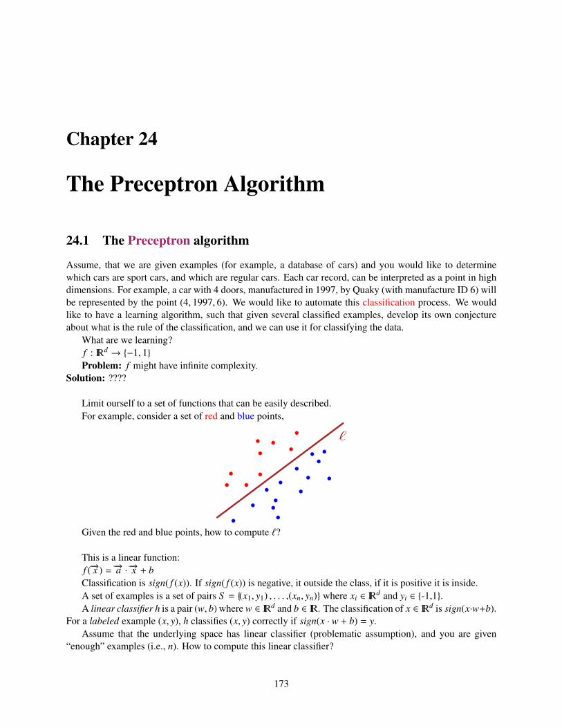
Chapter 24

The Preceptron Algorithm

24.1 The Preceptron algorithm

Assume, that we are given examples (for example, a database of cars) and you would like to determinewhich cars are sport cars, and which are regular cars. Each car record, can be interpreted as a point in highdimensions. For example, a car with 4 doors, manufactured in 1997, by Quaky (with manufacture ID 6) willbe represented by the point (4, 1997, 6). We would like to automate this classification process. We wouldlike to have a learning algorithm, such that given several classified examples, develop its own conjectureabout what is the rule of the classification, and we can use it for classifying the data.

What are we learning?f : IRd → −1, 1Problem: f might have infinite complexity.

Solution: ????

Limit ourself to a set of functions that can be easily described.For example, consider a set of red and blue points,

`

Given the red and blue points, how to compute `?

This is a linear function:f (−→x ) = −→a · −→x + bClassification is sign( f (x)). If sign( f (x)) is negative, it outside the class, if it is positive it is inside.A set of examples is a set of pairs S = (x1, y1) , . . . ,(xn, yn) where xi ∈ IRd and yi ∈ -1,1.A linear classifier h is a pair (w, b) where w ∈ IRd and b ∈ IR. The classification of x ∈ IRd is sign(x·w+b).

For a labeled example (x, y), h classifies (x, y) correctly if sign(x · w + b) = y.Assume that the underlying space has linear classifier (problematic assumption), and you are given

“enough” examples (i.e., n). How to compute this linear classifier?

173

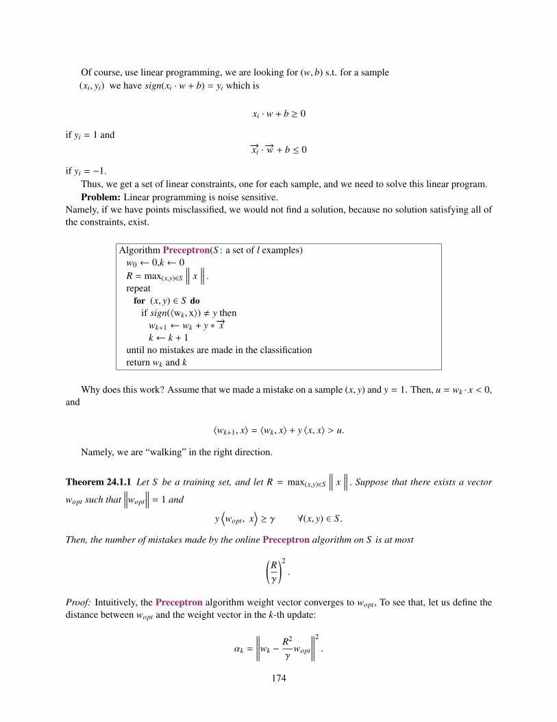
Of course, use linear programming, we are looking for (w, b) s.t. for a sample(xi, yi) we have sign(xi · w + b) = yi which is

xi · w + b ≥ 0

if yi = 1 and−→xi ·−→w + b ≤ 0

if yi = −1.Thus, we get a set of linear constraints, one for each sample, and we need to solve this linear program.Problem: Linear programming is noise sensitive.

Namely, if we have points misclassified, we would not find a solution, because no solution satisfying all ofthe constraints, exist.

Algorithm Preceptron(S : a set of l examples)w0 ← 0,k ← 0R = max(x,y)∈S

∥∥∥∥ x∥∥∥∥ .

repeatfor (x, y) ∈ S do

if sign(〈wk, x〉) , y thenwk+1 ← wk + y ∗ −→xk ← k + 1

until no mistakes are made in the classificationreturn wk and k

Why does this work? Assume that we made a mistake on a sample (x, y) and y = 1. Then, u = wk · x < 0,and

〈wk+1, x〉 = 〈wk, x〉 + y 〈x, x〉 > u.

Namely, we are “walking” in the right direction.

Theorem 24.1.1 Let S be a training set, and let R = max(x,y)∈S

∥∥∥∥ x∥∥∥∥ . Suppose that there exists a vector

wopt such that∥∥∥∥wopt

∥∥∥∥ = 1 and

y⟨wopt, x

⟩≥ γ ∀(x, y) ∈ S .

Then, the number of mistakes made by the online Preceptron algorithm on S is at most(Rγ

)2

.

Proof: Intuitively, the Preceptron algorithm weight vector converges to wopt, To see that, let us define thedistance between wopt and the weight vector in the k-th update:

αk =

∥∥∥∥∥∥wk −R2

γwopt

∥∥∥∥∥∥2

.

174

We next quantify the change between αk and αk+1 (the example being misclassified is (x, y)):

αk+1 =

∥∥∥∥∥∥wk+1 −R2

γwopt

∥∥∥∥∥∥2

=

∥∥∥∥∥∥wk + yx −R2

γwopt

∥∥∥∥∥∥2

=

∥∥∥∥∥∥(wk −

R2

γwopt

)+ yx

∥∥∥∥∥∥2

=

⟨(wk −

R2

γwopt

)+ yx ,

(wk −

R2

γwopt

)+ yx

⟩.

Expanding this we get:

αk+1 =

⟨(wk −

R2

γwopt

),

(wk −

R2

γwopt

)⟩+2y

⟨(wk −

R2

γwopt

), x

⟩+ 〈x, x〉

= αk + 2y⟨(

wk −R2

γwopt

), x

⟩+

∥∥∥∥ x∥∥∥∥2.

Since ||x|| ≤ R,we have

αk+1 ≤ αk + R2 + 2y 〈wk, x〉 − 2y⟨

R2

γwopt, x

⟩≤ αk + R2 + −2

R2

γy⟨wopt,x

⟩.

Next, since y⟨wopt , x

⟩≥ γ for ∀(x, y) ∈ S , we have that

αk+1 ≤ αk + R2 − 2R2

γγ

≤ αk + R2 − 2R2

≤ αk − R2.

We have: αk+1 ≤ αk − R2, and

α0 =

∥∥∥∥∥∥0 −R2

γwopt

∥∥∥∥∥∥2

=R4

γ2

∥∥∥∥wopt

∥∥∥∥2=

R4

γ2 .

Finally, observe that αi ≥ 0 for all i. Thus, what is the maximum number of classification errors thealgorithm can make? (

R2

γ2

).

It is important to observe that any linear program can be written as the problem of seperating red pointsfrom blue points. As such, the Preceptron algorithm can be used to solve sovle linear programs...

175

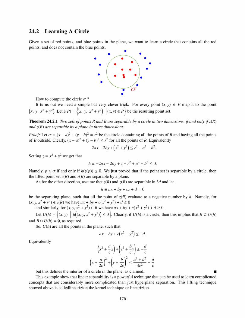
24.2 Learning A Circle

Given a set of red points, and blue points in the plane, we want to learn a circle that contains all the redpoints, and does not contain the blue points.

σ

How to compute the circle σ ?It turns out we need a simple but very clever trick. For every point (x, y) ∈ P map it to the point(

x, y, x2 + y2). Let z(P) =

(x, y, x2 + y2

) ∣∣∣∣ (x, y) ∈ P

be the resulting point set.

Theorem 24.2.1 Two sets of points R and B are separable by a circle in two dimensions, if and only if z(R)and z(B) are separable by a plane in three dimensions.

Proof: Let σ ≡ (x − a)2 + (y − b)2 = r2 be the circle containing all the points of R and having all the pointsof B outside. Clearly, (x − a)2 + (y − b)2 ≤ r2 for all the points of R. Equivalently

−2ax − 2by +(x2 + y2

)≤ r2 − a2 − b2.

Setting z = x2 + y2 we get that

h ≡ −2ax − 2by + z − r2 + a2 + b2 ≤ 0.

Namely, p ∈ σ if and only if h(z(p)) ≤ 0. We just proved that if the point set is separable by a circle, thenthe lifted point set z(R) and z(B) are separable by a plane.

As for the other direction, assume that z(R) and z(B) are separable in 3d and let

h ≡ ax + by + cz + d = 0

be the separating plane, such that all the point of z(R) evaluate to a negative number by h. Namely, for(x, y, x2 + y2) ∈ z(R) we have ax + by + c(x2 + y2) + d ≤ 0

and similarly, for (x, y, x2 + y2) ∈ B we have ax + by + c(x2 + y2) + d ≥ 0.

Let U(h) =(x, y)

∣∣∣∣ h((x, y, x2 + y2)

)≤ 0

. Clearly, if U(h) is a circle, then this implies that R ⊂ U(h)

and B ∩ U(h) = ∅, as required.So, U(h) are all the points in the plane, such that

ax + by + c(x2 + y2

)≤ −d.

Equivalently (x2 +

ac

x)+

(y2 +

bc

y)≤ −

dc(

x +a2c

)2+

(y +

b2c

)2

≤a2 + b2

4c2 −dc

but this defines the interior of a circle in the plane, as claimed.This example show that linear separability is a powerful technique that can be used to learn complicated

concepts that are considerably more complicated than just hyperplane separation. This lifting techniqueshowed above is calledlinearizion the kernel technique or linearizion.

176

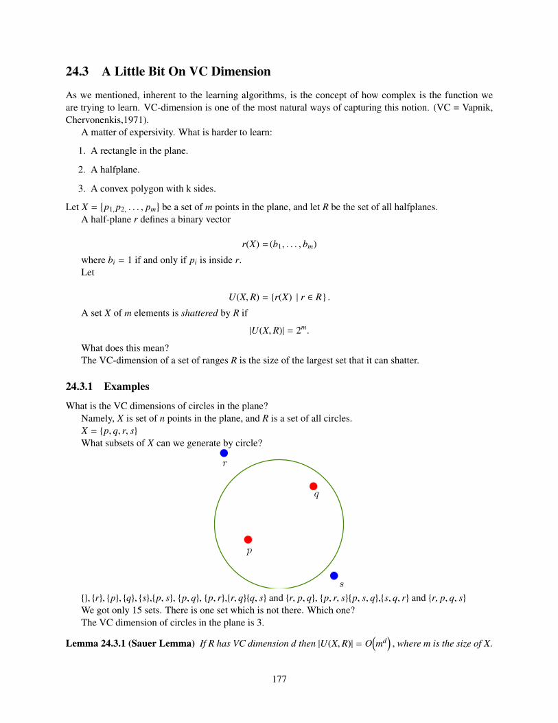
24.3 A Little Bit On VC Dimension

As we mentioned, inherent to the learning algorithms, is the concept of how complex is the function weare trying to learn. VC-dimension is one of the most natural ways of capturing this notion. (VC = Vapnik,Chervonenkis,1971).

A matter of expersivity. What is harder to learn:

1. A rectangle in the plane.

2. A halfplane.

3. A convex polygon with k sides.

Let X =p1,p2, . . . , pm

be a set of m points in the plane, and let R be the set of all halfplanes.

A half-plane r defines a binary vector

r(X) = (b1, . . . , bm)

where bi = 1 if and only if pi is inside r.Let

U(X,R) = r(X) | r ∈ R .

A set X of m elements is shattered by R if

|U(X,R)| = 2m.

What does this mean?The VC-dimension of a set of ranges R is the size of the largest set that it can shatter.

24.3.1 Examples

What is the VC dimensions of circles in the plane?Namely, X is set of n points in the plane, and R is a set of all circles.X = p, q, r, sWhat subsets of X can we generate by circle?

p

q

r

s

, r, p, q, s,p, s, p, q, p, r,r, qq, s and r, p, q, p, r, sp, s, q,s, q, r and r, p, q, sWe got only 15 sets. There is one set which is not there. Which one?The VC dimension of circles in the plane is 3.

Lemma 24.3.1 (Sauer Lemma) If R has VC dimension d then |U(X,R)| = O(md

), where m is the size of X.

177

178

Part XI

Compression, Information and Entropy

179

Chapter 25

Huffman Coding

25.1 Huffman coding

(This portion of the class notes is based on Jeff Erickson class notes.)A binary code assigns a string of 0s and 1s to each character in the alphabet. A code assigns for each

symbol in the input a codeword over some other alphabet. Such a coding is necessary, for example, fortransmitting messages over a wire, were you can send only 0 or 1 on the wire (i.e., for example, considerthe good old telegraph and Morse code). The receiver gets a binary stream of bits and needs to decode themessage sent. A prefix code, is a code where one can decipher the message, a character by character, by justreading a prefix of the input binary string, matching it to an original character, and continuing to decipherthe rest of the stream. Such a code is known as a prefix code.

A binary code (or a prefix code) is prefix-free if no code is a prefix of any other. ASCII and Unicode’sUTF-8 are both prefix-free binary codes. Morse code is a binary code (and also a prefix code), but it is notprefix-free; for example, the code for S (· · · ) includes the code for E (·) as a prefix. (Hopefully the receiverknows that when it gets · · · that it is extremely unlikely that this should be interpreted as EEE, but ratherS. Any prefix-free binary code can be visualized as a binary tree with the encoded characters stored at theleaves. The code word for any symbol is given by the path from the root to the corresponding leaf; 0 forleft, 1 for right. The length of a codeword for a symbol is the depth of the corresponding leaf. Such treesare usually referred to as prefix trees or code treestree!code trees.

a

b c

d0

0

0

1

1

1The beauty of prefix trees (and thus of prefix odes) is that decoding is very easy.As a concrete example, consider the tree on the right. Given a string ’010100’, wecan traverse down the tree from the root, going left if get a ’0’ and right if we get’1’. Whenever we get to a leaf, we output the character output in the leaf, and wejump back to the root for the next character we are about to read. For the example’010100’, after reading ’010’ our traversal in the tree leads us to the leaf markedwith ’b’, we jump back to the root and read the next input digit, which is ’1’, andthis leads us to the leaf marked with ’d’, which we output, and jump back to the root. Finally, ’00’ leads usto the leaf marked by ’a’, which the algorithm output. Thus, the binary string ’010100’ encodes the string“bda”.

Suppose we want to encode messages in an n-character alphabet so that the encoded message is as shortas possible. Specifically, given an array frequency counts f [1 . . . n], we want to compute a prefix-free binarycode that minimizes the total encoded length of the message. That is we would like to compute a tree T thatminimizes

cost(T) =n∑

i=1

f [i] ∗ len(code(i)) , (25.1)

181

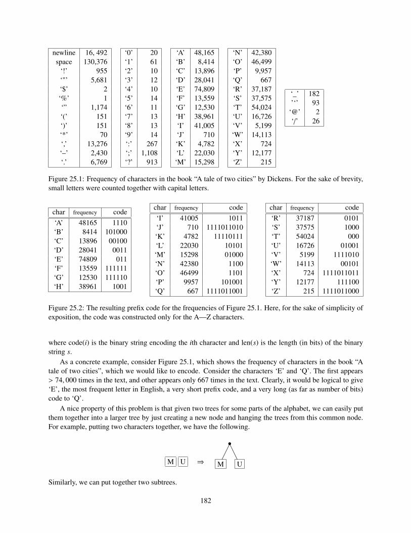
newline 16, 492space 130,376

‘!’ 955‘"’ 5,681‘$’ 2‘%’ 1‘” 1,174‘(’ 151‘)’ 151‘*’ 70‘,’ 13,276‘–’ 2,430‘.’ 6,769

‘0’ 20‘1’ 61‘2’ 10‘3’ 12‘4’ 10‘5’ 14‘6’ 11‘7’ 13‘8’ 13‘9’ 14‘:’ 267‘;’ 1,108‘?’ 913

‘A’ 48,165‘B’ 8,414‘C’ 13,896‘D’ 28,041‘E’ 74,809‘F’ 13,559‘G’ 12,530‘H’ 38,961‘I’ 41,005‘J’ 710‘K’ 4,782‘L’ 22,030‘M’ 15,298

‘N’ 42,380‘O’ 46,499‘P’ 9,957‘Q’ 667‘R’ 37,187‘S’ 37,575‘T’ 54,024‘U’ 16,726‘V’ 5,199‘W’ 14,113‘X’ 724‘Y’ 12,177‘Z’ 215

‘_’ 182’‘’ 93

‘@’ 2‘/’ 26

Figure 25.1: Frequency of characters in the book “A tale of two cities” by Dickens. For the sake of brevity,small letters were counted together with capital letters.

char frequency code‘A’ 48165 1110‘B’ 8414 101000‘C’ 13896 00100‘D’ 28041 0011‘E’ 74809 011‘F’ 13559 111111‘G’ 12530 111110‘H’ 38961 1001

char frequency code‘I’ 41005 1011‘J’ 710 1111011010‘K’ 4782 11110111‘L’ 22030 10101‘M’ 15298 01000‘N’ 42380 1100‘O’ 46499 1101‘P’ 9957 101001‘Q’ 667 1111011001

char frequency code‘R’ 37187 0101‘S’ 37575 1000‘T’ 54024 000‘U’ 16726 01001‘V’ 5199 1111010‘W’ 14113 00101‘X’ 724 1111011011‘Y’ 12177 111100‘Z’ 215 1111011000

Figure 25.2: The resulting prefix code for the frequencies of Figure 25.1. Here, for the sake of simplicity ofexposition, the code was constructed only for the A—Z characters.

where code(i) is the binary string encoding the ith character and len(s) is the length (in bits) of the binarystring s.

As a concrete example, consider Figure 25.1, which shows the frequency of characters in the book “Atale of two cities”, which we would like to encode. Consider the characters ‘E’ and ‘Q’. The first appears> 74, 000 times in the text, and other appears only 667 times in the text. Clearly, it would be logical to give‘E’, the most frequent letter in English, a very short prefix code, and a very long (as far as number of bits)code to ‘Q’.

A nice property of this problem is that given two trees for some parts of the alphabet, we can easily putthem together into a larger tree by just creating a new node and hanging the trees from this common node.For example, putting two characters together, we have the following.

M U ⇒

•

M

.................................................................

U

................................................................

Similarly, we can put together two subtrees.

182

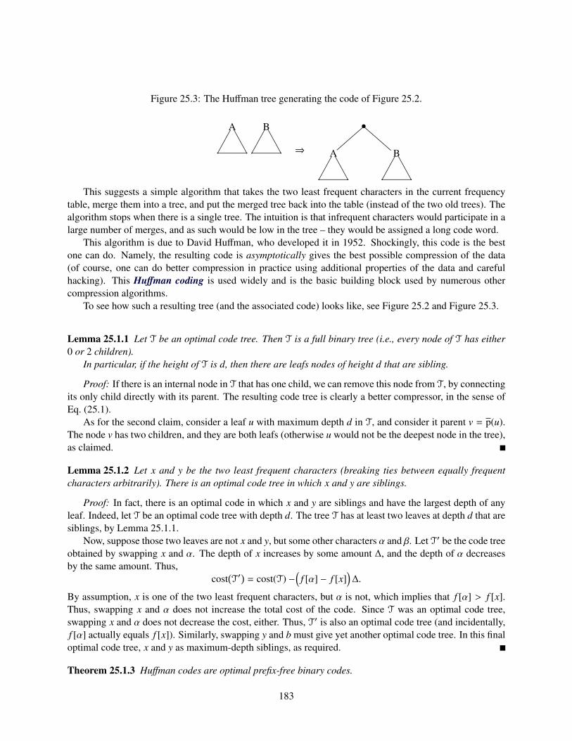
Figure 25.3: The Huffman tree generating the code of Figure 25.2.

A

.

..................................................................... .

...................................................................................................................................................

B

.

..................................................................... .

................................................................................................................................................... ⇒

•

A

.

..................................................................... .

...................................................................................................................................................

................................................................................................B

.

..................................................................... .

...................................................................................................................................................

.................................................................................................

This suggests a simple algorithm that takes the two least frequent characters in the current frequencytable, merge them into a tree, and put the merged tree back into the table (instead of the two old trees). Thealgorithm stops when there is a single tree. The intuition is that infrequent characters would participate in alarge number of merges, and as such would be low in the tree – they would be assigned a long code word.

This algorithm is due to David Huffman, who developed it in 1952. Shockingly, this code is the bestone can do. Namely, the resulting code is asymptotically gives the best possible compression of the data(of course, one can do better compression in practice using additional properties of the data and carefulhacking). This Huffman coding is used widely and is the basic building block used by numerous othercompression algorithms.

To see how such a resulting tree (and the associated code) looks like, see Figure 25.2 and Figure 25.3.

Lemma 25.1.1 Let T be an optimal code tree. Then T is a full binary tree (i.e., every node of T has either0 or 2 children).

In particular, if the height of T is d, then there are leafs nodes of height d that are sibling.

Proof: If there is an internal node in T that has one child, we can remove this node from T, by connectingits only child directly with its parent. The resulting code tree is clearly a better compressor, in the sense ofEq. (25.1).

As for the second claim, consider a leaf u with maximum depth d in T, and consider it parent v = p(u).The node v has two children, and they are both leafs (otherwise u would not be the deepest node in the tree),as claimed.

Lemma 25.1.2 Let x and y be the two least frequent characters (breaking ties between equally frequentcharacters arbitrarily). There is an optimal code tree in which x and y are siblings.

Proof: In fact, there is an optimal code in which x and y are siblings and have the largest depth of anyleaf. Indeed, let T be an optimal code tree with depth d. The tree T has at least two leaves at depth d that aresiblings, by Lemma 25.1.1.

Now, suppose those two leaves are not x and y, but some other characters α and β. Let T′ be the code treeobtained by swapping x and α. The depth of x increases by some amount ∆, and the depth of α decreasesby the same amount. Thus,

cost(T′

)= cost(T) −

(f [α] − f [x]

)∆.

By assumption, x is one of the two least frequent characters, but α is not, which implies that f [α] > f [x].Thus, swapping x and α does not increase the total cost of the code. Since T was an optimal code tree,swapping x and α does not decrease the cost, either. Thus, T′ is also an optimal code tree (and incidentally,f [α] actually equals f [x]). Similarly, swapping y and b must give yet another optimal code tree. In this finaloptimal code tree, x and y as maximum-depth siblings, as required.

Theorem 25.1.3 Huffman codes are optimal prefix-free binary codes.

183

Proof: If the message has only one or two different characters, the theorem is trivial. Otherwise, letf [1 . . . n] be the original input frequencies, where without loss of generality, f [1] and f [2] are the twosmallest. To keep things simple, let f [n + 1] = f [1] + f [2]. By the previous lemma, we know that someoptimal code for f [1..n] has characters 1 and 2 as siblings. Let T be this optimal tree, and consider the treeformed by it by removing 1 and 2 as it leaves. We remain with a tree T′ that has as leafs the characters3, . . . , n and a “special” character n + 1 (which is the parent of 1 and 2 in T) that has frequency f [n + 1].Now, since f [n + 1] = f [1] + f [2], we have

cost(T) =n∑

i=1

f [i]depthT(i)

=

n+1∑i=3

f [i]depthT(i) + f [1]depthT(1) + f [2]depthT(2) − f [n + 1]depthT(n + 1)

= cost(T′

)+(

f [1] + f [2])

depth(T) −(

f [1] + f [2])(

depth(T) − 1)

= cost(T′

)+ f [1] + f [2]. (25.2)

This implies that minimizing the cost of T is equivalent to minimizing the cost of T′. In particular, T′ mustbe an optimal coding tree for f [3 . . . n+1]. Now, consider the Huffman tree T′H constructed for f [3, . . . , n+1]and the overall Huffman tree TH constructed for f [1, . . . , n]. By the way the construction algorithm works,we have that T′H is formed by removing the leafs of 1 and 2 from T. Now, by induction, we know that theHuffman tree generated for f [3, . . . , n + 1] is optimal; namely, cost(T′) = cost

(T′H

). As such, arguing as

above, we have

cost(TH) = cost(T′H

)+ f [1] + f [2]. = cost

(T′

)+ f [1] + f [2] = cost(T) ,

by Eq. (25.2). Namely, the Huffman tree has the same cost as the optimal tree.

25.1.1 What do we get

For the book “A tale of two cities” which is made out of 779,940 bytes, and using the above Huffmancompression results in a compression to a file of size 439,688 bytes. A far cry from what gzip can do(301,295 bytes) or bzip2 can do (220,156 bytes!), but still very impressive when you consider that theHuffman encoder can be easily written in a few hours of work.

(This numbers ignore the space required to store the code with the file. This is pretty small, and wouldnot change the compression numbers stated above significantly.

25.1.2 A formula for the average size of a code word

Assume that our input is made out of n characters, where the ith character is pi fraction of the input (one canthink about pi as the probability of seeing the ith character, if we were to pick a random character from theinput).

Now, we can use these probabilities instead of frequencies to build a Huffman tree. The natural questionis what is the length of the codewords assigned to characters as a function of their probabilities?

In general this question does not have a trivial answer, but there is a simple elegant answer, if all theprobabilities are power of 2.

Lemma 25.1.4 Let 1, . . . , n be n symbols, such that the probability for the ith symbol is pi, and furthermore,there is an integer li ≥ 0, such that pi = 1/2li . Then, in the Huffman coding for this input, the code for i is oflength li.

184

Proof: The proof is by easy induction of the Huffman algorithm. Indeed, for n = 2 the claim trivially holdssince there are only two characters with probability 1/2. Otherwise, let i and j be the two characters withlowest probability. It must hold that pi = p j (otherwise,

∑k pk can not be equal to one). As such, Huffman’s

merges this two letters, into a single “character” that have probability 2pi, which would have encoding oflength li − 1, by induction (on the remaining n− 1 symbols). Now, the resulting tree encodes i and j by codewords of length (li − 1) + 1 = li, as claimed.

In particular, we have that li = lg 1/pi. This implies that the average length of a code word is∑i

pi lg1pi.

If we consider X to be a random variable that takes a value i with probability pi, then this formula is

H(X) =∑

i

Pr[X = i] lg1

Pr[X = i],

which is the entropy of X.

185

186

Chapter 26

Entropy, Randomness, and Information

“If only once - only once - no matter where, no matter before what audience - I could better the record of thegreat Rastelli and juggle with thirteen balls, instead of my usual twelve, I would feel that I had truly accomplishedsomething for my country. But I am not getting any younger, and although I am still at the peak of my powers thereare moments - why deny it? - when I begin to doubt - and there is a time limit on all of us.”

– –Romain Gary, The talent scout.

26.1 Entropy

Definition 26.1.1 The entropy in bits of a discrete random variable X is given by

H(X) = −∑

x

Pr[X = x] lg Pr[X = x] .

Equivalently, H(X) = E[lg 1

Pr[X]

].

The binary entropy function H(p) for a random binary variable that is 1 with probability p, is H(p) =−p lg p − (1 − p) lg(1 − p). We define H(0) = H(1) = 0.

The function H(p) is a concave symmetric around 1/2 on the interval [0, 1] and achieves its maximum at1/2. For a concrete example, consider H(3/4) ≈ 0.8113 and H(7/8) ≈ 0.5436. Namely, a coin that has3/4 probably to be heads have higher amount of “randomness” in it than a coin that has probability 7/8 forheads.

We have H′(p) = − lg p + lg(1 − p) = lg 1−pp and H′′(p) = p

1−p ·

(− 1

p2

)= − 1

p(1−p) . Thus, H′′(p) ≤ 0, for

all p ∈ (0, 1), and the H(·) is concave in this range. Also, H′(1/2) = 0, which implies that H(1/2) = 1 is amaximum of the binary entropy. Namely, a balanced coin has the largest amount of randomness in it.

Example 26.1.2 A random variable X that has probability 1/n to be i, for i = 1, . . . , n, has entropy H(X) =−

∑ni=1

1n lg 1

n = lg n.

Note, that the entropy is oblivious to the exact values that the random variable can have, and it is sensitiveonly to the probability distribution. Thus, a random variables that accepts −1,+1 with equal probability hasthe same entropy (i.e., 1) as a fair coin.

Lemma 26.1.3 Let X and Y be two independent random variables, and let Z be the random variable (X,Y).Then H(Z) = H(X) + H(Y).

187

Proof: In the following, summation are over all possible values that the variables can have. By theindependence of X and Y we have

H(Z) =∑x,y

Pr[(X,Y) = (x, y)

]lg

1Pr

[(X,Y) = (x, y)

]=

∑x,y

Pr[X = x] Pr[Y = y

]lg

1Pr[X = x] Pr

[Y = y

]=

∑x

∑y

Pr[X = x] Pr[Y = y

]lg

1Pr[X = x]

+∑

y

∑x

Pr[X = x] Pr[Y = y

]lg

1Pr

[Y = y

]=

∑x

Pr[X = x] lg1

Pr[X = x]+

∑y

Pr[Y = y

]lg

1Pr

[Y = y

] = H(X) + H(Y) .

Lemma 26.1.4 Suppose that nq is integer in the range [0, n]. Then2nH(q)

n + 1≤

(n

nq

)≤ 2nH(q).

Proof: This trivially holds if q = 0 or q = 1, so assume 0 < q < 1. We know that(n

nq

)qnq(1 − q)n−nq ≤ (q + (1 − q))n = 1.

As such, since q−nq(1 − q)−(1−q)n = 2n(−q lg q−(1−q) lg(1−q)) = 2nH(q), we have(n

nq

)≤ q−nq(1 − q)−(1−q)n = 2nH(q).

As for the other direction, let µ(k) =(nk

)qk(1 − q)n−k. We claim that µ(nq) =

(n

nq

)qnq(1 − q)n−nq is the

largest term in∑n

k=0 µ(k) = 1. Indeed,

∆k = µ(k) − µ(k + 1) =(nk

)qk(1 − q)n−k

(1 −

n − kk + 1

q1 − q

),

and the sign of this quantity is the sign of the last term, which is

sign(∆k) = sign(1 −

(n − k)q(k + 1)(1 − q)

)= sign

((k + 1)(1 − q) − (n − k)q

(k + 1)(1 − q)

).

Now,(k + 1)(1 − q) − (n − k)q = k + 1 − kq − q − nq + kq = 1 + k − q − nq.

Namely, ∆k ≥ 0 when k ≥ nq + q − 1, and ∆k < 0 otherwise. Namely, µ(k) < µ(k + 1), for k < nq, andµ(k) ≥ µ(k + 1) for k ≥ nq. Namely, µ(nq) is the largest term in

∑nk=0 µ(k) = 1, and as such it is larger than

the average. We have µ(nq) =(

nnq

)qnq(1 − q)n−nq ≥ 1

n+1 , which implies(nnq

)≥

1n + 1

q−nq(1 − q)−(n−nq) =1

n + 12nH(q).

Lemma 26.1.4 can be extended to handle non-integer values of q. This is straightforward, and we omitthe easy details.

188

Corollary 26.1.5 We have:(i) q ∈ [0, 1/2]⇒

(nbnqc

)≤ 2nH(q). (ii) q ∈ [1/2, 1]

(ndnqe

)≤ 2nH(q).

(iii) q ∈ [1/2, 1]⇒ 2nH(q)

n+1 ≤(

nbnqc

). (iv) q ∈ [0, 1/2]⇒ 2nH(q)

n+1 ≤(

ndnqe

).

The bounds of Lemma 26.1.4 and Corollary 26.1.5 are loose but sufficient for our purposes. As a sanitycheck, consider the case when we generate a sequence of n bits using a coin with probability q for head, thenby the Chernoff inequality, we will get roughly nq heads in this sequence. As such, the generated sequence Ybelongs to

(nnq

)≈ 2nH(q) possible sequences that have similar probability. As such, H (Y) ≈ lg

(nnq

)= nH (q),

by Example 26.1.2, a fact that we already know from Lemma 26.1.3.

26.1.1 Extracting randomness

Entropy can be interpreted as the amount of unbiased random coin flips can be extracted from a randomvariable.

Definition 26.1.6 An extraction function Ext takes as input the value of a random variable X and outputs a

sequence of bits y, such that Pr[Ext(X) = y

∣∣∣∣ |y| = k]= 1

2k , whenever Pr[|y| = k

]> 0, where |y| denotes the

length of y.

As a concrete (easy) example, consider X to be a uniform random integer variable out of 0, . . . , 7.All that Ext(X) has to do in this case, is to compute the binary representation of x. However, note thatDefinition 26.1.6 is somewhat more subtle, as it requires that all extracted sequence of the same lengthwould have the same probability.

Thus, for X a uniform random integer variable in the range 0, . . . , 11, the function Ext(x) can output thebinary representation for x if 0 ≤ x ≤ 7. However, what do we do if x is between 8 and 11? The idea isto output the binary representation of x − 8 as a two bit number. Clearly, Definition 26.1.6 holds for this

extraction function, since Pr[Ext(X) = 00

∣∣∣∣ |Ext(X)| = 2]= 1

4 , as required. This scheme can be of courseextracted for any range.

The following is obvious, but we provide a proof anyway.

Lemma 26.1.7 Let x/y be a faction, such that x/y < 1. Then, for any i, we have x/y < (x + i)/(y + i).

Proof: We need to prove that x(y + i) − (x + i)y < 0. The left size is equal to i(x − y), but since y > x (asx/y < 1), this quantity is negative, as required.

Theorem 26.1.8 Suppose that the value of a random variable X is chosen uniformly at random from theintegers 0, . . . ,m − 1. Then there is an extraction function for X that outputs on average at least

⌊lg m

⌋−1 =

bH (X)c − 1 independent and unbiased bits.

Proof: We represent m as a sum of unique powers of 2, namely m =∑

i ai2i, where ai ∈ 0, 1. Thus, wedecomposed 0, . . . ,m − 1 into a disjoint union of blocks that have sizes which are distinct powers of 2. If anumber falls inside such a block, we output its relative location in the block, using binary representation ofthe appropriate length (i.e., k if the block is of size 2k). The fact that this is an extraction function, fulfillingDefinition 26.1.6, is obvious.

Now, observe that the claim holds trivially if m is a power of two. Thus, consider the case that m is nota power of 2. If X falls inside a block of size 2k then the entropy is k. Thus, for the inductive proof, assumethat are looking at the largest block in the decomposition, that is m < 2k+1, and let u =

⌊lg(m − 2k)

⌋< k.

There must be a block of size u in the decomposition of m. Namely, we have two blocks that we knownin the decomposition of m, of sizes 2k and 2u. Note, that these two blocks are the largest blocks in thedecomposition of m. In particular, 2k + 2 ∗ 2u > m, implying that 2u+1 + 2k − m > 0.

189

By Lemma 26.1.7, since m−2k

m < 1, we have

m − 2k

m≤

m − 2k +(2u+1 + 2k − m

)m +

(2u+1 + 2k − m

) = 2u+1

2u+1 + 2k .

Thus, by induction (we assume the claim holds for all integers smaller than m), we have

H(X) ≥2k

mk +

m − 2k

m

( ⌊lg(m − 2k)

⌋︸︷︷︸u

−1)

=2k

mk +

m − 2k

m(k − k + u − 1)

= k +m − 2k

m(u − k − 1)

≥ k +2u+1

2u+1 + 2k(u − k − 1) = k −

2u+1

2u+1 + 2k(1 + k − u) ,

since u − k − 1 ≤ 0 as k > u. If u = k − 1, then H(X) ≥ k − 12 · 2 = k − 1, as required. If u = k − 2 then

H(X) ≥ k − 13 · 3 = k − 1. Finally, if u < k − 2 then

H(X) ≥ k −2u+1

2k(1 + k − u) = k −

k − u + 12k−u−1 = k −

2 +(k − u − 1)2k−u−1 ≥ k − 1,

since (2 + i) /2i ≤ 1 for i ≥ 2.

190

Chapter 27

Even more on Entropy, Randomness, andInformation

“It had been that way even before, when for years at a time he had not seen blue sky, and each second of those yearscould have been his last. But it did not benefit an Assualtman to think about death. Though on the other hand youhad to think a lot about possible defeats. Gorbovsky had once said that death is worse than any defeat, even the mostshattering. Defeat was always really only an accident, a setback which you could surmount. You had to surmountit. Only the dead couldn’t fight on.”

– – Defeat, Arkady and Boris Strugatsky

27.1 Extracting randomness

27.1.1 Enumerating binary strings with j ones

Consider a binary string of length n with j ones. S (n, j) denote the set of all such binary strings. There are(nj

)such strings. For the following, we need an algorithm that given a string U of n bits with j ones, maps it

into a number in the range 0, . . . ,(nj

)− 1.

To this end, consider the full binary tree T of height n. Each leaf, encodes a string of length n, andmark each leaf that encodes a string of S (n, j). Consider a node v in the tree, that is of height k; namely,the path πv from the root of T to v is of length k. Furthermore, assume there are m ones written on the pathπv. Clearly, any leaf in the subtree of v that is in S (n, j) is created by selecting j − m ones in the remainingn − k positions. The number of possibilities to do so is

(n−kj−m

). Namely, given a node v in this tree T, we can

quickly compute the number of elements of S (n, j) stored in this subtree.As such, let traverse T using a standard DFS algorithm, which would always first visit the ‘0’ child

before the ‘1’ child, and use it to enumerate the marked leaves. Now, given a string x of S j, we would like tocompute what number would be assigned to by the above DFS procedure. The key observation is that callsmade by the DFS on nodes that are not on the path, can be skipped by just computing directly how manymarked leaves are there in the subtrees on this nodes (and this we can do using the above formula). As such,we can compute the number assigned to x in linear time.

The cool thing about this procedure, is that we do not need T to carry it out. We can think about T asbeing a virtual tree.

Formally, given a string x made out of n bits, with j ones, we can in O(n) time map it to an integer in therange 0, . . . ,

(nj

)− 1, and this mapping is one-to-one. Let EnumBinomCoeffAlgdenote this procedure.

191

27.1.2 Extracting randomness

Theorem 27.1.1 Consider a coin that comes up heads with probability p > 1/2. For any constant δ > 0and for n sufficiently large:

1. One can extract, from an input of a sequence of n flips, an output sequence of (1− δ)nH(p) (unbiased)independent random bits.

2. One can not extract more than nH(p) bits from such a sequence.

Proof: There are(nj

)input sequences with exactly j heads, and each has probability p j(1 − p)n− j. We

map this sequence to the corresponding number in the set S j =0, . . . ,

(nj

)− 1

. Note, that this, conditional

distribution on j, is uniform on this set, and we can apply the extraction algorithm of Theorem 26.1.8 to S j.Let Z be the random variables which is the number of heads in the input, and let B be the number of randombits extracted. We have

E[B] =n∑

k=0

Pr[Z = k] E[B

∣∣∣∣ Z = k],

and by Theorem 26.1.8, we have E[B

∣∣∣∣ Z = k]≥

⌊lg

(nk

)⌋−1. Let ε < p−1/2 be a constant to be determined

shortly. For n(p − ε) ≤ k ≤ n(p + ε), we have(nk

)≥

(n

bn(p + ε)c

)≥

2nH(p+ε)

n + 1,

by Corollary 26.1.5 (iii). We have

E[B] ≥dn(p+ε)e∑

k=bn(p−ε)c

Pr[Z = k] E[B

∣∣∣∣ Z = k]≥

dn(p+ε)e∑k=bn(p−ε)c

Pr[Z = k

] (⌊lg

(nk

)⌋− 1

)

≥

dn(p+ε)e∑k=bn(p−ε)c

Pr[Z = k](lg

2nH(p+ε)

n + 1− 2

)=

(nH(p + ε) − lg(n + 1) − 2

)Pr

[|Z − np| ≤ εn

]≥

(nH(p + ε) − lg(n + 1) − 2

)(1 − 2 exp

(−

nε2

4p

)),

since µ = E[Z] = np and Pr[|Z − np| ≥ ε

p pn]≤ 2 exp

(−

np4

(εp

)2)= 2 exp

(− nε2

4p

), by the Chernoff inequal-

ity. In particular, fix ε > 0, such that H(p + ε) > (1 − δ/4)H(p), and since p is fixed nH(p) = Ω(n), inparticular, for n sufficiently large, we have − lg(n + 1) ≥ − δ

10 nH(p). Also, for n sufficiently large, we have2 exp

(− nε2

4p

)≤ δ

10 . Putting it together, we have that for n large enough, we have

E[B] ≥(1 −

δ

4−

δ

10

)nH(p)

(1 −

δ

10

)≥ (1 − δ) nH(p) ,

as claimed.As for the upper bound, observe that if an input sequence x has probability Pr[X = x], then the output

sequence y = Ext(x) has probability to be generated which is at least Pr[X = x]. Now, all sequences oflength |y| have equal probability to be generated. Thus, we have the following (trivial) inequality

2|Ext(x)| Pr[X = x] ≤ 2|Ext(x)| Pr[y = Ext(x)

]≤ 1,

implying that |Ext(x)| ≤ lg(1/Pr[X = x]). Thus,

E[B] =∑

x

Pr[X = x] |Ext(x)| ≤∑

x

Pr[X = x] lg1

Pr[X = x]= H(X) .

192


The presentation here follows [MU05, Sec. 9.1-Sec 9.3].

193

194

Chapter 28

Shannon’s theorem

This is an early version. A better version would be hopefully posted in the near future.

“This has been a novel about some people who were punished entirely too much for what they did. They wanted tohave a good time, but they were like children playing in the street; they could see one after another of them beingkilled - run over, maimed, destroyed - but they continued to play anyhow. We really all were very happy for a while,sitting around not toiling but just bullshitting and playing, but it was for such a terrible brief time, and then thepunishment was beyond belief; even when we could see it, we could not believe it.”

– – A Scanner Darkly, Philip K. Dick

28.1 Coding: Shannon’s Theorem

We are interested in the problem sending messages over a noisy channel. We will assume that the channelnoise is behave “nicely”.

Definition 28.1.1 The input to a binary symmetric channel with parameter p is a sequence of bits x1, x2, . . . ,

and the output is a sequence of bits y1, y2, . . . , such that Pr[xi = yi

]= 1 − p independently for each i.

Translation: Every bit transmitted have the same probability to be flipped by the channel. The question ishow much information can we send on the channel with this level of noise. Naturally, a channel would havesome capacity constraints (say, at most 4,000 bits per second can be sent on the channel), and the questionis how to send the largest amount of information, so that the receiver can recover the original informationsent.

Now, its important to realize that noise handle is unavoidable in the real world. Furthermore, there aretradeoffs between channel capacity and noise levels (i.e., we might be able to send considerably more bitson the channel but the probability of flipping (i.e., p) might be much larger). In designing a communica-tion protocol over this channel, we need to figure out where is the optimal choice as far as the amount ofinformation sent.

Definition 28.1.2 A (k, n) encoding function Enc : 0, 1k → 0, 1n takes as input a sequence of k bits andoutputs a sequence of n bits. A (k, n) decoding function Dec : 0, 1n → 0, 1k takes as input a sequence ofn bits and outputs a sequence of k bits.

195

Thus, the sender would use the encoding function to send its message, and the decoder would use thereceived string (with the noise in it), to recover the sent message. Thus, the sender starts with a messagewith k bits, it blow it up to n bits, using the encoding function, to get some robustness to noise, it send itover the (noisy) channel to the receiver. The receiver, takes the given (noisy) message with n bits, and usethe decoding function to recover the original k bits of the message.

Naturally, we would like k to be as large as possible (for a fixed n), so that we can send as muchinformation as possible on the channel.

The following celebrated result of Shannon in 1948 states exactly how much information can be senton such a channel.

Theorem 28.1.3 (Shannon’s theorem) For a binary symmetric channel with parameter p < 1/2 and forany constants δ, γ > 0, where n is sufficiently large, the following holds:

(i) For an k ≤ n(1−H(p)− δ) there exists (k, n) encoding and decoding functions such that the probabilitythe receiver fails to obtain the correct message is at most γ for every possible k-bit input messages.

(ii) There are no (k, n) encoding and decoding functions with k ≥ n(1−H(p)+ δ) such that the probabilityof decoding correctly is at least γ for a k-bit input message chosen uniformly at random.

28.2 Proof of Shannon’s theorem

The proof is not hard, but requires some care, and we will break it into parts.

28.2.1 How to encode and decode efficiently

28.2.1.1 The scheme

Our scheme would be simple. Pick k ≤ n(1 − H(p) − δ). For any number i = 0, . . . , K = 2k+1 − 1, randomlygenerate a binary string Yi made out of n bits, each one chosen indecently and uniformly. Let Y0, . . . ,YKdenote these code words.

For each of these codewords we will compute the probability that if we send this codeword, the receiverwould fail. Let X0, . . . , XK , where K = 2k − 1, be the K codewords with the lowest probability to fail. Weassign these words to the 2k messages we need to encode in an arbitrary fashion.

The decoding of a message w is done by going over all the codewords, and finding all the codewordsthat are in (Hamming) distance in the range [p(1 − ε)n, p(1 + ε)n] from w. If there is only a single word Xi

with this property, we return i as the decoded word. Otherwise, if there are no such words or there is morethan one word, the decoder stops and report an error.

28.2.1.2 The proof

Intuition. Let S i be all the binary strings (of length n) such that if the receiver gets this word, it woulddecipher it to be i (here are still using the extended codeword Y0, . . . ,YK). Note, that if we remove somecodewords from consideration, the set S i just increases in size. Let Wi be the probability that Xi was sent,but it was not deciphered correctly. Formally, let r denote the received word. We have that

Wi =∑r<S i

Pr[r received when Xi was sent] .

Claude Elwood Shannon (April 30, 1916 - February 24, 2001), an American electrical engineer and mathematician, has beencalled “the father of information theory”.

196

To bound this quantity, let ∆(x, y) denote the Hamming distance between the binary strings x and y. Clearly,if x was sent the probability that y was received is

w(x, y) = p∆(x,y)(1 − p)n−∆(x,y).

As such, we havePr[r received when Xi was sent] = w(Xi, r).

Let S i,r be an indicator variable which is 1 if r < S i. We have that

Wi =∑r<S i

Pr[r received when Xi was sent] =∑r<S i

w(Xi, r) =∑

r

S i,rw(Xi, r).

The value of Wi is a random variable of our choice of Y0, . . . ,YK . As such, its natural to ask what is theexpected value of Wi.

Consider the ring

R(r) =x

∣∣∣∣ (1 − ε)np ≤ ∆(x, r) ≤ (1 + ε)np,

where ε > 0 is a small enough constant. Suppose, that the code word Yi was sent, and r was received. Thedecoder return i if Yi is the only codeword that falls inside R(r).

Lemma 28.2.1 Given that Yi was sent, and r was received and furthermore r ∈ R(Yi), then the probabilityof the decoder failing, is

τ = Pr[r < S i

∣∣∣∣ r ∈ R(Yi)]≤γ

8,

where γ is the parameter of Theorem 28.1.3.

Proof: The decoder fails here, only if R(r) contains some other codeword Y j ( j , i) in it. As such,

τ = Pr[r < S i

∣∣∣∣ r ∈ R(Yi)]≤ Pr

[Y j ∈ R(r), for any j , i

]≤

∑j,i

Pr[Y j ∈ R(r)

].

Now, we remind the reader that the Y js are generated by picking each bit randomly and independently, withprobability 1/2. As such, we have

Pr[Y j ∈ R(r)

]=

(1+ε)np∑m=(1−ε)np

(nm

)2n ≤

n2n

(n

b(1 + ε)npc

),

since (1 + ε)p < 1/2 (for ε sufficiently small), and as such the last binomial coefficient in this summation isthe largest. By Corollary 26.1.5 (i), we have

Pr[Y j ∈ R(r)

]≤

n2n

(n

b(1 + ε)npc

)≤

n2n 2nH((1+ε)p) = n2n(H((1+ε)p)−1).

As such, we have

τ = Pr[r < S i

∣∣∣∣ r ∈ R(Yi)]≤

∑j,i

Pr[Y j ∈ R(r)

]. ≤ K Pr[Y1 ∈ R(r)] ≤ 2k+1n2n(H((1+ε)p)−1)

≤ n2n(1−H(p)−δ)+1+n(H((1+ε)p)−1)≤ n2

n(H((1+ε)p)−H(p)−δ

)+1

197

since k ≤ n(1−H(p)−δ). Now, we choose ε to be a small enough constant, so that the quantityH ((1 + ε)p)−H(p) − δ is equal to some (absolute) negative (constant), say −β, where β > 0. Then, τ ≤ n2−βn+1, andchoosing n large enough, we can make τ smaller than γ/2, as desired. As such, we just proved that

τ = Pr[r < S i

∣∣∣∣ r ∈ R(Yi)]≤γ

2.

Lemma 28.2.2 We have, that∑

r<R(Yi) w(Yi, r) ≤ γ/8, where γ is the parameter of Theorem 28.1.3.

Proof: This quantity, is the probability of sending Yi when every bit is flipped with probability p, andreceiving a string r such that more than εpn bits where flipped. But this quantity can be bounded usingthe Chernoff inequality. Let Z = ∆(Yi, r), and observe that E[Z] = pn, and it is the sum of n independentindicator variables. As such∑

r<R(Yi)

w(Yi, r) = Pr[|Z − E[Z]| > εpn

]≤ 2 exp

(−ε2

4pn

)<γ

4,

since ε is a constant, and for n sufficiently large.

Lemma 28.2.3 For any i, we have µ = E[Wi] ≤ γ/4, where γ is the parameter of Theorem 28.1.3.

Proof: By linearity of expectations, we have

µ = E[Wi] = E

∑r

S i,rw(Yi, r)

=∑r

E[S i,rw(Yi, r)

]=

∑r

E[S i,r

]w(Yi, r) =

∑r

Pr[x < S i] w(Yi, r),

since S i,r is an indicator variable. Setting, τ = Pr[r < S i

∣∣∣∣ r ∈ R(Yi)]

and since∑

r w(Yi, r) = 1, we get

µ =∑

r∈R(Yi)

Pr[x < S i] w(Yi, r) +∑

r<R(Yi)

Pr[x < S i] w(Yi, r)

=∑

r∈R(Yi)

Pr[x < S i

∣∣∣∣ r ∈ R(Yi)]

w(Yi, r) +∑

r<R(Yi)

Pr[x < S i] w(Yi, r)

≤∑

r∈R(Yi)

τ · w(Yi, r) +∑

r<R(Yi)

w(Yi, r) ≤ τ +∑

r<R(Yi)

w(Yi, r) ≤γ

4+γ

4=γ

2.

Now, the receiver got r (when we sent Yi), and it would miss encode it only if (i) r is outside of R(Yi), orR(r) contains some other codeword Y j ( j , i) in it. As such,

τ = Pr[r < S i

∣∣∣∣ r ∈ R(Yi)]≤ Pr

[Y j ∈ R(r), for any j , i

]≤

∑j,i

Pr[Y j ∈ R(r)

].

Now, we remind the reader that the Y js are generated by picking each bit randomly and independently, withprobability 1/2. As such, we have

Pr[Y j ∈ R(r)

]=

(1+ε)np∑m=(1−ε)np

(nm

)2n ≤

n2n

(n

b(1 + ε)npc

),

198

since (1 + ε)p < 1/2 (for ε sufficiently small), and as such the last binomial coefficient in this summation isthe largest. By Corollary 26.1.5 (i), we have

Pr[Y j ∈ R(r)

]≤

n2n

(n

b(1 + ε)npc

)≤

n2n 2nH((1+ε)p) = n2n(H((1+ε)p)−1).

As such, we have

τ = Pr[r < S i

∣∣∣∣ r ∈ R(Yi)]≤

∑j,i

Pr[Y j ∈ R(r)

]. ≤ K Pr[Y1 ∈ R(r)] ≤ 2k+1n2n(H((1+ε)p)−1)

≤ n2n(1−H(p)−δ)+1+n(H((1+ε)p)−1)≤ n2

n(H((1+ε)p)−H(p)−δ

)+1

since k ≤ n(1−H(p)−δ). Now, we choose ε to be a small enough constant, so that the quantityH ((1 + ε)p)−H(p)− δ is negative (constant). Then, choosing n large enough, we can make τ smaller than γ/2, as desired.As such, we just proved that

τ = Pr[r < S i

∣∣∣∣ r ∈ R(Yi)]≤γ

2.

In the following, we need the following trivial (but surprisingly deep) observation.

Observation 28.2.4 For a random variable X, if E[X] ≤ ψ, then there exists an event in the probabilityspace, that assigns X a value ≤ µ.

This holds, since E[X] is just the average of X over the probability space. As such, there must be anevent in the universe where the value of X does not exceed its average value.

The above observation is one of the main tools in a powerful technique to proving various claims inmathematics, known as the probabilistic method.

Lemma 28.2.5 For the codewords X0, . . . , XK , the probability of failure in recovering them when sendingthem over the noisy channel is at most γ.

Proof: We just proved that when using Y0, . . . ,YK , the expected probability of failure when sending Yi, isE[Wi] ≤ γ2, where K = 2k+1 − 1. As such, the expected total probability of failure is

E

K∑i=0

Wi

= K∑i=0

E[Wi] ≤γ

22k+1 = γ2k,

by Lemma 28.2.3 (here we are using the facts that all the random variables we have are symmetric andbehave in the same way). As such, by Observation 28.2.4, there exist a choice of Yis, such that

K∑i=0

Wi ≤ 2kγ.

Now, we use a similar argument used in proving Markov’s inequality. Indeed, the Wi are always positive,and it can not be that 2k of them have value larger than γ, because in the summation, we will get that

K∑i=0

Wi > 2kγ.

Which is a contradiction. As such, there are 2k codewords with failure probability smaller than γ. We set our2k codeword to be these words. Since we picked only a subset of the codewords for our code, the probabilityof failure for each codeword shrinks, and is at most γ.

Lemma 28.2.5 concludes the proof of the constructive part of Shannon’s theorem.

199

28.2.2 Lower bound on the message size

We omit the proof of this part.


The presentation here follows [MU05, Sec. 9.1-Sec 9.3].

200

Part XII

Matchings

201

Chapter 29

Matchings

29.1 Definitions

Definition 29.1.1 For a graph G = (V, E) a set M ⊆ E of edges is a matching if no pair of edges of M has acommon vertex.

A matching is perfect if it covers all the vertices of G. For a weight function w, which assigns real weight tothe edges of G, a matching M is a maximal weight matching, if M is a matching and w(M) =

∑e∈M w(e) is

maximal.

Definition 29.1.2 If there is no weight on the edges, we consider the weight of every edge to be one, and inthis case, we are trying to compute a maximum size matching.

Problem 29.1.3 Given a graph G and a weight function on the edges, compute the maximum weight match-ing in G.

29.2 Unweighted matching in a bipartite graph

We remind the reader that there is a simple way to do a matching in a bipartite graph using network flow.Since this was already covered, we will not repeat it here.

29.3 Matchings and Alternating Paths

203

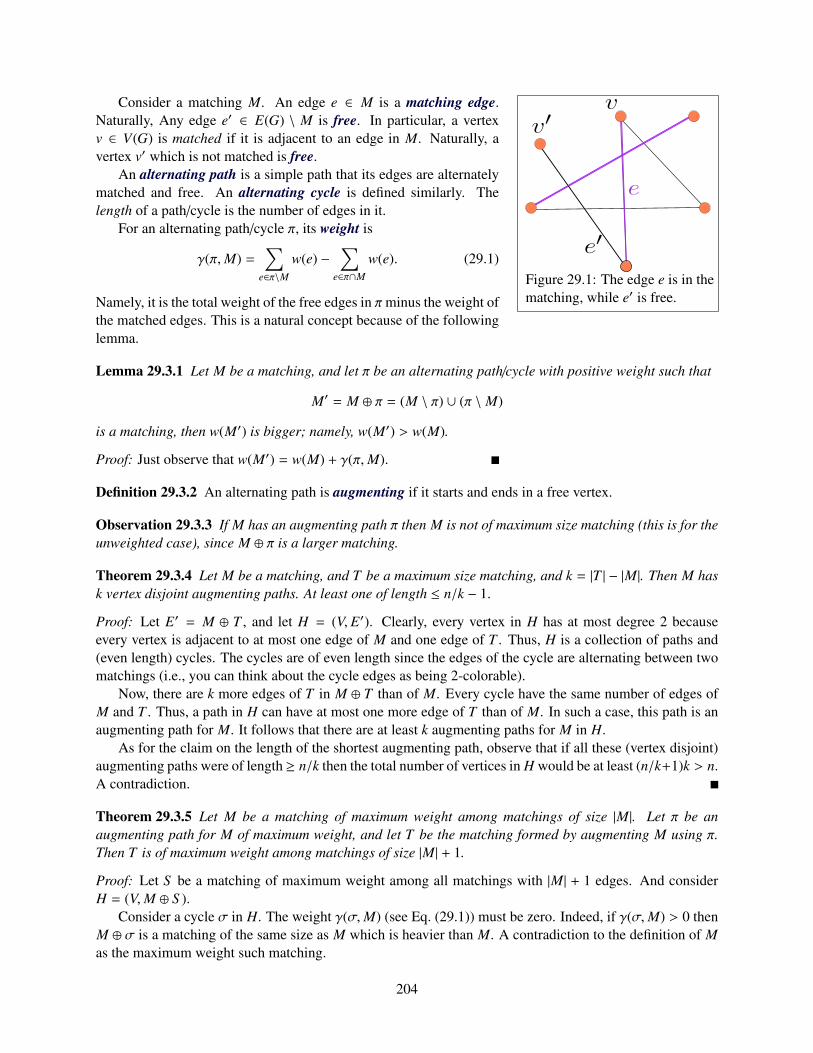
e

e′

vv′

Figure 29.1: The edge e is in thematching, while e′ is free.

Consider a matching M. An edge e ∈ M is a matching edge.Naturally, Any edge e′ ∈ E(G) \ M is free. In particular, a vertexv ∈ V(G) is matched if it is adjacent to an edge in M. Naturally, avertex v′ which is not matched is free.

An alternating path is a simple path that its edges are alternatelymatched and free. An alternating cycle is defined similarly. Thelength of a path/cycle is the number of edges in it.

For an alternating path/cycle π, its weight is

γ(π,M) =∑

e∈π\M

w(e) −∑

e∈π∩M

w(e). (29.1)

Namely, it is the total weight of the free edges in πminus the weight ofthe matched edges. This is a natural concept because of the followinglemma.

Lemma 29.3.1 Let M be a matching, and let π be an alternating path/cycle with positive weight such that

M′ = M ⊕ π = (M \ π) ∪ (π \ M)

is a matching, then w(M′) is bigger; namely, w(M′) > w(M).

Proof: Just observe that w(M′) = w(M) + γ(π,M).

Definition 29.3.2 An alternating path is augmenting if it starts and ends in a free vertex.

Observation 29.3.3 If M has an augmenting path π then M is not of maximum size matching (this is for theunweighted case), since M ⊕ π is a larger matching.

Theorem 29.3.4 Let M be a matching, and T be a maximum size matching, and k = |T | − |M|. Then M hask vertex disjoint augmenting paths. At least one of length ≤ n/k − 1.

Proof: Let E′ = M ⊕ T , and let H = (V, E′). Clearly, every vertex in H has at most degree 2 becauseevery vertex is adjacent to at most one edge of M and one edge of T . Thus, H is a collection of paths and(even length) cycles. The cycles are of even length since the edges of the cycle are alternating between twomatchings (i.e., you can think about the cycle edges as being 2-colorable).

Now, there are k more edges of T in M ⊕ T than of M. Every cycle have the same number of edges ofM and T . Thus, a path in H can have at most one more edge of T than of M. In such a case, this path is anaugmenting path for M. It follows that there are at least k augmenting paths for M in H.

As for the claim on the length of the shortest augmenting path, observe that if all these (vertex disjoint)augmenting paths were of length ≥ n/k then the total number of vertices in H would be at least (n/k+1)k > n.A contradiction.

Theorem 29.3.5 Let M be a matching of maximum weight among matchings of size |M|. Let π be anaugmenting path for M of maximum weight, and let T be the matching formed by augmenting M using π.Then T is of maximum weight among matchings of size |M| + 1.

Proof: Let S be a matching of maximum weight among all matchings with |M| + 1 edges. And considerH = (V,M ⊕ S ).

Consider a cycle σ in H. The weight γ(σ,M) (see Eq. (29.1)) must be zero. Indeed, if γ(σ,M) > 0 thenM ⊕ σ is a matching of the same size as M which is heavier than M. A contradiction to the definition of Mas the maximum weight such matching.

204

Similarly, if γ(σ,M) < 0 than γ(σ, S ) = −γ(σ,M) and as such S ⊕σ is heavier than S . A contradiction.By the same argumentation, if σ is a path of even length in the graph H then γ(σ,M) = 0 by the same

argumentation.Let US be all the odd length paths in H that have one edge more in S than in M, and similarly, let UM

be the odd length paths in H that have one edge more of M than an edge of S .We know that |US | − |UM | = 1 since S has one more edge than M. Now, consider a path π ∈ US and a

path π′ ∈ UM. It must be that γ(π,M)+γ(π′,M) = 0. Indeed, if γ(π,M)+γ(π′,M) > 0 then M⊕π⊕π′ wouldhave bigger weight than M while having the same number of edges. Similarly, if γ(π,M) + γ(π′,M) < 0(compared to M) then S ⊕π⊕π′ would have the same number of edges as S while being a heavier matching.A contradiction.

Thus, γ(π,M) + γ(π′,M) = 0. Thus, we can pair up the paths in US to paths in UM, and the total weightof such a pair is zero, by the above argumentation. There is only one path µ in US which is not paired, andit must be that γ(µ,M) = w(S ) − w(M) (since everything else in H has zero weight as we apply it to M toget S ).

This establishes the claim that we can augment M with a single path to get a maximum weight matchingof cardinality |M| + 1. Clearly, this path must be the heaviest augmenting path that exists for M. Otherwise,there would be a heavier augmenting path σ′ for M such that w(M ⊕ σ′) > w(S ). A contradiction to themaximality of S .

The above theorem imply that if we always augment along the maximum weight augmenting path, thanwe would get the maximum weight matching in the end.

29.4 Maximum Weight Matchings in A Bipartite Graph

Let G = (L∪R, E) be the given bipartite graph, with w : E → IR be the non-negative weight function. Givena matching M we define the graph GM to be the directed graph, where if rl ∈ M, l ∈ L and r ∈ R then we add(r → l) to E(GM) with weight α((r → l)) = w(rl) Similarly, if rl ∈ E \M then add the edge (l→ r) ∈ E(GM)to GM and set α((l→ r)) = −w(rl)

Namely, we direct all the matching edges from right to left, and assign them their weight, and we directall other edges from left to right, with their negated weight. Let GM denote the resulting graph.

An augmenting path π in G must have an odd number of edges. Since G is bipartite, π must have oneendpoint on the left side and one endpoint on the right side. Observe, that a path π in GM has weightα(π) = −γ(π,M).

Let UL be all the unmatched vertices in L and let UR be all the unmatched vertices in R.Thus, what we are looking for is a path π in GM starting UL going to UR with maximum weight γ(π),

namely with minimum weight α(π).

Lemma 29.4.1 If M is a maximum weight matching with k edges in G, than there is no negative cycle inGM where α(·) is the associated weight function.

Proof: Assume for the sake of contradiction that there is a cycle C, and observe that γ(C) = −α(C) > 0.Namely, M ⊕C is a new matching with bigger weight and the same number of edges. A contradiction to themaximality of M.

The algorithm. So, we now can find a maximum weight in the bipartite graph G as follows: Find amaximum weight matching M with k edges, compute the maximum weight augmenting path for M, applyit, and repeat till M is maximal.

Thus, we need to find a minimum weight path in GM between UL and UR (because we flip weights).This is just computing a shortest path in the graph GM which does not have negative cycles, and this can just

205

be done by using the Bellman-Ford algorithm. Indeed, collapse all the vertices of UL into a single vertex,and all the uncovered vertices of UR into a single vertex. Let HM be the resulting graph. Clearly, we arelooking for the shortest path between the two vertices corresponding to UL and UR in HM and since thisgraph has no negative cycles, this can be done using the Bellman-Ford algorithm, which takes O(nm) time.We conclude:

Lemma 29.4.2 Given a bipartite graph G and a maximum weight matching M of size k one can find amaximum weight augmenting path for G in O(nm) time, where n is the number of vertices of G and m is thenumber of edges.

We need to apply this algorithm n/2 times at most, as such, we get:

Theorem 29.4.3 Given a weight bipartite graph G, with n vertices and m edges, one can compute a maxi-mum weight matching in G in O(n2m) time.

29.4.1 Faster Algorithm

It turns out, in fact, that the graph here is very special, and one can use the Dijkstra algorithm. We omit anyfurther details, and just state the result. The interested student can figure out the details (warning: this is noteasy).

Theorem 29.4.4 Given a weight bipartite graph G, with n vertices and m edges, one can compute a maxi-mum weight matching in G in O(n(n log n + m)) time.

29.5 The Bellman-Ford Algorithm - A Quick Reminder

The Bellman-Ford algorithm computes the shortest path from a single source s in a graph G that has nonegative cycles to all the vertices in the graph. Here G has n vertices and m edges. The algorithm works byinitializing all distances to the source to be ∞ (formally, for all u ∈ V(G), we set d[u] ← ∞ and d[s] ← 0).Then, it n times scans all the edges, and for every edge (u→ v) ∈ E(G) it performs a Relax(u, v) operation.The relax operation checks if x = d[u] + w

((u→ v)

)< d[v], and if so, it updates d[v] to x, where d[u]

denotes the current distance from s to u. Since Relax(u, v) operation can be performed in constant time, andwe scan all the edges n times, it follows that the overall running time is O(mn).

We claim that in the end of the execution of the algorithm the shortest path length from s to u is d[u],for all u ∈ V(G). Indeed, every time we scan the edges, we set at least one vertex distance to its final value(which is its shortest path length). More formally, all vertices that their shortest path to s have i edges,are being set to their shortest path length in the ith iteration of the algorithm, as can be easily proved byinduction. This implies the claim.

Notice, that if we want to detect negative cycles, we can ran Bellman-Ford for an additional iteration.If the distances changes, we know that there is a negative cycle somewhere in the graph.

206

Chapter 30

Matchings II

30.1 Maximum Size Matching in a Non-Bipartite Graph

The results from the previous lecture suggests a natural algorithm for computing a maximum size (i.e.,matching with maximum number of edges in it) matching in a general (i.e., not necessarily bipartite) graph.Start from an empty matching M and repeatedly find an augmenting path from an unmatched vertex to anunmatched vertex. Here we are discussing the unweighted case.

Notations. Let T be a given tree. For two vertices x, y ∈ V(T), let τxy denote the path in T between x andy. For two paths π and π′ that share an endpoint, let π || π′ denotes the path resulting from concatenating πto π′. For a path π, let |π| denote the number of edges in π.

30.1.1 Finding an augmenting path

s

u v

Figure 30.1: A cy-cle in the alternatingBFS tree.

We are given a graph G and a matching M, and we would to compute a biggermatching in G. We will do it by computing an augmenting path for M.

We first observe that if G has any edge with both endpoints being free, wecan just add it to the current matching. Thus, in the following, we assume thatfor all edges, at least one of their endpoint is covered by the current matching M.Our task is to find an augmenting path in M.

We start by collapsing the unmatched vertices to a single vertex s, and let Hbe the resulting graph. Next, we compute an alternating BFS of H starting froms. Formally, we perform a BFS on H starting from s such that for the even levelsof the tree the algorithm is allowed to traverse only edges in the matching M,and in odd levels the algorithm traverses the unmatched edges. Let T denote theresulting tree.

An augmenting path in G corresponds to an odd cycle in H with passingthrough the vertex s.

Definition 30.1.1 An edge uv ∈ E(G) is a bridge if the the following conditionsare met: (i) u and v have the same depth in T, (ii) if the depth of u in T is eventhen uv is free (i.e., uv < M, and (iii) if the depth of u in T is odd then uv ∈ M.

Note, that given an edge uv we can check if it is a bridge in constant time after linear time preprocessingof T and G.

The following is an easy technical lemma.

207

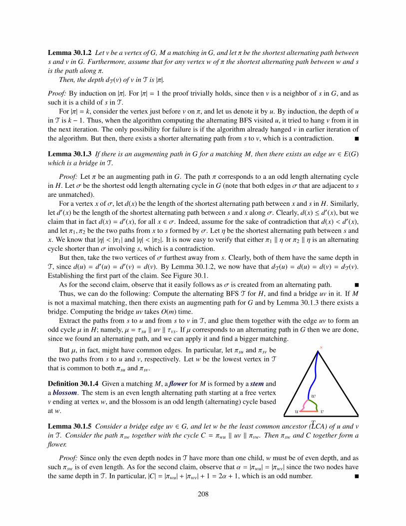
Lemma 30.1.2 Let v be a vertex of G, M a matching in G, and let π be the shortest alternating path betweens and v in G. Furthermore, assume that for any vertex w of π the shortest alternating path between w and sis the path along π.

Then, the depth dT(v) of v in T is |π|.

Proof: By induction on |π|. For |π| = 1 the proof trivially holds, since then v is a neighbor of s in G, and assuch it is a child of s in T.

For |π| = k, consider the vertex just before v on π, and let us denote it by u. By induction, the depth of uin T is k − 1. Thus, when the algorithm computing the alternating BFS visited u, it tried to hang v from it inthe next iteration. The only possibility for failure is if the algorithm already hanged v in earlier iteration ofthe algorithm. But then, there exists a shorter alternating path from s to v, which is a contradiction.

Lemma 30.1.3 If there is an augmenting path in G for a matching M, then there exists an edge uv ∈ E(G)which is a bridge in T.

Proof: Let π be an augmenting path in G. The path π corresponds to a an odd length alternating cyclein H. Let σ be the shortest odd length alternating cycle in G (note that both edges in σ that are adjacent to sare unmatched).

For a vertex x of σ, let d(x) be the length of the shortest alternating path between x and s in H. Similarly,let d′(x) be the length of the shortest alternating path between s and x along σ. Clearly, d(x) ≤ d′(x), but weclaim that in fact d(x) = d′(x), for all x ∈ σ. Indeed, assume for the sake of contradiction that d(x) < d′(x),and let π1, π2 be the two paths from x to s formed by σ. Let η be the shortest alternating path between s andx. We know that |η| < |π1| and |η| < |π2|. It is now easy to verify that either π1 || η or π2 || η is an alternatingcycle shorter than σ involving s, which is a contradiction.

But then, take the two vertices of σ furthest away from s. Clearly, both of them have the same depth inT, since d(u) = d′(u) = d′(v) = d(v). By Lemma 30.1.2, we now have that dT(u) = d(u) = d(v) = dT(v).Establishing the first part of the claim. See Figure 30.1.

As for the second claim, observe that it easily follows as σ is created from an alternating path.Thus, we can do the following: Compute the alternating BFS T for H, and find a bridge uv in it. If M

is not a maximal matching, then there exists an augmenting path for G and by Lemma 30.1.3 there exists abridge. Computing the bridge uv takes O(m) time.

Extract the paths from s to u and from s to v in T, and glue them together with the edge uv to form anodd cycle µ in H; namely, µ = τsu || uv || τvs. If µ corresponds to an alternating path in G then we are done,since we found an alternating path, and we can apply it and find a bigger matching.

s

w

u v

T

But µ, in fact, might have common edges. In particular, let πsu and πsv bethe two paths from s to u and v, respectively. Let w be the lowest vertex in T

that is common to both πsu and πsv.

Definition 30.1.4 Given a matching M, a flower for M is formed by a stem anda blossom. The stem is an even length alternating path starting at a free vertexv ending at vertex w, and the blossom is an odd length (alternating) cycle basedat w.

Lemma 30.1.5 Consider a bridge edge uv ∈ G, and let w be the least common ancestor (LCA) of u and vin T. Consider the path πsw together with the cycle C = πwu || uv || πvw. Then πsw and C together form aflower.

Proof: Since only the even depth nodes in T have more than one child, w must be of even depth, and assuch πsw is of even length. As for the second claim, observe that α = |πwu| = |πwv| since the two nodes havethe same depth in T. In particular, |C| = |πwu| + |πwv| + 1 = 2α + 1, which is an odd number.

208

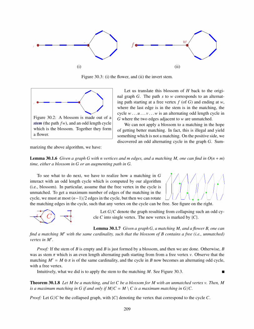
f

w

fw

(i) (ii)

Figure 30.3: (i) the flower, and (ii) the invert stem.

f

w

Figure 30.2: A blossom is made out of astem (the path f w), and an odd length cyclewhich is the blossom. Together they forma flower.

Let us translate this blossom of H back to the origi-nal graph G. The path s to w corresponds to an alternat-ing path starting at a free vertex f (of G) and ending at w,where the last edge is in the stem is in the matching, thecycle w . . . u . . . v . . .w is an alternating odd length cycle inG where the two edges adjacent to w are unmatched.

We can not apply a blossom to a matching in the hopeof getting better matching. In fact, this is illegal and yieldsomething which is not a matching. On the positive side, wediscovered an odd alternating cycle in the graph G. Sum-

marizing the above algorithm, we have:

Lemma 30.1.6 Given a graph G with n vertices and m edges, and a matching M, one can find in O(n + m)time, either a blossom in G or an augmenting path in G.

To see what to do next, we have to realize how a matching in Ginteract with an odd length cycle which is computed by our algorithm(i.e., blossom). In particular, assume that the free vertex in the cycle isunmatched. To get a maximum number of edges of the matching in thecycle, we must at most (n−1)/2 edges in the cycle, but then we can rotatethe matching edges in the cycle, such that any vertex on the cycle can be free. See figure on the right.

a

b

d

C a

b

d

C

Let G/C denote the graph resulting from collapsing such an odd cy-cle C into single vertex. The new vertex is marked by C.

Lemma 30.1.7 Given a graph G, a matching M, and a flower B, one canfind a matching M′ with the same cardinality, such that the blossom of B contains a free (i.e., unmatched)vertex in M′.

Proof: If the stem of B is empty and B is just formed by a blossom, and then we are done. Otherwise, Bwas as stem π which is an even length alternating path starting from from a free vertex v. Observe that thematching M′ = M ⊕ π is of the same cardinality, and the cycle in B now becomes an alternating odd cycle,with a free vertex.

Intuitively, what we did is to apply the stem to the matching M. See Figure 30.3.

Theorem 30.1.8 Let M be a matching, and let C be a blossom for M with an unmatched vertex v. Then, Mis a maximum matching in G if and only if M/C = M \C is a maximum matching in G/C.

Proof: Let G/C be the collapsed graph, with C denoting the vertex that correspond to the cycle C.

209

Note, that the collapsed vertex C in G/C is free. Thus, an augmenting path π in G/C either avoids thecollapsed vertex C altogether, or it starts or ends there. In any case, we can rotate the matching aroundC such that π would be an augmenting path in G. Thus, if M/C is not a maximum matching in G/C thenthere exists an augmenting path in G/C, which in turn is an augmenting path in G, and as such M is not amaximum matching in G.

Similarly, if π is an augmenting path in G and it avoids C then it is also an augmenting path in G/C, andthen M/C is not a maximum matching in G/C.

Otherwise, since π starts and ends in two different free vertices and C has only one free vertex, it followsthat π has an endpoint outside C. Let v be this endpoint of π and let u be the first vertex of π that belongs toC. Let σ be the path π[v, u].

Let f be the free vertex of C. Note that f is unmatched. Now, if u = f we are done, since then π is anaugmenting path also in G/C. Note that if u is matched in C, as such, it must be that the last edge e in πis unmatched. Thus, rotate the matching M around C such that u becomes free. Clearly, then σ is now anaugmenting path in G (for the rotated matching) and also an augmenting path in G/C.

Corollary 30.1.9 Let M be a matching, and let C be an alternating odd length cycle with the unmatchedvertex being free. Then, there is an augmenting path in G if and only if there is an augmenting path in G/C.

30.1.2 The algorithm

Start from the empty matching M in the graph G.Now, repeatedly, try to enlarge the matching. First, check if you can find an edge with both endpoints

being free, and if so add it to the matching. Otherwise, compute the graph H (this is the graph whereall the free vertices are collapsed into a single vertex), and compute an alternating BFS tree in H. Fromthe alternating BFS, we can extract the shortest alternating cycle based in the root (by finding the highestbridge). If this alternating cycle corresponds to an alternating path in G then we are done, as we can justapply this alternating path to the matching M getting a bigger matching.

If this is a flower, with a stem ρ and a blossom C then apply the stem to M (i.e., compute the matchingM ⊕ ρ). Now, C is an odd cycle with the free vertex being unmatched. Compute recursively an augmentingpath π in G/C. By the above discussing, we can easily transform this into an augmenting path in G. Applythis augmenting path to M.

Thus, we succeeded in computing a matching with one edge more in it. Repeat till the process get stuck.Clearly, what we have is a maximum size matching.

30.1.2.1 Running time analysis

Every shrink cost us O(m + n) time. We need to perform O(n) recursive shrink operations till we find anaugmenting path, if such a path exists. Thus, finding an augmenting path takes O(n(m + n)) time. Finally,we have to repeat this O(n) times. Thus, overall, the running time of our algorithm is O(n2(m+ n)) = O(n4).

Theorem 30.1.10 Given a graph G with n vertices and m edges, computing a maximum size matching in Gcan be done in O

(n2m

)time.

30.2 Maximum Weight Matching in A Non-Bipartite Graph

This the hardest case and it is non-trivial to handle. There are known polynomial time algorithms, but Ifeel that they are too involved, and somewhat cryptic, and as such should not be presented in class. For theinterested student, a nice description of such an algorithm is presented in

210

Combinatorial Optimization - Polyhedral and efficiencyby Alexander SchrijverVol. A, 453–459.

The description above also follows loosely the same book.

211

212

Part XIII

Union Find

213

Chapter 31

Union Find

31.1 Union-Find

31.1.1 Requirements from thedata-structure

We want to maintain a collection of sets,under the the following operations.

(i) UF_MakeSet(x) - creates a set thatcontains the single element x.

(ii) UF_Find(x) - returns the set thatcontains x.

(iii) UF_Union(A,B) - returns the setwhich is the union of A and B.Namely A ∪ B. Namely, this oper-ation merges the two sets A and Band return the merged set.

Scene: It’s a fine sunny day in the forest, and a rabbit is sittingoutside his burrow, tippy-tapping on his typewriter.Along comes a fox, out for a walk.Fox: “What are you working on?”Rabbit: “My thesis.”Fox: “Hmmm. What’s it about?”Rabbit: “Oh, I’m writing about how rabbits eat foxes.”Fox: (incredulous pause) “That’s ridiculous! Any fool knowsthat rabbits don’t eat foxes.”Rabbit: “Sure they do, and I can prove it. Come with me.”They both disappear into the rabbit’s burrow. After a few min-utes, the rabbit returns, alone, to his typewriter and resumestyping.Scene inside the rabbit’s burrow: In one corner, there is a pileof fox bones. In another corner, a pile of wolf bones. On theother side of the room, a huge lion is belching and picking histeeth.(The End)Moral: It doesn’t matter what you choose for a thesis subject.It doesn’t matter what you use for data.What does matter is who you have for a thesis advisor.

– – Anonymous

31.1.2 Amortized analysis

We use a data-structure as a black-box inside an algorithm (for example Union-Find in Kruskal algorithmfor computing minimum spanning tee). So far, when we design a data-structure we cared about worst casetime for operation. Note however, that this is not necessarily the right measure. Indeed, we care about theoverall running time spend on doing operations in the data-structure, and less about its running time for asingle operation.

Formally, the amortized running-time of an operation is the average time it takes to perform an operation

on the data-structure. Formally, the amortized time of an operation isoverall running timenumber of operations

.

31.1.3 The data-structure

215

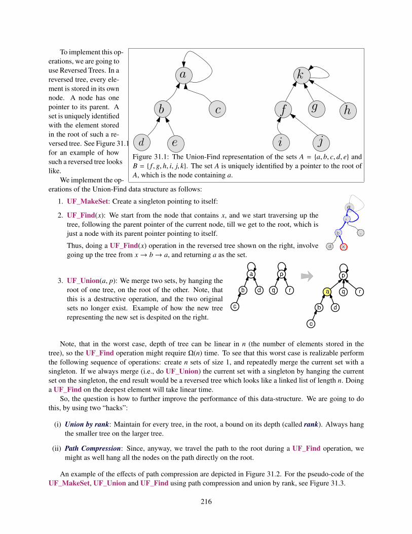
a

cb

ed

f g h

i j

k

Figure 31.1: The Union-Find representation of the sets A = a, b, c, d, e andB = f , g, h, i, j, k. The set A is uniquely identified by a pointer to the root ofA, which is the node containing a.

To implement this op-erations, we are going touse Reversed Trees. In areversed tree, every ele-ment is stored in its ownnode. A node has onepointer to its parent. Aset is uniquely identifiedwith the element storedin the root of such a re-versed tree. See Figure 31.1for an example of howsuch a reversed tree lookslike.

We implement the op-erations of the Union-Find data structure as follows:

a

1. UF_MakeSet: Create a singleton pointing to itself:

a

cb

xd

2. UF_Find(x): We start from the node that contains x, and we start traversing up thetree, following the parent pointer of the current node, till we get to the root, which isjust a node with its parent pointer pointing to itself.

Thus, doing a UF_Find(x) operation in the reversed tree shown on the right, involvegoing up the tree from x→ b→ a, and returning a as the set.

3. UF_Union(a, p): We merge two sets, by hanging theroot of one tree, on the root of the other. Note, thatthis is a destructive operation, and the two originalsets no longer exist. Example of how the new treerepresenting the new set is despited on the right.

Note, that in the worst case, depth of tree can be linear in n (the number of elements stored in thetree), so the UF_Find operation might require Ω(n) time. To see that this worst case is realizable performthe following sequence of operations: create n sets of size 1, and repeatedly merge the current set with asingleton. If we always merge (i.e., do UF_Union) the current set with a singleton by hanging the currentset on the singleton, the end result would be a reversed tree which looks like a linked list of length n. Doinga UF_Find on the deepest element will take linear time.

So, the question is how to further improve the performance of this data-structure. We are going to dothis, by using two “hacks”:

(i) Union by rank: Maintain for every tree, in the root, a bound on its depth (called rank). Always hangthe smaller tree on the larger tree.

(ii) Path Compression: Since, anyway, we travel the path to the root during a UF_Find operation, wemight as well hang all the nodes on the path directly on the root.

An example of the effects of path compression are depicted in Figure 31.2. For the pseudo-code of theUF_MakeSet, UF_Union and UF_Find using path compression and union by rank, see Figure 31.3.

216

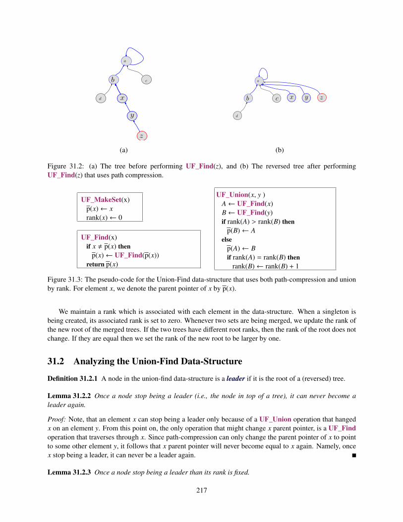
x

a

cb

d

y

z

x

a

cb

d

y z

(a) (b)

Figure 31.2: (a) The tree before performing UF_Find(z), and (b) The reversed tree after performingUF_Find(z) that uses path compression.

UF_MakeSet(x)p(x)← xrank(x)← 0

UF_Find(x)if x , p(x) then

p(x)← UF_Find(p(x))return p(x)

UF_Union(x, y )A← UF_Find(x)B← UF_Find(y)if rank(A) > rank(B) then

p(B)← Aelse

p(A)← Bif rank(A) = rank(B) then

rank(B)← rank(B) + 1

Figure 31.3: The pseudo-code for the Union-Find data-structure that uses both path-compression and unionby rank. For element x, we denote the parent pointer of x by p(x).

We maintain a rank which is associated with each element in the data-structure. When a singleton isbeing created, its associated rank is set to zero. Whenever two sets are being merged, we update the rank ofthe new root of the merged trees. If the two trees have different root ranks, then the rank of the root does notchange. If they are equal then we set the rank of the new root to be larger by one.

31.2 Analyzing the Union-Find Data-Structure

Definition 31.2.1 A node in the union-find data-structure is a leader if it is the root of a (reversed) tree.

Lemma 31.2.2 Once a node stop being a leader (i.e., the node in top of a tree), it can never become aleader again.

Proof: Note, that an element x can stop being a leader only because of a UF_Union operation that hangedx on an element y. From this point on, the only operation that might change x parent pointer, is a UF_Findoperation that traverses through x. Since path-compression can only change the parent pointer of x to pointto some other element y, it follows that x parent pointer will never become equal to x again. Namely, oncex stop being a leader, it can never be a leader again.

Lemma 31.2.3 Once a node stop being a leader than its rank is fixed.

217

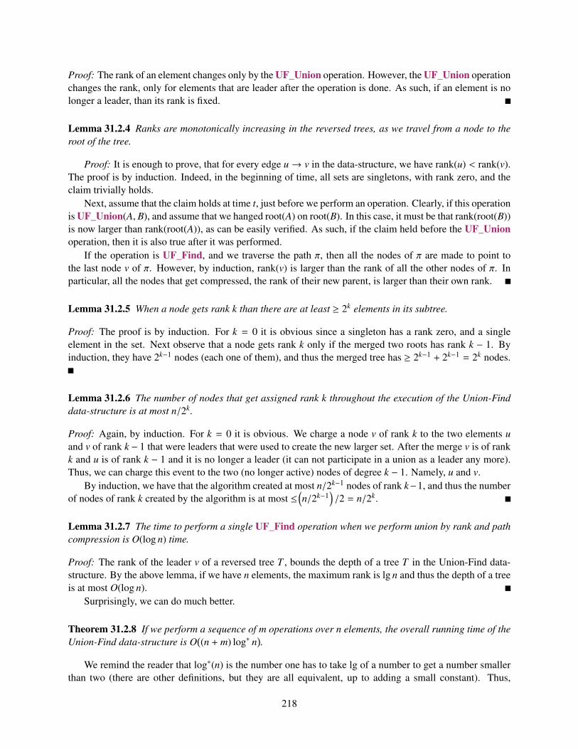
Proof: The rank of an element changes only by the UF_Union operation. However, the UF_Union operationchanges the rank, only for elements that are leader after the operation is done. As such, if an element is nolonger a leader, than its rank is fixed.

Lemma 31.2.4 Ranks are monotonically increasing in the reversed trees, as we travel from a node to theroot of the tree.

Proof: It is enough to prove, that for every edge u→ v in the data-structure, we have rank(u) < rank(v).The proof is by induction. Indeed, in the beginning of time, all sets are singletons, with rank zero, and theclaim trivially holds.

Next, assume that the claim holds at time t, just before we perform an operation. Clearly, if this operationis UF_Union(A, B), and assume that we hanged root(A) on root(B). In this case, it must be that rank(root(B))is now larger than rank(root(A)), as can be easily verified. As such, if the claim held before the UF_Unionoperation, then it is also true after it was performed.

If the operation is UF_Find, and we traverse the path π, then all the nodes of π are made to point tothe last node v of π. However, by induction, rank(v) is larger than the rank of all the other nodes of π. Inparticular, all the nodes that get compressed, the rank of their new parent, is larger than their own rank.

Lemma 31.2.5 When a node gets rank k than there are at least ≥ 2k elements in its subtree.

Proof: The proof is by induction. For k = 0 it is obvious since a singleton has a rank zero, and a singleelement in the set. Next observe that a node gets rank k only if the merged two roots has rank k − 1. Byinduction, they have 2k−1 nodes (each one of them), and thus the merged tree has ≥ 2k−1 + 2k−1 = 2k nodes.

Lemma 31.2.6 The number of nodes that get assigned rank k throughout the execution of the Union-Finddata-structure is at most n/2k.

Proof: Again, by induction. For k = 0 it is obvious. We charge a node v of rank k to the two elements uand v of rank k − 1 that were leaders that were used to create the new larger set. After the merge v is of rankk and u is of rank k − 1 and it is no longer a leader (it can not participate in a union as a leader any more).Thus, we can charge this event to the two (no longer active) nodes of degree k − 1. Namely, u and v.

By induction, we have that the algorithm created at most n/2k−1 nodes of rank k−1, and thus the numberof nodes of rank k created by the algorithm is at most ≤

(n/2k−1

)/2 = n/2k.

Lemma 31.2.7 The time to perform a single UF_Find operation when we perform union by rank and pathcompression is O(log n) time.

Proof: The rank of the leader v of a reversed tree T , bounds the depth of a tree T in the Union-Find data-structure. By the above lemma, if we have n elements, the maximum rank is lg n and thus the depth of a treeis at most O(log n).

Surprisingly, we can do much better.

Theorem 31.2.8 If we perform a sequence of m operations over n elements, the overall running time of theUnion-Find data-structure is O

((n + m) log∗ n

).

We remind the reader that log∗(n) is the number one has to take lg of a number to get a number smallerthan two (there are other definitions, but they are all equivalent, up to adding a small constant). Thus,

218

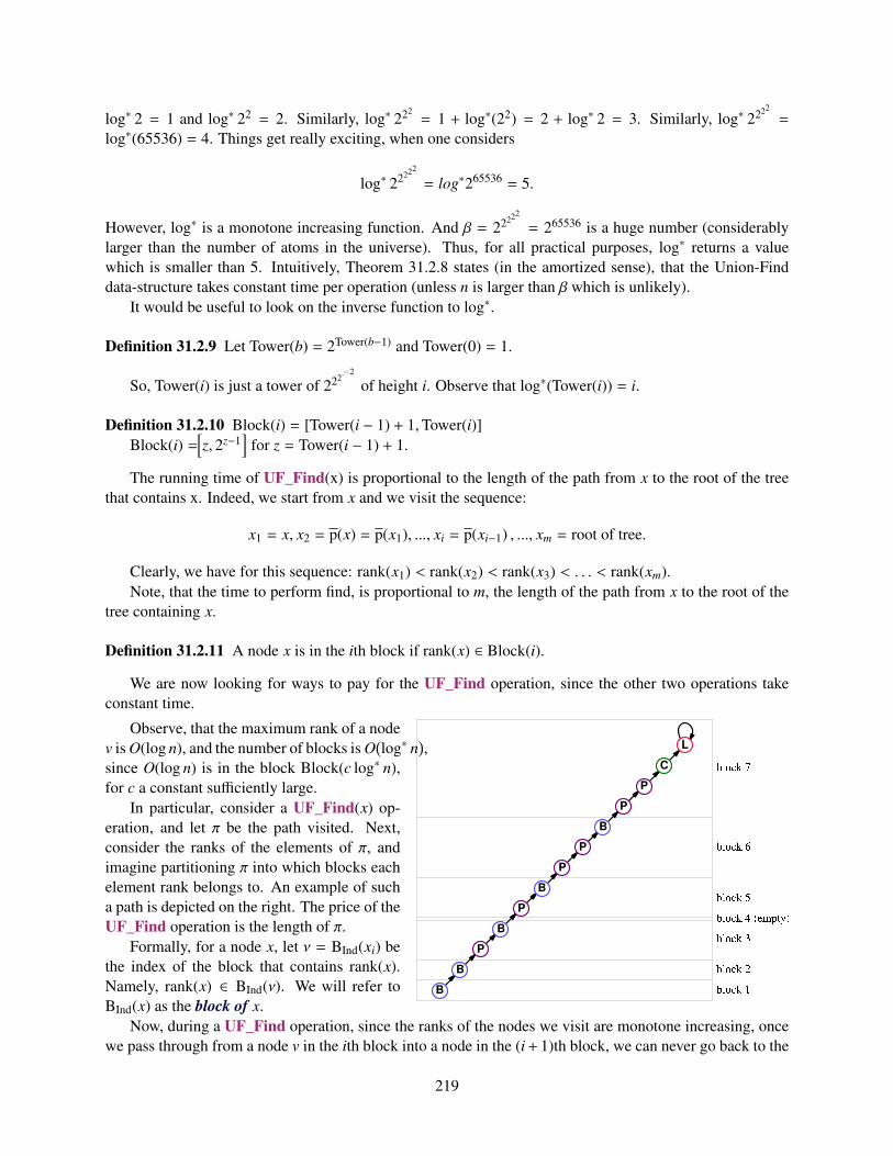
log∗ 2 = 1 and log∗ 22 = 2. Similarly, log∗ 222= 1 + log∗(22) = 2 + log∗ 2 = 3. Similarly, log∗ 2222

=

log∗(65536) = 4. Things get really exciting, when one considers

log∗ 22222

= log∗265536 = 5.

However, log∗ is a monotone increasing function. And β = 22222

= 265536 is a huge number (considerablylarger than the number of atoms in the universe). Thus, for all practical purposes, log∗ returns a valuewhich is smaller than 5. Intuitively, Theorem 31.2.8 states (in the amortized sense), that the Union-Finddata-structure takes constant time per operation (unless n is larger than β which is unlikely).

It would be useful to look on the inverse function to log∗.

Definition 31.2.9 Let Tower(b) = 2Tower(b−1) and Tower(0) = 1.

So, Tower(i) is just a tower of 222·· ·2

of height i. Observe that log∗(Tower(i)) = i.

Definition 31.2.10 Block(i) = [Tower(i − 1) + 1,Tower(i)]Block(i) =

[z, 2z−1

]for z = Tower(i − 1) + 1.

The running time of UF_Find(x) is proportional to the length of the path from x to the root of the treethat contains x. Indeed, we start from x and we visit the sequence:

x1 = x, x2 = p(x) = p(x1), ..., xi = p(xi−1) , ..., xm = root of tree.

Clearly, we have for this sequence: rank(x1) < rank(x2) < rank(x3) < . . . < rank(xm).Note, that the time to perform find, is proportional to m, the length of the path from x to the root of the

tree containing x.

Definition 31.2.11 A node x is in the ith block if rank(x) ∈ Block(i).

We are now looking for ways to pay for the UF_Find operation, since the other two operations takeconstant time.

Observe, that the maximum rank of a nodev is O(log n), and the number of blocks is O

(log∗ n

),

since O(log n) is in the block Block(c log∗ n),for c a constant sufficiently large.

In particular, consider a UF_Find(x) op-eration, and let π be the path visited. Next,consider the ranks of the elements of π, andimagine partitioning π into which blocks eachelement rank belongs to. An example of sucha path is depicted on the right. The price of theUF_Find operation is the length of π.

Formally, for a node x, let ν = BInd(xi) bethe index of the block that contains rank(x).Namely, rank(x) ∈ BInd(ν). We will refer toBInd(x) as the block of x.

Now, during a UF_Find operation, since the ranks of the nodes we visit are monotone increasing, oncewe pass through from a node v in the ith block into a node in the (i+ 1)th block, we can never go back to the

219

ith block (i.e., visit elements with rank in the ith block). As such, we can charge the visit to nodes in π thatare next to a element in a different block, to the number of blocks (which is O(log∗ n)).

Along the path π, we will refer to the parent point of an element x such that p(x) is in a different block,as a jump between blocks.

Lemma 31.2.12 During a single UF_Find(x) operation, the number of jumps between blocks along thesearch path is O

(log∗ n

).

Proof: Consider the search path π = x1, . . . , xm, and consider the list of numbers 0 ≤ BInd(x1) ≤ BInd(x2) ≤. . . ≤ BInd(xm). We have that BInd(xm) = O

(log∗ n

). As such, the number of elements x in π such that

BInd(x) , BInd(p(x)) is at most O(log∗ n).

Consider the case that x and p(x) are both the same block (i.e., BInd(x) = BInd(p(x)) and we perform afind operation that passes through x. Let rbef = rank(p(x)) before the UF_Find operation, and let raft berank(p(x)) after the UF_Find operation. Observe, that because of path compression, we have raft > rbef .Namely, when we jump inside a block, we do some work: we make the parent pointer of x jump forwardand the new parent has higher rank. We will charge such internal block jumps to this “progress”.

Definition 31.2.13 A jump during a find operation inside the ith block is called an internal jump.

Lemma 31.2.14 At most |Block(i)| ≤ Tower(i) UF_Find operations can pass through an element x, whichis in the ith block (i.e., BInd(x) = i) before p(x) is no longer in the ith block. That is BInd(p(x)) > i.

Proof: Indeed, by the above discussion, the parent of x increases its rank every-time an internal jumpgoes through x. Since there at most |Block(i)| different values in the ith block, the claim follows. Theinequality |Block(i)| ≤ Tower(i) holds by definition, see Definition 31.2.10.

Lemma 31.2.15 There are at most n/Tower(i) nodes that have ranks in the ith block throughout the algo-rithm execution.

Proof: By Lemma 31.2.6, we have that the number of elements with rank in the ith block is at most

∑k∈Block(i)

n2k =

Tower(i)∑k=Tower(i−1)+1

n2k = n ·

Tower(i)∑k=Tower(i−1)+1

12k ≤

n2Tower(i−1) =

nTower(i)

.

Lemma 31.2.16 The number of internal jumps performed, inside the ith block, during the lifetime of theunion-find data-structure is O(n).

Proof: An element x in the ith block, can have at most |Block(i)| internal jumps, before all jumps through xare jumps between blocks, by Lemma 31.2.14. There are at most n/Tower(i) elements with ranks in the ithblock, throughout the algorithm execution, by Lemma 31.2.15. Thus, the total number of internal jumps is

|Block(i)| ·n

Tower(i)≤ Tower(i) ·

nTower(i)

= n.

We are now ready for the last step.

Lemma 31.2.17 The number of internal jumps performed by the Union-Find data-structure overall isO(n log∗ n

).

220

Proof: Every internal jump can be associated with the block it is being performed in. Every block contributesO(n) internal jumps throughout the execution of the union-find data-structures, by Lemma 31.2.16. Thereare O(log∗ n) blocks. As such there are at most O(n log∗ n) internal jumps.

Lemma 31.2.18 The overall time spent on m UF_Find operations, throughout the lifetime of a union-finddata-structure defined over n elements, is O

((m + n) log∗ n

).

Theorem 31.2.8 now follows readily from the above discussion.

221

222

Part XIV

Exercises

223

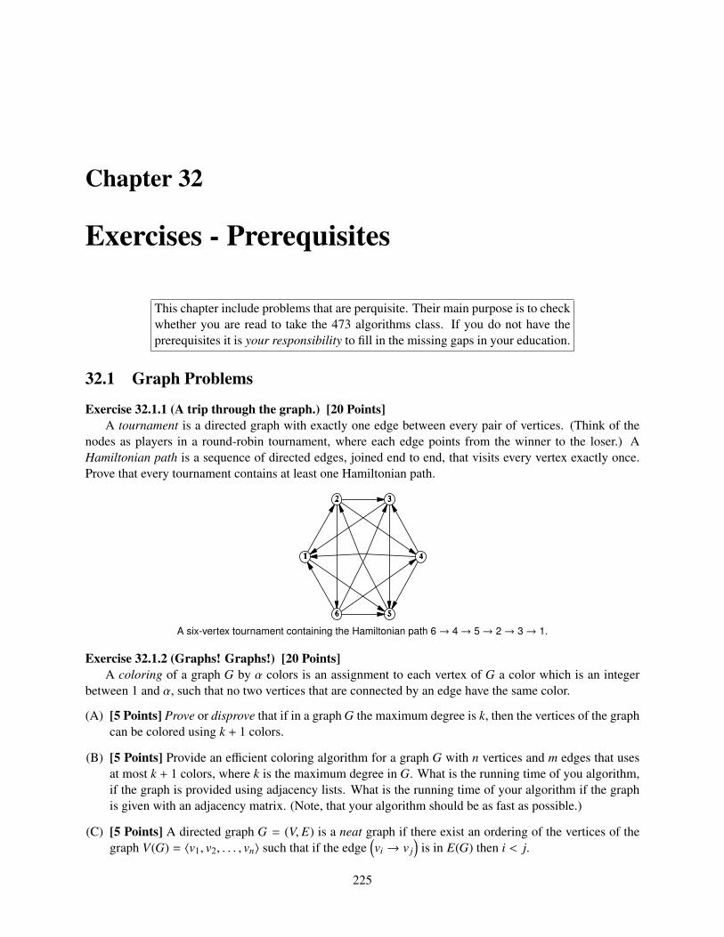
Chapter 32

Exercises - Prerequisites

This chapter include problems that are perquisite. Their main purpose is to checkwhether you are read to take the 473 algorithms class. If you do not have theprerequisites it is your responsibility to fill in the missing gaps in your education.

32.1 Graph Problems

Exercise 32.1.1 (A trip through the graph.) [20 Points]A tournament is a directed graph with exactly one edge between every pair of vertices. (Think of the

nodes as players in a round-robin tournament, where each edge points from the winner to the loser.) AHamiltonian path is a sequence of directed edges, joined end to end, that visits every vertex exactly once.Prove that every tournament contains at least one Hamiltonian path.

1

2

3

4

5

6

A six-vertex tournament containing the Hamiltonian path 6→ 4→ 5→ 2→ 3→ 1.

Exercise 32.1.2 (Graphs! Graphs!) [20 Points]A coloring of a graph G by α colors is an assignment to each vertex of G a color which is an integer

between 1 and α, such that no two vertices that are connected by an edge have the same color.

(A) [5 Points] Prove or disprove that if in a graph G the maximum degree is k, then the vertices of the graphcan be colored using k + 1 colors.

(B) [5 Points] Provide an efficient coloring algorithm for a graph G with n vertices and m edges that usesat most k + 1 colors, where k is the maximum degree in G. What is the running time of you algorithm,if the graph is provided using adjacency lists. What is the running time of your algorithm if the graphis given with an adjacency matrix. (Note, that your algorithm should be as fast as possible.)

(C) [5 Points] A directed graph G = (V, E) is a neat graph if there exist an ordering of the vertices of thegraph V(G) = 〈v1, v2, . . . , vn〉 such that if the edge

(vi → v j

)is in E(G) then i < j.

225

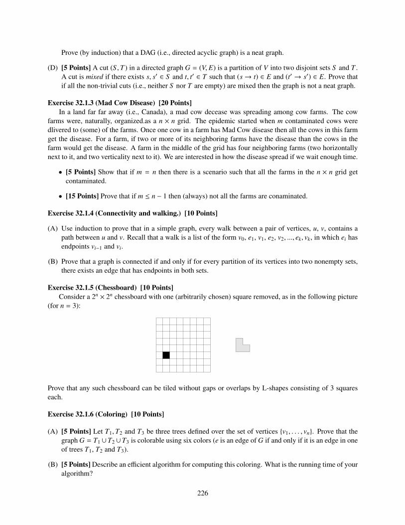
Prove (by induction) that a DAG (i.e., directed acyclic graph) is a neat graph.

(D) [5 Points] A cut (S ,T ) in a directed graph G = (V, E) is a partition of V into two disjoint sets S and T .A cut is mixed if there exists s, s′ ∈ S and t, t′ ∈ T such that (s→ t) ∈ E and (t′ → s′) ∈ E. Prove thatif all the non-trivial cuts (i.e., neither S nor T are empty) are mixed then the graph is not a neat graph.

Exercise 32.1.3 (Mad Cow Disease) [20 Points]In a land far far away (i.e., Canada), a mad cow decease was spreading among cow farms. The cow

farms were, naturally, organized.as a n × n grid. The epidemic started when m contaminated cows weredlivered to (some) of the farms. Once one cow in a farm has Mad Cow disease then all the cows in this farmget the disease. For a farm, if two or more of its neighboring farms have the disease than the cows in thefarm would get the disease. A farm in the middle of the grid has four neighboring farms (two horizontallynext to it, and two verticality next to it). We are interested in how the disease spread if we wait enough time.

• [5 Points] Show that if m = n then there is a scenario such that all the farms in the n × n grid getcontaminated.

• [15 Points] Prove that if m ≤ n − 1 then (always) not all the farms are conaminated.

Exercise 32.1.4 (Connectivity and walking.) [10 Points]

(A) Use induction to prove that in a simple graph, every walk between a pair of vertices, u, v, contains apath between u and v. Recall that a walk is a list of the form v0, e1, v1, e2, v2, ..., ek, vk, in which ei hasendpoints vi−1 and vi.

(B) Prove that a graph is connected if and only if for every partition of its vertices into two nonempty sets,there exists an edge that has endpoints in both sets.

Exercise 32.1.5 (Chessboard) [10 Points]Consider a 2n × 2n chessboard with one (arbitrarily chosen) square removed, as in the following picture

(for n = 3):

Prove that any such chessboard can be tiled without gaps or overlaps by L-shapes consisting of 3 squareseach.

Exercise 32.1.6 (Coloring) [10 Points]

(A) [5 Points] Let T1,T2 and T3 be three trees defined over the set of vertices v1, . . . , vn. Prove that thegraph G = T1 ∪T2 ∪T3 is colorable using six colors (e is an edge of G if and only if it is an edge in oneof trees T1, T2 and T3).

(B) [5 Points] Describe an efficient algorithm for computing this coloring. What is the running time of youralgorithm?

226

Exercise 32.1.7 (Binary trees and codes.) Professor George O’Jungle has a favorite 26-node binary tree,whose nodes are labeled by letters of the alphabet. The preorder and postorder sequences of nodes are asfollows:

preorder: M N H C R S K W T G D X I Y A J P O E Z V B U L Q Fpostorder: C W T K S G R H D N A O E P J Y Z I B Q L F U V X M

Draw Professor O’Jungle’s binary tree, and give the in-order sequence of nodes.

32.2 Recurrences

Exercise 32.2.1 (Recurrences.) [20 Points]Solve the following recurrences. State tight asymptotic bounds for each function in the form Θ( f (n))

for some recognizable function f (n). You do not need to turn in proofs (in fact, please don’t turn in proofs),but you should do them anyway just for practice. Assume reasonable but nontrivial base cases if none aresupplied. More exact solutions are better.

(A) [2 Points] A(n) = A(√

n/3 +⌊log n

⌋)+ n

(B) [2 Points] B(n) = min0<k<n

(3 + B(k) + B(n − k)

).

(C) [2 Points] C(n) = 3C(dn/2e − 5) + n/ log n

(D) [2 Points] D(n) = nn−3 D(n − 1) + 1

(E) [2 Points] E(n) = E(b3n/4c) +√

n

(F) [2 Points] F(n) = F(⌊log n

⌋) + log n (Hard)

(G) [2 Points] G(n) = n +⌊√

n⌋·G(

⌊√n⌋)

(H) [2 Points] H(n) = log(H(n − 1)) + 1

(I) [2 Points] I(n) = 5I(⌊√

n⌋)+ 1

(J) [2 Points] J(n) = 3J(n/4) + 1

Exercise 32.2.2 (Recurrences II) [20 Points]Solve the following recurrences. State tight asymptotic bounds for each function in the form Θ( f (n))

for some recognizable function f (n). You do not need to turn in proofs (in fact, please don’t turn in proofs),but you should do them anyway just for practice. Assume reasonable but nontrivial base cases if none aresupplied. More exact solutions are better.

(A) [1 Points] A(n) = A(n/3 + 5 +

⌊log n

⌋)+ n log log n

(B) [1 Points] B(n) = min0<k<n

(3 + B(k) + B(n − k)

).

(C) [1 Points] C(n) = 3C(dn/2e − 5) + n/ log n

(D) [1 Points] D(n) = nn−5 D(n − 1) + 1

(E) [1 Points] E(n) = E(b3n/4c) + 1/√

n

227

(F) [1 Points] F(n) = F(⌊log2 n

⌋) + log n (Hard)

(G) [1 Points] G(n) = n + 7√

n ·G(⌊√

n⌋)

(H) [1 Points] H(n) = log2(H(n − 1)) + 1

(I) [1 Points] I(n) = I(⌊

n1/4⌋)+ 1

(J) [1 Points] J(n) = J(n −

⌊n/ log n

⌋)+ 1

Exercise 32.2.3 (Recurrences III) [20 Points]Solve the following recurrences. State tight asymptotic bounds for each function in the form Θ( f (n))

for some recognizable function f (n). You do not need to turn in proofs (in fact, please don’t turn in proofs),but you should do them anyway just for practice. Assume reasonable but nontrivial base cases if none aresupplied.

(A) A(n) = A(n/2) + n

(B) B(n) = 2B(n/2) + n

(C) C(n) = n + 12(C(n − 1) +C(3n/4)

)(D) D(n) = max

n/3<k<2n/3

(D(k) + D(n − k) + n

)(Hard)

(E) E(n) = 2E(n/2) + n/ lg n (Hard)

(F) F(n) = F(n−1)F(n−2) , where F(1) = 1 and F(2) = 2. (Hard)

(G) G(n) = G(n/2) +G(n/4) +G(n/6) +G(n/12) + n [Hint: 12 +

14 +

16 +

112 = 1.] (Hard)

(H) H(n) = n +√

n · H(√

n) (Hard)

(I) I(n) = (n − 1)(I(n − 1) + I(n − 2)), where F(0) = F(1) = 1 (Hard)

(J) J(n) = 8J(n − 1) − 15J(n − 2) + 1

Exercise 32.2.4 (Evaluate summations.) [10 Points] Evaluate the following summations; simplify youranswers as much as possible. Significant partial credit will be given for answers in the form Θ( f (n)) forsome recognizable function f (n).

(A) [2 Points]n∑

i=1

i∑j=1

i∑k= j

1i

(Hard)

(B) [2 Points]n∑

i=1

i∑j=1

i∑k= j

1j

(C) [2 Points]n∑

i=1

i∑j=1

i∑k= j

1k

228

(D) [2 Points]n∑

i=1

i∑j=1

j∑k=1

1k

(E) [2 Points]n∑

i=1

i∑j=1

j∑k=1

1j · k

Exercise 32.2.5 (Simplify binary formulas.) This problem asks you to simplify some recursively definedboolean formulas as much as possible. In each case, prove that your answer is correct. Each proof can bejust a few sentences long, but it must be a proof.

(A) Suppose α0 = p, α1 = q, and αn = (αn−2 ∧ αn−1) for all n ≥ 2. Simplify αn as much as possible. [Hint:What is α5?]

(B) Suppose β0 = p, β1 = q, and βn = (βn−2 ⇔ βn−1) for all n ≥ 2. Simplify βn as much as possible. [Hint:What is β5?]

(C) Suppose γ0 = p, γ1 = q, and γn = (γn−2 ⇒ γn−1) for all n ≥ 2. Simplify γn as much as possible. [Hint:What is γ5?]

(D) Suppose δ0 = p, δ1 = q, and δn = (δn−2 1 δn−1) for all n ≥ 2, where 1 is some boolean function withtwo arguments. Find a boolean function 1 such that δn = δm if and only if n − m is a multiple of 4.[Hint: There is only one such function.]

32.3 Counting

Exercise 32.3.1 (Counting dominos) (A) A domino is a 2×1 or 1×2 rectangle. How many different waysare there to completely fill a 2 × n rectangle with n dominos? Set up a recurrence relation and give anexact closed-form solution.

(B) A slab is a three-dimensional box with dimensions 1 × 2 × 2, 2 × 1 × 2, or 2 × 2 × 1. How manydifferent ways are there to fill a 2 × 2 × n box with n slabs? Set up a recurrence relation and give anexact closed-form solution.

A 2 × 10 rectangle filled with ten dominos, and a 2 × 2 × 10 box filled with ten slabs.

32.4 O notation and friends

Exercise 32.4.1 (Sorting functions) [20 Points]Sort the following 25 functions from asymptotically smallest to asymptotically largest, indicating ties if

there are any. You do not need to turn in proofs (in fact, please don’t turn in proofs), but you should do them

229

anyway just for practice.

n4.5 − (n − 1)4.5 n n2.1 lg∗(n/8) 1 + lg lg lg n

cos n + 2 lg(lg∗ n) (lg n)! (lg∗ n)lg n n5

lg∗ 222n

2lg n √ne ∑n

i=1 i∑n

i=1 i2

n7/(2n) n3/(2 lg n) 12 +⌊lg lg(n)

⌋(lg(2 + n))lg n

(1 + 1

154

)15n

n1/ lg lg n nlg lg n lg(201) n n1/125 n(lg n)4

To simplify notation, write f (n) g(n) to mean f (n) = o(g(n)) and f (n) ≡ g(n) to mean f (n) = Θ(g(n)). Forexample, the functions n2, n,

(n2

), n3 could be sorted either as n n2 ≡

(n2

) n3 or as n

(n2

)≡ n2 n3.

[Hint: When considering two functions f (·) and g(·) it is sometime useful to consider the functions ln f (·)and ln g(·).]

Exercise 32.4.2 (Sorting functions II) [20 Points]Sort the following 25 functions from asymptotically smallest to asymptotically largest, indicating ties if

there are any. You do not need to turn in proofs (in fact, please don’t turn in proofs), but you should do themanyway just for practice.

n5.5 − (n − 1)5.5 n n2.2 lg∗(n/7) 1 + lg lg n

cos n + 2 lg(lg∗ n) lg(n!) (lg∗ n)lg n n4

lg∗ 22n2lg∗ n e

√n ∑n

i=11i

∑ni=1

1i2

n3/(2n) n3/(2 lg n) ⌊lg lg(n!)

⌋(lg(7 + n))lg n

(1 + 1

154

)154n

n1/ lg lg n nlg lg n lg(200) n n1/1234 n(lg n)3

To simplify notation, write f (n) g(n) to mean f (n) = o(g(n)) and f (n) ≡ g(n) to mean f (n) = Θ(g(n)). Forexample, the functions n2, n,

(n2

), n3 could be sorted either as n n2 ≡

(n2

) n3 or as n

(n2

)≡ n2 n3.

Exercise 32.4.3 (O notation revisited.) [10 Points]

(A) Let fi(n) be a sequence of functions, such that for every i, fi(n) = o(√

n) (namely, limn→∞fi(n)√

n= 0).

Let g(n) =∑n

i=1 fi(n). Prove or disprove: g(n) = o(n3/2).

(B) If f1(n) = O(g1(n)) and f2(n) = O(g2(n)). Prove or disprove:

• f1(n) + f2(n) = O(g1(n) + g2(n))• f1(n) ∗ f2(n) = O(g1(n) ∗ g2(n))• f1(n) f2(n) = O(g1(n)g2(n))

Exercise 32.4.4 (Some proofs required.) (A) Prove that 2dlg ne+blg nc = Θ(n2).

(B) Prove or disprove: 2blg nc = Θ(2dlg ne).

(C) Prove or disprove: 22blg lg nc= Θ

(22dlg lg ne).

(D) Prove or disprove: If f (n) = O(g(n)), then log( f (n)) = O(log(g(n))).

(E) Prove or disprove: If f (n) = O(g(n)), then 2 f (n) = O(2g(n)).

(Hard)

(F) Prove that logk n = o(n1/k) for any positive integer k.

230

32.5 Probability

Exercise 32.5.1 (Balls and boxes.) [20 Points] There are n balls (numbered from 1 to n) and n boxes (num-bered from 1 to n). We put each ball in a randomly selected box.

(A) [4 Points] A box may contain more than one ball. Suppose X is the number on the box that has thesmallest number among all nonempty boxes. What is the expectation of X?

(B) [4 Points] What is the expected number of bins that have exactly one ball in them? (Hint: Compute theprobability of a specific bin to contain exactly one ball and then use some properties of expectation.)

(C) [8 Points] We put the balls into the boxes in such a way that there is exactly one ball in each box. If thenumber written on a ball is the same as the number written on the box containing the ball, we say thereis a match. What is the expected number of matches?

(D) [4 Points] What is the probability that there are exactly k matches? (1 ≤ k < n)

[Hint: If you have to appeal to “intuition” or “common sense”, your answers are probably wrong!]

Exercise 32.5.2 (Idiotic Sort) [20 Points]There is an array A with n unsorted distinct numbers in it. IS(A) sorts the array using an iterative

algorithm. In each iteration, it picks randomly (and uniformly) two indices i, j in the ranges 1, . . . , n. Next,if A[min(i, j)] > A[max(i, j)] it swaps A[i] and A[ j]. The algorithm magically stop once the array is sorted.

(A) [5 Points] Prove that after (at most) n! swaps performed by the algorithm, the array A is sorted.

(B) [5 Points] Prove that after at most (say) 6n3 swaps performed by the algorithm, the array A is sorted.(There might be an easy solution, but I don’t see it.)

(C) [5 Points] Prove that if A is not sorted, than the probability for a swap in the next iteration is at least≥ 2/n2.

(D) [5 Points] Prove that if A is not sorted, then the expected number of iterations till the next swap is≤ n2/2. [Hint: use geometric random variable.]

(E) [5 Points] Prove that the expected number of iterations performed by the algorithm is O(n5). [Hint:Use linearity of expectation.]

Exercise 32.5.3 (Random walk.) [10 Points]A random walk is a walk on a graph G, generated by starting from a vertex v0 = v ∈ V(G), and in the

i-th stage, for i > 0, randomly selecting one of the neighbors of vi−1 and setting vi to be this vertex. A walkv0, v1, . . . , vm is of length m.

(A) For a vertex u ∈ V(G), let Pu(m, v) be the probability that a random walk of length m, starting from u,visits v (i.e., vi = v for some i).

Prove that a graph G with n vertices is connected, if and only if, for any two vertices u, v ∈ V(G), wehave Pu(n − 1, v) > 0.

(B) Prove that a graph G with n vertices is connected if and only if for any pair of vertices u, v ∈ V(G), wehave limm→∞ Pu(m, v) = 1.

231

Exercise 32.5.4 (Random Elections.) [10 Points]You are in a shop trying to buy green tea. There n different types of green tea that you are considering:

T1, . . . ,Tn. You have a coin, and you decide to randomly choose one of them using random coin flips.Because of the different prices of the different teas, you decide that you want to choose the ith tea withprobability pi (of course,

∑ni=1 pi = 1).

Describe an algorithm that chooses a tea according to this distribution, using only coin flips. Computethe expected number of coin flips your algorithm uses. (Your algorithm should minimize the number of coinflips it uses, since if you flip coins too many times in the shop, you might be arrested.)

Exercise 32.5.5 (Runs?) [10 Points]We toss a fair coin n times. What is the expected number of “runs”? Runs are consecutive tosses with

the same result. For example, the toss sequence HHHTTHTH has 5 runs.

Exercise 32.5.6 (A card game.) Penn and Teller have a special deck of fifty-two cards, with no face cardsand nothing but clubs—the ace, 2, 3, 4, 5, 6, 7, 8, 9, 10, 11, 12, . . . , 52 of clubs. (They’re big cards.) Pennshuffles the deck until each of the 52! possible orderings of the cards is equally likely. He then takes cardsone at a time from the top of the deck and gives them to Teller, stopping as soon as he gives Teller the fiveof clubs.

(A) On average, how many cards does Penn give Teller?

(B) On average, what is the smallest-numbered card that Penn gives Teller? (Hard)

(C) On average, what is the largest-numbered card that Penn gives Teller?

[Hint: Solve for an n-card deck and then set n = 52.] In each case, give exact answers and prove that theyare correct. If you have to appeal to “intuition” or “common sense”, your answers are probably wrong!

Exercise 32.5.7 (Alice and Bob) Alice and Bob each have a fair n-sided die. Alice rolls her die once. Bobthen repeatedly throws his die until he rolls a number at least as big as the number Alice rolled. Each timeBob rolls, he pays Alice $1. (For example, if Alice rolls a 5, and Bob rolls a 4, then a 3, then a 1, then a5, the game ends and Alice gets $4. If Alice rolls a 1, then no matter what Bob rolls, the game will endimmediately, and Alice will get $1.)

Exactly how much money does Alice expect to win at this game? Prove that your answer is correct. Ifyou have to appeal to ‘intuition’ or ‘common sense’, your answer is probably wrong!

32.6 Basic data-structures and algorithms

Exercise 32.6.1 (Storing temperatures.) [10 Points]Describe a data structure that supports storing temperatures. The operations on the data structure are as

follows:

Insert(t, d) — Insert the temperature t that was measured on date d. Each temperature is a real numberbetween −100 and 150. For example, insert(22, ”1/20/03”).

Average(d1, d2) report what is the average of all temperatures that were measured between date d1 anddate d2.

Each operation should take time O(log n), where n is the number of dates stored in the data structure. Youcan assume that a date is just an integer which specifies the number of days since the first of January 1970.

232

Exercise 32.6.2 (Binary search tree modifications.) [10 Points]Suppose we have a binary search tree. You perform a long sequence of operations on the binary tree

(insertion, deletions, searches, etc), and the maximum depth of the tree during those operations is at most h.Modify the binary search tree T so that it supports the following operations. Implementing some of

those operations would require you to modify the information stored in each node of the tree, and the wayinsertions/deletions are being handled in the tree. For each of the following, describe separately the changesmade in detail, and the algorithms for answering those queries. (Note, that under the modified version of thebinary search tree, insertion and deletion should still take O(h) time, where h is the maximum height of thetree during all the execution of the algorithm.)

(A) [2 Points] Find the smallest element stored in T in O(h) time.

(B) [2 Points] Given a query k, find the k-th smallest element stored in T in O(h) time.

(C) [3 Points] Given a query [a, b], find the number of elements stored in T with their values being in therange [a, b], in O(h) time.

(D) [3 Points] Given a query [a, b], report (i.e., printout) all the elements stored in T in the range [a, b], inO(h + u) time, where u is the number of elements printed out.

Exercise 32.6.3 (Euclid revisited.) [10 Points]Prove that for any nonnegative parameters a and b, the following algorithms terminate and produce

identical output. Also, provide bounds on the running times of those algorithms. Can you imagine anyreason why WE would be preferable to FE?

SlowEuclid(a, b) :if b > a

return SE(b, a)else if b = 0

return aelse

return SE(b, a − b)

FastEuclid(a, b) :if b = 0

return aelse

return FE(b, a mod b)

WeirdEuclid(a, b) :if b = 0

return aif a = 0

return bif a is even and b is even

return 2∗WE(a/2, b/2)if a is even and b is odd

return WE(a/2, b)if a is odd and b is even

return WE(a, b/2)if b > a

return WE(b − a, a)else

return WE(a − b, b)

233

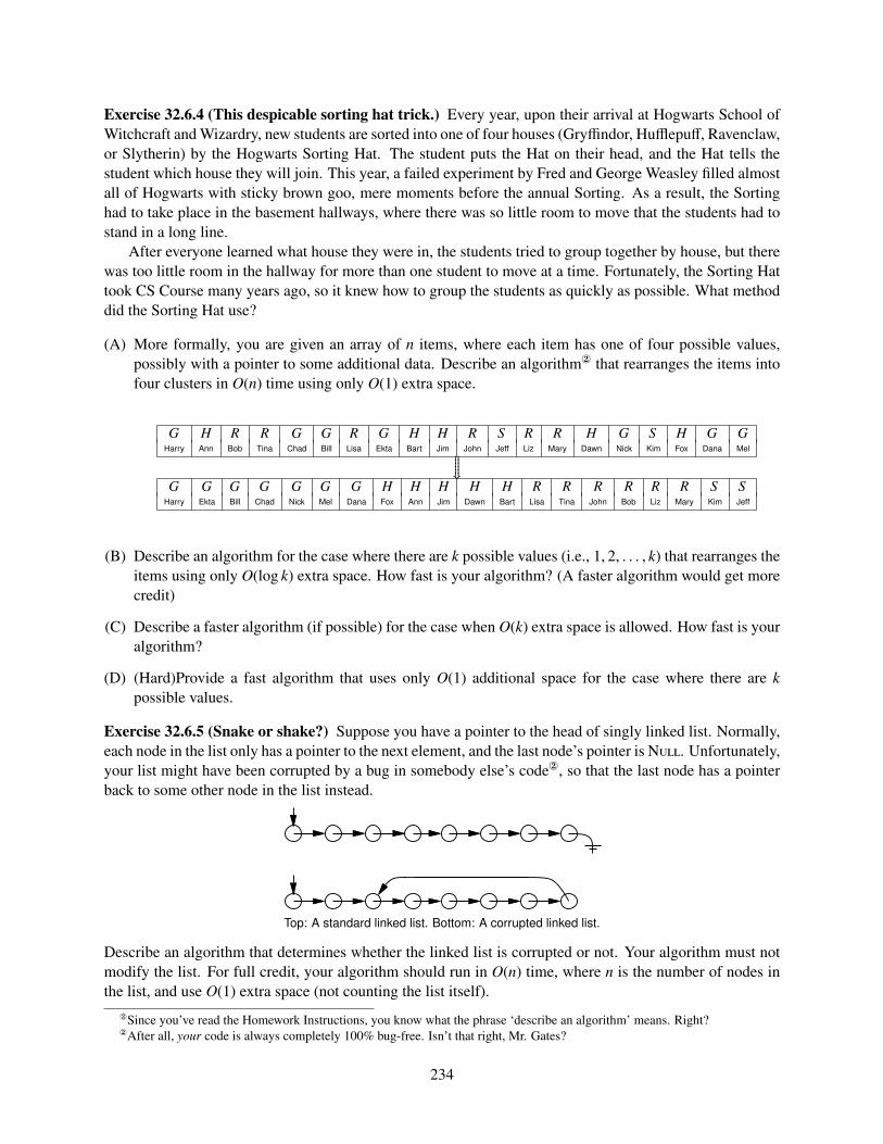
Exercise 32.6.4 (This despicable sorting hat trick.) Every year, upon their arrival at Hogwarts School ofWitchcraft and Wizardry, new students are sorted into one of four houses (Gryffindor, Hufflepuff, Ravenclaw,or Slytherin) by the Hogwarts Sorting Hat. The student puts the Hat on their head, and the Hat tells thestudent which house they will join. This year, a failed experiment by Fred and George Weasley filled almostall of Hogwarts with sticky brown goo, mere moments before the annual Sorting. As a result, the Sortinghad to take place in the basement hallways, where there was so little room to move that the students had tostand in a long line.

After everyone learned what house they were in, the students tried to group together by house, but therewas too little room in the hallway for more than one student to move at a time. Fortunately, the Sorting Hattook CS Course many years ago, so it knew how to group the students as quickly as possible. What methoddid the Sorting Hat use?

(A) More formally, you are given an array of n items, where each item has one of four possible values,possibly with a pointer to some additional data. Describe an algorithm that rearranges the items intofour clusters in O(n) time using only O(1) extra space.

G H R R G G R G H H R S R R H G S H G GHarry Ann Bob Tina Chad Bill Lisa Ekta Bart Jim John Jeff Liz Mary Dawn Nick Kim Fox Dana MelwwwwwG G G G G G G H H H H H R R R R R R S S

Harry Ekta Bill Chad Nick Mel Dana Fox Ann Jim Dawn Bart Lisa Tina John Bob Liz Mary Kim Jeff

(B) Describe an algorithm for the case where there are k possible values (i.e., 1, 2, . . . , k) that rearranges theitems using only O(log k) extra space. How fast is your algorithm? (A faster algorithm would get morecredit)

(C) Describe a faster algorithm (if possible) for the case when O(k) extra space is allowed. How fast is youralgorithm?

(D) (Hard)Provide a fast algorithm that uses only O(1) additional space for the case where there are kpossible values.

Exercise 32.6.5 (Snake or shake?) Suppose you have a pointer to the head of singly linked list. Normally,each node in the list only has a pointer to the next element, and the last node’s pointer is N. Unfortunately,your list might have been corrupted by a bug in somebody else’s code, so that the last node has a pointerback to some other node in the list instead.

Top: A standard linked list. Bottom: A corrupted linked list.

Describe an algorithm that determines whether the linked list is corrupted or not. Your algorithm must notmodify the list. For full credit, your algorithm should run in O(n) time, where n is the number of nodes inthe list, and use O(1) extra space (not counting the list itself).

Since you’ve read the Homework Instructions, you know what the phrase ‘describe an algorithm’ means. Right?After all, your code is always completely 100% bug-free. Isn’t that right, Mr. Gates?

234

32.7 General proof thingies

Exercise 32.7.1 (Cornification) [20 Points]Cornification - Conversion into, or formation of, horn; a becoming like horn. Source: Webster’s Revised

Unabridged Dictionary.During the sweetcorn festival in Urbana, you had been kidnapped by an extreme anti corn organization

called Al Corona. To punish you, they give you several sacks with a total of (n+1)n/2 cobs of corn in them,and an infinite supply of empty sacks. Next, they ask you to play the following game: At every point intime, you take a cob from every non-empty sack, and you put this set of cobs into a new sack. The gameterminates when you have n non-empty sacks, with the ith sack having i cobs in it, for i = 1, . . . , n.

For example, if we started with 1, 5 (i.e., one sack has 1 cob, the other 5), we would have the followingsequence of steps: 2, 4, 1, 2, 3 and the game ends.

(A) [5 Points] Prove that the game terminates if you start from a configuration where all the cobs are in asingle sack.

(B) [5 Points] Provide a bound, as tight as possible, on the number of steps in the game till it terminates inthe case where you start with a single sack.

(C) [5 Points] (hard) Prove that the game terminates if you start from an arbitrary configuration where thecobs might be in several sacks.

(D) [5 Points] Provide a bound, as tight as possible, on the number of steps in the game till it terminates inthe general case.

Exercise 32.7.2 (Fibonacci numbers.) Recall the standard recursive definition of the Fibonacci numbers:F0 = 0, F1 = 1, and Fn = Fn−1 + Fn−2 for all n ≥ 2. Prove the following identities for all positive integersn and m.

(A) Fn is even if and only if n is divisible by 3.

(B)∑n

i=0 Fi = Fn+2 − 1

(C) F2n − Fn+1Fn−1 = (−1)n+1 (Really Hard)

(D) If n is an integer multiple of m, then Fn is an integer multiple of Fm.

Exercise 32.7.3 (Some binomial identities.) (A) Prove the following identity by induction:(2nn

)=

n∑k=0

(nk

)(n

n − k

).

(B) Give a non-inductive combinatorial proof of the same identity, by showing that the two sides of theequation count exactly the same thing in two different ways. There is a correct one-sentence proof.

32.8 Miscellaneous

Exercise 32.8.1 (A walking ant.) (Hard)An ant is walking along a rubber band, starting at the left end.Once every second, the ant walks one inch to the right, and then you make the rubber band one inch longerby pulling on the right end. The rubber band stretches uniformly, so stretching the rubber band also pullsthe ant to the right. The initial length of the rubber band is n inches, so after t seconds, the rubber band isn + t inches long.

235

t=0

t=2

t=1

Every second, the ant walks an inch, and then the rubber band is stretched an inch longer.

(A) How far has the ant moved after t seconds, as a function of n and t? Set up a recurrence and (for fullcredit) give an exact closed-form solution. [Hint: What fraction of the rubber band’s length has the antwalked?]

(B) How long does it take the ant to get to the right end of the rubber band? For full credit, give an answerof the form f (n) + Θ(1) for some explicit function f (n).

236

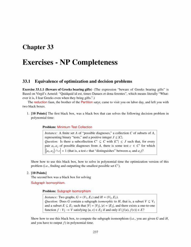
Chapter 33

Exercises - NP Completeness

33.1 Equivalence of optimization and decision problems

Exercise 33.1.1 (Beware of Greeks bearing gifts) (The expression “beware of Greeks bearing gifts” isBased on Virgil’s Aeneid: “Quidquid id est, timeo Danaos et dona ferentes”, which means literally “What-ever it is, I fear Greeks even when they bring gifts.”.)

The reduction faun, the brother of the Partition satyr, came to visit you on labor day, and left you withtwo black boxes.

1. [10 Points] The first black box, was a black box that can solves the following decision problem inpolynomial time:

Problem: Minimum Test Collection

Instance: A finite set A of “possible diagnoses,” a collection C of subsets of A,representing binary “tests,” and a positive integer J ≤ |C|.Question: Is there a subcollection C′ ⊆ C with |C′| ≤ J such that, for everypair ai, a j of possible diagnoses from A, there is some test c ∈ C′ for which∣∣∣∣ai, a j

∩ c

∣∣∣∣ = 1 (that is, a test c that “distinguishes” between ai and a j)?

Show how to use this black box, how to solve in polynomial time the optimization version of thisproblem (i.e., finding and outputting the smallest possible set C′).

2. [10 Points]The second box was a black box for solving

Subgraph Isomorphism.

Problem: Subgraph Isomorphism

Instance: Two graphs, G = (V1, E1) and H = (V2, E2).Question: Does G contain a subgraph isomorphic to H, that is, a subset V ⊆ V1and a subset E ⊆ E1 such that |V | = |V2|, |e| = |E2|, and there exists a one-to-onefunction f : V2 → V satisfying u, v ∈ E2 if and only if f (u), f (v) ∈ E?

Show how to use this black box, to compute the subgraph isomorphism (i.e., you are given G and H,and you have to output f ) in polynomial time.

237

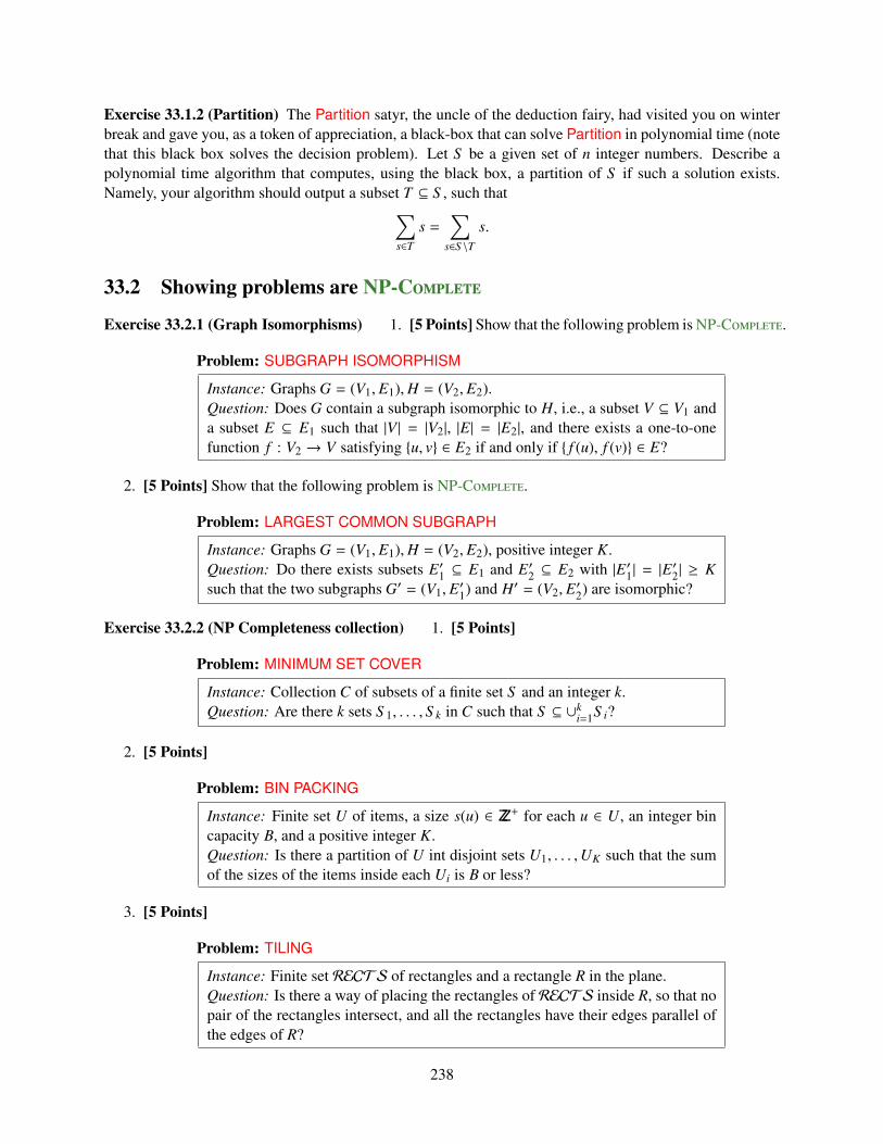
Exercise 33.1.2 (Partition) The Partition satyr, the uncle of the deduction fairy, had visited you on winterbreak and gave you, as a token of appreciation, a black-box that can solve Partition in polynomial time (notethat this black box solves the decision problem). Let S be a given set of n integer numbers. Describe apolynomial time algorithm that computes, using the black box, a partition of S if such a solution exists.Namely, your algorithm should output a subset T ⊆ S , such that∑

s∈T

s =∑

s∈S \T

s.

33.2 Showing problems are NP-C

Exercise 33.2.1 (Graph Isomorphisms) 1. [5 Points] Show that the following problem is NP-C.

Problem: SUBGRAPH ISOMORPHISM

Instance: Graphs G = (V1, E1),H = (V2, E2).Question: Does G contain a subgraph isomorphic to H, i.e., a subset V ⊆ V1 anda subset E ⊆ E1 such that |V | = |V2|, |E| = |E2|, and there exists a one-to-onefunction f : V2 → V satisfying u, v ∈ E2 if and only if f (u), f (v) ∈ E?

2. [5 Points] Show that the following problem is NP-C.

Problem: LARGEST COMMON SUBGRAPH

Instance: Graphs G = (V1, E1),H = (V2, E2), positive integer K.Question: Do there exists subsets E′1 ⊆ E1 and E′2 ⊆ E2 with |E′1| = |E

′2| ≥ K

such that the two subgraphs G′ = (V1, E′1) and H′ = (V2, E′2) are isomorphic?

Exercise 33.2.2 (NP Completeness collection) 1. [5 Points]

Problem: MINIMUM SET COVER

Instance: Collection C of subsets of a finite set S and an integer k.Question: Are there k sets S 1, . . . , S k in C such that S ⊆ ∪k

i=1S i?

2. [5 Points]

Problem: BIN PACKING

Instance: Finite set U of items, a size s(u) ∈ ZZ+ for each u ∈ U, an integer bincapacity B, and a positive integer K.Question: Is there a partition of U int disjoint sets U1, . . . ,UK such that the sumof the sizes of the items inside each Ui is B or less?

3. [5 Points]

Problem: TILING

Instance: Finite set RECTS of rectangles and a rectangle R in the plane.Question: Is there a way of placing the rectangles of RECTS inside R, so that nopair of the rectangles intersect, and all the rectangles have their edges parallel ofthe edges of R?

238

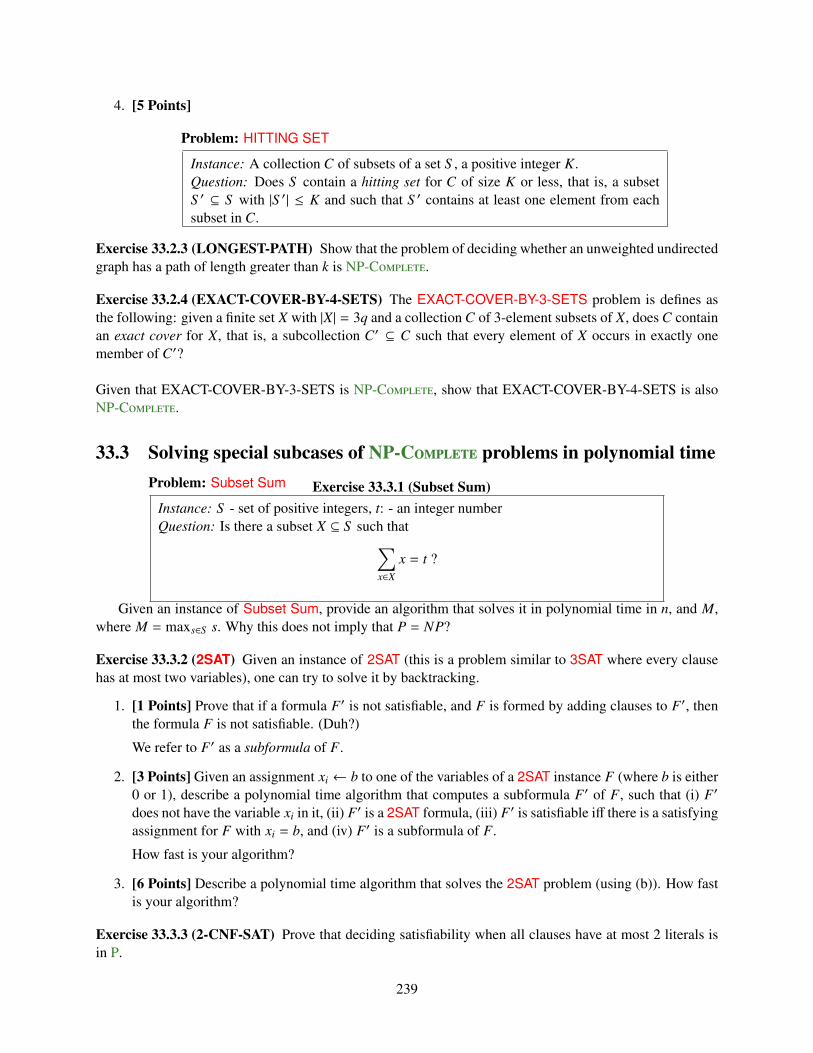
4. [5 Points]

Problem: HITTING SET

Instance: A collection C of subsets of a set S , a positive integer K.Question: Does S contain a hitting set for C of size K or less, that is, a subsetS ′ ⊆ S with |S ′| ≤ K and such that S ′ contains at least one element from eachsubset in C.

Exercise 33.2.3 (LONGEST-PATH) Show that the problem of deciding whether an unweighted undirectedgraph has a path of length greater than k is NP-C.

Exercise 33.2.4 (EXACT-COVER-BY-4-SETS) The EXACT-COVER-BY-3-SETS problem is defines asthe following: given a finite set X with |X| = 3q and a collection C of 3-element subsets of X, does C containan exact cover for X, that is, a subcollection C′ ⊆ C such that every element of X occurs in exactly onemember of C′?

Given that EXACT-COVER-BY-3-SETS is NP-C, show that EXACT-COVER-BY-4-SETS is alsoNP-C.

33.3 Solving special subcases of NP-C problems in polynomial time

Exercise 33.3.1 (Subset Sum)Problem: Subset Sum

Instance: S - set of positive integers, t: - an integer numberQuestion: Is there a subset X ⊆ S such that∑

x∈X

x = t ?

Given an instance of Subset Sum, provide an algorithm that solves it in polynomial time in n, and M,where M = maxs∈S s. Why this does not imply that P = NP?

Exercise 33.3.2 (2SAT) Given an instance of 2SAT (this is a problem similar to 3SAT where every clausehas at most two variables), one can try to solve it by backtracking.

1. [1 Points] Prove that if a formula F′ is not satisfiable, and F is formed by adding clauses to F′, thenthe formula F is not satisfiable. (Duh?)

We refer to F′ as a subformula of F.

2. [3 Points] Given an assignment xi ← b to one of the variables of a 2SAT instance F (where b is either0 or 1), describe a polynomial time algorithm that computes a subformula F′ of F, such that (i) F′

does not have the variable xi in it, (ii) F′ is a 2SAT formula, (iii) F′ is satisfiable iff there is a satisfyingassignment for F with xi = b, and (iv) F′ is a subformula of F.

How fast is your algorithm?

3. [6 Points] Describe a polynomial time algorithm that solves the 2SAT problem (using (b)). How fastis your algorithm?

Exercise 33.3.3 (2-CNF-SAT) Prove that deciding satisfiability when all clauses have at most 2 literals isin P.

239

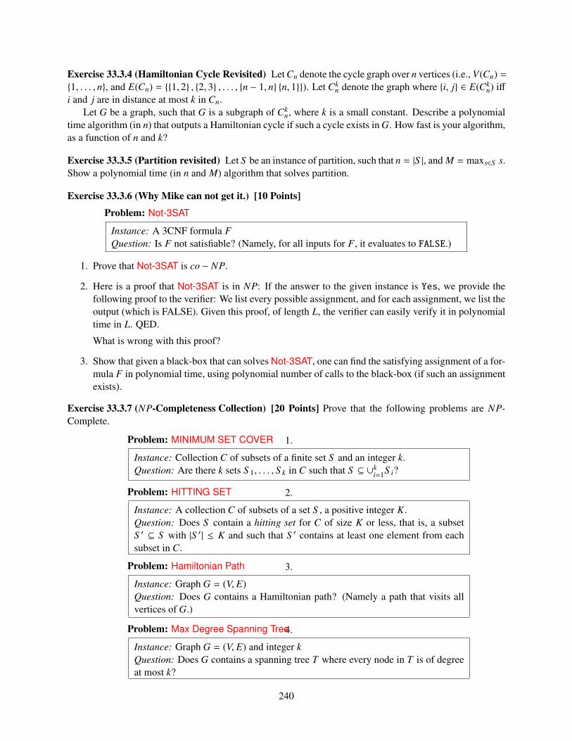
Exercise 33.3.4 (Hamiltonian Cycle Revisited) Let Cn denote the cycle graph over n vertices (i.e., V(Cn) =1, . . . , n, and E(Cn) = 1, 2 , 2, 3 , . . . , n − 1, n n, 1). Let Ck

n denote the graph where i, j ∈ E(Ckn) iff

i and j are in distance at most k in Cn.Let G be a graph, such that G is a subgraph of Ck

n, where k is a small constant. Describe a polynomialtime algorithm (in n) that outputs a Hamiltonian cycle if such a cycle exists in G. How fast is your algorithm,as a function of n and k?

Exercise 33.3.5 (Partition revisited) Let S be an instance of partition, such that n = |S |, and M = maxs∈S s.Show a polynomial time (in n and M) algorithm that solves partition.

Exercise 33.3.6 (Why Mike can not get it.) [10 Points]

Problem: Not-3SAT

Instance: A 3CNF formula FQuestion: Is F not satisfiable? (Namely, for all inputs for F, it evaluates to FALSE.)

1. Prove that Not-3SAT is co − NP.

2. Here is a proof that Not-3SAT is in NP: If the answer to the given instance is Yes, we provide thefollowing proof to the verifier: We list every possible assignment, and for each assignment, we list theoutput (which is FALSE). Given this proof, of length L, the verifier can easily verify it in polynomialtime in L. QED.

What is wrong with this proof?

3. Show that given a black-box that can solves Not-3SAT, one can find the satisfying assignment of a for-mula F in polynomial time, using polynomial number of calls to the black-box (if such an assignmentexists).

Exercise 33.3.7 (NP-Completeness Collection) [20 Points] Prove that the following problems are NP-Complete.

1.Problem: MINIMUM SET COVER


i=1S i?

2.Problem: HITTING SET


3.Problem: Hamiltonian Path

Instance: Graph G = (V, E)Question: Does G contains a Hamiltonian path? (Namely a path that visits allvertices of G.)

4.Problem: Max Degree Spanning Tree

Instance: Graph G = (V, E) and integer kQuestion: Does G contains a spanning tree T where every node in T is of degreeat most k?

240

Exercise 33.3.8 (Independence) [10 Points] Let G = (V, E) be an undirected graph over n vertices. As-sume that you are given a numbering π : V → 1, . . . , n (i.e., every vertex have a unique number), such thatfor any edge i j ∈ E, we have |π(i) − π( j)| ≤ 20.

Either prove that it is NP-Hard to find the largest independent set in G, or provide a polynomial timealgorithm.

Exercise 33.3.9 (Partition) We already know the following problem is NP-C:

Problem: SUBSET SUM

Instance: A finite set A and a “size” s(a) ∈ ZZ+ for each a ∈ A, an integer B.Question: Is there a subset A′ ⊆ A such that

∑a∈A′ s(a) = B?

Now let’s consider the following problem:

Problem: PARTITION

Instance: A finite set A and a “size” s(a) ∈ ZZ+ for each a ∈ A.Question: Is there a subset A′ ⊆ A such that∑

a∈A′s(a) =

∑a∈A\A′

s(a)?

Show that PARTITION is NP-C.

Exercise 33.3.10 (Minimum Set Cover) [15 Points]Problem: MINIMUM SET COVER


i=1S i?

1. [5 Points] Prove that MINIMUM SET COVER problem is NP-C

2. [5 Points] Prove that the following problem is NP-C.



3. [5 Points] Hitting set on the line

Given a set I of n intervals on the real line, show a O(n log n) time algorithm that computes thesmallest set of points X on the real line, such that for every interval I ∈ I there is a point p ∈ X, suchthat p ∈ I.

Exercise 33.3.11 (Bin Packing)Problem: BIN PACKING

Instance: Finite set U of items, a size s(u) ∈ ZZ+ for each u ∈ U, an integer bin capacityB, and a positive integer K.Question: Is there a partition of U into disjoint sets U1, . . . ,UK such that the sum ofthe sizes of the items inside each Ui is B or less?

241

1. [5 Points] Show that the BIN PACKING problem is NP-C


Problem: TILING

Instance: Finite set RECTS of rectangles and a rectangle R in the plane.Question: Is there a way of placing all the rectangles of RECTS inside R, so thatno pair of the rectangles intersect in their interior, and all the rectangles have theiredges parallel of the edges of R?

Exercise 33.3.12 (Knapsack) 1. [5 Points] Show that the following problem is NP-C.

Problem: KNAPSACK

Instance: A finite set U, a "size" s(u) ∈ ZZ+ and a "value" v(u) ∈ ZZ+ for eachu ∈ U, a size constraint B ∈ ZZ+, and a value goal K ∈ ZZ+.Question: Is there a subset U′ ⊆ U such that

∑u∈U′ s(u) ≤ B and

∑u∈U′ v(u) ≥ K.


Problem: MULTIPROCESSOR SCHEDULING

Instance: A finite set A of "tasks", a "length" l(a) ∈ ZZ+ for each a ∈ A, a numberm ∈ ZZ+ of "processors", and a "deadline" D ∈ ZZ+.Question: Is there a partition A = A1

⋃A2

⋃· · ·

⋃Am of A into m disjoint sets

such that max∑

a∈Ai l(a) : 1 ≤ i ≤ m ≤ D?

3. Scheduling with profits and deadlines

Suppose you have one machine and a set of n tasks a1, a2, ..., an. Each task a j has a processing timet j, a profit p j, and a deadline d j. The machine can process only one task at a time, and task a j mustrun uninterruptedly for t j consecutive time units to complete. If you complete task a j by its deadlined j, you receive a profit p j. But you receive no profit if you complete it after its deadline. As anoptimization problem, you are given the processing times, profits and deadlines for a set of n tasks,and you wish to find a schedule that completes all the tasks and returns the greatest amount of profit.

(a) [3 Points] State this problem as a decision problem.(b) [2 Points] Show that the decision problem is NP-C.

Exercise 33.3.13 (Vertex Cover)Problem: VERTEX COVER

Instance: A graph G = (V, E) and a positive integer K ≤ |V |.Question: Is there a vertex cover of size K or less for G, that is, a subset V ′ ⊆ V suchthat |V ′| ≤ K and for each edge u, v ∈ E, at least one of u and v belongs to V ′?

1. Show that VERTEX COVER is NP-C. Hint: Do a reduction from INDEPENDENT SET toVERTEX COVER.

2. Show a polynomial approximation algorithm to the V-C problem which is a factor 2 ap-proximation of the optimal solution. Namely, your algorithm should output a set X ⊆ V , such that Xis a vertex cover, and |C| ≤ 2Kopt, where Kopt is the cardinality of the smallest vertex cover of G.®

®It was very recently shown (I. Dinur and S. Safra. On the importance of being biased. Manuscript.http://www.math.ias.edu/~iritd/mypapers/vc.pdf, 2001.) that doing better than 1.3600 approximation to VERTEXCOVER is NP-Hard. In your free time you can try and improve this constant. Good luck.

242

http://www.math.ias.edu/~iritd/mypapers/vc.pdf

3. Present a linear time algorithm that solves this problem for the case that G is a tree.

4. For a constant k, a graph G is k-separable, if there are k vertices of G, such that if we remove themfrom G, each one of the remaining connected components has at most (2/3)n vertices, and furthermoreeach one of those connected components is also k-separable. (More formally, a graph G = (V, E) isk-separable, if for any subset of vertices S ⊆ V , there exists a subset M ⊆ S , such that each connectedcomponent of GS \M has at most (2/3)|S | vertices, and |M| ≤ k.)

Show that given a graph G which is k-separable, one can compute the optimal VERTEX COVER innO(k) time.

Exercise 33.3.14 (Bin Packing)Problem: BIN PACKING

Instance: Finite set U of items, a size s(u) ∈ ZZ+ for each u ∈ U, an integer bin capacityB, and a positive integer K.Question: Is there a partition of U int disjoint sets U1, . . . ,UK such that the sum of thesizes of the items inside each Ui is B or less?

1. Show that the BIN PACKING problem is NP-C

2. In the optimization variant of BIN PACKING one has to find the minimum number of bins needed tocontain all elements of U. Present an algorithm that is a factor two approximation to optimal solution.Namely, it outputs a partition of U into M bins, such that the total size of each bin is at most B, andM ≤ kopt, where kopt is the minimum number of bins of size B needed to store all the given elementsof U.

3. Assume that B is bounded by an integer constant m. Describe a polynomial algorithm that computesthe solution that uses the minimum number of bins to store all the elements.

4. Show that the following problem is NP-C.

Problem: TILING

Instance: Finite set RECTS of rectangles and a rectangle R in the plane.Question: Is there a way of placing the rectangles of RECTS inside R, so that nopair of the rectangles intersect, and all the rectangles have their edges parallel ofthe edges of R?

5. Assume that RECTS is a set of squares that can be arranged as to tile R completely. Present apolynomial time algorithm that computes a subset T ⊆ RECTS, and a tiling of T , so that this tilingof T covers, say, 10% of the area of R.

Exercise 33.3.15 (Minimum Set Cover)Problem: MINIMUM SET COVER


i=1S i?

1. Prove that MINIMUM SET COVER problem is NP-C

2. The greedy approximation algorithm for MINIMUM SET COVER, works by taking the largest set inX ∈ C, remove all all the elements of X from S and also from each subset of C. The algorithm repeatthis until all the elements of S are removed. Prove that the number of elements not covered after kopt

iterations is at most n/2, where kopt is the smallest number of sets of C needed to cover S , and n = |S |.

243

3. Prove the greedy algorithm is O(log n) factor optimal approximation.

4. Prove that the following problem is NP-C.



5. Given a set I of n intervals on the real line, show a O(n log n) time algorithm that computes thesmallest set of points X on the real line, such that for every interval I ∈ I there is a point p ∈ X, suchthat p ∈ I.

Exercise 33.3.16 (k-Center)Problem: k-CENTER

Instance: A set P of n points in the plane, and an integer k and a radius r.Question: Is there a cover of the points of P by k disks of radius (at most) r?

1. Describe an nO(k) time algorithm that solves this problem.

2. There is a very simple and natural algorithm that achieves a 2-approximation for this cover: First itselect an arbitrary point as a center (this point is going to be the center of one of the k covering disks).Then it computes the point that it furthest away from the current set of centers as the next center, andit continue in this fashion till it has k-points, which are the resulting centers. The smallest k equalradius disks centered at those points are the required k disks.

Show an implementation of this approximation algorithm in O(nk) time.

3. Prove that that the above algorithm is a factor two approximation to the optimal cover. Namely, theradius of the disks output ≤ 2ropt, where ropt is the smallest radius, so that we can find k-disks thatcover the point-set.

4. Provide an ε-approximation algorithm for this problem. Namely, given k and a set of points P in theplane, your algorithm would output k-disks that cover the points and their radius is ≤ (1+ε)ropt, whereropt is the minimum radius of such a cover of P.

5. Prove that dual problem r-DISK-COVER problem is NP-Hard. In this problem, given P and a radiusr, one should find the smallest number of disks of radius r that cover P.

6. Describe an approximation algorithm to the r-DISK COVER problem. Namely, given a point-set Pand a radius r, outputs k disks, so that the k disks cover P and are of radius r, and k = O(kopt), wherekopt is the minimal number of disks needed to cover P by disks of radius r.

Exercise 33.3.17 (MAX 3SAT) Consider the Problem MAX SAT.

Problem: MAX SAT

Instance: Set U of variables, a collection C of disjunctive clauses of literals where aliteral is a variable or a negated variable in U.Question: Find an assignment that maximized the number of clauses of C that arebeing satisfied.

244

1. Prove that MAX SAT is NP-Hard.

2. Prove that if each clause has exactly three literals, and we randomly assign to the variables values 0or 1, then the expected number of satisfied clauses is (7/8)M, where M = |C|.

3. Show that for any instance of MAX SAT, where each clause has exactly three different literals, thereexists an assignment that satisfies at least 7/8 of the clauses.

4. Let (U,C) be an instance of MAX SAT such that each clause has ≥ 10 · log n distinct variables, wheren is the number of clauses. Prove that there exists a satisfying assignment. Namely, there exists anassignment that satisfy all the clauses of C.

Exercise 33.3.18 (Complexity) 1. Prove that P ⊆ -NP.

2. Show that if NP , -NP, then every NP-C problem is not a member of -NP.

Exercise 33.3.19 (3SUM) Describe an algorithm that solves the following problem as quickly as possible:Given a set of n numbers, does it contain three elements whose sum is zero? For example, your algorithmshould answer T for the set −5,−17, 7,−4, 3,−2, 4, since −5 + 7 + (−2) = 0, and F for the set−6, 7,−4,−13,−2, 5, 13.

Exercise 33.3.20 (Polynomially equivalent.) Consider the following pairs of problems:

1. MIN SPANNING TREE and MAX SPANNING TREE

2. SHORTEST PATH and LONGEST PATH

3. TRAVELING SALESMAN PROBLEM and VACATION TOUR PROBLEM (the longest tour issought).

4. MIN CUT and MAX CUT (between s and t)

5. EDGE COVER and VERTEX COVER

6. TRANSITIVE REDUCTION and MIN EQUIVALENT DIGRAPH

(all of these seem dual or opposites, except the last, which are just two versions of minimal representationof a graph).

Which of these pairs are polytime equivalent and which are not? Why?

Exercise 33.3.21 (PLANAR-3-COLOR) Using 3COLORABLE, and the ‘gadget’ in figure 33.3.21, provethat the problem of deciding whether a planar graph can be 3-colored is NP-C. Hint: show that thegadget can be 3-colored, and then replace any crossings in a planar embedding with the gadget appropriately.

Exercise 33.3.22 (DEGREE-4-PLANAR-3-COLOR) Using the previous result, and the ‘gadget’ in figure33.3.22, prove that the problem of deciding whether a planar graph with no vertex of degree greater thanfour can be 3-colored is NP-C. Hint: show that you can replace any vertex with degree greater than4 with a collection of gadgets connected in such a way that no degree is greater than four.

245

Figure 33.1: Gadget for PLANAR-3-COLOR.

Figure 33.2: Gadget for DEGREE-4-PLANAR-3-COLOR.

Exercise 33.3.23 (Primality and Complexity) Prove that PRIMALITY (Given n, is n prime?) is in NP ∩-NP. Hint: -NP is easy (what’s a certificate for showing that a number is composite?). For NP, considera certificate involving primitive roots and recursively their primitive roots. Show that knowing this tree ofprimitive roots can be checked to be correct and used to show that n is prime, and that this check takes polytime.

Exercise 33.3.24 (Poly time subroutines can lead to exponential algorithms) Show that an algorithm thatmakes at most a constant number of calls to polynomial-time subroutines runs in polynomial time, but thata polynomial number of calls to polynomial-time subroutines may result in an exponential-time algorithm.

Exercise 33.3.25 (Polynomial time Hmiltonian path) 1. Prove that if G is an undirected bipartite graphwith an odd number of vertices, then G is nonhamiltonian. Give a polynomial time algorithm algo-rithm for finding a hamiltonian cycle in an undirected bipartite graph or establishing that it does notexist.

2. Show that the hamiltonian-path problem can be solved in polynomial time on directed acyclic graphsby giving an efficient algorithm for the problem.

3. Explain why the results in previous questions do not contradict the facts that both HAM-CYCLE andHAM-PATH are NP-C problems.

Exercise 33.3.26 ((Really Hard)GRAPH-ISOMORPHISM) Consider the problem of deciding whetherone graph is isomorphic to another.

1. Give a brute force algorithm to decide this.

2. Give a dynamic programming algorithm to decide this.

3. Give an efficient probabilistic algorithm to decide this.

4. Either prove that this problem is NP-C, give a poly time algorithm for it, or prove that neithercase occurs.

246

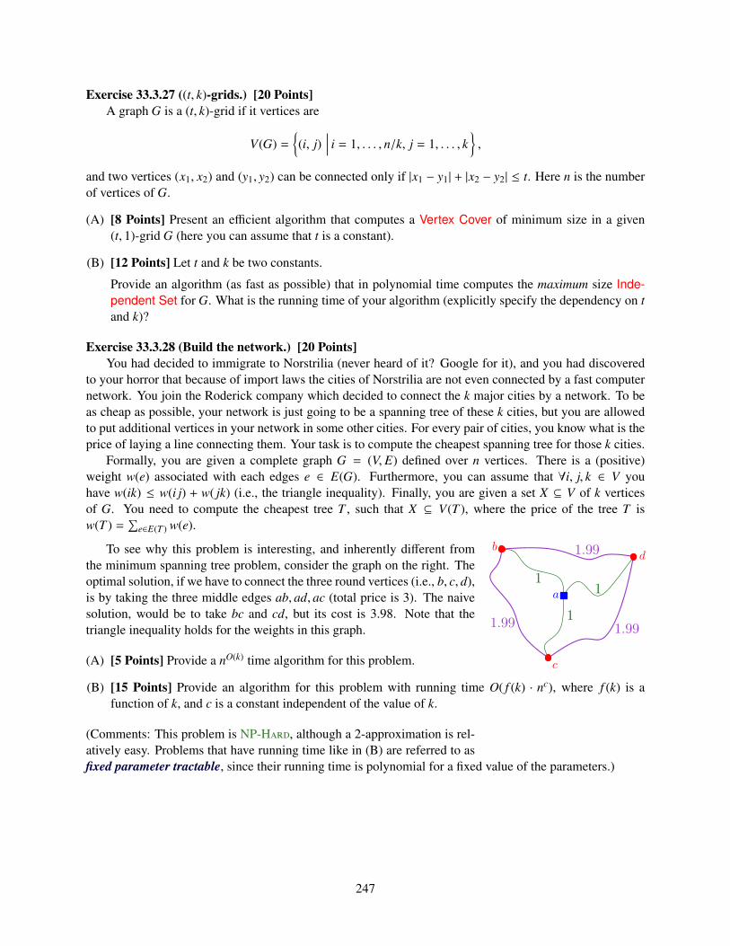
Exercise 33.3.27 ((t, k)-grids.) [20 Points]A graph G is a (t, k)-grid if it vertices are

V(G) =(i, j)

∣∣∣∣ i = 1, . . . , n/k, j = 1, . . . , k,

and two vertices (x1, x2) and (y1, y2) can be connected only if |x1 − y1| + |x2 − y2| ≤ t. Here n is the numberof vertices of G.

(A) [8 Points] Present an efficient algorithm that computes a Vertex Cover of minimum size in a given(t, 1)-grid G (here you can assume that t is a constant).

(B) [12 Points] Let t and k be two constants.

Provide an algorithm (as fast as possible) that in polynomial time computes the maximum size Inde-pendent Set for G. What is the running time of your algorithm (explicitly specify the dependency on tand k)?

Exercise 33.3.28 (Build the network.) [20 Points]You had decided to immigrate to Norstrilia (never heard of it? Google for it), and you had discovered

to your horror that because of import laws the cities of Norstrilia are not even connected by a fast computernetwork. You join the Roderick company which decided to connect the k major cities by a network. To beas cheap as possible, your network is just going to be a spanning tree of these k cities, but you are allowedto put additional vertices in your network in some other cities. For every pair of cities, you know what is theprice of laying a line connecting them. Your task is to compute the cheapest spanning tree for those k cities.

Formally, you are given a complete graph G = (V, E) defined over n vertices. There is a (positive)weight w(e) associated with each edges e ∈ E(G). Furthermore, you can assume that ∀i, j, k ∈ V youhave w(ik) ≤ w(i j) + w( jk) (i.e., the triangle inequality). Finally, you are given a set X ⊆ V of k verticesof G. You need to compute the cheapest tree T , such that X ⊆ V(T ), where the price of the tree T isw(T ) =

∑e∈E(T ) w(e).

11

1

1.99

1.991.99

a

b

c

dTo see why this problem is interesting, and inherently different from

the minimum spanning tree problem, consider the graph on the right. Theoptimal solution, if we have to connect the three round vertices (i.e., b, c, d),is by taking the three middle edges ab, ad, ac (total price is 3). The naivesolution, would be to take bc and cd, but its cost is 3.98. Note that thetriangle inequality holds for the weights in this graph.

(A) [5 Points] Provide a nO(k) time algorithm for this problem.

(B) [15 Points] Provide an algorithm for this problem with running time O( f (k) · nc), where f (k) is afunction of k, and c is a constant independent of the value of k.

(Comments: This problem is NP-H, although a 2-approximation is rel-atively easy. Problems that have running time like in (B) are referred to asfixed parameter tractable, since their running time is polynomial for a fixed value of the parameters.)

247

248

Chapter 34

Exercises - Network Flow

This chapter include problems that are realted to network flow.

34.1 Network Flow

Exercise 34.1.1 (The good, the bad, and the middle.) [10 Points]Suppose you’re looking at a flow network G with source s and sink t, and you want to be able to express

something like the following intuitive notion: Some nodes are clearly on the “source side” of the mainbottlenecks; some nodes are clearly on the “sink side” of the main bottlenecks; and some nodes are in themiddle. However, G can have many minimum cuts, so we have to be careful in how we try making this ideaprecise.

Here’s one way to divide the nodes of G into three categories of this sort.

• We say a node v is upstream if, for all minimum s-t cuts (A, B), we have v ∈ A – that is, v lies on thesource side of every minimum cut.

• We say a node v is downstream if, for all minimum s-t cuts (A, B), we have v ∈ B – that is, v lies onthe sink side of every minimum cut.

• We say a node v is central if it is neither upstream nor downstream; there is at least one minimums-t cut (A, B) for which v ∈ A, and at least one minimum s-t cut (A′, B′) for which v ∈ B′.

Give an algorithm that takes a flow network G and classifies each of its nodes as being upstream, down-stream, or central. The running time of your algorithm should be within a constant factor of the time requiredto compute a single maximum flow.

Exercise 34.1.2 (Ad hoc networks) [20 Points]Ad hoc networks are made up of low-powered wireless devices, have been proposed for situations like

natural disasters in which the coordinators of a rescue effort might want to monitor conditions in a hard-to-reach area. The idea is that a large collection of these wireless devices could be dropped into such an areafrom an airplane and then configured into a functioning network.

Note that we’re talking about (a) relatively inexpensive devices that are (b) being dropped from an air-plane into (c) dangerous territory; and for the combination of reasons (a), (b), and (c), it becomes necessaryto include provisions for dealing with the failure of a reasonable number of the nodes.

We’d like it to be the case that if one of the devices v detects that it is in danger of failing, it shouldtransmit a representation of its current state to some other device in the network. Each device has a limited

249

transmitting range – say it can communicate with other devices that lie within d meters of it. Moreover,since we don’t want it to try transmitting its state to a device that has already failed, we should include someredundancy: A device v should have a set of k other devices that it can potentially contact, each within dmeters of it. We’ll call this a back-up set for device v.

1. Suppose you’re given a set of n wireless devices, with positions represented by an (x, y) coordinatepair for each. Design an algorithm that determines whether it is possible to choose a back-up setfor each device (i.e., k other devices, each within d meters), with the further property that, for someparameter b, no device appears in the back-up set of more than b other devices. The algorithm shouldoutput the back-up sets themselves, provided they can be found.

2. The idea that, for each pair of devices v and w, there’s a strict dichotomy between being “in range” or“out of range” is a simplified abstraction. More accurately, there’s a power decay function f (·) thatspecifies, for a pair of devices at distance δ, the signal strength f (δ) that they’ll be able to achieve ontheir wireless connection. (We’ll assume that f (δ) decreases with increasing δ.)

We might want to build this into our notion of back-up sets as follows: among the k devices in theback-up set of v, there should be at least one that can be reached with very high signal strength, at leastone other that can be reached with moderately high signal strength, and so forth. More concretely,we have values p1 ≥ p2 ≥ · · · ≥ pk, so that if the back-up set for v consists of devices at distancesd1 ≤ d2 ≤ · · · ≤ dk, then we should have f (d j) ≥ p j for each j.

Give an algorithm that determines whether it is possible to choose a back-up set for each device subjectto this more detailed condition, stil requiring that no device should appear in the back-up set of morethan b other devices. Again, the algorithm should output the back-up sets themselves, provided theycan be found.

Exercise 34.1.3 (Minimum Flow) [10 Points]Give a polynomial-time algorithm for the following minimization analogue of the Maximum-Flow Prob-

lem. You are given a directed graph G = (V, E), with a source s ∈ V and sink t ∈ V , and numbers (capacities)`(v,w) for each edge (v,w) ∈ E. We define a flow f , and the value of a flow, as usual, requiring that allnodes except s and t satisfy flow conservation. However, the given numbers are lower bounds on edge flow– that is, they require that f (v,w) ≥ `(v,w) for every edge (v,w) ∈ E, and there is no upper bound on flowvalues on edges.

1. Give a polynomial-time algorithm that finds a feasible flow of minimum possible values.

2. Prove an analogue of the Max-Flow Min-Cut Theorem for this problem (i.e., does min-flow = max-cut?).

Exercise 34.1.4 (Prove infeasibility.) You are trying to solve a circulation problem, but it is not feasible.The problem has demands, but no capacity limits on the edges. More formally, there is a graph G = (V, E),and demands dv for each node v (satisfying

∑v∈V dv = 0), and the problem is to decide if there is a flow f

such that f (e) ≥ 0 and f in(v)− f out(v) = dv for all nodes v ∈ V . Note that this problem can be solved via thecirculation algorithm from Section 7.7 by setting ce = +∞ for all edges e ∈ E. (Alternately, it is enough toset ce to be an extremely large number for each edge – say, larger than the total of all positive demands dv inthe graph.)

You want to fix up the graph to make the problem feasible, so it would be very useful to know why theproblem is not feasible as it stands now. On a closer look, you see that there is a subset U of nodes such thatthere is no edge into U, and yet

∑v∈U dv > 0. You quickly realize that the existence of such a set immediately

implies that the flow cannot exist: The set U has a positive total demand, and so needs incoming flow, and

250

yet U has no edges into it. In trying to evaluate how far the problem is from being solvable, you wonderhow big the demand of a set with no incoming edges can be.

Give a polynomial-time algorithm to find a subset S ⊂ V of nodes such that there is no edge into S andfor which

∑v∈S dv is as large as possible subject to this condition.

Exercise 34.1.5 (Cellphones and services.) Consider an assignment problem where we have a set of nstations that can provide service, and there is a set of k requests for service. Say, for example, that thestations are cell towers and the requests are cell phones. Each request can be served by a given set ofstations. The problem so far can be represented by a bipartite graph G: one side is the stations, the otherthe customers, and there is an edge (x, y) between customer x and station y if customer x can be served fromstation y. Assume that each station can serve at most one customer. Using a max-flow computation, wecan decide whether or not all customers can be served, or can get an assignment of a subset of customers tostations maximizing the number of served customers.

Here we consider a version of the problem with an addition complication: Each customer offers adifferent amount of money for the service. Let U be the set of customers, and assume that customer x ∈ Uis willing to pay vx ≥ 0 for being served. Now the goal is to find a subset X ⊂ U maximizing

∑x∈X vx such

that there is an assignment of the customers in X to stations.Consider the following greedy approach. We process customers in order of decreasing value (breaking

ties arbitrarily). When considering customer x the algorithm will either “promise” service to x or reject xin the following greedy fasion. Let X be the set of customers that so far have been promised service. Weadd x to the set X if and only if there is a way to assign X ∪ x to servers, and we reject x otherwise. Notethat rejected customers will not be considered later. (This is viewed as an advantage: If we need to reject ahigh-paying customer, at least we can tell him/her early.) However, we do not assign accepting customersto servers in a greedy fasion: we only fix the assignment after the set of accepted customers is fixed. Doesthis greedy approach produce an optimal set of customers? Prove that it does, or provide a counterexample.

Exercise 34.1.6 (Follow the stars) [20 Points]Some friends of yours have grown tired of the game “Six Degrees of Kevin Bacon” (after all, they ask,

isn’t it just breadth-first search?) and decide to invent a game with a little more punch, algorithmicallyspeaking. Here’s how it works.

You start with a set X of n actresses and a set Y of n actors, and two players P0 and P1. Player P0names an actress x1 ∈ X, player P1 names an actor y1 who has appeared in a movie with x1, player P0names an actress x2 who has appeared in a movie with y1, and so on. Thus, P0 and P1 collectively generatea sequence x1, y1, x2, y2, . . . such that each actor/actress in the sequence has costarred with the actress/actorimmediately preceding. A player Pi (i = 0, 1) loses when it is Pi’s turn to move, and he/she cannot name amember of his/her set who hasn’t been named before.

Suppose you are given a specific pair of such sets X and Y , with complete information on who hasappeared in a movie with whom. A strategy for Pi, in our setting, is an algorithm that takes a currentsequence x1, y1, x2, y2, . . . and generates a legal next move for Pi (assuming it’s Pi’s turn to move). Give apolynomial-time algorithm that decides which of the two players can force a win, in a particular instance ofthis game.

Exercise 34.1.7 (Flooding) [10 Points]Network flow issues come up in dealing with natural disasters and other crises, since major unexpected

events often require the movement and evacuation of large numbers of people in a short amount of time.Consider the following scenario. Due to large-scale flooding in a region, paramedics have identified a

set of n injured people distributed across the region who need to be rushed to hospitals. There are k hospitalsin the region, and each of the n people needs to be brought to a hospital that is within a half-hour’s driving

251

time of their current location (so different people will have different options for hospitals, depending onwhere they are right now).

At the same time, one doesn’t want to overload any one of the hospitals by sending too many patientsits way. The paramedics are in touch by cell phone, and they want to collectively work out whether theycan choose a hospital for each of the injured people in such a way that the load on the hospitals is balanced:Each hospital receives at most dn/ke people.

Give a polynomial-time algorithm that takes the given information about the people’s locations anddetermines whether this is possible.

Exercise 34.1.8 (Capacitation, yeh, yeh, yeh) Suppose you are given a directed graph G = (V, E), with apositive integer capacity ce on each edge e, a designated source s ∈ V , and a designated sink t ∈ V . You arealso given a maximum s-t flow in G, defined by a flow value fe on each edge e. The flow fe is acyclic:There is no cycle in G on which all edges carry positive flow.

Now suppose we pick a specific edge e∗ ∈ E and reduce its capacity by 1 unit. Show how to find amaximum flow in the resulting capacitated graph in time O(m+n), where m is the number of edges in G andn is the number of nodes.

Exercise 34.1.9 (Fast Friends) [20 Points]Your friends have written a very fast piece of maximum-flow code based on repeatedly finding augment-

ing paths as in the course lecture notes. However, after you’ve looked at a bit of output from it, you realizethat it’s not always finding a flow of maximum value. The bug turns out to be pretty easy to find; your friendshadn’t really gotten into the whole backward-edge thing when writing the code, and so their implementationbuilds a variant of the residual graph that only includes the forwards edges. In other words, it searches fors-t paths in a graph G f consisting only of edges of e for which f (e) < ce, and it terminates when there is noaugmenting path consisting entirely of such edges. We’ll call this the Forward-Edge-Only Algorithm. (Notethat we do not try ot prescribe how this algorithms chooses its forward-edge paths; it may choose them inany fashion it wants, provided that it terminates only when there are no forward-edge paths.)

It’s hard to convince your friends they need to reimplement the code. In addition to its blazing speed,they claim, in fact, that it never returns a flow whose value is less than a fixed fraction of optimal. Do youbelieve this? The crux of their claim can be made precise in the following statement.

“There is an absolute constant b > 1 (independent of the particular input flow network), so that on everyinstance of the Maximum-Flow Problem, the Forward-Edge-Only Algorithm is guaranteed to find a flow ofvalue at least 1/b times the maximum-flow value (regardless of how it chooses its forward-edge paths).

Decide whether you think this statement is true or false, and give a proof of either the statement or itsnegation.

Exercise 34.1.10 (Even More Capacitation) [10 Points]In a standard s − t Maximum-Flow Problem, we assume edges have capacities, and there is no limit on

how much flow is allowed to pass through a node. In this problem, we consider the variant of the Maximum-Flow and Minimum-Cut problems with node capacities.

Let G = (V, E) be a directed graph, with source s ∈ V , sink t ∈ V , and nonnegative node capacitiescv ≥ 0 for each v ∈ V . Given a flow f in this graph, the flow through a node v is defined as f in(v). We saythat a flow is feasible if it satisfies the usual flow-conservation constraints and the node-capacity constraints:f in(v) ≤ cv for all nodes.

Give a polynomial-time algorithm to find an s-t maximum flow in such a node-capacitated network.Define an s-t cut for node-capacitated networks, and show that the analogue of the Max-Flow Min-CutTheorem holds true.

252

Exercise 34.1.11 (Matrices) [10 Points]Let M be an n × n matrix with each entry equal to either 0 or 1. Let mi j denote the entry in row i and

column j. A diagonal entry is one of the form mii for some i.

1. [2 Points] Give an example of a matrix M that is not rearrangeable, but for which at least one entry ineach row and each column is equal to 1.

2. [8 Points] Give a polynomial-time algorithm that determines whether a matrix M with 0-1 entries isrearrangeable.

Exercise 34.1.12 (Unique Cut) [10 Points]Let G = (V, E) be a directed graph, with source s ∈ V , sink t ∈ V , and nonnegative edge capacities ce.

Give a polynomial-time algorithm to decide whether G has a unique minimum s-t cut (i.e., an s-t of capacitystrictly less than that of all other s-t cuts).

Exercise 34.1.13 (Transitivity) [10 Points]Given a graph G = (V, E), and a natural number k, we can define a relation

G,k−−→ on pairs of vertices of G

as follows. If x, y ∈ V , we say that xG,k−−→ y if there exist k mutually edge-disjoint paths from x to y in G.

Is it true that for every G and every k ≥ 0, the relationG,k−−→ is transitive? That is, is it always the case

that if xG,k−−→ y and y

G,k−−→ z, then we have x

G,k−−→ z? Give a proof or a counterexample.

Exercise 34.1.14 (Census Rounding) [20 Points]You are consulting for an environmental statistics firm. They collect statistics and publish the collected

data in a book. The statistics are about populations of different regions in the world and are recorded inmultiples of one million. Examples of such statistics would look like the following table.

Country A B C Totalgrown-up men 11.998 9.083 2.919 24.000grown-up women 12.983 10.872 3.145 27.000children 1.019 2.045 0.936 4.000total 26.000 22.000 7.000 55.000

We will assume here for simplicity that our data is such that all row and column sums are integers. TheCensus Rounding Problem is to round all data to integers without changing any row or column sum. Eachfractional number can be rounded either up or down. For example, a good rounding for our table data wouldbe as follows.

Country A B C Totalgrown-up men 11.000 10.000 3.000 24.000grown-up women 13.000 10.000 4.000 27.000children 1.000 2.000 0.000 4.000total 26.000 22.000 7.000 55.000

1. [5 Points] Consider first the special case when all data are between 0 and 1. So you have a matrix offractional numbers between 0 and 1, and your problem is to round each fraction that is between 0 and1 to either 0 or 1 without changing the row or column sums. Use a flow computation to check if thedesired rounding is possible.

2. [5 Points] Consider the Census Rounding Problem as defined above, where row and column sums areintegers, and you want to round each fractional number α to either bαc or dαe. Use a flow computationto check if the desired rounding is possible.

253

3. [10 Points] Prove that the rounding we are looking for in (a) and (b) always exists.

Exercise 34.1.15 (Edge Connectivity) [20 Points]The edge connectivity of an undirected graph is the minimum number k of edges that must be removed

to disconnect the graph. For example, the edge connectivity of a tree is 1, and the edge connectivity of acyclic chain of vertices is 2. Show how the edge connectivity of an undirected graph G = (V, E) can bedetermined by running a maximum-flow algorithm on at most |V | flow networks, each having O(V) verticesand O(E) edges.

Exercise 34.1.16 (Maximum Flow By Scaling) [20 Points]Let G = (V, E) be a flow network with source s, sink t, and an integer capacity c(u, v) on each edge

(u, v) ∈ E. Let C = max(u,v)∈Ec(u, v).

1. [2 Points] Argue that a minimum cut of G has capacity at most C|E|.

2. [5 Points] For a given number K, show that an augmenting path of capacity at least K can be foundin O(E) time, if such a path exists.

The following modification of F-F-M can be used to compute a maximum flow inG.

M-F-B-S(G, s, t)1 C ← max(u,v)∈Ec(u, v)2 initialize flow f to 03 K ← 2blg Cc

4 while K ≥ 1 do 5 while (there exists an augmenting path p of

capacity at least K) do 6 augment flow f along p

7 K ← K/2

8 return f

3. [3 Points] Argue that M-F-B-S returns a maximum flow.

4. [4 Points] Show that the capacity of a minimum cut of the residual graph G f is at most 2K|E| eachtime line 4 is executed.

5. [4 Points] Argue that the inner while loop of lines 5-6 is executed O(E) times for each value of K.

6. [2 Points] Conclude that M-F-B-S can be implemented so that it runs in O(E2 lg C)time.

Exercise 34.1.17 (Perfect Matching) [20 Points]

1. [10 Points] A perfect matching is a matching in which every vertex is matched. Let G = (V, E) be anundirected bipartite graph with vertex partition V = L ∪ R, where |L| = |R|. For any X ⊆ V , define theneighborhood of X as

N(X) =y ∈ V

∣∣∣∣ (x, y) ∈ E for some x ∈ X,

254

that is, the set of vertices adjacent to some member of X. Prove Hall’s theorem: there exists a perfectmatching in G if and only if |A| ≤ |N(A)| for every subset A ⊆ L.

2. [10 Points] We say that a bipartite graph G = (V, E), where V = L ∪ R, is d-regular if every vertexv ∈ V has degree exactly d. Every d-regular bipartite graph has |L| = |R|. Prove that every d-regularbipartite graph has a matching of cardinality |L| by arguing that a minimum cut of the correspondingflow network has capacity |L|.

Exercise 34.1.18 (Number of augmneting paths) 1. [10 Points] Show that a maximum flow in a net-work G = (V, E) can always be found by a sequence of at most |E| augmenting paths. [Hint: Determinethe paths after finding the maximum flow.]

2. [10 Points] Suppose that a flow network G = (V, E) has symmetric edges, that is, (u, v) ∈ E if andonly (v, u) ∈ E. Show that the Edmonds-Karp algorithm terminates after at most |V ||E|/4 iterations.[Hint: For any edge (u,v), consider how both δ(s, u) and δ(v, t) change between times at which (u,v)is critical.]

Exercise 34.1.19 (Minimum Cut Festival) [20 Points]

1. Given a multigraph G(V, E), show that an edge can be selected uniform at random from E in timeO(n), given access to a source of random bits.

2. For any α ≥ 1, define an α approximate cut in a multigraph G as any cut whose cardinality is withina multiplicative factor α of the cardinality of the min-cut in G. Determine the probability that a singleiteration of the randomized algorithm for cuts will produce as output some α-approximate cut in G.

3. Using the analysis of the randomized min-cut algorithm, show that the number of distinct min-cuts ina multigraph G cannot exceed n(n − 1)/2, where n is the number of vertices in G.

4. Formulate and prove a similar result of the number of α -approximate cuts in a multigraph G.

Exercise 34.1.20 (Independence Matrix) [10 Points]Consider a 0 − 1 matrix H with n1 rows and n2 columns. We refer to a row or a column of the matrix H

as a line. We say that a set of 1’s in the matrix H is independent if no two of them appear in the same line.We also say that a set of lines in the matrix is a cover of H if they include (i.e., “cover”) all the 1’s in thematrix. Using the max-flow min-cut theorem on an appropriately defined network, show that the maximumnumber of independent 1’s equals the minimum number of lines in the cover.

Exercise 34.1.21 (Scalar Flow Product) [10 Points]Let f be a flow in a network, and let α be a real number. The scalar flow product, denoted by α f , is a

function from V × V to IR defined by(α f )(u, v) = α · f (u, v).

Prove that the flows in a network form a convex set. That is, show that if f1 and f2 are flows, then so isα f1 + (1 − α) f2 for all α in the range 0 ≤ α ≤ 1.

Exercise 34.1.22 (Go to school!) Professor Adam has two children who, unfortunately, dislike each other.The problem is so severe that not only they refuse to walk to school together, but in fact each one refusesto walk on any block that the other child has stepped on that day. The children have no problem with theirpaths crossing at a corner. Fortunately both the professor’s house and the school are on corners, but beyondthat he is not sure if it is going to be possible to send both of his children to the same school. The professorhas a map of his town. Show how to formulate the problem of determining if both his children can go to thesame school as a maximum-flow problem.

255

Exercise 34.1.23 (The Hopcroft-Karp Bipartite Matching Algorithm) [20 Points]In this problem, we describe a faster algorithm, due to Hopcroft and Karp, for finding a maximum

matching in a bipartite graph. The algorithm runs in O(√

VE) time. Given an undirected, bipartite graphG = (V, E), where V = L ∪ R and all edges have exactly one endpoint in L, let M be a matching in G. Wesay that a simple path P in G is an augmenting path with respect to M if it starts at an unmatched vertex inL, ends at an unmatched vertex in R, and its edges belong alternatively to M and E − M. (This definition ofan augmenting path is related to, but different from, an augmenting path in a flow network.) In this problem,we treat a path as a sequence of edges, rather than as a sequence of vertices. A shortest augmenting pathwith respect to a matching M is an augmenting path with a minimum number of edges.

Given two sets A and B, the symmetric difference A ⊕ B is defined as (A − B) ∪ (B − A), that is, theelements that are in exactly one of the two sets.

1. [4 Points] Show that if M is a matching and P is an augmenting path with respect to M, then thesymmetric difference M⊕P is a matching and |M⊕P| = |M|+1. Show that if P1, P2, ..., Pk are vertex-disjoint augmenting paths with respect to M, then the symmetric difference M ⊕ (P1 ∪ P2 ∪ ... ∪ Pk)is a matching with cardinality |M| + k.

The general structure of our algorithm is the following:

H-K(G)1 M ← ∅2 repeat3 let P← P1, P2, ..., Pk be a maximum set of

vertex-disjoint shortest augmenting pathswith respect to M

4 M ← M ⊕ (P1 ∪ P2 ∪ . . . ∪ Pk)5 until P = ∅

6 return M

The remainder of this problem asks you to analyze the number of iterations in the algorithm (that is,the number of iterations in the repeat loop) and to describe an implementation of line 3.

2. [4 Points] Given two matchings M and M∗ in G, show that every vertex in the graph G′ = (V,M⊕M∗)has degree at most 2. Conclude that G′ is a disjoint union of simple paths or cycles. Argue that edgesin each such simple path or cycle belong alternatively to M or M∗. Prove that if |M| ≤ |M∗|, thenM ⊕ M∗ contains at least |M∗| − |M| vertex-disjoint augmenting paths with respect to M.

Let l be the length of a shortest augmenting path with respect to a matching M, and let P1, P2,..., Pk be a maximum set of vertex-disjoint augmenting paths of length l with respect to M. LetM′ = M ⊕ (P1 ∪ P2 ∪ ... ∪ Pk), and suppose that P is a shortest augmenting path with respect to M′.

3. [2 Points] Show that if P is vertex-disjoint from P1, P2, ..., Pk, then P has more than l edges.

4. [2 Points] Now suppose P is not vertex-disjoint from P1, P2, ..., Pk. Let A be the set of edges(M ⊕ M′) ⊕ P. Show that A = (P1 ∪ P2 ∪ ... ∪ Pk) ⊕ P and that |A| ≥ (k + 1)l. Conclude that P hasmore than l edges.

5. [2 Points] Prove that if a shortest augmenting path for M has length l, the size of the maximummatching is at most |M| + |V |/l.

256

6. [2 Points] Show that the number of repeat loop iterations in the algorithm is at most 2√

V . [Hint: Byhow much can M grow after iteration number

√V?]

7. [4 Points] Give an algorithm that runs in O(E) time to find a maximum set of vertex-disjoint shortestaugmenting paths P1, P2, ..., Pk for a given matching M. Conclude that the total running time ofH-K is O(

√VE).

34.2 Min Cost Flow

Exercise 34.2.1 (Streaming TV.) [20 Points]You are given a directed graph G, a source vertex s (i.e., a server in the internet), and a set T of vertices

(i.e., consumers computers). We would like to broadcast as many TV programs from the server to thecustomers simultaneously. A single broadcast is a path from the server to one of the customers. Theconstraint is that no edge or vertex (except from the server) can have two streams going through them.

(A) [10 Points] Provide a polynomial time algorithm that computes the largest number of paths that can bestreamed from the server.

(B) [10 Points] Let k be the number of paths computed in (A). Present an algorithm, that in polynomialtime, computes a set of k such paths (one end point in the server, the other endpoint is in T ) withminimum number of edges.

Exercise 34.2.2 (T P.) [20 Points]Let G be a digraph with n vertices and m edges.In the transportation problem, you are given a set X of x vertices in a graph G, for every vertex v ∈ X

there is a quantity qx > 0 of material available at v. Similarly, there is a set of vertices Y , with associatedcapacities cy with each vertex y ∈ Y . Furthermore, every edge of G has an associated distance with it.

The work involved in transporting α units of material on an edge e of length ` is α ∗ `. The problem isto move all the material available in X to the vertices of Y , without violating the capacity constraints of thevertices, while minimizing the overall work involved.

Provide a polynomial time algorithm for this problem. How fast is your algorithm?

Exercise 34.2.3 (Edge Connectivity) [20 Points]The edge connectivity of an undirected graph is the minimum number k of edges that must be removed

to disconnect the graph. For example, the edge connectivity of a tree is 1, and the edge connectivity of acyclic chain of vertices is 2. Show how the edge connectivity of an undirected graph G = (V, E) can bedetermined by running a maximum-flow algorithm on at most |V | flow networks, each having O(V) verticesand O(E) edges.

Exercise 34.2.4 (Maximum Flow By Scaling) [20 Points]Let G = (V, E) be a flow network with source s, sink t, and an integer capacity c(u, v) on each edge

(u, v) ∈ E. Let C = max(u,v)∈Ec(u, v).

1. [2 Points] Argue that a minimum cut of G has capacity at most C|E|.

2. [5 Points] For a given number K, show that an augmenting path of capacity at least K can be foundin O(E) time, if such a path exists.

The following modification of F-F-M can be used to compute a maximum flow inG.

257

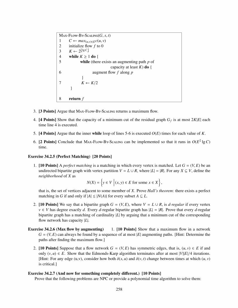
M-F-B-S(G, s, t)1 C ← max(u,v)∈Ec(u, v)2 initialize flow f to 03 K ← 2blg Cc

4 while K ≥ 1 do 5 while (there exists an augmenting path p of

capacity at least K) do 6 augment flow f along p

7 K ← K/2

8 return f

3. [3 Points] Argue that M-F-B-S returns a maximum flow.

4. [4 Points] Show that the capacity of a minimum cut of the residual graph G f is at most 2K|E| eachtime line 4 is executed.

5. [4 Points] Argue that the inner while loop of lines 5-6 is executed O(E) times for each value of K.

6. [2 Points] Conclude that M-F-B-S can be implemented so that it runs in O(E2 lg C)time.

Exercise 34.2.5 (Perfect Matching) [20 Points]

1. [10 Points] A perfect matching is a matching in which every vertex is matched. Let G = (V, E) be anundirected bipartite graph with vertex partition V = L ∪ R, where |L| = |R|. For any X ⊆ V , define theneighborhood of X as

N(X) =y ∈ V

∣∣∣∣ (x, y) ∈ E for some x ∈ X,

that is, the set of vertices adjacent to some member of X. Prove Hall’s theorem: there exists a perfectmatching in G if and only if |A| ≤ |N(A)| for every subset A ⊆ L.

2. [10 Points] We say that a bipartite graph G = (V, E), where V = L ∪ R, is d-regular if every vertexv ∈ V has degree exactly d. Every d-regular bipartite graph has |L| = |R|. Prove that every d-regularbipartite graph has a matching of cardinality |L| by arguing that a minimum cut of the correspondingflow network has capacity |L|.

Exercise 34.2.6 (Max flow by augmenting) 1. [10 Points] Show that a maximum flow in a networkG = (V, E) can always be found by a sequence of at most |E| augmenting paths. [Hint: Determine thepaths after finding the maximum flow.]

2. [10 Points] Suppose that a flow network G = (V, E) has symmetric edges, that is, (u, v) ∈ E if andonly (v, u) ∈ E. Show that the Edmonds-Karp algorithm terminates after at most |V ||E|/4 iterations.[Hint: For any edge (u,v), consider how both δ(s, u) and δ(v, t) change between times at which (u, v)is critical.]

Exercise 34.2.7 (And now for something completely different.) [10 Points]Prove that the following problems are NPC or provide a polynomial time algorithm to solve them:

258

1. Given a directly graph G, and two vertices u, v ∈ V(G), find the maximum number of edge disjointpaths between u and v.

2. Given a directly graph G, and two vertices u, v ∈ V(G), find the maximum number of vertex disjointpaths between u and v (the paths are disjoint in their vertices, except of course, for the vertices u andv).

Exercise 34.2.8 (Minimum Cut) [10 Points]Present a deterministic algorithm, such that given an undirected graph G, it computes the minimum cut

in G. How fast is your algorithm? How does your algorithm compares with the randomized algorithm shownin class?

Exercise 34.2.9 (The Hopcroft-Karp Bipartite Matching Algorithm) [20 Points] (Based on CLRS 26-7)

In this problem, we describe a faster algorithm, due to Hopcroft and Karp, for finding a maximummatching in a bipartite graph. The algorithm runs in O(

√VE) time. Given an undirected, bipartite graph

G = (V, E), where V = L ∪ R and all edges have exactly one endpoint in L, let M be a matching in G. Wesay that a simple path P in G is an augmenting path with respect to M if it starts at an unmatched vertex inL, ends at an unmatched vertex in R, and its edges belong alternatively to M and E − M. (This definition ofan augmenting path is related to, but different from, an augmenting path in a flow network.) In this problem,we treat a path as a sequence of edges, rather than as a sequence of vertices. A shortest augmenting pathwith respect to a matching M is an augmenting path with a minimum number of edges.

Given two sets A and B, the symmetric difference A ⊕ B is defined as (A − B) ∪ (B − A), that is, theelements that are in exactly one of the two sets.

1. [4 Points] Show that if M is a matching and P is an augmenting path with respect to M, then thesymmetric difference M⊕P is a matching and |M⊕P| = |M|+1. Show that if P1, P2, ..., Pk are vertex-disjoint augmenting paths with respect to M, then the symmetric difference M ⊕ (P1 ∪ P2 ∪ ... ∪ Pk)is a matching with cardinality |M| + k.

The general structure of our algorithm is the following:

H-K(G)1 M ← ∅2 repeat3 let P ← P1, P2, ..., Pk be a maximum set of

vertex-disjoint shortest augmenting pathswith respect to M

4 M ← M ⊕ (P1 ∪ P2 ∪ . . . ∪ Pk)5 until P = ∅

6 return M

The remainder of this problem asks you to analyze the number of iterations in the algorithm (that is,the number of iterations in the repeat loop) and to describe an implementation of line 3.

2. [4 Points] Given two matchings M and M∗ in G, show that every vertex in the graph G′ = (V,M⊕M∗)has degree at most 2. Conclude that G′ is a disjoint union of simple paths or cycles. Argue that edgesin each such simple path or cycle belong alternatively to M or M∗. Prove that if |M| ≤ |M∗|, thenM ⊕ M∗ contains at least |M∗| − |M| vertex-disjoint augmenting paths with respect to M.

259

Let l be the length of a shortest augmenting path with respect to a matching M, and let P1, P2,..., Pk be a maximum set of vertex-disjoint augmenting paths of length l with respect to M. LetM′ = M ⊕ (P1 ∪ P2 ∪ ... ∪ Pk), and suppose that P is a shortest augmenting path with respect to M′.

3. [2 Points] Show that if P is vertex-disjoint from P1, P2, ..., Pk, then P has more than l edges.

4. [2 Points] Now suppose P is not vertex-disjoint from P1, P2, ..., Pk. Let A be the set of edges(M ⊕ M′) ⊕ P. Show that A = (P1 ∪ P2 ∪ ... ∪ Pk) ⊕ P and that |A| ≥ (k + 1)l. Conclude that P hasmore than l edges.

5. [2 Points] Prove that if a shortest augmenting path for M has length l, the size of the maximummatching is at most |M| + |V |/l.

6. [2 Points] Show that the number of repeat loop iterations in the algorithm is at most 2√

V . [Hint: Byhow much can M grow after iteration number

√V?]

7. [4 Points] Give an algorithm that runs in O(E) time to find a maximum set of vertex-disjoint shortestaugmenting paths P1, P2, ..., Pk for a given matching M. Conclude that the total running time ofH-K is O(

√VE).

260

Chapter 35

Exercises - Miscellaneous

35.1 Data structures

Exercise 35.1.1 (Furthest Neighbor) [20 Points]Let P = p1, . . . , pn be a set of n points in the plane.

(a) [10 Points] A partition P = (S ,T ) of P is a decomposition of P into two sets S ,T ⊆ P, such thatP = S ∪ T , and S ∩ T = ∅.

Describe a deterministic algorithm to compute m = O(log n) partitions P1, . . . ,Pm of P, such that forany pair of distinct points p, q ∈ P, there exists a partition Pi = (S i,Ti), where 1 ≤ i ≤ m, such thatp ∈ S i and q ∈ Ti or vice versa (i.e., p ∈ Ti and q ∈ S i). The running time of your algorithm should beO(n log n).

(b) [10 Points] Assume that you are given a black-box B, such that given a set of points Q in the plane, onecan compute in O(|Q| log |Q|) time, a data-structure X, such that given any query point w in the plane,one can compute, in O(log |Q|) time, using the data-structure, the furthest point in Q from w (i.e., this isthe point in Q with largest distance from w). To make things interesting, assume that if w ∈ Q, then thedata-structure does not work.

Describe an algorithm that uses B, and such that computes, in O(n log2 n) time, for every point p ∈ P,its furthest neighbor fp in P \ p.

Exercise 35.1.2 (Free lunch.) [10 Points]

1. [3 Points] Provide a detailed description of the procedure that computes the longest ascending sub-sequence in a given sequence of n numbers. The procedure should use only arrays, and should outputtogether with the length of the subsequence, the subsequence itself.

2. [4 Points] Provide a data-structure, that store pairs (ai, bi) of numbers, such that an insertion/deletionoperation takes O(log n) time, where n is the total number of elements inserted. And furthermore,given a query interval [α, β], it can output in O(log n) time, the pair realizing

max(ai,bi)∈S ,ai∈[α,β]

bi,

where S is the current set of pairs.

3. [3 Points] Using (b), describe an O(n log n) time algorithm for computing the longest ascending sub-sequence given a sequence of n numbers.

There is a very nice and simple randomized algorithm for this problem, you can think about it if you are interested.

261

35.2 Divide and Conqueror

Exercise 35.2.1 (Divide-and-Conquer Multiplication) 1. [5 Points] Show how to multiply two linearpolynomials ax + b and cx + d using only three multiplications. (Hint: One of the multiplications is(a + b) · (c + d).)

2. [5 Points] Give two divide-and-conquer algorithms for multiplying two polynomials of degree-boundn that run in time Θ(nlg 3). The first algorithm should divide the input polynomial coefficients intoa high half and a low half, and the second algorithm should divide them according to whether theirindex is odd or even.

3. [5 Points] Show that two n-bit integers can be multiplied in O(nlg 3) steps, where each step operateson at most a constant number of 1-bit values.

35.3 Fast Fourier Transform

Exercise 35.3.1 (3sum) Consider two sets A and B, each having n integers in the range from 0 to 10n. Wewish to compute the Cartesian sum of A and B, defined by

C = x + y : x ∈ A and y ∈ B.

Note that the integers in C are in the range from 0 to 20n. We want to find the elements of C and the numberof times each element of C is realized as a sum of elements in A and B. Show that the problem can be solvedin O(n lg n) time. (Hint: Represent A and B as polynomials of degree at most 10n.)

Exercise 35.3.2 (Common subsequence) Given two sequences, a1, . . . , an and b1, . . . , bm of real numbers,We want to determine whether there is an i ≥ 0, such that b1 = ai+1, b2 = ai+2, . . . , bm = ai+m. Show how tosolve this problem in O(n log n) time with high probability.

Exercise 35.3.3 (Computing Polynomials Quickly) In the following, assume that given two polynomialsp(q), q(x) of degree at most n, one can compute the polynomial remainder of p(x) mod q(x) in O(n log n).The remainder of r(x) = p(x) mod q(x) is the unique polynomial of degree smaller than this of q(x), suchthat p(x) = q(x) ∗ d(x) + r(x), where d(x) is a polynomial.

Let p(x) =∑n−1

i=0 aixi be a given polynomial.

1. [4 Points] Prove that p(x) mod (x − z) = p(z), for all z.

2. We want to evaluate p(·) on the points x0, x1, . . . , xn−1. Let Pi j =∏

k = i j(x − xk) and Qi j(x) = p(x)mod Pi j(x). Observe that the degree of Qi j is at most j − i.

35.4 Union-Find

Exercise 35.4.1 (Linear time Union-Find) 1. [2 Points] With path compression and union by rank,during the lifetime of a Union-Find data-structure, how many elements would have rank equal to⌊lg n − 5

⌋, where there are n elements stored in the data-structure?

2. [2 Points] Same question, for rank⌊(lg n)/2

⌋.

3. [4 Points] Prove that in a set of n elements, a sequence of n consecutive F operations take O(n)time in total.

262

4. [2 Points]Write a non-recursive version of F with path compression.

5. [6 Points] Show that any sequence of m MS, F, and U operations, where all the Uoperations appear before any of the F operations, takes only O(m) time if both path compressionand union by rank are used.

6. [4 Points] What happens in the same situation if only the path compression is used?

Exercise 35.4.2 (Off-line Minimum) [20 Points]The off-line minimum problem asks us to maintain a dynamic set T of elements from the domain

1, 2, . . . , n under the operations I and E-M. We are given a sequence S of n I andm E-M calls, where each key in 1, 2, . . . , n is inserted exactly once. We wish to determine whichkey is returned by each E-M call. Specifically, we wish to fill in an array extracted[1 . . .m], wherefor i = 1, 2, . . . ,m, extracted[i] is the key returned by the ith E-M call. The problem is “off-line” inthe sense that we are allowed to process the entire sequence S before determining any of the returned keys.

1. [4 Points]In the following instance of the off-line minimum problem, each I is represented by a numberand each E-M is represented by the letter E:

4, 8, E, 3, E, 9, 2, 6, E, E, E, 1, 7, E, 5.

Fill in the correct values in the extracted array.

2. [8 Points]To develop an algorithm for this problem, we break the sequence S into homogeneous subsequences.That is, we represent S by

I1, E, I2, E, I3, . . . , Im, E, Im+1,

where each E represents a single E-M call and each I j represents a (possibly empty) sequenceof I calls. For each subsequence I j, we initially place the keys inserted by these operations intoa set K j, which is empty if I j is empty. We then do the following.

O-L-M(m,n)1 for i← 1 to n2 do determine j such that i ∈ K j

3 if j , m + 14 then extracted[ j]← i5 let l be the smallest value greater than j for which set Kl exists6 Kl ← K j ∪ Kl, destroying K j

7 return extracted

Argue that the array extracted returned by O-L-M is correct.

3. [8 Points]Describe how to implement O-L-M efficiently with a disjoint-set data structure. Give atight bound on the worst-case running time of your implementation.

263

Exercise 35.4.3 (Tarjan’s Off-Line Least-Common-Ancestors Algorithm) [20 Points]The least common ancestor of two nodes u and v in a rooted tree T is the node w that is an ancestor

of both u and v and that has the greatest depth in T . In the off-line least-common-ancestors problem, weare given a rooted tree T and an arbitrary set P = u, v of unordered pairs of nodes in T , and we wish todetermine the least common ancestor of each pair in P.

To solve the off-line least-common-ancestors problem, the following procedure performs a tree walk ofT with the initial call LCA(root[T ]). Each node is assumed to be colored prior to the walk.

LCA(u)1 MS(u)2 ancestor[F(u)]← u3 for each child v of u in T4 do LCA(v)5 U(u, v)6 ancestor[F(u)]← u7 color[u]← 8 for each node v such that u, v ∈ P9 do if color[v] = 10 then print “The least common ancestor of” u “and” v “is” ancestor[F(v)]

1. [4 Points] Argue that line 10 is executed exactly once for each pair u, v ∈ P.

2. [4 Points] Argue that at the time of the call LCA(u), the number of sets in the disjoint-set data structureis equal to the depth of u in T .

3. [6 Points] Prove that LCA correctly prints the least common ancestor of u and v for each pair u, v ∈P.

4. [6 Points] Analyze the running time of LCA, assuming that we use the implementation of the disjoint-set data structure with path compression and union by rank.

Exercise 35.4.4 (Ackermann Function) [20 Points]The Ackermann’s function Ai(n) is defined as follows:

Ai(n) =

4 if n = 1

4n if i = 1Ai−1(Ai(n − 1)) otherwise

Here we define A(x) = Ax(x). And we define α(n) as a pseudo-inverse function of A(x). That is, α(n) is theleast x such that n ≤ A(x).

1. [4 Points] Give a precise description of what are the functions: A2(n), A3(n), and A4(n).

2. [4 Points] What is the number A(4)?

3. [4 Points] Prove that limn→∞

α(n)log∗(n)

= 0.

4. [4 Points] We define

log∗∗ n = min

i ≥ 1

∣∣∣∣∣∣∣∣∣ log∗ . . . log∗︸︷︷︸i times

n ≤ 2

264

(i.e., how many times do you have to take log∗ of a number before you get a number smaller than 2).

Prove that limn→∞

√α(n)

log∗∗(n)= 0.

5. [4 Points] Prove that log(α(n)) ≤ α(log∗∗ n) for n large enough.

35.5 Lower bounds

Exercise 35.5.1 (Sort them Up) [20 Points]A sequence of real numbers x1, . . . , xn is k-mixed, if there exists a permutation π, such that xπ(i) ≤ xπ(i+1)

and |π(i) − i| ≤ k, for i = 1, . . . , n − 1.

1. [10 Points] Give a fast algorithm for sorting x1, . . . , xn.

2. [10 Points] Prove a lower bound in the comparison model on the running time of your algorithm.

Exercise 35.5.2 (Another Lower Bound) [20 Points]Let b1 ≤ b2 ≤ b3 ≤ . . . ≤ bk be k given sorted numbers, and let A be a set of n arbitrary numbers

A = a1, . . . , an, such that b1 < ai < bk, for i = 1, . . . , nThe rank v = r(ai) of ai is the index, such that bv < ai < bv+1.Prove, that in the comparison model, any algorithm that outputs the ranks r(a1), . . . , r(an) must take

Ω(n log k) running time in the worst case.

35.6 Number theory

Exercise 35.6.1 (Some number theory.) [10 Points]

1. [5 Points] Prove that if gcd(m, n) = 1, then mφ(n) + nφ(m) ≡ 1(modmn).

2. [5 Points] Give two distinct proofs that there are an infinite number of prime numbers.

Exercise 35.6.2 (Even More Number Theory) [10 Points]Prove that |P(n)| = Ω(n2), where P(n) =

(a, b)

∣∣∣∣ a, b ∈ ZZ , 0 < a < b ≤ n, gcd(a, b) = 1.

Exercise 35.6.3 (Yet Another Number Theory Question) [20 Points]

1. [2 Points] Prove that the product of all primes p, for m < p ≤ 2m is at most(2mm

).

2. [4 Points] Using (a), prove that the number of all primes between m and 2m is O(m/ ln m).

3. [3 Points] Using (b), prove that the number of primes smaller than n is O(n/ ln n).

4. [2 Points] Prove that if 2k divides(2mm

)then 2k ≤ 2m.

5. [5 Points] (Hard) Prove that for a prime p, if pk divides(2mm

)then pk ≤ 2m.

6. [4 Points] Using (e), prove that that the number of primes between 1 and n is Ω(n/ ln n). (Hint: usethe fact that

(2mm

)≥ 22m/(2m).)

265

35.7 Sorting networks

Exercise 35.7.1 (Lower bound on sorting network) [10 Points]Prove that an n-input sorting network must contain at least one comparator between the ith and (i + 1)st

lines for all i = 1, 2, ..., n − 1.

Exercise 35.7.2 (First sort, then partition) Suppose that we have 2n elements < a1, a2, ..., a2n > and wishto partition them into the the n smallest and the n largest. Prove that we can do this in constant additionaldepth after separately sorting < a1, a2, ..., an > and < an+1, an+2, ..., a2n >.

Exercise 35.7.3 (Easy points.) [20 Points]Let S (k) be the depth of a sorting network with k inputs, and let M(k) be the depth of a merging network

with 2k inputs. Suppose that we have a sequence of n numbers to be sorted and we know that every numberis within k positions of its correct position in the sorted order, which means that we need to move eachnumber at most (k − 1) positions to sort the inputs. For example, in the sequence 3 2 1 4 5 8 7 6 9, everynumber is within 3 positions of its correct position. But in sequence 3 2 1 4 5 9 8 7 6, the number 9 and 6are outside 3 positions of its correct position.Show that we can sort the n numbers in depth S (k) + 2M(k). (You need to prove your answer is correct.)

Exercise 35.7.4 (Matrix Madness) [20 Points]We can sort the entries of an m × m matrix by repeating the following procedure k times:

1. Sort each odd-numbered row into monotonically increasing order.

2. Sort each even-numbered row into monotonically decreasing order.

3. Sort each column into monotonically increasing order.

1. [8 Points] Suppose the matrix contains only 0’s and 1’s. We repeat the above procedure again andagain until no changes occur. In what order should we read the matrix to obtain the sorted output(m×m numbers in increasing order)? Prove that any m×m matrix of 0’s and 1’s will be finally sorted.

2. [8 Points] Prove that by repeating the above procedure, any matrix of real numbers can be sorted.[Hint:Refer to the proof of the zero-one principle.]

3. [4 Points] Suppose k iterations are required for this procedure to sort the m × m numbers. Give anupper bound for k. The tighter your upper bound the better (prove you bound).

35.8 Max Cut

Exercise 35.8.1 (Splitting and splicing) Let G = (V, E) be a graph with n vertices and m edges. A splittingof G is a partition of V into two sets V1,V2, such that V = V1 ∪ V2, and V1 ∩ V2 = ∅. The cardinality of thesplit (V1,V2), denoted by m(V1,V2), is the number of edges in G that has one vertex in V1, and one vertex inV2. Namely,

m(V1,V2) =∣∣∣∣∣e

∣∣∣∣ e = uv ∈ E(G), u ∈ V1, v ∈ V2

∣∣∣∣∣ .Let ∫ \(G) = max

V1m(V1,V2) be the maximum cardinality of such a split. Describe a deterministic polynomial

time algorithm that computes a splitting (V1,V2) of G, such that m(V1,V2) ≥ ∫ \(G)/2. (Hint: Start from anarbitrary split, and continue in a greedy fashion to improve it.)

266

Chapter 36

Exercises - Approximation Algorithms

This chapter include problems that are realted to approximation algorithms.

36.1 Greedy algorithms as approximation algorithms

Exercise 36.1.1 (Greedy algorithm does not work for TSP with the triangle inequality.) [20 Points]In the greedy Traveling Salesman algorithm, the algorithm starts from a starting vertex v1 = s, and in

i-th stage, it goes to the closest vertex to vi that was not visited yet.

1. [10 Points] Show an example that prove that the greedy traveling salesman does not provide anyconstant factor approximation to the TSP.

Formally, for any constant c > 0, provide a complete graph G and positive weights on its edges, suchthat the length of the greedy TSP is by a factor of (at least) c longer than the length of the shortestTSP of G.

2. [10 Points] Show an example, that prove that the greedy traveling salesman does not provide anyconstant factor approximation to the TSP with triangle inequality.

Formally, for any constant c > 0, provide a complete graph G, and positive weights on its edges, suchthat the weights obey the triangle inequality, and the length of the greedy TSP is by a factor of (atleast) c longer than the length of the shortest TSP of G. (In particular, prove that the triangle inequalityholds for the weights you assign to the edges of G.)

Exercise 36.1.2 (Greedy algorithm does not work for VertexCover.) [10 Points]Extend the example shown in class for the greedy algorithm for Vertex Cover. Namely, for any n, show

a graph Gn, with n vertices, for which the greedy Vertex Cover algorithm, outputs a vertex cover which isof size Ω(Opt(Gn) log n), where Opt(Gn) is the cardinality of the smallest Vertex Cover of Gn.

Exercise 36.1.3 (Greedy algorithm does not work for independent set.) [20 Points]A natural algorithm, GI, for computing maximum independent set in a graph, is to

repeatedly remove the vertex of lowest degree in the graph, and add it to the independent set, and removeall its neighbors.

1. [5 Points] Show an example, where this algorithm fails to output the optimal solution.

2. [5 Points] Let G be a (k, k + 1)-uniform graph (this is a graph where every vertex has degree eitherk or k + 1). Show that the above algorithm outputs an independent set of size Ω(n/k), where n is thenumber of vertices in G.

267

3. [5 Points] Let G be a graph with average degree δ (i.e., δ = 2 |E(G)| / |V(G)|). Prove that the abovealgorithm outputs an independent set of size Ω(n/δ).

4. [5 Points] For any integer k, present an example of a graph Gk, such that GI outputsan independent set of size ≤ |OPT (Gk)| /k, where OPT (Gk) is the largest independent set in Gk. Howmany vertices and edges does Gk has? What it the average degree of Gk?

Exercise 36.1.4 (Greedy algorithm does not work for coloring. Really.) [20 Points]Let G be a graph defined over n vertices, and let the vertices be ordered: v1, . . . , vn. Let Gi be the induced

subgraph of G on v1, . . . , vi. Formally, Gi = (Vi, Ei), where Vi = v1, . . . , vi and

Ei =

uv ∈ E

∣∣∣∣ u, v ∈ Vi and uv ∈ E(G).

The greedy coloring algorithm, colors the vertices, one by one, according to their ordering. Let ki denotethe number of colors the algorithm uses to color the first i vertices.

In the i-th iteration, the algorithm considers vi in the graph Gi. If all the neighbors of vi in Gi are usingall the ki−1 colors used to color Gi−1, the algorithm introduces a new color (i.e., ki = ki−1 + 1) and assigns itto vi. Otherwise, it assign vi one of the colors 1, . . . , ki−1 (i.e., ki = ki−1).

Give an example of a graph G with n vertices, and an ordering of its vertices, such that even if G canbe colored using O(1) (in fact, it is possible to do this with two) colors, the greedy algorithm would color itwith Ω(n) colors. (Hint: consider an ordering where the first two vertices are not connected.)

Exercise 36.1.5 (Greedy coloring does not work even if you do it in the right order.) [20 Points]Given a graph G, with n vertices, let us define an ordering on the vertices of G where the min degree

vertex in the graph is last. Formally, we set vn to be a vertex of minimum degree in G (breaking tiesarbitrarily), define the ordering recursively, over the graph G\vn, which is the graph resulting from removingvn from G. Let v1, . . . , vn be the resulting ordering, which is known as .

1. [10 Points] Prove that the greedy coloring algorithm, if applied to a planar graph G, which uses themin last ordering, outputs a coloring that uses 6 colors.

2. [10 Points] Give an example of a graph Gn with O(n) vertices which is 3-colorable, but nevertheless,when colored by the greedy algorithm using min last ordering, the number of colors output is n.

36.2 Approxiamtion for hard problems

Exercise 36.2.1 (Even More on Vertex Cover) 1. [3 Points] Give an example of a graph for whichA-V-C always yields a suboptimal solution.

2. [2 Points] Give an efficient algorithm that finds an optimal vertex cover for a tree in linear time.

3. [5 Points] (Based on CLRS 35.1-3)

Professor Nixon proposes the following heuristic to solve the vertex-cover problem. Repeatedly selecta vertex of highest degree, and remove all of its incident edges. Give an example to show that theprofessor’s heuristic does not have an approximation ratio of 2. [Hint: Try a bipartite graph withvertices of uniform degree on the left and vertices of varying degree on the right.]

There is a quadratic time algorithm for coloring planar graphs using 4 colors (i.e., follows from a constructive proof of the fourcolor theorem). Coloring with 5 colors requires slightly more cleverness.

268

Exercise 36.2.2 (Maximum Clique) [10 Points]Let G = (V, E) be an undirected graph. For any k ≥ 1, define G(k) to be the undirected graph (V (k), E(k)),

where V (k) is the set of all ordered k-tuples of vertices from V and E(k) is defined so that (v1, v2, ..., vk) isadjacent to (w1,w2, ...,wk) if and only if for each i (1 ≤ i ≤ k) either vertex vi is adjacent to wi in G, or elsevi = wi.

1. [5 Points] Prove that the size of the maximum clique in G(k) is equal to the k-th power of the size ofthe maximum clique in G.

2. [5 Points] Argue that if there is an approximation algorithm that has a constant approximation ratiofor finding a maximum-size clique, then there is a fully polynomial time approximation scheme forthe problem.

Exercise 36.2.3 (Pack these squares.) [10 Points]Let R be a set of squares. You need to pack them inside the unit square in the plane (i.e., place them

inside the square), such that all the squares are interior disjoint. Provide a polynomial time algorithm thatoutputs a packing that covers at least OPT/4 fraction of the unit square, where OPT is the fraction of theunit square covered by the optimal solution.

Exercise 36.2.4 (Smallest Interval) [20 Points]Given a set X of n real numbers x1, . . . , xn (no necessarily given in sorted order), and k > 0 a parameter

(which is not necessarily small). Let Ik = [a, b] be the shortest interval that contains k numbers of X.

1. [5 Points] Give a O(n log (n) time algorithm that outputs Ik.

2. [5 Points] An interval J is called 2-cover, if it contains at least k points of X, and |J| ≤ 2|Ik|, where |J|denote the length of J. Give a O(n log (n/k)) expected time algorithm that computes a 2-cover.

3. [10 Points] (hard) Give an expected linear time algorithm that outputs a 2-cover of X with highprobability.

Exercise 36.2.5 (Rectangles are Forever.) [20 Points]A rectangle in the plane r is called neat, if the ratio between its longest edge and shortest edge is bounded

by a constant α. Given a set of rectangles R, the induced graph GR, has the rectangles of R as vertices, andit connect two rectangles if their intersection is not empty.

1. [5 Points] (hard?) Given a set R of n neat rectangles in the plane (not necessarily axis parallel),describe a polynomial time algorithm for computing an independent set I in the graph GR, such that|I| ≥ β |X|, where X is the largest independent set in GR, and β is a constant that depends only on α.Give an explicit formula for the dependency of β on α. What is the running time of your algorithm?

2. [5 Points] Let R be a set of rectangles which are axis parallel. Show a polynomial time algorithm forfinding the largest independent set in GR if all the rectangles of R intersects the y-axis.

3. [10 Points] Let R be a set of axis parallel rectangles. Using (b), show to compute in polynomial timean independent set of rectangles of size Ω(kc), where k is the size of the largest independent set in GR

and c is an absolute constant. (Hint: Consider all vertical lines through vertical edges of rectanglesof R. Next, show that by picking one of them “cleverly” and using (b), one can perform a divide andconquer to find a large independent set. Define a recurrence on the size of the independent set, andprove a lower bound on the solution of the recurrence.)

269

Exercise 36.2.6 (Graph coloring revisited) 1. [5 Points] Prove that a graph G with a chromatic num-ber k (i.e., k is the minimal number of colors needed to color G), must have Ω(k2) edges.

2. [5 Points] Prove that a graph G with m edges can be colored using 4√

m colors.

3. [10 Points] Describe a polynomial time algorithm that given a graph G, which is 3-colorable, itcomputes a coloring of G using, say, at most O(

√n) colors.

270

Chapter 37


This chapter include problems on randomized algorithms

37.1 Randomized algorithms

Exercise 37.1.1 (Find kth smallest number.) [20 Points]This question asks you to to design and analyze a randomized incremental algorithm to select the kth

smallest element from a given set of n elements (from a universe with a linear order).In an incremental algorithm, the input consists of a sequence of elements x1, x2, . . . , xn. After any prefix

x1, . . . , xi−1 has been considered, the algorithm has computed the kth smallest element in x1, . . . , xi−1 (whichis undefined if i ≤ k), or if appropriate, some other invariant from which the kth smallest element could bedetermined. This invariant is updated as the next element xi is considered.

Any incremental algorithm can be randomized by first randomly permuting the input sequence, witheach permutation equally likely.

1. [5 Points] Describe an incremental algorithm for computing the kth smallest element.

2. [5 Points] How many comparisons does your algorithm perform in the worst case?

3. [10 Points] What is the expected number (over all permutations) of comparisons performed by therandomized version of your algorithm? (Hint: When considering xi, what is the probability that xi issmaller than the kth smallest so far?) You should aim for a bound of at most n+O(k log(n/k)). Revise(a) if necessary in order to achieve this.

Exercise 37.1.2 (Minimum Cut Festival) [20 Points]

1. Given a multigraph G(V, E), show that an edge can be selected uniform at random from E in timeO(n), given access to a source of random bits.

2. For any α ≥ 1, define an α approximate cut in a multigraph G as any cut whose cardinality is withina multiplicative factor α of the cardinality of the min-cut in G. Determine the probability that a singleiteration of the randomized algorithm for cuts will produce as output some α-approximate cut in G.

3. Using the analysis of the randomized min-cut algorithm, show that the number of distinct min-cuts ina multigraph G cannot exceed n(n − 1)/2, where n is the number of vertices in G.

4. Formulate and prove a similar result of the number of α -approximate cuts in a multigraph G.

271

Exercise 37.1.3 (Adapt min-cut) [20 Points]Consider adapting the min-cut algorithm to the problem of finding an s-t min-cut in an undirected graph.

In this problem, we are given an undirected graph G together with two distinguished vertices s and t. An s-tmin-cut is a set of edges whose removal disconnects s from t; we seek an edge set of minimum cardinality.As the algorithm proceeds, the vertex s may get amalgamated into a new vertex as the result of an edgebeing contracted; we call this vertex the s-vertex (initially s itself). Similarly, we have a t-vertex. As we runthe contraction algorithm, we ensure that we never contract an edge between the s-vertex and the t-vertex.

1. [10 Points] Show that there are graphs in which the probability that this algorithm finds an s-t min-cutis exponentially small.

2. [10 Points] How large can the number of s-t min-cuts in an instance be?

Exercise 37.1.4 (Majority tree) [20 Points]Consider a uniform rooted tree of height h (every leaf is at distance h from the root). The root, as well

as any internal node, has 3 children. Each leaf has a boolean value associated with it. Each internal nodereturns the value returned by the majority of its children. The evaluation problem consists of determiningthe value of the root; at each step, an algorithm can choose one leaf whose value it wishes to read.

(a) Show that for any deterministic algorithm, there is an instance (a set of boolean values for the leaves)that forces it to read all n = 3h leaves. (hint: Consider an adversary argument, where you provide thealgorithm with the minimal amount of information as it request bits from you. In particular, one candevise such an adversary algorithm.).

(b) Consider the recursive randomized algorithm that evaluates two subtrees of the root chosen at random.If the values returned disagree, it proceeds to evaluate the third sub-tree. If they agree, it returns thevalue they agree on. Show the expected number of leaves read by the algorithm on any instance is atmost n0.9.

Exercise 37.1.5 (Hashing to Victory) [20 Points]In this question we will investigate the construction of hash table for a set W, where W is static, provided

in advance, and we care only for search operations.

1. [2 Points] Let U = 1, . . . ,m, and p = m + 1 is a prime.

Let W ⊆ U, such that n = |W |, and s an integer number larger than n. Let gk(x, s) = (kx mod p)mod s.

Let β(k, j, s) =∣∣∣∣∣x

∣∣∣∣ x ∈ W, gk(x, s) = j∣∣∣∣∣. Prove that

p−1∑k=1

s∑j=1

(β(k, j, s)

2

)<

(p − 1)n2

s.

2. [2 Points] Prove that there exists k ∈ U, such that

s∑j=1

(β(k, j, s)

2

)<

n2

s.

3. [2 Points] Prove that∑n

j=1 β(k, j, n) = |W | = n.

272

4. [3 Points] Prove that there exists a k ∈ U such that∑n

j=1(β(k, j, n))2 < 3n.

5. [3 Points] Prove that there exists a k′ ∈ U, such that the function h(x) = (k′x mod p) mod n2 isone-to-one when restricted to W.

6. [3 Points] Conclude, that one can construct a hash-table for W, of O(n2), such that there are nocollisions, and a search operation can be performed in O(1) time (note that the time here is worst case,also note that the construction time here is quite bad - ignore it).

7. [3 Points] Using (d) and (f), conclude that one can build a two-level hash-table that uses O(n) space,and perform a lookup operation in O(1) time (worst case).

Exercise 37.1.6 (Sorting Random Numbers) [20 Points]Suppose we pick a real number xi at random (uniformly) from the unit interval, for i = 1, . . . , n.

1. [5 Points] Describe an algorithm with an expected linear running time that sorts x1, . . . , xn.

To make this question more interesting, assume that we are going to use some standard sorting algorithminstead (say merge sort), which compares the numbers directly. The binary representation of each xi canbe generated as a potentially infinite series of bits that are the outcome of unbiased coin flips. The idea isto generate only as many bits in this sequence as is necessary for resolving comparisons between differentnumbers as we sort them. Suppose we have only generated some prefixes of the binary representations ofthe numbers. Now, when comparing two numbers xi and x j, if their current partial binary representation canresolve the comparison, then we are done. Otherwise, the have the same partial binary representations (uptothe length of the shorter of the two) and we keep generating more bits for each until they first differ.

1. [10 Points] Compute a tight upper bound on the expected number of coin flips or random bits neededfor a single comparison.

2. [5 Points] Generating bits one at a time like this is probably a bad idea in practice. Give a morepractical scheme that generates the numbers in advance, using a small number of random bits, givenan upper bound n on the input size. Describe a scheme that works correctly with probability ≥ 1−n−c,where c is a prespecified constant.

273

274

Chapter 38

Exercises - Linear Programming

This chapter include problems that are related to linear programming.

38.1 Miscellaneous

Exercise 38.1.1 (Slack form) [10 Points]Let L be a linear program given in slack form, with n nonbasic variables N, and m basic variables B. Let

N′ and B′ be a different partition of N ∪ B, such that |N′ ∪ B′| = |N ∪ B|. Show a polynomial time algorithmthat computes an equivalent slack form that has N′ as the nonbasic variables and b′ as the basic variables.How fast is your algorithm?

38.2 Tedious

Exercise 38.2.1 (Tedious Computations) [20 Points]Provide detailed solutions for the following problems, showing each pivoting stage separately.

1. [5 Points]maximize 6x1 + 8x2 + 5x3 + 9x4subject to2x1 + x2 + x3 + 3x4 ≤ 5x1 + 3x2 + x3 + 2x4 ≤ 3x1, x2, x3, x4 ≥ 0.

2. [5 Points]maximize 2x1 + x2subject to2x1 + x2 ≤ 42x1 + 3x2 ≤ 34x1 + x2 ≤ 5x1 + 5x2 ≤ 1x1, x2 ≥ 0.

3. [5 Points]maximize 6x1 + 8x2 + 5x3 + 9x4subject to

275

x1 + x2 + x3 + x4 = 1x1, x2, x3, x4 ≥ 0.

4. [5 Points]minimize x12 + 8x13 + 9x14 + 2x23 + 7x24 + 3x34subject tox12 + x13 + x14 ≥ 1−x12 + x23 + x24 = 0−x13 − x23 + x34 = 0x14 + x24 + x34 ≤ 1x12, x13, . . . , x34 ≥ 0.

Exercise 38.2.2 (Linear Programming for a Graph) 1. [3 Points] Given a weighted, directed graphG = (V, E), with weight function w : E → R mapping edges to real-valued weights, a source vertex s,and a destination vertex t. Show how to compute the value d[t], which is the weight of a shortest pathfrom s to t, by linear programming.

2. [4 Points]Given a graph G as in (a), write a linear program to compute d[v], which is the shortest-path weightfrom s to v, for each vertex v ∈ V .

3. [4 Points]In the minimum-cost multicommodity-flow problem, we are given a directed graph G = (V, E), inwhich each edge (u, v) ∈ E has a nonnegative capacity c(u, v) ≥ 0 and a cost α(u, v). As in themulticommodity-flow problem (Chapter 29.2, CLRS), we are given k different commodities, K1, K2,. . . , Kk, where commodity i is specified by the triple Ki = (si, ti, di). Here si is the source of commodityi, ti is the sink of commodity i, and di is the demand, which is the desired flow value for commodity ifrom si to ti. We define a flow for commodity i, denoted by fi, (so that fi(u, v) is the flow of commodityi from vertex u to vertex v) to be a real-valued function that satisfies the flow-conservation, skew-symmetry, and capacity constraints. We now define f (u, v) , the aggregate flow, to be sum of thevarious commodity flows, so that f (u, v) =

∑ki=1 fi(u, v). The aggregate flow on edge (u, v) must be no

more than the capacity of edge (u, v).

The cost of a flow is∑

u,v∈V f (u, v), and the goal is to find the feasible flow of minimum cost. Expressthis problem as a linear program.

Exercise 38.2.3 (Linear programming) [20 Points]

1. [10 Points] Show the following problem in NP-hard.

Problem: Integer Linear Programming

Instance: A linear program in standard form, in which A and B contain onlyintegers.Question: Is there a solution for the linear program, in which the x must takeinteger values?

2. [5 Points] A steel company must decide how to allocate next week’s time on a rolling mill, which is amachine that takes unfinished slabs of steel as input and produce either of two semi-finished products:bands and coils. The mill’s two products come off the rolling line at different rates:

276

Bands 200 tons/hrCoils 140 tons/hr.

They also produce different profits:

Bands $ 25/tonCoils $ 30/ton.

Based on current booked orders, the following upper bounds are placed on the amount of each productto produce:

Bands 6000 tonsCoils 4000 tons.

Given that there are 40 hours of production time available this week, the problem is to decide howmany tons of bands and how many tons of coils should be produced to yield the greatest profit.Formulate this problem as a linear programming problem. Can you solve this problem by inspection?

3. [5 Points] A small airline, Ivy Air, flies between three cities: Ithaca (a small town in upstate NewYork), Newark (an eyesore in beautiful New Jersey), and Boston (a yuppie town in Massachusetts).They offer several flights but, for this problem, let us focus on the Friday afternoon flight that departsfrom Ithaca, stops in Newark, and continues to Boston. There are three types of passengers:

(a) Those traveling from Ithaca to Newark (god only knows why).

(b) Those traveling from Newark to Boston (a very good idea).

(c) Those traveling from Ithaca to Boston (it depends on who you know).

The aircraft is a small commuter plane that seats 30 passengers. The airline offers three fare classes:

(a) Y class: full coach.

(b) B class: nonrefundable.

(c) M class: nonrefundable, 3-week advanced purchase.

Ticket prices, which are largely determined by external influences (i.e., competitors), have been setand advertised as follows:

Ithaca-Newark Newark-Boston Ithaca-BostonY 300 160 360B 220 130 280M 100 80 140

Based on past experience, demand forecasters at Ivy Air have determined the following upper boundson the number of potential customers in each of the 9 possible origin-destination/fare-class combina-tions:

Ithaca-Newark Newark-Boston Ithaca-BostonY 4 8 3B 8 13 10M 22 20 18

277

The goal is to decide how many tickets from each of the 9 origin/destination/fare-class combinationsto sell. The constraints are that the place cannot be overbooked on either the two legs of the flightand that the number of tickets made available cannot exceed the forecasted maximum demand. Theobjective is to maximize the revenue. Formulate this problem as a linear programming problem.

Exercise 38.2.4 (Distinguishing between probablities) [5 Points] Suppose that Y is a random variabletaking on one of the n know values:

a1, a2, . . . , an.

Suppose we know that Y either has distribution p given by

P(Y = a j) = p j

or it has distribution q given by

P(Y = a j) = q j.

Of course, the numbers p j, j = 1, 2, . . . , n are nonnegative and sum to one. The same is true for the q j’s.Based on a single observation of Y , we wish to guess whether it has distribution p or distribution q. That is,for each possible outcome a j, we will assert with probability x j that the distribution is p and with probability1 − x j that the distribution is q. We wish to determine the probabilities x j, j = 1, 2, . . . , n, such that theprobability of saying the distribution is p when in fact it is q has probability no larger than β, where βis some small positive value (such as 0.05). Furthermore, given this constraint, we wish to maximize theprobability that we say the distribution is p when in fact it is p. Formulate this maximization problem as alinear programming problem.

Exercise 38.2.5 (Strong duality.) [20 Points]Consider a directed graph G with source vertex s and target vertex t and associated costs cost(·) ≥ 0 on

the edges. Let P denote the set of all the directed (simple) paths from s to t in G.Consider the following (very large) integer program:

minimize∑

e∈E(G)

cost(e) xe

subject to xe ∈ 0, 1 ∀e ∈ E(G)∑e∈π

xe ≥ 1 ∀π ∈ P.

(A) [5 Points] What does this IP computes?

(B) [5 Points] Write down the relaxation of this IP into a linear program.

(C) [5 Points] Write down the dual of the LP from (B). What is the interpretation of this new LP? What isit computing for the graph G (prove your answer)?

(D) [5 Points] The strong duality theorem states the following.Theorem 38.2.6 If the primal LP problem has an optimal solution x∗ =(x∗1, . . . , x

∗n

)then the dual also has an optimal solution, y∗ =

(y∗1, . . . , y

∗m

), such

that ∑j

c jx∗j =∑

i

biy∗i .

In the context of (A)-(C) what result is implied by this theorem if we apply it to the primal LP and itsdual above? (For this, you can assume that the optimal solution to the LP of (B) is integral – which isnot quite true – things are slightly more complicated than that.)

278

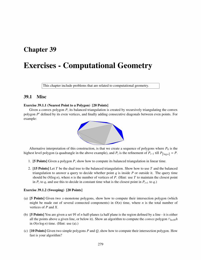
Chapter 39

Exercises - Computational Geometry

This chapter include problems that are related to computational geometry.

39.1 Misc

Exercise 39.1.1 (Nearest Point to a Polygon) [20 Points]Given a convex polygon P, its balanced triangulation is created by recursively triangulating the convex

polygon P′ defined by its even vertices, and finally adding consecutive diagonals between even points. Forexample:

Alternative interpretation of this construction, is that we create a sequence of polygons where P0 is thehighest level polygon (a quadrangle in the above example), and Pi is the refinement of Pi−1 till Pdlog ne = P.

1. [5 Points] Given a polygon P, show how to compute its balanced triangulation in linear time.

2. [15 Points] Let T be the dual tree to the balanced triangulation. Show how to use T and the balancedtriangulation to answer a query to decide whether point q is inside P or outside it. The query timeshould be O(log n), where n is the number of vertices of P. (Hint: use T to maintain the closest pointin Pi to q, and use this to decide in constant time what is the closest point in Pi+1 to q.)

Exercise 39.1.2 (Sweeping) [20 Points]

(a) [5 Points] Given two x-monotone polygons, show how to compute their intersection polygon (whichmight be made out of several connected components) in O(n) time, where n is the total number ofvertices of P and X.

(b) [5 Points] You are given a setH of n half-planes (a half plane is the region defined by a line - it is eitherall the points above a given line, or below it). Show an algorithm to compute the convex polygon ∩h∈Hhin O(n log n) time. (Hint: use (a).)

(c) [10 Points] Given two simple polygons P and Q, show how to compute their intersection polygon. Howfast is your algorithm?

279

What the maximum number of connected components of the polygon P ∩ Q (provide a tight upper andlower bounds)?

Exercise 39.1.3 (Robot Navigation) [20 Points]Given a set S of m simple polygons in the plane (called obstacles), with total complexity n, and start

point s and end point t, find the shortest path between s and t (this is the path that a robot would take tomove from s to t).

1. [5 Points] For a point q ∈ IR2, which is not contained in any of the obstacles, the visibility polygon ofq, is the set of all the points in the plane that are visible form q. Show how to compute this visibilitypolygon in O(n log n) time.

2. [5 Points] Show a O(n3) time algorithm for this problem. (Hint: Consider the shortest path, andanalyze its structure. Build an appropriate graph, and do a Dijkstra in this graph.)).

3. [10 Points] Show a O(n2 log n) time algorithm for this problem.

Exercise 39.1.4 (Point-Location) Given a x-monotone polygonal chain C with n vertices, show how topreprocess it in linear time, such that given a query point q, one can decide, in O(log n) time, whether q isbelow and above C, and what is the segment of C that intersects the vertical line that passes through q. Showhow to use this to decide, in O(log n) whether a point p is inside a x-monotone polygon P with n vertices.Why would this method be preferable to the balanced triangulation used in the previous question (when usedon a convex polygon)?

Exercise 39.1.5 (Convexity revisited.) (a) Prove that for any set S of four points in the plane, there existsa partition of S into two subsets S 1, S 2, such that CH(S 1) ∩ CH(S 2) , ∅.

(b) Prove that any point x which is a convex combination of n points p1, . . . , pn in the plane, can be definedas a convex combination of three points of p1, . . . , pn. (Hint: use (a) and induction on the number ofpoints.)

(c) Prove that for any set S of d + 2 points in IRd, there exists a partition of S into two subsets S 1, S 2, suchthat CH(S 1) ∩ CH(S 2) , ∅, S = S 1 ∪ S 2, and S 1 ∩ S 2 = ∅. (Hint: Use (a) and induction on thedimension.)

Exercise 39.1.6 (Covered by triangles) You are given a set of n triangles in the plane, show an algorithm,as fast as possible, that decides whether the square [0, 1] × [0, 1] is completely covered by the triangles.

Exercise 39.1.7 (Nearest Neighbor) Let P be a set of n points in the plane. For a point p ∈ P, its nearestneighbor in P, is the point in P \ p which has the smallest distance to p. Show how to compute for everypoint in P its nearest neighbor in O(n log n) time.

280

Chapter 40

Exercises - Entropy

Exercise 40.0.8 (Compress a sequence.) We wish to compress a sequence of independent, identically dis-tributed random variables X1, X2, , . . .. Each X j takes on one of n values. The ith value occurs with proba-bility pi, where p1 ≥ p2 ≥ . . . ≥ pn. The result is compressed as follows. Set

Ti =

i−1∑j=1

p j,

and let the ith codeword be the first⌈lg(1/pi)

⌉bits of Ti. Start with an empty string„ and consider X j in

order. If X j takes on the ith value, append the ith codeword to the end of the string.

(A) Show that no codeword is the prefix of any other codeword.

(B) Let Z be the average number of bits appended for each random variable X j. Show that

H(X j

)≤ z ≤ H

(X j

)+ 1.

Exercise 40.0.9 (Arithmetic coding) Arithmetic coding is a standard compression method. In the casewhen the string to be compressed is a sequence of biased coin flips, it can be described as follows. Supposethat we have a sequence of bits X = (X1, X2, . . . , Xn), where each Xi is independently 0 with probability pand 1 with probability 1 − p. The sequences can be ordered lexicographically, so for x = (x1, x2, . . . , xn andy = (y1, y2, . . . , yn), we say that x < y if xi = 0 and yi = 1 in the first coordinate i such that xi , yi. If z(x) isthe nubmer of zeroes in the string x, then define p(x) = pz(x)(1 − p)n−z(x) and

q(x) =∑y<x

p(y).

(A) Suppose we are given X = (X1, X2, . . . , Xn). Explain how to compute q(X) in time O(n) (assume thatany reasonable operation on real numbers takes constant time).

(B) Argue that the intervals[q(x), q(x) + p(x)

)are disjoint subintervals of [0, 1).

(C) Given (A) and (B), the sequence X can be represented by any point in the interval I(X) =[q(X), q(X) + p(X)

).

Show that we can choose a codeword in I(X) with⌈lg(1/p(X))

⌉+ 1 binary decimal digits to represent

X in such a way that no codeword is the prefix of any other codeword.

(D) Given a codeword chosen as in (C), explain how to decompress it to determine the correspondingsequence (X1, X2, . . . , Xn).

281

(E) Using the Chernoff inequality, argue that lg(1/p(X)) is close to nH (p) with high probability. Thus, thisapproach yields an effective compression scheme.

Exercise 40.0.10 (Computing entropy.) 1. Let S =∑10

i=1 1/i2. Consider a random variable X such thatPr[X = i] = 1/(S i2), for i = 1, . . . , 10. Compute H (X).

2. Let S =∑10

i=1 1/i3. Consider a random variable X such that Pr[X = i] = 1/(S i3), for i = 1, . . . , 10.Compute H (X).

3. Let S (α) =∑10

i=1 1/iα, for α > 1. Consider a random variable X such that Pr[X = i] = 1/(S (α)iα), fori = 1, . . . , 10. Prove that H (X) is either increasing or decreasing as a function of α (you can assumethat α is an integer).

Exercise 40.0.11 (When is entropy maximized?) Consider an n-sided die, where the ith face comes upwith probability pi. Show that the entropy of a die roll is maximized when each face comes up with equalprobability 1/n.

Exercise 40.0.12 (Condition entropy.) The conditional entropy H (Y |X) is defined by

H(Y |X) =∑x,y

Pr[(X = x) ∩ (Y = y)

]lg

1Pr

[Y = y|X = x

] .If Z = (X,Y), prove that

H (Z) = H (X) + H (Y |X) .

Exercise 40.0.13 (Improved randomness extraction.) We have shown that we can extract, on average, atleast

⌊lg m

⌋− 1 independent, unbiased bits from a number chosen uniformly at random from 0, . . . ,m − 1.

It follows that if we have k numbers chosen independently and uniformly at random from 0, . . . ,m − 1then we can extract, on average, at least k

⌊lg m

⌋− k independent, unbiased bits from them. Give a better

procedure that extracts, on average, at least k⌊lg m

⌋− 1 independent, unbiased bits from these numbers.

Exercise 40.0.14 (Kraft inequality.)

Assume you have a (valid) prefix code with n codewords, where the ith codeword is made out of `i bits.Prove that

n∑i=1

12li≤ 1.

282

Bibliography

[ACG+99] G. Ausiello, P. Crescenzi, G. Gambosi, V. Kann, A. Marchetti-Spaccamela, and M. Protasi.Complexity and approximation. Berlin, 1999.

[AKS83] M. Ajtai, J. Komlós, and E. Szemerédi. An O(n log n) sorting network. In Proc. 15th Annu.ACM Sympos. Theory Comput., pages 1–9, 1983.

[AN04] N. Alon and A. Naor. Approximating the cut-norm via grothendieck’s inequality. In Proc. 36thAnnu. ACM Sympos. Theory Comput., pages 72–80, 2004.

[ASS96] H. Abelson, G. J. Sussman, and J. Sussman. Structure and interpretation of computer pro-grams. MIT Press, 1996.

[BV04] S. Boyd and L. Vandenberghe. Convex Optimization. Cambridge, 2004.

[Chr76] N. Christofides. Worst-case analysis of a new heuristic for the travelling salesman problem.Technical Report Report 388, Graduate School of Industrial Administration, Carnegie MellonUniversity, 1976.

[FG88] T. Feder and D. H. Greene. Optimal algorithms for approximate clustering. In Proc. 20th Annu.ACM Sympos. Theory Comput., pages 434–444, 1988.

[FG95] U. Feige and M. Goemans. Approximating the value of two power proof systems, with appli-cations to max 2sat and max dicut. In ISTCS ’95: Proceedings of the 3rd Israel Symposium onthe Theory of Computing Systems (ISTCS’95), page 182, Washington, DC, USA, 1995. IEEEComputer Society.

[GJ90] M. R. Garey and D. S. Johnson. Computers and Intractability; A Guide to the Theory of NP-Completeness. W. H. Freeman & Co., New York, NY, USA, 1990.

[GLS88] M. Grötschel, L. Lovász, and A. Schrijver. Geometric Algorithms and Combinatorial Opti-mization, volume 2 of Algorithms and Combinatorics. Springer-Verlag, Berlin Heidelberg,2nd edition, 1988. 2nd edition 1994.

[GT89] A. V. Goldberg and R. E. Tarjan. Finding minimum-cost circulations by canceling negativecycles. J. Assoc. Comput. Mach., 36(4):873–886, 1989.

[GW95] M. X. Goemans and D. P. Williamson. Improved approximation algorithms for maximumcut and satisfiability problems using semidefinite programming. J. Assoc. Comput. Mach.,42(6):1115–1145, November 1995.

[Har04] S. Har-Peled. Clustering motion. Discrete Comput. Geom., 31(4):545–565, 2004.

283

http://www.math.tau.ac.il/~nogaa/

http://www.acm.org/jacm/


http://www.uiuc.edu/~sariel

http://link.springer-ny.com/link/service/journals/00454/

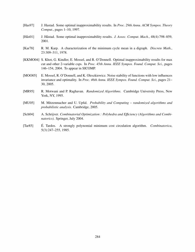
[Has97] J. Hastad. Some optimal inapproximability results. In Proc. 29th Annu. ACM Sympos. TheoryComput., pages 1–10, 1997.

[Hås01] J. Håstad. Some optimal inapproximability results. J. Assoc. Comput. Mach., 48(4):798–859,2001.

[Kar78] R. M. Karp. A characterization of the minimum cycle mean in a digraph. Discrete Math.,23:309–311, 1978.

[KKMO04] S. Khot, G. Kindler, E. Mossel, and R. O’Donnell. Optimal inapproximability results for maxcut and other 2-variable csps. In Proc. 45th Annu. IEEE Sympos. Found. Comput. Sci., pages146–154, 2004. To appear in SICOMP.

[MOO05] E. Mossel, R. O’Donnell, and K. Oleszkiewicz. Noise stability of functions with low influencesinvariance and optimality. In Proc. 46th Annu. IEEE Sympos. Found. Comput. Sci., pages 21–30, 2005.

[MR95] R. Motwani and P. Raghavan. Randomized Algorithms. Cambridge University Press, NewYork, NY, 1995.

[MU05] M. Mitzenmacher and U. Upfal. Probability and Computing – randomized algorithms andprobabilistic analysis. Cambridge, 2005.

[Sch04] A. Schrijver. Combinatorial Optimization : Polyhedra and Efficiency (Algorithms and Combi-natorics). Springer, July 2004.

[Tar85] É. Tardos. A strongly polynomial minimum cost circulation algorithm. Combinatorica,5(3):247–255, 1985.

284




Index

(k, n) decoding function, 195(k, n) encoding function, 1950/1-flow, 95

algorithmrandomized, 51

alternating BFS, 207alternating cycle, 204alternating path, 204approximation

algorithmminimization, 46

maximization problem, 51Arithmetic coding, 281augmenting path, 88

Bin Packingnext fit, 61

bin packingfirst fit, 62

binary code, 181binary symmetric channel, 195bitonic sequence, 140Bland’s rule, 155blossom, 208

capacity, 85, 89Chernoff inequality, 71Cholesky decomposition, 169circulation, 97clique, 21clustering

k-center, 56price, 56

code trees, 181coloring, 24comparison network, 138

depth, 138depth wire, 138

half-cleaner, 140sorting network, 138

conditional entropy, 282conditional probability, 75congestion, 162contraction

edge, 76convex, 40convex polygon, 40cut, 75, 89

minimum, 75cuts, 75Cycle

directed, 111Eulerian, 48

DAG, 138decision problem, 16diagonal, 40digraph, 111directed, 85directed cut, 89directed Cycle

average cost, 111disjoint paths

edge, 95distance

point from set, 55

edge disjointpaths, 95

edit distance, 36entering, 154entropy, 185, 187

binary, 187Eulerian cycle, 27, 48expectation

linearity, 65

285

facility location problem, 55Fast Fourier Transform, 130feasible, 105fixed parameter tractable, 247Flow

capacity, 85Integrality theorem, 92value, 86

flow, 85, 860/1-flow, 95circulation

minimum-cost, 114valid, 114

cost, 113efficient, 123min cost

reduced cost, 117minimum-cost, 114residual graph, 87residual network, 87

flow network, 85flower, 208flow

flow across a cut, 89Ford-Fulkerson method, 89FPTAS, 59fully polynomial time approximation scheme, 59

gadget, 24greedy algorithms, 45

Hamiltonian cycle, 27high probability, 67Huffman coding, 183

i, 156image segmentation problem, 103independent, 75independent set, 23induced subgraph, 21

leader, 217leaving, 154Linear programming

standard form, 146linear programming, 145

constraint, 145dual, 155dual program, 157

entering variable, 154pivoting, 149primal, 155primal problem, 156primal program, 157slack form, 147slack variable, 147variable

basic, 147non-basic, 147

Linearity of expectations, 51longest ascending subsequence, 42lucky, 70

Macaroni sort, 137Markov’s Inequality, 70matching, 49, 93

bridge, 207free edge, 204free vertex, 204matching edge, 204maximum matching, 93perfect, 49, 93

maximum cut problem, 167maximum flow, 86memoization, 34merge sort, 142min-weight perfect matching, 49mincut, 75minimum average cost cycle, 111minimum cut, 89

network, 85

objective function, 145

partition number, 33path

augmenting, 204pivoting, 154point-value pairs, 129polynomial, 129polynomial reductions, 18polynomial time approximation scheme, 59positive semidefinite, 169potential, 113prefix code, 181prefix-free, 181probabilistic method, 199

286

ProbabilityAmplification, 78

probability, 161conditional, 65

Problemk-CENTER, 2442SAT, 54, 239

2SAT Max, 543CNF, 293COLORABLE, 2453Colorable, 24, 253DM, 303SAT, 19, 20, 22, 24, 29, 30, 51, 239

2SAT Max, 543SAT Max, 51, 54

A, 21AFWLB, 123, 124BIN PACKING, 238, 241, 243Bin Packing, 61bin packing

min, 61Circuit Satisfiability, 16–19Clique, 23clustering

k-center, 56CSAT, 18–20EXACT-COVER-BY-3-SETS, 239formula satisfiability, 17, 19Hamiltonian Cycle, 27, 47Hamiltonian Path, 124, 240Hamiltonian path, 124HITTING SET, 239–241, 244Independent Set, 23, 24, 247Integer Linear Programming, 276KNAPSACK, 242LARGEST COMMON SUBGRAPH, 238Max 3SAT, 51MAX CUT, 167Max Degree Spanning Tree, 240MAX SAT, 244MaxClique, 21, 22MINIMUM SET COVER, 238, 240, 241, 243Minimum Test Collection, 237MULTIPROCESSOR SCHEDULING, 242Not-3SAT, 240NPC, 29PARTITION, 241Partition, 30, 31, 61, 237, 238

PRIMALITY, 246PROB, 59reduction, 237SAT, 17–19Set Cover, 46, 53, 161Sorting Nuts and Bolts, 66SUBGRAPH ISOMORPHISM, 238Subgraph Isomorphism, 237SUBSET SUM, 241Subset Sum, 29–31, 58, 59, 239subset sum

approximation, 58optimization, 58

TILING, 238, 242, 243TSP, 28, 47, 48

Min, 47With the triangle inequality, 48

Vec Subset Sum, 29, 31VERTEX COVER, 242Vertex Cover, 24, 27, 28, 45, 159, 247, 267

Min, 45–47Minimization, 45

VertexCover, 46, 267Weighted Vertex Cover, 159, 160X, 21, 22

problemminimization, 45

profit, 105PTAS, 59

random variable, 65random variables

independent, 65rank, 66relaxation, 160residual capacity, 87, 88residual graph, 114rounding, 160running-time

amortized, 215expected, 66

see, 52shortcutting, 48sink, 85slack form, 147sorting network

bitonic sorter, 140

287

running time, 138size, 138zero-one principle, 139

source, 85stem, 208, 209

transportation problem, 125tree

prefix tree, 181triangle inequality, 48

union rule, 69union-find

block of a node, 219jump, 220

internal, 220path compression, 216rank, 216union by rank, 216

unsupervised learning, 55

value, 86Vandermonde, 132vertex cover, 23visibility polygon, 53

weak circulation, 114weight

cycle, 204

288

Algorithms Book

Documents

player p0 names

longest ascending subsequence

creative commons attribution

breaking ties arbitrarily

x2 y2

separation penalty pi

dynamic programming ii

vertexdisjoint augmenting paths