Agarwal a Phd

Authoring effective depictions of reality by combining multiple samples ofthe plenoptic function

Aseem Agarwala

A dissertation submitted in partial fulfillmentof the requirements for the degree of

Doctor of Philosophy

University of Washington

2006

Program Authorized to Offer Degree: Computer Science & Engineering

University of WashingtonGraduate School

This is to certify that I have examined this copy of a doctoral dissertation by

Aseem Agarwala

and have found that it is complete and satisfactory in all respects,and that any and all revisions required by the final

examining committee have been made.

Chair of the Supervisory Committee:

David H. Salesin

Reading Committee:

David H. Salesin

Steven M. Seitz

Michael H. Cohen

Date:

In presenting this dissertation in partial fulfillment of the requirements for the doctoral degree atthe University of Washington, I agree that the Library shall make its copies freely available forinspection. I further agree that extensive copying of this dissertation is allowable only for scholarlypurposes, consistent with “fair use” as prescribed in the U.S. Copyright Law. Requests for copyingor reproduction of this dissertation may be referred to Proquest Information and Learning, 300North Zeeb Road, Ann Arbor, MI 48106-1346, 1-800-521-0600, to whom the author has granted“the right to reproduce and sell (a) copies of the manuscript in microform and/or (b) printed copiesof the manuscript made from microform.”

Signature

Date

University of Washington

Abstract

Authoring effective depictions of reality by combining multiple samples of the plenopticfunction

Aseem Agarwala

Chair of the Supervisory Committee:

Professor David H. Salesin

Computer Science & Engineering

Cameras are powerful tools for depicting of the world around us, but the images they produce

are interpretations of reality that often fail to resemble our intended interpretation. The recent digiti-

zation of photography and video offers the opportunity to move beyond the traditional constraints of

analog photography and improve the processes by which light in a scene is mapped into a depiction.

In this thesis, I explore one approach to addressing this challenge. My approach begins by capturing

multiple digital photographs and videos of a scene. I present algorithms and interfaces that identify

the best pieces of this captured imagery, as well as algorithms for seamlessly fusing these pieces

into new depictions that are better than any of the originals. As I show in this thesis, the results are

often much more effective than what could be achieved using traditional techniques.

I apply this approach to three projects in particular. The ”photomontage” system is an interac-

tive tool that partially automates the process of combining the best features of a stack of images.

The interface encourages the user to consider the input stack of images as a single entity, pieces

of which exhibit the user’s desired interpretation of the scene. The user authors a composite image

(photomontage) from the input stack by specifying high-level objectives it should exhibit, either

globally or locally through a painting interface. I describe an algorithm that then constructs a depic-

tion from pieces of the input images by maximizing the user-specified objectives while also mini-

mizing visual artifacts. In the next project, I extend the photomontage approach to handle sequences

of photographs captured from shifted viewpoints. The output is a multi-viewpoint panorama that

is particularly useful for depicting scenes too long to effectively image with the single-viewpoint

perspective of a traditional camera. In the final project, I extend my approach to video sequences.

I introduce the “panoramic video texture”, which is a video with a wide field of view that appears

to play continuously and indefinitely. The result is a new medium that combines the benefits of

panoramic photography and video to provide a more immersive depiction of a scene. The key chal-

lenge in this project is that panoramic video textures are created from the input of a single video

camera that slowly pans across the scene; thus, although only a portion of the scene has been imaged

at any given time, the output must simultaneously portray motion throughout the scene. Throughout

this thesis, I demonstrate how these novel techniques can be used to create expressive visual media

that effectively depicts the world around us.

TABLE OF CONTENTS

List of Figures . . . . . . . . . . . . . . . . . . . . . . . . . . . . . . . . . . . . . . . . . . iii

Chapter 1: Introduction . . . . . . . . . . . . . . . . . . . . . . . . . . . . . . . . . . 1

1.1 Parameterizing light . . . . . . . . . . . . . . . . . . . . . . . . . . . . . . . . . . 3

1.2 Interpreting light . . . . . . . . . . . . . . . . . . . . . . . . . . . . . . . . . . . 4

Chapter 2: A framework . . . . . . . . . . . . . . . . . . . . . . . . . . . . . . . . . 11

2.1 My approach . . . . . . . . . . . . . . . . . . . . . . . . . . . . . . . . . . . . . 12

2.2 Previous work . . . . . . . . . . . . . . . . . . . . . . . . . . . . . . . . . . . . . 15

Chapter 3: Interactive digital photomontage . . . . . . . . . . . . . . . . . . . . . . . 28

3.1 Introduction . . . . . . . . . . . . . . . . . . . . . . . . . . . . . . . . . . . . . . 28

3.2 The photomontage framework . . . . . . . . . . . . . . . . . . . . . . . . . . . . 34

3.3 Graph cut optimization . . . . . . . . . . . . . . . . . . . . . . . . . . . . . . . . 37

3.4 Gradient-domain fusion . . . . . . . . . . . . . . . . . . . . . . . . . . . . . . . . 39

3.5 Results . . . . . . . . . . . . . . . . . . . . . . . . . . . . . . . . . . . . . . . . . 41

3.6 Conclusions and future work . . . . . . . . . . . . . . . . . . . . . . . . . . . . . 48

Chapter 4: Photographing long scenes with multi-viewpoint panoramas . . . . . . . . 54

4.1 System details . . . . . . . . . . . . . . . . . . . . . . . . . . . . . . . . . . . . . 60

4.2 Results . . . . . . . . . . . . . . . . . . . . . . . . . . . . . . . . . . . . . . . . . 70

4.3 Future work . . . . . . . . . . . . . . . . . . . . . . . . . . . . . . . . . . . . . . 72

Chapter 5: Panoramic video textures . . . . . . . . . . . . . . . . . . . . . . . . . . . 77

5.1 Introduction . . . . . . . . . . . . . . . . . . . . . . . . . . . . . . . . . . . . . . 77

5.2 Problem definition . . . . . . . . . . . . . . . . . . . . . . . . . . . . . . . . . . 79

5.3 Our approach . . . . . . . . . . . . . . . . . . . . . . . . . . . . . . . . . . . . . 84

5.4 Gradient-domain compositing . . . . . . . . . . . . . . . . . . . . . . . . . . . . 89

5.5 Results . . . . . . . . . . . . . . . . . . . . . . . . . . . . . . . . . . . . . . . . . 94

5.6 Limitations . . . . . . . . . . . . . . . . . . . . . . . . . . . . . . . . . . . . . . 95

5.7 Future work . . . . . . . . . . . . . . . . . . . . . . . . . . . . . . . . . . . . . . 96

i

5.8 Conclusion . . . . . . . . . . . . . . . . . . . . . . . . . . . . . . . . . . . . . . 97

Chapter 6: Conclusion . . . . . . . . . . . . . . . . . . . . . . . . . . . . . . . . . . 98

6.1 Contributions . . . . . . . . . . . . . . . . . . . . . . . . . . . . . . . . . . . . . 98

6.2 Future work . . . . . . . . . . . . . . . . . . . . . . . . . . . . . . . . . . . . . . 99

Bibliography . . . . . . . . . . . . . . . . . . . . . . . . . . . . . . . . . . . . . . . . . . 103

ii

LIST OF FIGURES

Figure Number Page

1.1 Demonstrations of constancy . . . . . . . . . . . . . . . . . . . . . . . . . . . . . 8

1.2 “The School of Athens” by Raphael (1509) . . . . . . . . . . . . . . . . . . . . . 9

2.1 Framework diagram . . . . . . . . . . . . . . . . . . . . . . . . . . . . . . . . . . 11

2.2 An example composite depiction . . . . . . . . . . . . . . . . . . . . . . . . . . . 13

2.3 Two inspirational photographs . . . . . . . . . . . . . . . . . . . . . . . . . . . . 21

2.4 Multi-perspective artwork by Michael Koller . . . . . . . . . . . . . . . . . . . . 23

3.1 A flow diagram of a typical interaction with my photomontage framework . . . . . 33

3.2 Family portait photomontage . . . . . . . . . . . . . . . . . . . . . . . . . . . . . 42

3.3 Individual portait photomontage . . . . . . . . . . . . . . . . . . . . . . . . . . . 42

3.4 Composite portait photomontage . . . . . . . . . . . . . . . . . . . . . . . . . . . 43

3.5 Family portait photomontage of famous researchers . . . . . . . . . . . . . . . . . 44

3.6 Face relighting photomontage . . . . . . . . . . . . . . . . . . . . . . . . . . . . 45

3.7 Bronze sculpture photomontage . . . . . . . . . . . . . . . . . . . . . . . . . . . 46

3.8 Extended depth of field photomontage . . . . . . . . . . . . . . . . . . . . . . . . 47

3.9 Panoramic photomontage . . . . . . . . . . . . . . . . . . . . . . . . . . . . . . . 49

3.10 Background reconstruction photomontage . . . . . . . . . . . . . . . . . . . . . . 50

3.11 Wire removal photomontage . . . . . . . . . . . . . . . . . . . . . . . . . . . . . 50

3.12 Stroboscopic photomontage . . . . . . . . . . . . . . . . . . . . . . . . . . . . . . 51

3.13 Timelapse photomontage . . . . . . . . . . . . . . . . . . . . . . . . . . . . . . . 52

4.1 Multi-viewpoint panorama of Antwerp street . . . . . . . . . . . . . . . . . . . . 55

4.2 Hypothetical scene plan view . . . . . . . . . . . . . . . . . . . . . . . . . . . . . 59

4.3 Multi-viewpoint panorama system overview . . . . . . . . . . . . . . . . . . . . . 59

4.4 Plan view . . . . . . . . . . . . . . . . . . . . . . . . . . . . . . . . . . . . . . . 63

4.5 River bank plan view . . . . . . . . . . . . . . . . . . . . . . . . . . . . . . . . . 63

4.6 Projected source image . . . . . . . . . . . . . . . . . . . . . . . . . . . . . . . . 64

4.7 Average projected image, cropped and unwarped . . . . . . . . . . . . . . . . . . 64

4.8 Seams and sources for Antwerp street panorama . . . . . . . . . . . . . . . . . . . 65

iii

4.9 Multi-viewpoint panorama of Antwerp street . . . . . . . . . . . . . . . . . . . . 71

4.10 Longest multi-viewpoint panorama of Antwerp street . . . . . . . . . . . . . . . . 74

4.11 Multi-viewpoint panorama of a grocery store aisle . . . . . . . . . . . . . . . . . . 74

4.12 Multi-viewpoint panorama of Charleston street . . . . . . . . . . . . . . . . . . . 75

4.13 Multi-viewpoint panorama of a riverbank . . . . . . . . . . . . . . . . . . . . . . 76

5.1 One frame of the waterfall panoramic video texture. . . . . . . . . . . . . . . . 78

5.2 Constructing a PVT . . . . . . . . . . . . . . . . . . . . . . . . . . . . . . . . . . 80

5.3 Naive approach to constructing a PVT . . . . . . . . . . . . . . . . . . . . . . . . 81

5.4 Comparison of results for two approaches to constructing PVTs . . . . . . . . . . 82

5.5 Constrained formulation solution . . . . . . . . . . . . . . . . . . . . . . . . . . . 86

5.6 One frame of three PVTs . . . . . . . . . . . . . . . . . . . . . . . . . . . . . . . 91

5.7 An x, t slice of the constrained formulation result for waterfall PVT . . . . . . . 92

5.8 An x, t slice of the final result for waterfall PVT . . . . . . . . . . . . . . . . . 93

iv

ACKNOWLEDGMENTS

I would like to first thank my numerous collaborators for the projects described in chapters 3-

5, which include Professors David Salesin, Brian Curless, and Maneesh Agrawala, UW students

Mira Dontcheva and Colin Zheng, and Microsoft Research collaborators Michael Cohen, Richard

Szeliski, Chris Pal, Alex Colburn, and Steven Drucker. For the two projects I completed during my

time at UW that were not included as chapters in this thesis [28, 4], my collaborators were Yung-Yu

Chuang, Aaron Hertzmann, and Steven Seitz.

Numerous people beyond the author lists of my papers helped me immeasurably. John Longino

at Evergreen College provided the insect dataset (Figure 3.8) and feedback on the result. Vladimir

Kolmogorov authored the graph cut software used throughout this thesis. Noah Snavely wrote the

structure-from-motion system used in chapter 4. Wilmot Li created three of the figures in chapter 5,

and Drew Steedly aided with video alignment.

I would like to thank the numerous people in the graphics community that I have had the chance

to work with before coming to UW, and who helped inspire me to pursue this career, including

Matthew Brand, Carol Strohecker, Joe Marks, Julie Dorsey, and Leonard McMillan.

Finally, I would like to thank my family, and my wife Elke Van de Velde, who as a photographer

helped me to capture many of the datasets used in this thesis.

v

1

Chapter 1

INTRODUCTION

Photographs are as much an interpretation of the world as paintings and drawings are.

– Susan Sontag [130]

A depiction is any sort of visual representation of a scene. We create depictions in many forms,

and for many purposes. The mediums of depiction include photography, video, paintings, line draw-

ings, and the rendering of three-dimensional models. The compulsion to portray the visual world

seems innate, as evidenced by the long history of depiction which extends from primitive cave

paintings to the introduction of the rules of perspective in the 1400’s [76]. The invention of the

Daguerrotype in the 1830’s [100] caused an immediate sensation, because it allowed those with no

skill in painting to create images that conveyed an incredibly powerful illusion of reality. In modern

times, photography (for convenience, I will include both still and moving images under the umbrella

of photography) has become our most frequently-used tool for visual communication. Images of all

kinds constantly bombard us with information about the world: advertisements, magazine illustra-

tions, television, and even postage stamps and driver’s licenses.

We create photographic depictions of reality for many reasons. Perhaps the most common mo-

tivation can be found in our snapshots and home movies that we create to embody our visual mem-

ories – to capture an impression of reality that will remind of past locations and events, keep our

memories fresh, and trigger vivid recollections. We also use photographs as visual messages, such

as advertising that encourages you to purchase, or films that entertain you with an imaginary reality.

Cameras play a crucial role in more utilitarian pursuits. Among other things, photographs and video

document the appearance of archaeological specimens, medical ailments, real estate, and tourist

destinations.

Photographs provide a powerful illusion of reality, but it is important to remember that pho-

2

tographs are not “real”; they are interpretations of reality with many degrees of freedom in their

construction. Traditional cameras map captured light into images in a limited and specific fashion,

and the depictions they produce may not be effective at expressing what the authors hope to com-

municate. For example, many personal snapshots are marred by motion blur and poor lighting, and

don’t look much like what we remember when we experienced the scene with our own eyes.

The recent digitization of photography offers an unprecedented opportunity for computer scien-

tists to rethink the processes by which we create depictions of reality, and to move beyond traditional

photographic techniques to create depictions that communicate more effectively. The tools at our

disposal include digital sensors that capture light in the world, and computational algorithms that

can model and manipulate digitized light. The challenge at hand, then, is to develop novel devices

and software that map from light in a scene to powerful and expressive visual communication that

is easy for a user to create.

In this thesis, I explore one approach to addressing this challenge. My approach begins by cap-

turing multiple samples of light in the world, in the form of multiple digital photographs and videos.

I then develop algorithms and interfaces that identify the best pieces of these multiple samples, as

well as algorithms for fusing these pieces into new depictions that are better than any of the original

samples. As I show in this thesis, the results are often much more powerful than what could be

achieved using traditional techniques.

In the rest of this chapter, I will first describe how to parameterize all of the light that exists

in a scene. I will then use this parameterization to describe how cameras sample light to create

depictions, and how humans sample light during visual consciousness. Finally, I will re-enforce the

notion that both photographs and human visual consciousness are mere interpretations of reality,

and that they represent very different ways to interpret the light in a scene. These differences will

make clear the many degrees of freedom in interpreting light that can be exploited to create better

depictions. In the subsequent chapter I will describe an overall framework for techniques that create

better depictions by combining multiple samples of the light in a scene, as well as related work and

an overview of my own research and contributions within the context of this framework.

Chapters 3- 5 will give technical details and results for each of the three projects that form the

bulk of this thesis. Finally, I will conclude this thesis by summarizing my contributions and offering

ideas for future work.

3

1.1 Parameterizing light

We see reality through light that reflects from objects in our environment. This light can be modeled

as rays that travel through three-dimensional space without interfering with each other. Imagine

a parameterized function of all the rays of light that exist throughout three-dimensional space and

time, which describes the entire visual world and contains enough information to create any possible

photograph or video ever taken. Adelson and Bergen [1] showed that this function, which they call

the plenoptic function, can be parameterized by seven parameters: a three-dimensional location in

space (Vx, Vy, Vz), time (t), the wavelength of the light (λ ), and the direction of the light passing

through the location (parameterized by spherical coordinates θ ,φ ). Given these seven parameters,

the plenoptic function returns the intensity of light (radiance). Thus, the plenoptic function provides

a precise notion of the visual world surrounding us that we wish to depict.

1.1.1 Photographing light

The etymology of the word “photography” arises from the Greek words phos (“light”) and graphis

(“stylus”); together, the term can be literally translated as “drawing with light.”

The first step in “drawing with light” is to sample the light in a scene. Any photograph or video

is thus formed by sampling the plenoptic function, and it is useful to understand the nature of this

sampling. An ideal camera obscura with an infinitely small pinhole will select a pencil1 of rays and

project a subset of them onto a two-dimensional surface to create an image. Assuming the surface

is a black and white photosensitive film, the final image will provide samples of radiance along a

certain interval over two axes of the plenoptic function: x and y (the interval depends on the size

of the film, and the sampling rate depends on the size of the film grain). The pinhole location Vx,

Vy, Vz is fixed, and variations over a short range of time and wavelength are integrated into one

intensity. The film will only have a certain dynamic range; that is, if the intensity returned by the

plenoptic function is too great or too small, it will be clipped to the limits of the film. Also, films

(and digital sensors) are not perfect at recording light, and thus will exhibit noise; film has a signal-

to-noise ratio that expresses how grainy the output will be given a certain amount of incoming light.

Typically, increasing the light that impinges on the film will increase the signal-to-noise ratio. A

1The set of rays passing through any single point is referred to as a pencil.

4

360o panorama extends the sampling of a photograph to cover all directions of light θ ,φ . Color film

samples across a range of wavelengths. A video from a stationary camera samples over a range of

time. Stereoscopic and holographic images also sample along additional parameters of the plenoptic

function. Note, however, that modern cameras do not operate like ideal pinholes. An ideal pinhole

camera has an infinitely small aperture, which in a practical setting would not allow enough light

to reach the film plane to form an image. Instead, cameras use a lens to capture and focus a wider

range of rays. Thus, modern cameras do not interpret a pencil of light rays, but a subset of the rays

impinging upon its lens.

1.1.2 Seeing light

The human eye can be thought of as an optical device similar to a camera; light travels through a pin-

hole (iris) and projects onto a two-dimensional surface. The light stimulates sensors (cones) on this

surface, and signals from these sensors are then transmitted to the brain. Human eyes can sample the

plenoptic function simultaneously along five axes. Our two eyes provide two samples along a single

spatial dimension (Vx) over a range of time. Information along the wavelength axis is extracted using

three types of cones, which respond to a much larger dynamic range than film or digital sensors. Our

eyes adjust dynamically to illumination conditions, in a process called adaption. Finally, we sample

along a range of incoming directions x,y (though the resolution of that sampling varies spatially).

We fuse our interpretation of these samples across five dimensions into the depiction we see in our

mind’s eye.

1.2 Interpreting light

I have shown that human vision and cameras sample the plenoptic function differently; in this sec-

tion, I show that they also interpret light in drastically different fashions. In this thesis I explore a

computational approach to interpreting light captured by a camera in order to create better depic-

tions; to understand my approach it is first useful to understand how both traditional cameras and

humans interpret light, and the differences between them.

Once light in the world is sampled in some fashion, this light must be processed and interpreted

into an understandable form. Digital cameras convert sampled light into digital signals, and then

5

further process those signals into images that can be printed or viewed on a display. This processing

can be controlled by a human both by adjusting parameters of the camera before capture and by

manipulating images on a computer after capture. Humans, on the other hand, convert sampled light

into neural signals that are then processed by our brains in real-time to create what we experience

during visual consciousness.

1.2.1 Photographic interpretation of light

A photographer is not simply a passive observer; he or she must make a complex set of inter-related

choices that affect the brightness, contrast, depth of field, framing, noise, and other aspects of the

final image.2 Different choices lead to very different samplings and interpretations of the plenoptic

function.

The most obvious choice a photographer must make is framing. The selection of a photograph’s

frame is an act of visual editing, which decides for the viewer which rectangular portion of the

scene he/she can see. In terms of the plenoptic function, framing a photograph involves choosing

a viewpoint Vx, Vy,Vz, and the range of directions θ ,φ that the field of view will cover (which

can be adjusted by zooming). This framing is distinct from the human eye, which has its highest

visual acuity at the center of vision and degrades quickly towards the periphery [106]. The sharp

discontinuity introduced by the frame, referred to by Sontag as the “photographic dismemberment

of reality” [130], is very different from what humans see.

The next most obvious choice is timing; a photograph captures a very thin slice of time, and

the photographer must choose which slice. Henri Cartier-Bresson refers to this slice of time as

the “decisive moment” [26], which he describes as “the simultaneous recognition, in a fraction

of a second, of the significance of an event as well as the precise organization of forms which

gives that event its proper expression.” These frozen moments often appear very different from our

phenomenological experience of a scene. For example, while a photograph might show a friend with

his eyes closed, we don’t seem to consciously notice him blinking. We tend to remember people’s

canonical facial expressions, such as a smile or a serious expression, rather than the transitions

2In contrast, when most of us take snapshots, we simply let the automatic camera determine most of the parametersand whether or not to flash. We simply hope that the result matches what we visually perceived at the moment, and thishope is often not satisfied.

6

between them. Thus, the awkward, frozen expressions in a photograph which fails to capture the

decisive moment can be very surprising.

There are many other knobs a photographer can twist to achieve different interpretations of

reality. A consequence of using lenses is limited depth of field. Objects at a certain distance from

the camera are depicted in perfect focus; the further away an object is from this ideal distance,

the less sharp its depiction. The photographer can choose this ideal distance by focusing. Depth

of field describes the range of depths, centered at this ideal distance, that will be depicted sharply.

Photographs with a large depth of field show a wider range of depths in focus. The depth of field

can be controlled in several ways, but most commonly by choosing the size of the aperture. The

photographer can also choose how much light is allowed to hit the film plane, either by adjusting

aperture, shutter speed, or by attaching lens filters. The more light the photographer allows, the less

noisy the image (as long as the light does not overwhelm the upper limits of the film’s dynamic

range). However, increasing the aperture reduces depth of field, and increased exposure time can

introduce motion blur if the scene contains motion. Finally, the brightness of a point in the image as

a function of the light impinging on that point in the film is called the radiometric response function,

and is generally complicated and non-linear [53]. The choice of film determines this function; for

digital cameras, the function can be chosen and calculated by software after the photograph is taken.

By choosing shutter speed, aperture, and film, the photographer chooses the range of incoming

radiances to depict in the image, and how that range maps to brightness. This selected range is

typically much smaller than what the human eye can see. Finally, beyond simply interpreting the

light coming into the camera, many photographers choose to actively alter it; for example, by using

flash to add light to the scene.

A photographer exploits these degrees of freedom to create his or her desired interpretation of

the light in a scene. For example, an artist can exploit limited depth of field to draw attention to

important elements in a scene (such as a product being advertised), and abstract away unnecessary

details through blur. Framing and zooming can bring our visual attention to details of our world that

we would normally ignore. Long shutter times may blur motion unrealistically, but can be used to

suggest motion in an otherwise static medium. Limited dynamic range can be used to accentuate

contrast or hide detail in unimportant areas.

7

1.2.2 Human interpretation of light

The human visual system also constructs an interpretation of the light in scene, but one very different

from photography and video. As already described, humans sample the plenoptic function much

more widely than a camera in order to construct visual consciousness; however, this fairly complex

construction process is, for the most part, unconscious. Our brain receives two distinct sets of signals

from two eyes, yet our mind’s eye seems to depict the world as a single entity. This integration of

two signals into one is called binocular fusion. Beyond this, our eyes are constantly moving. These

motions include large-scale movements, which we consciously direct, as well as constant, small-

scale movements called saccades [106]. These movements also slightly change the viewpoint Vx,

Vy, Vz, since we move our head when looking in different directions, even when we think we’re

not [20]. In fact, subjects told to keep their heads still and eyes fixed still show appreciable amounts

of saccades and head movements [131]. This constant shifting means that the signals traveling from

the eyes to our brain are constantly changing; yet, despite this constant motion we perceive a stable

world; understanding this perceptual stability is one of the great challenges of vision science [20,

106]. Even more surprising are experiments that compensate for saccades and project an unmoving

image on the eye (this can be done with a tiny projector attached to a contact lens worn by the

subject [106]). Within a few seconds, the pattern disappears! It seems that this constant movement

is central to how we see the world.

These observations have led perception researchers to believe that we construct our visual con-

sciousness over time [105], even for a static scene. We move our two eyes over the scene, fixating on

different parts, and construct one, grand illusion of reality that is our subjective impression. Further

evidence for this theory is provided by the large blind spot in the center of our vision field where

the optic nerve meets the back of the eye. Our brain fills-in this blind spot when constructing visual

consciousness. Also, like any lens, our eyes have a limited depth of field, yet our mind’s eye seems

to show sharpness everywhere. Finally, our visual acuity varies; except for the blind spot, we have a

much higher density of cones near the center of vision, leading to a high resolution at the center that

degrades radially. In fact, fine detail and color discrimination only exists in a two to five degree wide

region at the fovea [138, 83]. Yet, our mind’s eye sees the entire scene in color, and doesn’t seem to

have any sort of spatially varying resolution. We integrate over a range of viewpoints, time, and fix-

8

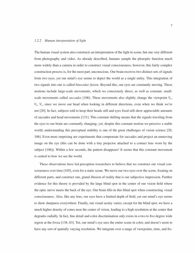
Figure 1.1: Demonstrations of perceptual constancy. The first image, created by Edward Adelson, demon-strates brightness constancy. The two checkers labeled A and B are of the same brightness; however, weperceive B as lighter than A because our brains automatically discount illumination effects. The next twoimages demonstrate size constancy. In the middle image, the black cylinder is the same size as the third whitecylinder. In the final image, all three cylinders are the same size. The depth cues in the images cause ourbrains to account for perspective foreshortening, and thus we perceive these sizes differently.

ation locations, forming a stable perception of the scene from the very unstable stimuli originating

in the eyes.

Visual consciousness also seems to have some amount of interpretation built-in; when perceiving

a scene we have impressive capabilities for discounting confounding effects such as illumination

and perspective foreshortening. In perception science, this capability is called constancy [106]. A

powerful example of brightness constancy is shown in Figure 1.1. We perceive the white checker in

the shadow(marked B) as lighter than the dark checker (marked A) outside the shadow, when in fact

these areas have the same luminance. Our mind’s eye manages to discount illumination effects so

that we can perceive the true reflectances of the scene. Size constancy refers to our ability to perceive

the true size of objects regardless of their distance from us. A classic example [48] is when we look

at our face in a mirror; the size of the image on the surface of the mirror is half the size of our

real face. When informed of this, most people will disagree vigorously until they test the hypothesis

in front of a mirror. Most people are likewise surprised by the demonstration of size constancy in

Figure 1.1. Shape constancy refers to our ability to perceive the true shape of objects even though

their shape on the retina might be very different due to perspective effects. Note that constancy is

not a defect of our visual system; constancy helps us to interpret the light that enters our retinas and

9

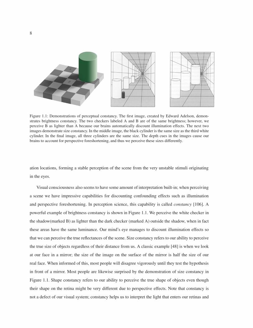
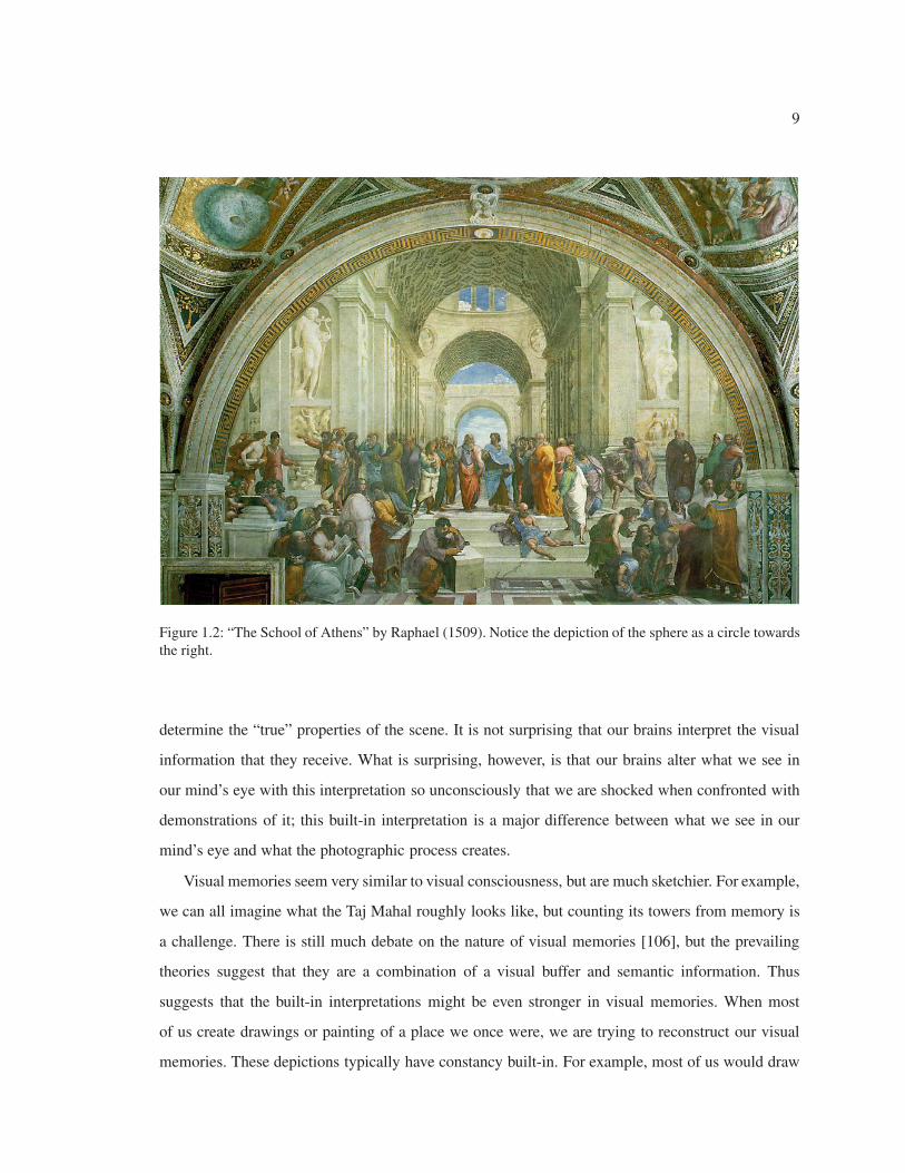
Figure 1.2: “The School of Athens” by Raphael (1509). Notice the depiction of the sphere as a circle towardsthe right.

determine the “true” properties of the scene. It is not surprising that our brains interpret the visual

information that they receive. What is surprising, however, is that our brains alter what we see in

our mind’s eye with this interpretation so unconsciously that we are shocked when confronted with

demonstrations of it; this built-in interpretation is a major difference between what we see in our

mind’s eye and what the photographic process creates.

Visual memories seem very similar to visual consciousness, but are much sketchier. For example,

we can all imagine what the Taj Mahal roughly looks like, but counting its towers from memory is

a challenge. There is still much debate on the nature of visual memories [106], but the prevailing

theories suggest that they are a combination of a visual buffer and semantic information. Thus

suggests that the built-in interpretations might be even stronger in visual memories. When most

of us create drawings or painting of a place we once were, we are trying to reconstruct our visual

memories. These depictions typically have constancy built-in. For example, most of us would draw

10

a sphere as a circle, even though the rules of perspective require an ellipse (assuming the sphere is

not perfectly at the center of the image). A famous example of depicting a sphere as a circle can be

seen in Raphael’s painting “The School of Athens” (Figure 1.2). If this sphere had been depicted as

an ellipse, we probably would have thought it was egg-shaped in 3D. Likewise, most of us would

paint the scene in Figure 1.1 with square B lighter than square A.

The depiction we see in our mind’s eye seems very powerful. It has a high dynamic range and

wide field of view. It is sharp and has good depth of of field. Our mind’s eye seems to have some

built-in interpretation that reflects the 3D nature of our world and discounts confounding factors

such as illuminant color and perspective foreshortening. We know that this depiction is constructed

from multiple samples of the plenoptic function captured by our two eyes, over a range of time and

saccadic movements. Thus, it is not surprising that there is a large divide between the outputs of

our cameras and the plenoptic function that we experience during visual consciousness; cameras

and humans interpret the plenoptic function in different ways. The large variety of possibilities in

interpreting the plenoptic function motivates an obvious question: can we use digital technology to

bridge this divide, and move beyond the limitations of traditional cameras to produce more effective

depictions? In the next chapter I describe one approach to addressing this challenge, which begins

by capturing a much wider sampling of the plenoptic function than a camera would. This approach

then combines this wider sampling into depictions that are more effective than traditional images or

videos.

11

Chapter 2

A FRAMEWORK

Computer graphics as a field has traditionally concerned itself with depicting reality by mod-

eling and rendering it in three dimensions in a style as “photo-realistic” as possible. Computer

vision as a field has traditionally concerned itself with understanding and measuring reality through

the analysis of photographic images. In the past, computer scientists have paid little attention to

the problems of depicting and communicating reality through photography, precisely because pho-

tographs already provide such a powerful illusion of reality with little user expertise or effort. Just

because a photograph is inherently “photo-realistic”, however, does not mean that it is effective at

depicting what the author hoped to depict. We have seen in the previous chapter that photographs

are interpretations of reality. Unfortunately, however, they may not be the interpretation we want;

thus, even though photographs are already photo-realistic there is considerable latitude to increase

their effectiveness. This observation, coupled with photography’s ease of use and the recent explo-

sion of cheap, consumer-level digital cameras, has made photographic depiction of reality a new

and exciting area of research.

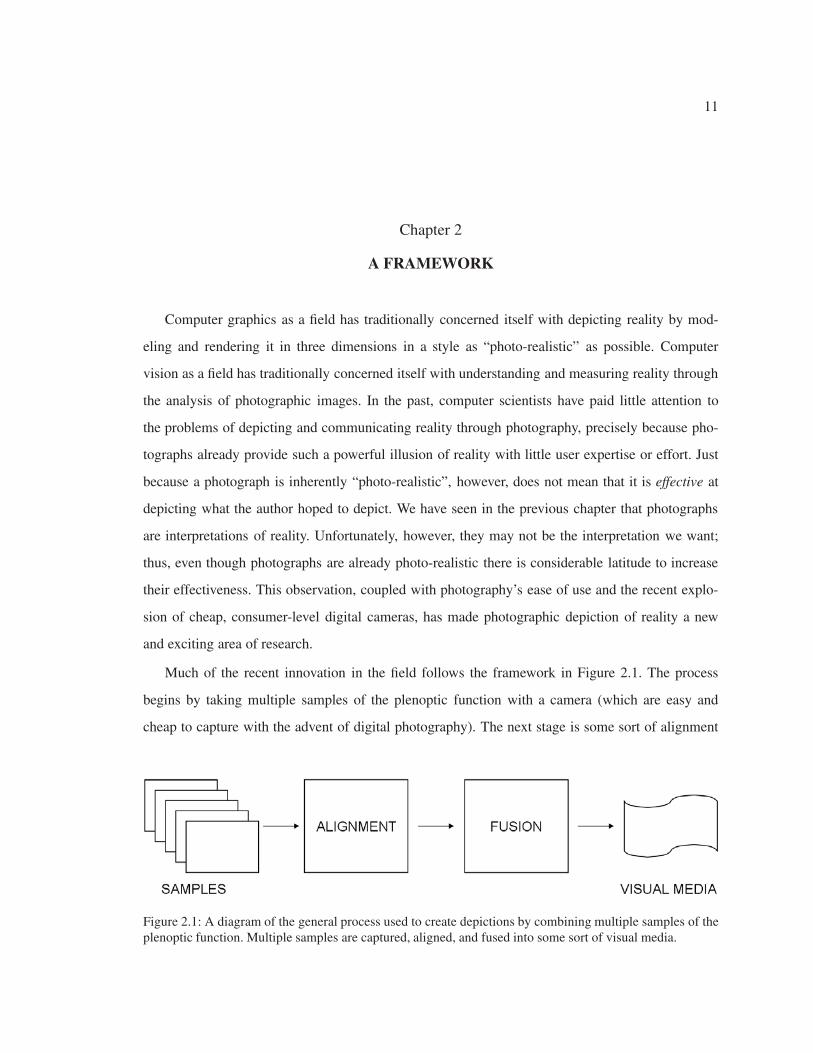
Much of the recent innovation in the field follows the framework in Figure 2.1. The process

begins by taking multiple samples of the plenoptic function with a camera (which are easy and

cheap to capture with the advent of digital photography). The next stage is some sort of alignment

Figure 2.1: A diagram of the general process used to create depictions by combining multiple samples of theplenoptic function. Multiple samples are captured, aligned, and fused into some sort of visual media.

12

or registration process that is applied to the samples in order to position them into a single frame of

reference. Next, the aligned samples are integrated or fused into one entity. The final output of the

process is some sort of visual media. This media could resemble a photograph or video, or take the

form of something more complex that requires a specialized viewer.

Note that this process description is coarse, and some techniques will not strictly follow it. The

notion of multiple samples is meant to be broad. For example, a single video sequence can be

considered as multiple photographs, or even multiple videos if it is split into sub-sequences. Also,

I will sometimes misuse the notion of a single sample to mean a simple sample; i.e., a traditional

photograph or video. This is useful to describe specialized hardware devices that instantaneously

capture a single but complex sample of the plenoptic function that contains as much information as

several traditional photographs or videos.

2.1 My approach

A large body of work fits within the framework in Figure 2.1, and there are many alternatives for

the alignment and fusion steps (as I will survey in Section 2.2). My thesis projects, however, all

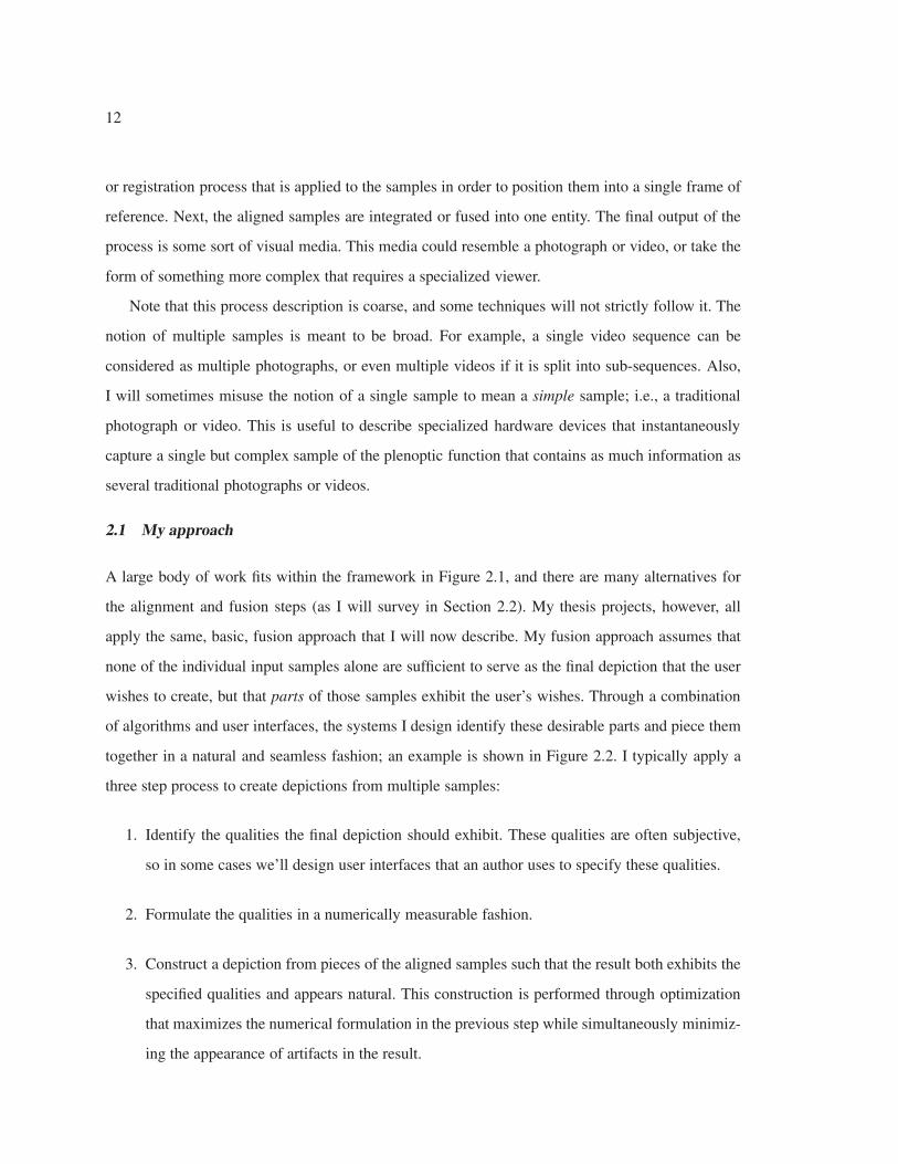
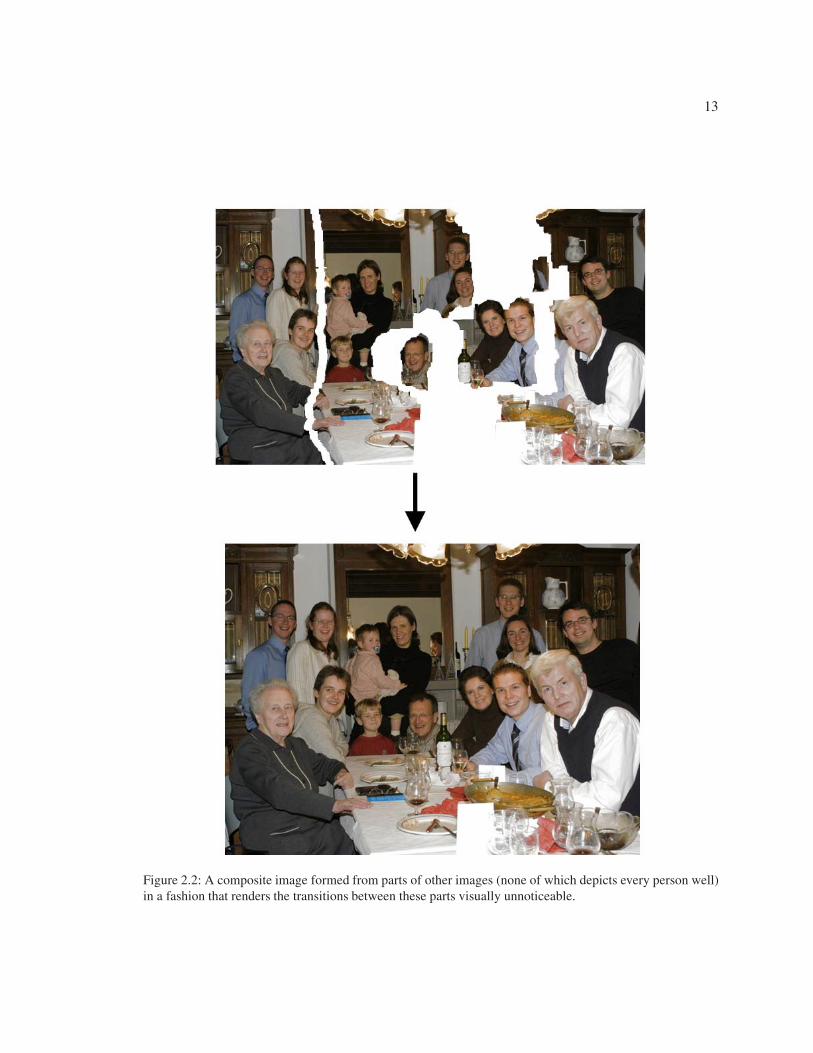
apply the same, basic, fusion approach that I will now describe. My fusion approach assumes that

none of the individual input samples alone are sufficient to serve as the final depiction that the user

wishes to create, but that parts of those samples exhibit the user’s wishes. Through a combination

of algorithms and user interfaces, the systems I design identify these desirable parts and piece them

together in a natural and seamless fashion; an example is shown in Figure 2.2. I typically apply a

three step process to create depictions from multiple samples:

1. Identify the qualities the final depiction should exhibit. These qualities are often subjective,

so in some cases we’ll design user interfaces that an author uses to specify these qualities.

2. Formulate the qualities in a numerically measurable fashion.

3. Construct a depiction from pieces of the aligned samples such that the result both exhibits the

specified qualities and appears natural. This construction is performed through optimization

that maximizes the numerical formulation in the previous step while simultaneously minimiz-

ing the appearance of artifacts in the result.

13

Figure 2.2: A composite image formed from parts of other images (none of which depicts every person well)in a fashion that renders the transitions between these parts visually unnoticeable.

14

I apply this three step process in three different projects discussed in chapters 3- 5. In chapter 3

I describe an interactive, computer-assisted framework for combining parts of a set of photographs

into a single composite picture, a process I call “digital photomontage.” Central to the framework

is a suite of interactive tools that allow the user to specify high-level goals for the composite, either

globally across the image, or locally through a painting interface. The power of this framework lies

in its generality; I show how it can be used for a wide variety of applications, including “selective

composites” (for instance, group photos in which everyone looks their best), relighting, extended

depth of field, panoramic stitching, clean-plate production, stroboscopic visualization of movement,

and time-lapse mosaics. Also, in this chapter I introduce the two technical components that allow me

to accomplish steps 2 and 3 for each of the three projects. In step 2, I formulate the qualities the de-

piction should exhibit as a cost function that takes the form of a Markov Random Field (MRF) [45].

In step 3 I minimize this cost function using graph cuts [18]. The result of this minimization speci-

fies which part of a source sample to use for each pixel of the output depiction. Rather than simply

copy colors from the sources to create a depiction, in many cases improved results can be achieved

by compositing in the gradient-domain [108].

For the most part, I assume in chapter 3 that each source photograph is captured from the same

viewpoint. In chapter 4 I extend the photomontage framework to multiple viewpoints, in the context

of creating multi-viewpoint panoramas of very long, roughly planar scenes such as the facades

of buildings along a city street. This extension requires a different image registration step than in

chapter 3, as well as a technique for projecting the source images into a new reference frame such

that some image regions are aligned. I then formulate the qualities these panoramas should exhibit

in a similar mathematical form as the cost functions in the photomontage system, but customized

to the case of panoramas of long scenes (the same graph cut optimization and gradient-domain

compositing steps are then employed). I also describe a different suite of interactive tools that an

author can use to improve the appearance of the result.

Finally, in chapter 5 I apply this three step process to video inputs. Specifically, I describes a

mostly automatic method for taking the output of a single panning video camera and creating a

panoramic video texture (PVT): a video that has been stitched into a single, wide field of view and

that appears to play continuously and indefinitely. In this case, the qualities the depiction should

exhibit are straight-forward and not subjective. Instead, the key challenge in creating a PVT is that

15

although only a portion of the scene has been imaged at any given time, the output must simultane-

ously portray motion throughout the scene. Like the previous two chapters, I use graph cut optimiza-

tion to construct a result from fragments of the inputs. Unlike the previous chapters, however, these

fragments are three-dimensional because they represent video, and thus must be stitched together

both spatially and temporally. Because of this extra dimension, the optimization must take place over

a much larger set of data. Thus, to create PVTs, I introduce a dynamic programming step, followed

by a novel hierarchical graph cut optimization algorithm. I also use gradient-domain compositing in

three dimensions to further smooth boundaries between video fragments. I demonstrate my results

with an interactive viewer in which users can interactively pan and zoom on high-resolution PVTs.

2.2 Previous work

Before describing my approach in detail over the next three chapters, I first discuss related work

within the context of the general framework in Figure 2.1. The common goal of the work I describe

is to create more effective depictions starting with simple samples of visual reality; however, the

work varies in techniques, inputs, and outputs. Perhaps more importantly, there are varying ways a

depiction can be made more effective. Most of the work I will describe tries to help people (espe-

cially amateurs) capture and create imagery that better matches their visual memories. Other work,

however, has the goal of creating imagery that visualizes and communicates specific information

about a scene, such as motion or shape.

2.2.1 Depiction that better matches what we perceive

As discussed in Chapter 1, photographs and video convey an illusion of reality, but are often very

different than what we perceive. This can be frustrating when we take snapshots and movie clips with

the goal that they will match our visual memories; thus, the goal of this research area is to create

visual media better aligned to human visual perception. Our visual perception system integrates

information from multiple visual samples; thus the natural technical approach is to capture multiple

samples of the plenoptic function and somehow integrate them into an output that better depicts the

scene.

One of the most difficult limitations of photography and video is its limited dynamic range. As

16

already discussed, a photographic emulsion or digital sensor is able to record a much smaller range

of radiances than the human eye. Radiances below this range yield black, and radiances above this

range yield white; radiances in-between are mapped non-linearly to the final brightnesses in the

image. Thus, photographs typically have much less detail in shadow and highlight regions than the

human eye would normally perceive. A natural approach is to take multiple images under varying

exposure settings, and combine them into one higher dynamic range image (often called a radiance

map). Care must be taken not to move the camera between exposures; otherwise, a spatial alignment

step must first be performed. The next step in the process is radiometric calibration, which solves

for a mapping between each source image’s brightness and the scene radiance values (this can

be considered an alignment step in radiometric space). Finally, the images are combined into one

high-dynamic range radiance map. The most common approaches to creating radiance maps were

proposed by Mann and Picard [86], Debevec and Malik [33], and Mitsunaga and Nayar [91].

Unfortunately, computer display devices and paper prints cannot portray high-dynamic range

(though high-dynamic range LCD displays are starting to appear [126]); thus, a related problem is

the compression of radiance maps into regular images that still portray all the perceptually relevant

details of the scene [138, 34, 38, 117]. This compression step completes the overall process; the

input consists of multiple images with limited dynamic range, and the output is an image that better

depicts the dynamic range that humans visually perceive.

Combining multiple exposures of a scene requires that the scene and camera remain static; sev-

eral researchers have explored the problem of creating high-dynamic range videos and photographs

of moving scenes. Kang et al. [68] use a video camera with rapidly varying exposures and optical

flow to align adjacent frames before integrating their information. Nayar and students demonstrate

several novel hardware systems that are able to instantaneously collect high-dynamic range infor-

mation. These devices include sensors with spatially varying pixel exposures [98], cameras with a

spatially-varying sensor such that camera rotation yields panoramas with multiple samples of radi-

ance for each pixel [123], and cameras with a dynamic light attenuator that changes spatiotemporally

to yield high-dynamic range video [97].

Capturing effective imagery in low light conditions is challenging because the signal-to-noise

ratio improves when more light enters the camera; thus, low-light imagery tends to be noisy. In

contrast, humans can perceive scenes in very low light conditions. The images in our mind’s eye

17

do not seem to contain anything resembling film or digital graininess (though human low-light per-

ception is mostly achromatic [83]). One approach to capturing photographs in low light is to use

a long exposure time, which increases the total light impinging on the sensor. Unfortunately, mo-

tion blur results if the camera is moving, or if there is motion in the scene. Ezra and Nayar [13]

address the problem of motion blur by simultaneously capturing two samples of the plenoptic func-

tion; one high-resolution photograph, and one low-resolution video. Alignment is performed on the

video frames to recover camera motion; this motion is then used to deconvolve the high-resolution

photograph and remove the motion blur. Jia et al. [65] instead capture two photographs; one under-

exposed image captured with a short shutter time, and one long exposure image that contains motion

blur. The colors of the long exposure are then transferred to the under-exposed image. They assume

only minor image motion in-between the two photographs; however, their technique does not re-

quire pixel-to-pixel alignment. Motion blur can be removed from a single image using a variational

learning procedure that takes advantage of the statistics of natural images [39]. Active illumination

is the most common approach to low-light photography; a camera-mounted flash is used to illumi-

nate the scene for a brief moment while the sensor is exposed. This approach reduces noise, but

unfortunately results in images that are very different than we perceive. Flash changes the colors of

the scene, adds harsh shadows, and causes a brightness fall-off with increasing distance from the

flash. Thus, Petschnigg et al. [109] and Eisemann and Durand [35] show that fusing two images of

the scene, one with flash and the other without, can result in a more effective and clear photograph.

The authors capture the no-flash image with a short enough exposure to avoid motion blur, and then

fuse it with the low noise of the flash image. If the camera is not on a tripod, spatial alignment is

first required. Other artifacts of flash, such as reflections, highlights, and poor illumination of dis-

tant objects can also be corrected using a flash/no-flash pair [6]. Finally, Bennett and McMillan [15]

address the problem of taking videos of scenes with very little light. They first align the frames of

a moving camera, and then integrate information across the multiple registered frames to reduce

noise.

Another problem with photography and especially video is resolution; visual imagery often

does not contain enough information to resolve fine details. As already discussed, our eyes have

their finest resolving power and color perception only in the fovea. We constantly move our eyes

over a scene, and our brains construct a single high-resolution perception from this input without

18

conscious effort. Thus, a natural approach to increasing the sampling of the plenoptic function that

a photograph or video represents is to combine multiple samples. Approaches to this problem [64,

36, 125, 87] begin with either multiple, shifted photographs, or a video sequence with a moving

camera (recent advances in still photography resolution make the case of video significantly more

relevant than still image input). Spatial alignment is performed to align the multiple samples with

subpixel accuracy. Finally, information from the different aliasing of the subpixel-shifted, multiple

samples can be integrated into a high-resolution image. An alternate, hardware-based approach is

to mechanically jitter the digital sensor while recording video [14] in order to acquire multiple,

shifted samples while avoiding the motion blur induced by a moving video camera (the shifts are

done between frame exposures). These multiple samples can then be integrated to create higher

resolution. Finally, Sawhney et al. [122] show how to transfer resolution between a stereo pair of

cameras, where one camera captures high resolution and the other low.

Along with limited resolution, video suffers from its finite duration. While a photograph of

a scene can seem timeless, a video represents a very specific interval of time; this is natural for

storytelling, but isn’t effective for creating a timeless depiction of a scene. For example, imagine

communicating the appearance of a nature scene containing waving trees, a waterfall, and rippling

water. A photograph will not communicate the dynamics of the scene, while a video clip will have

a beginning, middle, and end that aren’t relevant to the goal of the depiction. Schodl et al. [124]

demonstrate a new medium, the video texture, that resides somewhere between a photograph and

a video. Video textures are dynamic, but play forever; they are used to depict repetitive scenes

where the notion of time is relative. Their system identifies similar frames in the input video that

can serve as natural transitions. The input video is then split into chunks between these transition

frames (thus forming multiple samples of the plenoptic function), and these chunks are played in a

quasi-random order for as long as the viewer desires. Video textures can be seen as hallucinating an

infinite sampling of the time dimension of the plenoptic function. In later work, Kwatra et al. [77]

shows that more complex spatiotemporal transitions between input chunks can produce seamless

results for more types of scenes. In general, the alignment stage is skipped for video textures since it

is assumed that the camera is stationary; this assumption is relaxed in chapter 5, where I show how

to extend video textures to a panoramic field of view from the input of a single video camera.

As discussed in the introduction, the sharp, rectangular frame of a photographic image or video

19

is quite different than what humans visually perceive. A single human eye see its fullest resolution

and color discrimination at the fovea, and these capabilities degrade quickly towards the periphery.

However, given two eyes and saccadic motion, our perception is that of a very large field of view.

Panoramic photography, which creates photographs with a wider field of view, has existed since

the late 19th century [89]; more recently, digital techniques for creating panoramas have become

popular. In this approach, multiple photographs are captured from a camera rotating about its nodal

point, and composited into a single image. Thus, multiple samples of the plenoptic function are

combined to a create single result with an increased sampling compared to a traditional photograph.

The first stage of this process is, as usual, alignment. The direction of view of each photograph is

recovered so that the images are in one space. Then, the images are projected onto a surface (usu-

ally a plane, cylinder, or sphere); finally, the images are composited (this step is necessary because

the source images overlap). In the case of cylindrical or spherical panoramas, the resultant media

may be viewed with an interactive viewer that allows the user to rotate and look around within the

scene [27]. There is a significant volume of research on digital panoramic techniques, so I men-

tion only a few, notable examples. One of the first successful and complete approaches to creating

full-view panoramas was developed by Szeliski and Shum [134]. More recently, feature-based tech-

niques for alignment [22] have completely automated the alignment step. A variety of compositing

techniques exist for combining the aligned images. Compositing problems can arise from motion in

the scene while the images are captured, and from exposure variations between the images. Blending

across exposure differences was traditionally handled with Laplacian pyramids [103]; more recently,

gradient-domain techniques have become popular [78]. Motion can be handled with optimal seam

placement through dynamic programming [32], or vertex-cover algorithms [141]. In chapter 3 I

show how motion and exposure differences can be simultaneously handled using graph cuts and

gradient-domain fusion.

Human visual perception sees a dynamic scene in a wide field of view. Thus, a natural exten-

sion to panoramic images is panoramic video. This extension increases the sampling of the plenop-

tic function contained in the visual media to a level that better approximates human vision. One

approach to creating panoramic video is to place multiple, synchronized video cameras into a sin-

gle hardware unit; several companies sell such specialized devices (e.g., [110]), but they are typ-

ically very expensive. Several researchers have explored the depiction possibilities of panoramic

20

video [140, 99, 71]. Another approach is to attach a special mirror and lens device to a standard

video camera [96] to capture a coded version of the full, spherical field of view. This coded input is

then unwarped into a panoramic video. The limitation of this approach is that the resultant video is

less than the resolution of the video camera, due to non-uniform sampling; this limitation is signifi-

cant given the already low resolution of video cameras. I will describe my own approach to creating

high-resolution panoramic video textures from the input of a single video camera in chapter 5.

Creating still photographs that depict moving scenes is a challenge because a photograph is

inherently static. Photography has long had an unique relationship with time. The first cameras re-

quired very long exposure times, which essentially wiped out any moving elements. Photographs of

city blocks removed moving people, much to the surprise and sometimes chagrin of early photogra-

phers [100]. Over time, newer technology allowed the introduction of shorter and shorter exposure

times; the result was the ability to “freeze” time. Frozen images of rapidly moving scenes can be

highly informative; we discuss the educational ramifications of motion photography in Section 2.2.2.

However, such frozen images often do a poor job of evoking motion; they appear oddly static. It can

be argued that this inadequacy arises because such images don’t look anything like what we per-

ceive when viewing a moving scene. Because the human eye has sharp spatial precision and color

discrimination only within the three to five degree region at the center of the eye, a depiction of the

entire field of view of a moving scene in sharp detail is incompatible with what we perceive. Instead,

artists use a number of techniques that take advantage of human visual perception to suggest motion

in a static form; Cutting [30] provides an excellent survey of these techniques. Livingstone [83]

contends that impressionist paintings of moving scenes better resemble human perception of mo-

tion because they exhibit similar spatial imprecision; she also argues that the use of equiluminant

colors conveys an illusion of motion when used to depict subtly moving areas such as rippling wa-

ter. Motion blur is quite similar to what we perceive when viewing quickly moving scenes. Motion

blur results in photographs of spinning wheels that are blurrier than their surroundings, and streaks

when objects move across the scene rapidly. These effects are highly evocative of motion. Depicting

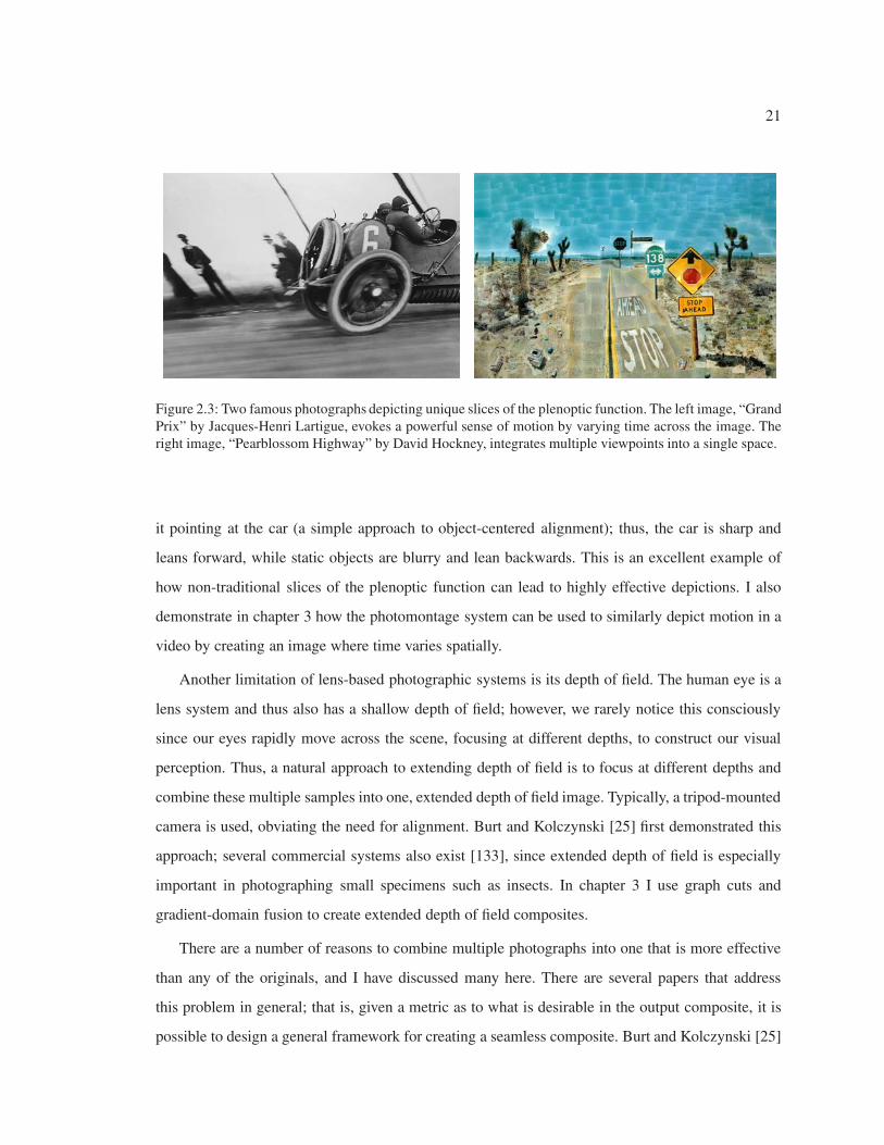
moving objects as leaning into their direction of travel also seems to suggest motion. Jacques-Henri

Lartigue’s famous photograph in Figure 2.3 strongly evokes motion, and is actually a very unique

slice of the plenoptic function. He used a special camera with a rolling shutter, such that time travels

continuously forward from the bottom to the top of the image. He also panned the camera to keep

21

Figure 2.3: Two famous photographs depicting unique slices of the plenoptic function. The left image, “GrandPrix” by Jacques-Henri Lartigue, evokes a powerful sense of motion by varying time across the image. Theright image, “Pearblossom Highway” by David Hockney, integrates multiple viewpoints into a single space.

it pointing at the car (a simple approach to object-centered alignment); thus, the car is sharp and

leans forward, while static objects are blurry and lean backwards. This is an excellent example of

how non-traditional slices of the plenoptic function can lead to highly effective depictions. I also

demonstrate in chapter 3 how the photomontage system can be used to similarly depict motion in a

video by creating an image where time varies spatially.

Another limitation of lens-based photographic systems is its depth of field. The human eye is a

lens system and thus also has a shallow depth of field; however, we rarely notice this consciously

since our eyes rapidly move across the scene, focusing at different depths, to construct our visual

perception. Thus, a natural approach to extending depth of field is to focus at different depths and

combine these multiple samples into one, extended depth of field image. Typically, a tripod-mounted

camera is used, obviating the need for alignment. Burt and Kolczynski [25] first demonstrated this

approach; several commercial systems also exist [133], since extended depth of field is especially

important in photographing small specimens such as insects. In chapter 3 I use graph cuts and

gradient-domain fusion to create extended depth of field composites.

There are a number of reasons to combine multiple photographs into one that is more effective

than any of the originals, and I have discussed many here. There are several papers that address

this problem in general; that is, given a metric as to what is desirable in the output composite, it is

possible to design a general framework for creating a seamless composite. Burt and Kolczynski [25]

22

were the first to suggest such a framework; they use a salience metric along with Laplacian pyramids

to automatically fuse source images. They demonstrate some of the first results for extended depth

of field, high dynamic range, and multi-spectral fusion. In chapter 3, I show how salience metrics

and user interaction coupled with graph cuts and gradient-domain fusion can yield better results for

a wide variety of problems.

Many of the projects in the preceding paragraphs begin with multiple photographs with varying

parameters and align them spatially; given this input, a wide range of effects and depictions can

be created [3]. This approach is difficult to apply to video, given the difficulty of aligning two

video sequences; the frames of the two video sequences would have to be aligned both spatially and

temporally. Sand and Teller [121] thus present their video matching system to address the problem

of spatiotemporal video alignment. Their work focuses on the alignment phase of my framework,

but also demonstrates that a wide range of effects can be created using simple techniques once

the alignment is computed. These effects included high-dynamic range, wide field of view, and a

number of visual effects that are useful for films.

Photographs obey the laws of perspective and depict a scene from a single viewpoint; our mind’s

eye, however, integrates multiple viewpoints. Our visual consciousness may resemble a photograph,

but it actually integrates two viewpoints from our two eyes. Also, as we move our eyes over a scene

to build our perception of it, our heads move [131]. If we are walking, this integration of multiple

viewpoints is accentuated. Also, our mind’s eye has some interpretation built-in, and discounts some

perspective effects. Thus, given the departures of our mind’s eye from strict perspective, the best de-

piction of a scene may not be a perspective photograph. Artists have a long history of incorporating

multiple perspectives in paintings to create better depictions [76, 59]. Artist David Hockney creates

photocollages such as “Pearblossom Highway” (Figure 2.3) that show multiple viewpoints in the

same space because he feels that they better match human visual perception [58]. Krikke [75] ar-

gues that axonometric perspective, which is an oblique orthographic projection used in Byzantine

and chinese paintings, as well as many modern video games such as SimCity, presents imagery that

resembles human visual consciousness. Axonometric perspective is more similar to what we “know”

rather than what we “see”; parallel lines are parallel, and objects are the same size regardless of their

distance from the viewer (which resembles the effects of size constancy in human visual perception).

We can comprehend axonometric images even though they appear very different from the input to

23

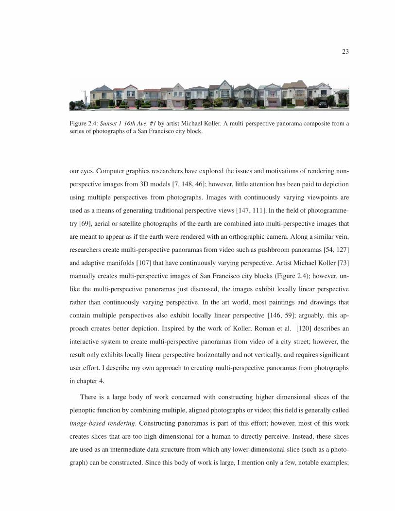
Figure 2.4: Sunset 1-16th Ave, #1 by artist Michael Koller. A multi-perspective panorama composite from aseries of photographs of a San Francisco city block.

our eyes. Computer graphics researchers have explored the issues and motivations of rendering non-

perspective images from 3D models [7, 148, 46]; however, little attention has been paid to depiction

using multiple perspectives from photographs. Images with continuously varying viewpoints are

used as a means of generating traditional perspective views [147, 111]. In the field of photogramme-

try [69], aerial or satellite photographs of the earth are combined into multi-perspective images that

are meant to appear as if the earth were rendered with an orthographic camera. Along a similar vein,

researchers create multi-perspective panoramas from video such as pushbroom panoramas [54, 127]

and adaptive manifolds [107] that have continuously varying perspective. Artist Michael Koller [73]

manually creates multi-perspective images of San Francisco city blocks (Figure 2.4); however, un-

like the multi-perspective panoramas just discussed, the images exhibit locally linear perspective

rather than continuously varying perspective. In the art world, most paintings and drawings that

contain multiple perspectives also exhibit locally linear perspective [146, 59]; arguably, this ap-

proach creates better depiction. Inspired by the work of Koller, Roman et al. [120] describes an

interactive system to create multi-perspective panoramas from video of a city street; however, the

result only exhibits locally linear perspective horizontally and not vertically, and requires significant

user effort. I describe my own approach to creating multi-perspective panoramas from photographs

in chapter 4.

There is a large body of work concerned with constructing higher dimensional slices of the

plenoptic function by combining multiple, aligned photographs or video; this field is generally called

image-based rendering. Constructing panoramas is part of this effort; however, most of this work

creates slices that are too high-dimensional for a human to directly perceive. Instead, these slices

are used as an intermediate data structure from which any lower-dimensional slice (such as a photo-

graph) can be constructed. Since this body of work is large, I mention only a few, notable examples;

24

see Kang and Shum [66] for a survey. Light field rendering [81] and the Lumigraph [52, 24] con-

struct a complete 4D sample of the plenoptic function and thus are able to render photographs of

a static scene from any viewpoint outside the scene’s convex hull. Capturing videos from multiple

viewpoints and constructing interpolated views allows users to see a dynamic scene from the view-

point of their choice [151, 112]. Large arrays of cameras can be used to acquire multiple samples

and simulate denser samplings along one or more axes of the plenoptic function, such as spatial res-

olution, dynamic range, and time (video frame rate) [80, 145]. These systems, along with a recent

hand-held light field camera [101], can also simultaneously sample at different focusing planes and

simulate a wide range of depths of field.

2.2.2 Communicating information

A common reason to depict reality is to communicate specific information; examples include surveil-

lance imagery, medical images, images that accompany technical instructions, educational images

such as those found in textbooks, forensic images, and photographs of archaeological specimens.

Sometimes a simple photograph is very effective for the desired task. In other cases, such as tech-

nical illustration [49], non-realistic depiction can prove to be more effective. The field of non-

photorealistic rendering (NPR) [50] contains a wealth of techniques to create non-photorealistic

imagery that can communicate more effectively than realistic renderings.

Given that a simple photograph or video may not be the most effective at communicating the

goal of the author, there are several projects that combine multiple samples of the plenoptic func-

tion to convey information. Typically, these approaches assume that the samples are taken from a

camera on a tripod, thus skipping the alignment phase. Burt and Kolczynski [25] demonstrate that

combining infrared imagery with visible spectrum photographs is helpful for surveillance tasks or

for landing aircraft in poor weather. Raskar et al. [113] take two videos or images of a scene under

different illumination; typically under daylight and moonlight. Then, the low-light nighttime video

is enhanced with the information of the daylight imagery, in order to make it more comprehensible.

They demonstrate the usefulness of this approach for surveillance. Akers et al. [8] note that lighting

of complex objects such as archaeological specimens in order to convey shape and surface texture is

a challenging task; as a result, many practitioners prefer technical illustrations. In their system, they

25

begin with hundreds of photographs from the same viewpoint but with a single, varying light source

(the position of the light source is controlled by a robotic arm); these images are then composited

interactively by a designer to create the best possible image. Their system requires significant user

effort in choosing lighting directions. My own approach to this problem using the photomontage

framework is described in chapter 3. In more recent work, Mohan et al. [92] describe a table-top rig

and software for controlling the lighting of complex objects. The rig first captures low-resolution

images for a wide range of lighting directions; the user then sketches the desired lighting. This

sketch is approximated as a weighted sum of several source images, which are finally re-captured at

high-resolution to create a final result.

Along with relighting, multiple images under varying illumination can be useful for a variety

of tasks. An intrinsic image [12] decomposes a photograph into two images; one showing the re-

flectance of the scene, and the other showing the illumination. Recovering intrinsic images from a

single photograph is ill-posed; however, given multiple images of the scene under varying illumina-

tion, the decomposition becomes easier [143]. Intrinsic images are most often used to communicate

the reflectance of the scene without the confounding effects of illumination (much like human per-

ception compensates for the effects of illumination); but they can also be used for depiction. For

example, one can modify a scene’s reflectance and then re-apply the illumination to achieve more

realistic visual effects. Finally, we have already seen that combining a flash and no-flash image can

create a more effective depiction. Raskar et al. [114] show that a no-flash image plus four flash

images in which the flash is located to the left, right, top, and bottom of the camera lens can yield

highly accurate information about the depth discontinuities of the scene. Rather than directly inte-

grate these five images, they use them to infer information. This information is then applied to one

of the images to increase its comprehensibility. For example, photographs can be made to look more

like technical illustrations or line drawings, improving their depiction of shape.

Conveying the details of moving scenes is also an interesting depiction challenge. I discussed in

Section 2.2.1 how photographs of motion depict frozen moments in time and appear quite different

than what we perceive; I then surveyed techniques to create images that suggest motion. In contrast,

such frozen moments in time can be very educational precisely because we cannot perceive them;

they reveal and communicate details about rapid movements that the human eye cannot discern.

Eadward Muybridge captured some of the first instantaneous photographs [95]; he photographed

26

quickly moving subjects at a rapid rate, and laid out the images like frames of a comic book. These

visualizations of motion communicated the mechanics of motion, and the result was surprising;

the popular conception of a galloping horse, as seen in many paintings, turned out to be incorrect.

Harold Edgerton [70] developed the electronic flash, and shocked the world with images of a drop

of milk splashing, and a bullet bursting through an apple. Dayton Taylor [135] photographs rapidly

moving scenes with rails of closely-spaced cameras; this results in the ability to capture a frozen a

moment from multiple angles1. The output is a unique slice of the plenoptic function; a movie that

depicts a single moment of time from multiple viewpoints. The ability to rotate a frozen moment

is, of course, nothing that a human could perceive if he/she were standing there; thus, the effect

can be both shocking and highly informative. This technology has been used in several films and

television advertisements, such as the famous bullet-time sequence in the Matrix. A dense array of

cameras can also be used to capture extremely high frame rate video [145]. This frame rate allows

rapidly evolving phenomena such as a bursting balloon to be visualized not just at an instant, as in

Edgerton’s work, but over a short range of time.

Stroboscopic images combine multiple samples of a scene over a short range of time into a

single image that communicates motion. Some of the first stroboscopic photographs were created

by Jules-Etienne Marey [19]. Salient Stills [87] are single images that depict multiple frames of a

video sequence; they are created by aligning and then compositing the video frames. Their resultant

images are often stroboscopic. My photomontage system (chapter 3) provides another approach to

creating seamless stroboscopic images from video. Assa et al. [9] present a system for automatically

selecting the key poses of a character in a video or motion capture sequence to create a stroboscopic

image that visualizes its motion. Cutting [30] points out that stroboscopy in art can be found as early

as the paleolithic era, and that even preschoolers can understand stroboscopic visualization. This

universal comprehensibility of stroboscopy is perhaps surprising, since human visual perception

does not seem to resemble it.

Stroboscopy is not the only way to convey information about motion. Motion lines, such as

those found in comic books [88], are a diagrammatic approach to communicating motion. Motion

lines seem to be a universally comprehensible metaphor for motion, but they are not believed to bear

1More widely spaced cameras are possible using algorithms that reconstruct the depth of the scene in order to inter-polate novel viewpoints [151].

27

much resemblance to visual perception of motion. Shape-time photography [43], like stroboscopy,

takes a video sequence of a moving object and composites the movement into a single image. How-

ever, rather than depicting a uniform sampling over time, their composite shows the object surface

that was closest to the camera over all time frames. Film storyboards are drawn using an established,

visual language for conveying details about motion. Goldman et al. [47] use this language to au-

tomatically summarize the content of a short video clip in static form. Finally, some motions in a

video sequence are too small for the human eye to perceive; motion magnification [82] amplifies

these motions to better visualize them.

2.2.3 What doesn’t fit?

It may seem from the previous sections that nearly every technique fits the framework in Figure 2.1.

Indeed, it is a more commonly followed process than I originally thought. However, there are tech-

niques that lie outside of the framework. Many techniques operate on a single photograph or video,

and attempt to hallucinate the information that would be provided by multiple samples in order to

enrich the depiction. Tour into the Picture [61], for example, creates the illusion of 3D navigation

from a single photograph or painting. Oh et al. [104] take a similar approach to the interactive

authoring of 3D models from a single photograph. Both of these systems require significant user

effort; Hoiem et al. [60] present a completely automatic approach to the same problem. Chuang et

al. [29] apply hallucinated motion to single photographs or video to make them seem like video

textures. Zorin and Barr [153] notice that wide-angle lens create photo-realistic but perceptually

distorted images; they apply a warp to such images to improve the depiction.

These approaches are able to create compelling results, especially on older paintings and pho-

tographs for which we have no additional samples of the plenoptic function. However, the ubiquity

of digital sensors and their economy of scale suggest that acquiring multiple samples of the plenoptic

function is a better approach for depicting existing scenes.

In the next three chapters I describe my own research into creating better depictions by integrat-

ing multiple samples of the plenoptic function.

28

Chapter 3

INTERACTIVE DIGITAL PHOTOMONTAGE

The means by which these pictures could have been accomplished is Combination

Printing, a method which enables the photographer to represent objects in different

planes in proper focus, to keep the true atmospheric and linear relation of varying dis-

tances, and by which a picture can be divided into separate portions for execution, the

parts to be afterwards printed together on one paper, thus enabling the operator to de-

vote all his attention to a single figure or sub-group at a time, so that if any part be

imperfect from any cause, it can be substituted by another without the loss of the whole

picture, as would be the case if taken at one operation. By thus devoting the attention to

individual parts, independently of the others, much greater perfection can be obtained

in details, such as the arrangement of draperies, refinement of pose, and expression.

– Henry Peach Robinson, 1869 [119]

3.1 Introduction

Seldom does a photograph record what we perceive with our eyes.1 Often, the scene captured in a

photo is quite unexpected — and disappointing — compared to what we believe we have seen. A

common example is catching someone with their eyes closed: we almost never consciously perceive

an eye blink, and yet, there it is in the photo — “the camera never lies.” Our higher cognitive

functions constantly mediate our perceptions so that in photography, very often, what you get is

decidedly not what you perceive. “What you get,” generally speaking, is a frozen moment in time,

whereas “what you perceive” is some time- and spatially-filtered version of the evolving scene.

In this chapter, I look at how digital photography can be used to create photographic images

that more accurately convey our subjective impressions — or go beyond them, providing visual-

izations or a greater degree of artistic expression. My approach is to utilize multiple photos of a

1The work described in this chapter was originally presented as a paper [3] at SIGGRAPH 2004.

29

scene, taken with a digital camera, in which some aspect of the scene or camera parameters varies

with each photo. (A film camera could also be used, but digital photography makes the process

of taking large numbers of exposures particularly easy and inexpensive.) These photographs are

then pieced together, via an interactive system, to create a single photograph that better conveys

the photographer’s subjective perception of the scene. I call this process digital photomontage, after

the traditional process of combining parts of a variety of photographs to form a composite picture,

known as photomontage.

The primary technical challenges of photomontage are 1) to choose good seams between parts

of the various images so that they can be joined with as few visible artifacts as possible; and 2)

to reduce any remaining artifacts through a process that fuses the image regions. To this end, my

approach makes use of (and combines) two techniques: graph cut optimization [18], which I use

to find the best possible seams along which to cut the various source images; and gradient-domain

fusion (based on Poisson equations [108, 38]), which I use to reduce or remove any visible artifacts

that might remain after the image seams are joined.

This chapter makes contributions in a number of areas. Within the graph cut optimization, one

must develop appropriate cost functions that will lead to desired optima. I introduce several new cost

functions that extend the applicability of graph cuts to a number of new applications (listed below).

I also demonstrate a user interface that is designed to encourage the user to treat a stack of images as

a single, three-dimensional entity, and to explore and find the best parts of the stack to combine into

a single composite. The interface allows the user to create a composite by painting with high-level

goals; rather then requiring the user to manually select specific sources, the system automatically

selects and combines images from the stack that best meet these goals.

In this chapter, I show how my framework for digital photomontage can be used for a wide

variety of applications, including:

• Selective composites: creating images that combine all the best elements from a series of

photos of a single, changing scene — for example, creating a group portrait in which everyone

looks their best (Figure 3.2), or creating new individual portraits from multiple input portraits

(Figures 3.4 and 3.5).

• Extended depth of field: creating an image with an extended focal range from a series of

30

images focused at different depths, particularly useful for macro photography (Figure 3.8).

• Relighting: interactively lighting a scene, or a portrait, using portions of images taken under

different unknown lighting conditions (Figures 3.7 and 3.6).

• Stroboscopic visualization of movement. automatically creating stroboscopic images from a

series of photographs or a video sequence in which a subject is moving (Figure 3.12).

• Time-lapse mosaics: merging a time-lapse series into a single image in which time varies

across the frame, without visible artifacts from movement in the scene (Figure 3.13).

• Panoramic stitching: creating panoramic mosaics from multiple images covering different

portions of a scene, without ghosting artifacts due to motion of foreground objects (Fig-

ure 3.9).

• Clean-plate production: removing transient objects (such as people) from a scene in order to

produce a clear view of the background, known as a “clean plate” (Figures 3.11 and 3.10).

3.1.1 Related work

The history of photomontage is nearly as old as the history of photography itself. Photomontage has

been practiced at least since the mid-nineteenth century, when artists like Oscar Rejlander [118] and

Henry Peach Robinson [119] began combining multiple photographs to express greater detail. Much

more recently, artists like Scott Mutter [94] and Jerry Uelsmann [139] have used a similar process

for a very different purpose: to achieve a surrealistic effect. Whether for realism or surrealism, these

artists all face the same challenges of merging multiple images effectively.

For digital images, the earliest and most well-known work in image fusion used Laplacian pyra-

mids and per-pixel heuristics of salience to fuse two images [103, 25]. These early results demon-

strated the possibilities of obtaining increased dynamic range and depth of field, as well as fused

images of objects under varying illumination. However, these earlier approaches had difficulty cap-

turing fine detail. They also did not provide any interactive control over the results. Haeberli [55]

also demonstrated a simplified version of this approach for creating extended depth-of-field images;

31

however, his technique tended to produce noisy results due to the lack of spatial regularization. He

also demonstrated simple relighting of objects by adding several images taken under different il-

luminations; I improve upon this work, allowing a user to apply the various illuminations locally,

using a painting interface.

More recently, the texture synthesis community has shown that representing the quality of pixel

combinations as a Markov Random Field and formulating the problem as a minimum-cost graph cut

allows the possibility of quickly finding good seams. Graph cut optimization [18], as the technique

is known, has been used for a variety of tasks, including image segmentation, stereo matching, and

optical flow. Kwatra et al. [77] introduced the use of graph cuts for combining images. Although

they mostly focused on stochastic textures, they did demonstrate the ability to combine two natural

images into one composite by constraining certain pixels to come from one of the two sources. I

extend this approach to the fusion of multiple source images using a set of high-level image objec-

tives.

Gradient-domain fusion has also been used, in various forms, to create new images from a variety

of sources. Weiss [143] used this basic approach to create “intrinsic images,” and Fattal et al. [38]

used such an approach for high-dynamic-range compression. My approach is most closely related

to Poisson image editing, as introduced by Perez et al. [108], in which a region of a single source

image is copied into a destination image in the gradient domain. My work differs, however, in that

I copy the gradients from many regions simultaneously, and I have no single “destination image”

to provide boundary conditions. Thus, in this case, the Poisson equation must be solved over the

entire composite space. I also extend this earlier work by introducing discontinuities in the Poisson

equation along high-gradient seams. Finally, in concurrent work, Levin et al. [78] use gradient-

domain fusion to stitch panoramic mosaics, and Raskar et al. [113] fuse images in the gradient

domain of a scene under varying illumination to create surrealist images and increase information

density.

Standard image-editing tools such as Adobe Photoshop can be used for photomontage; how-

ever, they require mostly manual selection of boundaries, which is time consuming and burden-

some. While interactive segmentation algorithms like “intelligent scissors” [93] do exist, they are

not suitable for combining multiple images simultaneously.

Finally, image fusion has also been used, in one form or another, in a variety of specific applica-

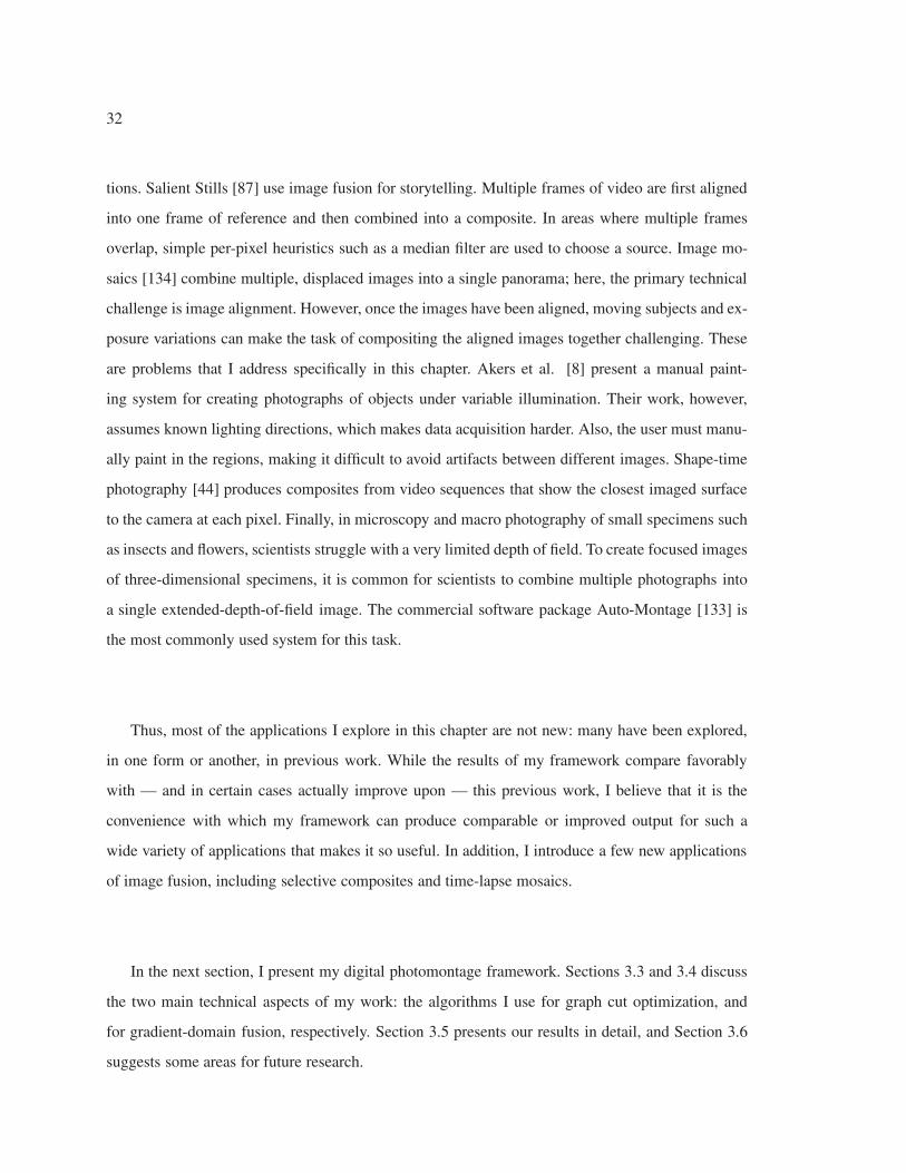
32

tions. Salient Stills [87] use image fusion for storytelling. Multiple frames of video are first aligned

into one frame of reference and then combined into a composite. In areas where multiple frames

overlap, simple per-pixel heuristics such as a median filter are used to choose a source. Image mo-

saics [134] combine multiple, displaced images into a single panorama; here, the primary technical

challenge is image alignment. However, once the images have been aligned, moving subjects and ex-

posure variations can make the task of compositing the aligned images together challenging. These

are problems that I address specifically in this chapter. Akers et al. [8] present a manual paint-

ing system for creating photographs of objects under variable illumination. Their work, however,

assumes known lighting directions, which makes data acquisition harder. Also, the user must manu-

ally paint in the regions, making it difficult to avoid artifacts between different images. Shape-time

photography [44] produces composites from video sequences that show the closest imaged surface

to the camera at each pixel. Finally, in microscopy and macro photography of small specimens such

as insects and flowers, scientists struggle with a very limited depth of field. To create focused images

of three-dimensional specimens, it is common for scientists to combine multiple photographs into

a single extended-depth-of-field image. The commercial software package Auto-Montage [133] is

the most commonly used system for this task.

Thus, most of the applications I explore in this chapter are not new: many have been explored,

in one form or another, in previous work. While the results of my framework compare favorably

with — and in certain cases actually improve upon — this previous work, I believe that it is the

convenience with which my framework can produce comparable or improved output for such a

wide variety of applications that makes it so useful. In addition, I introduce a few new applications

of image fusion, including selective composites and time-lapse mosaics.

In the next section, I present my digital photomontage framework. Sections 3.3 and 3.4 discuss

the two main technical aspects of my work: the algorithms I use for graph cut optimization, and

for gradient-domain fusion, respectively. Section 3.5 presents our results in detail, and Section 3.6

suggests some areas for future research.

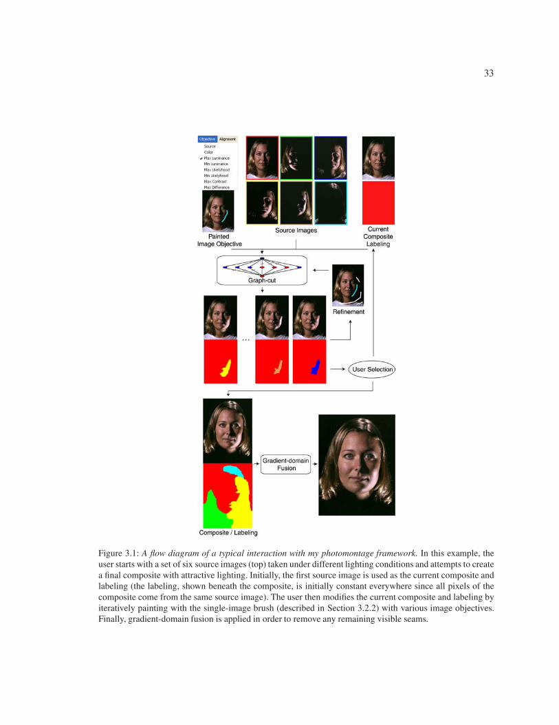
33

Figure 3.1: A flow diagram of a typical interaction with my photomontage framework. In this example, theuser starts with a set of six source images (top) taken under different lighting conditions and attempts to createa final composite with attractive lighting. Initially, the first source image is used as the current composite andlabeling (the labeling, shown beneath the composite, is initially constant everywhere since all pixels of thecomposite come from the same source image). The user then modifies the current composite and labeling byiteratively painting with the single-image brush (described in Section 3.2.2) with various image objectives.Finally, gradient-domain fusion is applied in order to remove any remaining visible seams.

34

3.2 The photomontage framework

The digital photomontage process begins with a set of source images, or image stack. For best

results, the source images should generally be related in some way. For instance, they might all be

of the same scene but with different lighting or camera positions. Or they might all be of a changing

scene, but with the camera locked down and the camera parameters fixed. When a static camera

is desired, the simplest approach is to use a tripod. Alternatively, in many cases the images can be

automatically aligned after the fact using one of a variety of previously published methods [134, 85].

My application interface makes use of two main windows: a source window, in which the user

can scroll through the source images; and a composite window, in which the user can see and interact

with the current result. New, intermediate results can also be added to the set of source images at

any time, in which case they can also be viewed in the source window and selected by the various

automatic algorithms about to be described.

Typically, the user goes through an iterative refinement process to create a composite. Associated

with the composite is a labeling, which is an array that specifies the source image for each pixel in

the composite.

3.2.1 Objectives

After loading a stack, the user can select an image objective that can be applied globally to the entire

image or locally to only a few pixels through a “painting”-style interface. The image objective at

each pixel specifies a property that the user would like to see at each pixel in the designated area of

the composite (or the entire composite, if it is specified globally). The image objective is computed

independently at each pixel position p, based on the set of pixel values drawn from that same position

p in each of the source images. I denote this set the span at each pixel.

The general image objectives that may be applied in a variety of applications include:

• Designated color: a specific desired color to either match or avoid (Figures 3.7 and 3.6).

• Minimum or maximum luminance: the darkest or lightest pixel in the span (Figures 3.7

and 3.6).

35

• Minimum or maximum contrast: the pixel from the span with the lowest or highest local

contrast in the span (Figures 3.8 and 3.11).

• Minimum or maximum likelihood: the least or most common pixel value in the span (subject

to a particular histogram quantization function, Figures 3.12 and 3.10).

• Eraser: the color most different from that of the current composite (Figure 3.10).

• Minimum or maximum difference: the color least or most similar to the color at position p

of a specific source image in the stack (Figure 3.12).

• Designated image: a specific source image in the stack (Figures 3.2, 3.12, 3.4, and 3.5).

For some photomontage applications I design custom image objectives (e.g., Figures 3.13 and

3.9). There is also a second type of objective that can be specified by the user, which I call a seam

objective. The seam objective measures the suitability of a seam between two image regions. Un-

like the image objective, it is always specified globally across the entire image. The types of seam

objectives I have implemented include:

• Colors: match colors across seams (Figures 3.12, 3.4, and 3.5).

• Colors & gradients: match colors and color gradients across seams (Figures 3.8, 3.13, 3.9, 3.11,

and 3.10).

• Colors & edges: match colors across seams, but prefer seams that lie along edges (Fig-

ures 3.2, 3.7, and 3.6).

The designated image objective was originally introduced by Kwatra et al. [77] to interactively

merge image regions. Many of the other objectives that I introduce do not require the selection of a

specific source, thus allowing the user to specify high-level goals for which the system automatically

selects the most appropriate sources. The colors and colors & edges seam objectives were also

introduced by Kwatra et al. .

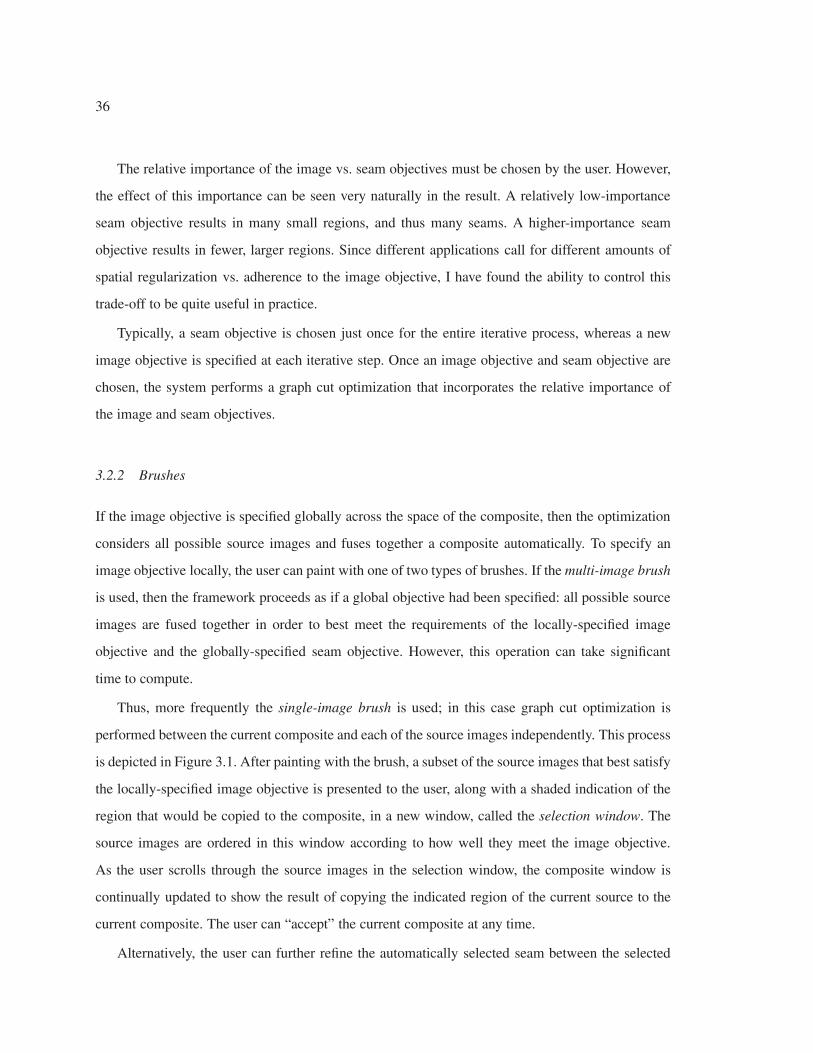
36

The relative importance of the image vs. seam objectives must be chosen by the user. However,

the effect of this importance can be seen very naturally in the result. A relatively low-importance

seam objective results in many small regions, and thus many seams. A higher-importance seam

objective results in fewer, larger regions. Since different applications call for different amounts of

spatial regularization vs. adherence to the image objective, I have found the ability to control this

trade-off to be quite useful in practice.

Typically, a seam objective is chosen just once for the entire iterative process, whereas a new

image objective is specified at each iterative step. Once an image objective and seam objective are

chosen, the system performs a graph cut optimization that incorporates the relative importance of

the image and seam objectives.

3.2.2 Brushes

If the image objective is specified globally across the space of the composite, then the optimization

considers all possible source images and fuses together a composite automatically. To specify an

image objective locally, the user can paint with one of two types of brushes. If the multi-image brush

is used, then the framework proceeds as if a global objective had been specified: all possible source

images are fused together in order to best meet the requirements of the locally-specified image

objective and the globally-specified seam objective. However, this operation can take significant

time to compute.

Thus, more frequently the single-image brush is used; in this case graph cut optimization is

performed between the current composite and each of the source images independently. This process

is depicted in Figure 3.1. After painting with the brush, a subset of the source images that best satisfy

the locally-specified image objective is presented to the user, along with a shaded indication of the

region that would be copied to the composite, in a new window, called the selection window. The

source images are ordered in this window according to how well they meet the image objective.

As the user scrolls through the source images in the selection window, the composite window is

continually updated to show the result of copying the indicated region of the current source to the

current composite. The user can “accept” the current composite at any time.

Alternatively, the user can further refine the automatically selected seam between the selected

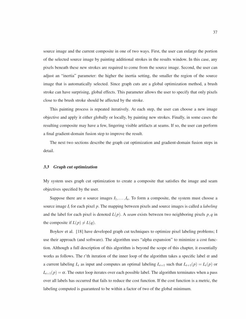
37

source image and the current composite in one of two ways. First, the user can enlarge the portion

of the selected source image by painting additional strokes in the results window. In this case, any

pixels beneath these new strokes are required to come from the source image. Second, the user can

adjust an “inertia” parameter: the higher the inertia setting, the smaller the region of the source

image that is automatically selected. Since graph cuts are a global optimization method, a brush

stroke can have surprising, global effects. This parameter allows the user to specify that only pixels

close to the brush stroke should be affected by the stroke.

This painting process is repeated iteratively. At each step, the user can choose a new image

objective and apply it either globally or locally, by painting new strokes. Finally, in some cases the

resulting composite may have a few, lingering visible artifacts at seams. If so, the user can perform

a final gradient-domain fusion step to improve the result.

The next two sections describe the graph cut optimization and gradient-domain fusion steps in

detail.

3.3 Graph cut optimization

My system uses graph cut optimization to create a composite that satisfies the image and seam

objectives specified by the user.

Suppose there are n source images I1, . . . , In. To form a composite, the system must choose a

source image Ii for each pixel p. The mapping between pixels and source images is called a labeling

and the label for each pixel is denoted L(p). A seam exists between two neighboring pixels p,q in

the composite if L(p) �= L(q).

Boykov et al. [18] have developed graph cut techniques to optimize pixel labeling problems; I

use their approach (and software). The algorithm uses “alpha expansion” to minimize a cost func-

tion. Although a full description of this algorithm is beyond the scope of this chapter, it essentially

works as follows. The t’th iteration of the inner loop of the algorithm takes a specific label α and

a current labeling Lt as input and computes an optimal labeling Lt+1 such that Lt+1(p) = Lt(p) or

Lt+1(p) = α . The outer loop iterates over each possible label. The algorithm terminates when a pass

over all labels has occurred that fails to reduce the cost function. If the cost function is a metric, the

labeling computed is guaranteed to be within a factor of two of the global minimum.

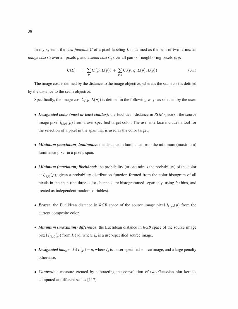
38

In my system, the cost function C of a pixel labeling L is defined as the sum of two terms: an

image cost Ci over all pixels p and a seam cost Cs over all pairs of neighboring pixels p,q:

C(L) = ∑p

Ci(p, L(p)) + ∑p,q

Cs(p, q, L(p), L(q)) (3.1)

The image cost is defined by the distance to the image objective, whereas the seam cost is defined

by the distance to the seam objective.

Specifically, the image cost Ci(p, L(p)) is defined in the following ways as selected by the user:

• Designated color (most or least similar): the Euclidean distance in RGB space of the source

image pixel IL(p)(p) from a user-specified target color. The user interface includes a tool for

the selection of a pixel in the span that is used as the color target.

• Minimum (maximum) luminance: the distance in luminance from the minimum (maximum)

luminance pixel in a pixels span.

• Minimum (maximum) likelihood: the probability (or one minus the probability) of the color

at IL(p)(p), given a probability distribution function formed from the color histogram of all

pixels in the span (the three color channels are histogrammed separately, using 20 bins, and

treated as independent random variables).

• Eraser: the Euclidean distance in RGB space of the source image pixel IL(p)(p) from the

current composite color.

• Minimum (maximum) difference: the Euclidean distance in RGB space of the source image

pixel IL(p)(p) from Iu(p), where Iu is a user-specified source image.

• Designated image: 0 if L(p) = u, where Iu is a user-specified source image, and a large penalty

otherwise.

• Contrast: a measure created by subtracting the convolution of two Gaussian blur kernels

computed at different scales [117].

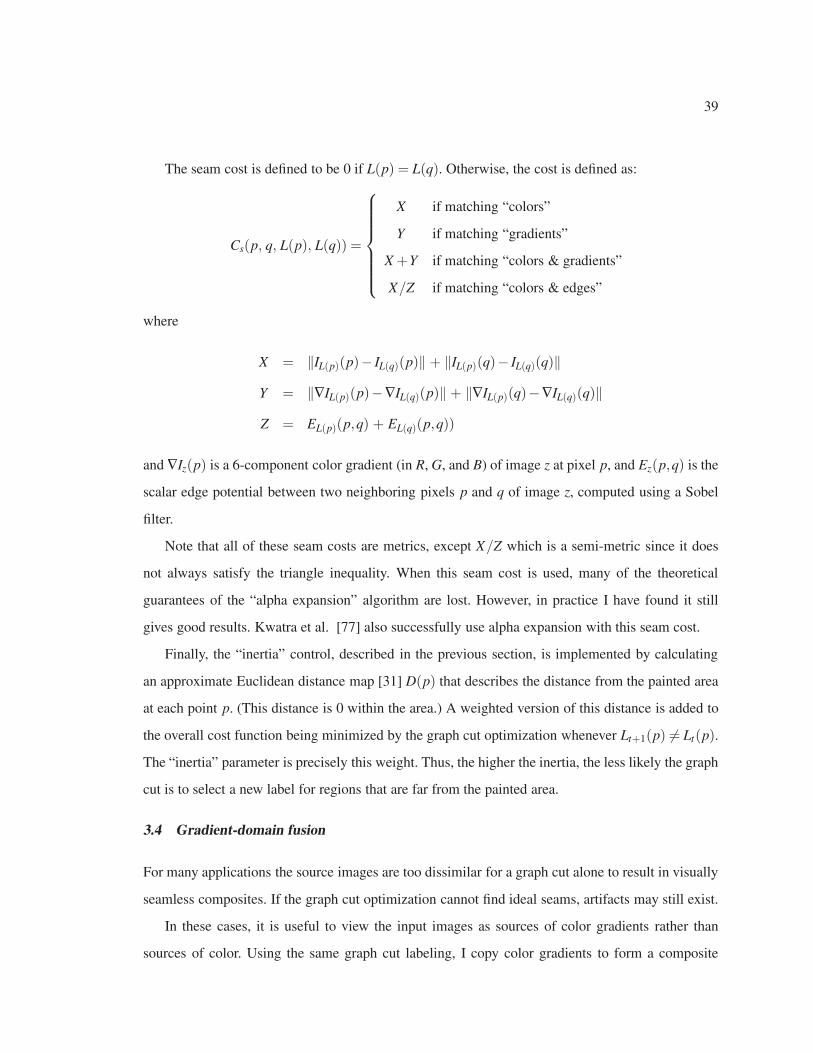
39

The seam cost is defined to be 0 if L(p) = L(q). Otherwise, the cost is defined as:

Cs(p, q, L(p), L(q)) =

⎧⎪⎪⎪⎪⎪⎪⎨⎪⎪⎪⎪⎪⎪⎩

X if matching “colors”

Y if matching “gradients”

X +Y if matching “colors & gradients”

X/Z if matching “colors & edges”

where

X = ‖IL(p)(p)− IL(q)(p)‖ + ‖IL(p)(q)− IL(q)(q)‖Y = ‖∇IL(p)(p)−∇IL(q)(p)‖ + ‖∇IL(p)(q)−∇IL(q)(q)‖Z = EL(p)(p,q) + EL(q)(p,q))

and ∇Iz(p) is a 6-component color gradient (in R, G, and B) of image z at pixel p, and Ez(p,q) is the

scalar edge potential between two neighboring pixels p and q of image z, computed using a Sobel

filter.

Note that all of these seam costs are metrics, except X/Z which is a semi-metric since it does

not always satisfy the triangle inequality. When this seam cost is used, many of the theoretical

guarantees of the “alpha expansion” algorithm are lost. However, in practice I have found it still

gives good results. Kwatra et al. [77] also successfully use alpha expansion with this seam cost.

Finally, the “inertia” control, described in the previous section, is implemented by calculating

an approximate Euclidean distance map [31] D(p) that describes the distance from the painted area

at each point p. (This distance is 0 within the area.) A weighted version of this distance is added to

the overall cost function being minimized by the graph cut optimization whenever Lt+1(p) �= Lt(p).

The “inertia” parameter is precisely this weight. Thus, the higher the inertia, the less likely the graph

cut is to select a new label for regions that are far from the painted area.

3.4 Gradient-domain fusion

For many applications the source images are too dissimilar for a graph cut alone to result in visually

seamless composites. If the graph cut optimization cannot find ideal seams, artifacts may still exist.

In these cases, it is useful to view the input images as sources of color gradients rather than

sources of color. Using the same graph cut labeling, I copy color gradients to form a composite

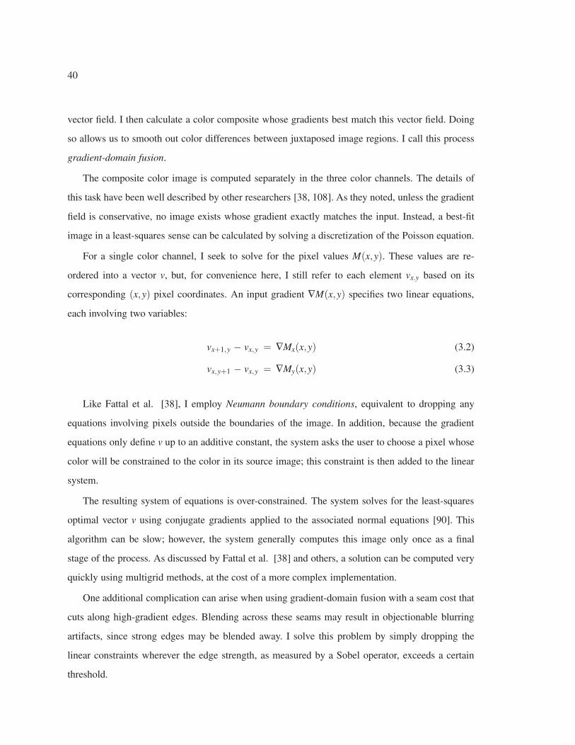
40

vector field. I then calculate a color composite whose gradients best match this vector field. Doing

so allows us to smooth out color differences between juxtaposed image regions. I call this process

gradient-domain fusion.

The composite color image is computed separately in the three color channels. The details of

this task have been well described by other researchers [38, 108]. As they noted, unless the gradient

field is conservative, no image exists whose gradient exactly matches the input. Instead, a best-fit

image in a least-squares sense can be calculated by solving a discretization of the Poisson equation.

For a single color channel, I seek to solve for the pixel values M(x,y). These values are re-

ordered into a vector v, but, for convenience here, I still refer to each element vx.y based on its

corresponding (x,y) pixel coordinates. An input gradient ∇M(x,y) specifies two linear equations,

each involving two variables:

vx+1,y − vx,y = ∇Mx(x,y) (3.2)

vx,y+1 − vx,y = ∇My(x,y) (3.3)

Like Fattal et al. [38], I employ Neumann boundary conditions, equivalent to dropping any

equations involving pixels outside the boundaries of the image. In addition, because the gradient

equations only define v up to an additive constant, the system asks the user to choose a pixel whose

color will be constrained to the color in its source image; this constraint is then added to the linear

system.

The resulting system of equations is over-constrained. The system solves for the least-squares

optimal vector v using conjugate gradients applied to the associated normal equations [90]. This

algorithm can be slow; however, the system generally computes this image only once as a final

stage of the process. As discussed by Fattal et al. [38] and others, a solution can be computed very

quickly using multigrid methods, at the cost of a more complex implementation.

One additional complication can arise when using gradient-domain fusion with a seam cost that

cuts along high-gradient edges. Blending across these seams may result in objectionable blurring

artifacts, since strong edges may be blended away. I solve this problem by simply dropping the

linear constraints wherever the edge strength, as measured by a Sobel operator, exceeds a certain

threshold.

41

3.5 Results

I now demonstrate how my system can be applied to a variety of tasks. Depending on the specific

task, a different set of image and seam objectives will be used to achieve the goal. Some results

(Figures 3.8, 3.13, 3.9,and 3.11) do not require painting by the user; they are computed automat-

ically by applying an image objective globally over the whole image. Other results are created by

user-painted image objectives (Figures 3.2, 3.7, 3.4, 3.5, and 3.6). Finally, the user may choose to

begin with a globally-computed composite, and then interactively modify it (Figures 3.12 and 3.10).

Selective composites. Photomontage allows us to interactively select and assemble the best frag-

ments of a set of images. Photographs of a group of people are a good example; it is difficult to

capture a group portrait without a few closed eyes or awkward expressions. In Figure 3.2, I merge

several group portraits into one that is better than any of the originals. Even portraiture of a single

person can be challenging and can be aided by assembling a composite (Figure 3.4). I can also push

the photomontage paradigm to create entirely fictional but surprisingly realistic (and sometimes

funny) composite portraits of different people (Figures 3.4 and 3.5).

Image-based relighting. Photography is the art of painting with light; my next application of

photomontage demonstrates this point. Studio portraiture (Figure 3.6) and product photography

(Figure 3.7) typically involve a complex lighting setup. Instead, I allow a user to literally paint

light, and simulate complex lighting with just a few brush strokes. After capturing a set of images

taken under various lighting conditions, I quickly relight a subject, both with realistic and non-

physically realizable lighting. This allows photographers to experiment with a wide range of lighting

possibilities after a shoot, instead of carefully planning a desired effect in advance. Note that several

of the image objectives can be thought of as highlight or shadow brushes that indicate the desired

placement of these lighting effects in a scene. The user can paint with the color image objective

using a bright, highlight color or a dark, shadow color to find highlights or shadows in a specific

location in the set of source images. Alternatively, the maximum or minimum luminance objectives

can also be used to find highlights or shadows, respectively, and add them to the composite.

Extended depth-of-field. In microscopy and macro photography of small specimens such as

insects and flowers, scientists struggle with a very limited depth of field. To create focused images

of three-dimensional specimens, it is common for scientists to combine multiple photographs into

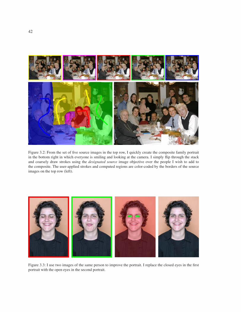
42

Figure 3.2: From the set of five source images in the top row, I quickly create the composite family portraitin the bottom right in which everyone is smiling and looking at the camera. I simply flip through the stackand coarsely draw strokes using the designated source image objective over the people I wish to add tothe composite. The user-applied strokes and computed regions are color-coded by the borders of the sourceimages on the top row (left).

Figure 3.3: I use two images of the same person to improve the portrait. I replace the closed eyes in the firstportrait with the open eyes in the second portrait.

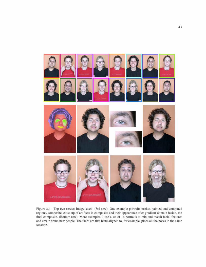
43

Figure 3.4: (Top two rows): Image stack. (3rd row): One example portrait: strokes painted and computedregions, composite, close-up of artifacts in composite and their appearance after gradient-domain fusion, thefinal composite. (Bottom row): More examples. I use a set of 16 portraits to mix and match facial featuresand create brand new people. The faces are first hand aligned to, for example, place all the noses in the samelocation.

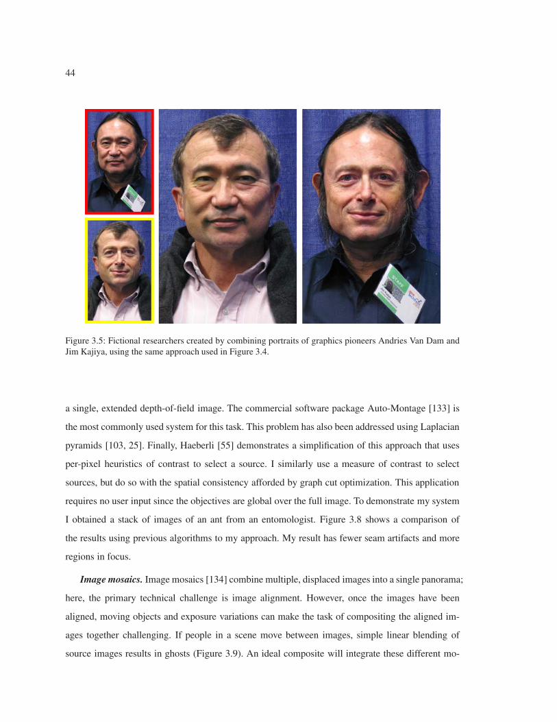
44

Figure 3.5: Fictional researchers created by combining portraits of graphics pioneers Andries Van Dam andJim Kajiya, using the same approach used in Figure 3.4.

a single, extended depth-of-field image. The commercial software package Auto-Montage [133] is

the most commonly used system for this task. This problem has also been addressed using Laplacian

pyramids [103, 25]. Finally, Haeberli [55] demonstrates a simplification of this approach that uses

per-pixel heuristics of contrast to select a source. I similarly use a measure of contrast to select

sources, but do so with the spatial consistency afforded by graph cut optimization. This application

requires no user input since the objectives are global over the full image. To demonstrate my system

I obtained a stack of images of an ant from an entomologist. Figure 3.8 shows a comparison of

the results using previous algorithms to my approach. My result has fewer seam artifacts and more

regions in focus.

Image mosaics. Image mosaics [134] combine multiple, displaced images into a single panorama;

here, the primary technical challenge is image alignment. However, once the images have been

aligned, moving objects and exposure variations can make the task of compositing the aligned im-

ages together challenging. If people in a scene move between images, simple linear blending of

source images results in ghosts (Figure 3.9). An ideal composite will integrate these different mo-

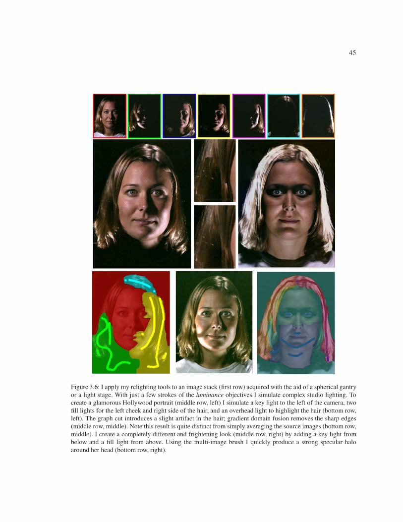
45

Figure 3.6: I apply my relighting tools to an image stack (first row) acquired with the aid of a spherical gantryor a light stage. With just a few strokes of the luminance objectives I simulate complex studio lighting. Tocreate a glamorous Hollywood portrait (middle row, left) I simulate a key light to the left of the camera, twofill lights for the left cheek and right side of the hair, and an overhead light to highlight the hair (bottom row,left). The graph cut introduces a slight artifact in the hair; gradient domain fusion removes the sharp edges(middle row, middle). Note this result is quite distinct from simply averaging the source images (bottom row,middle). I create a completely different and frightening look (middle row, right) by adding a key light frombelow and a fill light from above. Using the multi-image brush I quickly produce a strong specular haloaround her head (bottom row, right).

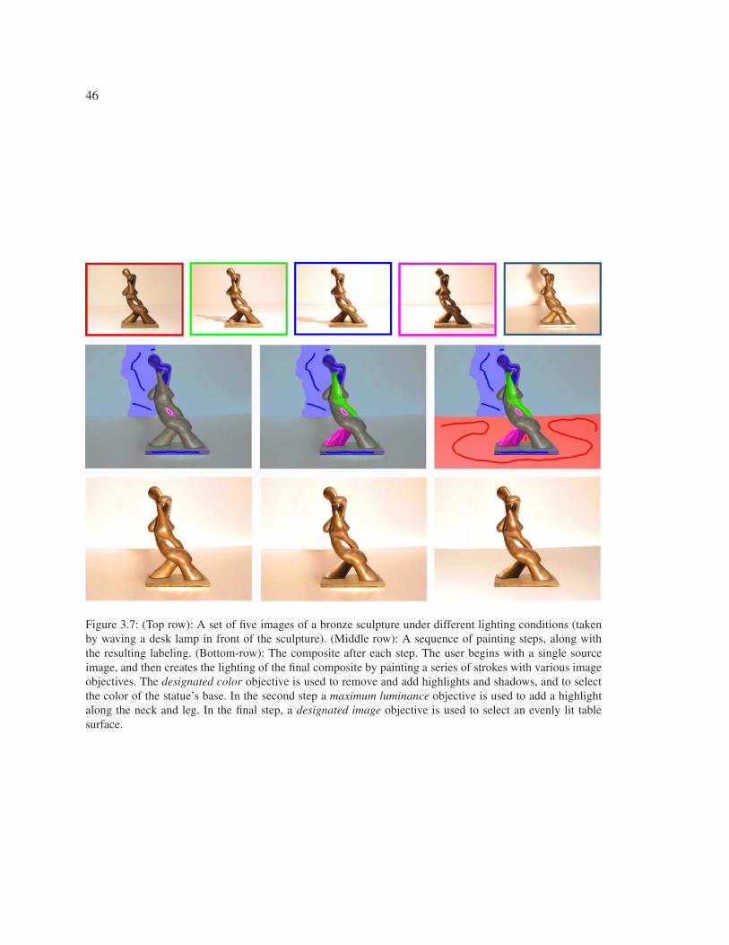
46

Figure 3.7: (Top row): A set of five images of a bronze sculpture under different lighting conditions (takenby waving a desk lamp in front of the sculpture). (Middle row): A sequence of painting steps, along withthe resulting labeling. (Bottom-row): The composite after each step. The user begins with a single sourceimage, and then creates the lighting of the final composite by painting a series of strokes with various imageobjectives. The designated color objective is used to remove and add highlights and shadows, and to selectthe color of the statue’s base. In the second step a maximum luminance objective is used to add a highlightalong the neck and leg. In the final step, a designated image objective is used to select an evenly lit tablesurface.

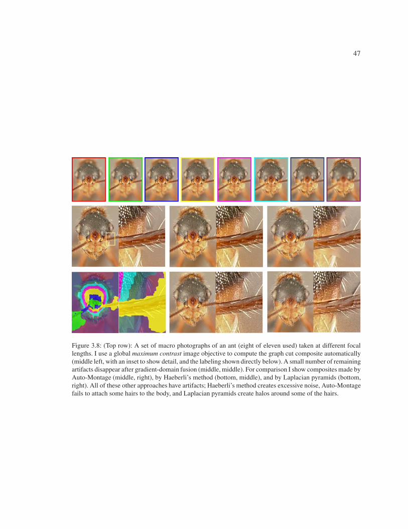
47

Figure 3.8: (Top row): A set of macro photographs of an ant (eight of eleven used) taken at different focallengths. I use a global maximum contrast image objective to compute the graph cut composite automatically(middle left, with an inset to show detail, and the labeling shown directly below). A small number of remainingartifacts disappear after gradient-domain fusion (middle, middle). For comparison I show composites made byAuto-Montage (middle, right), by Haeberli’s method (bottom, middle), and by Laplacian pyramids (bottom,right). All of these other approaches have artifacts; Haeberli’s method creates excessive noise, Auto-Montagefails to attach some hairs to the body, and Laplacian pyramids create halos around some of the hairs.

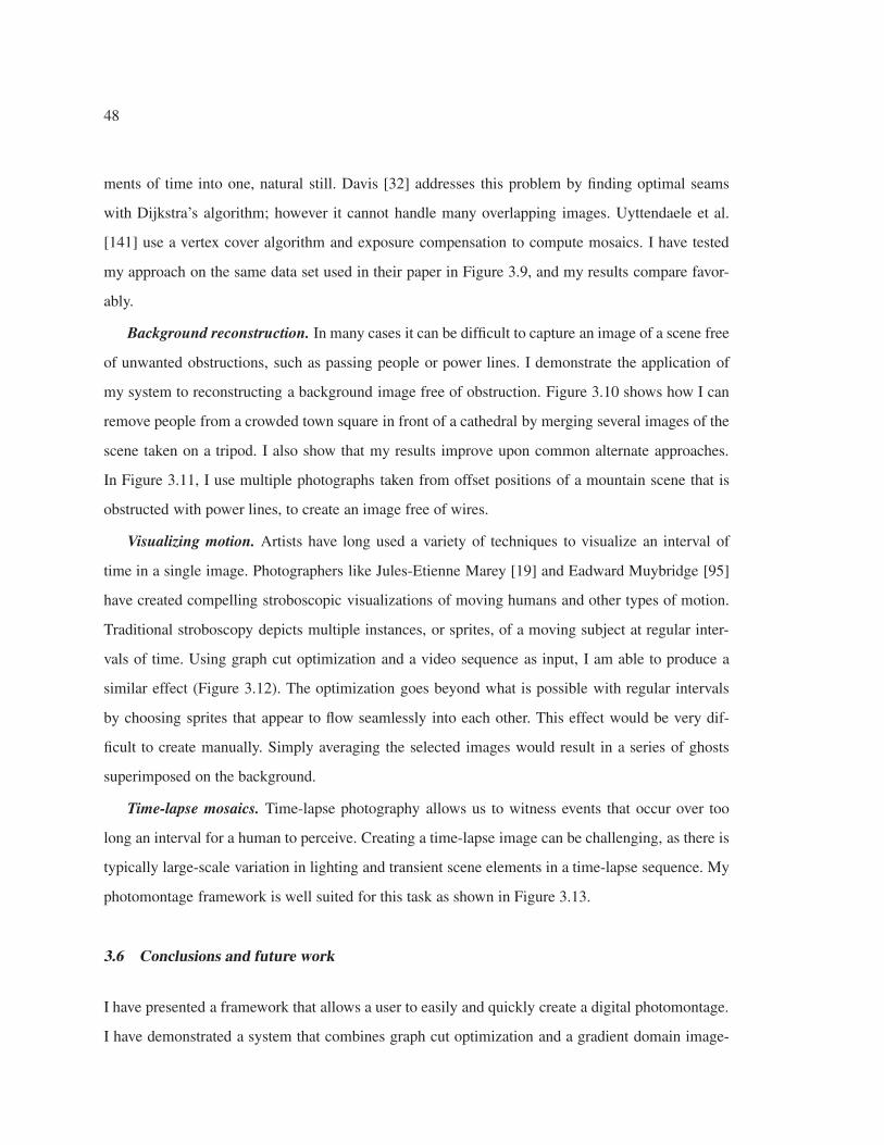
48

ments of time into one, natural still. Davis [32] addresses this problem by finding optimal seams

with Dijkstra’s algorithm; however it cannot handle many overlapping images. Uyttendaele et al.

[141] use a vertex cover algorithm and exposure compensation to compute mosaics. I have tested

my approach on the same data set used in their paper in Figure 3.9, and my results compare favor-

ably.

Background reconstruction. In many cases it can be difficult to capture an image of a scene free

of unwanted obstructions, such as passing people or power lines. I demonstrate the application of

my system to reconstructing a background image free of obstruction. Figure 3.10 shows how I can

remove people from a crowded town square in front of a cathedral by merging several images of the

scene taken on a tripod. I also show that my results improve upon common alternate approaches.

In Figure 3.11, I use multiple photographs taken from offset positions of a mountain scene that is

obstructed with power lines, to create an image free of wires.

Visualizing motion. Artists have long used a variety of techniques to visualize an interval of

time in a single image. Photographers like Jules-Etienne Marey [19] and Eadward Muybridge [95]

have created compelling stroboscopic visualizations of moving humans and other types of motion.

Traditional stroboscopy depicts multiple instances, or sprites, of a moving subject at regular inter-

vals of time. Using graph cut optimization and a video sequence as input, I am able to produce a

similar effect (Figure 3.12). The optimization goes beyond what is possible with regular intervals

by choosing sprites that appear to flow seamlessly into each other. This effect would be very dif-

ficult to create manually. Simply averaging the selected images would result in a series of ghosts

superimposed on the background.

Time-lapse mosaics. Time-lapse photography allows us to witness events that occur over too

long an interval for a human to perceive. Creating a time-lapse image can be challenging, as there is

typically large-scale variation in lighting and transient scene elements in a time-lapse sequence. My

photomontage framework is well suited for this task as shown in Figure 3.13.

3.6 Conclusions and future work

I have presented a framework that allows a user to easily and quickly create a digital photomontage.

I have demonstrated a system that combines graph cut optimization and a gradient domain image-

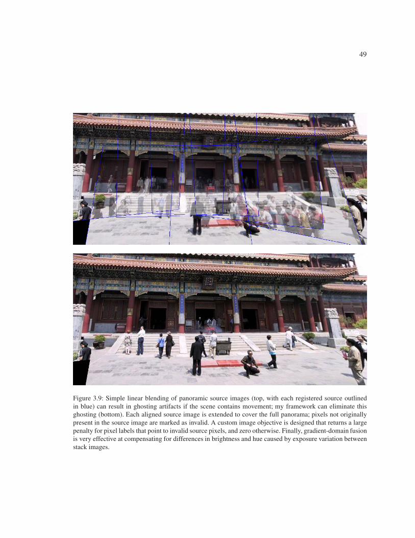
49

Figure 3.9: Simple linear blending of panoramic source images (top, with each registered source outlinedin blue) can result in ghosting artifacts if the scene contains movement; my framework can eliminate thisghosting (bottom). Each aligned source image is extended to cover the full panorama; pixels not originallypresent in the source image are marked as invalid. A custom image objective is designed that returns a largepenalty for pixel labels that point to invalid source pixels, and zero otherwise. Finally, gradient-domain fusionis very effective at compensating for differences in brightness and hue caused by exposure variation betweenstack images.

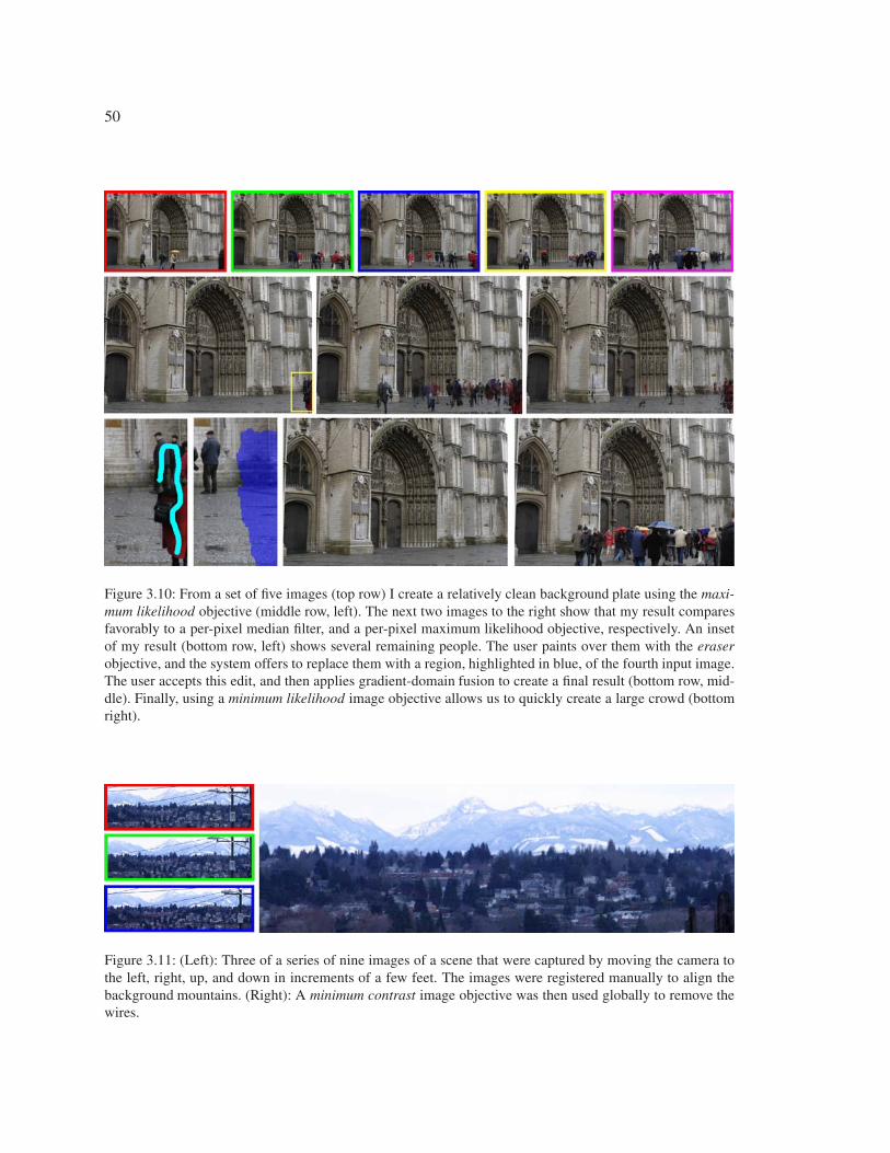
50

Figure 3.10: From a set of five images (top row) I create a relatively clean background plate using the maxi-mum likelihood objective (middle row, left). The next two images to the right show that my result comparesfavorably to a per-pixel median filter, and a per-pixel maximum likelihood objective, respectively. An insetof my result (bottom row, left) shows several remaining people. The user paints over them with the eraserobjective, and the system offers to replace them with a region, highlighted in blue, of the fourth input image.The user accepts this edit, and then applies gradient-domain fusion to create a final result (bottom row, mid-dle). Finally, using a minimum likelihood image objective allows us to quickly create a large crowd (bottomright).

Figure 3.11: (Left): Three of a series of nine images of a scene that were captured by moving the camera tothe left, right, up, and down in increments of a few feet. The images were registered manually to align thebackground mountains. (Right): A minimum contrast image objective was then used globally to remove thewires.

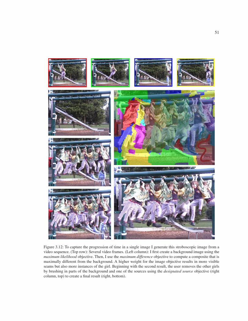
51

Figure 3.12: To capture the progression of time in a single image I generate this stroboscopic image from avideo sequence. (Top row): Several video frames. (Left column): I first create a background image using themaximum likelihood objective. Then, I use the maximum difference objective to compute a composite that ismaximally different from the background. A higher weight for the image objective results in more visibleseams but also more instances of the girl. Beginning with the second result, the user removes the other girlsby brushing in parts of the background and one of the sources using the designated source objective (rightcolumn, top) to create a final result (right, bottom).

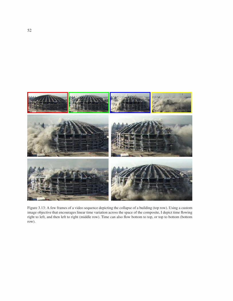
52

Figure 3.13: A few frames of a video sequence depicting the collapse of a building (top row). Using a customimage objective that encourages linear time variation across the space of the composite, I depict time flowingright to left, and then left to right (middle row). Time can also flow bottom to top, or top to bottom (bottomrow).

53

fusion algorithm with an intuitive user interface for defining local and global objectives. My work

on digital photomontage suggests a number of areas for future work.

My system has been shown to be applicable to a wide range of photomontage applications;

however, I strongly suspect that there are many more. In the process of conducting this research I

have discovered that a surprising array of beautiful, useful, and unexpected images can arise from

an image stack. An exciting opportunity for future work is to discover more applications of pho-

tomontage. This would involve finding new types of image stacks than the ones presented here, and

possibly new image objectives that would be used to find the best parts of a stack to retain in a

composite.

Several of the applications I present require user guidance in selecting the best parts of im-

ages (e.g., image-based relighting and selective composites); more sophisticated image objectives

could be defined that automatically find the best parts of images. For example, the group portrait in

Figure 3.2 could created by automatically finding the best portrait of each person.

Finally, it may be possible to apply my approach to other types of data, such as 2.5D layered

images, video sequences, 3D volumes, or even polygonal models. Such data sets would probably

require new image and seam objectives that consider the relationships between the additional dimen-

sions of the data, and an interface for controlling optimization in these higher dimensional spaces.

54

Chapter 4

PHOTOGRAPHING LONG SCENES WITH MULTI-VIEWPOINT PANORAMAS

The photomontage system described in the previous chapter is mostly designed for creating

single-viewpoint composite images of a scene. The input images sample the plenoptic function

in a very constrained fashion; typically, the viewpoint is fixed by placing the camera on a tripod,

and the only variations between the input images occur over time. Over time there are changes

in scene properties (such as lighting or object positions) or camera parameters (such as the focal

plane). A slightly different scenario was shown in Figure 3.11, for which the camera position was

slightly shifted between each photograph. In this simple example, shifts in viewpoint were used to

remove power lines. There are other reasons, however, to create composite images that incorporate

multiple viewpoints; I surveyed some of these reasons in Section 2.2.1. In this chapter1 I extend

the photomontage approach to create composites from multiple viewpoints in order to effectively

visualize scenes that are too long to depict from any one viewpoint.

Imagine, for example, trying to take a photograph of all the buildings on one side of a city street

extending for several blocks. A single photograph from the street’s opposite side would capture

only a short portion of the scene. A photograph with a wider field of view would capture a slightly

longer section of the street, but the buildings would appear more and more distorted towards the

edges of the image. Another possibility would be to take a photograph from a faraway viewpoint.

Unfortunately, it is usually not possible to get far enough away from the side of a street in a dense

city to capture such a photograph. Even if one could get far enough way, the result would lose the

perspective depth cues that we see when walking down a street, such as awnings that get bigger as

they extend from buildings, and crossing streets that converge as they extend away from the viewer.

The problems described here are not unique to streets. In general, single-perspective photographs

are not very effective at conveying long scenes, such as the bank of a river or the aisle of a grocery

store. In this chapter I introduce a practical approach to producing panoramas that visualize these

1The work described in this chapter was originally presented as a paper [2] at SIGGRAPH 2006.

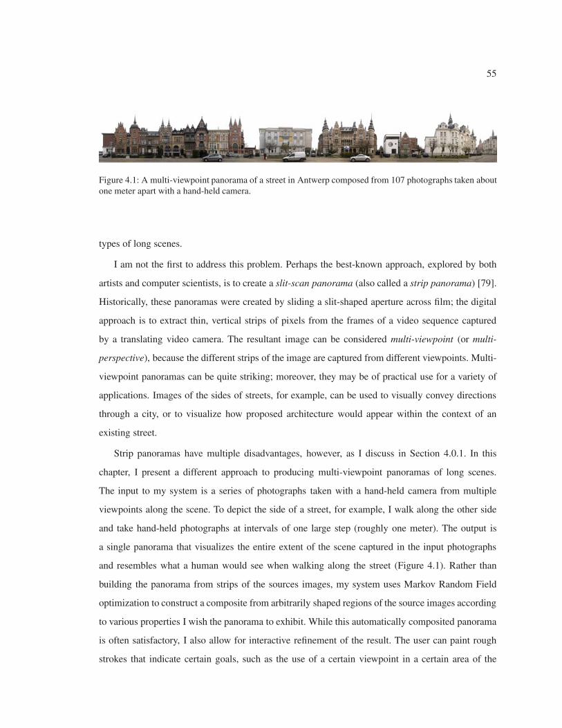
55

Figure 4.1: A multi-viewpoint panorama of a street in Antwerp composed from 107 photographs taken aboutone meter apart with a hand-held camera.

types of long scenes.

I am not the first to address this problem. Perhaps the best-known approach, explored by both

artists and computer scientists, is to create a slit-scan panorama (also called a strip panorama) [79].

Historically, these panoramas were created by sliding a slit-shaped aperture across film; the digital

approach is to extract thin, vertical strips of pixels from the frames of a video sequence captured

by a translating video camera. The resultant image can be considered multi-viewpoint (or multi-

perspective), because the different strips of the image are captured from different viewpoints. Multi-

viewpoint panoramas can be quite striking; moreover, they may be of practical use for a variety of

applications. Images of the sides of streets, for example, can be used to visually convey directions

through a city, or to visualize how proposed architecture would appear within the context of an

existing street.

Strip panoramas have multiple disadvantages, however, as I discuss in Section 4.0.1. In this

chapter, I present a different approach to producing multi-viewpoint panoramas of long scenes.

The input to my system is a series of photographs taken with a hand-held camera from multiple

viewpoints along the scene. To depict the side of a street, for example, I walk along the other side

and take hand-held photographs at intervals of one large step (roughly one meter). The output is

a single panorama that visualizes the entire extent of the scene captured in the input photographs

and resembles what a human would see when walking along the street (Figure 4.1). Rather than

building the panorama from strips of the sources images, my system uses Markov Random Field

optimization to construct a composite from arbitrarily shaped regions of the source images according

to various properties I wish the panorama to exhibit. While this automatically composited panorama

is often satisfactory, I also allow for interactive refinement of the result. The user can paint rough

strokes that indicate certain goals, such as the use of a certain viewpoint in a certain area of the

56

panorama. The major contribution of my work is a practical approach to creating high-quality, high-

resolution, multi-viewpoint panoramas with a simple and casual capture method. To accomplish this

goal, I present a number of novel techniques, including an objective function that describes desirable

properties of a multi-viewpoint panorama, and a novel technique for propagating user-drawn strokes

that annotate 3D objects in the scene (Section 4.1.4).

4.0.1 Related work

The term “panorama” typically refers to single-viewpoint panoramas, which can be created by

rotating a camera around its optical center [134]. Strip panoramas, however, are created from a

translating camera, and there are many variants, e.g., “pushbroom panoramas” [54, 128], “adaptive

manifolds” [107], and “x-slit” images [152]. Zheng [150] and Roman et al. [120] both describe

techniques designed specifically for creating strip panoramas of long streets.

In their simplest form, strip panoramas exhibit orthographic projection along the horizontal axis,

and perspective projection along the vertical. This disparity in projection leads to distortions for

scenes that are not strictly planar. Objects at a certain depth from the camera plane are shown

with a correct aspect ratio, but objects further from the camera appear horizontally stretched while

closer objects appear squashed. The depth at which objects are shown correctly can be adjusted

by varying the width of the strips taken from the video frames. Automatic approaches to varying

strip width either estimate scene depth [116] or attempt to minimize the appearance of vertical

seams [144]. Roman et al. [120] take an interactive approach. In their system, the user can choose

to include several separated strips of single-viewpoint perspective in the panorama; the system will

then interpolate viewpoints between these regions. They demonstrate better results than traditional

strip panoramas, but require a complex capture setup. Since they need a dense sampling of all rays

that intersect the camera path (i.e., a 3D light field), they use a high-speed 300-frame-per-second

video camera mounted on a truck that drives slowly down the street.

All of these variants of strip panoramas still exhibit distortions for scene with varying depths,

especially if these depth variations occur across the vertical axis of the image. There are other

problems with strip panoramas as well. The use of orthographic projection across the horizontal

axis of the image sacrifices local perspective effects that serve as useful depth cues; in the case of

57

a street, for example, crossing streets will not converge to a vanishing point as they extend away

from the viewer. Another problem is that strip panoramas are created from video sequences, and

still images created from video rarely have the same quality as those captured by a still camera. The

resolution is much lower, compression artifacts are usually noticeable, and noise is more prevalent

since a constantly moving video camera must use a short exposure to avoid motion blur. Finally,

capturing a suitable video can be cumbersome; strip panoramas are not typically created with a

hand-held video camera, for example.

Strip panoramas are not the only way to image in multiple perspectives. Multi-perspective imag-

ing can take many forms, from the more extreme non-photorealism of Cubism to the subtle depar-

tures from linear perspective often used by Renaissance artists [76] to achieve various properties

and arrangements in pictorial space. Several researchers have explored multi-perspective renderings

of 3D models [7, 148]. Yu and McMillan presented a model that can describe any multi-perspective

camera [149]. Multi-perspective images have also been used as a data structure to facilitate the

generation of traditional perspective views [147, 111, 152]. In the field of photogrammetry [69],

aerial or satellite imagery from varying viewpoints are stitched together to create near-orthographic,

top-down views of the earth (e.g., Google Earth [51]).

4.0.2 Approach

My approach to generating effective multi-viewpoint images is inspired by the work of artist Michael

Koller [73], who creates multi-viewpoint panoramas of San Francisco streets that consist of large

regions of ordinary perspective photographs artfully seamed together to hide the transitions (Fig-

ure 2.4). There is no obvious standard or ground truth by which to evaluate whether a specific

multi-viewpoint panorama visualizes a scene well, even if the 3D scene geometry and appearance

were known. Koller’s images, however, are attractive and informative, so I attempt to define some

of their properties:

1. Each object in the scene is rendered from a viewpoint roughly in front of it to avoid perspective

distortion.

2. The panoramas are composed of large regions of linear perspective seen from a viewpoint

58

where a person would naturally stand (for example, a city block is viewed from across the

street, rather than from some faraway viewpoint).

3. Local perspective effects are evident; objects closer to the image plane are larger than objects

further away, and multiple vanishing points can be seen.

4. The seams between these perspective regions do not draw attention; that is, the image appears

natural and continuous.

I thus designed my system to generate multi-viewpoint panoramas that exhibit these properties

as well as possible. Note, however, that maximizing these properties may not produce an effective

multi-viewpoint panorama for any arbitrary scene. Koller’s images are particularly good at visualiz-

ing certain types of scenes: those that are too long to effectively image from a single viewpoint, and

those whose geometry predominantly lies along a large, dominant plane (for example, the fronts of

the buildings in Figure 4.1). Because of this latter property, these scenes can be effectively visual-

ized by a single two-dimensional image whose image plane is parallel to the dominant plane of the

scene. More three-dimensional phenomena are unlikely to be well-summarized by a single image.

I have not, for example, attempted to create multi-viewpoint panoramas that turn around street cor-

ners, or that show all four sides of a building, since they are likely to be less comprehensible to the

average viewer. Note also that the dominant plane need not be strictly planar. For example, the river

bank I depict in Figure 4.13 curves significantly (as is evident from the plan view in Figure 4.5).

My system requires the user to specify a picture surface that lies along the dominant plane. The

system’s success depends on a key observation (see Figure 4.2): images projected onto the picture

surface from their original 3D viewpoints will agree in areas depicting scene geometry lying on the

dominant plane (assuming Lambertian reflectance and the absence of occlusions). This agreement

can be visualized by averaging the projections of all of the cameras onto the picture surface (Fig-

ure 4.7). The resulting image is sharp for geometry near the dominant plane because these projec-

tions are consistent and blurry for objects at other depths.2 Transitions between different viewpoints

can thus be placed in these aligned areas without causing objectionable artifacts. My system uses

2This image bears some resemblance to synthetic-aperture photography [80], though with much sparser sampling.

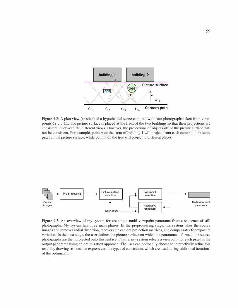
59

Figure 4.2: A plan view (xz slice) of a hypothetical scene captured with four photographs taken from view-points C1, . . . ,C4. The picture surface is placed at the front of the two buildings so that their projections areconsistent inbetween the different views. However, the projections of objects off of the picture surface willnot be consistent. For example, point a on the front of building 1 will project from each camera to the samepixel on the picture surface, while point b on the tree will project to different places.

Figure 4.3: An overview of my system for creating a multi-viewpoint panorama from a sequence of stillphotographs. My system has three main phases. In the preprocessing stage, my system takes the sourceimages and removes radial distortion, recovers the camera projection matrices, and compensates for exposurevariation. In the next stage, the user defines the picture surface on which the panorama is formed; the sourcephotographs are then projected onto this surface. Finally, my system selects a viewpoint for each pixel in theoutput panorama using an optimization approach. The user can optionally choose to interactively refine thisresult by drawing strokes that express various types of constraints, which are used during additional iterationsof the optimization.

60

Markov Random Field optimization to choose one viewpoint for each pixel in the output panorama;

the optimization tries to place seams between viewpoints in aligned areas, while also maximizing

the four desirable properties of a multi-viewpoint panorama listed above.

The operating range of my approach is thus limited to scenes whose geometry intersects the

dominant plane often enough for natural transitions between viewpoints to occur. The required fre-

quency of these intersections varies inversely with the field of view of the input photographs, since

my approach is unlikely to work well if a portion of the scene larger than the field of view of one

camera is entirely off of the dominant plane. For this reason I often use a fisheye lens to insure a

wide field of view. My approach is not, however, limited to strictly planar scenes (which are trivial

to stitch). In fact, regions off of the dominant plane provide valuable local perspective cues that im-

prove the overall composition. My goal is to leave these areas intact and in their correct aspect ratios

(unlike strip panoramas, which squash or stretch regions off of the dominant plane). This goal can

be accomplished by restricting transitions between viewpoints to areas intersecting the dominant

plane. Objects off of the dominant plane will thus be either depicted entirely from one viewpoint, or

omitted altogether (by using viewpoints that see around the object, which generally works only for

small objects).

It is not always possible to limit transitions to areas intersecting the picture surface. For example,

the bottom of Figure 4.1 contains cars, sidewalk, and road, none of which lie near the picture surface

located at the front of the buildings. In this case, transitions between viewpoints must “cheat” and

splice together image regions that do not actually represent the same geometry. The transitions

between these image regions should be placed where they are least noticeable; for example, splicing

together separate regions of sidewalk in Figure 4.1 will likely not be objectionable. Such decisions,

however, are subjective and not always successful. I thus allow the user to easily refine the results

by drawing rough strokes indicating various constraints, as described in Section 4.1.4. The result in

Figure 4.1, however, required no interactive refinement.

4.1 System details

An overview of my system is shown in Figure 4.3. I now describe each step of my system in detail.

I begin by capturing a sequence of photographs that depict the scene for which I wish to produce

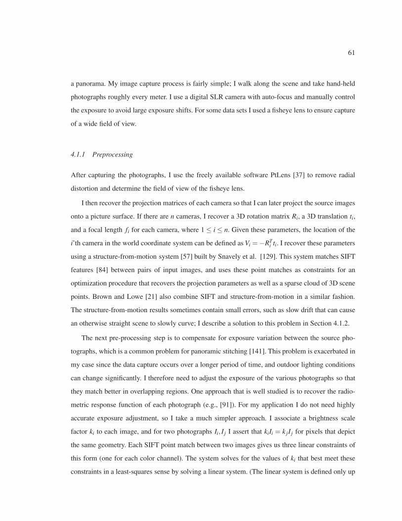
61

a panorama. My image capture process is fairly simple; I walk along the scene and take hand-held

photographs roughly every meter. I use a digital SLR camera with auto-focus and manually control

the exposure to avoid large exposure shifts. For some data sets I used a fisheye lens to ensure capture

of a wide field of view.

4.1.1 Preprocessing

After capturing the photographs, I use the freely available software PtLens [37] to remove radial

distortion and determine the field of view of the fisheye lens.

I then recover the projection matrices of each camera so that I can later project the source images

onto a picture surface. If there are n cameras, I recover a 3D rotation matrix Ri, a 3D translation ti,

and a focal length fi for each camera, where 1 ≤ i ≤ n. Given these parameters, the location of the

i’th camera in the world coordinate system can be defined as Vi = −RTi ti. I recover these parameters

using a structure-from-motion system [57] built by Snavely et al. [129]. This system matches SIFT

features [84] between pairs of input images, and uses these point matches as constraints for an

optimization procedure that recovers the projection parameters as well as a sparse cloud of 3D scene

points. Brown and Lowe [21] also combine SIFT and structure-from-motion in a similar fashion.

The structure-from-motion results sometimes contain small errors, such as slow drift that can cause

an otherwise straight scene to slowly curve; I describe a solution to this problem in Section 4.1.2.

The next pre-processing step is to compensate for exposure variation between the source pho-

tographs, which is a common problem for panoramic stitching [141]. This problem is exacerbated in

my case since the data capture occurs over a longer period of time, and outdoor lighting conditions

can change significantly. I therefore need to adjust the exposure of the various photographs so that

they match better in overlapping regions. One approach that is well studied is to recover the radio-

metric response function of each photograph (e.g., [91]). For my application I do not need highly

accurate exposure adjustment, so I take a much simpler approach. I associate a brightness scale

factor ki to each image, and for two photographs Ii, I j I assert that kiIi = k jI j for pixels that depict

the same geometry. Each SIFT point match between two images gives us three linear constraints of

this form (one for each color channel). The system solves for the values of ki that best meet these

constraints in a least-squares sense by solving a linear system. (The linear system is defined only up

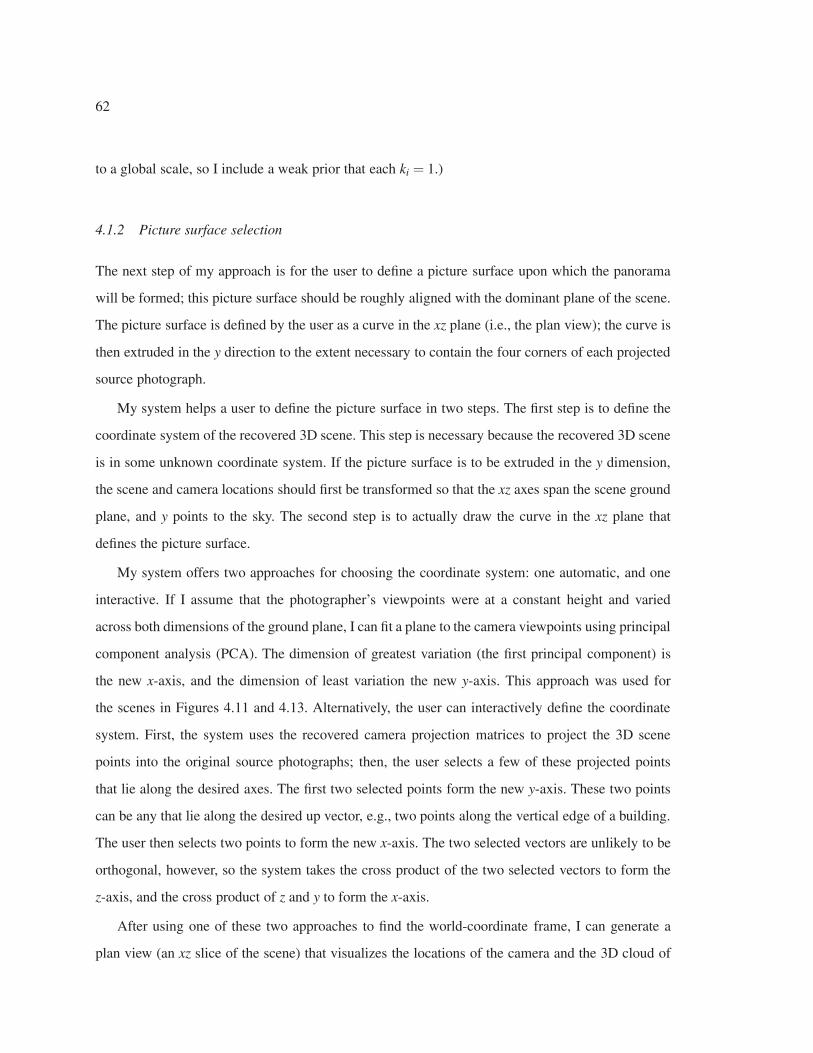
62

to a global scale, so I include a weak prior that each ki = 1.)

4.1.2 Picture surface selection

The next step of my approach is for the user to define a picture surface upon which the panorama

will be formed; this picture surface should be roughly aligned with the dominant plane of the scene.

The picture surface is defined by the user as a curve in the xz plane (i.e., the plan view); the curve is

then extruded in the y direction to the extent necessary to contain the four corners of each projected

source photograph.

My system helps a user to define the picture surface in two steps. The first step is to define the

coordinate system of the recovered 3D scene. This step is necessary because the recovered 3D scene

is in some unknown coordinate system. If the picture surface is to be extruded in the y dimension,

the scene and camera locations should first be transformed so that the xz axes span the scene ground

plane, and y points to the sky. The second step is to actually draw the curve in the xz plane that

defines the picture surface.

My system offers two approaches for choosing the coordinate system: one automatic, and one

interactive. If I assume that the photographer’s viewpoints were at a constant height and varied

across both dimensions of the ground plane, I can fit a plane to the camera viewpoints using principal

component analysis (PCA). The dimension of greatest variation (the first principal component) is

the new x-axis, and the dimension of least variation the new y-axis. This approach was used for

the scenes in Figures 4.11 and 4.13. Alternatively, the user can interactively define the coordinate

system. First, the system uses the recovered camera projection matrices to project the 3D scene

points into the original source photographs; then, the user selects a few of these projected points

that lie along the desired axes. The first two selected points form the new y-axis. These two points

can be any that lie along the desired up vector, e.g., two points along the vertical edge of a building.

The user then selects two points to form the new x-axis. The two selected vectors are unlikely to be

orthogonal, however, so the system takes the cross product of the two selected vectors to form the

z-axis, and the cross product of z and y to form the x-axis.

After using one of these two approaches to find the world-coordinate frame, I can generate a

plan view (an xz slice of the scene) that visualizes the locations of the camera and the 3D cloud of

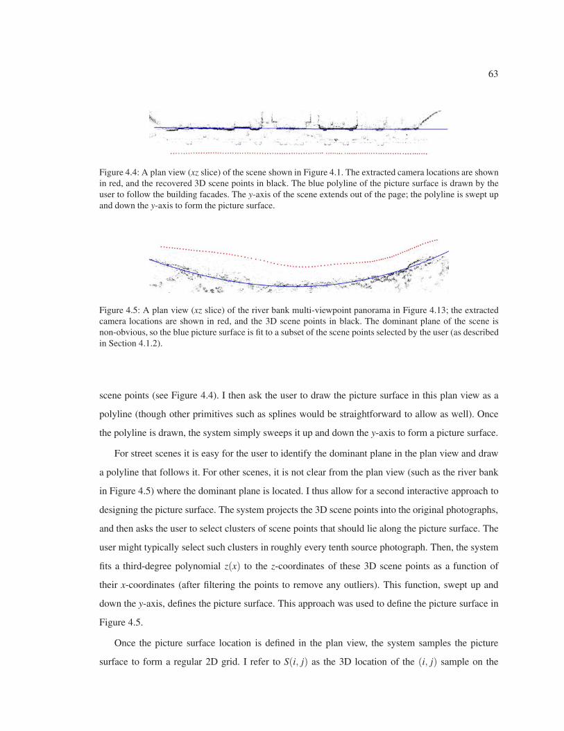
63

Figure 4.4: A plan view (xz slice) of the scene shown in Figure 4.1. The extracted camera locations are shownin red, and the recovered 3D scene points in black. The blue polyline of the picture surface is drawn by theuser to follow the building facades. The y-axis of the scene extends out of the page; the polyline is swept upand down the y-axis to form the picture surface.

Figure 4.5: A plan view (xz slice) of the river bank multi-viewpoint panorama in Figure 4.13; the extractedcamera locations are shown in red, and the 3D scene points in black. The dominant plane of the scene isnon-obvious, so the blue picture surface is fit to a subset of the scene points selected by the user (as describedin Section 4.1.2).

scene points (see Figure 4.4). I then ask the user to draw the picture surface in this plan view as a

polyline (though other primitives such as splines would be straightforward to allow as well). Once

the polyline is drawn, the system simply sweeps it up and down the y-axis to form a picture surface.

For street scenes it is easy for the user to identify the dominant plane in the plan view and draw

a polyline that follows it. For other scenes, it is not clear from the plan view (such as the river bank

in Figure 4.5) where the dominant plane is located. I thus allow for a second interactive approach to

designing the picture surface. The system projects the 3D scene points into the original photographs,

and then asks the user to select clusters of scene points that should lie along the picture surface. The

user might typically select such clusters in roughly every tenth source photograph. Then, the system

fits a third-degree polynomial z(x) to the z-coordinates of these 3D scene points as a function of

their x-coordinates (after filtering the points to remove any outliers). This function, swept up and

down the y-axis, defines the picture surface. This approach was used to define the picture surface in

Figure 4.5.

Once the picture surface location is defined in the plan view, the system samples the picture

surface to form a regular 2D grid. I refer to S(i, j) as the 3D location of the (i, j) sample on the

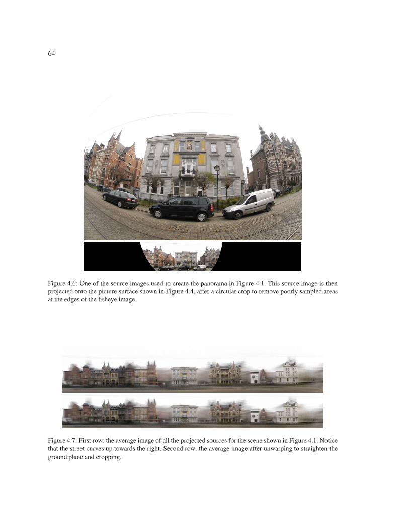
64

Figure 4.6: One of the source images used to create the panorama in Figure 4.1. This source image is thenprojected onto the picture surface shown in Figure 4.4, after a circular crop to remove poorly sampled areasat the edges of the fisheye image.

Figure 4.7: First row: the average image of all the projected sources for the scene shown in Figure 4.1. Noticethat the street curves up towards the right. Second row: the average image after unwarping to straighten theground plane and cropping.

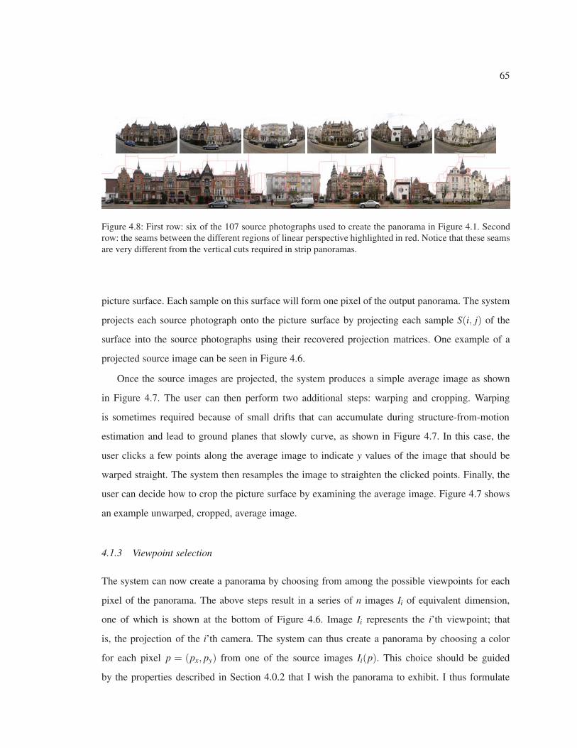
65

Figure 4.8: First row: six of the 107 source photographs used to create the panorama in Figure 4.1. Secondrow: the seams between the different regions of linear perspective highlighted in red. Notice that these seamsare very different from the vertical cuts required in strip panoramas.

picture surface. Each sample on this surface will form one pixel of the output panorama. The system

projects each source photograph onto the picture surface by projecting each sample S(i, j) of the

surface into the source photographs using their recovered projection matrices. One example of a

projected source image can be seen in Figure 4.6.

Once the source images are projected, the system produces a simple average image as shown

in Figure 4.7. The user can then perform two additional steps: warping and cropping. Warping

is sometimes required because of small drifts that can accumulate during structure-from-motion

estimation and lead to ground planes that slowly curve, as shown in Figure 4.7. In this case, the

user clicks a few points along the average image to indicate y values of the image that should be

warped straight. The system then resamples the image to straighten the clicked points. Finally, the

user can decide how to crop the picture surface by examining the average image. Figure 4.7 shows

an example unwarped, cropped, average image.

4.1.3 Viewpoint selection

The system can now create a panorama by choosing from among the possible viewpoints for each

pixel of the panorama. The above steps result in a series of n images Ii of equivalent dimension,

one of which is shown at the bottom of Figure 4.6. Image Ii represents the i’th viewpoint; that

is, the projection of the i’th camera. The system can thus create a panorama by choosing a color

for each pixel p = (px, py) from one of the source images Ii(p). This choice should be guided

by the properties described in Section 4.0.2 that I wish the panorama to exhibit. I thus formulate

66

an objective function that approximately measures these properties, and then minimize it using

Markov Random Field (MRF) optimization. As in chapter 3, the optimization computes a labeling

L(p), where L(p) = i if pixel p of the panorama is assigned color Ii(p). My objective function has

three terms, which I now describe.

The first term reflects the property that an object in the scene should be imaged from a viewpoint

roughly in front of it. The notion of “in front” depends on the orientation of the scene geometry, so

I use the picture surface as a proxy for this geometry. Consider a line that extends from a sample

of the picture surface S(p) in the direction of the normal to the picture surface at S(p). Any camera

viewpoint along this normal will be the most “in front,” or, put another way, will view the scene in

the most straight-on manner. I can thus evaluate this heuristic for a pixel p that chooses its color

from Ii by measuring the angle between the vector S(p)−Vi and the normal of the picture surface

at S(p). Note that the optical axis of the camera (i.e., the direction the camera is facing) is not used.

My system approximates this heuristic using a simpler and more computationally efficient method

that is accurate if the cameras are roughly the same distance from the picture surface. I find the pixel

pi whose corresponding 3D sample S(pi) on the picture surface is closest to camera location Vi; in

the case of a planar picture surface, this sample is exactly the sample for which camera Vi gives the

most straight-on view. Then, if pixel p chooses its color from Ii, I approximate the heuristic as the

2D distance from p to pi. Specifically, I define the cost function

Ci(p,L(p)) = |p− pL(p)|.

The second term of the objective function encourages transitions between different regions of linear

perspective to be natural and seamless. In the previous chapter I showed that a seamless transition

will minimize the seam cost

Cs(p,L(p),q,L(q)) = |IL(p)(p)− IL(q)(p)|2 + |IL(p)(q)− IL(q)(q)|2 (4.1)

between each pair of neighboring pixels p and q.

The third term of the objective function encourages the panorama to resemble the average image

in areas where the scene geometry intersects the picture surface. To some extent this resemblance

will occur naturally since there will typically be little variance between the different viewpoints in

these areas of the panorama. However, motion in the scene, specular highlights, occlusions, and

67

other such phenomena can detract from my goal of accurately visualizing scene geometry near the

dominant plane. I thus calculate the mean and standard deviation of each pixel in the panorama

among the various Ii in a robust fashion to discount outliers. I use a vector median filter [10]

computed across the three color channels as a robust mean, and the median absolute deviation

(MAD) [62] as a robust standard deviation. The MAD is calculated as the median L2 distance from

the median color. I refer to the median image as M(x,y) and the MAD as σ(x,y). Assuming that

image color channels vary from 0 to 255, I define the cost function

Cm(p,L(p)) =

⎧⎨⎩

|M(p)− IL(p)(p)| if σ(p) < 10

0 otherwise(4.2)

to minimize the difference between the median image and the image defined by the current labeling

for those pixels whose robust standard deviation is low. Note that this approach will fail to identify

cases where scene geometry at the picture surface is frequently occluded. A more complicated al-

ternative, which I hope to explore, would be to compute view-dependent information about which

pixels in which view lie along the dominant plane using multi-view stereo techniques [67].

Finally, I mention a constraint: any one camera has a limited field of view and will not project

to every pixel of the panorama (e.g., the black pixels in Figure 4.6). I encode pixels in image Ii to

which the i’th camera does not project as null, and do not allow L(p) = i if Ii(p) = null. I thus wish

to compute a panorama that minimizes the overall cost function

C(L) = ∑p

(αCi(p,L(p))+ βCm(p,L(p)))+∑p,q

Cs(p,L(p),q,L(q)),

which sums the three terms over each pixel p and each pair of neighboring pixels p and q. This cost

function has the familiar form of a Markov Random Field and can be minimized in several ways;

as in the previous chapter, I do so using graph cut optimization [74] in a series of alpha-expansion

moves [18]. I determine the weights experimentally and use the same values α = 100 and β = .25

for all the results used in this chapter. However, these weights have natural meanings that could be

exposed to the user. Higher values of α encourage pixels from more straight-on views at the expense

of more noticeable seams. Lower values of both α and β are more likely to remove objects off of

the dominant plane (such as power lines or cars, in the case of a street).

Two additional steps are required to finish the panorama. I first compute the panorama at a lower

resolution so that the MRF optimization can be computed in reasonable time (typically around

68

20 minutes). I then create higher-resolution versions using the hierarchical approach described in

section 5.3.6. Finally, some artifacts may still exist from exposure variations or areas where natural

seams do not exist. I thus composite the final panorama in the gradient domain (as described in

section 3.4) to smooth errors across these seams.

4.1.4 Interactive refinement

As described in Section 4.0.2, there is no guarantee that the user will like the transitions between

regions of linear perspective determined by the MRF optimization. I thus allow for high-level inter-

active control over the result; the user should be able to express desired changes to the panorama

without tedious manual editing of the exact seam locations. Also, the interaction metaphor should

be natural and intuitive, so in a manner similar to the photomontage system in the previous chapter,

I allow the user to draw various types of strokes that indicate user-desired constraints.

My system offers three types of strokes. “View selection” strokes allow a user to indicate that

a certain viewpoint should be used in a certain area of the panorama. A “seam suppression” stroke

indicates an object through which no seam should pass; I describe a novel technique for propagating

this stroke across the different positions the object might take in the different viewpoints. Finally,

an “inpainting” stroke allows the user to eliminate undesirable features such as power lines through

inpainting [17].

View selection

The MRF optimization balances two competing concerns: creating a seamless composite, and ren-

dering geometry from straight-on viewpoints. In some cases, the user may want greater control over

this trade-off. I thus allow the user to paint strokes that indicate that a certain viewpoint should be

used for a certain region of the composite. The mechanism of this stroke is simple, and similar to

the designated image objective of the previous chapter: the user selects a projected source image Ii,

and draws a stroke where that image should appear in the final panorama. I then constrain L(p) = i

for each pixel under the stroke during a second run of the MRF optimization. An example of this

stroke (drawn in green) can be seen in Figure 4.10.

69

Seam suppression

Seam suppression strokes (drawn in red) allow the user to indicate objects in a scene across which

seams should never be placed. As discussed in Section 4.0.2, the MRF optimization will try to route

seams around objects that lie off of the dominant plane. However, in some cases no such seams exist,

and the optimization is forced to find other transitions that are not visually noticeable. Sometimes

the result is not successful; in Figure 4.9, for example, the white truck on the left and two cars

on the right have been artificially shortened. While these seams may have a low cost according to

equation (4.1), our knowledge of vehicles tells us that something is awry. This type of knowledge

is difficult to encode in an algorithm, so I allow the user to indicate objects that should not be cut

through. For example, the user can draw a stroke through the cars to indicate that no seams should

cross that stroke.

Unlike view selection strokes, however, the semantic meaning of these strokes is specific to an

object rather than a source image, and the position of the object may vary from viewpoint to view-

point. Requiring the user to annotate an object in each source image would be tedious; instead, I ask

the user to add a stroke to an object in one image only. The system then automatically propagates

the stroke using knowledge of the 3D geometry of the scene provided by the structure-from-motion

algorithm. I first establish a simple geometric proxy for the object annotated by the stroke, as de-

scribed below, and then use that proxy to project the stroke into the other source images. Once the

stroke is propagated, a stroke drawn over a pixel p in a source image Ii indicates for each pixel q

adjacent to p that L(p) = i if and only if L(q) = i. This constraint is easy to add to the cost function

in equation (4.1).

The user draws a seam suppression stroke in one of the original, un-projected source images. If

the user draws a stroke in the i’th source image, I project this stroke into another source image by

assuming that the stroke lies on a plane parallel to the image plane of the i’th camera.3 The system

then selects the scene points that project within the stroke’s bounding box in the i’th image. After

transforming these points to the coordinate system of the i’th camera, a depth d for the plane is

calculated as the median of the z coordinates of the selected scene points. Finally, a 3D homography

3More complicated geometric proxies are possible; for example, I could fit an oriented plane to the 3D scene points,rather than assuming the plane is parallel to the image plane. However, this simple proxy works well enough for thescenes I have tried.

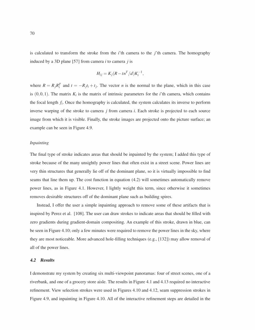
70

is calculated to transform the stroke from the i’th camera to the j’th camera. The homography

induced by a 3D plane [57] from camera i to camera j is

Hi j = Kj(R− tnT/d)K−1i ,

where R = R jRTi and t = −R jti + t j. The vector n is the normal to the plane, which in this case

is (0,0,1). The matrix Ki is the matrix of intrinsic parameters for the i’th camera, which contains

the focal length fi. Once the homography is calculated, the system calculates its inverse to perform

inverse warping of the stroke to camera j from camera i. Each stroke is projected to each source

image from which it is visible. Finally, the stroke images are projected onto the picture surface; an

example can be seen in Figure 4.9.

Inpainting

The final type of stroke indicates areas that should be inpainted by the system; I added this type of

stroke because of the many unsightly power lines that often exist in a street scene. Power lines are

very thin structures that generally lie off of the dominant plane, so it is virtually impossible to find

seams that line them up. The cost function in equation (4.2) will sometimes automatically remove

power lines, as in Figure 4.1. However, I lightly weight this term, since otherwise it sometimes

removes desirable structures off of the dominant plane such as building spires.

Instead, I offer the user a simple inpainting approach to remove some of these artifacts that is

inspired by Perez et al. [108]. The user can draw strokes to indicate areas that should be filled with

zero gradients during gradient-domain compositing. An example of this stroke, drawn in blue, can

be seen in Figure 4.10; only a few minutes were required to remove the power lines in the sky, where

they are most noticeable. More advanced hole-filling techniques (e.g., [132]) may allow removal of

all of the power lines.

4.2 Results

I demonstrate my system by creating six multi-viewpoint panoramas: four of street scenes, one of a

riverbank, and one of a grocery store aisle. The results in Figure 4.1 and 4.13 required no interactive

refinement. View selection strokes were used in Figures 4.10 and 4.12, seam suppression strokes in

Figure 4.9, and inpainting in Figure 4.10. All of the interactive refinement steps are detailed in the

71

Figure 4.9: A multi-viewpoint panorama of a street in Antwerp composed from 114 photographs. First row:the initial panorama computed automatically. The result is good except that several vehicles (highlightedin yellow) have been shortened. Second row: to fix the problem, the user draws one stroke on each car insome source photograph; shown here are strokes on the first, fifth, and eighth sources. Far right: the strokesare automatically propagated to all of the projected sources, of which the third is shown here. Ten strokeswere drawn in all, one for each vehicle. Third row: seams for final result. Fourth row: the final result afterinteractive refinement.

72

respective captions, and all of the input source photographs can be viewed on the project website.4

The effort by the user to produce the panoramas was fairly modest; for all of my results, the user

interaction time was less than the time required to capture the input photographs. The largest result

(Figure 4.10) took roughly 45 minutes to capture, and less than 20 minutes of interaction (ignoring

off-line computation).

The MRF optimization is not always able to produce good results automatically. The first row

of Figure 4.9 shows shortened cars caused by poor seams placed in areas in front of the dominant

plane. The middle of the scene in Figure 4.10 contains a large region off of the dominant plane; the

automatically stitched result in the first row is thus unnatural. Both of these errors were fixed by

interactive refinement. While careful examination of the final results will reveal occasional artifacts,

I feel that my images successfully visualize the scenes they depict. Notice that my scenes contain

significant geometry off of the dominant plane, such as crossing streets, trees, bushes, cars, etc., that

are depicted in their correct aspect ratios (which strip panoramas would squash or stretch). Also

notice that my panoramas are composed of large regions of ordinary perspective, rather than thin

strips.

My system is not able to produce effective multi-viewpoint panoramas for every scene. For ex-

ample, the streets that I demonstrate here are fairly urban; suburban scenes are more challenging

because the houses frequently lie at a range of different depths. My system works best when the

visible scene geometry frequently intersects the dominant plane, and the quality of the result de-

grades gracefully as the frequency of these intersections decreases. Some examples of failure cases

are included on the project website.

4.3 Future work

There are several ways I can improve my results. A simple approach I am beginning to explore

would handle shifts in the depth of the dominant plane. I have already shown that geometry at the

dominant plane is aligned between the projected source images. If the picture surface is parallel to

the camera path, however, a horizontal translation of the projected source images along the picture

surface can be used to align geometry at any plane parallel to the dominant plane (this observation

4http://grail.cs.washington.edu/projects/multipano/, which also includes full-resolution versions of allmy panoramas.

73

is true for the same reasons that a horizontal disparity can explain variations in depth for a stereo

pair of images). Such translations could be used to stabilize geometry in a scene where the dominant

plane shifts.

Another type of seam transition between viewpoints that my system does not currently exploit

is the depth discontinuity. When we see around the silhouette of an occluding object, we expect to

see geometry at some greater depth behind it. However, we are unlikely to notice if that geome-

try is depicted from a viewpoint slightly different from my own. I have experimentally confirmed

that such transitions appear natural; taking advantage of them automatically, however, requires ac-

curate recovery of scene depth and depth discontinuities. My experiments with multi-view stereo

techniques [67] suggest that this recovery is challenging for street scenes, since they contain many

windows and other reflective surfaces.

Finally, although I currently only demonstrate panoramas of “long” scenes, my approach should

also work for “long and tall” scenes. That is, one can imagine capturing a set of photographs along

a 2D grid, rather than a line, and compositing them into one image. Such an approach could be used

to image multiple floors of a mall or building atrium, which would be difficult to achieve with a

video sequence and strip panorama. I hope to capture and experiment with such a data set in the

near future.

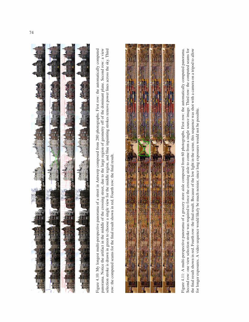
74

Fig

ure

4.10

:My

long

est

mul

ti-p

ersp

ectiv

epa

nora

ma

ofa

stre

etin

Ant

wer

pco

mpo

sed

from

280

phot

ogra

phs.

Firs

tro

w:

the

auto

mat

ical

lyco

mpu

ted

pano

ram

a.N

otic

eth

ear

tifac

tin

the

mid

dle

ofth

ecr

ossi

ngst

reet

,due

toth

ela

rge

regi

onof

geom

etry

off

ofth

edo

min

antp

lane

.Sec

ond

row

:avi

ewse

lect

ion

stro

keis

draw

nin

gree

nto

choo

sea

sing

levi

ewfo

rth

em

iddl

ere

gion

,and

blue

inpa

intin

gst

roke

sre

mov

epo

wer

lines

acro

ssth

esk

y.T

hird

row

:the

com

pute

dse

ams

for

the

final

resu

ltsh

own

inre

d.Fo

urth

row

:the

final

resu

lt.

Fig

ure

4.11

:Am

ulti

-per

spec

tive

pano

ram

aof

agr

ocer

yst

ore

aisl

eco

mpo

sed

from

60ph

otog

raph

s.Fi

rst

row

:the

auto

mat

ical

lyco

mpu

ted

pano

ram

a.Se

cond

row

:one

view

sele

ctio

nst

roke

was

requ

ired

tofo

rce

the

cros

sing

aisl

eto

com

efr

oma

sing

leso

urce

imag

e.T

hird

row

:the

com

pute

dse

ams

for

the

final

resu

ltsh

own

inre

d.Fo

urth

row

:the

final

resu

lt.B

ecau

seof

the

low

ligh

tin

the

scen

e,th

isse

quen

cew

assh

otw

ith

aca

mer

aon

atr

ipod

toal

low

for

long

erex

posu

res.

Avi

deo

sequ

ence

wou

ldlik

ely

bem

uch

nois

ier,

sinc

elo

ngex

posu

res

wou

ldno

tbe

poss

ible

.

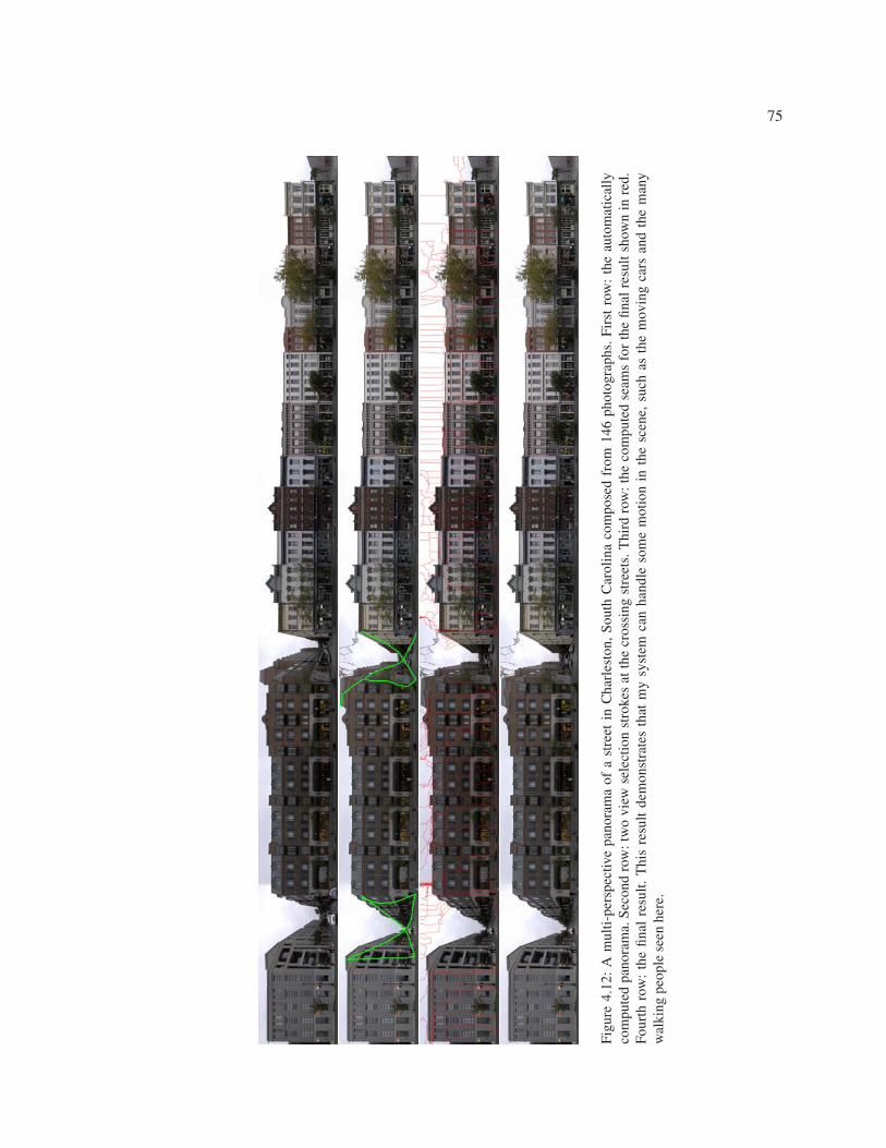
75

Fig

ure

4.12

:A

mul

ti-p

ersp

ectiv

epa

nora

ma

ofa

stre

etin

Cha

rles

ton,

Sout

hC

arol

ina

com

pose

dfr

om14

6ph

otog

raph

s.Fi

rst

row

:th

eau

tom

atic

ally

com

pute

dpa

nora

ma.

Sec

ond

row

:tw

ovi

ewse

lect

ion

stro

kes

atth

ecr

ossi

ngst

reet

s.T

hird

row

:the

com

pute

dse

ams

for

the

final

resu

ltsh

own

inre

d.Fo

urth

row

:th

efin

alre

sult.

Thi

sre

sult

dem

onst

rate

sth

atm

ysy

stem

can

hand

leso

me

mot

ion

inth

esc

ene,

such

asth

em

ovin

gca

rsan

dth

em

any

wal

king

peop

lese

enhe

re.

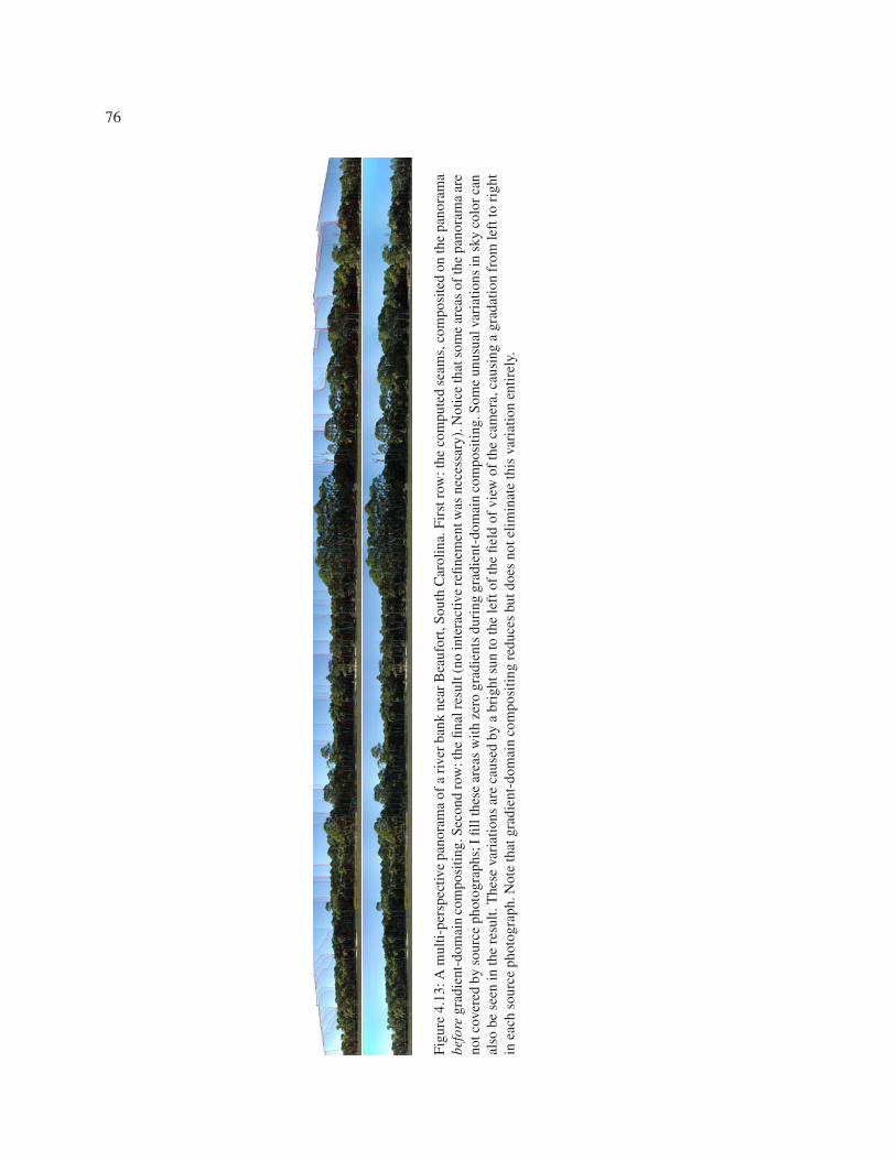
76

Figu

re4.

13:A

mul

ti-pe

rspe

ctiv

epa

nora

ma

ofa

rive

rba

nkne

arB

eauf

ort,

Sout

hC

arol

ina.

Firs

trow

:the

com

pute

dse

ams,

com

posi

ted

onth

epa

nora

ma

befo

regr

adie

nt-d

omai

nco

mpo

sitin

g.Se

cond

row

:the

final

resu

lt(n

oin

tera

ctiv

ere

finem

entw

asne

cess

ary)

.Not

ice

that

som

ear

eas

ofth

epa

nora

ma

are

notc

over

edby

sour

ceph

otog

raph

s;I

fill

thes

ear

eas

wit

hze

rogr

adie

nts

duri

nggr

adie

nt-d

omai

nco

mpo

siti

ng.S

ome

unus

ualv

aria

tion

sin

sky

colo

rcan

also

bese

enin

the

resu

lt.T

hese

vari

atio

nsar

eca

used

bya

brig

htsu

nto

the

left

ofth

efie

ldof

view

ofth

eca

mer

a,ca

usin

ga

grad

atio

nfr

omle

ftto

righ

tin

each

sour

ceph

otog

raph

.Not

eth

atgr

adie

nt-d

omai

nco

mpo

siti

ngre

duce

sbu

tdoe

sno

teli

min

ate

this

vari

atio

nen

tire

ly.

77

Chapter 5

PANORAMIC VIDEO TEXTURES

5.1 Introduction

In the previous two chapters I showed how fragments of photographs can be re-combined seamlessly

into a new depiction more effective than any of the originals. In this chapter1 I apply this approach

to video, with the goal of creating a more immersive depiction of a scene. In chapter 3 I used

the photomontage framework to create better image panoramas, in which a series of photos are

captured from a single viewpoint and stitched into a single large image. When viewed interactively

on a computer with software such as QuickTime VR [27], image panoramas offer a much more

immersive experience than simple snapshots with narrower fields of view. Indeed, panoramas are

now used quite commonly on the Web to provide virtual tours of hotels, museums, exotic travel

destinations, and the like.

When a scene is dynamic, however, an image panorama depicts a frozen moment of time that

can appear odd and fail to provide an immersive, visceral sense of “being there.” There are previous

efforts to create more dynamic panoramas; these include various hybrid image/video approaches

which play video elements inside of an image panorama [40, 63], as well as full video panora-

mas [99, 71, 140]. However, such video panoramas today have two major drawbacks:

1. They require some form of specialized hardware to create, e.g., multiple synchronized video

cameras [110], or a video camera looking through a fisheye lens or pointing at a panoramically

reflective mirror [96], which restricts the resolution of the acquired scene.2

2. They have a finite duration in time, with a specific beginning, middle, and end; this finite

duration can destroy the sense of immersion.

1The work described in this chapter was originally presented as a paper [5] at SIGGRAPH 2005.

2The output of such a lens or mirror system is limited to the resolution of a single video camera (640×480 NTSC or1280×720 HD), which is insufficient to create a panoramic, immersive experience that allows panning and zooming.By contrast, my panoramic video textures can reach 9 megapixels or more in size.

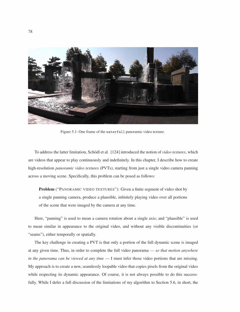
78

Figure 5.1: One frame of the waterfall panoramic video texture.

To address the latter limitation, Schodl et al. [124] introduced the notion of video textures, which

are videos that appear to play continuously and indefinitely. In this chapter, I describe how to create

high-resolution panoramic video textures (PVTs), starting from just a single video camera panning

across a moving scene. Specifically, this problem can be posed as follows:

Problem (“PANORAMIC VIDEO TEXTURES”): Given a finite segment of video shot by

a single panning camera, produce a plausible, infinitely playing video over all portions

of the scene that were imaged by the camera at any time.

Here, “panning” is used to mean a camera rotation about a single axis; and “plausible” is used

to mean similar in appearance to the original video, and without any visible discontinuities (or

“seams”), either temporally or spatially.

The key challenge in creating a PVT is that only a portion of the full dynamic scene is imaged

at any given time. Thus, in order to complete the full video panorama — so that motion anywhere

in the panorama can be viewed at any time — I must infer those video portions that are missing.

My approach is to create a new, seamlessly loopable video that copies pixels from the original video

while respecting its dynamic appearance. Of course, it is not always possible to do this success-

fully. While I defer a full discussion of the limitations of my algorithm to Section 5.6, in short, the

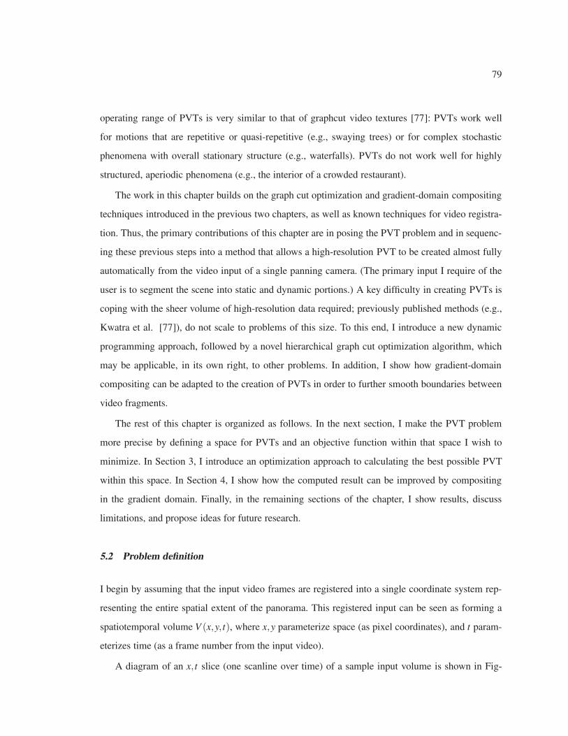
79

operating range of PVTs is very similar to that of graphcut video textures [77]: PVTs work well

for motions that are repetitive or quasi-repetitive (e.g., swaying trees) or for complex stochastic

phenomena with overall stationary structure (e.g., waterfalls). PVTs do not work well for highly

structured, aperiodic phenomena (e.g., the interior of a crowded restaurant).

The work in this chapter builds on the graph cut optimization and gradient-domain compositing

techniques introduced in the previous two chapters, as well as known techniques for video registra-

tion. Thus, the primary contributions of this chapter are in posing the PVT problem and in sequenc-

ing these previous steps into a method that allows a high-resolution PVT to be created almost fully

automatically from the video input of a single panning camera. (The primary input I require of the

user is to segment the scene into static and dynamic portions.) A key difficulty in creating PVTs is

coping with the sheer volume of high-resolution data required; previously published methods (e.g.,

Kwatra et al. [77]), do not scale to problems of this size. To this end, I introduce a new dynamic

programming approach, followed by a novel hierarchical graph cut optimization algorithm, which

may be applicable, in its own right, to other problems. In addition, I show how gradient-domain

compositing can be adapted to the creation of PVTs in order to further smooth boundaries between

video fragments.

The rest of this chapter is organized as follows. In the next section, I make the PVT problem

more precise by defining a space for PVTs and an objective function within that space I wish to

minimize. In Section 3, I introduce an optimization approach to calculating the best possible PVT

within this space. In Section 4, I show how the computed result can be improved by compositing

in the gradient domain. Finally, in the remaining sections of the chapter, I show results, discuss

limitations, and propose ideas for future research.

5.2 Problem definition

I begin by assuming that the input video frames are registered into a single coordinate system rep-

resenting the entire spatial extent of the panorama. This registered input can be seen as forming a

spatiotemporal volume V (x,y, t), where x,y parameterize space (as pixel coordinates), and t param-

eterizes time (as a frame number from the input video).

A diagram of an x, t slice (one scanline over time) of a sample input volume is shown in Fig-

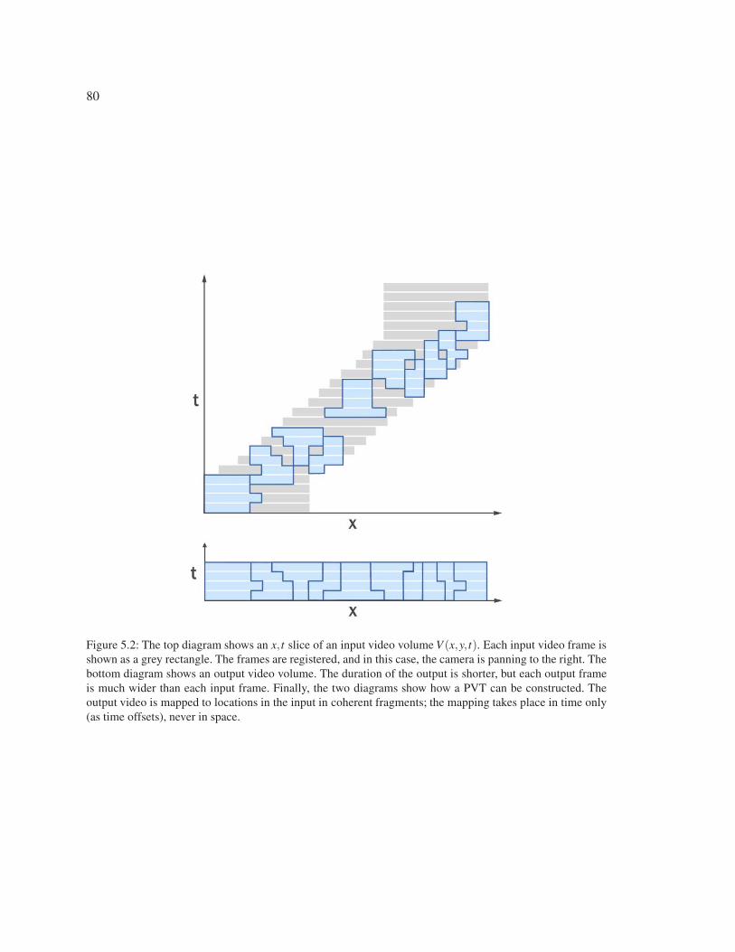
80

Figure 5.2: The top diagram shows an x,t slice of an input video volume V (x,y, t). Each input video frame isshown as a grey rectangle. The frames are registered, and in this case, the camera is panning to the right. Thebottom diagram shows an output video volume. The duration of the output is shorter, but each output frameis much wider than each input frame. Finally, the two diagrams show how a PVT can be constructed. Theoutput video is mapped to locations in the input in coherent fragments; the mapping takes place in time only(as time offsets), never in space.

81

Figure 5.3: A simple approach to creating a PVT would be to map a continuous diagonal slice of the inputvideo volume to the output panorama, regardless of appearance. This approach creates a valid result, butunnecessarily shears spatial structures across time (see Figure 5.4).

ure 5.2. Each input video frame provides color for only a small portion of this 3D space (the grey

rectangles in Figure 5.2); I use the notation V (x,y, t) = /0 to indicate that (x,y) falls outside the

bounding box of the input video frame at time t, and thus has no valid color.

My approach to constructing a PVT is to copy pixels from the input video to the output. There-

fore, a PVT is represented as a mapping Δ from any pixel in the output panoramic video texture to a

pixel in the input. I simplify the problem by assuming that pixels can be mapped in time but never in

space. Thus, for any output pixel p = (x,y, t), the mapping Δ(p) is a vector of the form (0,0,δ (p)),

which maps (x,y, t) to (x, y, t + δ (x,y, t)). Notice that each pixel in the same piece of copied video

in Figure 5.2 will have the same time-offset value δ .

The space of all possible PVTs is clearly quite large. One simple approach to creating a PVT

might be to choose time offsets that take a sheared rectangular slice through the input volume and

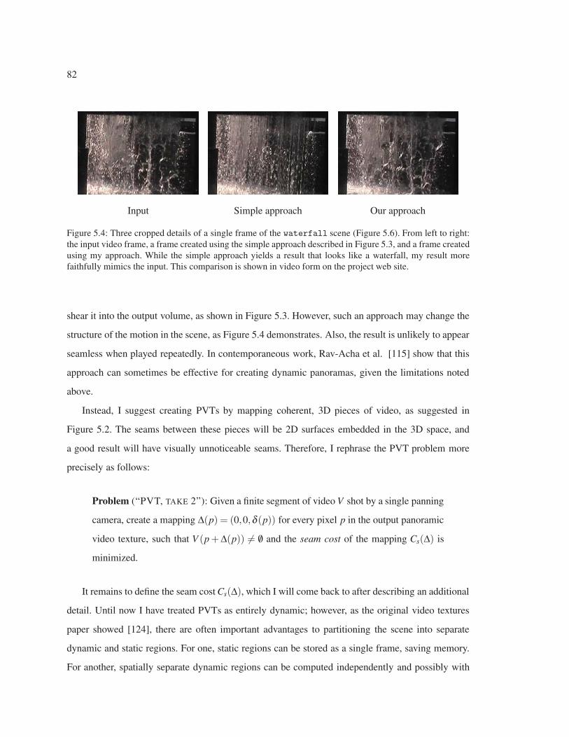
82

Input Simple approach Our approach

Figure 5.4: Three cropped details of a single frame of the waterfall scene (Figure 5.6). From left to right:the input video frame, a frame created using the simple approach described in Figure 5.3, and a frame createdusing my approach. While the simple approach yields a result that looks like a waterfall, my result morefaithfully mimics the input. This comparison is shown in video form on the project web site.

shear it into the output volume, as shown in Figure 5.3. However, such an approach may change the

structure of the motion in the scene, as Figure 5.4 demonstrates. Also, the result is unlikely to appear

seamless when played repeatedly. In contemporaneous work, Rav-Acha et al. [115] show that this

approach can sometimes be effective for creating dynamic panoramas, given the limitations noted

above.

Instead, I suggest creating PVTs by mapping coherent, 3D pieces of video, as suggested in

Figure 5.2. The seams between these pieces will be 2D surfaces embedded in the 3D space, and

a good result will have visually unnoticeable seams. Therefore, I rephrase the PVT problem more

precisely as follows:

Problem (“PVT, TAKE 2”): Given a finite segment of video V shot by a single panning

camera, create a mapping Δ(p) = (0,0,δ (p)) for every pixel p in the output panoramic

video texture, such that V (p + Δ(p)) �= /0 and the seam cost of the mapping Cs(Δ) is

minimized.

It remains to define the seam cost Cs(Δ), which I will come back to after describing an additional

detail. Until now I have treated PVTs as entirely dynamic; however, as the original video textures

paper showed [124], there are often important advantages to partitioning the scene into separate

dynamic and static regions. For one, static regions can be stored as a single frame, saving memory.

For another, spatially separate dynamic regions can be computed independently and possibly with

83

different durations, which is useful if they portray phenomena with different periodicities.

For these reasons, I define a single static background layer B(x,y). This background layer con-

tains a color for each pixel in the user-specified static regions, while B(x,y) = /0 for those pixels in

the dynamic regions. I also define a binary matte D for the dynamic regions of the output panoramic

video texture. I set D to the dilation of the null-valued regions of B(x,y); thus, D overlaps the non-

null regions of B along a one-pixel-wide boundary. I can use this overlap to ensure a seamless match

between the dynamic and static portions of the output PVT. For convenience, I also treat D as a

domain, so that (x,y) ∈ D implies that (x,y) is in the dynamic portion of the binary matte.

With these definitions, I can define the seam cost:

Cs(Δ) = ∑p=(x,y,t) |(x,y)∈D

(Cb(Δ, p) + Cv(Δ, p)) (5.1)

where

Cb(Δ, p) =

⎧⎪⎨⎪⎩

‖V (p+ Δ(p))−B(p)‖k if B(p) �= /0;

0 otherwise.

and

Cv(Δ, p) =3

∑i=1

⎧⎪⎨⎪⎩

‖V (p+ Δ(p))−V (p+ Δ(p+ ei))‖k if p + ei ∈ D;

0 otherwise.

Here, e1, e2, and e3 are the unit vectors (1,0,0), (0,1,0), and (0,0,1), respectively; and k is a

constant, used as an exponent on the L2 norm: I use k = 8. The definition of the seam cost assumes

that the constraint V (p+ Δ(p)) �= /0 for each p ∈ D is satisfied.

Thus, the seam cost sums two terms over all pixels p in the dynamic portion of the output PVT.

The first term is the difference between the pixel values in the dynamic scene and the static scene if

p is on the boundary where the two overlap. The second term is the difference between the value of

the pixel that p maps to in the original video and the value of the pixel that p would map to if it had

the same time offset as its neighbor, for neighbors in all three cardinal directions. (In all cases, the

difference is raised to the k-th power to penalize instances of higher color difference across a seam.)

One final note: in order to ensure that the PVT loops seamlessly, I define

Δ(x,y, t) = Δ(x, y, t mod tmax)

for all t, where tmax is the duration of the PVT. I discuss how tmax is determined, as well as the

mapping Δ itself, in the next section.

84

5.3 Our approach

Notice that the cost function Cs maps onto a 3D Markov Random Field (MRF), where D× [0..tmax]

is the domain and Δ(p) (or, equivalently, δ (p)) are the free variables for which I need to solve. As in

the previous two chapters, I can thus use MRF optimization to minimize it. Algorithms for solving

this type of problem include belief propagation [42] and graph cuts [74].

Unfortunately, the scale of the problem is intractably large. A typical aligned input video is

6000× 1200 pixels spatially, and thousands of frames long. In my experiments, the typical output

video is 35 frames long, and any one pixel p has about 500 choices for δ (p). Thus, the typical

output volume has 2.5×108 variables, each with 500 possible values. A straightforward application

of standard MRF algorithms would require more memory and compute power than is currently

available. I therefore designed an accelerated algorithm to compute a result.

Note that if a dynamic region is small enough to fit entirely within the bounding box of a range of

tmax input frames, its video texture can be created using existing techniques [77]. For larger regions

that do not meet that constraint, however, I use the following approach to integrate portions of the

input video over space and time.

I first register the video frames, and then separate the PVT into static and dynamic regions.

These are the only steps that require any manual user input. I then compute, for each dynamic

region, a good loop length for that portion of the PVT. Finally, I solve for the mapping Δ. The first

step of the solution is to minimize a heavily constrained version of the optimization problem using

dynamic programming at a sub-sampled resolution. I then loosen the constraints and use graph cut

optimization to refine the solution. The final step uses hierarchical graph cut optimization to refine

this sub-sampled solution at the full resolution.

5.3.1 Video registration

Video registration is a well-studied problem, and continues to be an active area of research. I simply

use existing techniques for registration (my own contributions begin after this preprocessing step).

Specifically, I use a feature-based alignment method [22], followed by a global bundle adjustment

step [137] to align all the video frames simultaneously with each other. I use a three-parameter 3D

rotation motion model [134]. Once the motion parameters are recovered, I warp the video frames

85

into a single coordinate system by projecting them onto a cylindrical surface.

The video registration step, using existing techniques, is not always entirely successful. In order

to improve the registration results, it is sometimes helpful to allow a user to manually mask out

moving parts of the input video, due either to actual object motion or to scene parallax, so that they

are not incorrectly used in the registration process. The masking required for the scenes I have tried

is discussed in more detail in Section 5.5.

5.3.2 Static and dynamic regions

Schodl et al. [124] showed that the dynamic regions of a scene could be identified by thresholding

the variance of each pixel across time. However, I found that errors and jitter in my registration step,

as well as MPEG compression noise from my digital camera, made the variance of static regions as

high or higher than the variance of gently moving areas, such as rippling water. I thus ask the user

to draw a single mask for each sequence. Apart from any manual masking that might be required to

improve the video registration, this is the only manual part of my PVT generation process.

Given a user-drawn mask, I create a single panorama for the static regions; I first dilate the mask

once to create an overlap between static and dynamic regions, and then create the static panorama

automatically using the panoramic stitching approach described in chapter 3.

5.3.3 Looping length

In each dynamic region, the duration tmax of the output video should match the natural periodicity

of that region. I thus automatically determine the natural period within a preset range �min . . . �max by

examining the input video within the dynamic region. I typically set �min = 30 and �max = 60, since

shorter lengths are too repetitive, and longer lengths require higher output bandwidth and compute

time. To determine the best loop length tmax, each input frame t is compared to each input frame in

the range (t + �min, t + �max) that spatially overlaps with frame t by at least 50%. The comparison

is a simple sum of squared differences in RGB values, normalized by the number of overlap pixels.

I find the pair of frames t, t + l that best minimizes this comparison, and set tmax(t) to �− 1. This

approach is very simple, but in the data sets I have tried it works well.

86

Figure 5.5: A possible solution to the constrained formulation described in Section 5.3.4, where a continuousspan of video pixels across y and t is copied to each column of the output. The solution shown here uses only6 different values of Δ(p).

5.3.4 A constrained formulation

The first step in creating a PVT for each dynamic region is to solve a heavily constrained version

of the overall problem. I motivate these constraints with an observation. If a seam between spatially

neighboring pixels is visually unnoticeable at a certain frame t, the seam between the same two

pixels tends to be unnoticeable in the frames before and after t. Although this observation is some-

times wrong, temporal coherence in the scene makes it correct more often than not. Thus, one way

to significantly reduce the search space is to assume that, at each output location (x,y), there is just

a single time offset δ , regardless of t. This constraint reduces the search space from a 3D MRF to a

2D MRF. However, the 2D MRF would still be expensive to compute, since a seam penalty between

neighboring output pixels would require comparing a span of pixels across time.

An additional constraint can be added to reduce the problem to a 1D Markov model. Since the

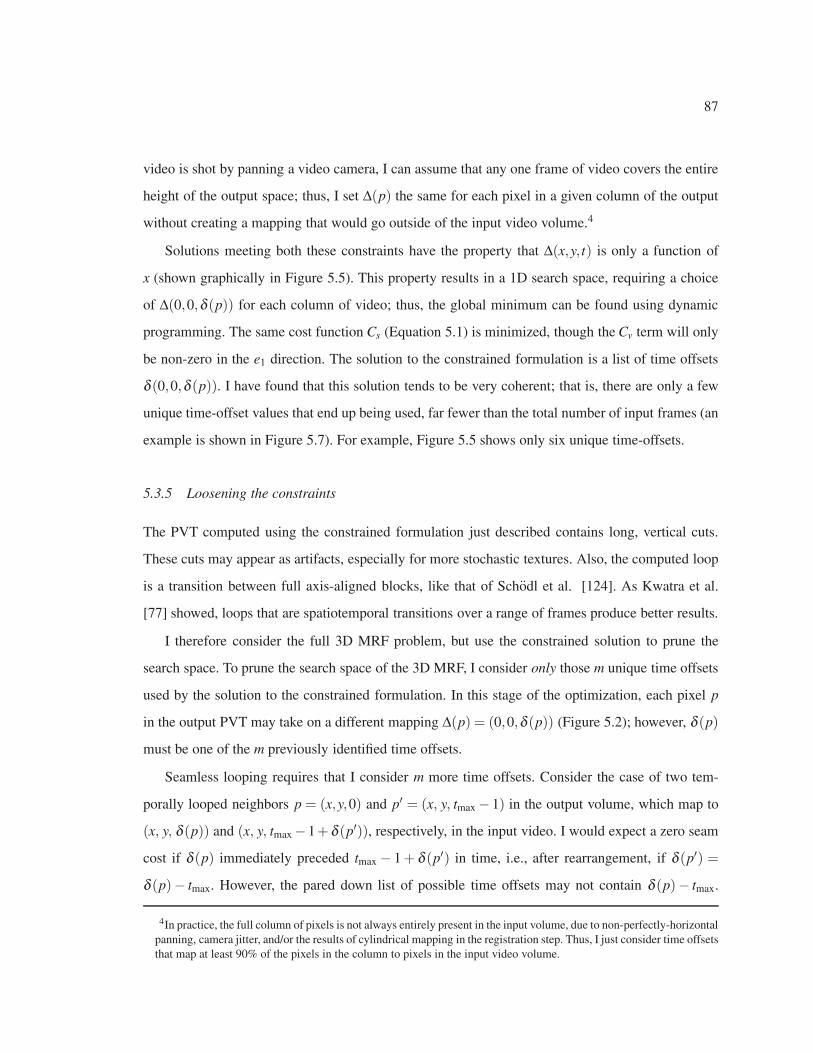
87

video is shot by panning a video camera, I can assume that any one frame of video covers the entire

height of the output space; thus, I set Δ(p) the same for each pixel in a given column of the output

without creating a mapping that would go outside of the input video volume.4

Solutions meeting both these constraints have the property that Δ(x,y, t) is only a function of

x (shown graphically in Figure 5.5). This property results in a 1D search space, requiring a choice

of Δ(0,0,δ (p)) for each column of video; thus, the global minimum can be found using dynamic

programming. The same cost function Cs (Equation 5.1) is minimized, though the Cv term will only

be non-zero in the e1 direction. The solution to the constrained formulation is a list of time offsets

δ (0,0,δ (p)). I have found that this solution tends to be very coherent; that is, there are only a few

unique time-offset values that end up being used, far fewer than the total number of input frames (an

example is shown in Figure 5.7). For example, Figure 5.5 shows only six unique time-offsets.

5.3.5 Loosening the constraints

The PVT computed using the constrained formulation just described contains long, vertical cuts.

These cuts may appear as artifacts, especially for more stochastic textures. Also, the computed loop

is a transition between full axis-aligned blocks, like that of Schodl et al. [124]. As Kwatra et al.

[77] showed, loops that are spatiotemporal transitions over a range of frames produce better results.

I therefore consider the full 3D MRF problem, but use the constrained solution to prune the

search space. To prune the search space of the 3D MRF, I consider only those m unique time offsets

used by the solution to the constrained formulation. In this stage of the optimization, each pixel p

in the output PVT may take on a different mapping Δ(p) = (0,0,δ (p)) (Figure 5.2); however, δ (p)

must be one of the m previously identified time offsets.

Seamless looping requires that I consider m more time offsets. Consider the case of two tem-

porally looped neighbors p = (x,y,0) and p′ = (x, y, tmax − 1) in the output volume, which map to

(x, y, δ (p)) and (x, y, tmax −1+ δ (p′)), respectively, in the input video. I would expect a zero seam

cost if δ (p) immediately preceded tmax − 1 + δ (p′) in time, i.e., after rearrangement, if δ (p′) =

δ (p)− tmax. However, the pared down list of possible time offsets may not contain δ (p)− tmax.

4In practice, the full column of pixels is not always entirely present in the input volume, due to non-perfectly-horizontalpanning, camera jitter, and/or the results of cylindrical mapping in the registration step. Thus, I just consider time offsetsthat map at least 90% of the pixels in the column to pixels in the input video volume.

88

Thus, to allow for a zero-cost transition in this case, I augment the set of labels to include m addi-

tional labels, δ (x,0,0)− tmax.

Given this reduced search space, iterative graph cut optimization is used to solve the more gen-

eral 3D MRF. This optimization is executed in a series of alpha expansion moves [74]. Each ex-

pansion chooses a single time-offset α and expands it. During an expansion move, each pixel p

can maintain its current time-offset δ (p), or switch to α . To reach a near-global minimum of the

objective function, I can iterate over each possible value of α and expand it, and continue to do so

until consecutively expanding each α fails to further reduce the total cost.

To perform an alpha expansion, I define a three-dimensional graph with each node representing

one pixel in the output video volume, and solve for the minimum cut. Details on the graph setup can

be found in Kolmogorov and Zabih [74]. In their terminology, during a single alpha expansion the

Cb(Δ, p) term of the seam cost is a function of a single binary variable, and Cv(Δ, p) is a function of

two (neighboring) binary variables.

It is advantageous to minimize the size of the graph, since memory consumption and processing

time scale with it. In general, it is not necessary to create a node for each pixel in the video volume.

For example, Kolmogorov and Zabih do not create nodes for pixels already assigned time offset α ,

since their time offset will not change during alpha expansion. I also prune nodes in this fashion;

however, my application offers another opportunity for pruning. In particular, for a given α , I do

not create nodes corresponding to output pixels p for which V (p + (0,0,α)) = /0. This pruning

enforces the constraint V (p+Δ(p)) �= /0 given in the PVT problem definition, and it also significantly

improves efficiency. The spatial resolution of the graph becomes limited by the dimensions of an

input video frame, rather than the dimensions of the entire panorama.

While pruning improves the efficiency of the optimization, I still found that performing a graph

cut at full resolution can overwhelm the memory and processing capabilities of current computers.

I thus present a novel, hierarchical MRF optimization approach that allows us to compute the final

result.

89

5.3.6 Hierarchical graph cut optimization

A common approach for building hierarchical algorithms in computer vision [16] is to first compute

a solution at a coarser resolution. This result is then used to initialize the computation at the finer

resolution, helping to avoid local minima. This approach is not immediately applicable; I cannot

compute a solution at the finer resolution because the memory requirements are too high. Instead,

I use the computed solution at a coarser spatial resolution to prune the graph when computing at

the finer resolution. My intuition is that the computed seams at the finer resolution will be roughly

similar to the ones at the coarse resolution, but that the additional image information will cause local

changes. I thus only optimize within the neighborhood of the seams found at the coarse resolution.

Specifically, given a result δ (k)(x,y, t) computed at a coarser spatial resolution, I first create the

finer resolution solution δ (k+1)(x,y, t) by up-sampling δ (k)(x,y, t). Then, when expanding α , I first

add to the graph only those video pixels not assigned α that neighbor an α-assigned pixel. That is,

I add pixels along the boundary between α and non-α . Finally, I dilate this boundary set of nodes

s times (typically 10) and add these new nodes to the graph (while respecting pruning rules already

mentioned). I then compute the expansion on this limited graph.

Note that this hierarchical approach is more susceptible to local minima than standard alpha-

expansion. The minimum found by the alpha-expansion algorithm is provably close to the global

minimum (when the energy function meets certain requirements [74]); my pruning technique loses

this guarantee. However, in practice, in which I typically use 2 or 3 levels in the hierarchy, I have

found the technique to work well.

5.4 Gradient-domain compositing

The result computed using optimization can still exhibit visual artifacts for several reasons. Al-

though I lock exposure on the video camera, I still found some exposure variations in the recorded

images. Also, it is sometimes impossible to find seams that are completely natural (some reasons

are discussed in Section 5.6). Finally, small errors in the alignment procedure can also create visual

artifacts. To improve results I composite the video fragments in the gradient domain, by treating the

video as sources of color gradients rather than color magnitudes.

This basic approach is not new. Perez et al. [108] first demonstrated the efficacy of gradient-

90

domain techniques for combining 2D images. In chapter 3 I showed that gradient-domain composit-

ing, in combination with MRF optimization, can yield better results than either technique alone.

However, simply applying this 2D approach separately to each frame of a composited video can

lead to poor temporal coherence in the form of color flashing. To address this, Wang et al. [142]

extended these 2D approaches to spatiotemporal 3D in order to combine videos in the gradient

domain. I build on the work of Wang et al. to solve my problem.

I first create a 2D gradient field for the still regions of the scene. This gradient field is then

integrated to form the still panorama. Next, a 3D gradient field is formed for the dynamic regions of

the scene, and integrated to create video textures. Integrating the gradient field requires the solution

of a large, linear system of equations. A full derivation of this system can be found in Wang et al.

; I describe only the unique aspects of my system. For one, I wish to ensure that seams between

still and dynamic regions are minimized; this requires a judicious choice of boundary conditions.

Secondly, I want to make sure the video loops seamlessly.

5.4.1 Boundary conditions

Any application of gradient-domain techniques first requires a choice of boundary conditions, which

describe how to handle gradients at the boundaries of the domain. Dirichlet boundary conditions,

like those used by Perez et al. , are suitable if the colors of the boundary pixels outside the domain

are known. If they are not known, as in the photomontage system of chapter 3 and the work of

Wang et al. , the weaker Neumann boundary conditions must be used. The mathematical definition

of these boundary conditions can be found in the cited papers.

A mix of both of these boundary conditions is needed in my case. For boundary pixels of dy-

namic regions that are adjacent to pixels within the still background panorama, the colors of these

adjacent pixels are known; I can thus use Dirichlet boundary conditions. For boundary pixels that

lie along the boundary of the entire scene, the colors of adjacent pixels outside the domain are not

known; they are outside the region captured by the video camera. For these I use Neumann boundary

conditions.

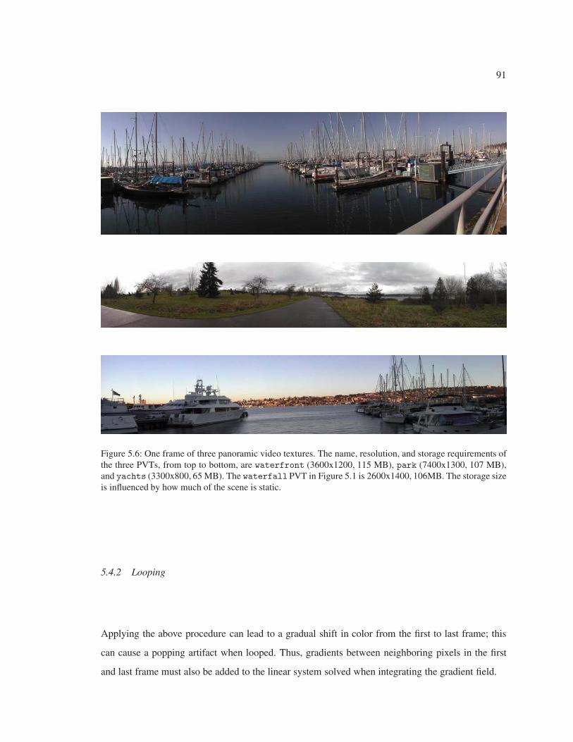
91

Figure 5.6: One frame of three panoramic video textures. The name, resolution, and storage requirements ofthe three PVTs, from top to bottom, are waterfront (3600x1200, 115 MB), park (7400x1300, 107 MB),and yachts (3300x800, 65 MB). The waterfall PVT in Figure 5.1 is 2600x1400, 106MB. The storage sizeis influenced by how much of the scene is static.

5.4.2 Looping

Applying the above procedure can lead to a gradual shift in color from the first to last frame; this

can cause a popping artifact when looped. Thus, gradients between neighboring pixels in the first

and last frame must also be added to the linear system solved when integrating the gradient field.

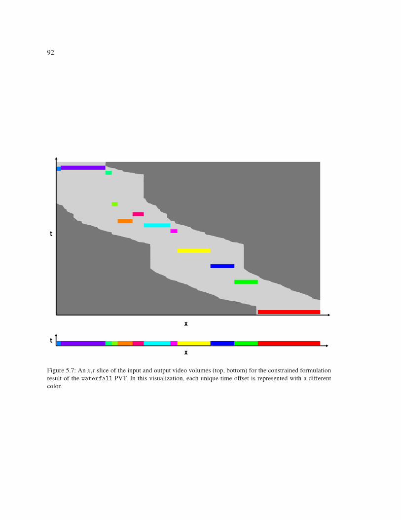
92

Figure 5.7: An x,t slice of the input and output video volumes (top, bottom) for the constrained formulationresult of the waterfall PVT. In this visualization, each unique time offset is represented with a differentcolor.

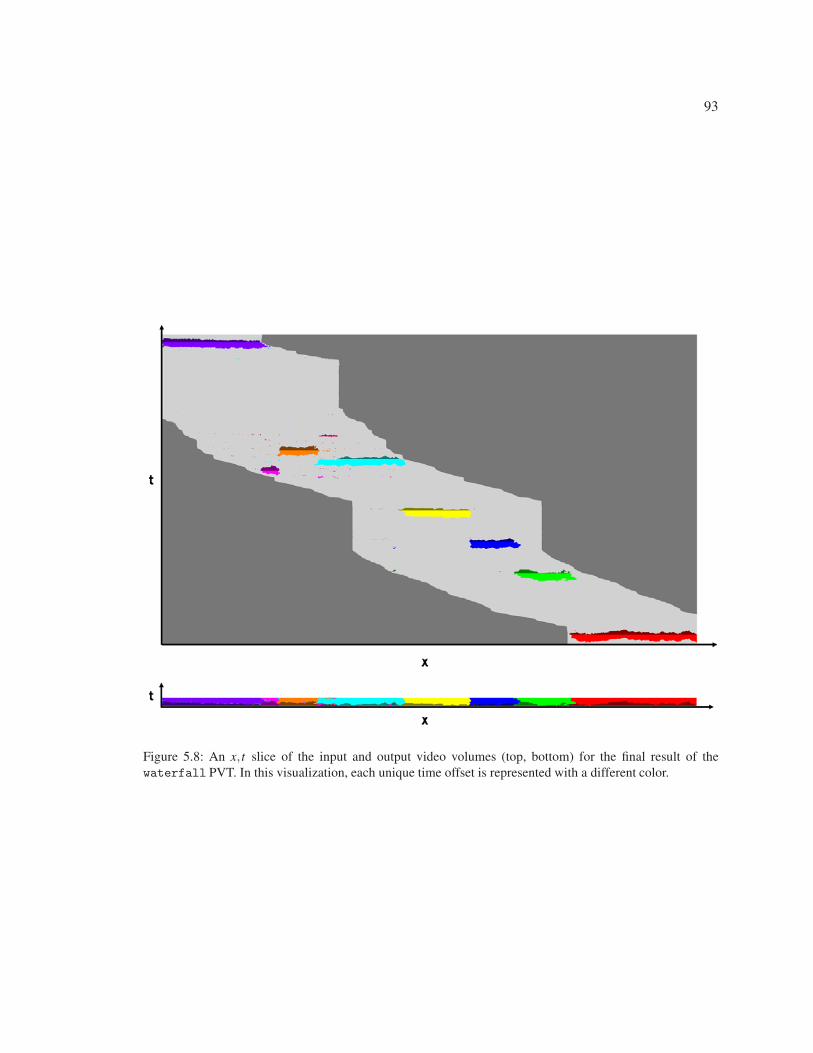
93

Figure 5.8: An x,t slice of the input and output video volumes (top, bottom) for the final result of thewaterfall PVT. In this visualization, each unique time offset is represented with a different color.

94

5.5 Results

I show four panoramic scenes as results. My results are best viewed within my interactive viewer,

which can be downloaded from my project web site3; however, one frame of each result is shown

in Figures 5.1 and 5.6. Three of these panoramas were shot with an HD video camera in portrait

mode, with a vertical resolution of 1280 pixels, and one was shot with a standard video camera,

with a vertical resolution of 720. I typically shot about two minutes of video for each scene, and

wwas careful to leave the camera still at the beginning and end to capture enough material near the

boundaries of the scene. (Full 360-degree PVTs should also be possible, and would not in principle

require dwelling at the beginning or end.) The exposure control on each camera was locked, but

auto-focus was enabled.

Figures 5.7 and 5.8 visualize an x, t slice of the output and input video volumes for the waterfall

result; the latter figure shows the result of the constrained formulation (Section 5.3.4), while the for-

mer figure shows the result after loosening the constraints (Section 5.3.5).

In general, the results are compelling and immersive, although careful examination does reveal

the occasional artifact. When looking for artifacts, it is important to see if the artifact also exists

in the input video. For example, there are blurry areas that arise from the limited depth of field

of the camera, and noise from MPEG compression. The most noticeable artifacts, in my opinion,

come from jitter and drift in the alignment. For example, jitter in a dynamic region becomes more

noticeable when it is adjacent to to a perfectly still, static region.

5.5.1 Performance and human effort

The main human effort required to create a panoramic video texture is the drawing of a single mask;

this mask does not need to be exact, and generally took us about ten minutes to create.

The automatic registration of video frames is not completely successful; the results contain

jitter and drift. Scenes that lead to attractive panoramic video textures tend to contain significant

motion, and this motion can be problematic for current alignment techniques. For example, the

bottom twenty percent of the waterfront scene is filled with motion that causes significant jitter;

so I cropped this region out before alignment. Techniques for registering non-rigid scenes [41] may

3http://grail.cs.washington.edu/projects/panovidtex/

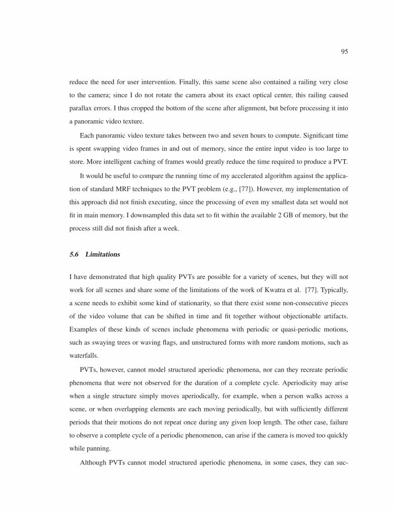
95

reduce the need for user intervention. Finally, this same scene also contained a railing very close

to the camera; since I do not rotate the camera about its exact optical center, this railing caused

parallax errors. I thus cropped the bottom of the scene after alignment, but before processing it into

a panoramic video texture.

Each panoramic video texture takes between two and seven hours to compute. Significant time

is spent swapping video frames in and out of memory, since the entire input video is too large to

store. More intelligent caching of frames would greatly reduce the time required to produce a PVT.

It would be useful to compare the running time of my accelerated algorithm against the applica-

tion of standard MRF techniques to the PVT problem (e.g., [77]). However, my implementation of

this approach did not finish executing, since the processing of even my smallest data set would not

fit in main memory. I downsampled this data set to fit within the available 2 GB of memory, but the

process still did not finish after a week.

5.6 Limitations

I have demonstrated that high quality PVTs are possible for a variety of scenes, but they will not

work for all scenes and share some of the limitations of the work of Kwatra et al. [77]. Typically,

a scene needs to exhibit some kind of stationarity, so that there exist some non-consecutive pieces

of the video volume that can be shifted in time and fit together without objectionable artifacts.

Examples of these kinds of scenes include phenomena with periodic or quasi-periodic motions,

such as swaying trees or waving flags, and unstructured forms with more random motions, such as

waterfalls.

PVTs, however, cannot model structured aperiodic phenomena, nor can they recreate periodic

phenomena that were not observed for the duration of a complete cycle. Aperiodicity may arise

when a single structure simply moves aperiodically, for example, when a person walks across a

scene, or when overlapping elements are each moving periodically, but with sufficiently different

periods that their motions do not repeat once during any given loop length. The other case, failure

to observe a complete cycle of a periodic phenomenon, can arise if the camera is moved too quickly

while panning.

Although PVTs cannot model structured aperiodic phenomena, in some cases, they can suc-

96

cessfully omit them altogether. For instance, if a person walks across a scene that otherwise meets

the criteria for a good PVT, the optimization algorithm will favor omitting the pixels correspond-

ing to that person and fill in with observations from other moments in time. The input video of the

waterfall scene, for example, contains flying birds and passing people; both are automatically

omitted in the final PVT. (Another approach to handling objects such as this is to include them as

“frozen” forms in the static portion of the panorama.)

My system will sometimes produce good results for scenes that do not strictly match my as-

sumptions. For example, the yachts scene contains cars on a highway in the distance. The algo-

rithm takes advantage of occluding trees and boat masts to produce a seamless result. The distant

cars seem to just disappear once they pass behind the occluders, but the overall effect is perceived

as quite natural.

5.7 Future work

There are many good areas for future work. The ability to handle scenes with various “foreground

characters” (a.k.a. “video sprites” [124]) would greatly increase the applicability of my system. I

could also eliminate the need for user interaction by automatically segmenting the scene into dy-

namic and still regions. This segmentation could also be used to improve the automatic registration

of the video frames. Audio would greatly enhance the immersiveness of my results; the audio would

require similar texturing techniques, and could follow movements within the interactive viewer. The

output of multiple capture devices could be combined into one panorama. For example, the static

regions could be captured with a still camera to allow greater resolution. Also, I currently require the

camera to pan across the scene; it would be straightforward to loosen this constraint to allow pan and

tilt, though the optimization problem would be less constrained, requiring more computation time.

Finally, I currently lock the exposure on the camera. Ideally, I would let the camera choose the best

exposure dynamically to create high-dynamic-range, panoramic video textures. This enhancement

would involve mapping the input frames to radiance space before applying my computations.

97

5.8 Conclusion

One of the great promises of computer graphics is to someday create a totally immersive experience,

engaging all five senses in a convincing environment that could be entirely synthetic. Panoramic

photography is an early technology that provides a limited form of immersion. Video textures en-

hance the illusion of presence, allowing dynamic phenomena to play continuously without any vi-

sual seams or obvious repetition. Panoramic video textures combine these two approaches to create

what might be considered a new medium that is greater than the sum of its parts: The experience of

roaming around at will in a continuous, panoramic, high-resolution, moving scene is qualitatively

quite different from either panning around in a static scene or watching a single video texture play.

In the not so distant future, I envision panoramic video textures being employed quite commonly

on the Web, just as image panoramas are today. There, they will provide a much more compelling

sense of “being there,” allowing people to learn about and enjoy distant places — and share their

own experiences — in captivating new ways.

98

Chapter 6

CONCLUSION

6.1 Contributions

In this thesis I have designed a novel approach to combining multiple samples of the plenoptic

function into new depictions, and applied this approach to several different depiction tasks. To apply

this approach I begin by identifying the goals of the new depiction, and then formulate those goals

in the form of a Markov Random Field cost function. This cost function is minimized via graph cuts

to produce a solution. Finally, the final depiction is created by compositing the result of the graph

cut optimization in the gradient domain.

I applied this approach in three chapters. In chapter 3, I introduced the overall approach as

well an interactive system that allows a user to design a photomontage by specifying high-level

objectives it should exhibit, either globally or locally through a painting interface. The input to this

system was typically a series of photographs from a single viewpoint; in chapter 4 I extended this

approach to sequences of photographs captured from shifted viewpoints, with the goal of creating

multi-viewpoint panoramas of long scenes. To accomplish good results I formulated the qualities

the panorama should exhibit in order to mimic the properties of multi-viewpoint panoramas created

by artist Michael Koller [73]. Finally, in chapter 5 I extended my approach to video sequences, in

order to create immersive depictions of a scene that were both panoramic and dynamic. Along with

this overall approach to combining multiple samples into more effective depictions, my thesis makes

several contributions.

• Combining graph cuts and gradient-domain techniques. I primarily uses two technical

components – computing seams for image composition using graph cuts [77], and composit-

ing image regions in the gradient-domain [108] – which were not invented here. However, in

this thesis I demonstrate that the combination of these two techniques is much more powerful

than either alone for combining images and video.

99

• A versatile framework. I demonstrate an overall framework for authoring depictions by spec-

ifying high-level goals; an algorithm then constructs the depiction by optimizing over multiple

samples. I demonstrate a wide range of applications for which this framework is useful.

• A user interaction metaphor. The photomontage system includes a novel user interface

which encourages a user to consider a stack of images as a single entity, pieces of which

contain the desired appearance.

• A practical approach to creating multi-viewpoint panoramas. The approach I demonstrate

is able to take as input a sparse collection of hand-held photographs (unlike previous work),

and is able to generate very high-quality and high-resolution results.

• A new medium: panoramic video textures. PVTs are a new medium somewhere between

panoramic photographs and video. Unlike a photograph the depiction is dynamic, and unlike

video the depiction does not have a finite duration.

• An efficient algorithm for computing high-resolution panoramic video textures. I use a

dynamic programming step as well as a novel hierarchical graph cut algorithm to compute

a result in reasonable time and memory requirements, which would not be possible using

existing algorithms.

6.2 Future work

The approach I describe may very well be useful for applications that are not foreseen in this thesis.

At the end of chapters 3-5, I discussed limitations and potential areas of future work to improve

on the techniques described. In the rest of thesis, however, I will suggest more ambitious ideas for

future research projects that combine information from multiple samples of the plenoptic function.

These ideas do not necessarily follow the approach described above.

6.2.1 Computer-assisted rephotography

Rephotography is the act of capturing a repeat photograph of a scene; that is, reproducing an earlier

photograph but with a time lag between the two images. Rephotographs provide a “then and now”

100

visualization of a scene and the changes that have occurred over time. They are also very challeng-

ing to produce, since the rephotograph must be captured from the exact same viewpoint and field

of view, and sometimes the same time of day and season. Rephotography is common in the study

of history (such as the “third view” rephotographic survey of famous landscape photographs of the

American west [72]), and for geological monitoring of erosion and other time-varying phenom-

ena [56].

The challenge of capturing a rephotograph can be situated within the framework described in

chapter 2, specifically within the alignment phase. The goal is to capture a new sample of the plenop-

tic function identical to an existing sample, where the only variation occurs over the time-axis of

the plenoptic function. This alignment task must, of course, occur during capture time; I thus pro-

pose creating a real-time, interactive system that helps a photographer to capture a rephotograph.

I envision attaching a video camera to the back of a tabletPC, thus approximating the form fac-

tor of existing digital cameras but with a larger screen and a more flexible computer. The system

would, in real-time, tell the user where to move to better align his/her viewpoint to the viewpoint

of the older photograph. To perform this task, the system could take advantage of SIFT [84] feature

matches between the old and new views, in order to establish their epipolar geometry [57]. An anal-

ysis of this epipolar geometry should reveal the translation direction necessary to align the views.

Correct camera rotation can be achieved after capture by warping the new view with an appropriate

homography.

In general, this project points to an interesting direction – performing more computation during

capture time in order to aid a user in capturing a desired sample of the plenoptic function. As

computers on cameras become more powerful, we should be able develop computational approaches

that improve our ability to capture good photographs and videos.

6.2.2 Motion parallax textures

Digital photographs can depict a scene in high resolution, but they often fail to communicate the

depth of objects in a scene. Humans, for the most part, perceive depth using two eyes. Even with

only one eye open, however, humans are able to perceive depth by slightly moving our heads; this

motion shifts the viewpoint and induces motion parallax. Motion parallax, which describes how

101

objects further away move less than closer objects when the viewpoint is shifted, is an important

cue for perceiving depth.

Imbuing photographs with motion parallax would allow them to communicate more informa-

tion about the 3D nature of a scene. I propose to capture a cloud of photographs of a scene from

shifted viewpoints, and then create a dynamic depiction whose viewpoint is constantly and slowly

shifting; the revealed parallax would then communicate depth. These dynamic photographs could

be concatenated into a slide show where each photograph is shown with a panning and zooming

viewpoint.

6.2.3 Four video cameras are better than one

A frequent theme of thesis is that the information provided by multiple samples of the plenoptic

function is useful in creating better depictions. I believe that a hand-held video camera that simulta-

neously captures four, synchronized videos from four different viewpoints (say the four corners of

a small square) would provide the information necessary to create better hand-held videos.

One of the biggest differences in quality between professional movies and home movies is the

stability of the camera path; professionals use expensive gantries to carefully control the motion of

the camera, while regular users simply hold the camera in hand. Video stabilization [11] techniques

exist, but are typically limited to translations or affine warps of each video frame, since a monocular

video sequence doesn’t offer much information to work with. Four, synchronized video streams

from different viewpoints, however, should allow the reconstruction of viewpoints within some loci

near the cameras. Buehler et al. [23] also posed video stabilization as an image-based rendering

problem; however, their use of a monocular video stream limited their system to videos of static

scenes.

Another challenge in video processing is re-timing, especially when a video must be slowed

down. Doing so without introducing temporal jitter requires interpolating in-between frames. This

task is typically accomplished by performing optical flow between video frames, and then flowing

video colors along optical flow vectors to form in-betweens. Optical flow, however, often performs

poorly at discontinuities. Multiple views can be used to identify depth discontinuities, and thus may

be able improve optical flow.

102

A four-camera array would be straightforward for a camera manufacturer to create. I propose to

create a simple prototype by mounting four small video cameras onto a piece of fiberglass, and then

attaching this fiberglass to the back of a tabletPC.

6.2.4 Visualizing indoor architectural environments

While photographs and videos can communicate copious amounts of information about a scene,

some scene information is better communicated through other mediums of visual communication,

such as diagrams. Consider, for example, the task of visualizing the interior of a house for an online

listing. A simple floor plan conveys information about the layout of rooms and their sizes that would

be difficult to convey with photographs. On the other hand, photographs can convey the “look and

feel” of the house to a potential buyer. Many online listings show pages of photographs of a house

without any accompanying floor plan, leaving the challenging task of mentally reconstructing the

house layout to the viewer.

The ideal visualization would be mixed, with diagrammatic elements and photographs situated

in the same spatial context. Generating such a visualization automatically or semi-automatically

from a collection of scene photographs would be an interesting challenge. In the robotics com-

munity, simultaneous localization and mapping (SLAM) techniques [136] can generate maps from

a roving camera; however, these maps are meant for robotic motion planning rather than human

comprehension, and thus don’t look anything like a good architectural floorplan. Exploded view

diagrams [102] are also a good approach for visualizing architecture, but require complete 3D ge-

ometry. Finally, Snavely et al. [129] situate photo collections in a 3D spatial context, but their

approach is general and doesn’t generate floor plans. I imagine that the combination of structure-

from-motion [57] scene recovery and some human annotation could turn collections of photographs

of an architectural environment into effective floor plans and visualizations.

103

BIBLIOGRAPHY

[1] E. H. Adelson and J. R. Bergen. The plenoptic function and the elements of early vision.Computational Models of Visual Processing, pages 3–20, 1991.

[2] Aseem Agarwala, Maneesh Agrawala, Michael Cohen, David H. Salesin, and RichardSzeliski. Photographing long scenes with multiv-viewpoint panoramas. ACM Transactionson Graphics, 25(3):To appear, 2006.

[3] Aseem Agarwala, Mira Dontcheva, Maneesh Agrawala, Steven Drucker, Alex Colburn, BrianCurless, David Salesin, and Michael Cohen. Interactive digital photomontage. ACM Trans-actions on Graphics, 23(3):294–302, 2004.

[4] Aseem Agarwala, Aaron Hertzmann, David H. Salesin, and Steven M. Seitz. Keyframe-basedtracking for rotoscoping and animation. ACM Transactions on Graphics, 23(3):584–591,August 2004.

[5] Aseem Agarwala, Ke Colin Zheng, Chris Pal, Maneesh Agrawala, Michael Cohen, Brian Cur-less, David H. Salesin, and Richard Szeliski. Panoramic video textures. ACM Transactionson Graphics, 24(3):821–827, August 2005.

[6] Amit Agrawal, Ramesh Raskar, Shree K. Nayar, and Yuanzhen Li. Removing photogra-phy artifacts using gradient projection and flash-exposure sampling. ACM Transactions onGraphics, 24(3):828–835, August 2005.

[7] Maneesh Agrawala, Denis Zorin, and Tamara Munzner. Artistic multiprojection rendering.In Rendering Techniques 2000: 11th Eurographics Workshop on Rendering, pages 125–136,June 2000.

[8] David Akers, Frank Losasso, Jeff Klingner, Maneesh Agrawala, John Rick, and Pat Hanra-han. Conveying shape and features with image-based relighting. In Proceedings of IEEEVisualization 2003, pages 46–51, 2003.

[9] Jackie Assa, Yaron Caspi, and Daniel Cohen-Or. Action synopsis: pose selection and illus-tration. ACM Transactions on Graphics, 24(3):667–676, August 2005.

[10] J. Astola, P. Haavisto, and Y. Neuvo. Vector median filters. Proceedings of the IEEE, 78:678–689, 1990.

[11] S.B. Balakirsky and R. Chellappa. Performance characterization of image stabilization algo-rithms. Real-time imaging, 2(5):297–313, October 1996.

104

[12] H.G. Barrow and J. Tenenbaum. Recovering intrinsic scene characteristics from images. InComputer Vision Systems, pages 3–26. Academic Press, 1978.

[13] Moshe Ben-Ezra and Shree K. Nayar. Motion deblurring using hybrid imaging. In IEEEConference on Computer Vision and Pattern Recognition (CVPR 2003), pages 657–664, June2003.

[14] Moshe Ben-Ezra, Assaf Zomet, and Shree K. Nayar. Jitter camera: High resolution videofrom a low resolution detector. In Conference on Computer Vision and Pattern Recognition(CVPR ’04), pages 135–142, 2004.

[15] Eric P. Bennett and Leonard McMillan. Video enhancement using per-pixel virtual exposures.ACM Transactions on Graphics, 24(3):845–852, August 2005.

[16] J. R. Bergen, P. Anandan, K. J. Hanna, and R. Hingorani. Hierarchical model–based motionestimation. In European Conference on Computer Vision, pages 237–252, 1992.

[17] Marcelo Bertalmio, Guillermo Sapiro, Vicent Caselles, and Coloma Ballester. Image inpaint-ing. In Proceedings of ACM SIGGRAPH 2000, Computer Graphics Proceedings, AnnualConference Series, pages 417–424, July 2000.

[18] Yuri Boykov, Olga Veksler, and Ramin Zabih. Fast approximate energy minimization viagraph cuts. IEEE Transactions on Pattern Analysis and Machine Intelligence, 23(11):1222–1239, 2001.

[19] M Braun. Picturing Time: The Work of Etienne-Jules Marey. The University of ChicagoPress, 1992.

[20] B. Bridgeman, A. Van der Hejiden, and B. Velichkovsky. A theory of visual stability acrosssaccadic eye movements. Behavioral and Brain Sciences, 17(2):247–292, 1994.

[21] M. Brown and David G. Lowe. Unsupervised 3D object recognition and reconstruction inunordered datasets. In 3D Imaging and Modeling (3DIM ’05), pages 55–63, 2005.

[22] Matthew Brown and David Lowe. Recognising panoramas. In Proceedings of ICCV 03,pages 1218–1225, 2003.

[23] Chris Buehler, Michael Bosse, and Leonard McMillan. Non-metric image-based renderingfor video stabilization. In Computer Vision and Pattern Recognition (CVPR 01), pages 609–614, 2001.

[24] Chris Buehler, Michael Bosse, Leonard McMillan, Steven J. Gortler, and Michael F. Cohen.Unstructured lumigraph rendering. In Proceedings of ACM SIGGRAPH 2001, ComputerGraphics Proceedings, Annual Conference Series, pages 425–432, August 2001.

105

[25] P. Burt and R. Kolczynski. Enhanced image capture through fusion. In International Confer-ence on Computer Vision (ICCV 93), pages 173–182, 1993.

[26] Henri Cartier-Bresson. The decisive moment. Simon & Schuster, 1952.

[27] Shenchang Eric Chen. Quicktime VR - an image-based approach to virtual environment nav-igation. In Proceedings of SIGGRAPH 95, Computer Graphics Proceedings, Annual Confer-ence Series, pages 29–38, August 1995.

[28] Yung-Yu Chuang, Aseem Agarwala, Brian Curless, David H. Salesin, and Richard Szeliski.Video matting of complex scenes. ACM Transactions on Graphics, 21(3):243–248, 2002.

[29] Yung-Yu Chuang, Dan B Goldman, Ke Colin Zheng, Brian Curless, David H. Salesin, andRichard Szeliski. Animating pictures with stochastic motion textures. ACM Transactions onGraphics, 24(3):853–860, August 2005.

[30] James Cutting. Representing motion in a static image: constraints and parallels in art, science,and popular culture. Perception, 31(10):1165–1193, 2002.

[31] P.-E. Danielsson. Euclidean distance mapping. Computer Graphics and Image Processing,14:227–248, 1980.

[32] James Davis. Mosaics of scenes with moving objects. In Computer Vision and PatternRecognition (CVPR 98), pages 354–360, 1998.

[33] Paul E. Debevec and Jitendra Malik. Recovering high dynamic range radiance maps fromphotographs. In Proceedings of SIGGRAPH 97, Computer Graphics Proceedings, AnnualConference Series, pages 369–378, August 1997.

[34] Fredo Durand and Julie Dorsey. Fast bilateral filtering for the display of high-dynamic-rangeimages. ACM Transactions on Graphics, 21(3):257–266, 2002.

[35] Elmar Eisemann and Fredo Durand. Flash photography enhancement via intrinsic relighting.ACM Transactions on Graphics, 23(3):673–678, August 2004.

[36] M. Elad and A. Feuer. Restoration of single super-resolution image from several blurred,noisy and down-sampled measured images. IEEE Transactions on Image Processing,6(12):1646–1658, 1997.

[37] ePaperPress. http://epaperpress.com/ptlens/, 2005.

[38] Raanan Fattal, Dani Lischinski, and Michael Werman. Gradient domain high dynamic rangecompression. ACM Transactions on Graphics, 21(3):249–256, 2002.

106

[39] Rob Fergus, Barun Singh, Aaron Hertzmann, Sam Roweis, and William Freeman. Removingcamera shake from a single photograph. ACM Transactions on Graphics, 25(3):To appear,2006.

[40] Adam Finkelstein, Charles E. Jacobs, and David H. Salesin. Multiresolution video. In Pro-ceedings of SIGGRAPH 96, Computer Graphics Proceedings, Annual Conference Series,pages 281–290, 1996.

[41] A. W. Fitzgibbon. Stochastic rigidity: Image registration for nowhere-static scenes. In Pro-ceedings of ICCV 2001, pages 662–670, 2001.

[42] William T. Freeman, Egon C. Pasztor, and Owen T. Carmichael. Learning low-level vision.International Journal of Computer Vision, 40(1):25–47, 2000.

[43] William T. Freeman and Hao Zhang. Shape-time photography. In Proceedings of IEEE CVPR2003, pages 151–157, 2003.

[44] William T. Freeman and Hao Zhang. Shape-time photography. In Conference on ComputerVision and Pattern Recognition (CVPR ’03), pages 151–157, 2003.

[45] S. Geman and D. Geman. Stochastic relaxation, gibbs distributions, and the bayesian restora-tion of images. IEEE Transactions on Pattern Analysis and Machine Intelligence, 6(6):721–741, 1984.

[46] Andrew Glassner. Cubism and cameras: Free-form optics for computer graphics. TechnicalReport MSR-TR-2000-05, Microsoft Research, 2000.

[47] Dan Goldman, Brian Curless, David Salesin, and Steve Seitz. Schematic storyboarding forvideo visualization and editing. ACM Transactions on Graphics, 25(3):To appear, 2006.

[48] E.H. Gombrich. Art and illusion. Princeton University Press, 1960.

[49] Amy Gooch, Bruce Gooch, Peter S. Shirley, and Elaine Cohen. A non-photorealistic light-ing model for automatic technical illustration. In Proceedings of SIGGRAPH 98, ComputerGraphics Proceedings, Annual Conference Series, pages 447–452, July 1998.

[50] Bruce Gooch and Amy Gooch. Non-Photorealistic Rendering. AK Peters Ltd, 2001.

[51] Google. http://earth.google.com, 2005.

[52] Steven J. Gortler, Radek Grzeszczuk, Richard Szeliski, and Michael F. Cohen. The lumi-graph. In Proceedings of SIGGRAPH 96, Computer Graphics Proceedings, Annual Confer-ence Series, pages 43–54, August 1996.

107

[53] Michael D. Grossberg and Shree K. Nayar. What can be known about the radiometric re-sponse from images? In Proceedings of ECCV 2002, pages 189–205, 2002.

[54] Rajiv Gupta and Richard I. Hartley. Linear pushbroom cameras. IEEE Transactions onPattern Analysis and Machine Intelligence, 19(9):963–975, 1997.

[55] Paul Haeberli. Grafica Obscura web site. http://www.sgi.com/grafica/, 1994.

[56] Frederick C. Hall. Photo point monitoring handbook. Technical Report PNW-GTR-526,USDA Forest Service, 2002.

[57] R. I. Hartley and A. Zisserman. Multiple View Geometry in Computer Vision. CambridgeUniversity Press, second edition, 2004.

[58] David Hockney. Hockney on Photography: Conversations with Paul Joyce. J. Cape, London,U.K., 1988.

[59] David Hockney. Secret Knowledge: Rediscovering the Lost Techniques of the Old Masters.Viking Press, 2001.

[60] Derek Hoiem, Alexei A. Efros, and Martial Hebert. Automatic photo pop-up. ACM Transac-tions on Graphics, 24(3):577–584, August 2005.

[61] Youichi Horry, Ken ichi Anjyo, and Kiyoshi Arai. Tour into the picture: Using a spiderymesh interface to make animation from a single image. In Proceedings of SIGGRAPH 97,Computer Graphics Proceedings, Annual Conference Series, pages 225–232, August 1997.

[62] P.J. Huber. Robust statistics. John Wiley, 1981.

[63] M. Irani and P. Anandan. Video indexing based on mosaic representation. Proceedings ofIEEE, 86(5):905–921, 1998.

[64] Michal Irani and Shmuel Peleg. Improving resolution by image registration. CVGIP: Graph-ical Models and Image Processing, 53(3):231–239, 1991.

[65] Jiaya Jia, Jian Sun, Chi-Keung Tang, and Heung-Yeung Shum. Bayesian correction of imageintensity with spatial consideration. In Proceedings of ECCV 2004, pages 342–354, 2004.

[66] Sing Bing Kang and Heung-Yeung Shum. A review of image-based rendering techniques. InIEEE/SPIE Visual Communications and Image Processing 2000, pages 2–13, 2002.

[67] Sing Bing Kang, Richard Szeliski, and Jinxiang Chai. Handling occlusions in dense multi-view stereo. In 2001 Conference on Computer Vision and Pattern Recognition (CVPR 2001),volume 1, pages 103–110, December 2001.

108

[68] Sing Bing Kang, Matthew Uyttendaele, Simon Winder, and Richard Szeliski. High dynamicrange video. ACM Transactions on Graphics, 22(3):319–325, July 2003.

[69] Michael Kasser and Yves Egels. Digital Photogrammetry. Taylor & Francis Inc., 2002.

[70] Gus Kayafas and Estelle Jussim. Stopping Time : The Photographs of Harold Edgerton.Harry N Abrams, 2000.

[71] Don Kimber, Jonathan Foote, and Surapong Lertsithichai. Flyabout: spatially indexedpanoramic video. In Proceedings of ACM MULTIMEDIA ’01, pages 339–347, 2001.

[72] Mark Klett. Third Views, Second Sights: A Rephotographic Survey of the American West.Museum of New Mexico Press, 2004.

[73] Michael Koller. http://www.seamlesscity.com, 2004.

[74] Vladimir Kolmogorov and Ramin Zabih. What energy functions can be minimized via graphcuts? In European Conference on Computer Vision (ECCV), pages 65–81, 2002.

[75] Jan Krikke. Axonometry: A matter of perspective. IEEE Computer Graphics and Applica-tions, 20(4):7–11, 2000.

[76] Michael Kubovy. The psychology of perspective and renaissance art. Cambridge UniversityPress, 1986.

[77] Vivek Kwatra, Arno Schodl, Irfan Essa, Greg Turk, and Aaron Bobick. Graphcut textures:Image and video synthesis using graph cuts. ACM Transactions on Graphics, 22(3):277–286,2003.

[78] A Levin, A Zomet, S Peleg, and Y Weiss. Seamless image stitching in the gradient domain.In European Conference on Computer Vision (ECCV 04), pages 377–389, 2004.

[79] Golan Levin. An informal catalogue of slit-scan video artworks, 2005.http://www.flong.com/writings/lists/list slit scan.html.

[80] Marc Levoy, Billy Chen, Vaibhav Vaish, Mark Horowitz, Ian McDowall, and Mark Bolas.Synthetic aperture confocal imaging. ACM Transactions on Graphics, 23(3):825–834, Au-gust 2004.

[81] Marc Levoy and Patrick M. Hanrahan. Light field rendering. In Proceedings of SIGGRAPH96, Computer Graphics Proceedings, Annual Conference Series, pages 31–42, August 1996.

[82] Ce Liu, Antonio Torralba, William T. Freeman, Frcdo Durand, and Edward H. Adelson. Mo-tion magnification. ACM Transactions on Graphics, 24(3):519–526, August 2005.

109

[83] Margaret Livingstone. Vision and art: the biology of seeing. Harry N Abrams, Inc., 2002.

[84] David Lowe. Distinctive image features from scale-invariant keypoints. International Journalof Computer Vision, 60(2):91–110, 2004.

[85] Bruce D. Lucas and Takeo Kanade. An iterative image registration technique with an appli-cation to stereo vision. In Proceedings of the 7th International Joint Conference on ArtificialIntelligence (IJCAI ’81), pages 674–679, 1981.

[86] S. Mann and R. W. Picard. On being ‘undigital’ with digital cameras: Extending dynamicrange by combining differently exposed pictures. In Proceedings of IS&T 46th annual con-ference, pages 422–428, May 1995.

[87] M. Massey and W. Bender. Salient stills: Process and practice. IBM Systems Journal,35(3&4):557–574, 1996.

[88] S McCloud. Understanding Comics. Kitchen Sink Press, 1994.

[89] J Meehan. Panoramic Photography. Watson-Guptill, 1990.

[90] Carl Meyer. Matrix Analysis and Applied Linear Algebra. Society for Industrial and AppliedMathematics, 2000.

[91] Tomoo Mitsunaga and Shree K. Nayar. Radiometric self calibration. In Proceedings of the1999 Conference on Computer Vision and Pattern Recognition (CVPR ’99), 1999.

[92] Ankit Mohan, Jack Tumblin, Bobby Bodenheimer, Cindy Grimm, and Reynold Bailey. Table-top computed lighting for practical digital photography. In Rendering Techniques 2005: 16thEurographics Workshop on Rendering, pages 165–172, June 2005.

[93] Eric N. Mortensen and William A. Barrett. Intelligent scissors for image composition. InProceedings of SIGGRAPH 95, pages 191–198, 1995.

[94] Scott Mutter and Martin Krause. Surrational Images: Photomontages. University of IllinoisPress, 1992.

[95] E Muybridge. The human figure in motion. Dover Publications, Inc., 1955.

[96] Shree K. Nayar. Catadioptric omnidirectional camera. In Proceedings of the 1997 Conferenceon Computer Vision and Pattern Recognition (CVPR ’97), page 482, 1997.

[97] Shree K. Nayar and Vlad Branzoi. Adaptive dynamic range imaging: Optical control of pixelexposures over space and time. In International conference on computer vision (ICCV ’2003),pages 1168–1175, 2003.

110

[98] Shree K. Nayar and Tomoo Mitsunaga. High dynamic range imaging: Spatially varying pixelexposures. In Conference on Computer Vision and Pattern Recognition (CVPR ’00), pages1472–1479, 2000.

[99] Ulrich Neumann, Thomas Pintaric, and Albert Rizzo. Immersive panoramic video. In Pro-ceedings of MULTIMEDIA ’00, pages 493–494, 2000.

[100] Beaumont Newhall. The History of Photography. Museum of Modern Art, New York, 1982.

[101] Ren Ng. Fourier slice photography. ACM Transactions on Graphics, 24(3):735–744, August2005.

[102] Christopher Niederauer, Mike Houston, Maneesh Agrawala, and Greg Humphreys. Non-invasive interactive visualization of dynamic architectural environments. In 2003 ACM Sym-posium on Interactive 3D Graphics, pages 55–58, April 2003.

[103] J. M. Ogden, E. H. Adelson, J.R. Bergen, and P.J. Burt. pyramid-based computer graphics.RCA Engineer, 30(5):4–15, 1985.

[104] Byong Mok Oh, Max Chen, Julie Dorsey, and Fredo Durand. Image-based modeling andphoto editing. In Proceedings of ACM SIGGRAPH 2001, Computer Graphics Proceedings,Annual Conference Series, pages 433–442, August 2001.

[105] J.K. O’Regan. Solving the ’real’ mysteries of visual perception: The world as an outsidememory. Canadian journal of psychology, 46:461–488, 1992.

[106] Stephen E. Palmer. Vision Science: Photons to Phenomenology. The MIT Press, 1999.

[107] Shmuel Peleg, Benny Rousso, Alex Rav-Acha, and Assaf Zomet. Mosaicing on adaptivemanifolds. IEEE Transactions on Pattern Analysis and Machine Intelligence, 22(10):1144–1154, 2000.

[108] Patrick Perez, Michel Gangnet, and Andrew Blake. Poisson image editing. ACM Transactionson Graphics, 22(3):313–318, 2003.

[109] Georg Petschnigg, Richard Szeliski, Maneesh Agrawala, Michael Cohen, Hugues Hoppe, andKentaro Toyama. Digital photography with flash and no-flash image pairs. ACM Transactionson Graphics, 23(3):664–672, August 2004.

[110] Point Grey Research. http://ptgrey.com, 2005.

[111] Paul Rademacher and Gary Bishop. Multiple-center-of-projection images. In Proceedings ofSIGGRAPH 98, Computer Graphics Proceedings, Annual Conference Series, pages 199–206,July 1998.

111

[112] Peter Rander, P.J. Narayanan, and Takeo Kanade. Virtualized reality: Constructing time-varying virtual worlds from real events. In Proceedings of IEEE Visualization ’97, pages277–283, October 1997.

[113] Ramesh Raskar, Adrian Ilie, and Jingyi Yu. Image fusion for context enhancement and videosurrealism. In NPAR 2004, pages 85–94, June 2004.

[114] Ramesh Raskar, Kar-Han Tan, Rogerio Feris, Jingyi Yu, and Matthew Turk. Non-photorealistic camera: depth edge detection and stylized rendering using multi-flash imaging.ACM Transactions on Graphics, 23(3):679–688, August 2004.

[115] A. Rav-Acha, Y. Pritch, D. Lischinski, and S. Peleg. Dynamosaics: video mosaics with non-chronological time. In 2005 Conference on Computer Vision and Pattern Recognition (CVPR2005), pages 58–65, June 2005.

[116] Alex Rav-Acha, Yael Shor, and Shmuel Peleg. Mosaicing with parallax using time warping.In 2004 Conference on Computer Vision and Pattern Recognition Workshop (CVPRW’04),volume 11, 2004.

[117] Erik Reinhard, Michael Stark, Peter Shirley, and James Ferwerda. Photographic tone repro-duction for digital images. ACM Transactions on Graphics, 21(3):267–276, 2002.

[118] Oscar Rejlander. Two ways of life, 1857. Photograph.

[119] Henry Peach Robinson. Pictorial Effect in Photography: Being Hints on Composition andChiaroscuro for Photographers. Piper & Carter, 1869.

[120] Augusto Roman, Gaurav Garg, and Marc Levoy. Interactive design of multi-perspectiveimages for visualizing urban landscapes. In Proceedings of IEEE Visualization, pages 537–544, 2004.

[121] Peter Sand and Seth Teller. Video matching. ACM Transactions on Graphics, 23(3):592–599,August 2004.

[122] Harpreet S. Sawhney, Yanlin Guo, Keith Hanna, Rakesh Kumar, Sean Adkins, and SamuelZhou. Hybrid stereo camera: An ibr approach for synthesis of very high resolution stereo-scopic image sequences. In Proceedings of ACM SIGGRAPH 2001, Computer GraphicsProceedings, Annual Conference Series, pages 451–460, August 2001.

[123] Yoav Y. Schechner and Shree K. Nayar. Generalized mosaicing: High dynamic range in awide field of view. International Journal of Computer Vision, 53(3):245–267, 2003.

[124] Arno Schodl, Richard Szeliski, David H. Salesin, and Irfan Essa. Video textures. In Proceed-ings of SIGGRAPH 2000, Computer Graphics Proceedings, Annual Conference Series, pages489–498, 2000.

112

[125] R. Schultz and R. Stevenson. Extraction of high-resolution frames from video sequences.IEEE Transactions on Image Processing, 5(6):996–1011, 1997.

[126] Helge Seetzen, Wolfgang Heidrich, Wolfgang Stuerzlinger, Greg Ward, Lorne Whitehead,Matthew Trentacoste, Abhijeet Ghosh, and Andrejs Vorozcovs. High dynamic range displaysystems. ACM Transactions on Graphics, 23(3):760–768, August 2004.

[127] Steven M. Seitz and Jiwon Kim. The space of all stereo images. International Journal ofComputer Vision, 48(1):21–38, June 2002.

[128] Steven M. Seitz and Jiwon Kim. Multiperspective imaging. IEEE Computer Graphics &Applications, 23(6):16–19, 2003.

[129] Noah Snavely, Steven Seitz, and Richard Szeliski. Photo tourism: exploring photo collectionsin 3D. ACM Transactions on Graphics, 25(3):To appear, 2006.

[130] Susan Sontag. On Photography. Picador, 1973.

[131] R.M Steinman and H. Collewijn. Binocular retinal image motion during active head rotation.vision research, 20:415–429, 1980.

[132] Jian Sun, Lu Yuan, Jiaya Jia, and Heung-Yeung Shum. Image completion with structurepropagation. ACM Transactions on Graphics, 24(3):861–868, August 2005.

[133] Syncroscopy. Auto-montage, 2003.

[134] Richard Szeliski and Heung-Yeung Shum. Creating full view panoramic mosaics and envi-ronment maps. In Proceedings of SIGGRAPH 97, Computer Graphics Proceedings, AnnualConference Series, pages 251–258, 1997.

[135] Dayton Taylor. Virtual camera movement: The way of the future? American Cinematogra-pher, 77(9):93–100, September 1996.

[136] S. Thrun. Robotic mapping: A survey.

[137] Bill Triggs, Philip F. McLauchlan, Richard I. Hartley, and Andrew W. Fitzgibbon. Bundleadjustment - a modern synthesis. In ICCV ’99: Proceedings of the International Workshopon Vision Algorithms, pages 298–372. Springer-Verlag, 2000.

[138] Jack Tumblin and Holly Rushmeier. Tone reproduction for computer generated images. IEEEComputer Graphics and Applications, 13(6):42–48, 1993.

[139] Jerry Uelsmann and A. D. Coleman. Jerry Uelsmann: Photo Synthesis. University Press ofFlorida, 1992.

113

[140] M. Uyttendaele, A. Criminisi, S. B. Kang, S. A. J. Winder, R. Hartley, , and R. Szeliski. High-quality image-based interactive exploration of real-world environments. IEEE ComputerGraphics and Applications, 24(3):52–63, 2004.

[141] M. Uyttendaele, A. Eden, and R. Szeliski. Eliminating ghosting and exposure artifacts inimage mosaics. In Conference on Computer Vision and Pattern Recognition (CVPR 01),pages 509–516, 2001.

[142] Hongcheng Wang, Ramesh Raskar, and Narendra Ahuja. Seamless video editing. In Pro-ceedings of the International Conference on Pattern Recognition (ICPR), pages 858–861,2004.

[143] Yair Weiss. Deriving intrinsic images from image sequences. In International ConferenceOn Computer Vision (ICCV 01), pages 68–75, 2001.

[144] Y. Wexler and D. Simakov. Space-time scene manifolds. In International Conference onComputer Vision (ICCV’05), volume 1, pages 858–863, 2005.

[145] Bennett Wilburn, Neel Joshi, Vaibhav Vaish, Eino-Ville Talvala, Emilio Antunez, AdamBarth, Andrew Adams, Mark Horowitz, and Marc Levoy. High performance imaging us-ing large camera arrays. ACM Transactions on Graphics, 24(3):765–776, August 2005.

[146] John Willats. Art and representation: New principles in the analysis of pictures. PrincetonUniversity Press, 1997.

[147] Daniel N. Wood, Adam Finkelstein, John F. Hughes, Craig E. Thayer, and David H. Salesin.Multiperspective panoramas for cel animation. In Proceedings of SIGGRAPH 97, ComputerGraphics Proceedings, Annual Conference Series, pages 243–250, August 1997.

[148] Jingyi Yu and Leonard McMillan. A framework for multiperspective rendering. In Proceed-ings of the 15th Eurographics workshop on Rendering Techniques, pages 61–68, 2004.

[149] Jingyi Yu and Leonard McMillan. General linear cameras. In European Conference onComputer Vision (ECCV 04), pages 14–27, 2004.

[150] Jiang Yu Zheng. Digital route panoramas. IEEE MultiMedia, 10(3):57–67, 2003.

[151] C. Lawrence Zitnick, Sing Bing Kang, Matthew Uyttendaele, Simon Winder, and RichardSzeliski. High-quality video view interpolation using a layered representation. ACM Trans-actions on Graphics, 23(3):600–608, August 2004.

[152] Assaf Zomet, Doron Feldman, Shmuel Peleg, and Daphna Weinshall. Mosaicing new views:The crossed-slits projection. IEEE Transactions on PAMI, 25(6):741–754, 2003.

114

[153] Denis Zorin and Alan H. Barr. Correction of geometric perceptual distortion in pictures. InProceedings of SIGGRAPH 95, Computer Graphics Proceedings, Annual Conference Series,pages 257–264, August 1995.

115

VITA

Aseem Agarwala received his B.S. in 1998 and M.Eng. in 1999 from MIT in the field of Com-

puter Science. After spending two years at Starlab, a small research lab in Brussels, Belgium, he

joined the Computer Science and Engineering department at the University of Washington in 2001

to pursue research with his advisor David Salesin. He also received a Microsoft Fellowship, and

spent three summers at Microsoft Research. In 2006, after five years of study, he received the Doc-

tor of Philosophy degree.