ADl 04 Managerial Economics

Managerial Economics

ADL -04

ADL -04 Managerial Economics is the integration of economic theory with business practices for the purpose of facilitating Decision Making and Forward Planning by the management. ACeL

Table of Contents Chapter 1: MANAGERIAL ECONOMICS ........................................................................................................ 3

Chapter 2: DEMAND ANALYSIS ................................................................................................................... 15

Chapter 3: DEMAND FORECASTING .......................................................................................................... 31

Chapter 4: COST AND OUTPUT ANALYSIS ............................................................................................... 39

Chapter 5: OBJECTIVE OF A BUSINESS FIRM ......................................................................................... 60

Chapter 6: PRICING METHODS ................................................................................................................... 73

Chapter 7: PRODUCTION ANALYSIS .......................................................................................................... 84

Chapter 8: PRICING AND OUTPUT DECISIONS UNDER DIFFERENT MARKET STRUCTURES ................................ 106

Chapter 1: MANAGERIAL ECONOMICS

Managerial Economics is the integration of economic theory with business practices for the purpose of facilitating Decision Making and Forward Planning by the management.

As economics provides as a set of concepts, these concepts furnish us the tools and techniques of analysis. It s in this context economic analysis is an aid to understand business practices in a given environment.

As decision making is a basic function of manager, economics is a valuable guide to the manager.

In the following we shall be discussing the decision making process of the management and how managerial economics and its various tools and techniques help a manager in this process.

DECISION MAKING PROCESS

Decision making is commonly defined a choosing from among alternatives. Decision is a choice made from alternative courses of action in order to deal with a problem. A problem is the difference between a desired situation and the actual situation. Therefore, decision making is the process of choosing among alternative courses of action to solve a problem.

The Decision making process is construed as searching the environment for conditions calling for a decision; inventing, developing and analyzing the available courses of action; and choosing one of the particular courses of action.

A second and more detailed method is the following:

1. Identify the problem. 2. Diagnose the situation. 3. Collect and analyze data relevant to the issue. 4. Ascertain solution that may be used in solving the problem 5. Analyze these alternative solutions. 6. Select the approach that appears most likely to solve the problem 7. Implement it.

A practical example can be found in the following:

Corporate Decision Making : Ford Introduces the Taurus

In late 1985 Ford Introduced the Taurus -a newly designed, aerodynamically styled, front-wheel drive automobile. The car was a huge success at the time and helped Ford almost to double its profits by 1987. The design and efficient production of this car involved not only some impressive engineering advances, but a lot of economics as well.

Ford, had to think carefully about how the public would react to the Taurus design. Would consumers be swayed by the styling and performance of the car? How strong would demand depend on the price Ford changed? Understanding consumer preferences and trade-offs and predicting demand and its responsiveness to price were essential parts of the Taurus program.

Ford had to be concerned with cost of the Car. How high would production costs be, how would this depend on the number of cars for produced each year? How would union wage negotiations or the prices of steel and other raw materials effect costs? How much and how fast would costs decline as managers and workers gained experience with the production process? To maximize profits, how many cars should Ford plan to produce each year?

Ford also had to design a pricing strategy for the car and consider how its competitors would react to this strategy. For example, should Ford charge a low price for the basic stripped-down version of the car but high prices for individual options, such as air conditioning and power steering? Or would it be more comfortable to make these options "Standard" items and charge a high price for the whole package? Whatever prices ford choose, how were its competitors likely to react? Would GM and Chrystler try to under cut Ford by lowering prices? Might Ford be

able to deter GM and Chrysler from lowering prices by threatening to respond with its own price cuts? The Taurus program required a large investment in new capital equipment and Ford had to consider the risks involved and the possible outcomes. Some of this risk was due to uncertainty over the future price of gasoline (Higher gasoline prices would shift demand to smaller cars). What would happen if world oil prices doubled or tripled, or, if the government imposed a new tax on gasoline? How should Ford take these uncertainties into account when making its investment decisions?

Ford also had to worry about organizational problems, Ford is an integrated firm -separate divisions produce engines and parts, then assemble finished cars. How should the managers of the different divisions be rewarded? What price should the assembly division be charged for engines it receives from another division? Should all the parts be obtained from the upstream divisions, or other firms.

All these decision come under managerial decision taking process. We are going to discuss all these in our report.

TYPES OF DECISIONS

Managers make many decisions, in order to answer the following questions:

1. What goods shall firm produce? 2. How should firm raise the necessary capital and what shall be its legal form. 3. What technique shall be adopted, and what shall be the scale of operations? 4. Where production is located? 5. How shall its product be distributed? 6. How shall resources be combined? 7. What shall be the size of output? 8. How shall it deal with its employees?

Managers make these decisions, and in order to obtain a clear understanding of the decision making process, a classification system is useful. Three such systems are available; each based on different types of decisions. They are:

1. Organizational and personal decisions, 2. Basic and routine decisions 3. Programme and non-programme decisions.

Organizational decisions are those executives make in their official role as managers. The adoption of strategies, the setting of objectives and the approval of plans constitute only a few of these. Such decisions are often delegated to others, requiring the support of many people throughout the organizational if they are to be properly implemented.

Personal decisions are related to the managers as an individual, not as a member of the organizations. Such decisions are not delegated to others because their implementation does not require the support of organizational personnel. Deciding to retire, taking a job offer from a competitive firm, or slipping out and spending the afternoon on the golf course are all personal decisions.

A second approach is to classify decisions into basic and routine categories. Basic decisions can be viewed a much more important than routine ones. They involve long-range commitments, large expenditures of funds, and such a degree of importance that a serious mistake might well jeopardize the well being of the company. Selection of a product line, the choice of a new plant site, or a decision to integrate vertically by purchasing sources of raw materials to complement the current production facilities are all basic decisions.

Routine decisions are often repetitive in nature, having only a minor impact on the firm. For this reason, most organizations have formulated a host of procedures to guide the manager in handing these matters. Since some individuals in the organization spend most of their time making routine decisions, these guidelines are very useful to them.

Taking a cue from computer technology, decision could be classified as computer technology programmed and non-programmed. These two types can be viewed on a continuum, programmed being at one end and non-programmed at the other. Programmed decisions correspond roughly to the routine decisions, with procedures playing a key role. Non programmed decisions are similar to the category of basic decisions, being highly novel, important, and unstructured in nature. The value of viewing decision making in this manner is that it permits a clearer understanding of the methods that accompany each type.

CONDITIONS AFFECTING DECISION MAKING

In an ideal business situation, managers would have al of the information they need to make decisions with certainty. Most business situations, however are characterized by incomplete or ambiguous information, which affects the level of certainty with which a manager makes a decision. There are three conditions that affect decision making;

a. Certainty b. Risk c. Uncertainty

Certainty is the condition that exists when decision makes are fully informed about a problem its alternative solutions, and their respective outcomes. Under this condition, individuals can anticipate, and even exercise some control over, events and their outcomes.

In the context of decision making, risk is the condition .that exists when decision-makers must rely on incomplete, yet reliable information. Under a state of risk, the decision-maker does not know with certainty the future outcomes associated with alternative courses of action; the results are subjects to chance. However, the manager has enough information to determine the probabilities associated with each alternative. He or she can then choose. The alternative that has the highest probability of success.

Uncertainty is the condition that exists when little or no factual information is available about a problem, its alternative solution, and their respective outcomes. In a state of uncertainty, the decision-maker does not have enough information to determine the probabilities associated with each alternative. In actually, the decision-maker may have so little information that he or she may be unable even to define the problem, let alone identify alternative solutions and possible outcomes. THE STEPS OF A DECISION MAKING

1. Identifying the problem 2. Generating the alternative course of action 3. Evaluating the alternative 4. Selecting the best alternative 5. Implementing the decision; and 6. Evaluating the decision

The first step in the decision-making process is identifying the problem. Problem identification is probably the most critical art of the decision making process, for it is what determines the direction that the decision making process takes, and , ultimately, the decision that is made.

The second step in decision-making process is generating alternative solutions to the problem. This step involves identifying items or activities that could reduce or eliminate the difference between the actual situation and the desired situation. For this step to be effective, the decision makers must allot enough time to generate creative alternatives as well as ensure that all individuals involved in the process exercise patience and tolerance of others and their ideas.

In the Pursuit of a "quick fix" managers too often shortchange this step by failing to consider more than one or two alternatives, which reduces the opportunity to identify effective solutions.

After generating a list of alternatives, the arduous task of evaluating each of them begins. Numerous methods exist for evaluating the alternatives, including determining the pros and cons of each; performing a cost-benefit analysis for each alternative; and weighting factors important in the decision, ranking each alternative relative to its ability to meet each factor, and then multiplying cumulatively to provide a final value for each alternative.

SELECTING THE BEST ALTERNA TIVE

After the decision-makers have evaluated all the alternatives, it is time for the fourth step in the decision-making process; choosing the best alternative. Depending on the evaluation method used, the selection process can be fairly straightforward. The best alternative could be the one with the most "pros" and the fewest "cons"; the one with the greatest benefits and the lowest costs; or the one with the highest cumulative value, if using weighting.

IMPLEMENTING THE DECISION

This is the step in the decision making process that transforms the selected alternative from an abstract situation into reality. Implementing the decision involves planning and executing the actions that must take place so that the selected alternative can actually solve the problem.

EVALUATING THE DECISION

In evaluating the decision, the sixth and final step in the decision-making process, managers gather information to determine the effectiveness of their decision. Has original problem identified in the first step been resolved? If not, is the company closer to the situation it desired than it was at the beginning of the decision-making process?

DECISION MAKING MODELS

There are basically two major models of decision-making -the classical model and the administrative model. The Classical Model

The classical model of decision making is a prescriptive approach that outlines how managers should make decisions. Also called the rational model, the classical model is based on economic assumptions and asserts that managers are logical, rational individuals who make decision that are in the best interest of the organization. The classical model is characterized by the following assumptions:

1. The manager has completed information about the decision situation and operations under a condition of certainty. 2. The problem is clearly defined, and the decision-maker has knowledge of all possible alternatives and their outcomes. 3. Through the use of quantitative techniques, rationality, and logic, the decision-maker evaluates the alternatives and selects the

optimum alternative -the one that will maximize the decision situation by offering the best solution to the problem.

The Administrative Model

The Administrative model of decision making is a descriptive approach that outlines how managers actually do make decisions. Also called the organizational, neoclassical, or behavioral model, the administrative model is based on the work of economist Herbert A. Simon recognized that people do not always make decisions with logic and rationality, and he introduced two concepts that have become hallmarks of the administrative model- bounded rationality and satisfying.

Bounded Rationality

Bounded rationality means that people have limits, or boundaries, to their rationality. These limits exist because people are bound by their own values and skills, incomplete information, and their own inability-due to time, resource, and rational decisions. Because managers often lack the time of ability to process complete information about complex decisions, they usually wind up having to make decisions with only partial knowledge about alternative solutions and their outcomes. this leads managers often forgo the six steps of decision making in favour of a quicker, yet satisfying, process- satisficing.

The Administrative model of decision making also have some basic assumptions:

1. The manager has incomplete information about the decision situation and operates under a condition of risk or uncertainty. 2. The problem is not clearly defined, and the decision-maker has limited knowledge of possible alternatives and their outcomes. 3. The decision-maker satisfies by choosing the first satisfactory alternative- one that will resolve the problem situation by offering a good solution to the problem.

Decision Making Techniques:

It is useful to examine some of the specific technique that have proved valuable in the decision making process, two of which are marginal analysis and financial analysis.

Marginal Analysis:

The "margin product" of a productive factor is the extra product or output added by one extra unit of that factor, while other factors are being held constant. Labour's marginal product is the extra output you get when you add one unit of Labour holding all other inputs constant. Similarly, land's marginal -product is the change in total product resulting from one additional unit of land with all other inputs held constant.

The manager can use the concept to answer questions such as how much more output will result if one more worker is hired? The answer

often called marginal physical product, provides a basis for determining whether or not one new man will bring about profitable additional output.

Marginal Physical Product

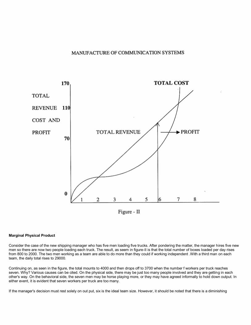
Consider the case of the new shipping manager who has five men loading five trucks. After pondering the matter, the manager hires five new men so there are now two people loading each truck. The result, as seem in figure-II is that the total number of boxes loaded per day rises from 800 to 2000. The two men working as a team are able to do more than they could if working independent .With a third man on each team, the daily total rises to 29000.

Continuing on, as seen in the figure, the total mounts to 4000 and then drops off to 3700 when the number f workers per truck reaches seven. Why? Various causes can be cited. On the physical side, there may be just too many people involved and they are getting in each other's way. On the behavioral side, the seven men may be horse playing more, or they may have agreed informally to hold down output. In either event, it is evident that seven workers per truck are too many.

If the manager's decision must rest solely on out put, six is the ideal team size. However, it should be noted that there is a diminishing

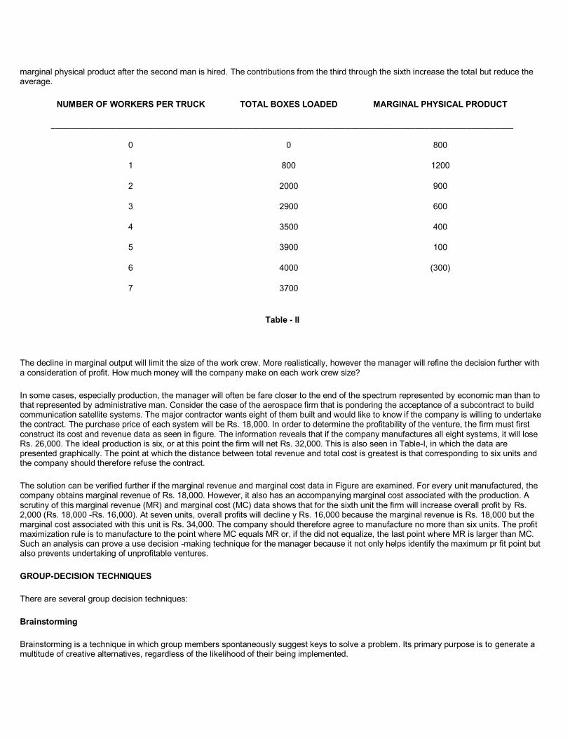
marginal physical product after the second man is hired. The contributions from the third through the sixth increase the total but reduce the average.

NUMBER OF WORKERS PER TRUCK TOTAL BOXES LOADED MARGINAL PHYSICAL PRODUCT

___________________________________________________________________________________________________

0 0 800

1 800 1200

2 2000 900

3 2900 600

4 3500 400

5 3900 100

6 4000 (300)

7 3700

Table - II

The decline in marginal output will limit the size of the work crew. More realistically, however the manager will refine the decision further with a consideration of profit. How much money will the company make on each work crew size?

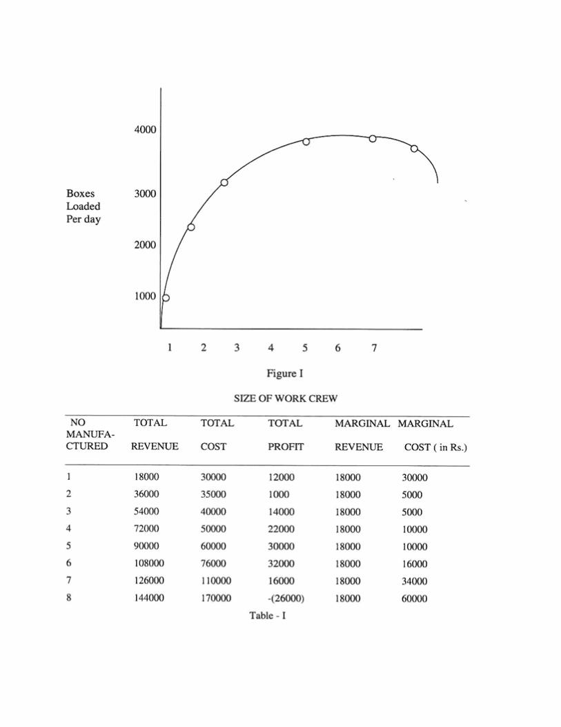
In some cases, especially production, the manager will often be fare closer to the end of the spectrum represented by economic man than to that represented by administrative man. Consider the case of the aerospace firm that is pondering the acceptance of a subcontract to build communication satellite systems. The major contractor wants eight of them built and would like to know if the company is willing to undertake the contract. The purchase price of each system will be Rs. 18,000. In order to determine the profitability of the venture, the firm must first construct its cost and revenue data as seen in figure. The information reveals that if the company manufactures all eight systems, it will lose Rs. 26,000. The ideal production is six, or at this point the firm will net Rs. 32,000. This is also seen in Table-I, in which the data are presented graphically. The point at which the distance between total revenue and total cost is greatest is that corresponding to six units and the company should therefore refuse the contract.

The solution can be verified further if the marginal revenue and marginal cost data in Figure are examined. For every unit manufactured, the company obtains marginal revenue of Rs. 18,000. However, it also has an accompanying marginal cost associated with the production. A scrutiny of this marginal revenue (MR) and marginal cost (MC) data shows that for the sixth unit the firm will increase overall profit by Rs. 2,000 (Rs. 18,000 -Rs. 16,000). At seven units, overall profits will decline y Rs. 16,000 because the marginal revenue is Rs. 18,000 but the marginal cost associated with this unit is Rs. 34,000. The company should therefore agree to manufacture no more than six units. The profit maximization rule is to manufacture to the point where MC equals MR or, if the did not equalize, the last point where MR is larger than MC. Such an analysis can prove a use decision -making technique for the manager because it not only helps identify the maximum pr fit point but also prevents undertaking of unprofitable ventures.

GROUP-DECISION TECHNIQUES

There are several group decision techniques:

Brainstorming

Brainstorming is a technique in which group members spontaneously suggest keys to solve a problem. Its primary purpose is to generate a multitude of creative alternatives, regardless of the likelihood of their being implemented.

Nominal Group Technique

The Norninal Group Technique involves, the use of highly structured meeting agenda and restricts discussion or interpersonal communication during the decision making process. While the group members are all physically present, they are required to operate independently.

Delphi Group Technique

The Delphi group Technique employs a written survey to gather expert opinions from a number of people without holding a group meeting. Unlike in brainstorming and nominal groups, Delphi group participants never meet fact to face; in fact, they may be located in different cities and never see each other.

DECISION-MAKING TOOLS

The major decision- making tools are as under:

1) Linear Programming: One of the most widely used techniques is that of linear programming. It has been described as a technique for specifying how to use limited resources or capacities of a business to obtain a particular objective, such as least cost, highest margin, or least time, when those resources have alternative uses. It is a technique that systematizes for certain conditions the process of selecting the most des able course of action from a number of available courses of action, thereby giving management information for making a more effective decision about the resources under its control. All linear programming problems must have two basic characteristics. First, two or more activities must be competing for limited resources. Second, all relationships in the problem must be linear. Linear programming can be used in the solution of many kinds of allocation decision problems, but its application is certainly limited. For example, to be employed effectively the decision problem must be formulated in quantitative terms. Nevertheless, the approach has many advantages and its application in the area of business decision making is increasing. 2) Inventory Control:

A problem faced by managers is that of maintaining adequate inventories. On the one hand, no one wants to have too many units available because there are costs associated with carrying these customer's future business.

There are two types of costs that merit the manager's consideration.

a. Clerical and Administrative costs: which are expenses associated with ordering inventory. b. Carrying costs: Carrying costs refer to the amount of money invested in the inventory, as well as other sundry expenses covering

storage space, taxes, and obsolescence.

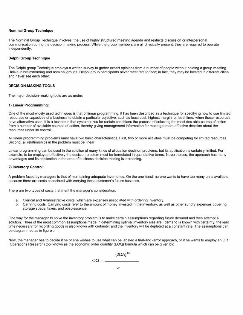
One way for the manager to solve the inventory problem is to make certain assumptions regarding future demand and then attempt a solution. Three of the most common assumptions made in determining optimal inventory size are : demand is known with certainty; the lead time necessary for recording goods is also known with certainty; and the inventory will be depleted at a constant rate. The assumptions can be diagrammed as in figure :-

Now, the manager has to decide if he or she wishes to use what can be labeled a trial-and -error approach, or if he wants to employ an OR (Operations Research) tool known as the economic order quantity (EOQ) formula which can be given by:

OQ =

{2DA}1/2 ______________

vr

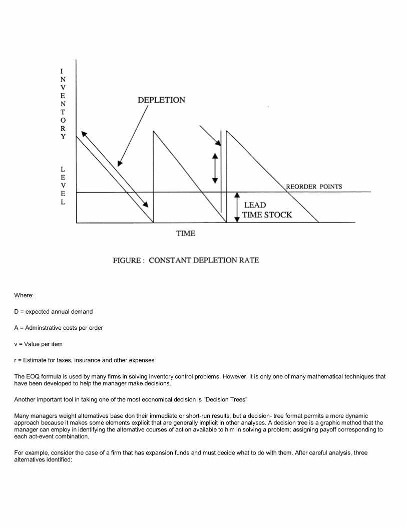
Where:

D = expected annual demand

A = Adminstrative costs per order

v = Value per item

r = Estimate for taxes, insurance and other expenses

The EOQ formula is used by many firms in solving inventory control problems. However, it is only one of many mathematical techniques that have been developed to help the manager make decisions.

Another important tool in taking one of the most economical decision is "Decision Trees"

Many managers weight alternatives base don their immediate or short-run results, but a decision- tree format permits a more dynamic approach because it makes some elements explicit that are generally implicit in other analyses. A decision tree is a graphic method that the manager can employ in identifying the alternative courses of action available to him in solving a problem; assigning payoff corresponding to each act-event combination.

For example, consider the case of a firm that has expansion funds and must decide what to do with them. After careful analysis, three alternatives identified:

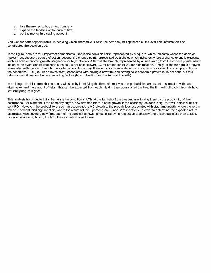
a. Use the money to buy a new company b. expand the facilities of the current firm; c. put the money in a saving account

And wait for better opportunities. In deciding which alternative is best, the company has gathered all the available information and constructed the decision tree.

In the figure there are four important components. One is the decision point, represented by a square, which indicates where the decision maker must choose a course of action. second is a chance point, represented by a circle, which indicates where a chance event is expected, such as solid economic growth, stagnation, or high inflation. A third is the branch, represented by a line flowing from the chance points, which indicates an event and its likelihood such as 0.5 per solid growth, 0.3 for stagnation or 0.2 for high inflation. Finally, at the far right is a payoff associated with the each branch. It is called a conditional payoff since its occurrence depends on certain conditions. For example, in figure the conditional ROI (Return on Investment) associated with buying a new firm and having solid economic growth is 15 per cent, but this return is conditional on the two preceding factors (buying the firm and having solid growth).

In building a decision tree, the company will start by identifying the three alternatives, the probabilities and events associated with each alternative, and the amount of return that can be expected from each. Having then constructed the tree, the firm will roll back it from right to left, analyzing as it goes.

This analysis is conducted, first by taking the conditional ROIs at the far right of the tree and multiplying them by the probability of their occurrence. For example, if the company buys a new firm and there is solid growth in the economy, as seen in figure, it will obtain a 15 per cent ROI. However, the probability of such an occurrence is 0.5 Likewise, the probabilities associated with stagnant growth, where the return will be 9 percent, and high inflation, where the return will be 3 percent, are .3 and .2 respectively. In order to determine the expected return associated with buying a new firm, each of the conditional ROIs is multiplied by its respective probability and the products are then totaled. For alternative one, buying the firm, the calculation is as follows:

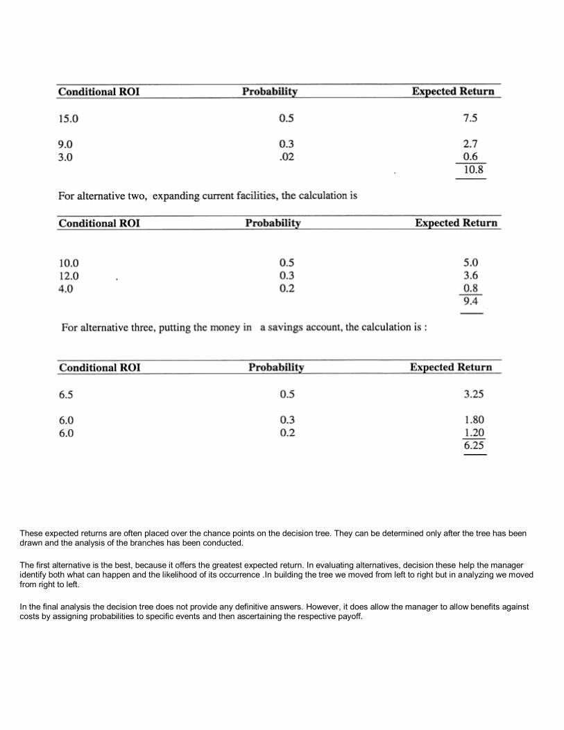
These expected returns are often placed over the chance points on the decision tree. They can be determined only after the tree has been drawn and the analysis of the branches has been conducted.

The first alternative is the best, because it offers the greatest expected return. In evaluating alternatives, decision these help the manager identify both what can happen and the likelihood of its occurrence .In building the tree we moved from left to right but in analyzing we moved from right to left.

In the final analysis the decision tree does not provide any definitive answers. However, it does allow the manager to allow benefits against costs by assigning probabilities to specific events and then ascertaining the respective payoff.

Chapter 2: DEMAND ANALYSIS

Demand can be said to be the requirement of a product by consumer (s). It is a multivariate relationship, that is , it is determined by many factors simultaneously, Some of the most important determinants of the market demand for a particular product are its own price, consumer's income, price of other commodities, consumer's tastes, income distribution, total population, consumer's wealth, credit availability, government policies, past level of demand and past level of income. The traditional theory of demand depends on four of the above determinants that are the price of the commodity, other prices, income and tastes, Demand for a commodity implies:

1. Desire to acquire it, 2. Willingness to pay for it 3. Ability to pay for it

This can be illustrated as follows. A miser's desire to acquire a product and his ability to pay for a product does not constitute a demand, as he is not willing to pay for the product. Similarly a poor man desire for a product and his willingness to pay for it is not complemented by his ability to pay for it. Hence the desire is not translated into a demand. Similarly a rich man willingness and ability to pay for a product cannot constitute a demand if he does not wish to by the product.

Thus the demand for any commodity is the desire for that commodity backed by the willingness as well as the ability to pay for it and is always defined with reference to a particular time and given values of variables on which it depends.

Types of demands

Demands for a commodity can be grouped into various categories for better understanding of its characteristics. The main categories may be:

A. Demand for consumer goods and producers goods B. Demand for perishable and durable goods C. Derived and autonomous demand D. Firm and Industry demand E. Demand by total market and industry segments

Consumer's goods and producer's goods demands

Consumer goods are those, which are, meant for the final consumption by the consumers or the end users. Producer's goods on the other hand are used for the production of consumer goods or they are intermediate goods, which are further processed upon to convert them into a form to be used by the end user. Another distinction is that the demand for producer's goods are derived demand and it indirectly depends on the demand for the consumer goods which the producer goods is used to produce. It may also be possible that this demand may be accelerated or accentuated that is I won't vary in the same proportion as the change in the demand for the final consumer goods. A small change in the demand for consumer goods may either completely wipe out the demand for the producer goods or may accelerate it.

Perishable and durable goods

Perishable (non-durable) goods are defined as those which can be used only once whereas durable goods are those which can be used over and over again. In specific cases perishable goods may also have a fixed life

span. This distinction is useful because of demand analysis. Sale of non durable goods are generally for meeting current demand whereas sale of durable goods add to the stock of existing goods whose services are used over a long period of time. Their demand is thus of two types. Replacement of old products and expansion of existing stock.

Derived and autonomous demand

When the demand for a product is tied to the demand for some parent product, then the demand is termed as derived demand. On the other hand if the demand for a commodity is completely independent of the demand of other commodities, which may be substitute or complementary or on the raw material side or on the product side, the demand for the product is termed as independent. It is very difficult to find a product whose demand is totally autonomous but some commodities like tea and vegetables do come absolute terms.

Company and Industry demand

Company demand denotes the demand for the products by a particular company or firm whereas industry demand is the demand of a product by an industry as a whole.

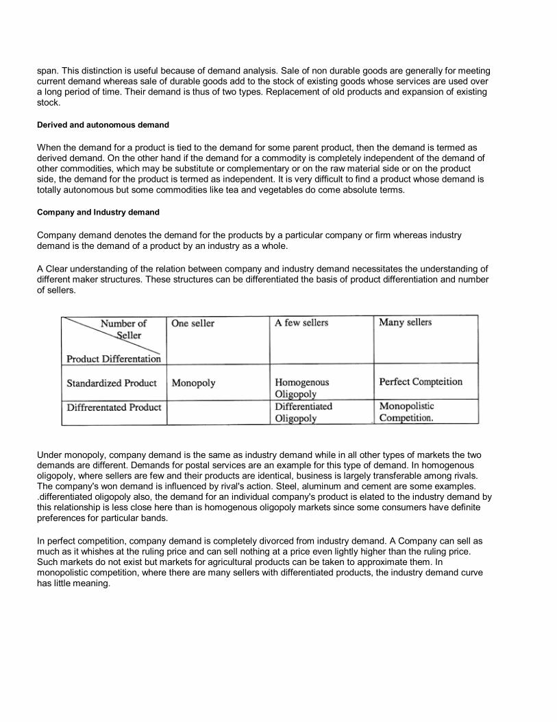
A Clear understanding of the relation between company and industry demand necessitates the understanding of different maker structures. These structures can be differentiated the basis of product differentiation and number of sellers.

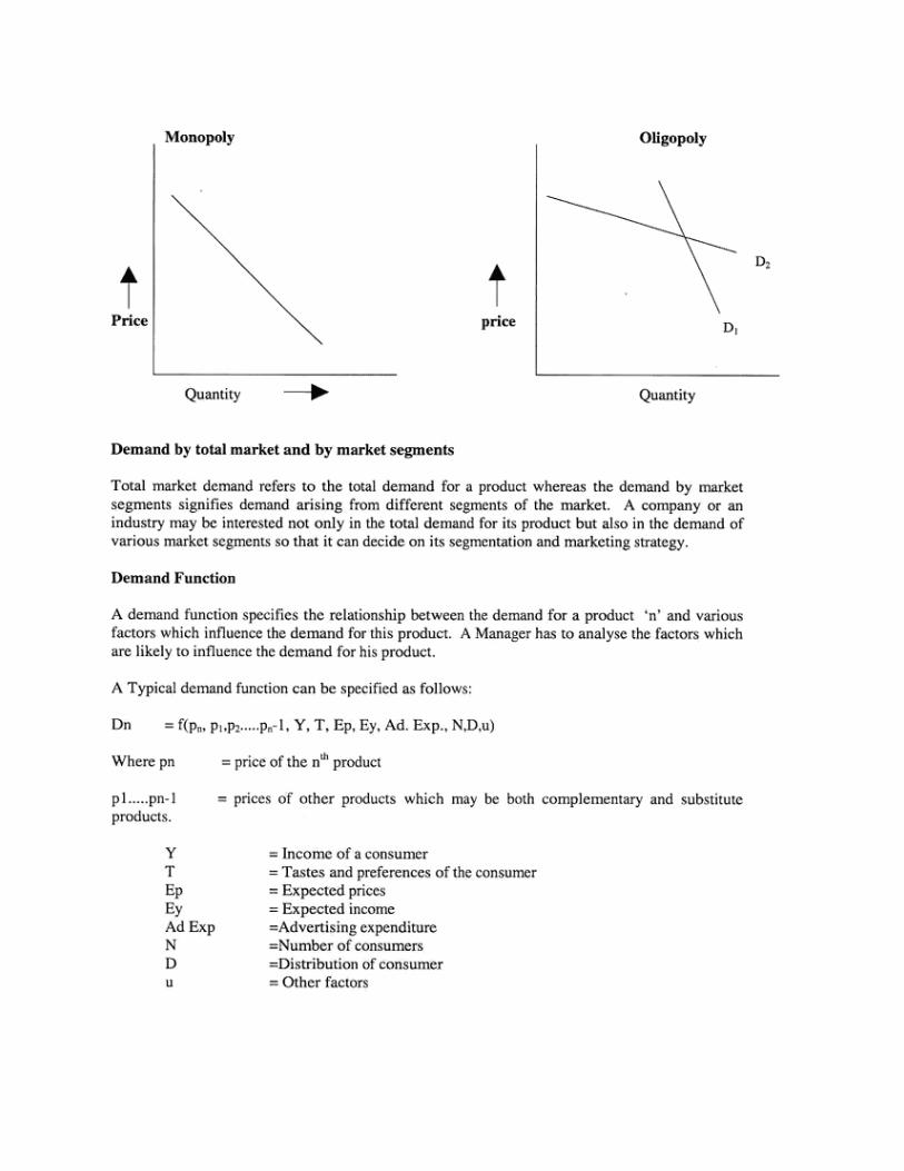
Under monopoly, company demand is the same as industry demand while in all other types of markets the two demands are different. Demands for postal services are an example for this type of demand. In homogenous oligopoly, where sellers are few and their products are identical, business is largely transferable among rivals. The company's won demand is influenced by rival's action. Steel, aluminum and cement are some examples. .differentiated oligopoly also, the demand for an individual company's product is elated to the industry demand by this relationship is less close here than is homogenous oligopoly markets since some consumers have definite preferences for particular bands.

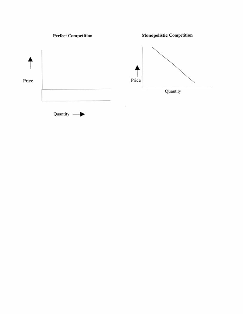
In perfect competition, company demand is completely divorced from industry demand. A Company can sell as much as it whishes at the ruling price and can sell nothing at a price even lightly higher than the ruling price. Such markets do not exist but markets for agricultural products can be taken to approximate them. In monopolistic competition, where there are many sellers with differentiated products, the industry demand curve has little meaning.

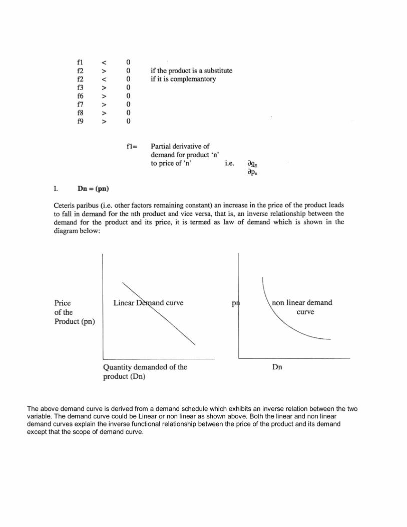
The above demand curve is derived from a demand schedule which exhibits an inverse relation between the two variable. The demand curve could be Linear or non linear as shown above. Both the linear and non linear demand curves explain the inverse functional relationship between the price of the product and its demand except that the scope of demand curve.

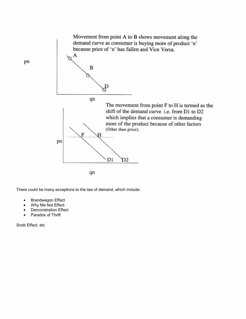
There could be many exceptions to the law of demand, which include:

Brandwagon Effect

Why Me Not Effect

Demonstration Effect

Paradox of Thrift

Snob Effect, etc.

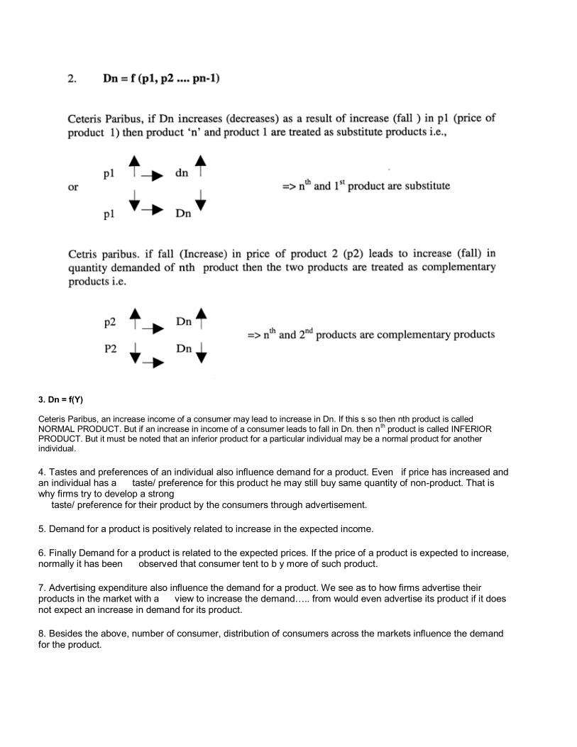
3. Dn = f(Y) Ceteris Paribus, an increase income of a consumer may lead to increase in Dn. If this s so then nth product is called NORMAL PRODUCT. But if an increase in income of a consumer leads to fall in Dn. then n

th product is called INFERIOR

PRODUCT. But it must be noted that an inferior product for a particular individual may be a normal product for another individual.

4. Tastes and preferences of an individual also influence demand for a product. Even if price has increased and an individual has a taste/ preference for this product he may still buy same quantity of non-product. That is why firms try to develop a strong taste/ preference for their product by the consumers through advertisement.

5. Demand for a product is positively related to increase in the expected income.

6. Finally Demand for a product is related to the expected prices. If the price of a product is expected to increase, normally it has been observed that consumer tent to b y more of such product.

7. Advertising expenditure also influence the demand for a product. We see as to how firms advertise their products in the market with a view to increase the demand….. from would even advertise its product if it does not expect an increase in demand for its product.

8. Besides the above, number of consumer, distribution of consumers across the markets influence the demand for the product.

It is pertinent to note that all factors which may determine demand for a product may not be known. that is why we have incorporated unknown factors,….. in our demand function.

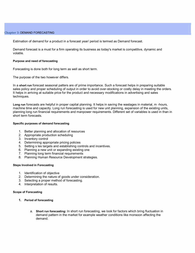
Chapter 3: DEMAND FORECASTING

Estimation of demand for a product in a forecast year/ period is termed as Demand forecast.

Demand forecast is a must for a firm operating its business as today's market is competitive, dynamic and volatile.

Purpose and need of forecasting

Forecasting is done both for long term as well as short term.

The purpose of the two however differs.

In a short run forecast seasonal patters are of prime importance. Such a forecast helps in preparing suitable sales policy and proper scheduling of output in order to avoid over-stocking or costly delay in meeting the orders. It helps in arriving at suitable price for the product and necessary modifications in advertising and sales techniques.

Long run forecasts are helpful in proper capital planning. It helps in saving the wastages in material, m -hours, machine time and capacity. Long run forecasting is used for new unit planning, expansion of the existing units, planning long run financial requirements and manpower requirements. Different set of variables is used in than in short term forecasts.

Specific purposes of demand forecasting

1. Better planning and allocation of resources 2. Appropriate production scheduling 3. Inventory control 4. Determining appropriate pricing policies 5. Setting s les targets and establishing controls and incentives. 6. Planning a new unit or expanding existing one 7. Planning long term financial requirements 8. Planning Human Resource Development strategies.

Steps Involved in Forecasting

1. Identification of objective 2. Determining the nature of goods under consideration. 3. Selecting a proper method of forecasting. 4. Interpretation of results.

Scope of Forecasting

1. Period of forecasting

a. Short run forecasting: In short run forecasting, we look for factors which bring fluctuation in demand pattern in the market for example weather conditions like monsoon affecting the demand.

b. Medium run forecasting: In medium run forecasting is done basically for timing of an activity like advertising expenditure.

c. Long run forecasting: It is done to ascertain the validity of trend. It is done for decision like diversification.

2. Levels of Forecasting

a. Macroeconomic forecasting is concerned with business conditions of the whole economy. It is measured with the help of indices like wholesale price index, consumer price index.

b. Industry demand forecasting gives indication to firm regarding direction in which the whole industry will be moving. It is used to decide the way the firm should plan for future in relation to the industry.

c. Firm demand forecasting is done for planning companies overall operations like sales forecasting etc.

d. Product line forecasting helps the firm to decide which of the product or products should have priority in the allocation of firm's limited resources.

3. General purpose or specific purpose forecast helps the firm in taking general factors into consideration while forecasting for demand.

4. Forecast of established product or a new product

5. Types of commodity for which forecast is to be done. Goods can be broadly classified into capital goods, consumer durable and non-durable consumer goods. For each of these categories of goods there is a distinctive pattern of demand.

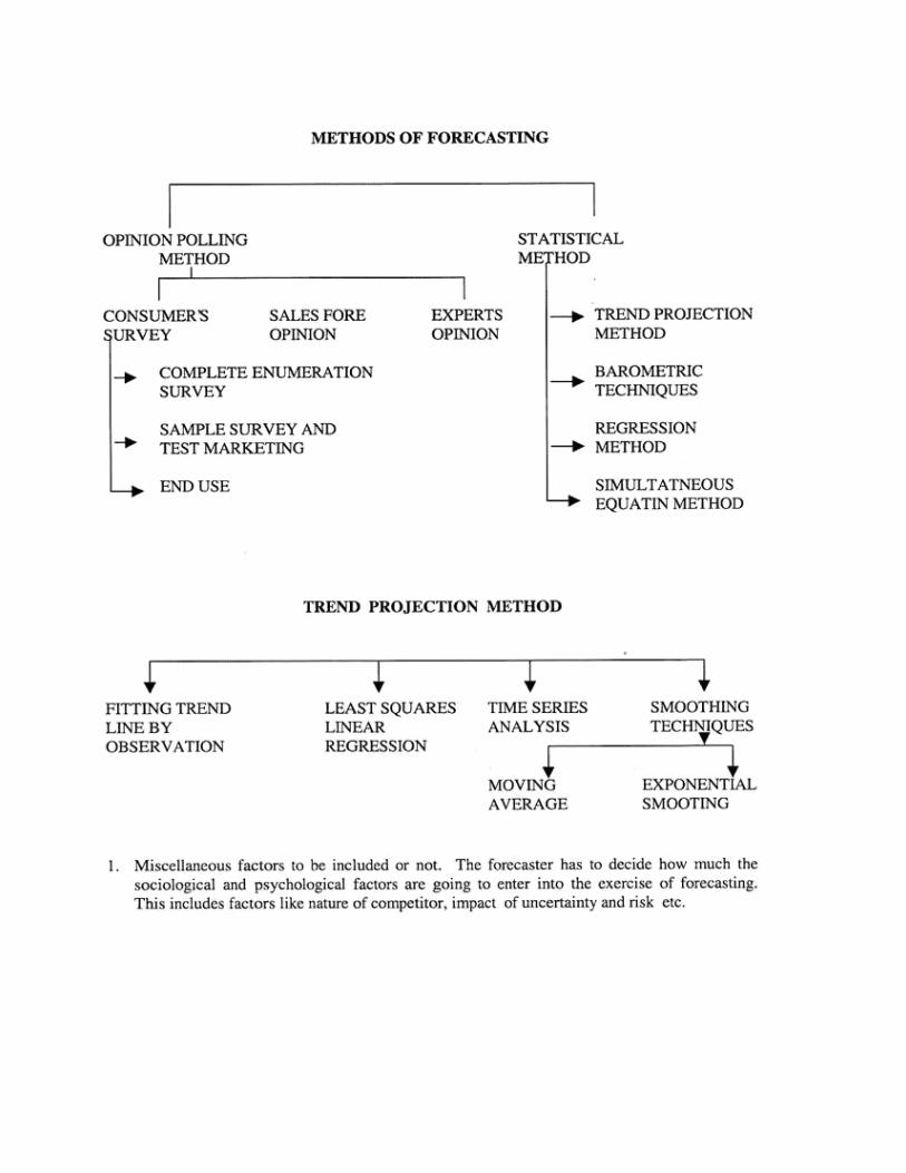
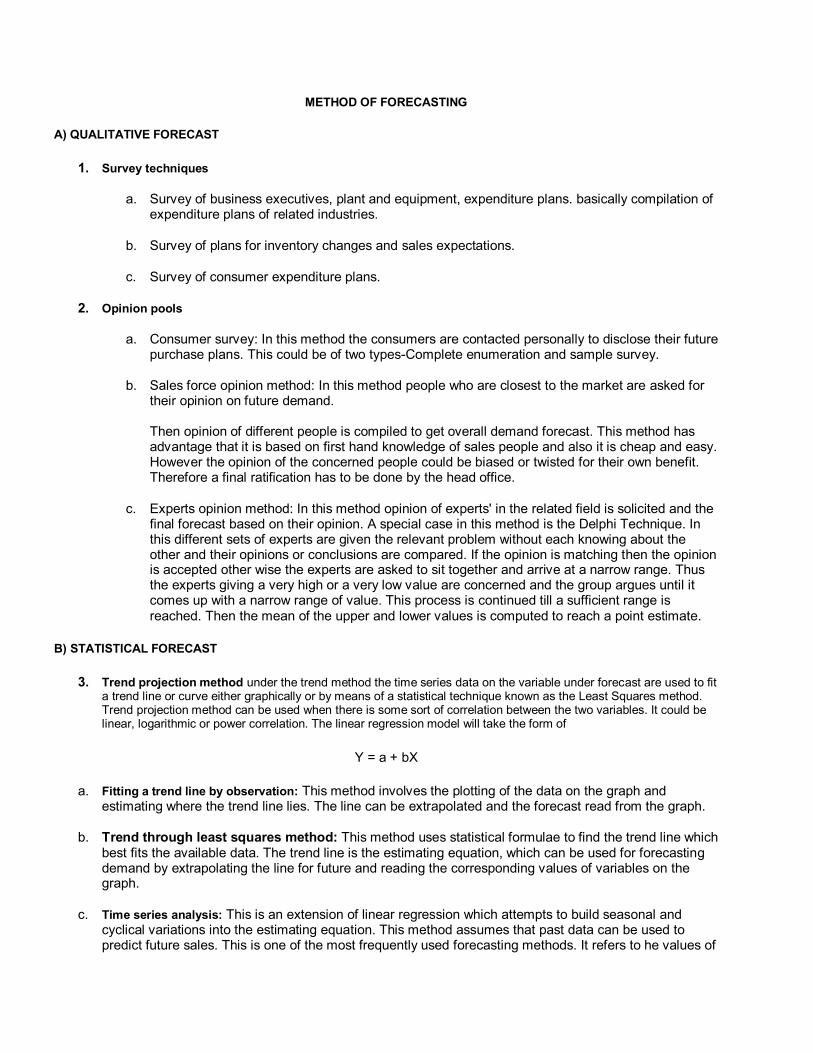
METHOD OF FORECASTING

A) QUALITATIVE FORECAST

1. Survey techniques

a. Survey of business executives, plant and equipment, expenditure plans. basically compilation of expenditure plans of related industries.

b. Survey of plans for inventory changes and sales expectations.

c. Survey of consumer expenditure plans.

2. Opinion pools

a. Consumer survey: In this method the consumers are contacted personally to disclose their future purchase plans. This could be of two types-Complete enumeration and sample survey.

b. Sales force opinion method: In this method people who are closest to the market are asked for their opinion on future demand. Then opinion of different people is compiled to get overall demand forecast. This method has advantage that it is based on first hand knowledge of sales people and also it is cheap and easy. However the opinion of the concerned people could be biased or twisted for their own benefit. Therefore a final ratification has to be done by the head office.

c. Experts opinion method: In this method opinion of experts' in the related field is solicited and the final forecast based on their opinion. A special case in this method is the Delphi Technique. In this different sets of experts are given the relevant problem without each knowing about the other and their opinions or conclusions are compared. If the opinion is matching then the opinion is accepted other wise the experts are asked to sit together and arrive at a narrow range. Thus the experts giving a very high or a very low value are concerned and the group argues until it comes up with a narrow range of value. This process is continued till a sufficient range is reached. Then the mean of the upper and lower values is computed to reach a point estimate.

B) STATISTICAL FORECAST

3. Trend projection method under the trend method the time series data on the variable under forecast are used to fit a trend line or curve either graphically or by means of a statistical technique known as the Least Squares method. Trend projection method can be used when there is some sort of correlation between the two variables. It could be linear, logarithmic or power correlation. The linear regression model will take the form of

Y = a + bX

a. Fitting a trend line by observation: This method involves the plotting of the data on the graph and estimating where the trend line lies. The line can be extrapolated and the forecast read from the graph.

b. Trend through least squares method: This method uses statistical formulae to find the trend line which best fits the available data. The trend line is the estimating equation, which can be used for forecasting demand by extrapolating the line for future and reading the corresponding values of variables on the graph.

c. Time series analysis: This is an extension of linear regression which attempts to build seasonal and cyclical variations into the estimating equation. This method assumes that past data can be used to predict future sales. This is one of the most frequently used forecasting methods. It refers to he values of

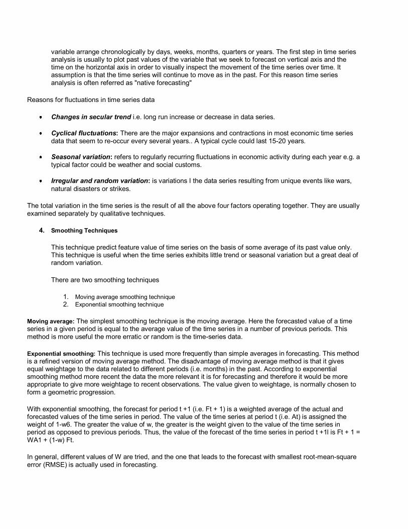
variable arrange chronologically by days, weeks, months, quarters or years. The first step in time series analysis is usually to plot past values of the variable that we seek to forecast on vertical axis and the time on the horizontal axis in order to visually inspect the movement of the time series over time. It assumption is that the time series will continue to move as in the past. For this reason time series analysis is often referred as "native forecasting"

Reasons for fluctuations in time series data

Changes in secular trend i.e. long run increase or decrease in data series.

Cyclical fluctuations: There are the major expansions and contractions in most economic time series data that seem to re-occur every several years.. A typical cycle could last 15-20 years.

Seasonal variation: refers to regularly recurring fluctuations in economic activity during each year e.g. a typical factor could be weather and social customs.

Irregular and random variation: is variations I the data series resulting from unique events like wars,

natural disasters or strikes.

The total variation in the time series is the result of all the above four factors operating together. They are usually examined separately by qualitative techniques.

4. Smoothing Techniques

This technique predict feature value of time series on the basis of some average of its past value only. This technique is useful when the time series exhibits little trend or seasonal variation but a great deal of random variation.

There are two smoothing techniques

1. Moving average smoothing technique 2. Exponential smoothing technique

Moving average: The simplest smoothing technique is the moving average. Here the forecasted value of a time series in a given period is equal to the average value of the time series in a number of previous periods. This method is more useful the more erratic or random is the time-series data.

Exponential smoothing: This technique is used more frequently than simple averages in forecasting. This method is a refined version of moving average method. The disadvantage of moving average method is that it gives equal weightage to the data related to different periods (i.e. months) in the past. According to exponential smoothing method more recent the data the more relevant it is for forecasting and therefore it would be more appropriate to give more weightage to recent observations. The value given to weightage, is normally chosen to form a geometric progression.

With exponential smoothing, the forecast for period t +1 (i.e. Ft + 1) is a weighted average of the actual and forecasted values of the time series in period. The value of the time series at period t (i.e. At) is assigned the weight of 1-w6. The greater the value of w, the greater is the weight given to the value of the time series in period as opposed to previous periods. Thus, the value of the forecast of the time series in period t +1l is Ft + 1 = WA1 + (1-w) Ft.

In general, different values of W are tried, and the one that leads to the forecast with smallest root-mean-square error (RMSE) is actually used in forecasting.

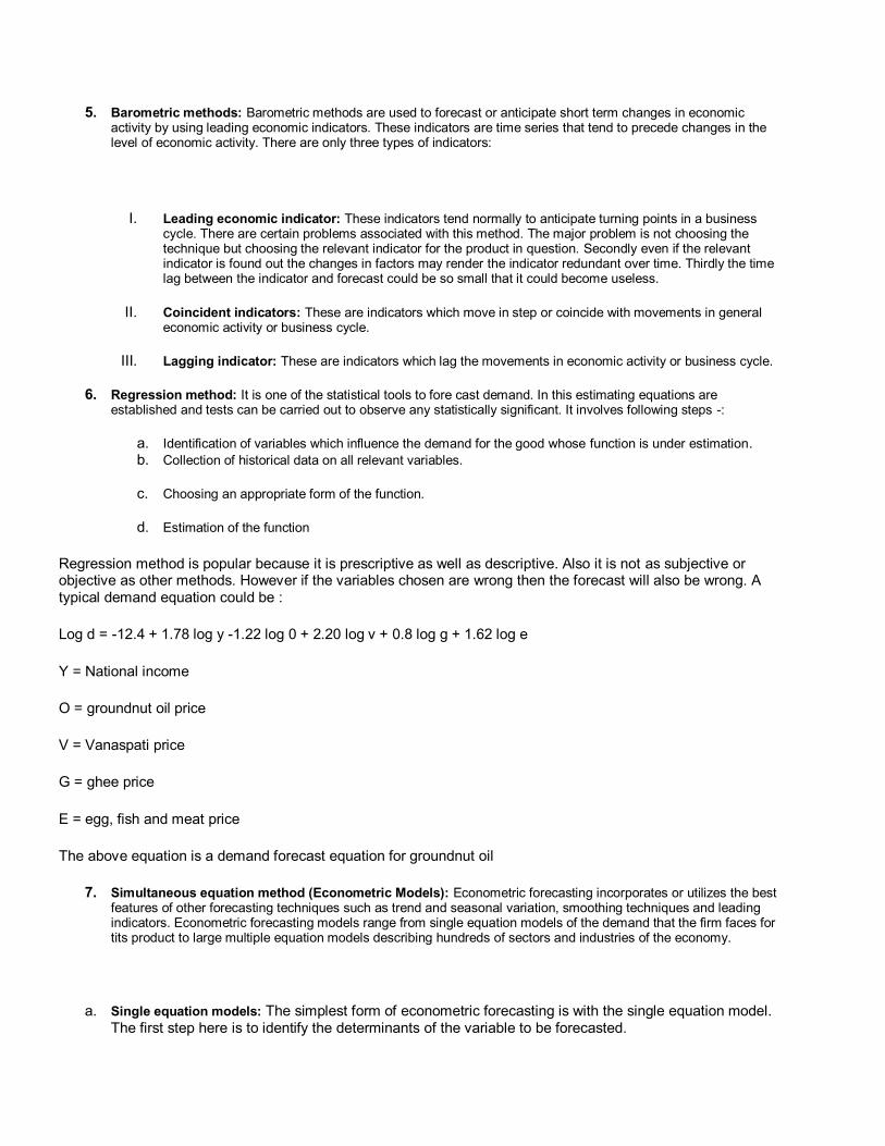
5. Barometric methods: Barometric methods are used to forecast or anticipate short term changes in economic activity by using leading economic indicators. These indicators are time series that tend to precede changes in the level of economic activity. There are only three types of indicators:

I. Leading economic indicator: These indicators tend normally to anticipate turning points in a business cycle. There are certain problems associated with this method. The major problem is not choosing the technique but choosing the relevant indicator for the product in question. Secondly even if the relevant indicator is found out the changes in factors may render the indicator redundant over time. Thirdly the time lag between the indicator and forecast could be so small that it could become useless.

II. Coincident indicators: These are indicators which move in step or coincide with movements in general economic activity or business cycle.

III. Lagging indicator: These are indicators which lag the movements in economic activity or business cycle.

6. Regression method: It is one of the statistical tools to fore cast demand. In this estimating equations are established and tests can be carried out to observe any statistically significant. It involves following steps -:

a. Identification of variables which influence the demand for the good whose function is under estimation. b. Collection of historical data on all relevant variables.

c. Choosing an appropriate form of the function.

d. Estimation of the function

Regression method is popular because it is prescriptive as well as descriptive. Also it is not as subjective or objective as other methods. However if the variables chosen are wrong then the forecast will also be wrong. A typical demand equation could be :

Log d = -12.4 + 1.78 log y -1.22 log 0 + 2.20 log v + 0.8 log g + 1.62 log e

Y = National income

O = groundnut oil price

V = Vanaspati price

G = ghee price

E = egg, fish and meat price

The above equation is a demand forecast equation for groundnut oil

7. Simultaneous equation method (Econometric Models): Econometric forecasting incorporates or utilizes the best features of other forecasting techniques such as trend and seasonal variation, smoothing techniques and leading indicators. Econometric forecasting models range from single equation models of the demand that the firm faces for tits product to large multiple equation models describing hundreds of sectors and industries of the economy.

a. Single equation models: The simplest form of econometric forecasting is with the single equation model. The first step here is to identify the determinants of the variable to be forecasted.

Q = a0 + a1P + a2Y +a3N + a4P5 + a5Pc + a6a + e Q = demand

P = Price

Y = disposable income

N = size of population

Ps = price of a substitute

Pc = price of complement A = level of advertising by the firm

b. Multiple equation model: Sometimes economic relationships may be so complex that a multiple equation model may be required. This is particularly used in forecasting micro variables or the demand and sales of major sectors or industries. Multiple equation model for GNP-:

Ct = a1+b1GNPt+u1t It =a2+b2IIt-1+U2t GNPt= Ct+ It+Gt

C = consumption expenditures

GNP = Gross national product in year t

I = investment

II = Profit

G = Government expenditures

U = stochastic disturbance (random error term)

T = current year

t-1 = previous year

Variables to the left of the equal sign are called endogenous variable. These are the variables that the model seeks to explain or predict from the solution of the model. Exogenous variables are those determinants outside the model or right of the equal sign of the equation.

8. Input Output Forecasting

Input output analysis was introduced by Prof. Leontief. With this technique the firm can also forecast using Input output tables. It shows the use of the output of each industry as input by other industries and for final consumption. Input and output analysis allow us to trace through all these inter industry input and outputs flow though out the economy and to determine the total increase of all the inputs required to meet the increased demand. In this technique we have two input output matrixes

1. Direct requirement matrix 2. Total requirement matrix

Uses and Shortcomings of input-output forecasting

Input-output analysis and forecasting has many uses and applications. It is used by the firm to forecast the raw material, labour, and capital requirement needed to meet the forecasted change in the demand for their product.

Shortcomings:

1. The direct and total requirement coefficient are assumed to be fixed and thus do not allow input substitution.

2. Input output tales are usually available with a time lag of many years and while the input output coefficient do not change very rapidly over the course of many years they can become very biased.

RISKS IN DEMAND FORECASTING

Demand forecasting faces two major risks.

1. Overestimating demand 2. Underestimating demand

One risk arises from entirely unforeseen events such as war, political upheavals and natural disasters.

The second risk arises from inadequate analysis of the market.

All these costly forecasting errors could possibly have been avoided.

a. Carefully defining the market for the product to include all potential users of the market and considering the possibility of product substitution

b. Dividing total industry demand into its components and analyzing each component separately. c. Forecasting the main driver or user of the product in each segment of the market and projecting how

they are likely to change in the future.

Conducting sensitivity analysis of how the forecast would be affected by change in any of the assumption on

which the forecast is based.

The physical conditions of production, the price of resources and the economically efficient conduct of an entrepreneur jointly determine the cost of production of a business.

Apart from being determined by other exogenous variables, the output level of a firm is also determined by the cost of producing the desired level of output. A firm aims at operating in a situation where revenues are maximum and costs are minimum. It would also like to produce a that optimal out put where it gets a maximum profit as determined by the difference between cost and revenue. Hence it is important to analyze the cost output relationship.

COST CONCEPTS

The most widely accepted concept is the money cost of production. It means the aggregate money expenditure by a firm on various items required in the production of a commodity. For example expenditure on raw materials purchased salary & wages paid to the employees etc.

There are several useful cost concepts and clear understanding of them is necessary for cost analysis:

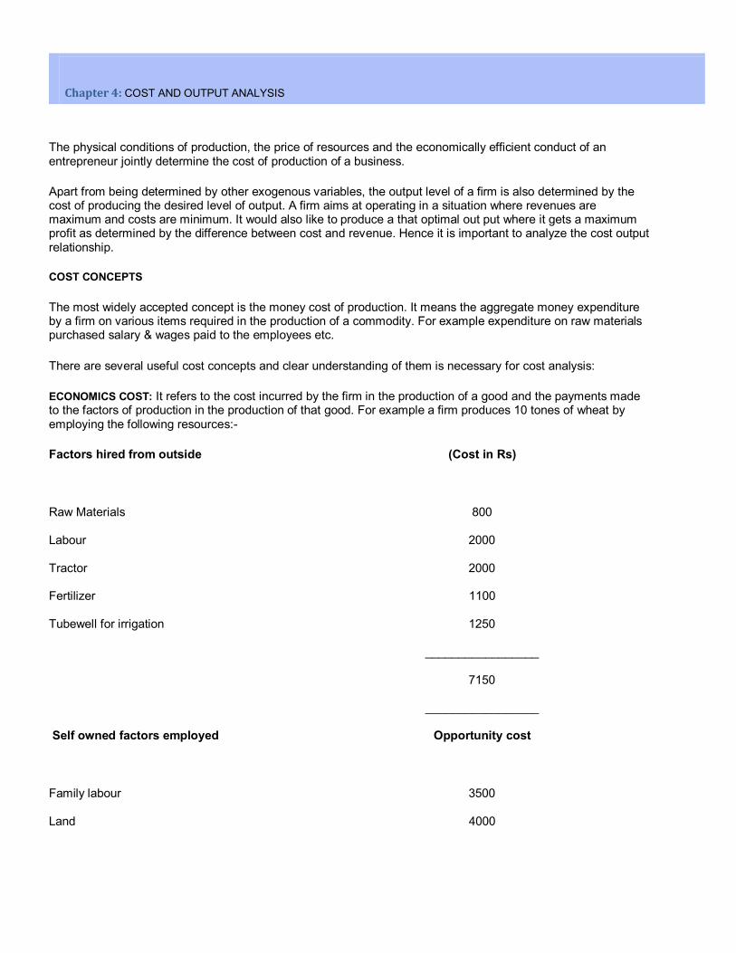
ECONOMICS COST: It refers to the cost incurred by the firm in the production of a good and the payments made to the factors of production in the production of that good. For example a firm produces 10 tones of wheat by employing the following resources:-

Factors hired from outside (Cost in Rs)

Raw Materials 800

Labour 2000

Tractor 2000

Fertilizer 1100

Tubewell for irrigation 1250

_________________

7150

_________________

Self owned factors employed Opportunity cost

Family labour 3500

Land 4000

Chapter 4: COST AND OUTPUT ANALYSIS

_________________

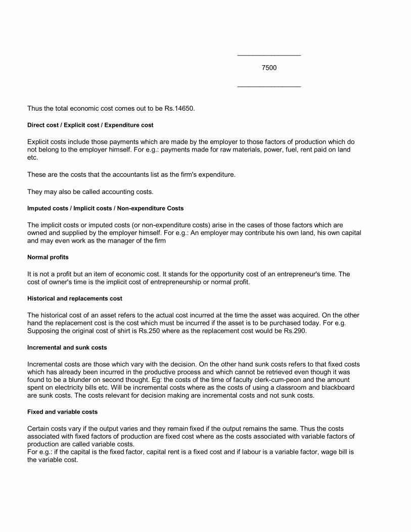
7500

_________________

Thus the total economic cost comes out to be Rs.14650.

Direct cost / Explicit cost / Expenditure cost

Explicit costs include those payments which are made by the employer to those factors of production which do not belong to the employer himself. For e.g.: payments made for raw materials, power, fuel, rent paid on land etc.

These are the costs that the accountants list as the firm's expenditure.

They may also be called accounting costs.

Imputed costs / Implicit costs / Non-expenditure Costs

The implicit costs or imputed costs (or non-expenditure costs) arise in the cases of those factors which are owned and supplied by the employer himself. For e.g.: An employer may contribute his own land, his own capital and may even work as the manager of the firm

Normal profits

It is not a profit but an item of economic cost. It stands for the opportunity cost of an entrepreneur's time. The cost of owner's time is the implicit cost of entrepreneurship or normal profit.

Historical and replacements cost

The historical cost of an asset refers to the actual cost incurred at the time the asset was acquired. On the other hand the replacement cost is the cost which must be incurred if the asset is to be purchased today. For e.g. Supposing the original cost of shirt is Rs.250 where as the replacement cost would be Rs.290.

Incremental and sunk costs

Incremental costs are those which vary with the decision. On the other hand sunk costs refers to that fixed costs which has already been incurred in the productive process and which cannot be retrieved even though it was found to be a blunder on second thought. Eg: the costs of the time of faculty clerk-cum-peon and the amount spent on electricity bills etc. Will be incremental costs where as the costs of using a classroom and blackboard are sunk costs. The costs relevant for decision making are incremental costs and not sunk costs.

Fixed and variable costs

Certain costs vary if the output varies and they remain fixed if the output remains the same. Thus the costs associated with fixed factors of production are fixed cost where as the costs associated with variable factors of production are called variable costs. For e.g.: if the capital is the fixed factor, capital rent is a fixed cost and if labour is a variable factor, wage bill is the variable cost.

Opportunity cost

It refers to the cost of producing a particular product which is the value of the other products that the resources used in its production could have produced instead. For e.g.: The cost of producing locomotives is the value of the goods and services that could have been obtained from the manpower, equipment, and the materials used currently in locomotive production.

Separable and common costs

Costs are classified on their basis of their traceability. The costs, which can be attributed to a product, a department or a process, are the separable costs and the rests are non- -separable or common costs. Eg: IN a multi-product firm raw materials cost is a separable product wise but the management cost is not separable that way.

Social and private costs

Private costs refer to the costs incurred by an individual firm while social costs stand for the costs incurred by the society as a whole. The former is the sum total of explicit and implicit costs that a firm incurs in the production. But since managerial economics deals primarily with decision making by a firm only economic costs are relevant.

Total. Average and marginal costs

The three concepts of total, average and marginal costs on the supply side are the counterparts of the total, average and marginal revenue on the demand side. Total cost is the total money cost of production of a commodity. The average cost is obtained by dividing total cost of production by the number of units of the commodity reduced so that

Average Cost =

Total Cost _________

Output

Marginal cost is the cost of producing the final or the marginal unit of the commodity. Alternately it may be expressed as the total cost of n units of the output minus the total cost of n-1units. Both average as well as the marginal cost curves are normally U- shaped curves. As long as average cost curve (AC) is falling the marginal cost (MC) curve is below it. Likewise, when the average cost curve starts rising, the marginal cost curve is above it.

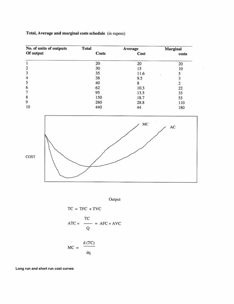
Long run and short run cost curves

Long run costs and short run costs are related to long and short run production functions. In the long run all costs are variable costs while in the short run, some costs are fixed and some are variable. Combining this classification with the earlier one between the total, marginal and average costs, there are three long run cost concepts and seven short run ones. The former consists of the long run total costs (LTC)., long run average costs (LAC) and long run marginal cost (LMC), and the latter comprises of short run average fixed cost (AFC), short run total variable cost (TVC) and short run average cost (AVC). Hence,

STC = TFC + TVD

SAC = AFC + AVC

Both long run and short run costs are useful for decision making. In the long run, a fIrm is concerned with optimum output within a given plant size.

COST FUNCTION:

Cost functions are derived functions. They are derived from the production function which describes the available efficient methods of production at any point of time.

Both in the short run and in the long run, total cost is a multivariate function. That is total cost is determined by many factors. Symbolically we may write the long run cost function as

C = f (X, T, Pf)

And the short run cost function as

C = f(X, T, Pf, K)

Where C = Total Cost

X = Output

T = Technology

Pf = Price of Factors

K = Fixed Factors

Graphically these are shown on two dimensional diagrams. Such curves imply that cost is a function of output, C = f (X) ceteris paribus of the three, sets of cost determinants, output assumes a special role. This is for two reasons. One, output is the only variable which is under the direct control of the firm .Two, the relationship between total cost and output is unique.

SHORT RUN COST CURVES

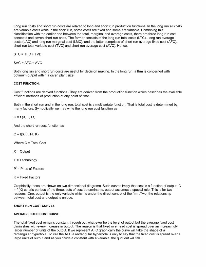
AVERAGE FIXED COST CURVE

The total fixed cost remains constant through out what ever be the level of output but the average fixed cost diminishes with every increase in output. The reason is that fixed overhead cost is spread over an increasingly larger number of units of the output. If we represent AFC graphically the curve will take the shape of a rectangular hyperbola. To call the AFC a rectangular hyperbola is only to say that the fixed cost is spread over a large units of output and as you divide a constant with a variable, the quotient will fall. .

The AFC curve falls steeply in the beginning and tends towards touching the horizontal axis though it never succeeds in doing so.Thus, it is evident that units with large fixed costs, for example the railways with huge fixed expenditure on the rail track can cut down on their average fixed costs by going in for a larger output.

AVERAGE VARIABLE COST CURVE:

As shown in column 6 in the foregoing schedule the total variable cost increases with every increase in the output of the firm the reason being that more labor is with every increase in the output of the firm. The average variable cost declines in the beginning up-to a certain point and then starts rising sharply after that point. The shape of the AVC curve is shown as below.

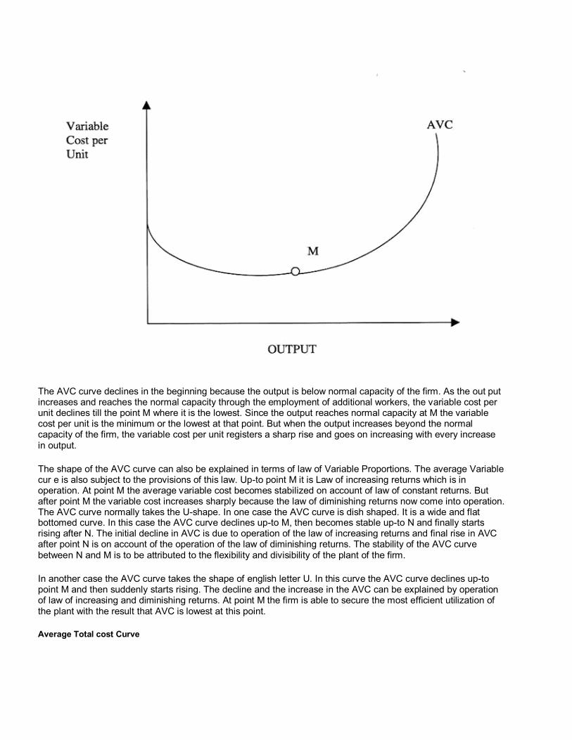
The AVC curve declines in the beginning because the output is below normal capacity of the firm. As the out put increases and reaches the normal capacity through the employment of additional workers, the variable cost per unit declines till the point M where it is the lowest. Since the output reaches normal capacity at M the variable cost per unit is the minimum or the lowest at that point. But when the output increases beyond the normal capacity of the firm, the variable cost per unit registers a sharp rise and goes on increasing with every increase in output.

The shape of the AVC curve can also be explained in terms of law of Variable Proportions. The average Variable cur e is also subject to the provisions of this law. Up-to point M it is Law of increasing returns which is in operation. At point M the average variable cost becomes stabilized on account of law of constant returns. But after point M the variable cost increases sharply because the law of diminishing returns now come into operation. The AVC curve normally takes the U-shape. In one case the AVC curve is dish shaped. It is a wide and flat bottomed curve. In this case the AVC curve declines up-to M, then becomes stable up-to N and finally starts rising after N. The initial decline in AVC is due to operation of the law of increasing returns and final rise in AVC after point N is on account of the operation of the law of diminishing returns. The stability of the AVC curve between N and M is to be attributed to the flexibility and divisibility of the plant of the firm.

In another case the AVC curve takes the shape of english letter U. In this curve the AVC curve declines up-to point M and then suddenly starts rising. The decline and the increase in the AVC can be explained by operation of law of increasing and diminishing returns. At point M the firm is able to secure the most efficient utilization of the plant with the result that AVC is lowest at this point.

Average Total cost Curve

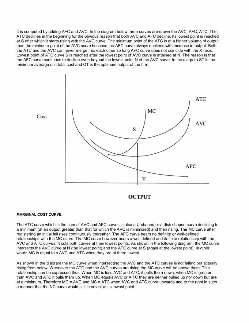
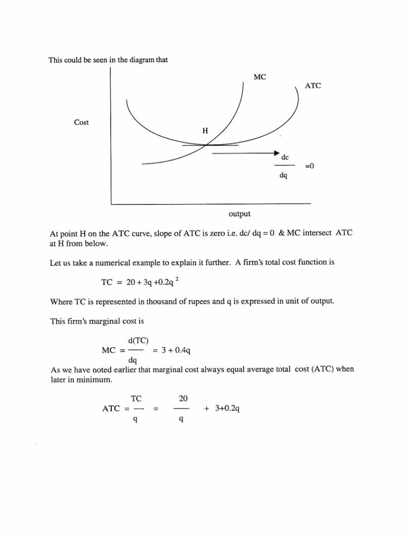
It is computed by adding AFC and AVC. In the diagram below three curves are drawn the AVC, AFC, ATC. The ATC declines in the beginning for the obvious reason that both AVC and AFC decline. Its lowest point is reached at S after which it starts rising with the AVC curve. The minimum point of the ATC is at a higher volume of output than the minimum point of the AVC curve because the AFC curve always declines with increase in output. Both the ATC and the AVC can never merge into each other so long AFC curve does not coincide with the X -axis. Lowest point of ATC curve S is reached after the lowest point of AVC curve is attained at N. The reason is that the AFC curve continues to decline even beyond the lowest point N of the AVC curve. In the diagram ST is the minimum average unit total cost and OT is the optimum output of the fIrm.

MARGINAL COST CURVE:

The ATC curve which is the sum of AVC and AFC curves is also a U-shaped or a dish shaped curve declining to a minimum (at an output greater than that for which the AVC is minimized) and then rising. The MC curve after registering an initial fall rises continuously thereafter. The AFC curve bears no definite or well-defined relationships with the MC curve. The MC curve however bears a well defined and definite relationship with the AVC and ATC curves. It cuts both curves at their lowest points. As shown in the following diagram, the MC curve intersects the AVC curve at N (the lowest point) and the ATC curve at S (again at the lowest point). In other words MC is equal to a AVC and ATC when they are at there lowest.

As shown in the diagram the MC curve when intersecting the AVC and the ATC curves is not falling but actually rising from below. Whenever the ATC and the AVC curves are rising the MC curve will be above them. This relationship can be expressed thus. When MC is less AVC and ATC, it pulls them down, when MC is greater than AVC and ATC it pulls them up. When MC equals AVC or A TC they are neither pulled up nor down but are at a minimum, Therefore MC = AVC and MC = ATC when AVC and ATC curve upwards and to the right in such a manner that the NC curve would still intersect at its lowest point.

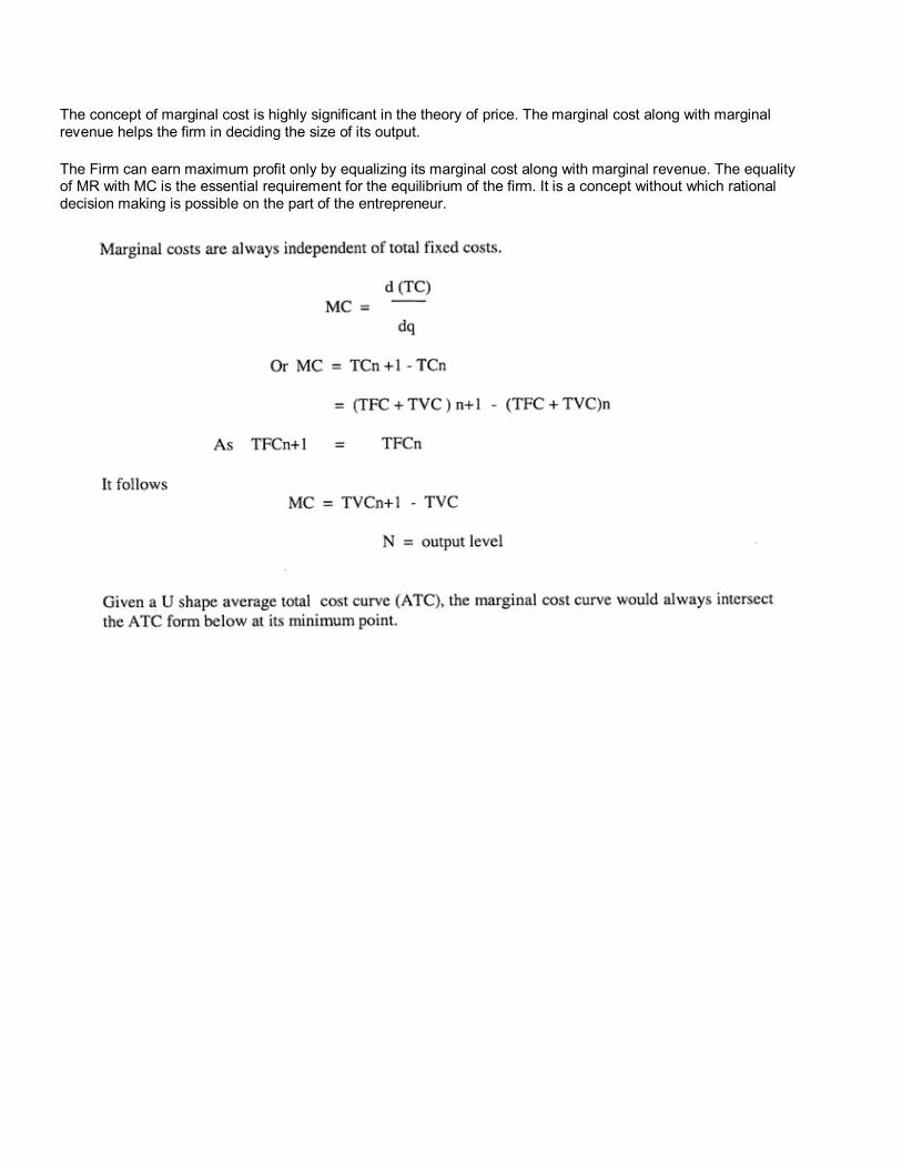
The concept of marginal cost is highly significant in the theory of price. The marginal cost along with marginal revenue helps the firm in deciding the size of its output.

The Firm can earn maximum profit only by equalizing its marginal cost along with marginal revenue. The equality of MR with MC is the essential requirement for the equilibrium of the firm. It is a concept without which rational decision making is possible on the part of the entrepreneur.

LONG RUN COST CURVE In the short period the firm does not have adequate time to change the size of its plant or the scale of its operations, But in the long period there is no such difficulty. If the demand for the firm's product increases, the firm can increase its output by enlarging the size of its plant or increasing the scale of its operations.

All the factors are variable, none is fixed. Hence, there is no need; of an average fixed cost curves in the long period. The long run cost curves are also, like the short run cost curves, U shaped. The only difference is that the long run cost curves are flatter than the short run cost curves, or the U shape of the long run cost curves is less pronounced than that of short run cost curves.

Let us now take up the more advanced explanation why the U-shape of the long run cost curves is less pronounced compared with the U shape of the short run cost curves. In the short period, as we have already seen as machinery and management are indivisible.

On account of the availability of adequate time, the size of these factors (say machinery and management) can be altered in the long run so that they can be used in differing proportions for the purpose of production. These factors do not therefore remain completely indivisible in the long run.

Since all factors of production (including machinery and management) can be used in variable proportions in the long run, it is possible for the firm to alter its scale of operations in accordance with the requirements of output.

In the diagram we have drawn three short run average cost curves namely SRAC. SRAC and SRAC respectively, corresponding to the three scales of operations possible in the long period. Suppose the firm is producing according to the scale of operations represented by SRAC. In this case the firm will produce OM output because this represents optimum output.

With the existing scale of operations but at a higher average cost, namely M'" K'" cost. But if the firm were producing in the long period and had enough time at its disposal to change the scale 'of operations, it could obtain the same output, i.e. OM'" output at a lower average cost of M'" L "'.

By varying the size of the plant and also the scale of its operations, the firm can produce a given output at a lower average cost in the long than in the short run. For each different scale of operations, there will be an output where average cost is the lowest. This will be indicated by the lowest point on the relevant short run average cost curve. Such an output is termed as optimum output. For example for SRAC', OM' is the optimum output. Likewise for SRAC"'m OM'" is the optimum output.

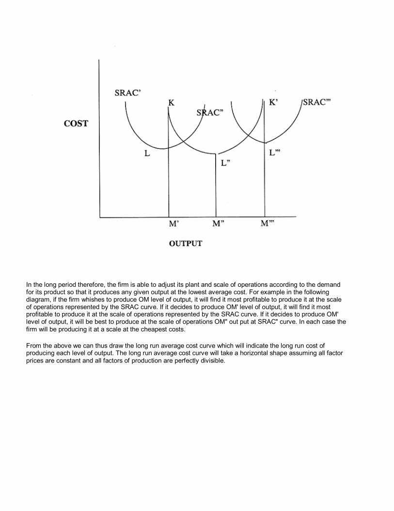
In the long period therefore, the firm is able to adjust its plant and scale of operations according to the demand for its product so that it produces any given output at the lowest average cost. For example in the following diagram, if the firm whishes to produce OM level of output, it will find it most profitable to produce it at the scale of operations represented by the SRAC curve. If it decides to produce OM' level of output, it will find it most profitable to produce it at the scale of operations represented by the SRAC curve. If it decides to produce OM' level of output, it will be best to produce at the scale of operations OM" out put at SRAC" curve. In each case the firm will be producing it at a scale at the cheapest costs.

From the above we can thus draw the long run average cost curve which will indicate the long run cost of producing each level of output. The long run average cost curve will take a horizontal shape assuming all factor prices are constant and all factors of production are perfectly divisible.

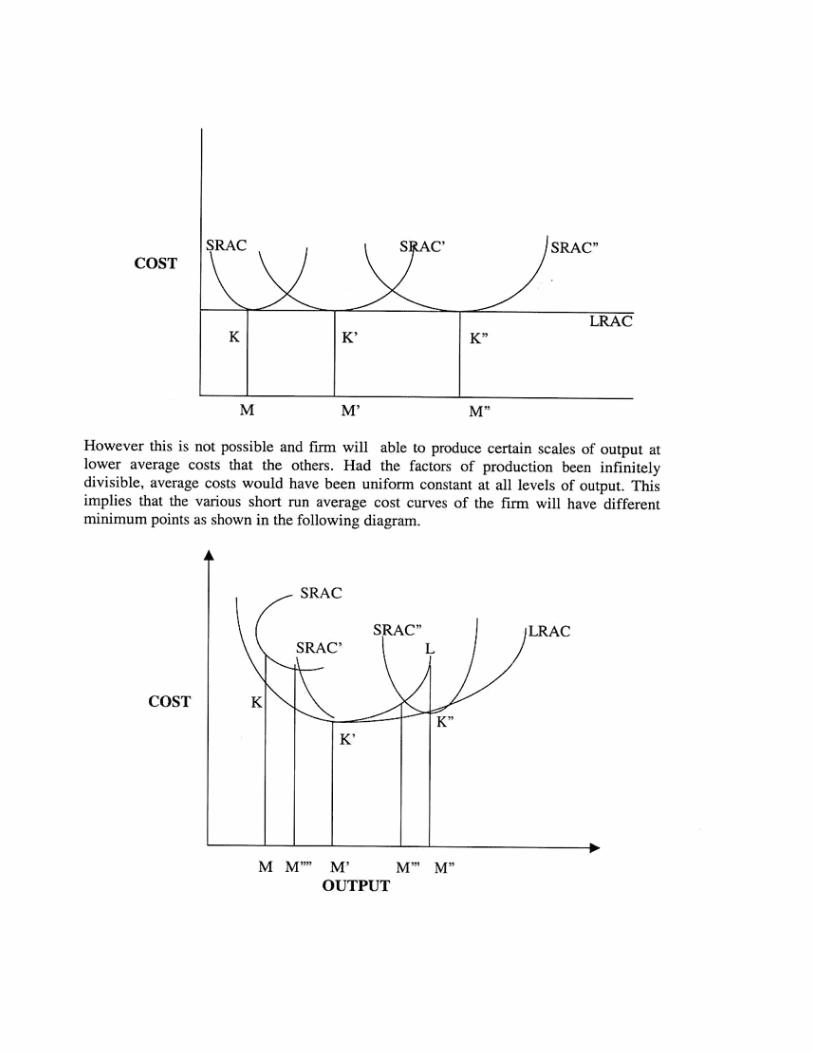
In the above diagram the curve SRAC' has a lower minimum point at K' at either the curve SRAC or the curve SRAC". OM' constitutes the optimum output of curve SRAC'. The LRAC is the long run average cost curves. It is tangent to all the SRAC curves at different points. It is tangent to SRAC at K. SRAC' at K' and SRAC" at K". The LRAC curve is U-shaped though it U shape is not as pronounced as the SRAC curves. It is flatter than the SRAC curve and is also known as the envelope curve as it envelopes all the SRAC. The LRAC is also called the planning curve as it represents the cost output data which are useful to the firm when it is formulating its policy with regard to its scale of operations over a long period of time.

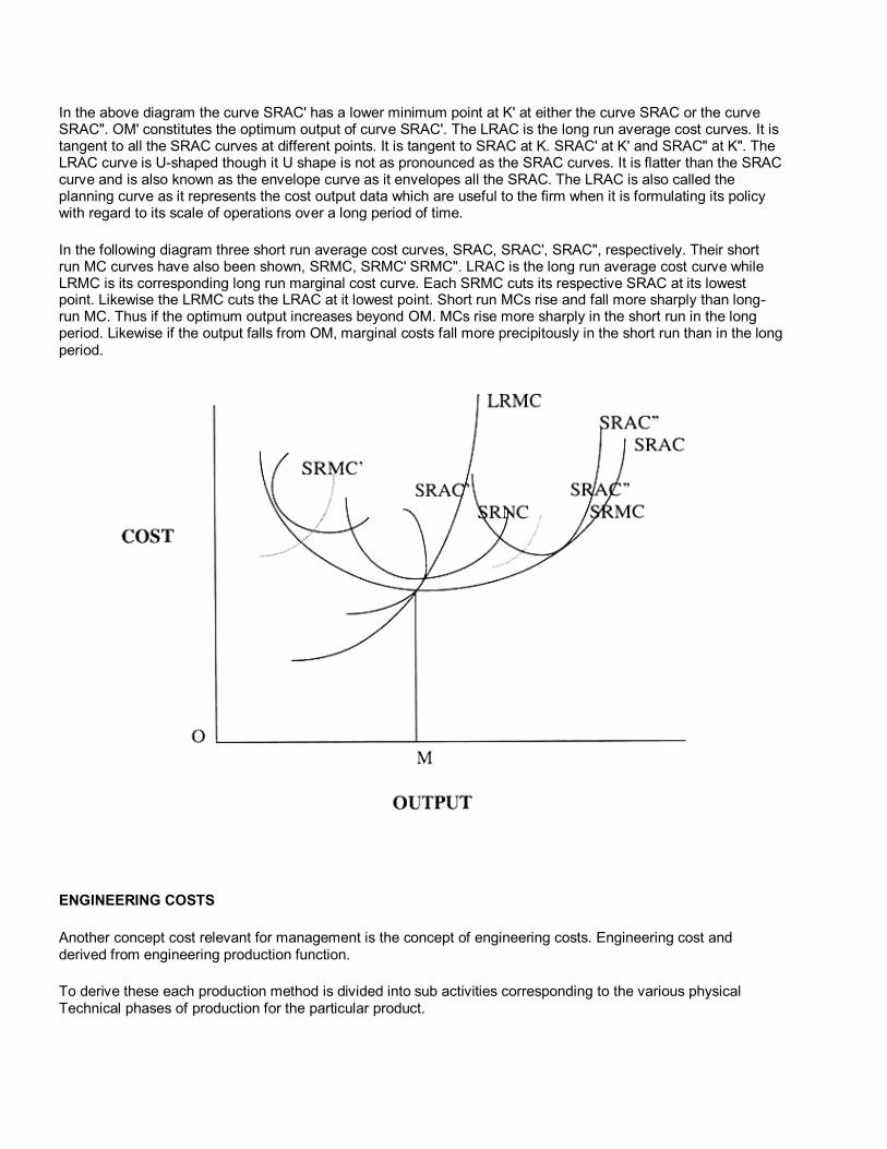
In the following diagram three short run average cost curves, SRAC, SRAC', SRAC", respectively. Their short run MC curves have also been shown, SRMC, SRMC' SRMC". LRAC is the long run average cost curve while LRMC is its corresponding long run marginal cost curve. Each SRMC cuts its respective SRAC at its lowest point. Likewise the LRMC cuts the LRAC at it lowest point. Short run MCs rise and fall more sharply than long-run MC. Thus if the optimum output increases beyond OM. MCs rise more sharply in the short run in the long period. Likewise if the output falls from OM, marginal costs fall more precipitously in the short run than in the long period.

ENGINEERING COSTS

Another concept cost relevant for management is the concept of engineering costs. Engineering cost and derived from engineering production function.

To derive these each production method is divided into sub activities corresponding to the various physical Technical phases of production for the particular product.

For each phase the quantities of factor of production are estimated and finally the cost of each phase is calculated on the basic of prevailing factor prices. The total cost of the particular method of production is the sum of cost of its different phases.

A firm has to do calculation for all available plant sizes. Production isoquants are subsequently estimated and from them, given the factor prices, the long run and short run function may be derived.

It is pertinent to note that the engineering production function and the cost functions derived from them refer usually to the production costs and do not, the administrative cost for the operation of any given plant.

ECONOMIES OF SCALE:

A firm is said to be reaping economies of scale when its LTC increases less than proportionately with increase in its scale of operations or when its LAC falls as its output expands. Alternatively it could be defined in terms of output elasticity of total cost (e TC, Q):

ETC, Q = [d (TC) / dQ]

If eTC, Q < 1 there are economies of scale. The reasons for firms to enjoy economies of scale are :

1. Due to large plant 2. Due to large firm

DUE TO LARGE FIRM: The various economies of scale which are enjoyed by the firm due to its large size are :

Specialization: This improves productivity by need for limited training for a specialized job only, learning by doing, saving of time which otherwise gets lost in moving from one activity to another. The bigger plants are able to introduce the desired level of specialization which the small firms are not able to afford.

Indivisibility: There are certain plants and equipment's which are indivisible in small size and units like tractor and tube-well for agriculture, large plants and machines for manufacturing, computers for computation work etc. Small firm's are not able to enjoy fruits of up-to date technology.

Productivity / Purchase prices: It is believed that why the productive capacity of capital equipment rises much faster than its purchase price.

Equipment Maintenance: Large plants need to carry relatively less spare parts and personnel for attending to random breakdown than small firms need to do. Thus larger firms need to produce less on repairs and maintenance, and thereby reap the economies of mass scale production.

DUE TO LARGE PLANT: There are several economies which rise to the firm due to size of the plant. It is believe that while manufacturing work is handled by individual plants, purchases of raw materials, selling of products, advertisements, fund raising and overall management are centralized at firm level.

Quantity Discounts: Firms that purchase large quantities of goods and services from suppliers are often able to negotiate large discounts which results in lower average costs in relation to small firms. Also per unit voucher cost is less for large firms vis-a-vis small firms.

Fund raising: The administrative cost of negotiating debt and floating cost of equity capital and debentures per unit of funds raised vary inversely with the size of the debt / capital ratio. In addition the securities of the large

firms are less risky than the securities of the small firm, and thereby the large firms get an edge over the small firms in fund raising.

Sales Promotion: Large firms are even able to secure quantity discounts even in securing space in various advertising media. Besides advertising outlay is like a fixed cost and so they create lesser burden per unit of unit of output rather than on smaller ones.

Innovation: Large firm's are in a better position to carry out research and development activities and thereby adopt the latest method of material procurements, production and sales, than their smaller counterparts.

Management: Large firm's enjoy the benefit of top caliber management personnel, specialization and so on.

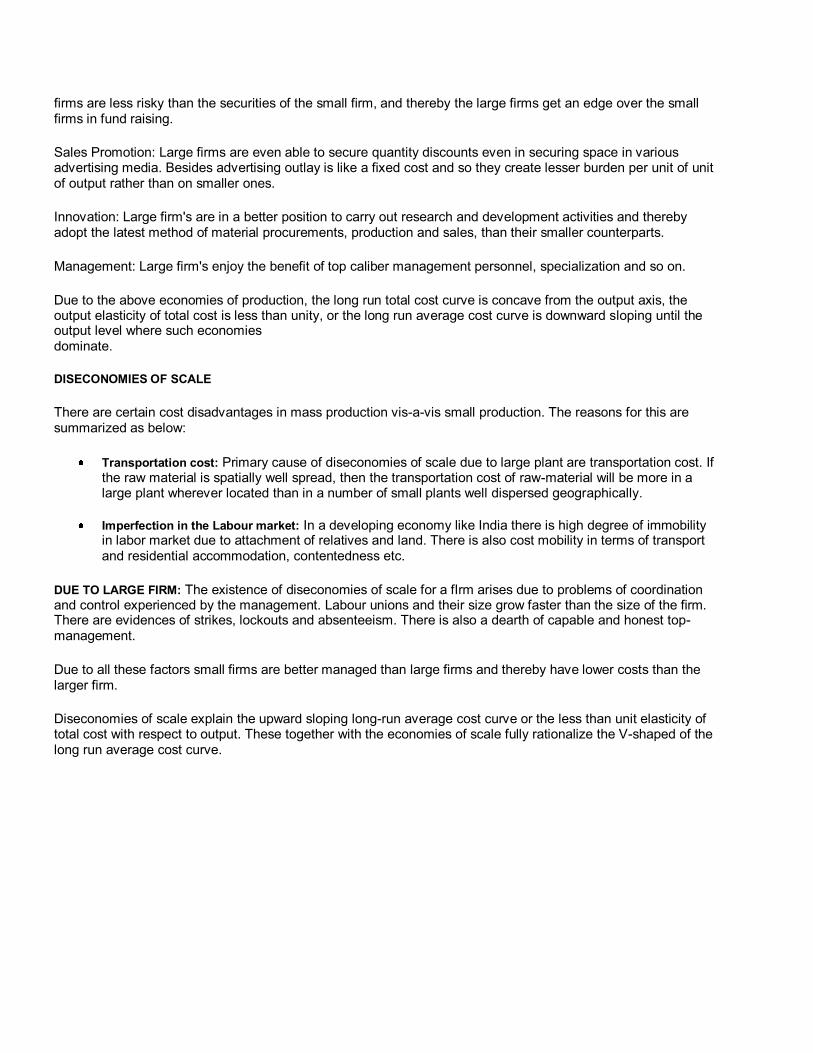
Due to the above economies of production, the long run total cost curve is concave from the output axis, the output elasticity of total cost is less than unity, or the long run average cost curve is downward sloping until the output level where such economies dominate.

DISECONOMIES OF SCALE

There are certain cost disadvantages in mass production vis-a-vis small production. The reasons for this are summarized as below:

Transportation cost: Primary cause of diseconomies of scale due to large plant are transportation cost. If the raw material is spatially well spread, then the transportation cost of raw-material will be more in a large plant wherever located than in a number of small plants well dispersed geographically.

Imperfection in the Labour market: In a developing economy like India there is high degree of immobility in labor market due to attachment of relatives and land. There is also cost mobility in terms of transport and residential accommodation, contentedness etc.

DUE TO LARGE FIRM: The existence of diseconomies of scale for a fIrm arises due to problems of coordination and control experienced by the management. Labour unions and their size grow faster than the size of the firm. There are evidences of strikes, lockouts and absenteeism. There is also a dearth of capable and honest top-management.

Due to all these factors small firms are better managed than large firms and thereby have lower costs than the larger firm.

Diseconomies of scale explain the upward sloping long-run average cost curve or the less than unit elasticity of total cost with respect to output. These together with the economies of scale fully rationalize the V-shaped of the long run average cost curve.

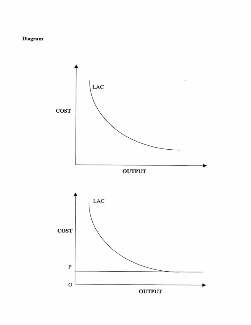
In the above figure, LAC declines as output expands up-to Q1, beyond which it stays constant at OP. The output level where LAC is the least is called the optimum level of output from the supply side. In the case of the other figure, the optimum level thus comprises of output level Q1 or any level greater than that. To distinguish Q1 output from other optimum output levels under such a situation, MES terminology can be used. The MES is the Minimum Efficient Scale and is Q1 marks the MES while output > = Q1 gives the optimum level of output.

In the second diagram LAC falls monotonically as the output expands, that is economies of scale out weight the

diseconomies of scale at all levels of output.

A business firm charters its business operations with reference to specified objective function. Its business operations are conducted in such a manner that its objective function is maximized. If objective is to maximize profits, then business operation are carried out in such a way that profits is maximized. The objectives may be sales maximization.

We shall discuss from models of the objectives of a business firm :

1. Model of project maximization 2. Baumol's model of sales maximization 3. Marris model managerial enterprise 4. Williansom's model of managerial discussion

1. Model of Project Maximization

A firm shall choose that level of output at which profit is maximized Project is the difference between total revenue and total cost

Mathematically

Total project function of a firm is

II= R-C

II = Profit

C = Total costs R = Total Revenue Clearly R = (f1 (X) And C = f2 (X), given the price P. x = output level The first order condition for the maximization of a function is that its firm derivative ( with respect to X ) be equal to zero. Differentiating the total profit function and equaling it to zero.

We obtain

Chapter 5: OBJECTIVE OF A BUSINESS FIRM

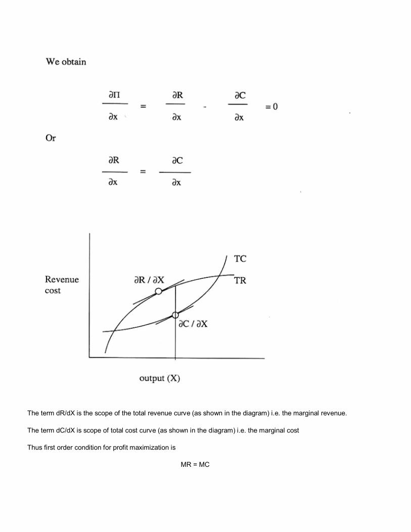
The term dR/dX is the scope of the total revenue curve (as shown in the diagram) i.e. the marginal revenue.

The term dC/dX is scope of total cost curve (as shown in the diagram) i.e. the marginal cost

Thus first order condition for profit maximization is

MR = MC

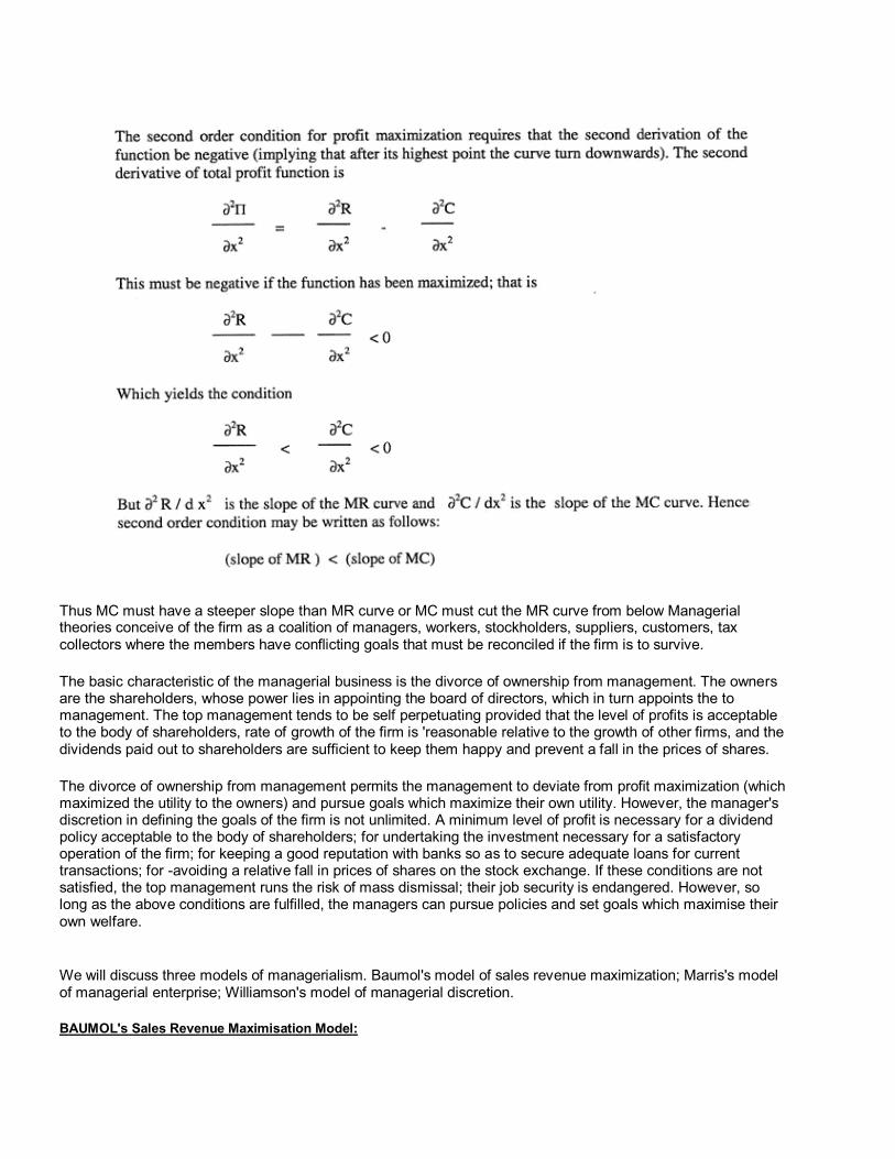
Thus MC must have a steeper slope than MR curve or MC must cut the MR curve from below Managerial theories conceive of the firm as a coalition of managers, workers, stockholders, suppliers, customers, tax collectors where the members have conflicting goals that must be reconciled if the firm is to survive.

The basic characteristic of the managerial business is the divorce of ownership from management. The owners are the shareholders, whose power lies in appointing the board of directors, which in turn appoints the to management. The top management tends to be self perpetuating provided that the level of profits is acceptable to the body of shareholders, rate of growth of the firm is 'reasonable relative to the growth of other firms, and the dividends paid out to shareholders are sufficient to keep them happy and prevent a fall in the prices of shares.

The divorce of ownership from management permits the management to deviate from profit maximization (which maximized the utility to the owners) and pursue goals which maximize their own utility. However, the manager's discretion in defining the goals of the firm is not unlimited. A minimum level of profit is necessary for a dividend policy acceptable to the body of shareholders; for undertaking the investment necessary for a satisfactory operation of the firm; for keeping a good reputation with banks so as to secure adequate loans for current transactions; for -avoiding a relative fall in prices of shares on the stock exchange. If these conditions are not satisfied, the top management runs the risk of mass dismissal; their job security is endangered. However, so long as the above conditions are fulfilled, the managers can pursue policies and set goals which maximise their own welfare.

We will discuss three models of managerialism. Baumol's model of sales revenue maximization; Marris's model of managerial enterprise; Williamson's model of managerial discretion.

BAUMOL's Sales Revenue Maximisation Model:

Baumol proposed two types of model - static & dynamic. Baumol put forward a number of justifications for the sales revenue maximization objective as opposed to profit maximization. The more important ones are:

Management Priorities -Managers are more likely to be concerned with utility maximisation on their part than

profit maximisation on the organizations part.

Management Rewards -salary increases and slack earnings (all perquisites & payments made to management in addition to salary payments) are more likely to be related to the level of sales earned by the organization than to the level of profit.

Financial Institutions -Investors are more likely top be concerned with the level and trend in sales than in the level of profit. Thus, a clear upward trend in sales will look more promising than dip in profits, where they have been used internally to finance growth.

Human Relations -It is easier to maintain a good relationship with employees when the organization has rising

levels of sales and general feeling of buoyancy.

Shareholders -The imposition of a minimum profit constraint on management by shareholders ensures that their concerns are met, while it would be more difficult to set and measure a maximum requirement.

Stability -Increasing levels of sales are usually associated with increasing market share. Therefore, the

organization may be considered to be improving its position in the market if its share is increasing.

The sales revenue maximisation model proposed was based on the assumption that the organization is operating in an oligopolistic market structure (i.e. where there are only a few sellers in the market). In this respect, certain characteristics are identifiable about the internal and external processes involved for organizations within such markets.

Baumol recognises that, since it is large organization that are most likely to be competitors within an oligopoly, then the chains of control and decision making are likely to be elongated. It is therefore considered more likely that it will take more longer to arrive at and implement decisions within such organizations than within smaller competitors.

Within, the market it is claimed that there is tacit collusion between organizations to maintain their status quo. These incumbents, once the oligopoly has settled down into an equilibrium position, are able to enjoy a quiet life and split the profits between them. Additionally, there may be a general lack of interest on the part of the organizations to compete n the market unless actions are undertaken by others to upset the current situation.

The oligopoly situation outlined above is assumed to operate in the static and dynamic models of sales revenue maximisation outlined by Baumol. The Static Model: There are number of assumptions associated specifically with the static model. These are

1. Time horizon of the firm is fixed only for a single period. There is therefore interaction with other organizations or competition.

2. During this period firm attempt to maximize sales revenue and not physical volume of output. Subsequent periods and their effect are not taken into consideration.

3. The minimum profit constraint is exogenously determined by demand of external elements like shareholders expectations banks and financial institutions. The firm thus, should always realize minimum

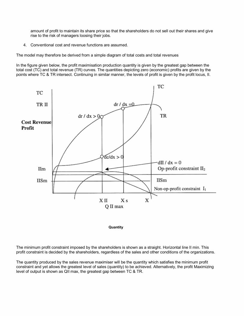
amount of profit to maintain its share price so that the shareholders do not sell out their shares and give rise to the risk of managers loosing their jobs.

4. Conventional cost and revenue functions are assumed.

The model may therefore be derived from a simple diagram of total costs and total revenues

In the figure given below, the profit maximisation production quantity is given by the greatest gap between the total cost (TC) and total revenue (TR) curves. The quantities depicting zero (economic) profits are given by the points where TC & TR intersect. Continuing in similar manner, the levels of profit is given by the profit locus, II.

Quantity

The minimum profit constraint imposed by the shareholders is shown as a straight. Horizontal line II min. This profit constraint is decided by the shareholders, regardless of the sales and other conditions of the organizations.

The quantity produced by the sales revenue maximiser will be the quantity which satisfies the minimum profit constraint and yet allows the greatest level of sales (quantity) to be achieved. Alternatively, the profit Maximizing level of output is shown as QII max, the greatest gap between TC & TR.

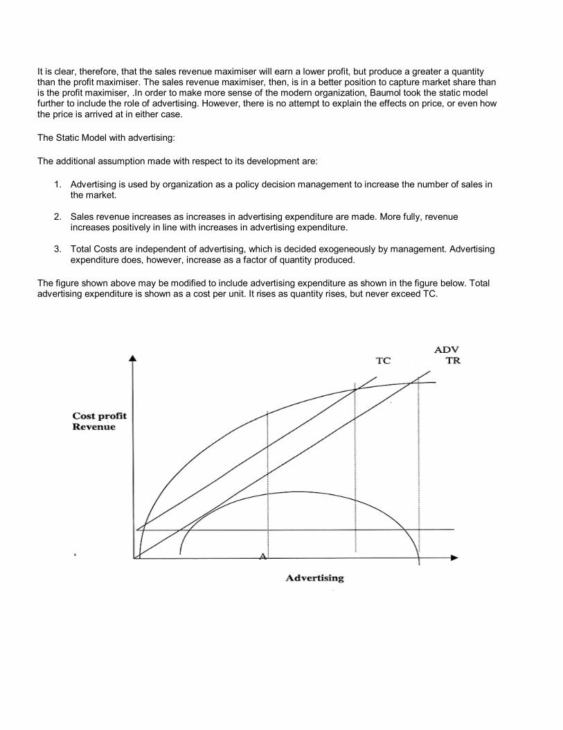
It is clear, therefore, that the sales revenue maximiser will earn a lower profit, but produce a greater a quantity than the profit maximiser. The sales revenue maximiser, then, is in a better position to capture market share than is the profit maximiser, .In order to make more sense of the modern organization, Baumol took the static model further to include the role of advertising. However, there is no attempt to explain the effects on price, or even how the price is arrived at in either case.

The Static Model with advertising:

The additional assumption made with respect to its development are:

1. Advertising is used by organization as a policy decision management to increase the number of sales in the market.

2. Sales revenue increases as increases in advertising expenditure are made. More fully, revenue increases positively in line with increases in advertising expenditure.

3. Total Costs are independent of advertising, which is decided exogeneously by management. Advertising expenditure does, however, increase as a factor of quantity produced.

The figure shown above may be modified to include advertising expenditure as shown in the figure below. Total advertising expenditure is shown as a cost per unit. It rises as quantity rises, but never exceed TC.

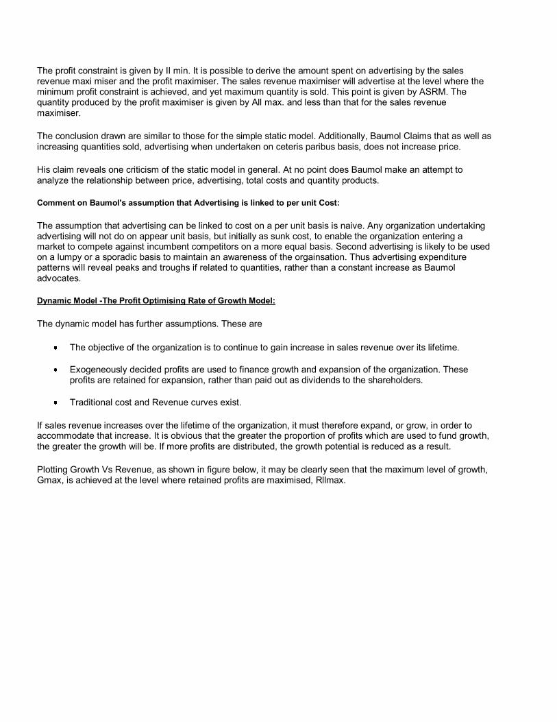
The profit constraint is given by II min. It is possible to derive the amount spent on advertising by the sales revenue maxi miser and the profit maximiser. The sales revenue maximiser will advertise at the level where the minimum profit constraint is achieved, and yet maximum quantity is sold. This point is given by ASRM. The quantity produced by the profit maximiser is given by All max. and less than that for the sales revenue maximiser.

The conclusion drawn are similar to those for the simple static model. Additionally, Baumol Claims that as well as increasing quantities sold, advertising when undertaken on ceteris paribus basis, does not increase price.

His claim reveals one criticism of the static model in general. At no point does Baumol make an attempt to analyze the relationship between price, advertising, total costs and quantity products.

Comment on Baumol's assumption that Advertising is linked to per unit Cost:

The assumption that advertising can be linked to cost on a per unit basis is naive. Any organization undertaking advertising will not do on appear unit basis, but initially as sunk cost, to enable the organization entering a market to compete against incumbent competitors on a more equal basis. Second advertising is likely to be used on a lumpy or a sporadic basis to maintain an awareness of the orgainsation. Thus advertising expenditure patterns will reveal peaks and troughs if related to quantities, rather than a constant increase as Baumol advocates.

Dynamic Model -The Profit Optimising Rate of Growth Model:

The dynamic model has further assumptions. These are

The objective of the organization is to continue to gain increase in sales revenue over its lifetime.

Exogeneously decided profits are used to finance growth and expansion of the organization. These profits are retained for expansion, rather than paid out as dividends to the shareholders.

Traditional cost and Revenue curves exist.

If sales revenue increases over the lifetime of the organization, it must therefore expand, or grow, in order to accommodate that increase. It is obvious that the greater the proportion of profits which are used to fund growth, the greater the growth will be. If more profits are distributed, the growth potential is reduced as a result.

Plotting Growth Vs Revenue, as shown in figure below, it may be clearly seen that the maximum level of growth, Gmax, is achieved at the level where retained profits are maximised, Rllmax.

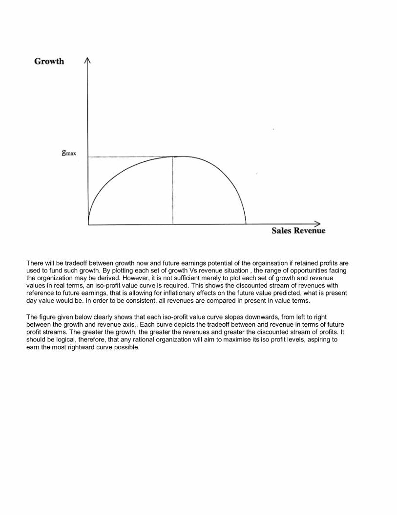
There will be tradeoff between growth now and future earnings potential of the orgainsation if retained profits are used to fund such growth. By plotting each set of growth Vs revenue situation , the range of opportunities facing the organization may be derived. However, it is not sufficient merely to plot each set of growth and revenue values in real terms, an iso-profit value curve is required. This shows the discounted stream of revenues with reference to future earnings, that is allowing for inflationary effects on the future value predicted, what is present day value would be. In order to be consistent, all revenues are compared in present in value terms.

The figure given below clearly shows that each iso-profit value curve slopes downwards, from left to right between the growth and revenue axis,. Each curve depicts the tradeoff between and revenue in terms of future profit streams. The greater the growth, the greater the revenues and greater the discounted stream of profits. It should be logical, therefore, that any rational organization will aim to maximise its iso profit levels, aspiring to earn the most rightward curve possible.

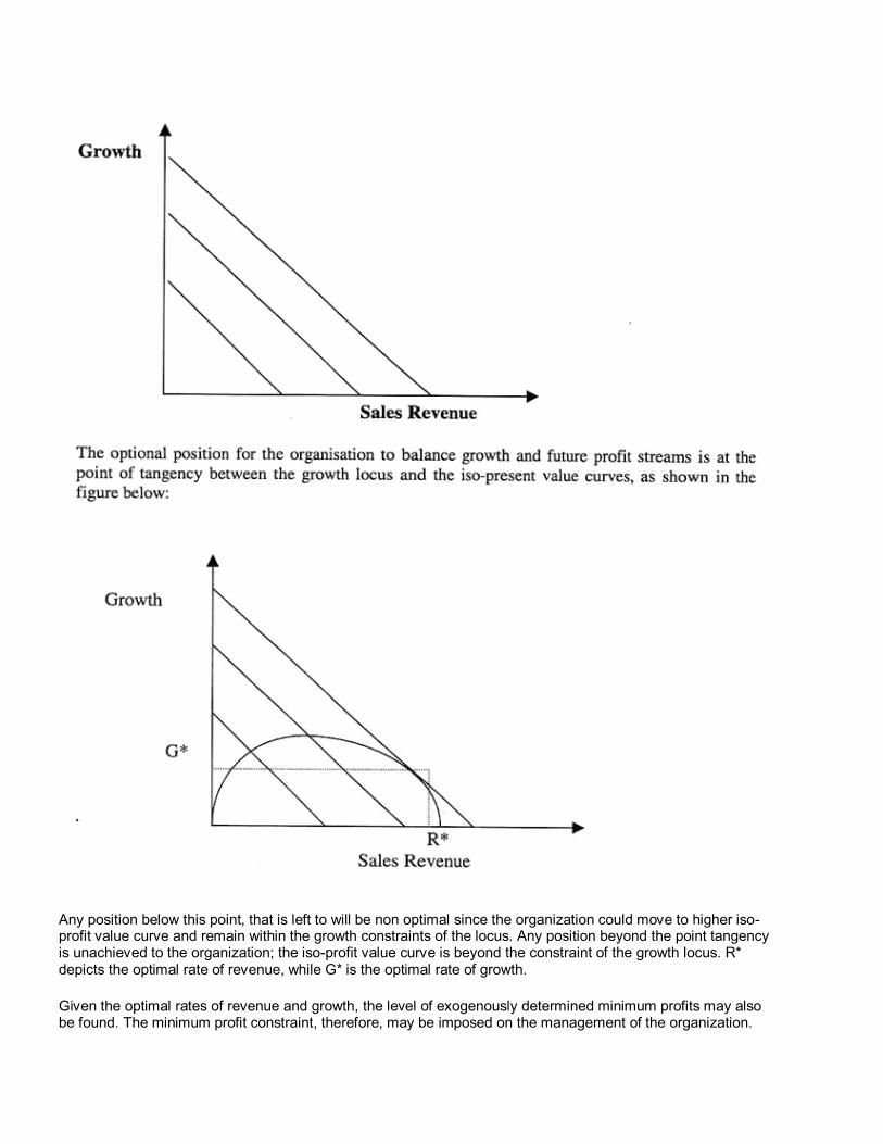
Any position below this point, that is left to will be non optimal since the organization could move to higher iso-profit value curve and remain within the growth constraints of the locus. Any position beyond the point tangency is unachieved to the organization; the iso-profit value curve is beyond the constraint of the growth locus. R* depicts the optimal rate of revenue, while G* is the optimal rate of growth.

Given the optimal rates of revenue and growth, the level of exogenously determined minimum profits may also be found. The minimum profit constraint, therefore, may be imposed on the management of the organization.

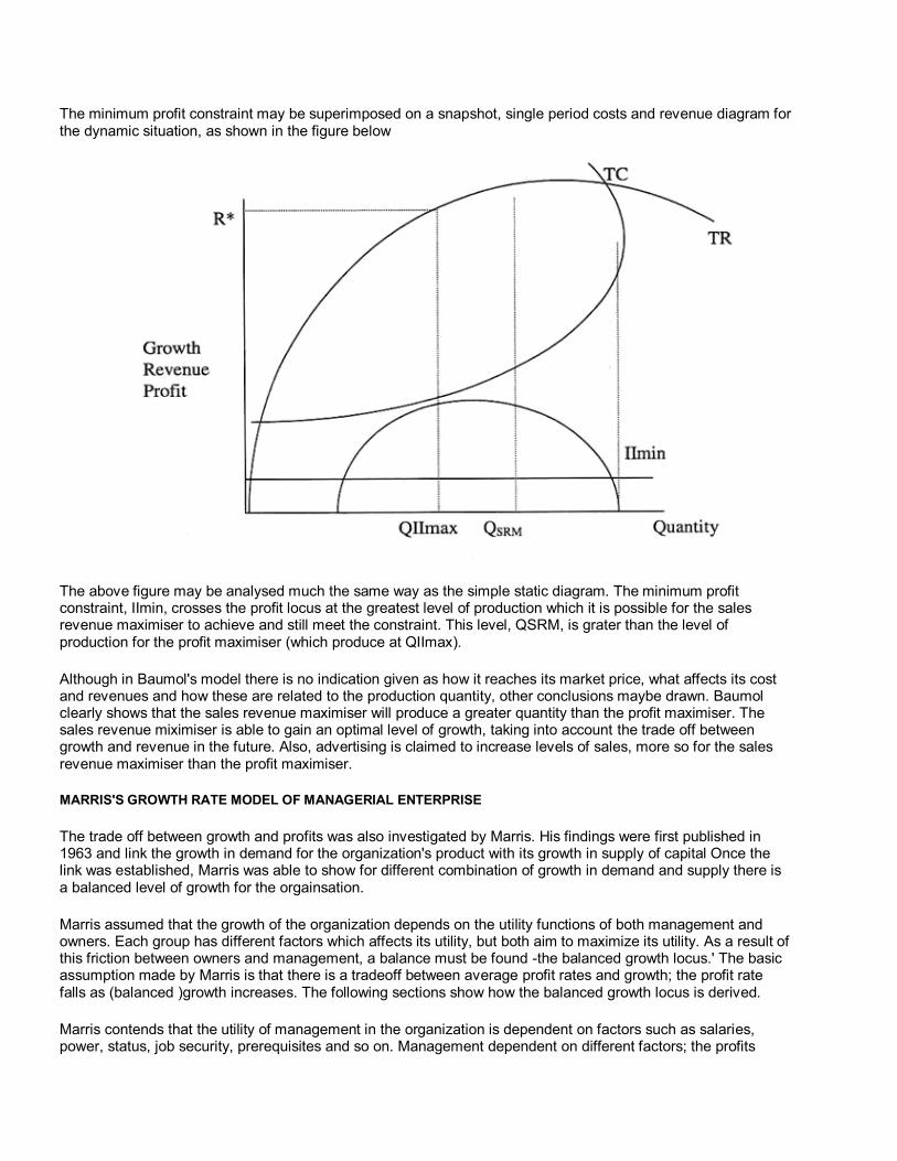
The minimum profit constraint may be superimposed on a snapshot, single period costs and revenue diagram for the dynamic situation, as shown in the figure below

The above figure may be analysed much the same way as the simple static diagram. The minimum profit constraint, IImin, crosses the profit locus at the greatest level of production which it is possible for the sales revenue maximiser to achieve and still meet the constraint. This level, QSRM, is grater than the level of production for the profit maximiser (which produce at QIImax).

Although in Baumol's model there is no indication given as how it reaches its market price, what affects its cost and revenues and how these are related to the production quantity, other conclusions maybe drawn. Baumol clearly shows that the sales revenue maximiser will produce a greater quantity than the profit maximiser. The sales revenue miximiser is able to gain an optimal level of growth, taking into account the trade off between growth and revenue in the future. Also, advertising is claimed to increase levels of sales, more so for the sales revenue maximiser than the profit maximiser.

MARRIS'S GROWTH RATE MODEL OF MANAGERIAL ENTERPRISE

The trade off between growth and profits was also investigated by Marris. His findings were first published in 1963 and link the growth in demand for the organization's product with its growth in supply of capital Once the link was established, Marris was able to show for different combination of growth in demand and supply there is a balanced level of growth for the orgainsation.

Marris assumed that the growth of the organization depends on the utility functions of both management and owners. Each group has different factors which affects its utility, but both aim to maximize its utility. As a result of this friction between owners and management, a balance must be found -the balanced growth locus.' The basic assumption made by Marris is that there is a tradeoff between average profit rates and growth; the profit rate falls as (balanced )growth increases. The following sections show how the balanced growth locus is derived.

Marris contends that the utility of management in the organization is dependent on factors such as salaries, power, status, job security, prerequisites and so on. Management dependent on different factors; the profits

earned, the quantity sold, levels of capital available to the organization, market share and the public esteem gained.

Growth in demand

Management decisions (delegated by owners) will affect the rate of growth in demand for the organization's product. On constraining factor is the tradeoff between job security and the risk relating to projects undertaken to increase demand.

Growth in demand is achieved in two ways: diversification into new products and differentiation of current products. Marris does not differentiate between the different methods. What is important however, is that the percentage of new products succeeding in the market place is negatively linked to the rate of profits earned by the organization. There is a tradeoff between funds for diversification and funds declared as profits, because funds declared as profits effectively decrease the amount of investment which may be made in research and development of new products. Investment into research and product form a cost which will obviously detract from the profits of the organization in the period in which they accrue.

Management therefore needs to make a decision between the rate of diversification and the rate of profit it desires. The decision is, however, more complex than simply balancing diversification and profits. Managerial utility is very much determined by job security. Job security may be defined in the financial terms as s combination of the following ratios and is known as the' financial security management:

Leverage = Total debt/total assets -The greater the leverage, the more the organization owes its financial backers, the more difficult it will be to borrow until the ration is reduced.

Liquidity = liquid assets / assets -The greater the liquidity, the more stock and other saleable assets and organization has in proportion to its total assets. Lower liquidity indicates a capital intensity on the pat of the organization.

Retention Ratio = retained profits / total profits -The greater the retention ratio, the more the organization is retaining for future projects. The lower the retention ratio, the higher the funds to pay dividends to shareholders.

Growth in Supply

Countering the growth in demand of the organization is the growth in supply of capital. This depends on the owners of the organization and their utility. Quite simply, the greater the level of retained profits, the lower the level of profits available for dividends. The owners must therefore decide whether to release funds for growth, or to take a cut of the success to date. The higher the rate of retained profits, the greater potential for growth the organization has.

Marris brings together the utility objectives of the owners of the organization with those of its managers. The result is a picture of the organization's possibilities for growth and diversification. This is only snapshot, however, due to decision made by the management with reference to financial security constraints and by the owners with reference to the retained profits levels. A criticism of Marris's work exists because there is an assumption that the organization is operating in a stable business environment and that decisions are made by those who implement them.

An additional criticism relates to the assumption made by Marris that research and development funds and advertising are lumped together. Obviously, product diversification cannot take place without R&D. Also, to be successful, developments usually need to be advertised. The lumping together of these is considered to be native by many commentators because R &D and advertising require different processes and skills and take place at different times.

WILLAIMSON'S MODEL OF MANAGERIAL DISCRETION

Williamson argues that managers have discretion in pursuing policies which maximise their own utility rather than attempting the maximisation of profits which maximises the utility of owner- shareholders. Profit acts as a constraint to this managerial behavior, in that the financial market and the shareholders require a minimum profit to be paid out in the form of dividends, otherwise the job security of management is endangered.

The managerial utility function includes such variables as salary, security, power, status, prestige, professional excellence. Of these variables only the first (salary) is measurable. The others are non-pecuniary and if they are to be operational they must be expressed in terms of other variables with which they are connected and which are measurable. This is attained by the concept of expense preference, which is defined as the satisfaction which managers derive from certain types of expenditures. In particular, staff expenses on emoluments, and funds available for discretionary investment give to managers a positive satisfaction because these expenditures are a source of security and reflect the power, status, prestige and professional achievement of managers.

Staff increases are to certain extent equivalent to promotion, since they increase the range of activity and control of managers over resources. Being the head of a large staff is a symbol of power, status and prestige

Manager's prestige, power and status are to a large extend reflected in the amount of emoluments or slack they receive in the form of expense accounts, luxurious offices, company cars, etc. Emoluments are economic rents accruing to the managers; they have zero productivity in that, if removed, they would not cause the managers to leave the firm and seek employment elsewhere.

They are discretionary expenditures which are made possible because of the strategic position that managers have in the running of the business.

Finally, the status and power of managers is associated with the discretion they have in undertaking investments beyond those required for the normal operation of the firm. These minimum investment requirements are included in the minimum profit constraint together with the amount of profits required for a satisfactory dividend policy.

Staff expenditures, emoluments and discretionary investment expenses are measurable in money terms and will be used as proxy-variables to replace the no-operational concepts (power, status, prestige, professional excellence) appearing in the managerial utility function. Thus the utility function of the mangers may be written in the form

U = f(S,M, 1D)

Where

S = Staff expenditure, including managerial salaries.

M = Managerial emoluments

1D = Discretionary investments

WEAKNESS OF MANAGERIAL MODELS

There are a number of generic criticisms which may be made of the managerial theories of the firm. The managerial models are considered to be naive in reference to their coverage of organizational behavior within

competitive markets such as oligopoly. Additionally, they offer no consideration of research and development activities which many organizations undertake as a matter of course. The main criticisms are:

Profit is considered to be 'given', that is, exogenous to the model; this is particularly true of the minimum profit constraint included in many cases. Therefore there is no consideration of the manner in which desirable profit levels are obtained or decided on.

It is assumed that profits are used to fund growth. There is no consideration of alternative ways in which growth may be funded, such as share issues or borrowing from financial institutions. However,' Marris does consider the balance between internal and external finances in his work.

Prices are assumed to be constant and organizations are assumed to be operating within stable oligopoly environments.

Quantities produced are related to revenues of the organization, not to advertising or other factors.

Research and development and product line extensions are ignored, except in the case of Marris model which does include within the average profit marginal acknowledgement of product differentiation. Implicitly, this must include research and development.

Finally, it should be noted that the managerial models give insight into only a snapshot of the organization's

position. There is no explanation or outline of what future situations may be like. Therefore, the model provide

only a one-off explanation of what organization may look like and +the manner in which they may act.

Chapter 6: PRICING METHODS

Managerial decision making consists of a number of procedures at each individual stage of the product manufacturing. They are related to the product development depending on the market requirement, product manufacturing, product distribution and marketing of the same to realize the company's sales targets.

One of the important factors which assist the company in realizing its profits through targeted sales is the Pricing Policy, it formulates. As a result the method of the company's Pricing Policy plays an important role in the Managerial decision making.

Price, in fact, is the source of revenue which the firm seeks to maximise. Also it is the most important device a firm can use to expand its clientele base. The company should fix the price reasonably because if the price is set too high, it may lead it to loose its market share. On the other hand, if the price is set too low the company may not recover its cost. so the right choice of the Price fixation would depend on number of factors and wide variety of conditions prevailing in the market. Moreover the pricing decisions have to be reviewed and formulated from time to time.

Some of the factors which affect the choice of the pricing policies are:

1. Business Objectives: This relates to rate of growth, establishing and increasing its market share and maintenance of control and finally profit realisation. All these concepts play an important role in pricing policy formulation.

2. Competition level: It is important for a company to offer the product which satisfy the wants and desires of the consumer than the one which sells at the lowest price.

3. 4P's: Pricing happens to be one of the core concepts of marketing but a firm must consider it together with Product, Place & Promotion.

4. Price sensitivity: Factors like variability in the consumer behavior consumer income level, marketing effect, nature of product and after sales service among others effect the price sensitivity.

5. Available information: The demand supply gap goes a long way in affecting the choice of the pricing policy determination for as company.

Pricing hence is more a matter of judgment since every pricing situation is different from each other and as such there is no formula existing for the price fixation.

Objectives of Pricing Policies

Pricing policies form an integral part of the company's overall business strategy. Some of the important objectives, which the company should take into consideration, are:

1. Profit maximisation for the company's products 2. Relation of long term goals of the company. 3. Successfully thwart the competitors. 4. Flexibility in pricing to meet the changes in the market. 5. Achieving a satisfactory rate of return

Factors affecting Pricing Policies

The company should determine its pricing policies in such a way that depending on the market trends, the company is able to adapt itself to the changes occurring in the market.

Few of the factors are enlisted below:

1. Cost involved 2. Demand elasticity 3. Consumer psychology 4. Price changes

o Reduction in prices o Increase in Prices

5. Type of product 6. Competitors in the market 7. Product segmentation and positioning. 8. Market structure and promotional policies 9. Degree of integration 10. Business Expansion 11. Complementary and substitution products and 12. Other considerations

o Individual o Firm's o Economic

PRICE FORECASTING

A Business unit is constantly faced with the risk of a substantial change in the prices of raw materials as 'well as its products, these changes may be a part of general economic fluctuations but, at times the prices may change during the period of economic stability also

The first step towards successful price forecasting is the understanding of nature of the commodity and its market. We should have the knowledge of the demand -supply conditions, i.e.

1. Demand elasticity: Where the demand is elastic; a given change in supply will bring a less sever change in price than where the demand is inelastic.

2. Change in supply of commodity: When the change in demand for commodity takes place price change will depend on the supply conditions, which in turn will depend on the conditions of production e.g. supply manufactured product can be altered according to the demand condition. The price tends to vary for that product where the supply of a product cannot be in accordance with that of demand.

3. Influence of supply and demand on the price: There are many products particularly agricultural, whose demands remains constant but where the supply may change continuously. So that analysis should be made from the supply side and for the manufactured product the rapid demand change can be matched with the supply adjustments.

4. Related Commodities: The prices of many manufactured goods depends on prices of raw material particularly on the current prices. The manufacturer while pricing the product will take only this pricing into consideration.

5. Type of product: The price of commodity will depend on the other one specially if it is a by product. In that case supply of that by product will depend on the main product and not on its (By-product's) demand conditions.

6. Supply - Controllable and predictable: It may be possible for the supply of a commodity to change substantially but this change may be unpredictable and beyond control e.g. an increase in the supply of crude oil will depend on the oil striking capacity.

7. Competitive situations: In case where a dominant producer leads the market, his probable price policy becomes a significant factor in making the price forecast. In case of a severe price competition, resorting to the price cutting would be frequent and uncertain, specially in the buyer's market.

Prospective supply and demand

In price forecasting a knowledge about the prospective supply and demand conditions is also essential. In fact, besides estimating the supply and demand conditions prevailing at the time of the forecast it is imperative to find the probable demand and supply conditions during the next six months.

Prospective Supply

The current value of production of commodity should be compared with the total productive capacity in order to ascertain the extent of excessive productive capacity in the market. An excess of capacity creates a persistent tendency towards over production and acts as a restraint upon a rise in the price.

The existing cost -Price relationship may also determine the prospective supply. There will be a tendency among the firms producing a commodity to curtail the production if price decreases over the cost of production. On the other hand, when the price exceeds the variable cost they would enter the industry once again.

Prospective Demand

The prospective demand is determined by the nature of need for the need of that commodity and the willingness of the buyer to buy the commodity and their purchasing power.

Relational price changes

An analysis of a price movement of a commodity over a period of time will reveal certain fluctuation. These fluctuations and their relationships are helpful in price forecasting.

Some of the fluctuations observed are:

1. Seasonal price variation: These are common in case of number of commodities notably agricultural and food products such variations would take place in markets having seasonal cycles. These variations may take place due to seasonal fluctuation in the price of raw materials also.

2. Cyclical price variation: During the business cycle, price of all commodities would generally record fluctuations. So it becomes essential to realize this effect on the commodities in different ways. The general business conditions influence the commodity prices through changes in the demand supply relationships in the market for each individual commodity.

3. Cob -Web Cycle: These cycles occur on account of the cumulative effect of the price expectations of the millions of independent producers. When farmers expect higher prices in future, they plan independently to producer more. Also new ones enter the field. As a result, the aggregate output, when the future date arrives, is so large that the price falls. When the prices fall, all the producers plan to produce less, once they have suffered losses on the account of non-materialization of their expected prices. This time the cumulative effect of smaller output plan leads to the shortage of products which in turn increases the prices.

PRICING METHODS

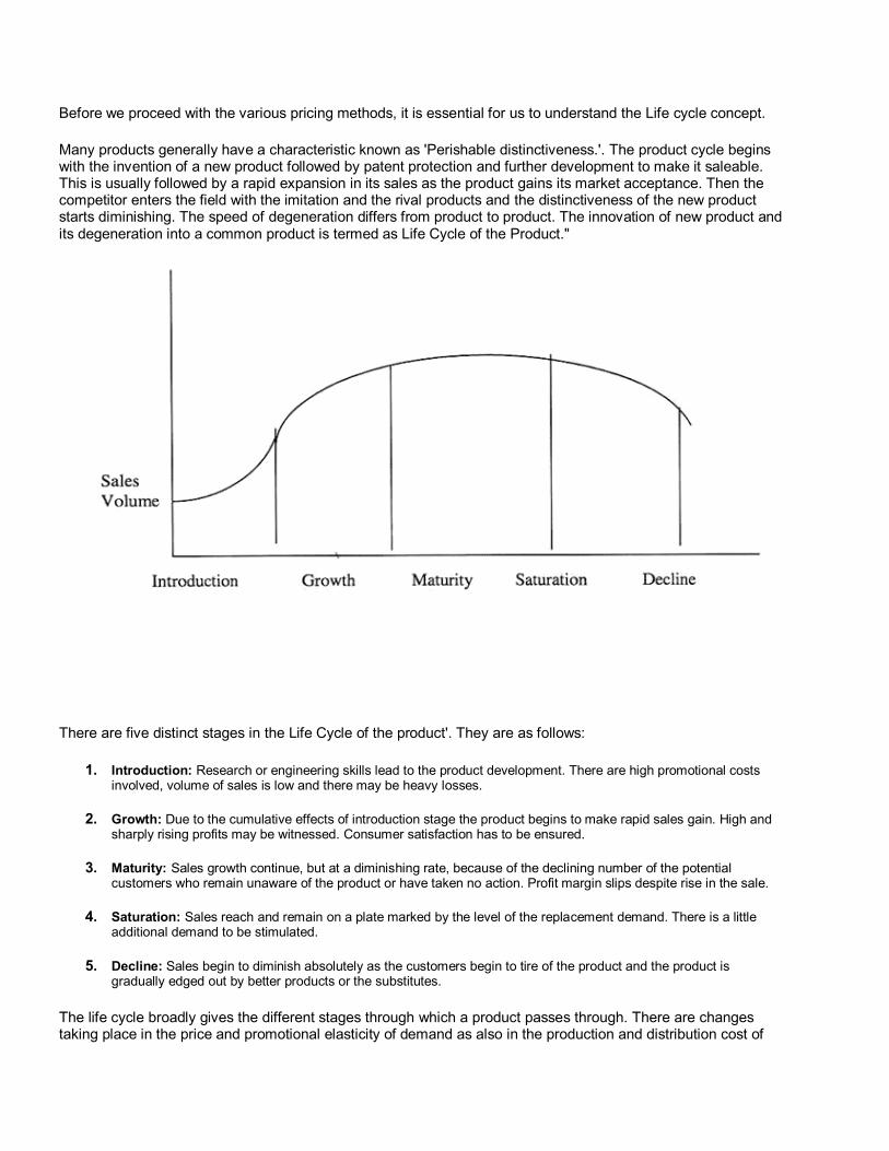
Before we proceed with the various pricing methods, it is essential for us to understand the Life cycle concept.

Many products generally have a characteristic known as 'Perishable distinctiveness.'. The product cycle begins with the invention of a new product followed by patent protection and further development to make it saleable. This is usually followed by a rapid expansion in its sales as the product gains its market acceptance. Then the competitor enters the field with the imitation and the rival products and the distinctiveness of the new product starts diminishing. The speed of degeneration differs from product to product. The innovation of new product and its degeneration into a common product is termed as Life Cycle of the Product."

There are five distinct stages in the Life Cycle of the product'. They are as follows:

1. Introduction: Research or engineering skills lead to the product development. There are high promotional costs involved, volume of sales is low and there may be heavy losses.

2. Growth: Due to the cumulative effects of introduction stage the product begins to make rapid sales gain. High and sharply rising profits may be witnessed. Consumer satisfaction has to be ensured.

3. Maturity: Sales growth continue, but at a diminishing rate, because of the declining number of the potential customers who remain unaware of the product or have taken no action. Profit margin slips despite rise in the sale.

4. Saturation: Sales reach and remain on a plate marked by the level of the replacement demand. There is a little additional demand to be stimulated.

5. Decline: Sales begin to diminish absolutely as the customers begin to tire of the product and the product is gradually edged out by better products or the substitutes.

The life cycle broadly gives the different stages through which a product passes through. There are changes taking place in the price and promotional elasticity of demand as also in the production and distribution cost of

the product. Pricing Policy, therefore, must be properly adjusted over the various phases of the life cycle of the product.

The various Pricing methods are:

Cost Plus or Full Cost method pricing,

Rate of Return pricing,

Marginal cost pricing,

Going rate pricing,

Team pricing,

Mark-up and Mark-down pricing,

Value pricing,

Position based pricing,

Exports pricing,

Dual pricing

Administered pricing,

Skimming pricing,

Penetration pricing,

Peak load priding,

Charm pricing,

Discrimination pricing.,

Product mix pricing.

Cost-plus or full-cost pricing:

This is the most common method used for pricing. Under this method, the price is set to cover the costs (materials, labour and overhead) and a predetermined percentage for profit. The percentage differs from industry to industry. This may reflect differences in competitive intensity, differences in cost base, differences in rate of turnover and risk.

Ordinarily the profits are kept at a margin sensitive to the market conditions. Mark-ups may be determined by trade associations either by the means of advisory price-list or by actual list of mark ups distributed to members. Usually profit margins under price control are so set as to make it possible for even the least efficient firms to survive. This method ignores the demands -there is no necessary relationship between the costs and what the people pay for the product. Also it fails to reflect the forces of the competition adequately.

Example

All the stationery products are priced in this way.

Rate of Return pricing

It is a refined variant of full cost pricing. Under this method a firm starts with a rate of return they consider satisfactory and then set a price that allows them to earn that return when there plant utilization is at some standard rat. In other words the company determines the standard cost at standard volume and add the margins necessary to return a target rate of profit over the long run.

This can be broadly grouped under the following:

1. Fixing prices to maintain constant percentage mark up over the cost,

2. Fixing prices to maintain the profit as constant percentage of sale, and

3. Fixing prices to maintain a constant return on the investment capital.

Example

Most products are priced I this way for instance Philips audio systems are currently priced based on what the manufacturers estimate the returns to be.

Marginal cost pricing

Both under the full cost pricing and rate of return pricing, the prices are based on total cost comprising fixed and variable cost. Under marginal cost pricing, the fixed costs are ignored and prices determined on the basis of marginal cost. The firm uses only those costs that are directly attributable to the output of a specific product.

With marginal cost pricing, the firm seeks to fix its prices so as to maximise its total contribution to fixed cost and profit. Unless the manufacturer's products are in direct competition with each other, this objective is achieved by considering each product in isolation and fixing its price at a level which is calculated to maximise its total contribution.

With marginal cost pricing, the prices are never rendered up-competitively because of a higher fixed cost are higher than those of the competitor. The firm's prices will be rendered un- competitive by high variable cost, and these are controllable in short run

Marginal cost more accurately reflects future as distinct from present cost level and relationship. This method also helps the manufacturer to develop a far more aggressive pricing policy than the full cost pricing.

In a period of business recession, firm's using marginal cost pricing may lower prices in order retain its market share. This may lead other firms to reduce their prices leading to cut- throat competition. The price cut may be upto such an extent that the fixed cost are not covered and thus a fair return on the investment is not obtained.

Example

Nestle Tea is priced based on this method.

Going Rate Pricing

Here instead of cost, the emphasis is on the market. The firm adjusts its own price policy to general pricing structure in the industry. This may seem to be a rational pricing policy when the costs are difficult to measure. Many cases of this type are situations of price leadership. Where price leadership is well established, charging according to what competitors are charging, is the only safe policy.

It must be noted that this pricing is not quiet the same as accepting the price impersonally set by a near perfect market. Whether it would seem that the firm has some power to set its own price and could be a price maker if it chooses to face all the consequences.

Example

Since Nescafe is the market leader in the instant coffee segment, hence every manufacturer wanting to enter this segment has to toe Nescafe's line.

Team pricing

According to this method, the companies sometimes assign special roles to the various products they sell. Some items may be used as promotional items which are priced and advertised with prime purpose of attracting the customers and other may be intended to make up for the low margin obtained on the promotional items.

Example

Several retailers give free items with certain items. Pantaloon, Allen Solly & Van Heusen are examples, for instance with a Van Heusen Blazer you can choose Van Heusen tie for free.

Mark-up and Mark - down pricing

When a retailer follows the practice of fixing the price over the one at which he has obtained the product, such that it covers the cost and leaves a reasonable profit margin he is said to follow the mark-up policy.

In case certain goods are not sold within a reasonable time, the retailer pulls the price down i.e. "marks down" the product price.

Example

During Diwali as the day approaches the firecracker prices increase and on the diwali afternoon the prices are significantly marked down.

Value Pricing

In recent years, several companies have adopted value pricing by which they charge a low price for a high quality product. The company's strategy is to attract the customer by offering him a product of higher quality at an affordable price. This in turn helps the company to increase its customer base which adds to the total profitability of the business.

Example

Toyota launched its "Lexus" model wit all the features of a luxury car but at a lesser price than those in the same segment. Going by the features it was offering the company could have priced the product close to the Mercedes models but the company priced the product lesser than it. The reason behind this was that Toyota realised the fact that substantial number of customers worldwide wanted and could afford an expensive car. Within this group, there were many customers who rated Mercedes as overpriced. The company was able to cash on this concept and the success of "Lexus" model is a live example of this.

Segment based pricing

In this type of pricing method, the pricing of the product is determined by the market position for which it is targeted. The company identifies the various segments existing in the market and then prices the product accordingly. Generally, the pricing here is done such that the company position its products in between two segments of the market and tries to put in the possible features of both the segments, so that it can pull the customer from both the segments towards its product.

Example

Case of Hyundai "Santro" is one of the live examples of this pricing method. The company has launched three models starting from 2.99 lacs. Their idea is to eat into the market share of both Maruti 800 model as well as that of the Maruti "Zen" model. The company has come out with 999 cc model and they are targeting the customers from both the segments.

Offering the choice to the potential Maruti 800 customers in the form of more value in the car at a little more cost and to that of Maruti "Zen" an equally well substitute, at a cheaper price.

Export Pricing

Under this type of the pricing method, decision are based on the complete understanding of the varied market situations which differ from country to country, product to product and also from time to time. Price is the most important single consideration in the International marketing. What is more, individual exporter have no control over the price. The other important non-price factors are assured deliveries, after sales service, availability to supply in bulk and a complete range of the product. In respect of export pricing the concept of " Marginal pricing" comes in very handy. If an exporter is able to realise its marginal cost, including the additional cost incidental to export he will not suffer a loss as far as exports are concerned.

Example

In case of exports of traditional products such as handicrafts India is the major exporter and very often the prices are able to cover the total cost involved. The pricing here should be able to attract the customer overseas as that will directly affect the profitability for the exporter.

Dual Pricing

This refers to a two-part system where fixed price concept applies only to the part of the output and the remaining output is allowed to be sold at prices determined by the market forces.

It has to be recognised that demand under a dual pricing system will not be the same under single free market system. Under this system, a link is introduced in the demand and supply is made at fixed price the main advantage of dual pricing is that it seeks to protect the vulnerable sections of the society for the balance amount.

Example

In a sugar industry for example it is not likely that at the existing level of sugar in an absolutely free market would be say Rs.700 per quintal (which is the average price realised by the a sugar factory at a levy price of Rs. 450 for 65% of output at after market price of Rs.900 for 35% of output) Sugar also would not reach the same group as under a free market system. Assuming that I a free market, a price of Rs.800 were to be reached, a large number of people who obtain sugar at the controlled price, would not be able to obtain sugar under the free market price.

Administered pricing policy

As the name suggests, in this type of pricing the price of the product is determined and controlled, entirely by the Government. The market forces prevailing in this case do not affect the prices.

The objectives of this method are to maintain the prices of essential commodities and also of the essential inputs to avoid triggering of price escalation and also to ensure the economic prices to the uneconomic unit.

Example

The price of Steel is controlled and maintained by the Government. We have players like Steel Authority of India Limited (A public sector undertaking), Tata Iron and Steel Company (Private Sector) and Essar Steel (Again a private sector). Since steel happens to be an important raw material for most of the manufacturing companies. The prices are govt. controlled to avoid any price manipulations.

Skimming

In this pricing method the innovator can set a high price for a while and "milk" the customers who are willing to pay that high price. Then, after he has made sales to these prime customers and after the competitors have come into the industry due to high margin of the profit, he reduces the price of his product.

Since high prices are unlikely to scare away the pioneer customers, the demand is likely to be price inelastic in early stages than later. Also with the help of such a policy the producer can divide total market into various segments based on respective elasticity of demand.

Example

Polaroid was able to skim the market when its cameras were introduced for the first time on their novelty value, since no competitor had no similar product.

Penetration

Under this pricing method, the innovator sets a lower price to start with. The underline of this strategy is to widen the market as the start by getting more customer acquainted with the product. The widened market and consequently the mass production of the product, it is expected, will reduce the cost of production.

Such a policy is useful in short period where the price elasticity is high and where the cost of production reduces sharply as a result of increase in production. Generally, a low penetration price policy is adopted to ward off the possibility of potential entry of new competitor.

Example

Compaq to introduce itself in the branded computer market introduced the de Deskpro 1000 series at a lower price than its other top line models such as the Deskpro 2000. Similarly Kwality Walls introduce its icecrearns at a price even lower that all prevailing firms.

Pack Load

There are certain products which are non-storable and demand for them varies significantly over time. Since these services are non-storable, the capacity to be installed for meeting the demand would naturally be in accordance with the period having maximum demand i.e. Peak load demand. Such price differentials will help in shifting the price from peak periods to off peak periods. This helps in reducing the level of capacity to be installed as well as to reduce the excess capacity.

Example

The demand for electricity is quiet high during the day time and very low at night. It is high during the summer seasons. Similarly the demand for telephone services is quiet intense in the day time and very low during the night time. If electricity and telephone services are offered at constant price, it would result in greater pressure of demand during one time phase than the other. IN such cases the industries fixes high prices for this high demand period which would help in reducing demand in the high demand period and increasing it in the low demand period.

Charm pricing

This pricing method is applied as a promotional gimmick along with the product's market price. The basic strategy of the marketer is to attract the attention of the customer to its product by pricing the product in an appealing manner. This method is more related with the marketing strategies rather than that of the core pricing policies of the company.

Example

The most prominent example for this pricing method is the pricing methodology of BAT A brand of shoes. All of its products are priced nearing a round value but on the lower side i.e. if the company is putting up a shoe for Rs.I000, its going to price it at Rs. 999.95. This gives a figure of nine hundred something which appears better than the one being nearer to one thousand. This is more of the appeal part which the company tries to cash on.

A similar type of the pricing policy is use by the "Newport" brand, which under the Arvind Group, who have again marked their prices on similar lines.

Discrimination pricing

This type of policy takes into account the selling of the same product at different prices. Even if the products are not precisely the same, the price discrimination is said to occur. If very similar products are sold at prices that are in different rations to marginal cost for a firm to be able and willing to engage in price discrimination, the buyer's of the firm's products must fall into classes with considerable differences among classes in the price elasticity of demand for the product, and it must be possible to identify and segregate these classes at moderate cost.

Example

Same model of Maruti 800 is available in different colours. Of these white is the most popular colour and hence the demand for these is the highest. This colour is available at a price which is higher than that for the other colours. Similarly when the company launched its latest version of modified Maruti 800 the demand for the cherry red color model was so high that the company had to price it on the higher side.

Similarly the Sony CMD ZI cell phone costs Dh1350 (approx. 14,500) in Dubai (UAE) whereas the same model available in India for Rs. 27,500/-

Promotional pricing

These pricing policies are adopted by the companies to assist the marketing and promotional activities of the company.

Some of the important promotional policies are

1. Special event pricing: Offering discounts during the festival seasons like Roll, Diwali etc.

2. Cash rebate: Offering the off -season discounts for the products, rebate offered on cash purchase, early payments. Etc.

3. Warranties and Service contracts.: The company can promote the sale by adding the free warranty offer or service contract instead of charging for the warranty or service contract it offers it free or at a reduced price if the customer buys that product.

4. Low interest financing :The finance companies offer low interest loans to customers interested in buying goods but don't have the required money in lumpsum.

Example

Maruti Udyog has not only floated two financing JV's with Citibank and Countrywide Consumer Finance -it has also made it a precondition for the dealer to have car finance company counter at every showroom. And Hyundai, has tied up with the Bank of America for its financing.

Product -mix pricing

This pricing method deals with multiple products pricing.

The various method involved with this are:

a) Product bundle pricing: Sellers often bundle their product at a set price. Since customers may not have planned to buy all of the components, the savings on the price bundle must be substantial enough to induce them to buy the bundle.

Example

Aiwa is planning to launch its audio brand in India by offering an exchange offer coupled with bundled hardware and software in all cases which will lead to an effective price well below that of competing brand. Just for the example, sake one of the product bundle is that of 15000W HiFi Mini with 30 CDs and 20 VCDs costing just Rs. 8990.

b) Product Line pricing: This means determining the prices of individual products which company is producing in their product line.

Example

Panasonic offers 5 different colour video sound cameras ranging from simple to complex. Each successive camera offers the additional features.

c) Optional feature pricing: Many companies offer optional products or features along with their main products.

Example

Maruti offers its "Esteem" model with different optional features like Centrailised locking, Power windows etc. which gives the customer overall choice to select the model of his choice.

d) Captive or ancillary product pricing: In this the price of the main product is kept low while that of the ancillary is kept high, which acts as the main source of profits.

Example

Kodak prices its cameras low and covers for this by selling its films at a higher price.

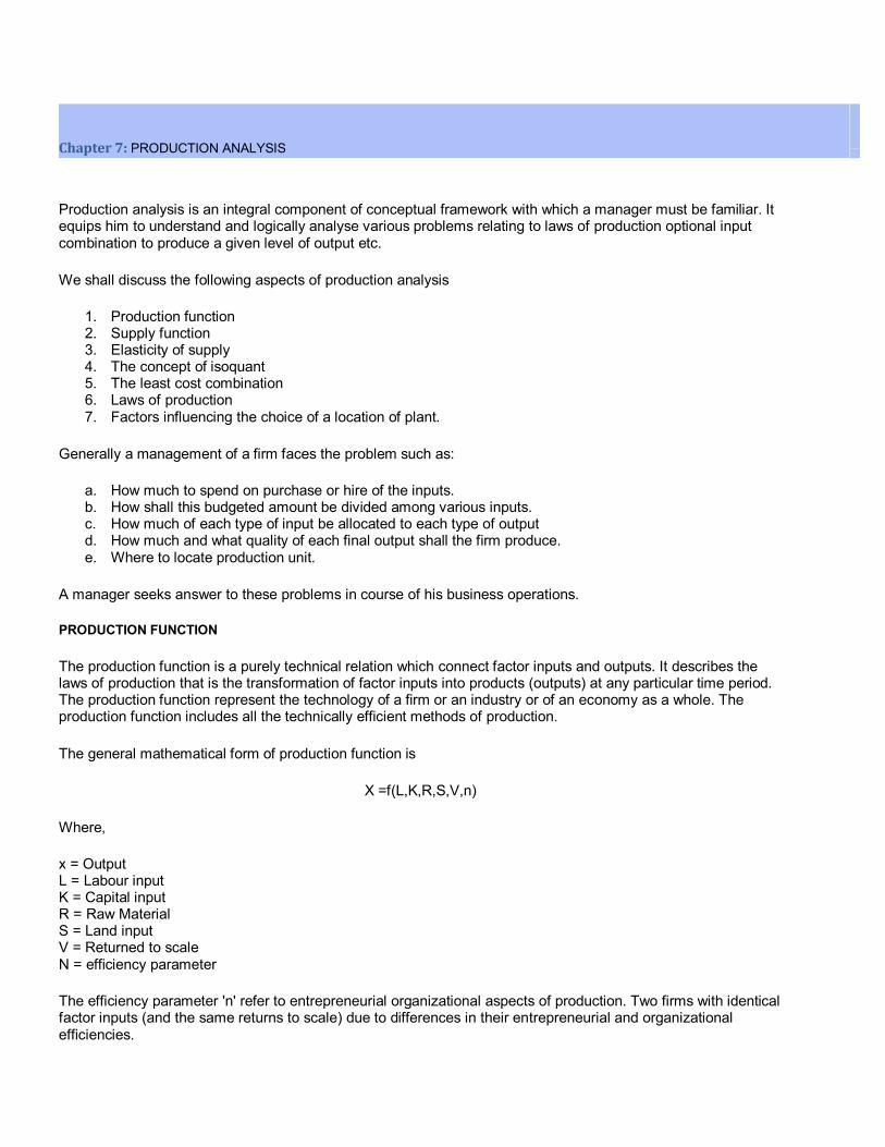
Chapter 7: PRODUCTION ANALYSIS

Production analysis is an integral component of conceptual framework with which a manager must be familiar. It equips him to understand and logically analyse various problems relating to laws of production optional input combination to produce a given level of output etc.

We shall discuss the following aspects of production analysis

1. Production function 2. Supply function 3. Elasticity of supply 4. The concept of isoquant 5. The least cost combination 6. Laws of production 7. Factors influencing the choice of a location of plant.

Generally a management of a firm faces the problem such as:

a. How much to spend on purchase or hire of the inputs. b. How shall this budgeted amount be divided among various inputs. c. How much of each type of input be allocated to each type of output d. How much and what quality of each final output shall the firm produce. e. Where to locate production unit.

A manager seeks answer to these problems in course of his business operations.

PRODUCTION FUNCTION

The production function is a purely technical relation which connect factor inputs and outputs. It describes the laws of production that is the transformation of factor inputs into products (outputs) at any particular time period. The production function represent the technology of a firm or an industry or of an economy as a whole. The production function includes all the technically efficient methods of production.

The general mathematical form of production function is

X =f(L,K,R,S,V,n)

Where,

x = Output L = Labour input K = Capital input R = Raw Material S = Land input V = Returned to scale N = efficiency parameter

The efficiency parameter 'n' refer to entrepreneurial organizational aspects of production. Two firms with identical factor inputs (and the same returns to scale) due to differences in their entrepreneurial and organizational efficiencies.

The production function is technology specific that with a change in technology, production function also changes.

The production function in traditional economic theory assumes the following form

x = F(L,K,V,n)

Ceteris paribus, the marginal product (MP) of factor is defined as the change in output (x) resulting from a (very small) change in the factor of production.

Mathematically the marginal product of each factor is the partial derivative of production function with respect to

a factor i.e.

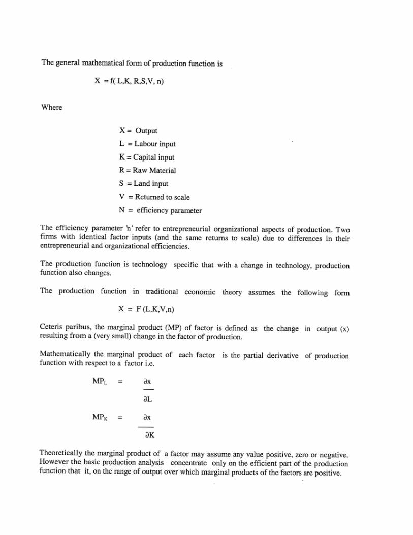
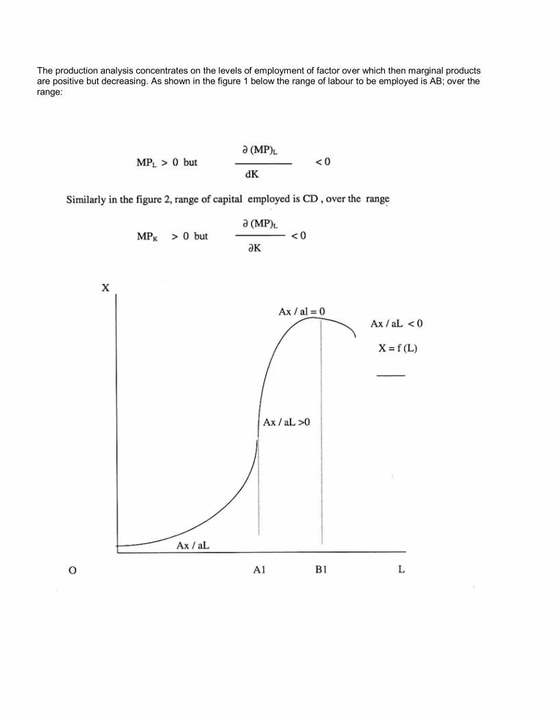
The production analysis concentrates on the levels of employment of factor over which then marginal products are positive but decreasing. As shown in the figure 1 below the range of labour to be employed is AB; over the range:

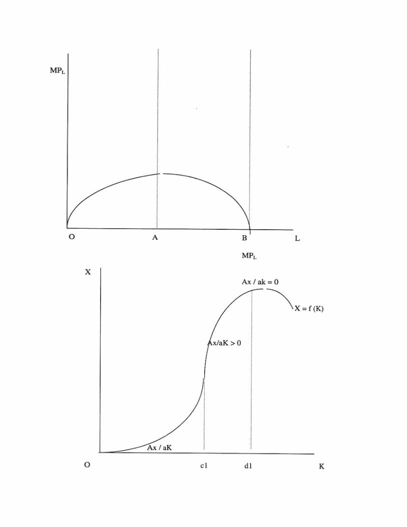
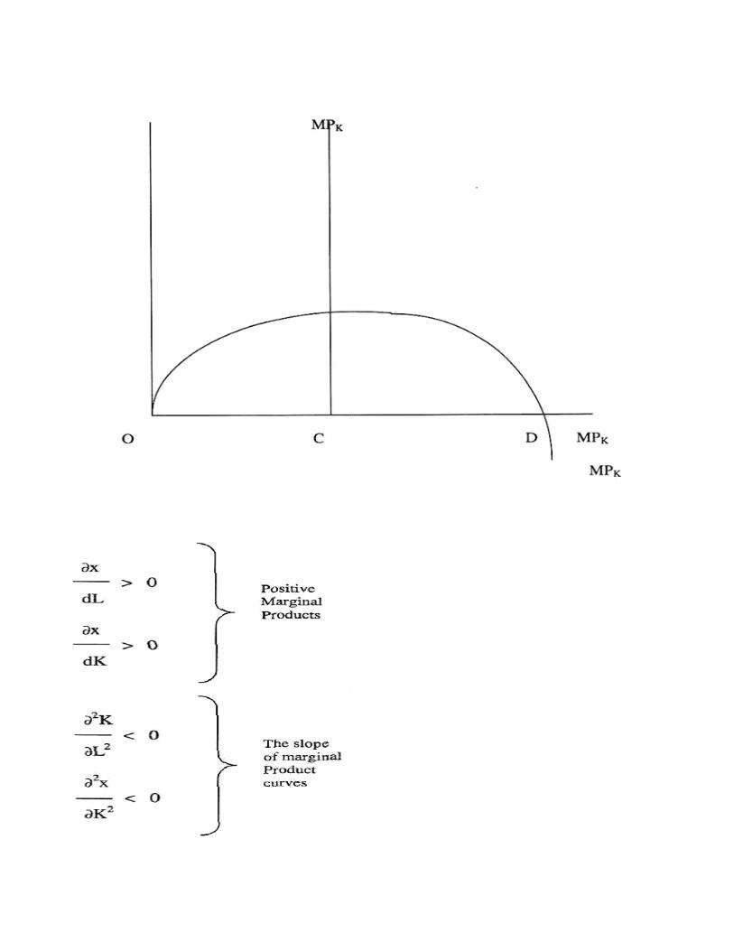
These conditions imply that the traditional theory f production concentrates on the range of isoquants over which their slope is negative and convex to the origin. COBB -DOUBLAS PRODUCTION FUNCTIONS

This is the most popular form of production function. The main reasons for its popularity are certain interesting properties that this function possess as well as the computational ease in its empirical estimation. CW Cobb and PH Douglas developed this function for estimating the relationship between inputs and outputs in manufacturing industry, though now used by analysis in almost all the fields of production including agriculture and transport.

The general from of Cobb -Douglas production function may be described as:

X = A La KP U

Where

X refers to level of output.

L refers to capital

A is a constant

U is a disturbance term

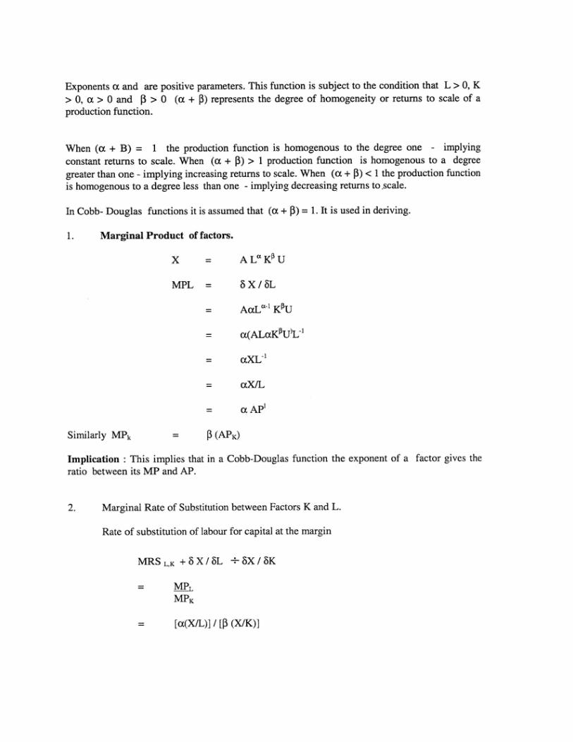
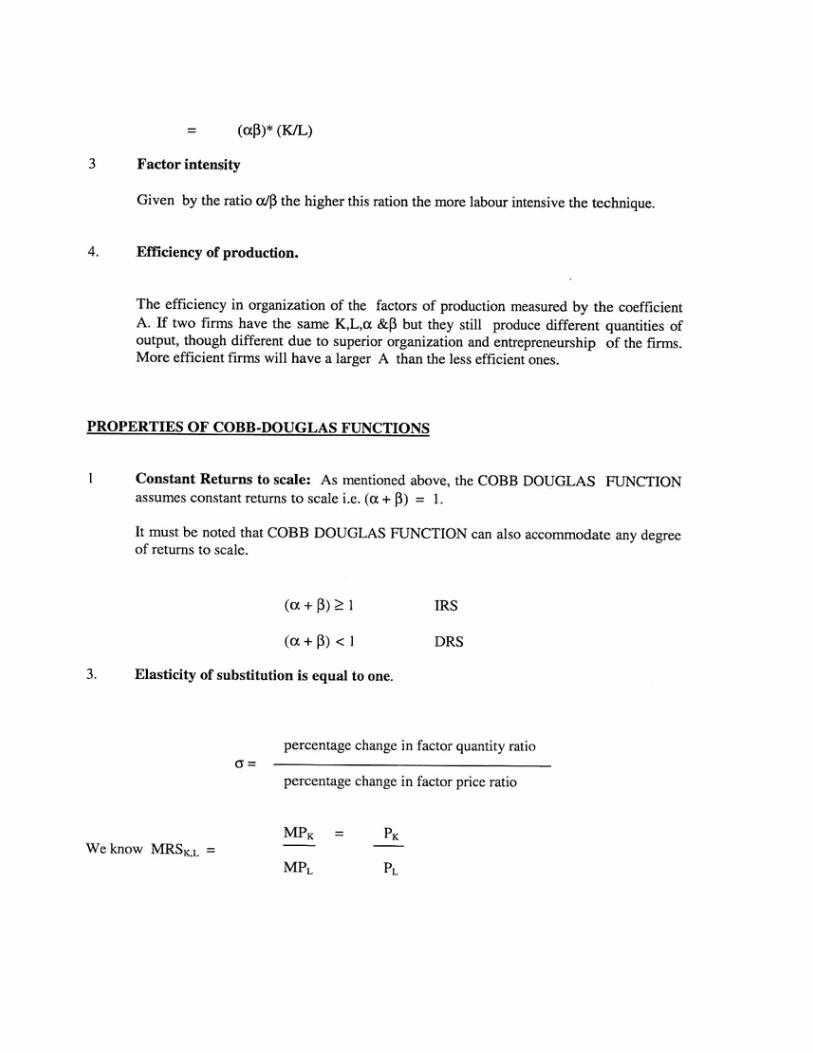
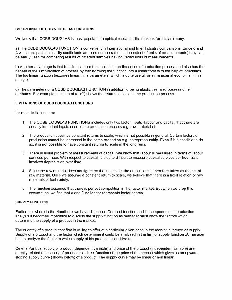
IMPORTANCE OF COBB-DOUGLAS FUNCTIONS

We know that COBB DOUGLAS is most popular in empirical research; the reasons for this are many:

a) The COBB DOUGLAS FUNCTION is convenient in International and Inter Industry comparisons. Since α and ß which are partial elasticity coefficients are pure numbers (i.e., independent of units of measurements) they can be easily used for comparing results of different samples having varied units of measurements.

b) Another advantage is that function capture the essential non-linearities of production process and also has the benefit of the simplification of process by transforming the function into a linear form with the help of logarithms. The log linear function becomes linear in its parameters, which is quite useful for a managerial economist in his analysis.

c) The parameters of a COBB DOUGLAS FUNCTION in addition to being elasticities, also possess other attributes. For example, the sum of (α +ß) shows the returns to scale in the production process.

LIMITATIONS OF COBB DOUGLAS FUNCTIONS

It's main limitations are:

1. The COBB DOUGLAS FUNCTIONS includes only two factor inputs -labour and capital, that there are equally important inputs used in the production process e.g. raw material etc.

2. The production assumes constant returns to scale, which is not possible in general. Certain factors of production cannot be increased in the same proportion e.g. entrepreneurship. Even if it is possible to do so, it is not possible to have constant returns to scale in the long runs,

3. There is usual problem of measurements of capital. We know that labour is measured in terms of labour services per hour. With respect to capital, it is quite difficult to measure capital services per hour as it involves depreciation over time.

4. Since the raw material does not figure on the input side, the output side is therefore taken as the net of raw material. Once we assume a constant return to scale, we believe that there is a fixed relation of raw materials of fuel variety.

5. The function assumes that there is perfect competition in the factor market. But when we drop this assumption, we find that α and ß no longer represents factor shares.

SUPPLY FUNCTION

Earlier elsewhere in the Handbook we have discussed Demand function and its components. In production analysis it becomes imperative to discuss the supply function as manager must know the factors which determine the supply of a product in the market.

The quantity of a product that firm is willing to offer at a particular given price in the market is termed as supply. Supply of a product and the factor which determine it could be analysed in the firm of supply function .A manager has to analyze the factor to which supply of his product is sensitive to.

Ceteris Paribus, supply of product (dependent variable) and price of the product (independent variable) are directly related that supply of product is a direct function of the price of the product which gives us an upward sloping supply curve (shown below) of a product. The supply curve may be linear or non linear.

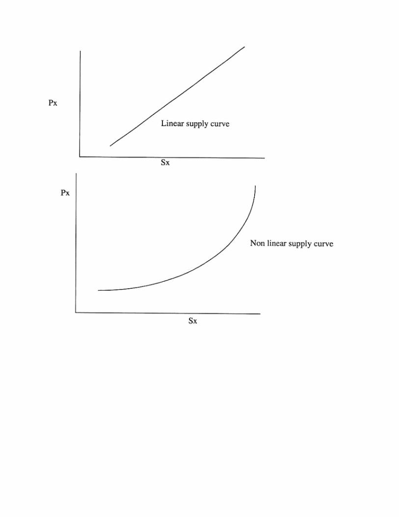
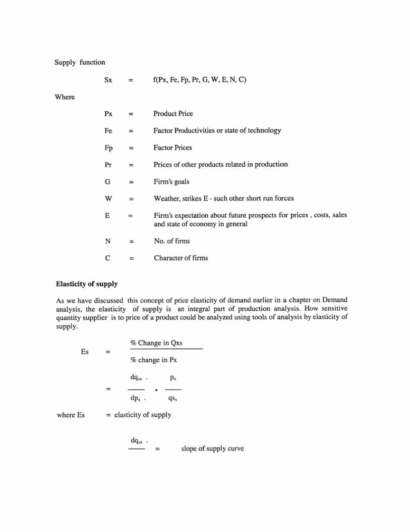
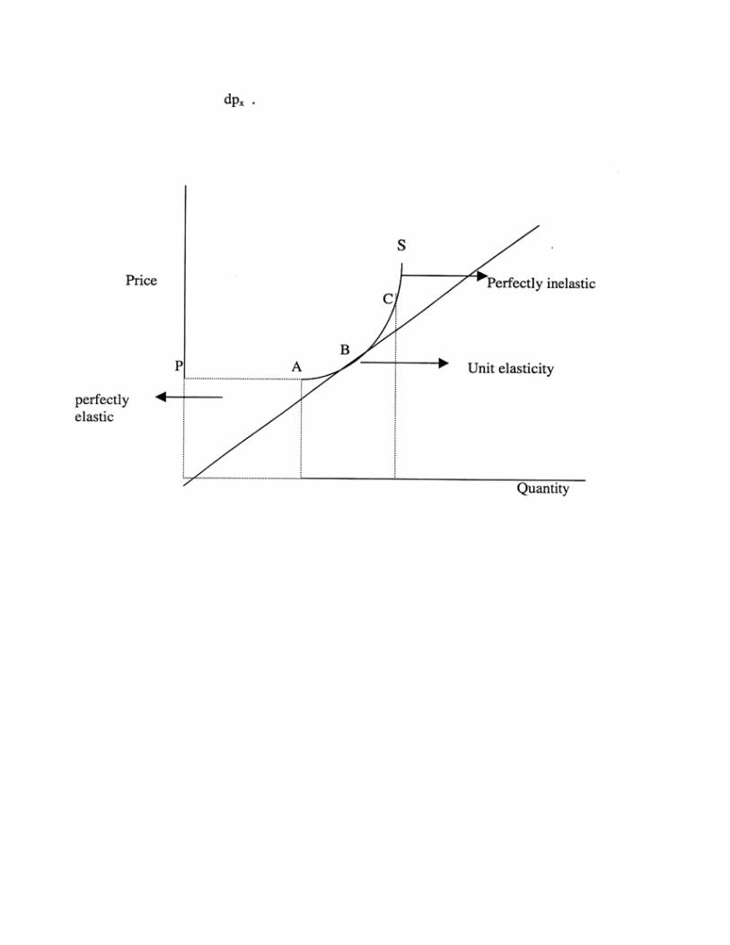
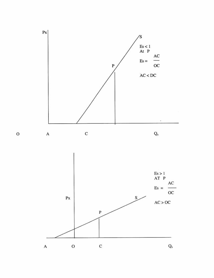
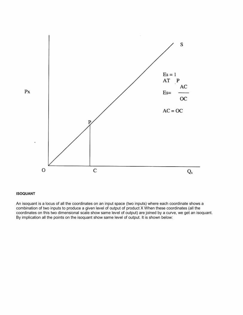
ISOQUANT

An isoquant is a locus of all the coordinates on an input space (two inputs) where each coordinate shows a combination of two inputs to produce a given level of output of product X When these coordinates (all the coordinates on this two dimensional scale show same level of output) are joined by a curve, we get an isoquant. By implication all the points on the isoquant show same level of output. It is shown below:

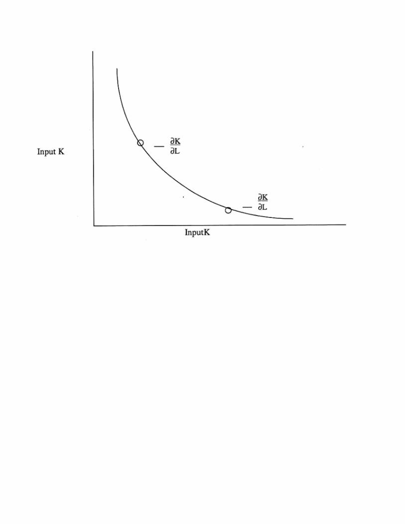
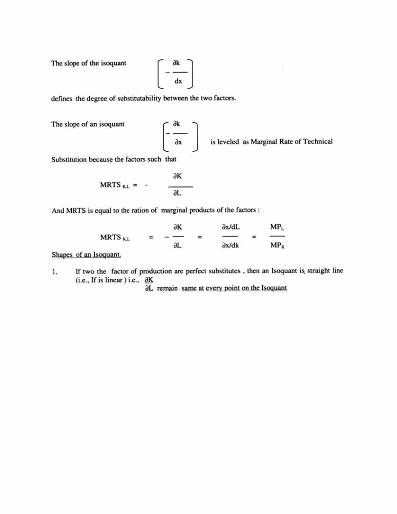
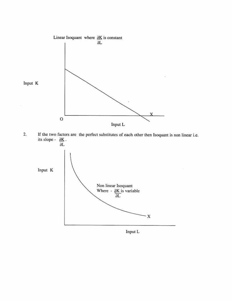
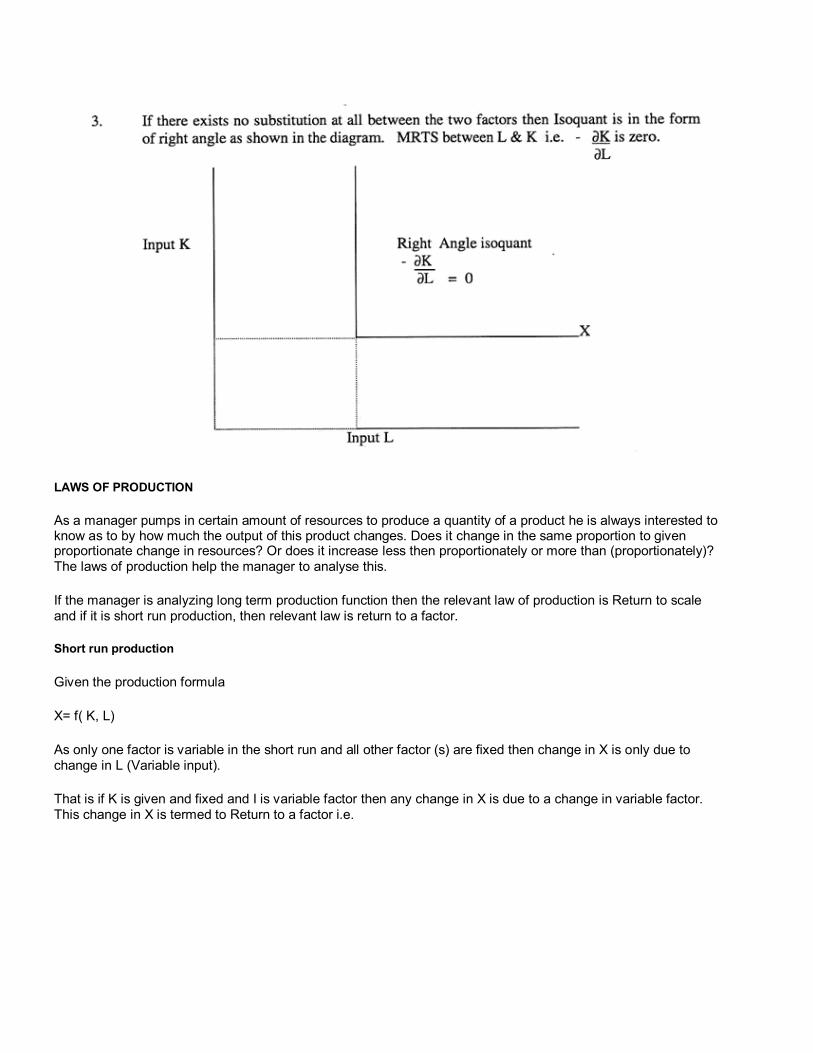
LAWS OF PRODUCTION

As a manager pumps in certain amount of resources to produce a quantity of a product he is always interested to know as to by how much the output of this product changes. Does it change in the same proportion to given proportionate change in resources? Or does it increase less then proportionately or more than (proportionately)? The laws of production help the manager to analyse this.

If the manager is analyzing long term production function then the relevant law of production is Return to scale and if it is short run production, then relevant law is return to a factor.

Short run production

Given the production formula

X= f( K, L)

As only one factor is variable in the short run and all other factor (s) are fixed then change in X is only due to change in L (Variable input).

That is if K is given and fixed and I is variable factor then any change in X is due to a change in variable factor. This change in X is termed to Return to a factor i.e.

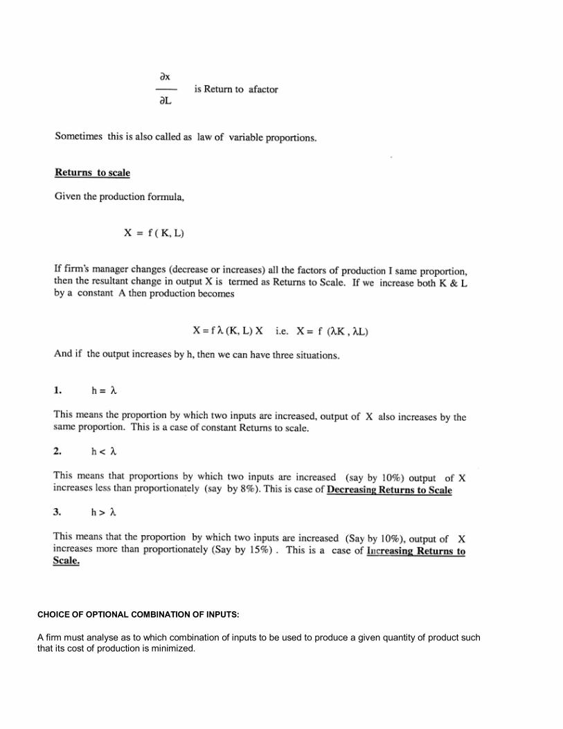
CHOICE OF OPTIONAL COMBINATION OF INPUTS:

A firm must analyse as to which combination of inputs to be used to produce a given quantity of product such that its cost of production is minimized.

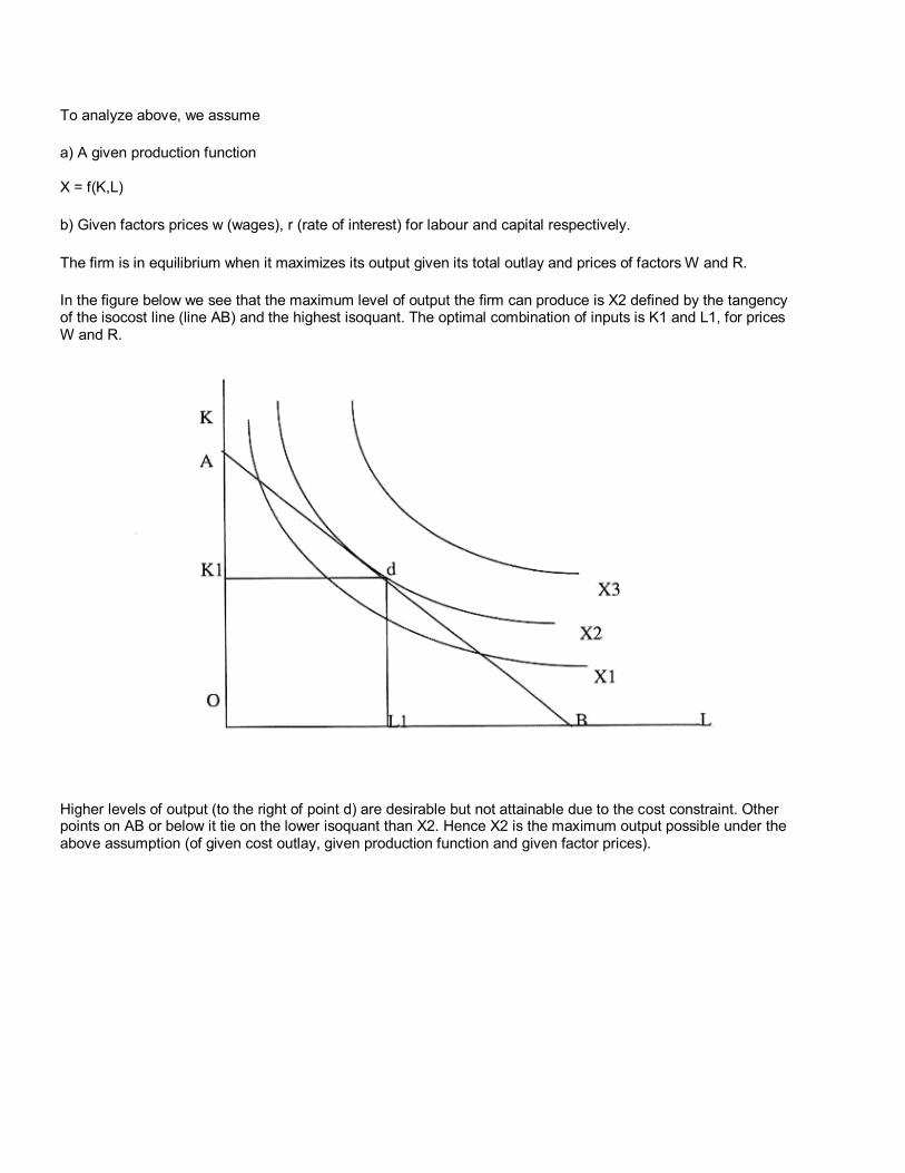
To analyze above, we assume

a) A given production function X = f(K,L)

b) Given factors prices w (wages), r (rate of interest) for labour and capital respectively.

The firm is in equilibrium when it maximizes its output given its total outlay and prices of factors W and R.

In the figure below we see that the maximum level of output the firm can produce is X2 defined by the tangency of the isocost line (line AB) and the highest isoquant. The optimal combination of inputs is K1 and L1, for prices W and R.

Higher levels of output (to the right of point d) are desirable but not attainable due to the cost constraint. Other points on AB or below it tie on the lower isoquant than X2. Hence X2 is the maximum output possible under the above assumption (of given cost outlay, given production function and given factor prices).

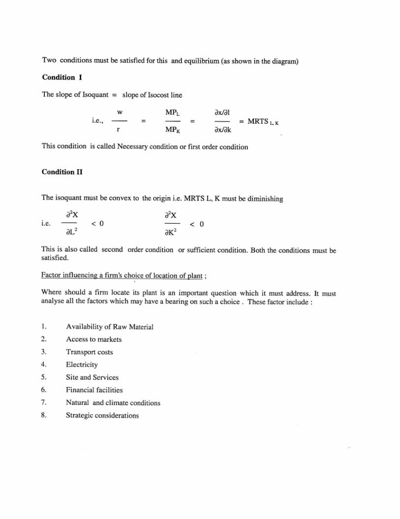
Chapter 8: PRICING AND OUTPUT DECISIONS UNDER DIFFERENT MARKET

STRUCTURES

The demand function, which the firm faces, which is an important determination of the price of the firm's product, is influenced significantly by the structure of market in which the firm operates. By market structure we mean the degree of competition in the market for the firm's goods or services. What would be the price of the product, the manager of a firm always have to keep in mind the nature of business he is operating. He would set a higher price of his product when he faces few sellers in the market and set a lower price when competitors are large in numbers.

The market structures could be classified as:

1. Perfect competition 2. Pure monopoly 3. Monopolistic competition 4. Monopoly 5. Bilateral Monopoly 6. Price Decision making monopoly 7. Oligopoly -various models.

Perfect competition: Price and Output decision.

It is a market which utopian in nature and as such exists rather rarely. It is studied more for its analytical value. It has the following characteristics:

1. There are large number of buyers and sellers.

2. Product is homogeneous

3. Neither the buyer nor the seller can influence the price of the produce. The firm is price taker and sells at market price over which it has no control. Similarly buyer also buys at a market price and has no influence on it. Thus price in the market is termed as EXOGENEOUS VARIABLE.

4. Any buyer or seller can enter or leave the market that there exists no restriction on the entry or exist of the firms/ buyers.

The equilibrium level of output and price in this market could be determined both in the short run as well as long run as explained in the example below:

Given the aggregate demand and supply function:

Aggregate Demand = Q = 25 -0.5 P Aggregate Supply = Q = 10 + 1.0 P

And cost function is given by

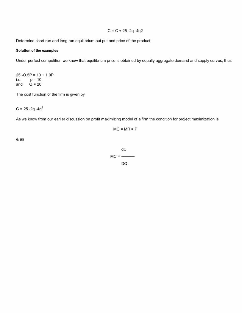
C = C + 25 -2q -4q2

Determine short run and long run equilibrium out put and price of the product;

Solution of the examples

Under perfect competition we know that equilibrium price is obtained by equally aggregate demand and supply curves, thus

25 -O.5P = 10 + 1.0P i.e. p = 10 and Q = 20

The cost function of the firm is given by

C = 25 -2q -4q

2

As we know from our earlier discussion on profit maximizing model of a firm the condition for project maximization is

MC = MR = P

& as

MC =

dC

______

DQ

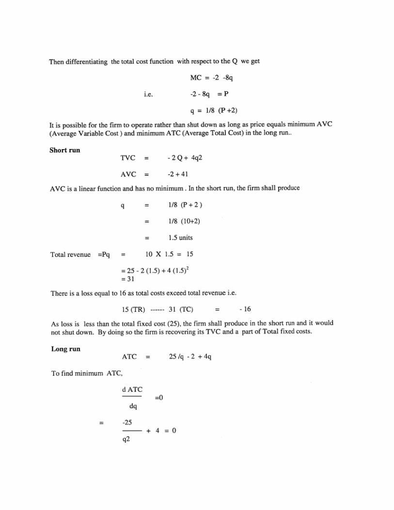
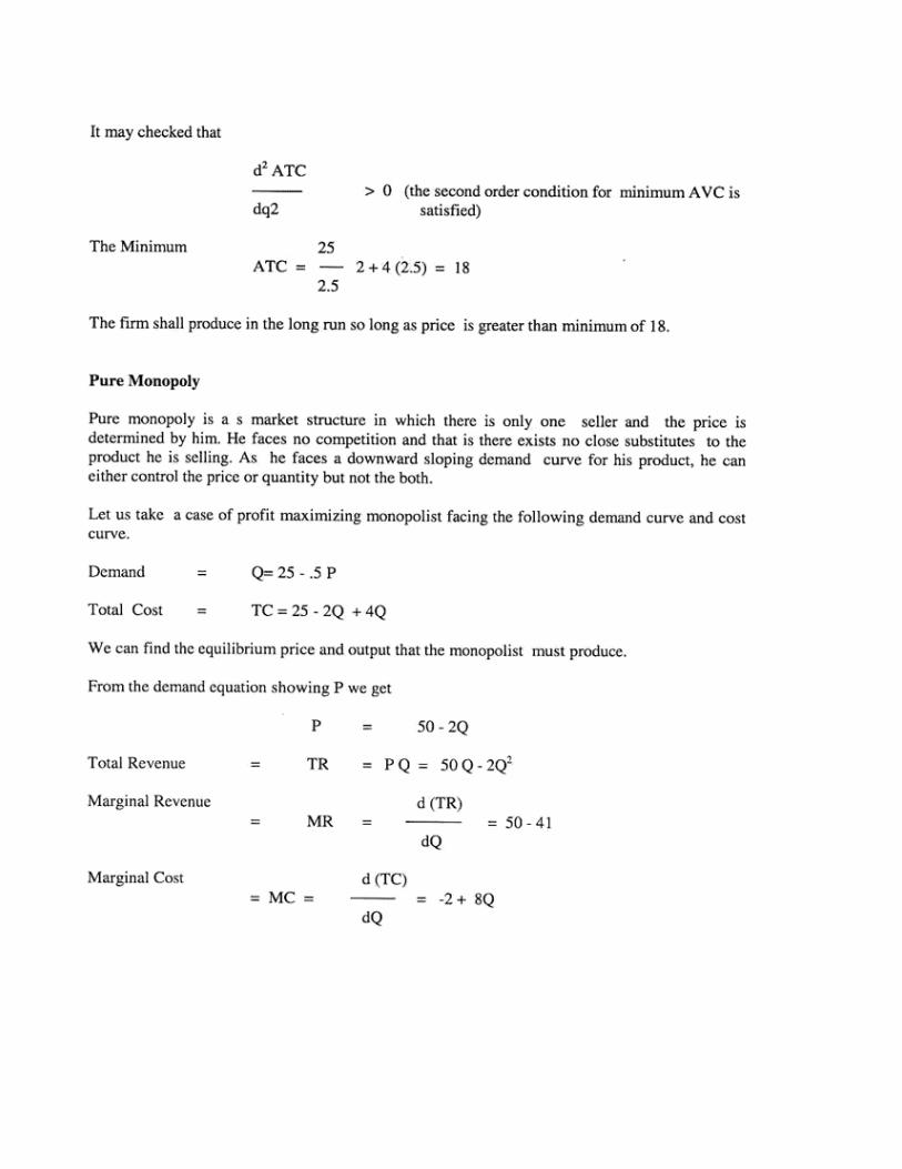
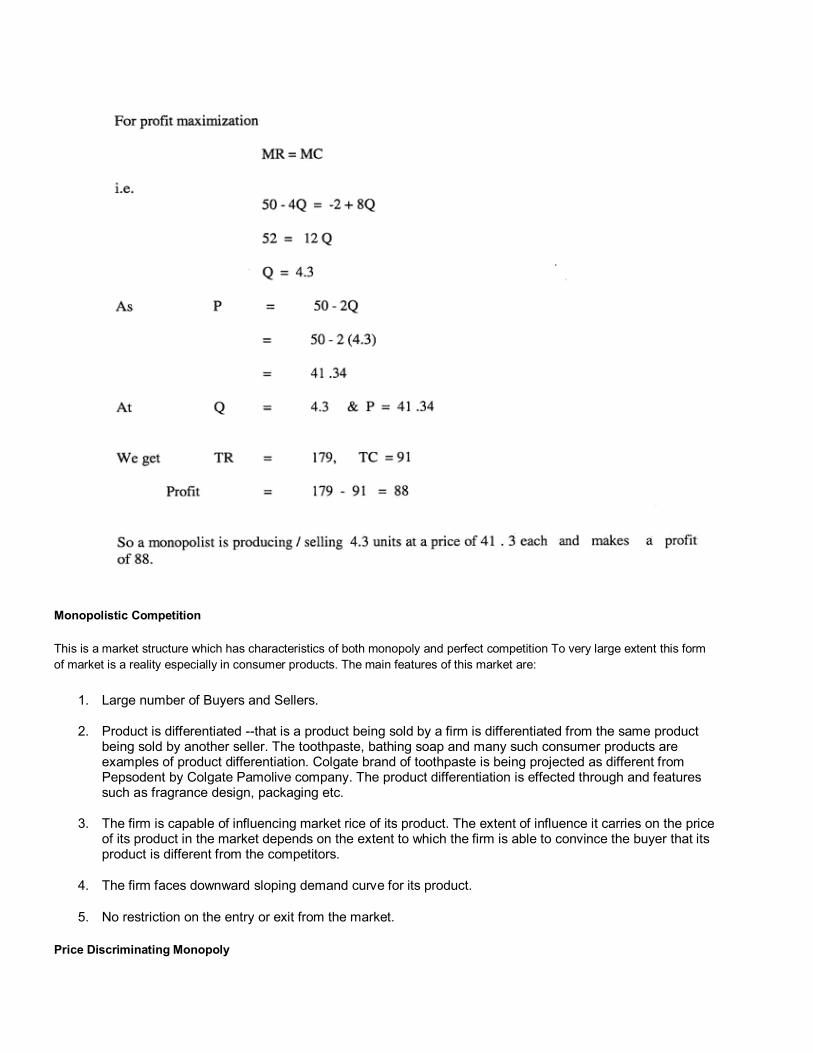
Monopolistic Competition

This is a market structure which has characteristics of both monopoly and perfect competition To very large extent this form

of market is a reality especially in consumer products. The main features of this market are:

1. Large number of Buyers and Sellers.

2. Product is differentiated --that is a product being sold by a firm is differentiated from the same product being sold by another seller. The toothpaste, bathing soap and many such consumer products are examples of product differentiation. Colgate brand of toothpaste is being projected as different from Pepsodent by Colgate Pamolive company. The product differentiation is effected through and features such as fragrance design, packaging etc.

3. The firm is capable of influencing market rice of its product. The extent of influence it carries on the price of its product in the market depends on the extent to which the firm is able to convince the buyer that its product is different from the competitors.

4. The firm faces downward sloping demand curve for its product.

5. No restriction on the entry or exit from the market.

Price Discriminating Monopoly

When a monopolist is charging different prices for its product in two different markets he is termed as price discriminating monopolist.

To explain this let us take market A and Market B where is firm F is selling its product under the condition of monopoly If it charges P x A in market A & P x B in Market B and P x A > P x B then firm F is price discriminating monopolist.

Two conditions must be satisfied for this

I. Price elasticity of demand for product X must be higher in market B than in market A.

II. Resale of product from market B to Market A is not possible

Bilateral Monopoly

This is a market where both seller and buyer have monopoly power. For example when trade union and management negotiate a wage settlement, (both have a monopoly power and wage agreement is negotiated through collective bargaining.)

Monopsony

It is a market where buyer has a monopoly power and there are large number of sellers. A labour market where in firm is a is a employer and large no of labourers offering their services, an example of monopoly.

OLIOGOPOLISTIC MARKET

Oligopoly is synonymous with competition among the few. Markets are said to be oligopolistic whenever a small number of firm's supply the dominant share of an industry's total output. In oligopoly, firms are large relative to the size of the total market they serve, and in the case of giant corporations they are large not just relatively but absolutely as well.

Characteristic of Oligopoly:

1. Interdependence. The most important feature of oligopoly is the interdependencies in decision making of the few firms which comprise the industry. This is because when number of competitors is few, any change in price, output, product etc., by a firm will have a direct effect on the fortune of its rivals, which will then retaliate in changing their own prices, output or products as the case may be.

2. A great importance of advertising and selling costs under conditions of market situation characterized by oligopoly. It is only under oligopoly that advertising comes fully into its own. Under prefect competition, advertising by an individual firm is unnecessary in view of the fact that he can sell any amount of his product at the going price.

3. Group Behaviour. Further, another important feature of oligopoly is that for its proper solution analysis of group behaviour is important. Theories of perfect competition, monopoly and monopolistic competition (with a large number of firms) present no difficult problem of making suitable assumption about human behaviour. But the theory of oligopoly is a theory of group behaviour not of mass or individual behaviour and to assume profit miximizing behaviour on his part may not be very valid.

4. Indeterminateness of Demand Curve Facing an Oligopolist. Another important feature is the indeterminateness of the demand curve facing an oligoolist. The demand curve shows what amounts of his product a firm will be able to sell at various prices.

. Under oligopoly, a firm cannot assume that its rivals will keep their prices unchanged when it makes changes in its own price. As a result of this, the demand curve facing an oligopolistic firm loses its definiteness and determinateness.

An oligopolistic market has several other characteristics. To begin with, rivalry among the few may involve either standardized or dirrerentatiated products. If the firms in an industry produce a standardized product, the industry is called a pure oligopoly. The most common examples of virtually uniform products marketed under condition of oligopoly include steel, aluminum, lead, copper, cement, rayon, fuel oil, plywood, tin cans, newsprint, adhesives, product, the industry is called a differentiated oligopoly. The most visible differentiated oligopolies involve the production of automobiles, toothpaste, cereal, cigarettes, TV sets, electric razors, computers, fax machines, refrigerators, air conditioners, soft drinks, soap and beer.

FACTORS LEADING TO AN OLIGOPOLISTIC MARKET

1. Economies of large scale production: When a small number of firms produce enough to meet the entire demand of the market, at a lower cost, as against a large number of firms, which could have the same output amongst themselves.

2. Absolute cost advantages of existing firms: When a small number of firms operate at a very low cost compared to a large number of firms, they would have an advantage in terms of pricing. They can price the products low enough to make it impossible for the large number of firms to recover their costs.

3. Financial capital requirements: Some of the businesses have too large a financial capital requirement for entry. This would mean that the new firm should have adequate resources so as to sustain losses for the first few years.

4. Mergers and restricting competition: Mergers in an industry transform its structure in two ways: Firstly, mergers undermine competition; secondly, they lead to concentration of production.

5. Product differentiation: In some cases product differentiation provides important advantage to certain firm which manage to control a large proportion of total sales.

VARIOUS MODELS OF OLIGOPOLY MARKETS

1. Sweezy's model of kinky demand curve

2. Collusive Model (Cartels)

3. Price Leadership Model

Sweezy Model of Kinky Demand Curve

AT the very outset, it must be pointed out that Sweezy's model does not furnish a theory in technical sense. A theory consists of a set of generalizations which explain the phenomenon which exists and which predict the phenomenon which does not exist in away, Sweezy's model tends to predict (For the future) the phenomenon which exists (*in the present for example, it seeks to explain why, once a price output combination has been decided upon, it will not readily change. It does not attempt to explain how a price output decision has been attained initially,

Originally, the empirical findings by Paul Sweezy, R. L Hall, and C J Hitch brought out two striking features of an oligopoly industry: Price rigidity and price leadership. Price I many oligopolistic industry exhibits sometimes a remarkable degree of stability. The stickiness of oligopoly prices at a time when costs of production change, may suggest that in an oligopoly market, price is not cost determined. Sometimes, price changes are determined by

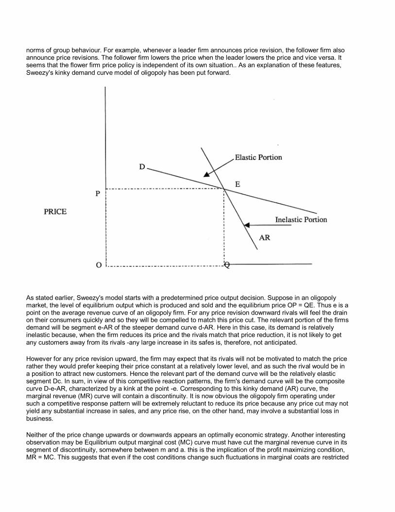
norms of group behaviour. For example, whenever a leader firm announces price revision, the follower firm also announce price revisions. The follower firm lowers the price when the leader lowers the price and vice versa. It seems that the flower firm price policy is independent of its own situation.. As an explanation of these features, Sweezy's kinky demand curve model of oligopoly has been put forward.

As stated earlier, Sweezy's model starts with a predetermined price output decision. Suppose in an oligopoly market, the level of equilibrium output which is produced and sold and the equilibrium price OP = QE. Thus e is a point on the average revenue curve of an oligopoly firm. For any price revision downward rivals will feel the drain on their consumers quickly and so they will be compelled to match this price cut. The relevant portion of the firms demand will be segment e-AR of the steeper demand curve d-AR. Here in this case, its demand is relatively inelastic because, when the firm reduces its price and the rivals match that price reduction, it is not likely to get any customers away from its rivals -any large increase in its safes is, therefore, not anticipated.

However for any price revision upward, the firm may expect that its rivals will not be motivated to match the price rather they would prefer keeping their price constant at a relatively lower level, and as such the rival would be in a position to attract new customers. Hence the relevant part of the demand curve will be the relatively elastic segment Dc. In sum, in view of this competitive reaction patterns, the firm's demand curve will be the composite curve D-e-AR, characterized by a kink at the point -e. Corresponding to this kinky demand (AR) curve, the marginal revenue (MR) curve will contain a discontinuity. It is now obvious the oligopoly firm operating under such a competitive response pattern will be extremely reluctant to reduce its price because any price cut may not yield any substantial increase in sales, and any price rise, on the other hand, may involve a substantial loss in business.

Neither of the price change upwards or downwards appears an optimally economic strategy. Another interesting observation may be Equilibrium output marginal cost (MC) curve must have cut the marginal revenue curve in its segment of discontinuity, somewhere between m and a. this is the implication of the profit maximizing condition, MR = MC. This suggests that even if the cost conditions change such fluctuations in marginal coats are restricted

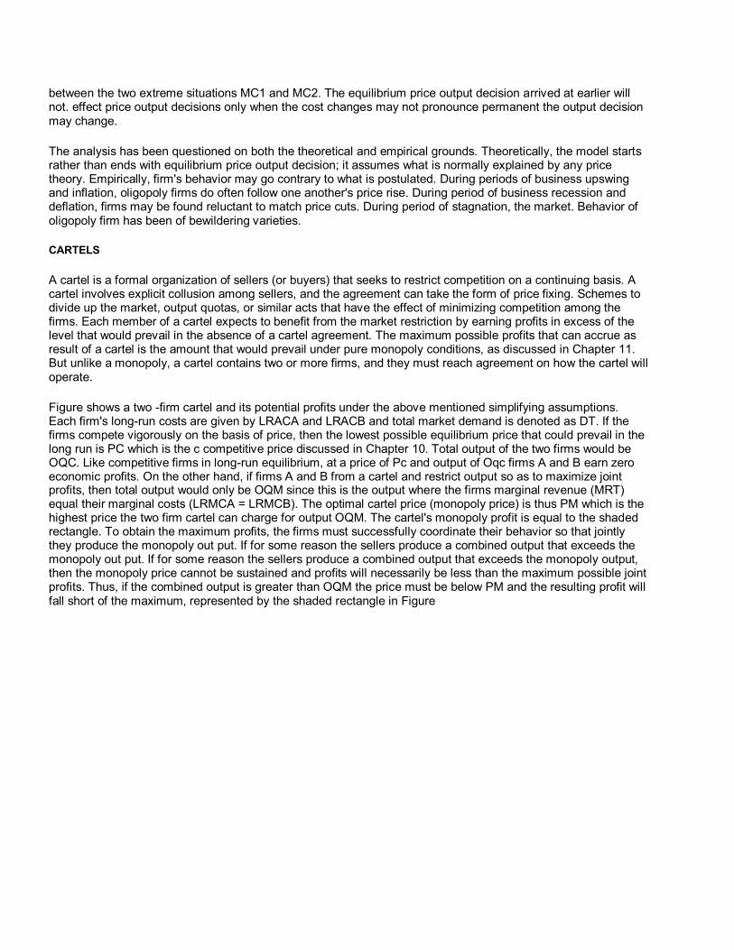
between the two extreme situations MC1 and MC2. The equilibrium price output decision arrived at earlier will not. effect price output decisions only when the cost changes may not pronounce permanent the output decision may change.

The analysis has been questioned on both the theoretical and empirical grounds. Theoretically, the model starts rather than ends with equilibrium price output decision; it assumes what is normally explained by any price theory. Empirically, firm's behavior may go contrary to what is postulated. During periods of business upswing and inflation, oligopoly firms do often follow one another's price rise. During period of business recession and deflation, firms may be found reluctant to match price cuts. During period of stagnation, the market. Behavior of oligopoly firm has been of bewildering varieties.

CARTELS

A cartel is a formal organization of sellers (or buyers) that seeks to restrict competition on a continuing basis. A cartel involves explicit collusion among sellers, and the agreement can take the form of price fixing. Schemes to divide up the market, output quotas, or similar acts that have the effect of minimizing competition among the firms. Each member of a cartel expects to benefit from the market restriction by earning profits in excess of the level that would prevail in the absence of a cartel agreement. The maximum possible profits that can accrue as result of a cartel is the amount that would prevail under pure monopoly conditions, as discussed in Chapter 11. But unlike a monopoly, a cartel contains two or more firms, and they must reach agreement on how the cartel will operate.

Figure shows a two -firm cartel and its potential profits under the above mentioned simplifying assumptions. Each firm's long-run costs are given by LRACA and LRACB and total market demand is denoted as DT. If the firms compete vigorously on the basis of price, then the lowest possible equilibrium price that could prevail in the long run is PC which is the c competitive price discussed in Chapter 10. Total output of the two firms would be OQC. Like competitive firms in long-run equilibrium, at a price of Pc and output of Oqc firms A and B earn zero economic profits. On the other hand, if firms A and B from a cartel and restrict output so as to maximize joint profits, then total output would only be OQM since this is the output where the firms marginal revenue (MRT) equal their marginal costs (LRMCA = LRMCB). The optimal cartel price (monopoly price) is thus PM which is the highest price the two firm cartel can charge for output OQM. The cartel's monopoly profit is equal to the shaded rectangle. To obtain the maximum profits, the firms must successfully coordinate their behavior so that jointly they produce the monopoly out put. If for some reason the sellers produce a combined output that exceeds the monopoly out put. If for some reason the sellers produce a combined output that exceeds the monopoly output, then the monopoly price cannot be sustained and profits will necessarily be less than the maximum possible joint profits. Thus, if the combined output is greater than OQM the price must be below PM and the resulting profit will fall short of the maximum, represented by the shaded rectangle in Figure

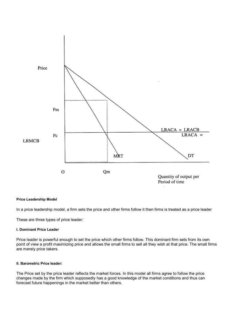
Price Leadership Model

In a price leadership model, a firm sets the price and other firms follow it then firms is treated as a price leader

These are three types of price leader:

I. Dominant Price Leader

Price leader is powerful enough to set the price which other firms follow. This dominant firm sets from its own point of view a profit maximizing price and allows the small firms to sell all they wish at that price. The small firms are merely price takers.

II. Barometric Price leader:

The Price set by the price leader reflects the market forces. In this model all firms agree to follow the price changes made by the firm which supposedly has a good knowledge of the market conditions and thus can forecast future happenings in the market better than others.

III. Price leadership by a low cost firm:

In an oligopolistic market sometimes price is set by the most efficient or the low cost firm and although other firms do not maximize their profits at their price, yet they have no choice but to accept it.

1. Price Leadership arises due to

2. Lower cost and enough financial resources.

3. Substantial share of market.

4. A firm having reputation for sound pricing decisions

5. Aggressive pricing

CHARACTERISTIC FEATURES OF PRICE LEADERSHIP

Price leaders aim at making few but larger & dramatic price change.

Normally the price leader leads only in Price rise.

Price leader must be ready to take the risk of price war in order to establish and maintain leadership

Price leader must pursue a definite and consistent pricing policy

Price leader plays important role in forecasting demand and cost conditions.

The sales of an 'Ideal' price leader are not much effected if the follower does not follow suit in case of price rise.