Accuracy and Stability Analysis of Path Loss Exponent ...

Accuracy and Stability Analysis of Path Loss Exponent Measurement for Localization in Wireless Sensor Network

1 Chuan Chin Pu, 2 Pei Cheng Ooi, 3 Wan-Young Chung *1 Sunway University, Malaysia, [email protected]

2 The University of Nottingham Malaysia Campus, [email protected] 3 Pukyong National University, South Korea, [email protected]

Abstract

In wireless sensor network localization, path loss model is often used to provide a conversion between distance and received signal strength (RSS). Path loss exponent is one of the main environmental parameters for path loss model to characterize the rate of conversion. Therefore, the accuracy of path loss exponent directly influences the results of RSS-to-distance conversion. When the conversion requires distance estimation from RSS value, small error of measured path loss exponent could lead to large error of the conversion output. To improve the localization results, the approaches of measuring accurate parameters from different environments have become important. Different approaches provide different measurement stabilities, depending on the performance and robustness of the approach. This paper presents four calibration approaches to provide measurements of path loss exponent based on measurement arrangement and transmitter/receiver node’s allocation. These include one-line measurement, online-update spread locations measurement, online-update small-to-big rectangular measurement, and online-update big-to-small rectangular measurement. The first two are general approaches, and the last two are our newly proposed approaches. Based on our research experiments, a comparison is presented among the four approaches in terms of accuracy and stability. The results show that both online-update rectangular measurements have better stability of measurements. For accuracy of measurement, online-update big-to-small rectangular measurement provides the best result after convergence.

Keywords: Calibration, Radio Ranging, Received Signal Strength

1. Introduction

Path loss model is an efficient and general approach to relate distance and received signal

strength in wireless sensor network (WSN) applications. This has been widely implemented in ranging, localization [1], and location tracking systems. Among the distance ranging techniques, radio ranging is widely accepted to be used in WSN. Radio ranging can be achieved through the measurement of physical change encountered during signal propagation [2][3]. Using received signal strength indicator (RSSI) measured at receiver, distance estimation between transmitter and receiver can be very easy and convenient.

Radio ranging using RSSI provides competitive advantages but further research is needed for improvement. For example, ranging result can be inaccurate and inconsistent especially in indoor environment [4]. In addition, multipath propagation happens frequently and seriously in an enclosed small room. Environmental changes such as temperature / humidity, human activities, and objects arrangement cause parameters deviation. All these problems are combined leading to the need of improvement in accurate radio ranging requirement.

Radio ranging using RSSI generally considers three models: small scale (spatial and temporal) multipath fading [5], medium scale (spatial) shadowing model [6], and large scale (spatial) path loss (PL) model [7]. The combination these there models [8] produces the modelling of the actual signal propagation under complicated environment. Among them, multipath fading effect is unwanted and can be mitigated by filters. Shadowing model explains the slow signal-strength fluctuation versus distance. This effect can be emulated by ray tracing methods [9]. The last model, path loss model is an empirical model which describes the attenuation of signal strength versus distance. A range of extension models [10] have been proposed to enhance the performance for various environments and applications. Nevertheless,

Accuracy and Stability Analysis of Path Loss Exponent Measurement for Localization in Wireless Sensor Network Chuan Chin Pu, Pei Cheng Ooi, Wan-Young Chung

International Journal of Digital Content Technology and its Applications(JDCTA) Volume7,Number7,April 2013 doi:10.4156/jdcta.vol7.issue7.136

1148

CORE Metadata, citation and similar papers at core.ac.uk

Provided by Sunway Institutional Repository

https://core.ac.uk/display/148366475?utm_source=pdf&utm_medium=banner&utm_campaign=pdf-decoration-v1

path loss exponent remains its significance as the main factor in the model regardless of how the model is varied.

RSSI ranging requires four basic stages: RSSI measurement, signal improvement, environmental characterization, and RSSI-to-distance conversion. To improve the accuracy of RSSI ranging, several ways can be considered by identifying the components that allow enhancement. Signal improvement provides enhancement through filtering noise and fast fading effect [11]. This increases the stability of the RSSI signal. RSSI-to-distance conversion can be enhanced in algorithm level [12]. Environmental characterization [13] provides measurement and calibration of path loss exponent. If the calibrated path loss exponent is accurate enough, the result obtained from RSSI-to-distance conversion becomes accurate [14][15]. Based on the nature as an exponent of the model, inaccurate path loss exponent amplifies the error if it is used to estimate distance from received signal strength. Therefore, measurement of accurate value for path loss exponent becomes very important as it directly influences the output of distance estimation.

The measurement of path loss exponent can be inaccurate and uncertain when direct wave of radio signal (line of sight, LOS) is weak while reflected waves are strong. The objective of this study is to find accurate path loss exponent under low propagation attenuation environment such as indoor places. Instead of investigating the calculation and processing of the RSSI for path loss exponent, we focus more on the arrangement of sensor nodes including the locations of transmitters and receivers.

2. Related works

Radio propagation and path loss models are well defined research topic with firm theoretical

background [16]. It leads to many location-related applications. From the algorithm aspect, [17] proposed three methods for large scale WSN. The first method uses mean interference, the second method is based on virtual outage probabilities, and the third one applies cardinality of the transmitting set. The experiments were based on a generic system model for simulation.

The estimation of path loss exponent relies on the measurements of the received signal strength together with the corresponding locations. However, accurate measurement of locations and distances could be difficult in some environments. Therefore, [15] proposed a continuous calibration scheme based on the Cayley-menger determinant. This method avoids distance measurement while performing path loss estimation in WSN. The main contribution which replaces location and distance measurement is using geometric constraints and the planarity of sensor networks. This paper induced other online calibration algorithms developed for path loss exponent estimation.

When localization technique is applied to mobile nodes, the estimation of the path loss estimation does not just depend on online-calibration techniques, but also Doppler Effect. [18] proposed a dynamic estimation method for path loss exponent measurement using both Doppler effect and RSSI. The strong point of this research is that the method is good in vehicular environment. This is good for distance estimation between vehicles.

Almost all researches are algorithm oriented for wireless ranging [19-21]. A relatively less number of research activities mentioned about the acquisition of practical samples. For a practical research done in [22], data collection and the procedures were stated clearly. In this study, the acquisition of signal strength values was done in two ways: track run measurement and single marker measurement. By knowing the pre-designed path and location spot, the estimation of the path loss exponent can be achieved with the pair values of RSSI and location coordinate.

3. Path loss model and ranging

RSSI value can be converted to received-power by applying offset to obtain the correct level: offsetRSSIRSSIP ii where Pi is the actual received power from transmitter node i. RSSIi is the measured RSSI value for transmitter node i. RSSIoffset is the offset found empirically.


1149

If RSSI ranging is used to measure the distances between transmitter and receiver, log-distance path loss model [7] is used to express the relationship between received power and the corresponding distance:

0100 log10)()(

d

dndPdP rr

where Pr(d) is the received power of the receiver measured at a distance d to the transmitter, which is expressed in dBm.

In path loss model, two important parameters are used to characterize environment: path loss exponent n and the received power Pr(d0). Pr(d0) is the measured received power at distance d0 to the transmitter. To characterize the environment for RSSI ranging, received power Pr(d0) is first measured by allocating a receiver d0 apart from the transmitter. d0 is generally fixed at 1 meter. After Pr(d0) is obtained, the receiver is moved to other locations randomly to measure the received power with the corresponding distance.

4. Path loss exponent estimation

In this paper, we investigated two types of method for path loss exponent estimation. One

method is to calculate the path loss exponent using a number of received powers and the corresponding distances. This method is called one-line measurement as the collection of RSSI values was done by locating the transmitter and receiver along a straight line, and varying the distance between them.

Another method is to directly update the environmental parameters using gradient decent technique. In this case, measurement of received power can be done in spread and random style as long as the exact locations in the area are known. This method is called online-update measurement as the environmental parameters such as path loss exponent can be updated continuously regardless of the change of environment.

For one-line measurement, received powers must be collected along the line with distance marked on the line. The collected RSSI values represent the received power at each marked distance along the line including the one-meter-place received power Pr(d0). When field measurement is done, the received powers (in dBm) are plotted in a graph versus distance. A straight line can be drawn along the received powers Pr(d) when the distance is using logarithmic scale:

010log10

d

dD

To find path loss exponent n, the gradient of the straight line is used:

0

min10

0

max10

maxmin

loglog10

)()(

d

d

d

d

dPrdPrn

Theoretically, every room/area has only one set of environmental parameters. However, the fact is that every location also has their own value although two locations are in the same area and they are neighbor. This can be verified when the measurement line is moved or rotated toward another direction, the estimation result will be slightly different. Note that a small change in path loss exponent n leads to drastic change in distance estimation.

The reason of this problem is the RSSI location-dependent variation especially in the medium scale spatial domain variation. Suppose we use uncertain and location-varied RSSI source for calculation, it is impossible that we are able to obtain accurate environmental parameters from inaccurate source. This causes different environmental parameters obtained at different locations. This indeed increases the difficulty of measuring accurate value of path loss exponent.

For online-update measurement, the measurement coordinates (x,y) must be predetermined. Three or four transmitters are required to be located in the area with coordinates (x1,y1), (x2,y2)


1150

and (x3,y3). If the distances d1, d2, and d3 between transmitters and receiver can be found using path loss model, the estimated location coordinate can be calculated using lateration:

2

32

32

3

22

22

22

21

21

21

yyxxd

yyxxd

yyxxd

By comparing the actual location coordinate with the estimated coordinate, the error between them can be found. However, it is highly unstable if we want to use the error to adjust the environmental parameters using gradient decent technique.

A more stable way is to find the calculated received power from predetermined location coordinates using both lateration and path loss RSSI-to-distance conversion. By comparing the calculated received power Pr(d) with the measured received power Pr’(d’), the error between them can be found and used in gradient decent adjustment:

)'(')( dPdPe rr To adjust path loss exponent n, the gradient vector is found using the mean-square error of the received powers:

010

2 log10)'(')(2d

ddPdPeE rrn

To adjust received power Pr(d0), the gradient vector is found using the mean-square error of the received powers:

)'(')(22 dPdPeE rrPr Recursive expressions can be used to update the parameters using the gradient vectors in (7) and (8):

21 2

1eEnn nkk

2001 2

1eEdPdP Prkrkr

where is the step size of the parameters. It controls the speed and stability of the convergence. This method provides global measurement for the environmental parameters as compared to

one-line measurement. This is because the measurement involves 3 or 4 transmitters at each corner of the measurement area. Therefore, the estimation result is valid for all locations within the whole area. 5. Data collection arrangement

In [19], two approaches of data collection were adopted: track run measurement and single

marker measurement. Although single marker measurement is done with selected locations without following a line, these approaches still remain at the ranging aspect. From localization aspect, the measurement should be done with all transmitters involved within the active area.

In this paper, we would like to propose a measurement arrangement so that the collected RSSI values provide global and accurate estimation for path loss exponent. In this case, it should implement online-update measurement approach for global validity. However, the online-update measurement still cannot provide optimized performance as different locations still can provide different accuracy.

Our proposed measurement arrangement tries to minimize the location error caused by location-dependent parameters. To achieve this objective, our proposed approach becomes greatly different from the ordinary arrangement. In our proposal, instead of changing the location of the receiver, it becomes stationary in our scenario. This means we have to change the location of the transmitters. The reason of keeping receiver stationary and changing the location of the transmitter is to create a condition so that the receiver always remains at the


1151

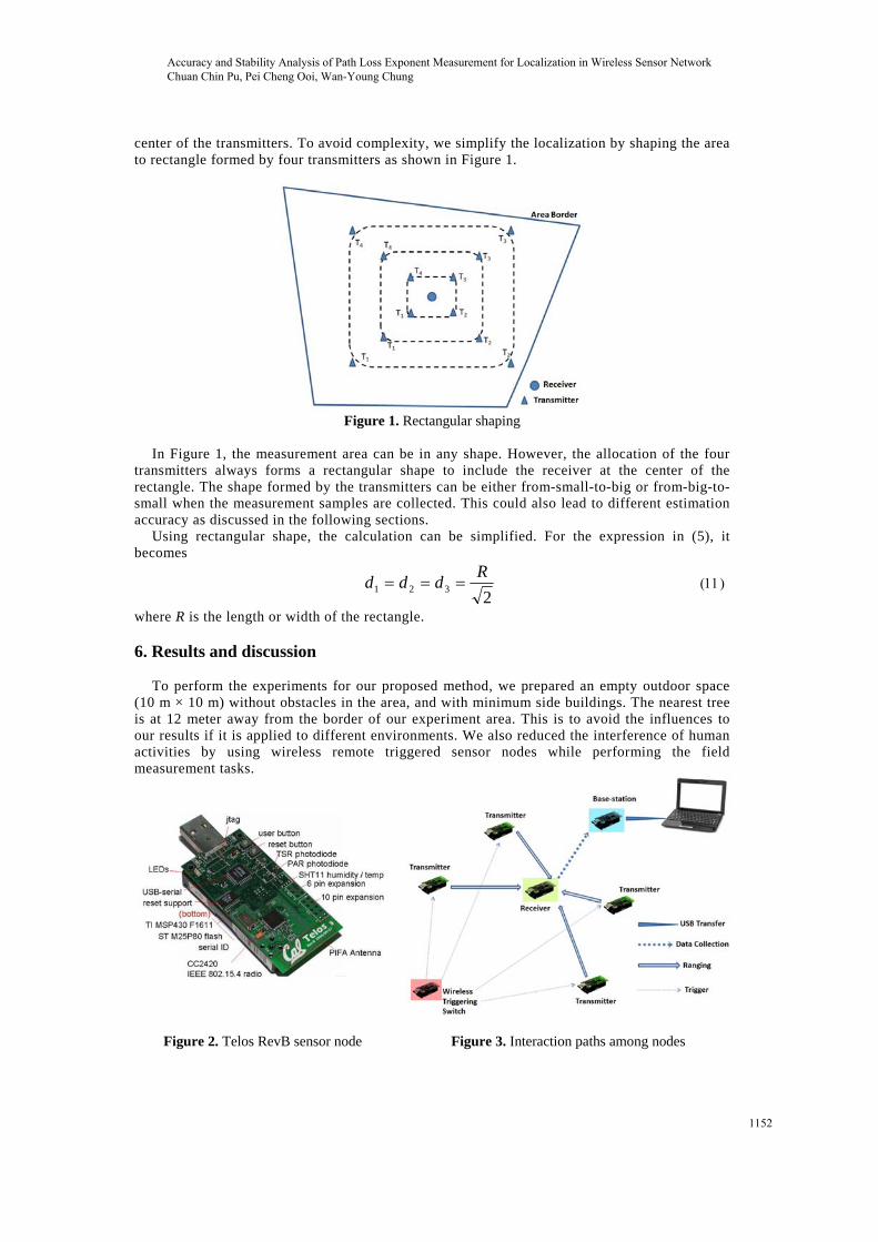
center of the transmitters. To avoid complexity, we simplify the localization by shaping the area to rectangle formed by four transmitters as shown in Figure 1.

Figure 1. Rectangular shaping

In Figure 1, the measurement area can be in any shape. However, the allocation of the four

transmitters always forms a rectangular shape to include the receiver at the center of the rectangle. The shape formed by the transmitters can be either from-small-to-big or from-big-to-small when the measurement samples are collected. This could also lead to different estimation accuracy as discussed in the following sections.

Using rectangular shape, the calculation can be simplified. For the expression in (5), it becomes

2

321

Rddd

where R is the length or width of the rectangle.

6. Results and discussion

To perform the experiments for our proposed method, we prepared an empty outdoor space (10 m × 10 m) without obstacles in the area, and with minimum side buildings. The nearest tree is at 12 meter away from the border of our experiment area. This is to avoid the influences to our results if it is applied to different environments. We also reduced the interference of human activities by using wireless remote triggered sensor nodes while performing the field measurement tasks.

Figure 2. Telos RevB sensor node Figure 3. Interaction paths among nodes


1152

In the experiments, Telos RevB wireless sensor nodes were programmed and used as transmitters and receiver as shown in Figure 2. Telos RevB implements IEEE 802.15.4 as its radio interface using CC2420 chip. The operational frequency falls at 2.4 GHz within the ISM band.

Besides the radio ranging between the transmitters and receiver, a sensor node was uniquely programmed to be given a special role as the wireless triggering switch. To trigger a ranging event, the user button shown in Figure 2 has to be pressed. This informs the node to send a triggering signal to the transmitters. The advantage of using a wireless triggering switch is that we are able to perform wireless ranging and path loss exponent measurement task from a remote distance. This helps to reduce the interference and influences caused by nearby human bodies.

During ranging task performed, 10 measurements were collected with every triggering signal given. These measured received signal strength values were averaged and transferred from the receiver to a base-station node attached to a computer. The computer has the main task to analyze and calculate the best estimated path loss exponent. The whole ranging process including signal trigger, ranging, and data collection path is illustrated in Figure 3.

In our experiment, we decided to perform both one-line measurement and online-update measurement. Under the category of online-update measurement, we performed three sub-tasks:

Sub-task 1: Predesigned spread locations measurement. Sub-task 2: From-small-to-big rectangular measurement. Sub-task 3: From-big-to-small rectangular measurement.

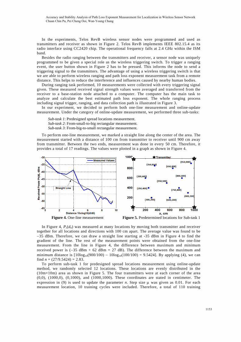
To perform one-line measurement, we marked a straight line along the center of the area. The measurement started with a distance of 100 cm from transmitter to receiver until 900 cm away from transmitter. Between the two ends, measurement was done in every 50 cm. Therefore, it provides a total of 17 readings. The values were plotted in a graph as shown in Figure 4.

Figure 4. One-line measurement

Figure 5. Predetermined locations for Sub-task 1

In Figure 4, Pr(d0) was measured at many locations by moving both transmitter and receiver together for all locations and directions with 100 cm apart. The average value was found to be 35 dBm. Therefore, we can draw a straight line starting at -35 dBm in Figure 4 to find the gradient of the line. The rest of the measurement points were obtained from the one-line measurement. From the line in Figure 4, the difference between maximum and minimum received power is (35 dBm + 62 dBm = 27 dB). The difference between the maximum and minimum distance is [10log10(900/100) 10log10(100/100) = 9.5424]. By applying (4), we can find n = (27/9.5424) = 2.83.

To perform sub-task 1 for predesigned spread locations measurement using online-update method, we randomly selected 12 locations. These locations are evenly distributed in the (10m×10m) area as shown in Figure 5. The four transmitters were at each corner of the area (0,0), (1000,0), (0,1000), and (1000,1000). These coordinates are stated in centimeter. The expression in (9) is used to update the parameter n. Step size was given as 0.01. For each measurement location, 10 training cycles were included. Therefore, a total of 110 training


1153

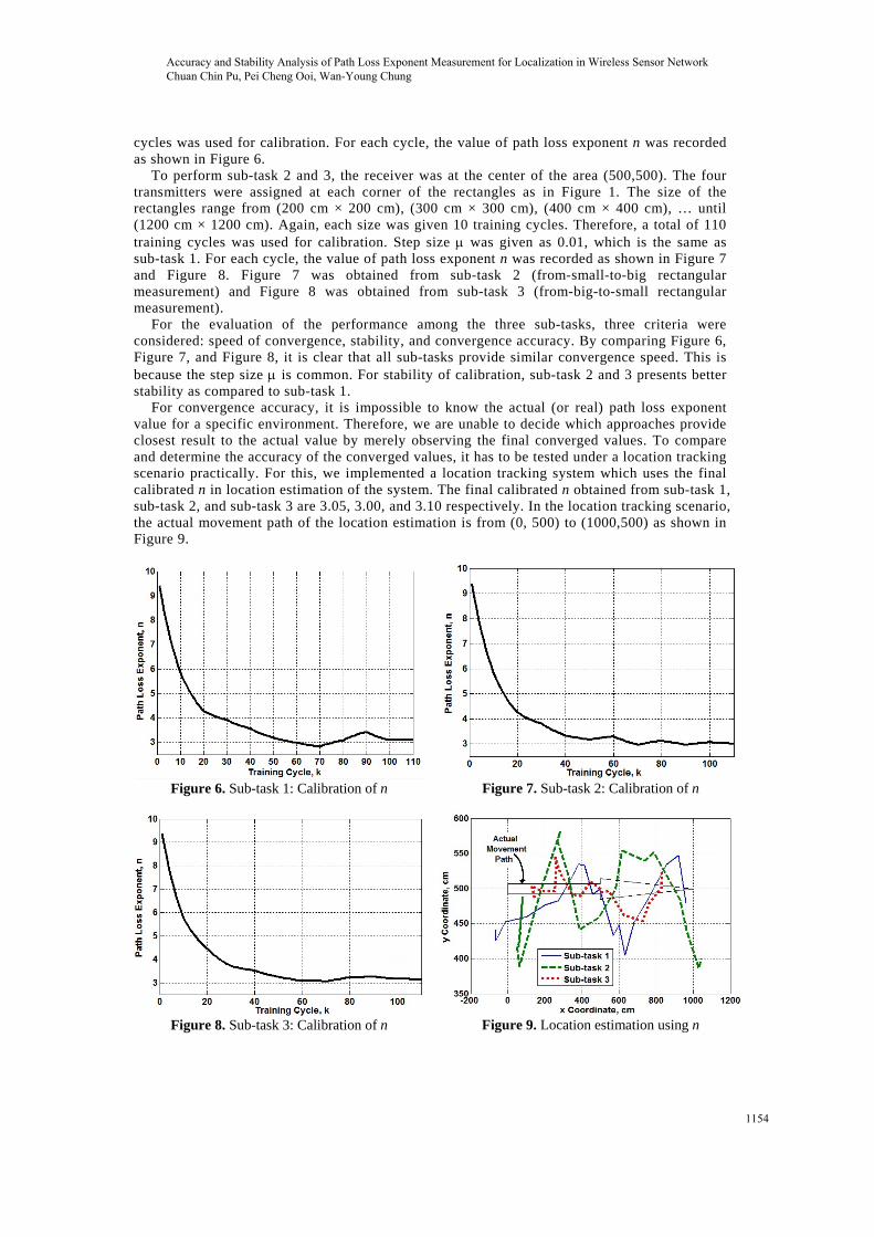
cycles was used for calibration. For each cycle, the value of path loss exponent n was recorded as shown in Figure 6.

To perform sub-task 2 and 3, the receiver was at the center of the area (500,500). The four transmitters were assigned at each corner of the rectangles as in Figure 1. The size of the rectangles range from (200 cm × 200 cm), (300 cm × 300 cm), (400 cm × 400 cm), … until (1200 cm × 1200 cm). Again, each size was given 10 training cycles. Therefore, a total of 110 training cycles was used for calibration. Step size was given as 0.01, which is the same as sub-task 1. For each cycle, the value of path loss exponent n was recorded as shown in Figure 7 and Figure 8. Figure 7 was obtained from sub-task 2 (from-small-to-big rectangular measurement) and Figure 8 was obtained from sub-task 3 (from-big-to-small rectangular measurement).

For the evaluation of the performance among the three sub-tasks, three criteria were considered: speed of convergence, stability, and convergence accuracy. By comparing Figure 6, Figure 7, and Figure 8, it is clear that all sub-tasks provide similar convergence speed. This is because the step size is common. For stability of calibration, sub-task 2 and 3 presents better stability as compared to sub-task 1.

For convergence accuracy, it is impossible to know the actual (or real) path loss exponent value for a specific environment. Therefore, we are unable to decide which approaches provide closest result to the actual value by merely observing the final converged values. To compare and determine the accuracy of the converged values, it has to be tested under a location tracking scenario practically. For this, we implemented a location tracking system which uses the final calibrated n in location estimation of the system. The final calibrated n obtained from sub-task 1, sub-task 2, and sub-task 3 are 3.05, 3.00, and 3.10 respectively. In the location tracking scenario, the actual movement path of the location estimation is from (0, 500) to (1000,500) as shown in Figure 9.

Figure 6. Sub-task 1: Calibration of n

Figure 7. Sub-task 2: Calibration of n

Figure 8. Sub-task 3: Calibration of n Figure 9. Location estimation using n


1154

The estimated traces of location tracking results were shown in Figure 9 for the three sub-tasks. From observation, the result obtained from sub-task 3 is less variation and fluctuation as compared to sub-task 1 and sub-task 2. Its trace is also closest to the actual movement path most of the time. Therefore, sub-task 3 can be considered to provide better accuracy for the converged path loss exponent. This shows that the convergence accuracy from sub-task 3 is better.

7. Conclusions

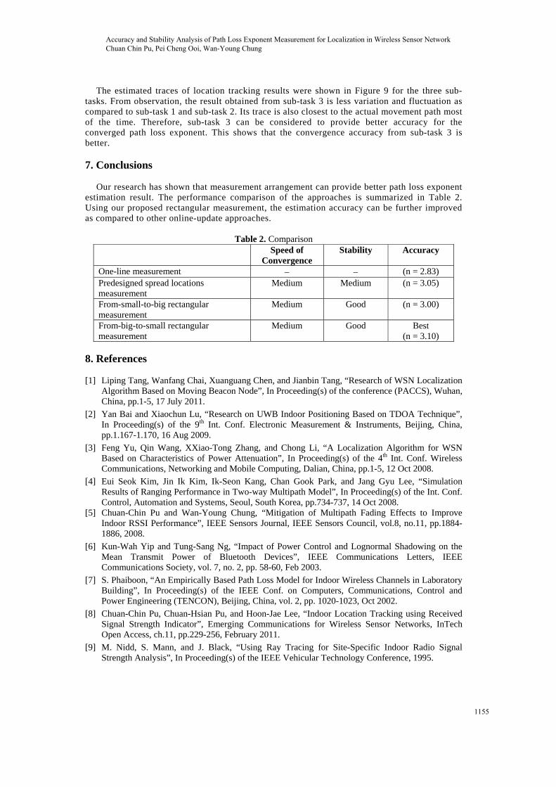
Our research has shown that measurement arrangement can provide better path loss exponent

estimation result. The performance comparison of the approaches is summarized in Table 2. Using our proposed rectangular measurement, the estimation accuracy can be further improved as compared to other online-update approaches.

Table 2. Comparison

Speed of Convergence

Stability Accuracy

One-line measurement (n = 2.83) Predesigned spread locations measurement

Medium Medium (n = 3.05)

From-small-to-big rectangular measurement

Medium Good (n = 3.00)

From-big-to-small rectangular measurement

Medium Good Best (n = 3.10)

8. References

[1] Liping Tang, Wanfang Chai, Xuanguang Chen, and Jianbin Tang, “Research of WSN Localization

Algorithm Based on Moving Beacon Node”, In Proceeding(s) of the conference (PACCS), Wuhan, China, pp.1-5, 17 July 2011.

[2] Yan Bai and Xiaochun Lu, “Research on UWB Indoor Positioning Based on TDOA Technique”, In Proceeding(s) of the 9th Int. Conf. Electronic Measurement & Instruments, Beijing, China, pp.1.167-1.170, 16 Aug 2009.

[3] Feng Yu, Qin Wang, XXiao-Tong Zhang, and Chong Li, “A Localization Algorithm for WSN Based on Characteristics of Power Attenuation”, In Proceeding(s) of the 4th Int. Conf. Wireless Communications, Networking and Mobile Computing, Dalian, China, pp.1-5, 12 Oct 2008.

[4] Eui Seok Kim, Jin Ik Kim, Ik-Seon Kang, Chan Gook Park, and Jang Gyu Lee, “Simulation Results of Ranging Performance in Two-way Multipath Model”, In Proceeding(s) of the Int. Conf. Control, Automation and Systems, Seoul, South Korea, pp.734-737, 14 Oct 2008.

[5] Chuan-Chin Pu and Wan-Young Chung, “Mitigation of Multipath Fading Effects to Improve Indoor RSSI Performance”, IEEE Sensors Journal, IEEE Sensors Council, vol.8, no.11, pp.1884-1886, 2008.

[6] Kun-Wah Yip and Tung-Sang Ng, “Impact of Power Control and Lognormal Shadowing on the Mean Transmit Power of Bluetooth Devices”, IEEE Communications Letters, IEEE Communications Society, vol. 7, no. 2, pp. 58-60, Feb 2003.

[7] S. Phaiboon, “An Empirically Based Path Loss Model for Indoor Wireless Channels in Laboratory Building”, In Proceeding(s) of the IEEE Conf. on Computers, Communications, Control and Power Engineering (TENCON), Beijing, China, vol. 2, pp. 1020-1023, Oct 2002.

[8] Chuan-Chin Pu, Chuan-Hsian Pu, and Hoon-Jae Lee, “Indoor Location Tracking using Received Signal Strength Indicator”, Emerging Communications for Wireless Sensor Networks, InTech Open Access, ch.11, pp.229-256, February 2011.

[9] M. Nidd, S. Mann, and J. Black, “Using Ray Tracing for Site-Specific Indoor Radio Signal Strength Analysis”, In Proceeding(s) of the IEEE Vehicular Technology Conference, 1995.


1155

[10] Samir M. Hameed, “Planning of WiMAX Networks Based on Modified Empirical Path Loss Model”, Journal of Communications and Information Sciences, AICIT, vol.2, no.1, pp.16-24, 2012.

[11] Xiaoyong Yan, HuanYan Qian, “RSSI based Positioning Error Ranging Removal of Mixed”, In Proceeding(s) of the Int. Conf. Consumer Electronics, Communications and Networks, Xianning, China, pp. 3498-3501, 16 April 2011.

[12] H. K. Maheshwari, A.H. Kemp, B. Peng, “Localization Performance Comparison using optimal and sub-optimal lateration in WSNs”, In Proceeding(s) of the 15th Asia-Pacific Conf. Communications, Shanghai, China, pp.842-845, 8 Oct 2009.

[13] Min Zhao, Muqing Wu, Deshui Yu, “Measurement and Characterization of The Near Ground Wideband Channel at 2.3GH”, JDCTA: International Journal of Digital Content Technology and its Applications, AICIT, vol.6, no. 21, pp.337-346, 2012.

[14] H. Alasti, Kunjie Xu, Zhe Dang, “Efficient experimental path loss exponent measurement for uniformly attenuated indoor radio channels”, In Proceeding(s) of the confeerence SOUTHEASTCON, Atlanta, GA, pp. 255-260, 5 March 2009.

[15] Guoqiang Mao, B.D.O. Anderson, B. Fidan, “WSN06-4: Online Calibration of Path Loss Exponent in Wireless Sensor Networks”, In Proceeding(s) of the conference Globecom, San Francisco, USA, pp. 1-6, 27 November 2006.

[16] Vijay Garg, Wireless Communications & Networking, ch.3, pp.47-81, Morgan Kaufmann, June 2007.

[17] S. Srinivasa and M. Haenggi, “Path Loss Exponent Estimation in Large Wireless Networks”, In Proceeding(s) of the conference CoRR., 4 February 2008

[18] N Alam, A.T. Balaie, and A.G. Dempster, “Dynamic Path Loss Exponent and Distance Estimation in a Vehicular Network using Doppler Effect and Received Signal Strength”, In Proceeding(s) of the IEEE Conf. Vehicular Technology, Ottawa, Canada, pp.1-5, 6 September 2010.

[19] Zhen-dong. Zeng, “The Research of Positioning Algorithm for Wireless Sensor Networks”, AISS: Advances in Information Sciences and Services Sciences, AICIT, vol.4, no.13, pp.16-22, 2012.

[20] Xiaoping Zhang, Yang Wang, Guixiong Liu, “Modeling Parameters Optimization for Target Localization in WSN Based on LSSVR by Sampling Measurement Data”, IJACT: International Journal of Advancements in Computing Technology, AICIT, vol.4, no.6, pp.346-357, 2012.

[21] Jie Chen, “RSSI-based Indoor Mobile Localization in Wireless Sensor Network”, JDCTA: International Journal of Digital Content Technology and its Applications, AICIT, vol.5, no.7, pp.407-416, 2011.

[22] Lorne Christopher Liechty, “Path Loss Measurement and model Analysis of a 2.4 GHZ Wireless Network in an Outdoor Environment”, Georgia Institute of Technology, August 2007.


1156

Accuracy and Stability Analysis of Path Loss Exponent ...

Documents