Accounting for Work Life Expectancy: Applying the Skoog ... for Work Life Expectancy... · in Skoog, Ciecka, and Krueger (2011) – hereinafter “S-C-K”. Less widely used are the

 © 2015

Accounting for Work Life Expectancy: Applying the Skoog-Ciecka-Krueger Transition Probabilities

David G. Tucek Value Economics, LLC

13024 Vinson Court St. Louis, MO 63043

Tel: 314/434-8633 Cell: 314/440-4925

[email protected]

Accepted for Publication in the

Journal of Legal Economics (forthcoming)

Abstract

While many forensic economists rely on the Skoog-Ciecka-Krueger work life tables, few seem to make

use of the labor force transition probabilities provided as supplemental material to the published tables.

This paper explains the calculations needed to compute the probability of labor force activity for a person

who is an initially active or an initially inactive labor force participant based on these transition

probabilities. Following this explanation, the explicit use of the probability of labor force activity is

compared to the common methods of accounting for work life expectancy. The paper concludes by

identifying the issues that use of the probability of labor force activity presents.

2  

Accounting for Work Life Expectancy:

Applying the Skoog-Ciecka-Krueger Transition Probabilities  

Journal of Legal Economics, 22(1) (forthcoming)

I Introduction

Many forensic economists recognize that future lost earnings will not be attained with certainty and

consequently reduce their loss estimates to account for the risk of death, injury, sickness and other events

that would keep an individual from being an active labor force participant. For example, in the 2012

Survey of Forensic Economists (Slesnick, Luthy and Brookshire, 2013), only 7.8 percent of the

respondents indicated they ended their loss calculation at some fixed retirement date; 3.0 percent used the

LPE method; and 70.3 percent of the remaining respondents indicated they relied on work life tables

published in economic journals. The latest such tables, and perhaps the most widely used, are those found

in Skoog, Ciecka, and Krueger (2011) – hereinafter “S-C-K”. Less widely used are the labor force

transition probabilities that were provided as supplemental materials to the S-C-K work life tables.

This paper presents the calculations required to compute the probability of labor force activity for persons

of a given age, gender, level of educational attainment and initial labor force status using the S-C-K

transition probabilities and extended versions of published life tables. Following this explanation, the

explicit use of the probability of labor force activity is compared to the common methods of accounting

for work life expectancy (WLE). The paper concludes by identifying the issues that use of the probability

of labor force activity presents.

II Required Calculations

Calculating the probability of being an active labor force participant is most easily understood in the

context of modeling the size of a synthetic cohort of initially active individuals as the cohort ages, while

at the same time calculating the number of deaths and the number of living inactive individuals. (For the

3  

corresponding probability of an initially inactive person, the modeled cohort corresponds to initially

inactive persons; the number of active persons and the number of deaths are also calculated.) This

approach is similar to the calculations underlying a period life table, in which the number of deaths and

remaining living persons from an initial cohort is calculated as the cohort ages. A specific example will

illustrate the calculation of the probability of being an active labor force participant.

Starting with 100,000 living females at age 30, the number of actives (A30) is set equal to 100,000, and the

number of living inactive (IA30) and deaths (D30) are both set equal to zero. At age 31, these values are

recalculated as follows:

(1) A31 = A30 ∙ aρa

30 + IA30 ∙ iρa

30 ;

(2) IA31 = A30 ∙ aρi

30 + IA30 ∙ iρi

30 ; and

(3) D31 = (A30 + IA30) ∙ (1 - l31/l30),

where aρax is the probability of someone who is age x transitioning from the active to the active state; iρa

x

is the probability of transitioning from the inactive to the active state; iρix is the probability of

transitioning from the inactive to the inactive state; aρix is the probability of transitioning from the active

to the inactive state; and where lx is the number of living persons age x taken from the life table. The aρax,

iρax , iρi

x , and aρix incorporate the probability of survival; that is, they are the S-C-K transition

probabilities multiplied by one minus the probability of death. Note that one minus lx/lx-1 equals the

probability of death.

At age 32, the values are recalculated again, as follows:

(1) A32 = A31 ∙ aρa

31 + IA31 ∙ iρa

31;

(2) IA32 = A31 ∙ aρi

31 + IA31 ∙ iρi

31; and

(3) D32 = (A31 + IA31) ∙ (1 - l32/l31).

These calculations are repeated for all subsequent ages through some terminal age after which no

remaining cohort members are active. The probability of being an active labor force participant at age x,

Px, is calculated as Ax divided by the initial size of the synthetic cohort (100,000). While it is not

4  

necessary to calculate the number of deaths in step (3), doing so allows one to check the calculations in

steps (1) and (2) since Dx+1 = lx - Ax+1 - IAx+1 for all ages.

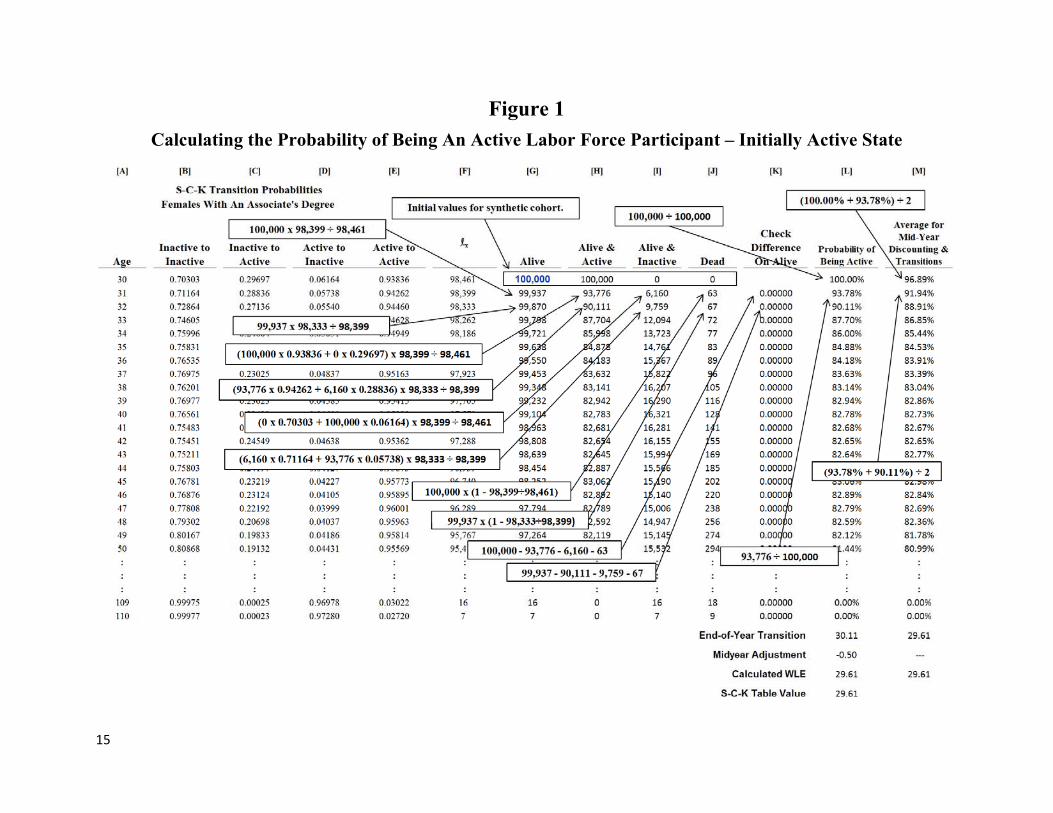
The required calculations are similar when the initial labor force status is inactive: the number of living

inactives (IA30) is set equal to 100,000, and the number of actives (A30) and deaths (D30) are both set equal

to zero. At age 31, and for all subsequent ages through the terminal age, these values are recalculated as

outlined above. The probability of being an active labor force participant at age x is still calculated as Ax

divided by the initial size of the synthetic cohort. This calculation is equivalent to one minus the sum of

IAx and the total cumulative deaths divided by the initial size of the synthetic cohort. Note that this sum

is the total number of inactive persons – both living and deceased – out of the initial cohort at age x.

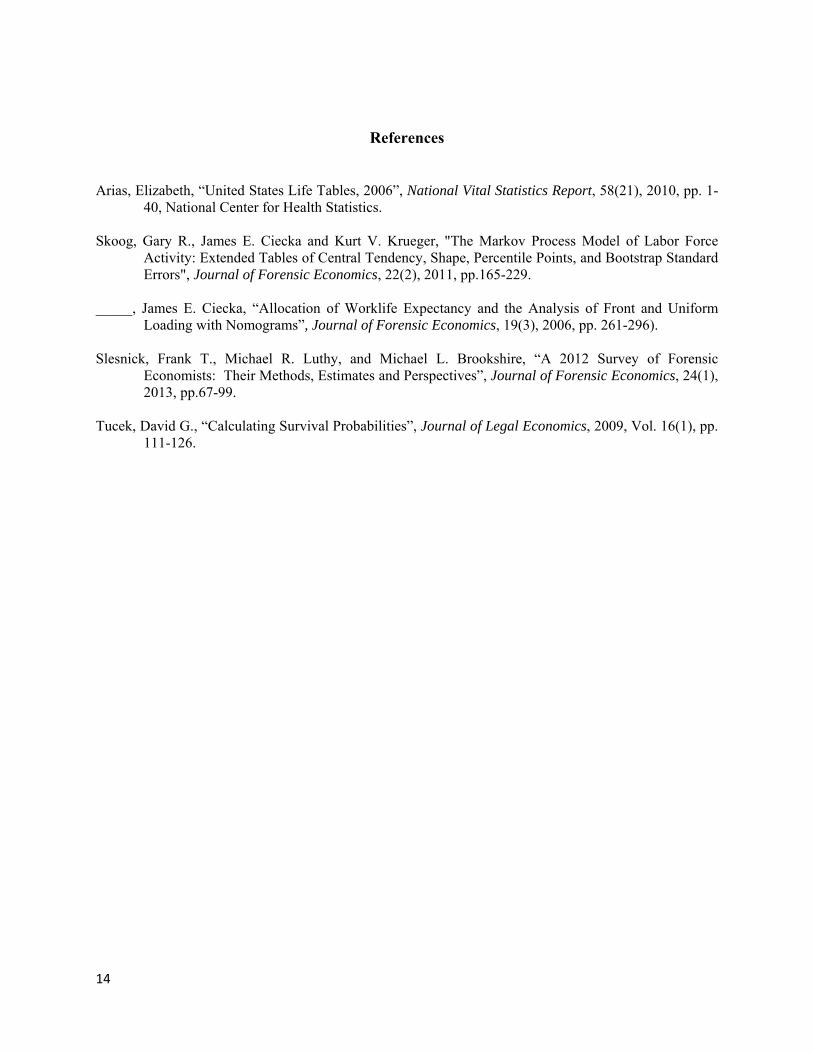
Figure 1 presents the calculation of the probability of labor force activity for an initially active 30-year

old female with an Associate’s degree in spreadsheet form. Figure 2 presents the corresponding

calculations for the initially inactive state. In both figures, columns B through E contain the S-C-K

transition probabilities for a female with an Associate’s degree from age 30 on; these probabilities are not

conditioned on the probability of survival. Column F contains the values of the lx from the 2006 life

tables for females.1 These values are used to calculate the number of survivors at each successive age in

column G, given the starting cohort value of 100,000. The number of survivors at age x+1 equals the

survivors at age x times the ratio of lx+1 to lx. This ratio equals the probability of a person age x living to

age x+1.

The number of cohort members who are active (and alive) is calculated in column H. It equals the

number of active cohort members from the prior age times the probability of transitioning from the active

to active state, plus the number of living inactive cohort members from the prior age times the probability

of transitioning from the living inactive to the active state. This sum is multiplied by the probability of

surviving one year from the prior age in order to account for the active and living inactive cohort

members who will die within that year.

5  

The number of cohort members who are alive and inactive is calculated in column I. It equals the number

of active cohort members from the prior age times the probability of transitioning from the active to

inactive state, plus the number of living inactive cohort members from the prior age times the probability

of transitioning from the living inactive to the living inactive state. Again, this sum is multiplied by the

probability of surviving one year from the prior age in order to account for the active and living inactive

cohort members who will die within that year.

Column J calculates the number of cohort members who have died at each age: it equals the number

living at the prior age times one minus the probability of surviving one additional year. As noted earlier,

the number of deaths is not needed to calculate the probability of being active in the labor force; it is used

to check the validity of the other calculations. This is done in column K which equals the number living

for the prior age in column G minus the number of alive and active, the number of alive and inactive, and

the number of deaths in columns H, I and J.

The probability of being active is calculated in column L: it equals Ax divided by the initial cohort size of

100,000. The sum of column L equals the mean WLE. Because all of the foregoing calculations assume

end-of-year transitions, for initially active persons the resulting sum is 0.5 years higher than those

reported in the published S-C-K tables. Consequently, the mid-year adjustment shown at the bottom of

Figure 1 is needed to tie to the published WLE values. No such adjustment is needed in Figure 2 for

initially active persons. The reason for this is that the sum of column L is really sum of each probability

times the period of time each probability corresponds to. For end-of-year transitions, this period is one

year for all terms in the sum, while for mid-year transitions it is 0.5 years for the first term of the sum, and

one year for all others. The difference between end-of-year and mid-year transitions consequently equals

the difference between the two first terms of these summed products. For initially active persons, this

difference equals (100% x 1) minus (100% x 0.5), which equals 0.5 and gives rise to the mid-year

adjustment shown at the bottom of Figure 1. For initially inactive persons, this difference equals (0% x 1)

minus (0% x 0.5), which equals zero and obviates the need for the mid-year adjustment.

6  

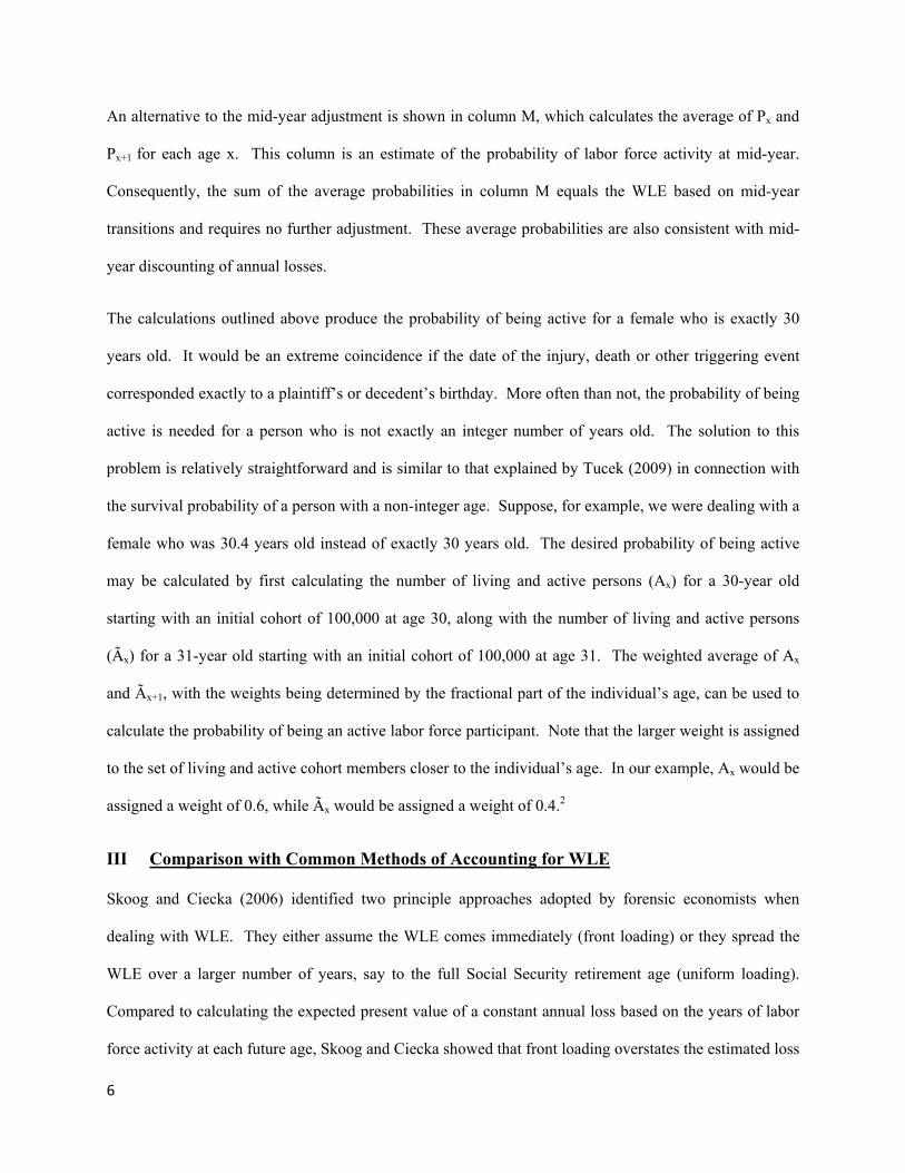
An alternative to the mid-year adjustment is shown in column M, which calculates the average of Px and

Px+1 for each age x. This column is an estimate of the probability of labor force activity at mid-year.

Consequently, the sum of the average probabilities in column M equals the WLE based on mid-year

transitions and requires no further adjustment. These average probabilities are also consistent with mid-

year discounting of annual losses.

The calculations outlined above produce the probability of being active for a female who is exactly 30

years old. It would be an extreme coincidence if the date of the injury, death or other triggering event

corresponded exactly to a plaintiff’s or decedent’s birthday. More often than not, the probability of being

active is needed for a person who is not exactly an integer number of years old. The solution to this

problem is relatively straightforward and is similar to that explained by Tucek (2009) in connection with

the survival probability of a person with a non-integer age. Suppose, for example, we were dealing with a

female who was 30.4 years old instead of exactly 30 years old. The desired probability of being active

may be calculated by first calculating the number of living and active persons (Ax) for a 30-year old

starting with an initial cohort of 100,000 at age 30, along with the number of living and active persons

(Ãx) for a 31-year old starting with an initial cohort of 100,000 at age 31. The weighted average of Ax

and Ãx+1, with the weights being determined by the fractional part of the individual’s age, can be used to

calculate the probability of being an active labor force participant. Note that the larger weight is assigned

to the set of living and active cohort members closer to the individual’s age. In our example, Ax would be

assigned a weight of 0.6, while Ãx would be assigned a weight of 0.4.2

III Comparison with Common Methods of Accounting for WLE

Skoog and Ciecka (2006) identified two principle approaches adopted by forensic economists when

dealing with WLE. They either assume the WLE comes immediately (front loading) or they spread the

WLE over a larger number of years, say to the full Social Security retirement age (uniform loading).

Compared to calculating the expected present value of a constant annual loss based on the years of labor

force activity at each future age, Skoog and Ciecka showed that front loading overstates the estimated loss

7  

for a variety of (positive) net discount rates. Similarly, they showed that uniform loading sometimes

overstates and sometimes understates the expected present value of the lost earnings. A variation of front

loading is to present the loss estimates with certainty for several years beyond WLE, ostensibly to give

the jury the latitude to decide whether the plaintiff would have been an active labor force participant for

fewer or more years than WLE suggests. This is characterized as the “WLE plus N” variant of front

loading in the discussion below.

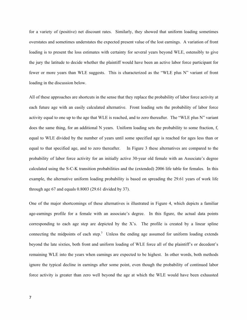
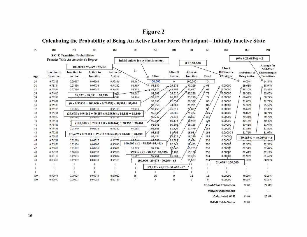
All of these approaches are shortcuts in the sense that they replace the probability of labor force activity at

each future age with an easily calculated alternative. Front loading sets the probability of labor force

activity equal to one up to the age that WLE is reached, and to zero thereafter. The “WLE plus N” variant

does the same thing, for an additional N years. Uniform loading sets the probability to some fraction, f,

equal to WLE divided by the number of years until some specified age is reached for ages less than or

equal to that specified age, and to zero thereafter. In Figure 3 these alternatives are compared to the

probability of labor force activity for an initially active 30-year old female with an Associate’s degree

calculated using the S-C-K transition probabilities and the (extended) 2006 life table for females. In this

example, the alternative uniform loading probability is based on spreading the 29.61 years of work life

through age 67 and equals 0.8003 (29.61 divided by 37).

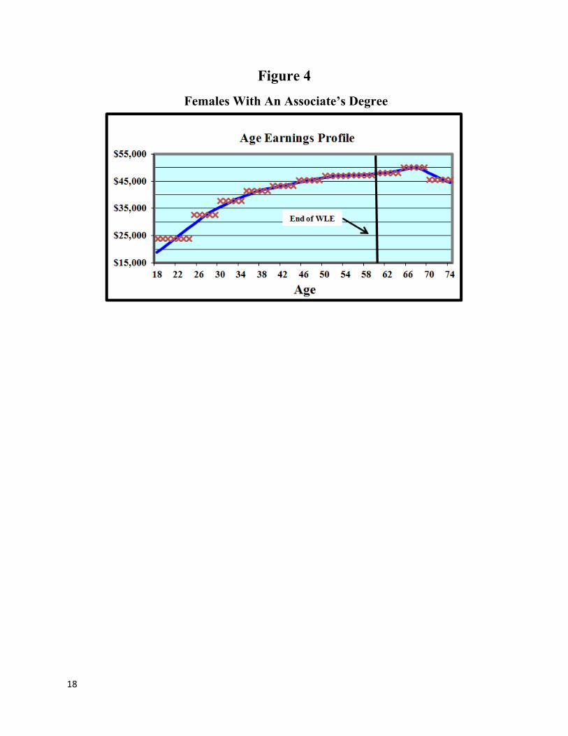
One of the major shortcomings of these alternatives is illustrated in Figure 4, which depicts a familiar

age-earnings profile for a female with an associate’s degree. In this figure, the actual data points

corresponding to each age step are depicted by the X’s. The profile is created by a linear spline

connecting the midpoints of each step.3 Unless the ending age assumed for uniform loading extends

beyond the late sixties, both front and uniform loading of WLE force all of the plaintiff’s or decedent’s

remaining WLE into the years when earnings are expected to be highest. In other words, both methods

ignore the typical decline in earnings after some point, even though the probability of continued labor

force activity is greater than zero well beyond the age at which the WLE would have been exhausted

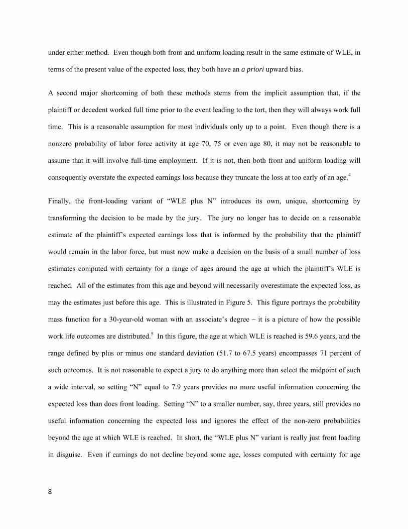
8  

under either method. Even though both front and uniform loading result in the same estimate of WLE, in

terms of the present value of the expected loss, they both have an a priori upward bias.

A second major shortcoming of both these methods stems from the implicit assumption that, if the

plaintiff or decedent worked full time prior to the event leading to the tort, then they will always work full

time. This is a reasonable assumption for most individuals only up to a point. Even though there is a

nonzero probability of labor force activity at age 70, 75 or even age 80, it may not be reasonable to

assume that it will involve full-time employment. If it is not, then both front and uniform loading will

consequently overstate the expected earnings loss because they truncate the loss at too early of an age.4

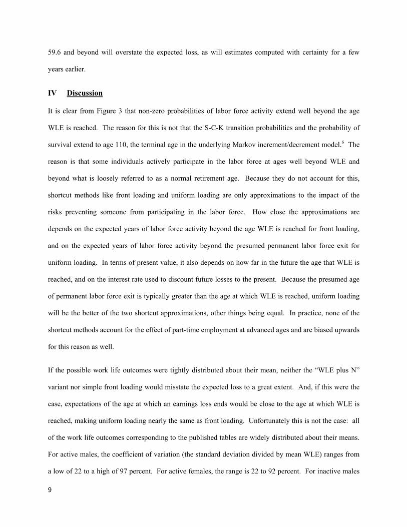
Finally, the front-loading variant of “WLE plus N” introduces its own, unique, shortcoming by

transforming the decision to be made by the jury. The jury no longer has to decide on a reasonable

estimate of the plaintiff’s expected earnings loss that is informed by the probability that the plaintiff

would remain in the labor force, but must now make a decision on the basis of a small number of loss

estimates computed with certainty for a range of ages around the age at which the plaintiff’s WLE is

reached. All of the estimates from this age and beyond will necessarily overestimate the expected loss, as

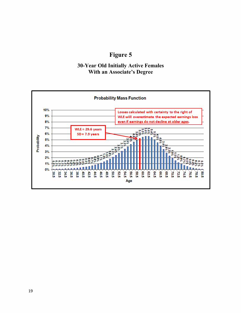
may the estimates just before this age. This is illustrated in Figure 5. This figure portrays the probability

mass function for a 30-year-old woman with an associate’s degree – it is a picture of how the possible

work life outcomes are distributed.5 In this figure, the age at which WLE is reached is 59.6 years, and the

range defined by plus or minus one standard deviation (51.7 to 67.5 years) encompasses 71 percent of

such outcomes. It is not reasonable to expect a jury to do anything more than select the midpoint of such

a wide interval, so setting “N” equal to 7.9 years provides no more useful information concerning the

expected loss than does front loading. Setting “N” to a smaller number, say, three years, still provides no

useful information concerning the expected loss and ignores the effect of the non-zero probabilities

beyond the age at which WLE is reached. In short, the “WLE plus N” variant is really just front loading

in disguise. Even if earnings do not decline beyond some age, losses computed with certainty for age

9  

59.6 and beyond will overstate the expected loss, as will estimates computed with certainty for a few

years earlier.

IV Discussion

It is clear from Figure 3 that non-zero probabilities of labor force activity extend well beyond the age

WLE is reached. The reason for this is not that the S-C-K transition probabilities and the probability of

survival extend to age 110, the terminal age in the underlying Markov increment/decrement model.6 The

reason is that some individuals actively participate in the labor force at ages well beyond WLE and

beyond what is loosely referred to as a normal retirement age. Because they do not account for this,

shortcut methods like front loading and uniform loading are only approximations to the impact of the

risks preventing someone from participating in the labor force. How close the approximations are

depends on the expected years of labor force activity beyond the age WLE is reached for front loading,

and on the expected years of labor force activity beyond the presumed permanent labor force exit for

uniform loading. In terms of present value, it also depends on how far in the future the age that WLE is

reached, and on the interest rate used to discount future losses to the present. Because the presumed age

of permanent labor force exit is typically greater than the age at which WLE is reached, uniform loading

will be the better of the two shortcut approximations, other things being equal. In practice, none of the

shortcut methods account for the effect of part-time employment at advanced ages and are biased upwards

for this reason as well.

If the possible work life outcomes were tightly distributed about their mean, neither the “WLE plus N”

variant nor simple front loading would misstate the expected loss to a great extent. And, if this were the

case, expectations of the age at which an earnings loss ends would be close to the age at which WLE is

reached, making uniform loading nearly the same as front loading. Unfortunately this is not the case: all

of the work life outcomes corresponding to the published tables are widely distributed about their means.

For active males, the coefficient of variation (the standard deviation divided by mean WLE) ranges from

a low of 22 to a high of 97 percent. For active females, the range is 22 to 92 percent. For inactive males

10  

and females the ranges are 23 to 359 percent and 23 to 486 percent. Although the variation in the

distribution of work life outcomes increases in relative terms for both males and females as age increases,

it decreases in absolute terms. However, the standard error falls below 3 years only at very late ages – no

earlier than age 62 for males (initially inactive with no diploma or GED) and 58 for females (initially

inactive with no diploma or GED). Thus, the instances in which arbitrarily setting “N” to a low number

might result in a range of at least plus or minus one standard deviation are limited to older plaintiffs and

decedents.

Compared to any of the shortcut methods, explicit calculation of the probability of labor force activity

offers several advantages. First, and most important, there is no a priori bias in the resulting estimate of

the expected loss because it estimates the expected loss directly and accounts for the wide variation in

work life outcomes. Second, explicit calculation of the probability of labor force activity allows one to

use updated mortality tables and to account for the implicit assumption that an injured plaintiff will be

alive on the date of the trial.

A third advantage arises in cases where a loss is contingent upon the survival of a plaintiff who is not the

injured person or decedent – financial support or medical insurance provided to a spouse are examples.

The expected present value of such losses necessarily depends on the survival probability of the non-

injured plaintiff. And, if the loss is also contingent on the employment of the injured person, explicit use

of the probability of labor force activity in lieu of front or uniform loading provides a consistent means of

accounting for the risk that the loss component may not have been realized even if the event leading to the

tort had not occurred.7

Finally, explicit calculation of the probability of labor force activity allows consideration of part-time

employment at older ages and does not force all of the labor force activity into earlier, higher income

years.

11  

Nevertheless, there are drawbacks to using the probability of labor force activity in lieu of any of the three

shortcut methods. For one thing, the required calculations are necessarily more complex. Additionally,

using the full range of the probability of labor force activity requires an estimate of earnings for years

beyond age 70.

Even though the calculations are more complex than those required by any of the shortcut methods, they

are within the reach of any competent forensic economist and can easily be performed using an Excel

spreadsheet or other application. More important, just because the calculations are complex doesn’t mean

that the explanation has to be. To object to use of the probability of labor force activity because of

complexity is to abdicate one’s role as an expert: if use of only simple calculations were a requirement

for loss estimates, then the courts would have little need for economic experts. It is clearly not necessary

to explain how the probability of labor force activity is calculated, just as it is not necessary to explain

how present values or survival probabilities are calculated. It is sufficient only to explain that the

underlying calculations take into account that the plaintiff may die, may become injured or sick, or may

not be an active labor force participant for any other reason. In short, the same explanation as is given for

WLE will suffice.

The need to estimate annual earnings for years beyond age 70 is a more substantive drawback. While use

of an age-earnings profile may capture an expected decline in full-time earnings at older ages, it will not

necessarily reflect the decrease due to part-time employment.8 The real issue, however, is whether

assuming, as the alternative approaches do, that earnings equal zero once a certain age is reached is more

reasonable than presenting earnings assumptions that cover the full range of the probability of labor force

activity. It is possible to make reasonable assumptions about earnings beyond WLE or some assumed

retirement age, and to present the loss estimates in such a way that the jurors can adjust them as they

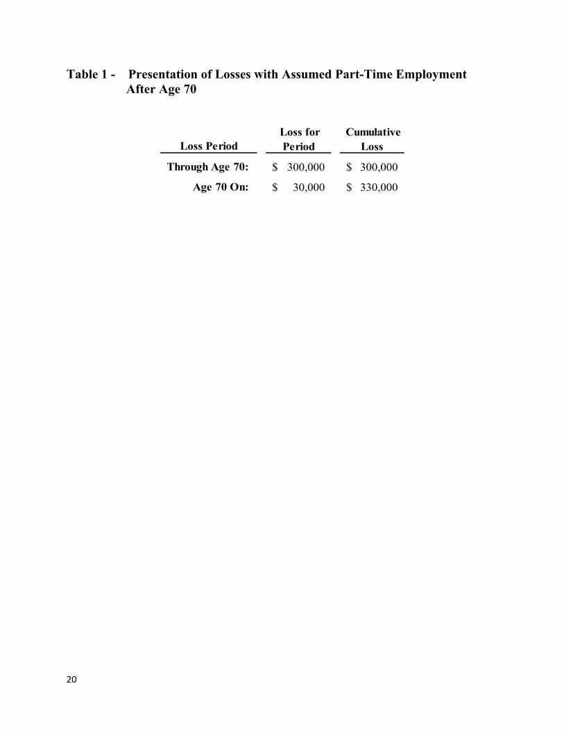
believe best, based on the specifics of the case. Table 1 presents an example of how this may be done. In

this example, it is assumed that part-time employment at half the full-time earnings starts at age 70. If the

jurors believe that the part-time earnings would be only one-fourth the full-time level, it is easy to explain

12  

that they need only subtract half of the $30,000 from the total to arrive at a total loss of $315,000.

Similarly, if they believe earnings will always be at the full-time level, it is easy to explain that they need

only add $30,000 to the total.

V Conclusions

This paper has presented the calculations needed to compute the probability of labor force activity for a

person who is an initially active or an initially inactive labor force participant using the S-C-K transition

probabilities. Three alternatives to the explicit use of the probability of labor force activity to estimate an

expected earnings loss were identified: (1) front loading; (2) uniform loading; and (3) the WLE plus N

variant of front loading. As shown in Figure 3, each of these alternatives replaces the probability of labor

force activity at each future age with an easily calculated substitute. These substitutes shift the

probability of labor force activity to younger ages and set it to zero at some point even though the S-C-K

transition probabilities produce greater-than-zero probabilities of labor force activity at ages beyond this

point. This shifting creates an a priori bias in each of the shortcut alternatives by forcing all of the

remaining labor force activity into the years when earnings can be expected to be highest and by ignoring

a decline in earnings at later ages due to age-profile effects or to a shift to part-time employment. The

wide variation in work life outcomes makes the shortcut alternatives less attractive than explicit reliance

on the probability of labor force activity to estimate the expected earnings loss.

Explicit use of the probability of labor force activity offers several advantages: (1) it does not suffer from

the a priori bias of the shortcut methods; (2) it allows one to use the most recent mortality tables and to

explicitly account for the assumption that an injured plaintiff is alive on the date of the trial; (3) it permits

consistent treatment of mortality risk when losses are incurred by non-injured plaintiffs; and (4) it does

not ignore the decline in earnings due to age-profile effects or to a shift to part-time employment.

There are drawbacks to the explicit use of the probability of labor force activity: the approach is more

complex and it requires earnings estimates at age 70 and beyond. The first drawback is easily overcome,

13  

since the required calculations are within the reach of any competent forensic economist and since

complex calculations do not necessitate complex explanations. The second drawback is more

problematic, but can be overcome by presenting losses in the fashion illustrated in Table 1.

On balance, even though using the probability of labor force activity in lieu of other commonly-used

alternatives requires a bit more explaining and a somewhat more detailed presentation of the loss

estimates, the advantages seem to overcome the drawbacks. No one can say for certain what a plaintiff’s

future earnings would have been but for his injury. At best, a forensic economist can only estimate the

expected loss. Because the alternative approaches move the loss earlier in time, and because earnings at

ages beyond what is considered to be normal retirement may be lower, the alternatives have an a priori

bias in favor of overstating the expected loss. At bottom, the fact that other means of accounting for

WLE ignore the underlying probability distribution, as well as the possibility that earnings in the years

beyond the age WLE is reached may very well be at a lower level, carries the decision in favor of fully

utilizing the S-C-K transition probabilities as explained above.

14  

References

Arias, Elizabeth, “United States Life Tables, 2006”, National Vital Statistics Report, 58(21), 2010, pp. 1-

40, National Center for Health Statistics. Skoog, Gary R., James E. Ciecka and Kurt V. Krueger,  "The Markov Process Model of Labor Force

Activity: Extended Tables of Central Tendency, Shape, Percentile Points, and Bootstrap Standard Errors", Journal of Forensic Economics, 22(2), 2011, pp.165-229.

_____, James E. Ciecka, “Allocation of Worklife Expectancy and the Analysis of Front and Uniform

Loading with Nomograms”, Journal of Forensic Economics, 19(3), 2006, pp. 261-296). Slesnick, Frank T., Michael R. Luthy, and Michael L. Brookshire, “A 2012 Survey of Forensic

Economists: Their Methods, Estimates and Perspectives”, Journal of Forensic Economics, 24(1), 2013, pp.67-99.

Tucek, David G., “Calculating Survival Probabilities”, Journal of Legal Economics, 2009, Vol. 16(1), pp.

111-126.

15  

Figure 1

Calculating the Probability of Being An Active Labor Force Participant – Initially Active State

16  

Figure 2

Calculating the Probability of Being An Active Labor Force Participant – Initially Inactive State

17  

Figure 3

Front and Uniform Loading Compared to Probability of Being an Active Labor Force Participant

WLE plus N 

18  

Figure 4

Females With An Associate’s Degree

19  

Figure 5

30-Year Old Initially Active Females With an Associate’s Degree

20  

Table 1 - Presentation of Losses with Assumed Part-Time Employment After Age 70

Through Age 70: 300,000$ 300,000$

Age 70 On: 30,000$ 330,000$

Loss for Period

Cumulative Loss Loss Period

21  

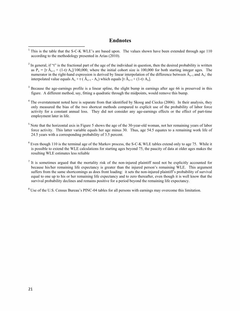
Endnotes                                                             1 This is the table that the S-C-K WLE’s are based upon. The values shown have been extended through age 110

according to the methodology presented in Arias (2010).  2 In general, if “t” is the fractional part of the age of the individual in question, then the desired probability is written

as Px = [t·Ãx+1 + (1-t)·Ax]/100,000, where the initial cohort size is 100,000 for both starting integer ages. The numerator in the right-hand expression is derived by linear interpolation of the difference between Ãx+1 and Ax: the interpolated value equals Ax + t·( Ãx+1 - Ax) which equals [t·Ãx+1 + (1-t)·Ax]. 

 3 Because the age-earnings profile is a linear spline, the slight bump in earnings after age 66 is preserved in this

figure. A different method, say, fitting a quadratic through the midpoints, would remove this bump. 4 The overstatement noted here is separate from that identified by Skoog and Ciecka (2006). In their analysis, they

only measured the bias of the two shortcut methods compared to explicit use of the probability of labor force activity for a constant annual loss. They did not consider any age-earnings effects or the effect of part-time employment later in life.

 5 Note that the horizontal axis in Figure 5 shows the age of the 30-year-old woman, not her remaining years of labor

force activity. This latter variable equals her age minus 30. Thus, age 54.5 equates to a remaining work life of 24.5 years with a corresponding probability of 3.5 percent.

 6 Even though 110 is the terminal age of the Markov process, the S-C-K WLE tables extend only to age 75. While it

is possible to extend the WLE calculations for starting ages beyond 75, the paucity of data at older ages makes the resulting WLE estimates less reliable

 7  It is sometimes argued that the mortality risk of the non-injured plaintiff need not be explicitly accounted for

because his/her remaining life expectancy is greater than the injured person’s remaining WLE. This argument suffers from the same shortcomings as does front loading: it sets the non-injured plaintiff’s probability of survival equal to one up to his or her remaining life expectancy and to zero thereafter, even though it is well know that the survival probability declines and remains positive for a period beyond the remaining life expectancy. 

 8 Use of the U.S. Census Bureau’s PINC-04 tables for all persons with earnings may overcome this limitation.