95 [ Journal of Labor Economics, 2007, vol. 25, no. 1] 2007 by The University of Chicago. All rights reserved. 0734-306X/2007/2501-0004$10.00 Teachers and Student Achievement in the Chicago Public High Schools Daniel Aaronson, Federal Reserve Bank of Chicago Lisa Barrow, Federal Reserve Bank of Chicago William Sander, DePaul University We estimate the importance of teachers in Chicago public high schools using matched student-teacher administrative data. A one standard deviation, one semester improvement in math teacher qual- ity raises student math scores by 0.13 grade equivalents or, over 1 year, roughly one-fifth of average yearly gains. Estimates are rela- tively stable over time, reasonably impervious to a variety of con- ditioning variables, and do not appear to be driven by classroom sorting or selective score reporting. Also, teacher quality is partic- ularly important for lower-ability students. Finally, traditionalhuman capital measures—including those determining compensation—ex- plain little of the variation in estimated quality. We thank the Chicago Public Schools and the Consortium on Chicago School Research at the University of Chicago for making the data available to us. We are particularly grateful to John Easton and Jenny Nagaoka for their help in putting together the data and answering our many follow-up questions. We thank Joe Altonji, Kristin Butcher, Dave Card, Rajeev Dehejia, Tom DiCiccio, Eric French, Brian Jacob, Jeff Kling, Steve Rivkin, Doug Staiger, Dan Sullivan, Chris Taber, and seminar participants at many universities and conferences for helpful comments and discussions. The views expressed in this article are ours and are not necessarily those of the Federal Reserve Bank of Chicago or the Federal Reserve System. Contact the corresponding author, Lisa Barrow, at lbarrow@ frbchi.org.

Welcome message from author
This document is posted to help you gain knowledge. Please leave a comment to let me know what you think about it! Share it to your friends and learn new things together.
Transcript

95
[ Journal of Labor Economics, 2007, vol. 25, no. 1]� 2007 by The University of Chicago. All rights reserved.0734-306X/2007/2501-0004$10.00
Teachers and Student Achievement inthe Chicago Public High Schools
Daniel Aaronson, Federal Reserve Bank of Chicago
Lisa Barrow, Federal Reserve Bank of Chicago
William Sander, DePaul University
We estimate the importance of teachers in Chicago public highschools using matched student-teacher administrative data. A onestandard deviation, one semester improvement in math teacher qual-ity raises student math scores by 0.13 grade equivalents or, over 1year, roughly one-fifth of average yearly gains. Estimates are rela-tively stable over time, reasonably impervious to a variety of con-ditioning variables, and do not appear to be driven by classroomsorting or selective score reporting. Also, teacher quality is partic-ularly important for lower-ability students. Finally, traditional humancapital measures—including those determining compensation—ex-plain little of the variation in estimated quality.
We thank the Chicago Public Schools and the Consortium on Chicago SchoolResearch at the University of Chicago for making the data available to us. Weare particularly grateful to John Easton and Jenny Nagaoka for their help inputting together the data and answering our many follow-up questions. We thankJoe Altonji, Kristin Butcher, Dave Card, Rajeev Dehejia, Tom DiCiccio, EricFrench, Brian Jacob, Jeff Kling, Steve Rivkin, Doug Staiger, Dan Sullivan, ChrisTaber, and seminar participants at many universities and conferences for helpfulcomments and discussions. The views expressed in this article are ours and arenot necessarily those of the Federal Reserve Bank of Chicago or the FederalReserve System. Contact the corresponding author, Lisa Barrow, at [email protected].
96 Aaronson et al.
I. Introduction
The Coleman Report (Coleman et al. 1966) broke new ground in theestimation of education production functions, concluding that familybackground and peers were more important than schools and teachers ineducational outcomes such as test scores and graduation rates. While re-search since Coleman supports the influence of family background, sub-stantiation of the importance of other factors, particularly schools andteachers, has evolved slowly with the release of better data. Today, mostresearchers agree that schools and teachers matter.1 However, how muchthey matter, the degree to which they vary across subpopulations, howrobust quality rankings are to specification choices, and whether mea-surable characteristics such as teacher education and experience affectstudent educational outcomes continue to be of considerable research andpolicy interest.
In this study, we use administrative data from the Chicago public highschools to estimate the importance of teachers on student mathematicstest score gains and then relate our measures of individual teacher effec-tiveness to observable characteristics of the instructors. Our measure ofteacher quality is the effect on ninth-grade math scores of a semester ofinstruction with a given teacher, controlling for eighth-grade math scoresand student characteristics. Our data provide us with a key advantage ingenerating this estimate: the ability to link teachers and students in specificclassrooms. In contrast, many other studies can only match students tothe average teacher in a grade or school. In addition, because teachers areobserved in multiple classroom settings, our teacher effect estimates areless likely to be driven by idiosyncratic class effects. Finally, the admin-istrative teacher records allow us to separate the effects of observed teachercharacteristics from unobserved aspects of teacher quality.
Consistent with earlier studies, we find that teachers are importantinputs in ninth-grade math achievement. Namely, after controlling forinitial ability (as measured by test scores) and other student characteristics,teacher effects are statistically important in explaining ninth-grade mathtest score achievement, and the variation in teacher effect estimates is large
1 Literature reviews include Greenwald, Hedges, and Laine (1996) and Hanu-shek (1996, 1997, 2002). A brief sampling of other work on teacher effects includesMurnane (1975), Goldhaber and Brewer (1997), Angrist and Lavy (2001), Jepsenand Rivkin (2002), Rivers and Sanders (2002), Jacob and Lefgren (2004), Rockoff(2004), Kane and Staiger (2005), Rivkin, Hanushek, and Kain (2005), and Kane,Rockoff, and Staiger (2006). The earliest studies on teacher quality were hamperedby data availability and thus often relied on state- or school-level variation. Ag-gregation and measurement error compounded by proxies such as student-teacherratios and average teacher experience can introduce significant bias. More recentstudies, such as Rockoff (2004), Kane and Staiger (2005), Rivkin et al. (2005), andKane et al. (2006), use administrative data like ours to minimize these concerns.
Teachers and Student Achievement 97
enough such that the expected difference in math achievement betweenhaving an average teacher and one that is one standard deviation aboveaverage is educationally important. However, a certain degree of cautionmust be exercised in estimating teacher quality using teacher fixed effectsas biases related to measurement, particularly due to small populationsof students used to identify certain teachers, can critically influence results.Sampling variation overstates our measures of teacher quality dispersionby amounts roughly similar to Kane and Staiger’s (2002, 2005) evaluationsof North Carolina schools and Los Angeles teachers. Correcting for sam-pling error, we find that the standard deviation in teacher quality in theChicago public high schools is at least 0.13 grade equivalents per semester.Thus, over two semesters, a one standard deviation improvement in mathteacher quality translates into an increase in math achievement equal to22% of the average annual gain. This estimate is a bit higher than, butstatistically indistinguishable from, those reported in Rockoff (2004) andRivkin et al. (2005).2
Furthermore, we show that our results are unlikely to be driven byclassroom sorting or selective use of test scores and, perhaps most im-portantly, the individual teacher ratings are relatively stable over time andreasonably impervious to a wide variety of conditioning variables. Thelatter result suggests that test score value-added measures for teacher pro-ductivity are not overly sensitive to reasonable statistical modeling de-cisions, and thus incentive schemes in teacher accountability systems thatrely on similar estimates of productivity are not necessarily weakened bylarge measurement error in teacher productivity.
We also show how estimates vary by initial (eighth-grade) test scores,race, and sex and find that the biggest impact of a higher quality teacher,relative to the mean gain of that group, is among African American stu-dents and those with low or middle range eighth-grade test scores. Wefind no difference between boys and girls.
Finally, the vast majority of the variation in teacher effects is unex-plained by easily observable teacher characteristics, including those usedfor compensation. While some teacher attributes are consistently relatedto our quality measure, together they explain at most 10% of the totalvariation in estimated teacher quality. Most troubling, the variables thatdetermine compensation in Chicago—tenure, advanced degrees, andteaching certifications—explain roughly 1% of the total variation in es-
2 Rivkin et al.’s (2005) lower bound estimates suggest that a one standard de-viation increase in teacher quality increases student achievement by at least 0.11standard deviations. Rockoff (2004) reports a 0.1 standard deviation gain from aone standard deviation increase in teacher quality from two New Jersey suburbanschool districts. In our results, a one standard deviation increase in teacher qualityover a full year implies about a 0.15 standard deviation increase in math test scoregains.
98 Aaronson et al.
timated teacher quality. These results highlight the lack of a close rela-tionship between teacher pay and productivity and the difficulty in de-veloping compensation schedules that reward teachers for good workbased solely on certifications, degrees, and other standard administrativedata. That is not to say such schemes are not viable. Here, the economicallyand statistically important persistence of teacher quality over time shouldbe underscored. By using past performance, administrators can predictteacher quality. Of course, such a history might not exist when recruiting,especially for rookie teachers, or may be overwhelmed by sampling var-iation for new hires, a key hurdle in prescribing recruitment, retention,and compensation strategies at the beginning of the work cycle. Never-theless, there is clearly scope for using test score data among other eval-uation tools for tenure, compensation, and classroom organization deci-sions.
While our study focuses on only one school district over a 3-yearperiod, this district serves a large population of minority and lower incomestudents, typical of many large urban districts in the United States. Fifty-five percent of ninth graders in the Chicago public schools are AfricanAmerican, 31% are Hispanic, and roughly 80% are eligible for free orreduced-price school lunch. Similarly, New York City, Los Angeles Uni-fied, Houston Independent School District, and Philadelphia City servestudent populations that are 80%–90% nonwhite and roughly 70%–80%eligible for free or reduced-price school lunch (U.S. Department of Ed-ucation 2003). Therefore, on these dimensions Chicago is quite represen-tative of the school systems that generate the most concern in educationpolicy discussions.
II. Background and Data
The unique detail and scope of our data are major strengths of thisstudy. Upon agreement with the Chicago Public Schools (CPS), the Con-sortium on Chicago School Research at the University of Chicago pro-vided us with administrative records from the city’s public high schools.These records include all students enrolled and teachers working in 88CPS high schools from 1996–97 to 1998–99.3 We concentrate on the per-formance of ninth graders in this article.
The key advantage to using administrative records is being able to workwith the population of students, a trait of several other recent studies,including Rockoff (2004), Kane and Staiger (2005), Rivkin et al. (2005),and Kane et al. (2006). Apart from offering a large sample of urban school-children, the CPS administrative records provide several other useful fea-
3 Of the 88 schools, six are so small that they do not meet criteria on samplesizes that we describe below. These schools are generally more specialized, servingstudents who have not succeeded in the regular school programs.
Teachers and Student Achievement 99
tures that rarely appear together in other studies. First, this is the firststudy that we are aware of that examines high school teachers. Clearly,it is important to understand teacher effects at all points in the educationprocess. Studying high schools has the additional advantage that class-rooms are subject specific, and our data provide enough school schedulingdetail to construct actual classrooms. Thus, we can examine student-teacher matches at a level that plausibly corresponds with what we thinkof as a teacher effect. This allows us to isolate the impact of math teacherson math achievement gains. However, we can go even further by, say,looking at the impact of English teachers on math gains. In this study,we report such exercises as robustness checks, but data like these offersome potential for exploring externalities or complementarities betweenteachers.
The teacher records also include specifics about human capital anddemographics. These data allow us to decompose the teacher effect var-iation into shares driven by unobservable and observable factors, includingthose on which compensation is based. Finally, the student and teacherrecords are longitudinal. This has several advantages. Although our dataare limited to high school students, they include a history of pre–highschool test scores that can be used as controls for past (latent) inputs.Furthermore, each teacher is evaluated based on multiple classrooms over(potentially) multiple years, thus mitigating the influence of unobservedidiosyncratic class effects.
A. Student Records
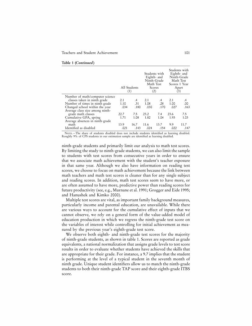
There are three general components of the student data: test scores,school and scheduling variables, and family and student background mea-sures. Like most administrative data sets, the latter is somewhat limited.Table 1 includes descriptive statistics for some of the variables available,including sex, race, age, eligibility for the free or reduced school lunchprogram, and guardian (mom, dad, grandparent, etc.). Residential locationis also provided, allowing us to incorporate census tract information oneducation, income, and house values. We concentrate our discussion belowon the test score and scheduling measures that are less standard.
1. Test Scores
In order to measure student achievement, we rely on student test scoresfrom two standardized tests administered by the Chicago PublicSchools—the Iowa Test of Basic Skills (ITBS) administered in the springof grades 3–8 and the Test of Achievement and Proficiency (TAP) ad-ministered during the spring for grades 9 and 11.4 We limit the study to
4 TAP testing was mandatory for grades 9 and 11 through 1998. The year 1999was a transition year in which ninth, tenth, and eleventh graders were tested.Starting in 2000, TAP testing is mandatory for grades 9 and 10.
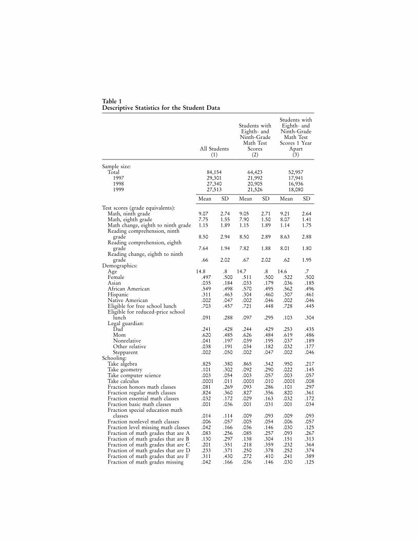
Table 1Descriptive Statistics for the Student Data
All Students(1)
Students withEighth- andNinth-Grade
Math TestScores
(2)
Students withEighth- andNinth-Grade
Math TestScores 1 Year
Apart(3)
Sample size:Total 84,154 64,423 52,957
1997 29,301 21,992 17,9411998 27,340 20,905 16,9361999 27,513 21,526 18,080
Mean SD Mean SD Mean SD
Test scores (grade equivalents):Math, ninth grade 9.07 2.74 9.05 2.71 9.21 2.64Math, eighth grade 7.75 1.55 7.90 1.50 8.07 1.41Math change, eighth to ninth grade 1.15 1.89 1.15 1.89 1.14 1.75Reading comprehension, ninth
grade 8.50 2.94 8.50 2.89 8.63 2.88Reading comprehension, eighth
grade 7.64 1.94 7.82 1.88 8.01 1.80Reading change, eighth to ninth
grade .66 2.02 .67 2.02 .62 1.95Demographics:
Age 14.8 .8 14.7 .8 14.6 .7Female .497 .500 .511 .500 .522 .500Asian .035 .184 .033 .179 .036 .185African American .549 .498 .570 .495 .562 .496Hispanic .311 .463 .304 .460 .307 .461Native American .002 .047 .002 .046 .002 .046Eligible for free school lunch .703 .457 .721 .448 .728 .445Eligible for reduced-price school
lunch .091 .288 .097 .295 .103 .304Legal guardian:
Dad .241 .428 .244 .429 .253 .435Mom .620 .485 .626 .484 .619 .486Nonrelative .041 .197 .039 .195 .037 .189Other relative .038 .191 .034 .182 .032 .177Stepparent .002 .050 .002 .047 .002 .046
Schooling:Take algebra .825 .380 .865 .342 .950 .217Take geometry .101 .302 .092 .290 .022 .145Take computer science .003 .054 .003 .057 .003 .057Take calculus .0001 .011 .0001 .010 .0001 .008Fraction honors math classes .081 .269 .093 .286 .101 .297Fraction regular math classes .824 .360 .827 .356 .820 .361Fraction essential math classes .032 .172 .029 .163 .032 .172Fraction basic math classes .001 .036 .001 .031 .001 .034Fraction special education math
classes .014 .114 .009 .093 .009 .093Fraction nonlevel math classes .006 .057 .005 .054 .006 .057Fraction level missing math classes .042 .166 .036 .146 .030 .125Fraction of math grades that are A .083 .256 .085 .257 .093 .267Fraction of math grades that are B .130 .297 .138 .304 .151 .313Fraction of math grades that are C .201 .351 .218 .359 .232 .364Fraction of math grades that are D .233 .371 .250 .378 .252 .374Fraction of math grades that are F .311 .430 .272 .410 .241 .389Fraction of math grades missing .042 .166 .036 .146 .030 .125
Teachers and Student Achievement 101
Table 1 (Continued)
All Students(1)
Students withEighth- andNinth-Grade
Math TestScores
(2)
Students withEighth- andNinth-Grade
Math TestScores 1 Year
Apart(3)
Number of math/computer scienceclasses taken in ninth grade 2.1 .4 2.1 .4 2.1 .4
Number of times in ninth grade 1.10 .31 1.08 .28 1.00 .00Changed school within the year .034 .180 .030 .170 .027 .163Average class size among ninth-
grade math classes 22.7 7.5 23.2 7.4 23.6 7.5Cumulative GPA, spring 1.71 1.08 1.82 1.04 1.93 1.03Average absences in ninth-grade
math 13.9 16.7 11.6 13.7 9.9 11.7Identified as disabled .021 .143 .024 .154 .022 .147
Note.—The share of students disabled does not include students identified as learning disabled.Roughly 9% of CPS students in our estimation sample are identified as learning disabled.
ninth-grade students and primarily limit our analysis to math test scores.By limiting the study to ninth-grade students, we can also limit the sampleto students with test scores from consecutive years in order to ensurethat we associate math achievement with the student’s teacher exposurein that same year. Although we also have information on reading testscores, we choose to focus on math achievement because the link betweenmath teachers and math test scores is cleaner than for any single subjectand reading scores. In addition, math test scores seem to have more, orare often assumed to have more, predictive power than reading scores forfuture productivity (see, e.g., Murnane et al. 1991; Grogger and Eide 1995;and Hanushek and Kimko 2000).
Multiple test scores are vital, as important family background measures,particularly income and parental education, are unavailable. While thereare various ways to account for the cumulative effect of inputs that wecannot observe, we rely on a general form of the value-added model ofeducation production in which we regress the ninth-grade test score onthe variables of interest while controlling for initial achievement as mea-sured by the previous year’s eighth-grade test score.
We observe both eighth- and ninth-grade test scores for the majorityof ninth-grade students, as shown in table 1. Scores are reported as gradeequivalents, a national normalization that assigns grade levels to test scoreresults in order to evaluate whether students have achieved the skills thatare appropriate for their grade. For instance, a 9.7 implies that the studentis performing at the level of a typical student in the seventh month ofninth grade. Unique student identifiers allow us to match the ninth-gradestudents to both their ninth-grade TAP score and their eighth-grade ITBSscore.
102 Aaronson et al.
Eighth- and ninth-grade test score data are reported for between 75%and 78% of the ninth-grade students in the CPS, yielding a potentialsample of around 64,000 unique students over the 3-year period. Oursample drops to 53,000 when we exclude students without eighth- andninth-grade test scores in consecutive school years and those with testscore gains in the 1st and 99th percentiles.
Since the ninth-grade test is not a high stakes test for either studentsor teachers, it is less likely to elicit “cheating” in any form compared tothe explicit teacher cheating uncovered in Jacob and Levitt (2003). Inaddition, by eliminating the outlier observations in terms of test scoregains, we may drop some students for whom either the eighth- or ninth-grade test score is “too high” due to cheating. That said, there may bereasonable concern that missing test scores reflect some selection aboutwhich students take the tests or which test scores are reported.
Approximately 11% of ninth graders do not have an eighth-grade mathtest score, and 17% do not have a ninth-grade score.5 There are severalpossible explanations for this outcome: students might have transferredfrom another district, did not take the exam, or perhaps simply did nothave scores appearing in the database. Missing data appear more likelyfor the subset of students who tend to be male, white or Hispanic, older,and designated as having special education status (and thus potentiallyexempt from the test). Convincing exclusion restrictions are not availableto adequately assess the importance of selection of this type.6 However,later in the article we show that our quality measure is not correlatedwith missing test scores, suggesting that this type of selection or gamingof the system does not unduly influence our measure of teacher quality.
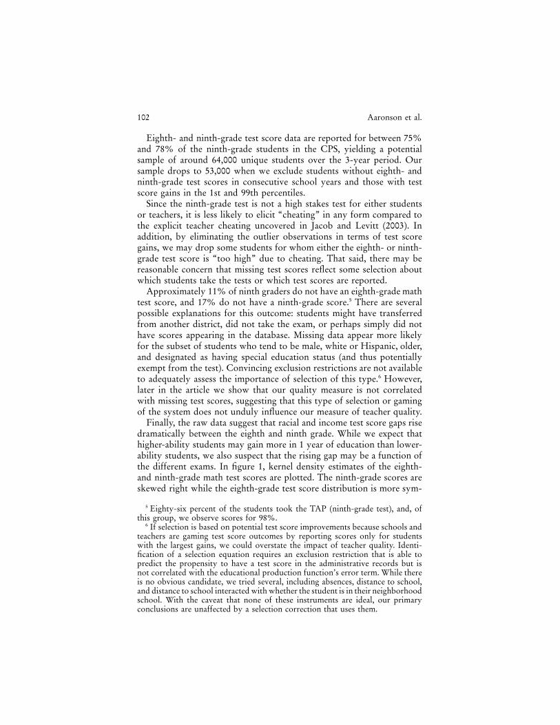
Finally, the raw data suggest that racial and income test score gaps risedramatically between the eighth and ninth grade. While we expect thathigher-ability students may gain more in 1 year of education than lower-ability students, we also suspect that the rising gap may be a function ofthe different exams. In figure 1, kernel density estimates of the eighth-and ninth-grade math test scores are plotted. The ninth-grade scores areskewed right while the eighth-grade test score distribution is more sym-
5 Eighty-six percent of the students took the TAP (ninth-grade test), and, ofthis group, we observe scores for 98%.
6 If selection is based on potential test score improvements because schools andteachers are gaming test score outcomes by reporting scores only for studentswith the largest gains, we could overstate the impact of teacher quality. Identi-fication of a selection equation requires an exclusion restriction that is able topredict the propensity to have a test score in the administrative records but isnot correlated with the educational production function’s error term. While thereis no obvious candidate, we tried several, including absences, distance to school,and distance to school interacted with whether the student is in their neighborhoodschool. With the caveat that none of these instruments are ideal, our primaryconclusions are unaffected by a selection correction that uses them.
Teachers and Student Achievement 103
Fig. 1.—Kernel density estimates of eighth- and ninth-grade math test scores. Test scoresare measured in grade equivalents. Estimates are calculated using the Epanechnikov kernel.For the eighth-grade test score a bin width of approximately 0.14 is used, while for theninth-grade test a bin width of approximately 0.26 is used.
metric. As a consequence, controlling for eighth-grade test scores in theregression of ninth-grade test scores on teacher indicators and other stu-dent characteristics may not adequately control for the initial quality ofa particular teacher’s students and may thus lead us to conclude thatteachers with better than average students are superior instructors. Wedrop the top and bottom 1% of the students by change in test scores topartly account for this problem. We also discuss additional strategies,including using alternative test score measures that are immune to dif-ferences in scaling of the test, accounting for student attributes, and an-alyzing groups of students by initial ability.
2. Classroom Scheduling
A second important feature of the student data is the detailed schedulinginformation that allows us to construct the complete history of a student’sclass schedule while in the CPS high schools. The data include where(room number) and when (semester and period) the class met, the teacherassigned, the title of the class, and the course level (i.e., advanced place-ment, regular, etc.). Furthermore, we know the letter grade received andthe number of classroom absences. Because teachers and students werematched to the same classroom, we have more power to estimate teacher
104 Aaronson et al.
effects than is commonly available in administrative records where match-ing occurs at the school or grade level. Additionally, since we have thisinformation for every student, we are able to calculate measures of class-room peers.
One natural concern in estimating teacher quality is whether there arelingering influences from the classroom sorting process. That is, studentsmay be purposely placed with certain instructors based on their learningpotential. The most likely scenario involves parental lobbying, which maybe correlated with expected test score gains, but a school or teacher mayalso exert influence that results in nonrandom sorting of students.7
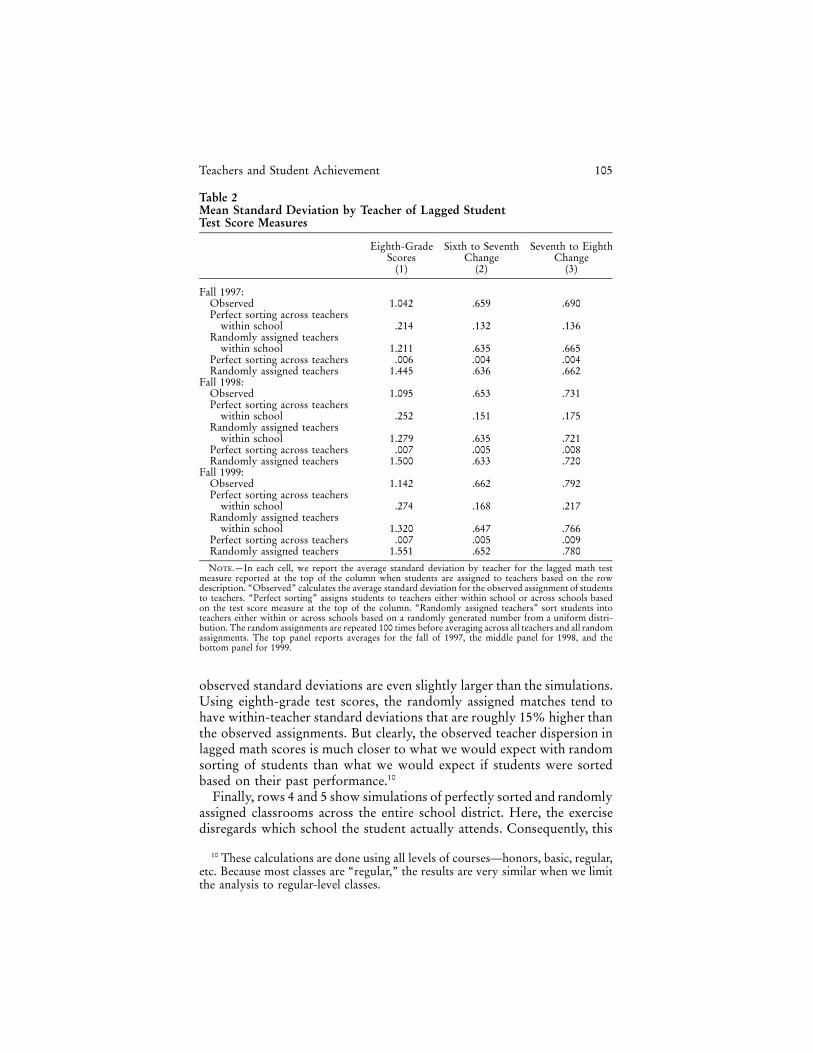
To assess the extent to which students may be sorted based on expectedtest score gains, we calculate test score dispersion for the observed teacherassignments and for several counterfactual teacher assignments. In table2, we report the degree to which the observed within-teacher standarddeviation in students’ pre-ninth-grade performance differs from simulatedclassrooms that are either assigned randomly or sorted based on test scorerank. We use three lagged test score measures for assignment: eighth-grade test scores, sixth- to seventh-grade test score gains, and seventh- toeighth-grade test score gains. Each panel reports results for the three fallsemesters in our data.8 The top row of each panel, labeled “Observed,”displays the observed average within-teacher standard deviation of thesemeasures. This is the baseline to which we compare the simulations. Eachof the four subsequent rows assigns students to teachers either randomlyor based on pre-ninth-grade performance.
Row 2 displays the average within-teacher standard deviation whenstudents are perfectly sorted across teachers within their home school.9
Such a within-school sorting mechanism reduces the within-teacher stan-dard deviation to roughly 20% of the observed analog. In contrast, if werandomly assign students to classrooms within their original school, asshown in row 3, the average within-teacher standard deviation is veryclose to the within-teacher standard deviation that is observed in the data.Strikingly, there is no evidence that sorting occurs on past gains; the
7 Informal discussions with a representative of the Chicago public school systemsuggest that parents have little influence on teacher selection and, conditional oncourse level, the process is not based on student characteristics. Moreover, ouruse of first-year high school students may alleviate concern since it is likely moredifficult for schools to evaluate new students, particularly on unobservablecharacteristics.
8 The estimates for the spring semester are very similar and available from theauthors on request.
9 For example, within an individual school, say there are three classrooms with15, 20, and 25 students. In the simulation, the top 25 students, based on our pre-ninth-grade measures, would be placed together, the next 20 in the second class-room, and the remainder in the last. The number of schools, teachers, and classsizes are set equal to that observed in the data.
Teachers and Student Achievement 105
Table 2Mean Standard Deviation by Teacher of Lagged StudentTest Score Measures
Eighth-GradeScores
(1)
Sixth to SeventhChange
(2)
Seventh to EighthChange
(3)
Fall 1997:Observed 1.042 .659 .690Perfect sorting across teachers
within school .214 .132 .136Randomly assigned teachers
within school 1.211 .635 .665Perfect sorting across teachers .006 .004 .004Randomly assigned teachers 1.445 .636 .662
Fall 1998:Observed 1.095 .653 .731Perfect sorting across teachers
within school .252 .151 .175Randomly assigned teachers
within school 1.279 .635 .721Perfect sorting across teachers .007 .005 .008Randomly assigned teachers 1.500 .633 .720
Fall 1999:Observed 1.142 .662 .792Perfect sorting across teachers
within school .274 .168 .217Randomly assigned teachers
within school 1.320 .647 .766Perfect sorting across teachers .007 .005 .009Randomly assigned teachers 1.551 .652 .780
Note.—In each cell, we report the average standard deviation by teacher for the lagged math testmeasure reported at the top of the column when students are assigned to teachers based on the rowdescription. “Observed” calculates the average standard deviation for the observed assignment of studentsto teachers. “Perfect sorting” assigns students to teachers either within school or across schools basedon the test score measure at the top of the column. “Randomly assigned teachers” sort students intoteachers either within or across schools based on a randomly generated number from a uniform distri-bution. The random assignments are repeated 100 times before averaging across all teachers and all randomassignments. The top panel reports averages for the fall of 1997, the middle panel for 1998, and thebottom panel for 1999.
observed standard deviations are even slightly larger than the simulations.Using eighth-grade test scores, the randomly assigned matches tend tohave within-teacher standard deviations that are roughly 15% higher thanthe observed assignments. But clearly, the observed teacher dispersion inlagged math scores is much closer to what we would expect with randomsorting of students than what we would expect if students were sortedbased on their past performance.10
Finally, rows 4 and 5 show simulations of perfectly sorted and randomlyassigned classrooms across the entire school district. Here, the exercisedisregards which school the student actually attends. Consequently, this
10 These calculations are done using all levels of courses—honors, basic, regular,etc. Because most classes are “regular,” the results are very similar when we limitthe analysis to regular-level classes.
106 Aaronson et al.
example highlights the extent to which classroom composition variesacross versus within school. We find that the randomly assigned simu-lation (row 5) is about 18% above the equivalent simulation based solelyon within-school assignment and roughly 37% above the observed base-line. Furthermore, there is virtually no variation within randomly assignedclassrooms across the whole district. Thus, observed teacher assignmentis clearly closer to random than sorted, especially with regard to previousachievement gains, but some residual sorting in levels remains. About halfof that is due to within-school classroom assignment and half to across-school variation. School fixed effects provide a simple way to eliminatethe latter (Clotfelter, Ladd, and Vigdor 2004).
B. Teacher Records
Finally, we match student administrative records to teacher adminis-trative records using school identifiers and eight-character teacher codesfrom the student data.11 The teacher file contains 6,890 teachers in CPShigh schools between 1997 and 1999. Although these data do not provideinformation on courses taught, through the student files we identify 1,132possible teachers of ninth-grade mathematics classes (these are classes witha “math” course number, although some have course titles suggesting theyare computer science). This list is further pared by grouping all teacherswho do not have at least 15 student-semesters during our period into asingle “other” teacher code for estimation purposes.12 Ultimately, we iden-tify teacher effects for 783 math instructors, as well as an average effectfor those placed in the “other” category. While the student and teachersamples are not as big as those used in some administrative files, theyallow for reasonably precise estimation.
Matching student and teacher records allows us to take advantage of a
11 Additional details about the matching are available in the appendix.12 The larger list of teachers incorporates anyone instructing a math class with
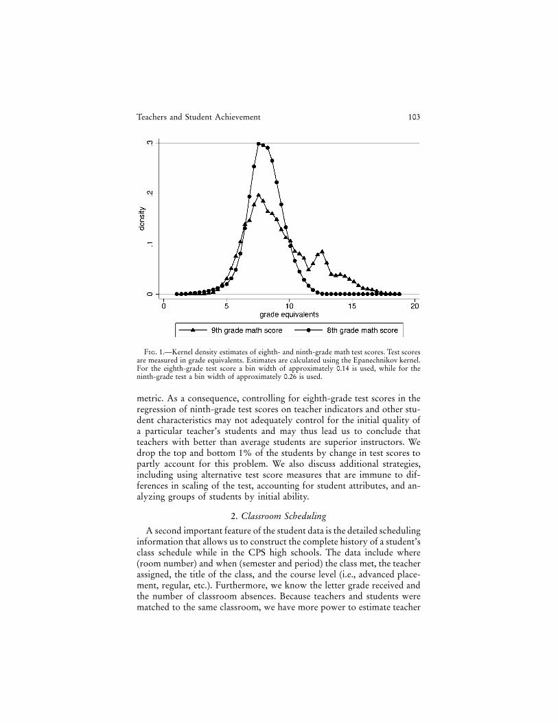
at least one ninth-grade student over our sample period, including instructorswho normally teach another subject or grade. The number of student-semestersfor each teacher over 3 years may be smaller than expected for several reasons(this is particularly evident in fig. 2 below). Most obviously, some teacher codesmay represent errors in the administrative data. Also, some codes may representtemporary vacancies. More importantly, Chicago Public Schools high schoolteachers teach students in multiple grades as well as in subjects other than math.In fact, most teachers of math classes in our analysis sample (89%) teach studentsof multiple grade levels. For the average teacher, 58% of her students are in theninth grade. In addition, roughly 40% of the teachers in the analysis sample alsoteach classes that are not math classes. Without excluding students for any reason,the teachers in our sample have an average of 189 unique students in all gradesand all subjects. Limiting the classes to math courses drops the average numberof students to 169. When we further limit the students to ninth graders, the averagenumber of students is 80.
Teachers and Student Achievement 107
third feature of the data: the detailed demographic and human capitalinformation supplied in the teacher administrative files. In particular, wecan use a teacher’s sex, race/ethnicity, experience, tenure, university at-tended, college major, advanced degree achievement, and teaching certi-fication to decompose total teacher effects into those related to commonobservable traits of teachers and those that are unobserved, such as drive,passion, and connection with students.
In order to match the teacher data to the student data we have toconstruct an alphanumeric code in the teacher data similar to the oneprovided in the student data. The teacher identifier in the student data isa combination of the teacher’s position number and letters from theteacher’s name, most often the first three letters of his or her last name.We make adjustments to the identifiers in cases for which the teachercodes in the student files do not match our constructed codes in the teacherdata due to discrepancies that arise for obvious reasons such as hyphenatedlast names, use of the first initial plus the first two letters of the last name,or transposed digits in the position number. Ultimately we are unable toresolve all of the mismatches between the student and teacher data butare able to match teacher characteristics to 75% of the teacher codes forwhich we estimate teacher quality (589 teachers). Table 3 provides de-scriptive statistics for the teachers we can match to the student admin-istrative records. The average teacher is 45 years old and has been in theCPS for 13 years. Minority math and computer science teachers are un-derrepresented relative to the student population, as 36% are AfricanAmerican and 10% Hispanic, but they compare more favorably to theoverall population of Chicago, which is 37% black or African Americanand 26% Hispanic or Latino (Census 2000 Fact Sheet for Chicago, U.S.Census Bureau). Eighty-two percent are certified to teach high school,37% are certified to be a substitute, and 10%–12% are certified to teachbilingual, elementary, or special education classes. The majority of mathteachers have a master’s degree, and many report a major in mathematics(48%) or education (18%).13
III. Basic Empirical Strategy
In the standard education production function, achievement, , of stu-Ydent i with teacher j in school k at time t is expressed as a function ofcumulative own, family, and peer inputs, X, from age 0 to the current
13 Nationally, 55% of high school teachers have a master’s degree, 66% havean academic degree (e.g., mathematics major), and 29% have a subject area ed-ucation degree (U.S. Department of Education 2000).

108 Aaronson et al.
Table 3Descriptive Statistics for the Teachers Matched to Math Teachersin the Student Data
Mean Standard Deviation
Demographics:Age 45.15 10.54Female .518 .500African American .360 .480White .469 .499Hispanic .100 .300Asian .063 .243Native American .007 .082
Human capital:BA major: education .182 .386BA major: all else .261 .440BA major: math .484 .500BA major: science .073 .260BA university, US News 1 .092 .289BA university, US News 2 .081 .274BA university, US News 3 .151 .358BA university, US News 4 .076 .266BA university, US News 5 .019 .135BA university, US News else .560 .497BA university missing .020 .141BA university local .587 .493Master’s degree .521 .500PhD .015 .123Certificate, bilingual education .119 .324Certificate, child .015 .123Certificate, elementary .100 .300Certificate, high school .823 .382Certificate, special education .107 .309Certificate, substitute .365 .482Potential experience 19.12 11.30Tenure at CPS 13.31 10.00Tenure in position 5.96 6.11
Number of observations 589
Note.—There are 783 teachers identified from the student estimation sample that haveat least 15 student-semesters for math classes over the 1997–99 sample period. The descriptivestatistics above apply to the subset of these teachers that can be matched to the teacheradministrative records from the Chicago Public Schools. US News rankings are from U.S.News & World Report (1995): level 1 p top tier universities (top 25 national universities �tier 1 national universities) � (top 25 national liberal arts colleges � tier 1 national liberalarts colleges); level 2 p second tier national universities � second tier national liberal artscolleges; level 3 p third tier national universities � third tier national liberal arts colleges;level 4 p fourth tier national universities � fourth tier national liberal arts colleges; andlevel 5 p top regional colleges and universities.
age, as well as cumulative teacher and school inputs, S, from grades kin-dergarten through the current grade:
T T
Y p b X � g S � � . (1)� �ijkt it ijkt ijkttp�5 tp0
The requirements to estimate (1) are substantial. Without a complete setof conditioning variables for X and S, omitted variables may bias estimatesof the coefficients on observable inputs unless strong and unlikely as-
Teachers and Student Achievement 109
sumptions about the covariance structure of observables and unobserv-ables are maintained. Thus, alternative identification strategies are typi-cally applied.
A simple approach is to take advantage of multiple test scores. In par-ticular, we estimate a general form of the value-added model by includingeighth-grade test scores as a covariate in explaining ninth-grade test scores.Lagged test scores account for the cumulative inputs of prior years whileallowing for a flexible autoregressive relationship in test scores. Con-trolling for past test scores is especially important with these data, asinformation on the family and pre-ninth-grade schooling is sparse.
We estimate an education production model of the general form
9 8Y p aY � bX � tT � v � r � � , (2)ikt it�1 i it i k ijkt
where refers to the ninth-grade test score of student i, who is enrolled9Yikt
in ninth grade at school k in year t; is the eighth-grade test score for8Yit�1
student i, who is enrolled in ninth grade in year t; and , , andv r �i k ijk
measure the unobserved impact of individuals, schools, and white noise,respectively.14 Each element of matrix Tit records the number of semestersspent in a math course with teacher j. To be clear, this is a cross-sectionalregression estimated using ordinary least squares with a slight deviationfrom the standard teacher fixed effect specification.15 Therefore, is thetj
jth element of the vector , representing the effect of one semester spentt
with math teacher j. Relative to equation (1), the impact of lagged school-ing and other characteristics is now captured by the lagged test scoremeasure.
While the value-added specification helps control for the fact that teach-ers may be assigned students with different initial ability on average, thisstrategy may still mismeasure teacher quality. For simplicity, assume thatall students have only one teacher for one semester so that the numberof student-semesters for teacher j equals the number of students, Nj. Inthis case, estimates of may be biased by .N Nj j1 1t r � � v � � �j k i ijktip1 ip1N Nj j
The school term is typically removed by including measures of schoolrk
quality, a general form of which is school fixed effects. School fixed effectsestimation is useful to control for time-invariant school characteristicsthat covary with individual teacher quality, without having to attributethe school’s contribution to specific measures. However, this strategyrequires the identification of teacher effects to be based on differences inthe number of semesters spent with a particular teacher and teachers thatswitch schools during our 3-year period. For short time periods, such as
14 All regressions include year indicators to control for any secular changes intest performance or reporting.
15 For repeaters, we use their first ninth-grade year so as to allow only a 1-yeargap between eighth- and ninth-grade test results.
110 Aaronson et al.
a single year, there may be little identifying variation to work with. Thus,this cleaner measure of the contribution of mathematics teachers comesat the cost of potential identifying variation. In addition, to the extentthat a principal is good because she is able to identify and hire high qualityteachers, some of the teacher quality may be attributed to the school. Forthese reasons, we show many results both with and without allowing forschool fixed effects.
Factors influencing test scores are often attributed to a student’s familybackground. In the context of gains, many researchers argue that time-invariant qualities are differenced out, leaving only time-varying influ-ences, such as parental divorce or a student’s introduction to drugs, in
. While undoubtedly working in gains lessens the omitted vari-Nj1 � viip1Nj
ables problem, we want to be careful not to claim that value-added frame-works completely eliminate it. In fact, it is quite reasonable to conjecturethat student gains vary with time-varying unobservables. But given ourstatistical model, bias is only introduced to the teacher quality rankingsif students are assigned to teachers based on these unobservable changes.16
Furthermore, we include a substantial list of observable student, family,and peer traits because they may be correlated with behavioral changesthat influence achievement and may account for group differences in gaintrajectories.
Finally, as the findings of Kane and Staiger (2002) make clear, the errorterm is particularly problematic when teacher fixed effect es-Nj1 � �ijktip1Nj
timates are based on small populations (small ). In this case, samplingNj
variation can overwhelm signal, causing a few good or bad draws tostrongly influence the estimated teacher fixed effect. Consequently, thestandard deviation of the distribution of estimated is most likely inflated.tj
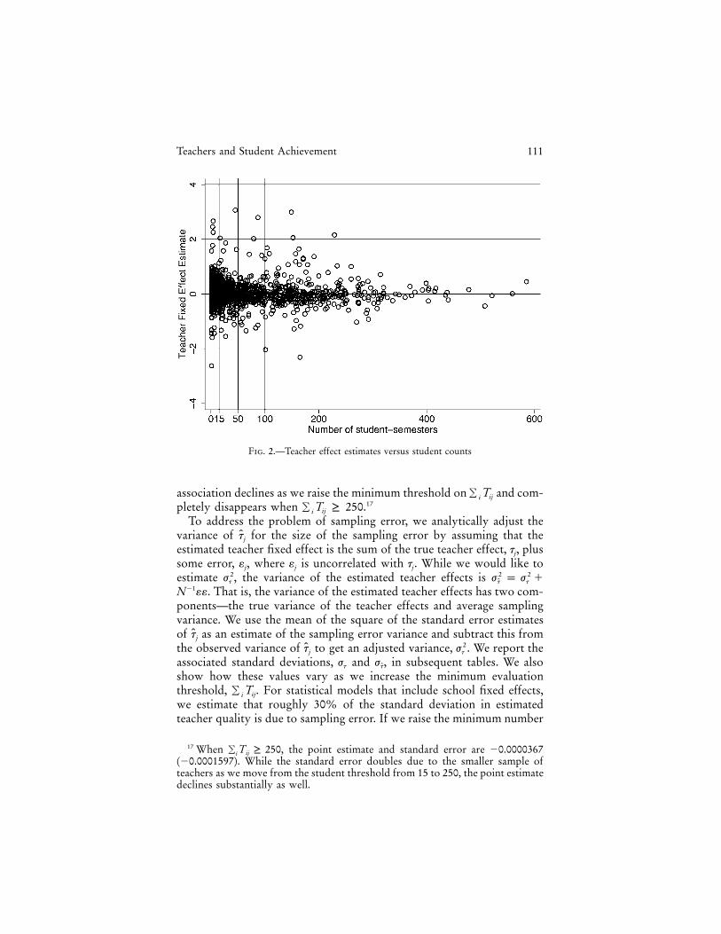
This problem is illustrated by figure 2, in which we plot our estimates(conditional on eighth-grade math score, year indicators, and student,tj
family, and peer attributes, as described below) against the number ofstudent-semesters on which the estimate is based. What is notable is thatthe lowest and highest performing teachers are those with the feweststudent-semesters. The expression represents the number of student-� Tiji
semesters taught by teacher j over the 3-year period examined (see n. 12for a discussion of the distribution of ). As more student-semesters� Tiji
are used to estimate the fixed effect, the importance of sampling variationdeclines and reliability improves. Regressing on summarizes thisˆFt F � Tj iji
association. Such an exercise has a coefficient estimate of �0.00045 witha standard error of 0.000076, suggesting that number of student-semestersis a critical correlate of the magnitude of estimated teacher quality. The
16 We do not discount the possibility of this type of sorting, especially fortransition schools, which are available to students close to expulsion. School fixedeffects pick this up, but we also estimate the results excluding these schools.
Teachers and Student Achievement 111
Fig. 2.—Teacher effect estimates versus student counts
association declines as we raise the minimum threshold on and com-� Tiji
pletely disappears when .17� T ≥ 250iji
To address the problem of sampling error, we analytically adjust thevariance of for the size of the sampling error by assuming that thetj
estimated teacher fixed effect is the sum of the true teacher effect, , plustj
some error, , where is uncorrelated with . While we would like to� � tj j j
estimate , the variance of the estimated teacher effects is2 2 2j j p j �ˆt t t
. That is, the variance of the estimated teacher effects has two com-�1N ��ponents—the true variance of the teacher effects and average samplingvariance. We use the mean of the square of the standard error estimatesof as an estimate of the sampling error variance and subtract this fromtj
the observed variance of to get an adjusted variance, . We report the2t jj t
associated standard deviations, and , in subsequent tables. We alsoj jˆt t
show how these values vary as we increase the minimum evaluationthreshold, . For statistical models that include school fixed effects,� Tiji
we estimate that roughly 30% of the standard deviation in estimatedteacher quality is due to sampling error. If we raise the minimum number
17 When , the point estimate and standard error are �0.0000367� T ≥ 250iji
(�0.0001597). While the standard error doubles due to the smaller sample ofteachers as we move from the student threshold from 15 to 250, the point estimatedeclines substantially as well.
112 Aaronson et al.
of student-semesters to identify an individual teacher to 200, only 14%of the standard deviation in teacher quality is due to sampling error.18
In the section to follow, we present our baseline estimates that ignorethe existence of most of these potential biases. We then report results thatattempt to deal with each potential bias. To the extent that real worldevaluation might not account for these problems, this exercise could beconsidered a cautionary tale of the extent to which teacher quality esti-mates can be interpreted incorrectly.
Finally, we examine whether teacher quality can be explained by de-mographic and human capital attributes of teachers. Because of concernsraised by Moulton (1986) about the efficiency of ordinary least squares(OLS) estimates in the presence of school-specific fixed effects and becausestudents are assigned multiple teachers per year, we do not include theteacher characteristics directly in equation (2). Rather, we employ a gen-eralized least squares (GLS) estimator outlined in Borjas (1987) and Borjasand Sueyoshi (1994). This estimator regresses on teacher characteristicstj
Z:
t p fZ � u . (3)j j j
The variance of the errors is calculated as the covariance matrix derivedfrom OLS estimates of (3) and the portion of equation (2)’s variance matrixrelated to the coefficient estimates, V.t
2Q p j I � V. (4)u J
The term in (4) is used to compute GLS estimates of the observableQ
teacher effects.
IV. Results
A. The Distribution of Teacher Quality
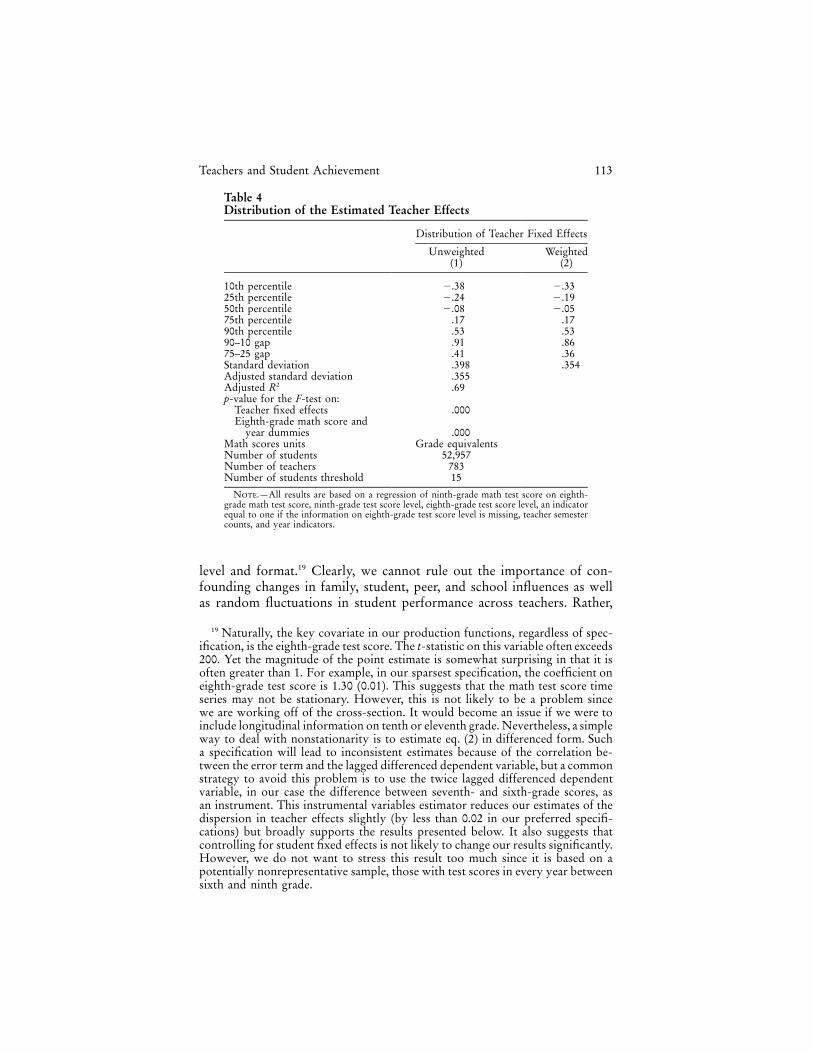
Our naive baseline estimates of teacher quality are presented in table4. In column 1 we present details on the distribution of , specificallytj
the standard deviation and the 10th, 25th, 50th, 75th, and 90th percentiles.We also list the p-value for an F-test of the joint significance of the teachereffects (i.e., for all j) and the p-value for an F-test of the othert p 0j
regressors. In this parsimonious specification, the list of regressors is lim-ited to eighth-grade math scores, year dummies, and indicators of the test
18 Note, however, that excluding teachers with small numbers of students islimiting because new teachers, particularly those for whom tenure decisions arebeing considered, may not be examined. This would be particularly troubling forelementary school teachers with fewer students per year.
Teachers and Student Achievement 113
Table 4Distribution of the Estimated Teacher Effects
Distribution of Teacher Fixed Effects
Unweighted(1)
Weighted(2)
10th percentile �.38 �.3325th percentile �.24 �.1950th percentile �.08 �.0575th percentile .17 .1790th percentile .53 .5390–10 gap .91 .8675–25 gap .41 .36Standard deviation .398 .354Adjusted standard deviation .355Adjusted R2 .69p-value for the F-test on:
Teacher fixed effects .000Eighth-grade math score and
year dummies .000Math scores units Grade equivalentsNumber of students 52,957Number of teachers 783Number of students threshold 15
Note.—All results are based on a regression of ninth-grade math test score on eighth-grade math test score, ninth-grade test score level, eighth-grade test score level, an indicatorequal to one if the information on eighth-grade test score level is missing, teacher semestercounts, and year indicators.
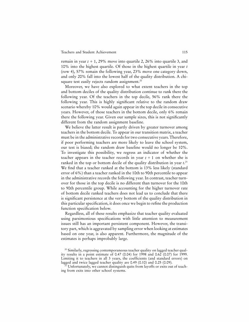
level and format.19 Clearly, we cannot rule out the importance of con-founding changes in family, student, peer, and school influences as wellas random fluctuations in student performance across teachers. Rather,
19 Naturally, the key covariate in our production functions, regardless of spec-ification, is the eighth-grade test score. The t-statistic on this variable often exceeds200. Yet the magnitude of the point estimate is somewhat surprising in that it isoften greater than 1. For example, in our sparsest specification, the coefficient oneighth-grade test score is 1.30 (0.01). This suggests that the math test score timeseries may not be stationary. However, this is not likely to be a problem sincewe are working off of the cross-section. It would become an issue if we were toinclude longitudinal information on tenth or eleventh grade. Nevertheless, a simpleway to deal with nonstationarity is to estimate eq. (2) in differenced form. Sucha specification will lead to inconsistent estimates because of the correlation be-tween the error term and the lagged differenced dependent variable, but a commonstrategy to avoid this problem is to use the twice lagged differenced dependentvariable, in our case the difference between seventh- and sixth-grade scores, asan instrument. This instrumental variables estimator reduces our estimates of thedispersion in teacher effects slightly (by less than 0.02 in our preferred specifi-cations) but broadly supports the results presented below. It also suggests thatcontrolling for student fixed effects is not likely to change our results significantly.However, we do not want to stress this result too much since it is based on apotentially nonrepresentative sample, those with test scores in every year betweensixth and ninth grade.
114 Aaronson et al.
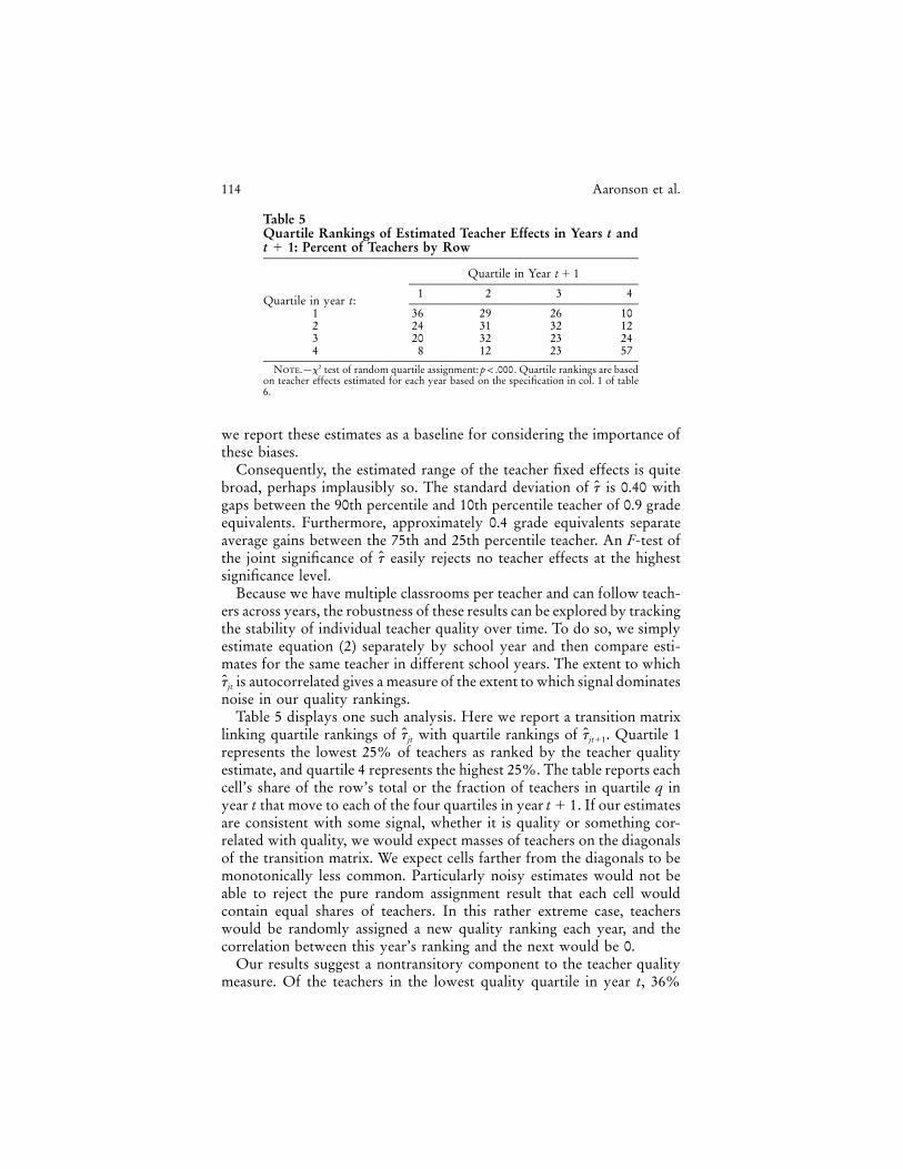
Table 5Quartile Rankings of Estimated Teacher Effects in Years t andt � 1: Percent of Teachers by Row
Quartile in Year t � 1
Quartile in year t:1 2 3 4
1 36 29 26 102 24 31 32 123 20 32 23 244 8 12 23 57
Note.— test of random quartile assignment: . Quartile rankings are based2x p ! .000on teacher effects estimated for each year based on the specification in col. 1 of table6.
we report these estimates as a baseline for considering the importance ofthese biases.
Consequently, the estimated range of the teacher fixed effects is quitebroad, perhaps implausibly so. The standard deviation of is 0.40 witht
gaps between the 90th percentile and 10th percentile teacher of 0.9 gradeequivalents. Furthermore, approximately 0.4 grade equivalents separateaverage gains between the 75th and 25th percentile teacher. An F-test ofthe joint significance of easily rejects no teacher effects at the highestt
significance level.Because we have multiple classrooms per teacher and can follow teach-
ers across years, the robustness of these results can be explored by trackingthe stability of individual teacher quality over time. To do so, we simplyestimate equation (2) separately by school year and then compare esti-mates for the same teacher in different school years. The extent to which
is autocorrelated gives a measure of the extent to which signal dominatestjt
noise in our quality rankings.Table 5 displays one such analysis. Here we report a transition matrix
linking quartile rankings of with quartile rankings of . Quartile 1ˆ ˆt tjt jt�1
represents the lowest 25% of teachers as ranked by the teacher qualityestimate, and quartile 4 represents the highest 25%. The table reports eachcell’s share of the row’s total or the fraction of teachers in quartile q inyear t that move to each of the four quartiles in year . If our estimatest � 1are consistent with some signal, whether it is quality or something cor-related with quality, we would expect masses of teachers on the diagonalsof the transition matrix. We expect cells farther from the diagonals to bemonotonically less common. Particularly noisy estimates would not beable to reject the pure random assignment result that each cell wouldcontain equal shares of teachers. In this rather extreme case, teacherswould be randomly assigned a new quality ranking each year, and thecorrelation between this year’s ranking and the next would be 0.
Our results suggest a nontransitory component to the teacher qualitymeasure. Of the teachers in the lowest quality quartile in year t, 36%
Teachers and Student Achievement 115
remain in year , 29% move into quartile 2, 26% into quartile 3, andt � 110% into the highest quartile. Of those in the highest quartile in year t(row 4), 57% remain the following year, 23% move one category down,and only 20% fall into the lowest half of the quality distribution. A chi-square test easily rejects random assignment.20
Moreover, we have also explored to what extent teachers in the topand bottom deciles of the quality distribution continue to rank there thefollowing year. Of the teachers in the top decile, 56% rank there thefollowing year. This is highly significant relative to the random drawscenario whereby 10% would again appear in the top decile in consecutiveyears. However, of those teachers in the bottom decile, only 6% remainthere the following year. Given our sample sizes, this is not significantlydifferent from the random assignment baseline.
We believe the latter result is partly driven by greater turnover amongteachers in the bottom decile. To appear in our transition matrix, a teachermust be in the administrative records for two consecutive years. Therefore,if poor performing teachers are more likely to leave the school system,our test is biased; the random draw baseline would no longer be 10%.To investigate this possibility, we regress an indicator of whether theteacher appears in the teacher records in year on whether she ist � 1ranked in the top or bottom decile of the quality distribution in year t.21
We find that a teacher ranked at the bottom is 13% less likely (standarderror of 6%) than a teacher ranked in the 10th to 90th percentile to appearin the administrative records the following year. In contrast, teacher turn-over for those in the top decile is no different than turnover for the 10thto 90th percentile group. While accounting for the higher turnover rateof bottom decile ranked teachers does not lead us to conclude that thereis significant persistence at the very bottom of the quality distribution inthis particular specification, it does once we begin to refine the productionfunction specification below.
Regardless, all of these results emphasize that teacher quality evaluatedusing parsimonious specifications with little attention to measurementissues still has an important persistent component. However, the transi-tory part, which is aggravated by sampling error when looking at estimatesbased on one year, is also apparent. Furthermore, the magnitude of theestimates is perhaps improbably large.
20 Similarly, regressing contemporaneous teacher quality on lagged teacher qual-ity results in a point estimate of 0.47 (0.04) for 1998 and 0.62 (0.07) for 1999.Limiting it to teachers in all 3 years, the coefficients (and standard errors) onlagged and twice lagged teacher quality are 0.49 (0.10) and 0.25 (0.09).
21 Unfortunately, we cannot distinguish quits from layoffs or exits out of teach-ing from exits into other school systems.
116 Aaronson et al.
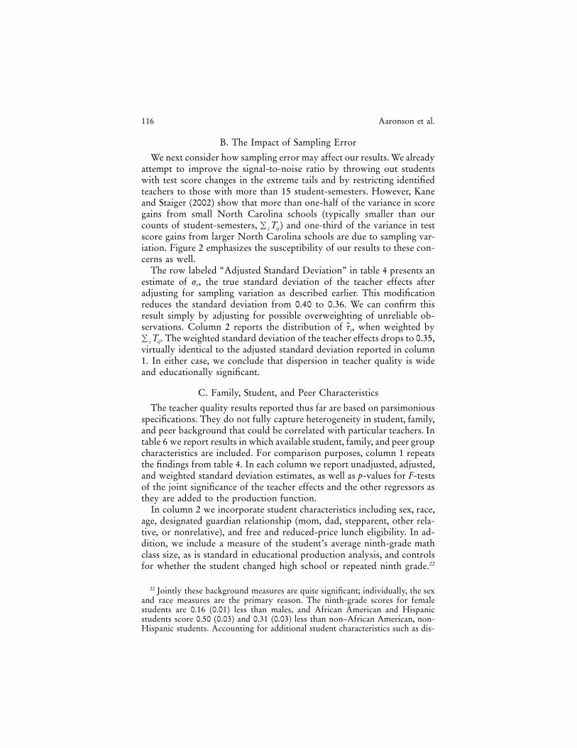
B. The Impact of Sampling Error
We next consider how sampling error may affect our results. We alreadyattempt to improve the signal-to-noise ratio by throwing out studentswith test score changes in the extreme tails and by restricting identifiedteachers to those with more than 15 student-semesters. However, Kaneand Staiger (2002) show that more than one-half of the variance in scoregains from small North Carolina schools (typically smaller than ourcounts of student-semesters, ) and one-third of the variance in test� Tiji
score gains from larger North Carolina schools are due to sampling var-iation. Figure 2 emphasizes the susceptibility of our results to these con-cerns as well.
The row labeled “Adjusted Standard Deviation” in table 4 presents anestimate of , the true standard deviation of the teacher effects afterjt
adjusting for sampling variation as described earlier. This modificationreduces the standard deviation from 0.40 to 0.36. We can confirm thisresult simply by adjusting for possible overweighting of unreliable ob-servations. Column 2 reports the distribution of , when weighted bytj
. The weighted standard deviation of the teacher effects drops to 0.35,� Tiji
virtually identical to the adjusted standard deviation reported in column1. In either case, we conclude that dispersion in teacher quality is wideand educationally significant.
C. Family, Student, and Peer Characteristics
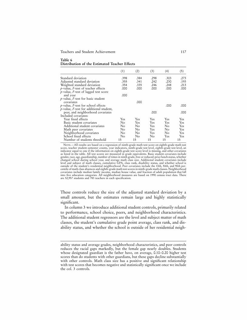
The teacher quality results reported thus far are based on parsimoniousspecifications. They do not fully capture heterogeneity in student, family,and peer background that could be correlated with particular teachers. Intable 6 we report results in which available student, family, and peer groupcharacteristics are included. For comparison purposes, column 1 repeatsthe findings from table 4. In each column we report unadjusted, adjusted,and weighted standard deviation estimates, as well as p-values for F-testsof the joint significance of the teacher effects and the other regressors asthey are added to the production function.
In column 2 we incorporate student characteristics including sex, race,age, designated guardian relationship (mom, dad, stepparent, other rela-tive, or nonrelative), and free and reduced-price lunch eligibility. In ad-dition, we include a measure of the student’s average ninth-grade mathclass size, as is standard in educational production analysis, and controlsfor whether the student changed high school or repeated ninth grade.22
22 Jointly these background measures are quite significant; individually, the sexand race measures are the primary reason. The ninth-grade scores for femalestudents are 0.16 (0.01) less than males, and African American and Hispanicstudents score 0.50 (0.03) and 0.31 (0.03) less than non–African American, non-Hispanic students. Accounting for additional student characteristics such as dis-
Teachers and Student Achievement 117
Table 6Distribution of the Estimated Teacher Effects
(1) (2) (3) (4) (5)
Standard deviation .398 .384 .298 .303 .273Adjusted standard deviation .355 .341 .242 .230 .193Weighted standard deviation .354 .335 .246 .248 .213p-value, F-test of teacher effects .000 .000 .000 .000 .000p-value, F-test of lagged test score
and year .000p-value, F-test for basic student
covariates .000p-value, F-test for school effects .000 .000p-value, F-test for additional student,
peer, and neighborhood covariates .000 .000Included covariates:
Year fixed effects Yes Yes Yes Yes YesBasic student covariates No Yes Yes Yes YesAdditional student covariates No No Yes No YesMath peer covariates No No Yes No YesNeighborhood covariates No No Yes No YesSchool fixed effects No No No Yes YesNumber of students threshold 15 15 15 15 15
Note.—All results are based on a regression of ninth-grade math test score on eighth-grade math testscore, teacher student-semester counts, year indicators, ninth-grade test level, eighth-grade test level, anindicator equal to one if the information on eighth-grade test score level is missing, and other covariatesas listed in the table. All test scores are measured in grade equivalents. Basic student covariates includegender, race, age, guardianship, number of times in ninth grade, free or reduced-price lunch status, whetherchanged school during school year, and average math class size. Additional student covariates includelevel and subject of math classes, cumulative GPA, class rank, disability status, and whether school isoutside of the student’s residential neighborhood. Peer covariates include the 10th, 50th, and 90th per-centile of math class absences and eighth-grade math test scores in ninth-grade math classes. Neighborhoodcovariates include median family income, median house value, and fraction of adult population that fallinto five education categories. All neighborhood measures are based on 1990 census tract data. Thereare 52,957 students and 783 teachers in each specification.
These controls reduce the size of the adjusted standard deviation by asmall amount, but the estimates remain large and highly statisticallysignificant.
In column 3 we introduce additional student controls, primarily relatedto performance, school choice, peers, and neighborhood characteristics.The additional student regressors are the level and subject matter of mathclasses, the student’s cumulative grade point average, class rank, and dis-ability status, and whether the school is outside of her residential neigh-
ability status and average grades, neighborhood characteristics, and peer controlsreduces the racial gaps markedly, but the female gap nearly doubles. Studentswhose designated guardian is the father have, on average, 0.10–0.20 higher testscores than do students with other guardians, but these gaps decline substantiallywith other controls. Math class size has a positive and significant relationshipwith test scores that becomes negative and statistically significant once we includethe col. 3 controls.
118 Aaronson et al.
borhood.23 The neighborhood measures are based on Census data for astudent’s residential census tract and include median family income, me-dian house value, and the fraction of adults that fall into five educationcategories. These controls are meant to proxy for unobserved parentalinfluences. Again, like many of the student controls, the value-addedframework should, for example, account for permanent income gaps butnot for differences in student growth rates by parental income or edu-cation. Finally, the math class peer characteristics are the 10th, 50th, and90th percentiles of absences, as a measure of disruption in the classroom,and the same percentiles of eighth-grade math test scores, as a measureof peer ability. Because teacher ability may influence classroom attendancepatterns, peer absences could confound our estimates of interest, leadingto downward biased teacher quality estimates.24
Adding student, peer, and neighborhood covariates reduces the adjustedstandard deviation to 0.24, roughly two-thirds the size of the naive es-timates reported in column 1.25 Much of the attenuation comes fromadding either own or peer performance measures. Nevertheless, regardlessof the controls introduced, the dispersion in teacher quality remains largeand statistically significant.
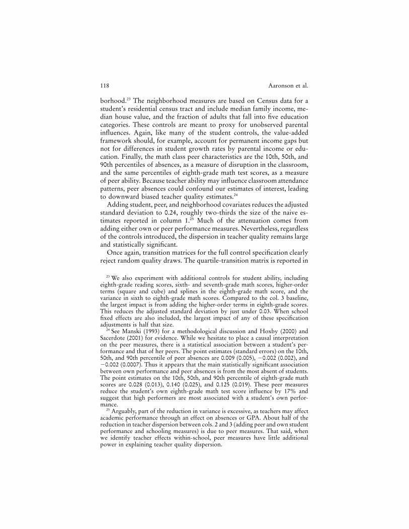
Once again, transition matrices for the full control specification clearlyreject random quality draws. The quartile-transition matrix is reported in
23 We also experiment with additional controls for student ability, includingeighth-grade reading scores, sixth- and seventh-grade math scores, higher-orderterms (square and cube) and splines in the eighth-grade math score, and thevariance in sixth to eighth-grade math scores. Compared to the col. 3 baseline,the largest impact is from adding the higher-order terms in eighth-grade scores.This reduces the adjusted standard deviation by just under 0.03. When schoolfixed effects are also included, the largest impact of any of these specificationadjustments is half that size.
24 See Manski (1993) for a methodological discussion and Hoxby (2000) andSacerdote (2001) for evidence. While we hesitate to place a causal interpretationon the peer measures, there is a statistical association between a student’s per-formance and that of her peers. The point estimates (standard errors) on the 10th,50th, and 90th percentile of peer absences are 0.009 (0.005), �0.002 (0.002), and�0.002 (0.0007). Thus it appears that the main statistically significant associationbetween own performance and peer absences is from the most absent of students.The point estimates on the 10th, 50th, and 90th percentile of eighth-grade mathscores are 0.028 (0.013), 0.140 (0.025), and 0.125 (0.019). These peer measuresreduce the student’s own eighth-grade math test score influence by 17% andsuggest that high performers are most associated with a student’s own perfor-mance.
25 Arguably, part of the reduction in variance is excessive, as teachers may affectacademic performance through an effect on absences or GPA. About half of thereduction in teacher dispersion between cols. 2 and 3 (adding peer and own studentperformance and schooling measures) is due to peer measures. That said, whenwe identify teacher effects within-school, peer measures have little additionalpower in explaining teacher quality dispersion.
Teachers and Student Achievement 119
Table 7Quartile Rankings of Estimated Teacher Effects in Years t andt � 1: Percent of Teachers by Row
Quartile in Year t � 1
Quartile in year t:1 2 3 4
1 33 32 16 192 32 25 31 133 17 25 33 264 15 21 23 41
Note.—x2 test of random quartile assignment: . Quartile rankings are basedp ! .001on teacher effects estimated for each year based on the specification including laggedmath test score, year indicators, and all student, peer, and neighborhood covariates(col. 3 of table 6).
table 7. Forty-one percent of teachers ranking in the top 25% in one yearrank in the top 25% in the following year. Another 23% slip down onecategory, 21% two categories, and 15% to the bottom category.26
D. Within-School Estimates
Within-school variation in teacher quality is often preferred to the be-tween-school variety as it potentially eliminates time-invariant school-level factors. In our case, since we are looking over a relatively shortwindow (3 years), this might include the principal, curriculum, schoolsize or composition, quality of other teachers in the school, and latentfamily or neighborhood-level characteristics that can influence schoolchoice. Because our results are based on achievement gains, we are gen-erally concerned only with changes in these factors. Therefore, restrictingthe source of teacher variation to within-school differences will result ina more consistent, but less precisely estimated, measure of the contributionof teachers.
Our primary method of controlling for school-level influences is schoolfixed effects. As mentioned above, identification depends on differencesin the intensity of students’ exposure to different teachers within schools,as well as teachers switching schools during the sample period.27 We reportthese results in columns 4 and 5 of table 6. Relative to the analogouscolumns without school fixed effects, the dispersion in teacher qualityand precision of the estimates decline. For example, with the full set ofstudent controls, the adjusted standard deviation drops from 0.24 (col. 3)
26 Twenty-six percent and 19% of those in the top and bottom deciles remainthe next year. Nineteen percent and 14% rated in the top and bottom deciles in1997 are still there in 1999. Again, turnover is 15% higher among the lowestperforming teachers. Adjusting for this extra turnover , the p-value on the bottomdecile transition F-test drops from 0.14 to 0.06.
27 Of the teachers with at least 15 student-semester observations, 69% appearin one school over the 3 years and 18% appear in two schools. Additionally,13%–17% of teachers in each year show up in multiple schools.
120 Aaronson et al.
Table 8Correlation between Teacher Quality Estimates across Specifications
Specification Relative to Baseline
Minimum Number ofStudent-Semesters Required
to Identify a Teacher
15(1)
100(2)
200(3)
(0) Baseline 1.00 1.00 1.00(1) Drop neighborhood covariates 1.00 1.00 1.00(2) Drop peer covariates .97 .98 .99(3) Drop additional student covariates .92 .93 .94(4) Drop basic student covariates .99 1.00 1.00(5) Drop basic and additional student, peer,
and neighborhood characteristics .88 .85 .87(6) Drop school fixed effects .86 .68 .65(7) Drop school fixed effects and basic and
additional student, peer, and neighborhoodcharacteristics .62 .44 .45
Number of teachers 783 317 122
Note.—The col. 1 baseline corresponds to the results presented in col. 5 of table 6. Columns 2 and3 correspond to the results presented in table 9, cols. 2 and 3, respectively. All specifications include theeighth-grade math test score, teacher student-semester counts, year indicators, the ninth-grade test level,the eighth-grade test level, an indicator equal to one if the information on eighth-grade test schore levelis missing, and a constant. The baseline specification additionally includes basic and additional studentcharacteristics, neighborhood and peer characteristics, and school fixed effects. All other specificationsinclude a subset of these controls as noted in the table. See table 6 for the specific variables in each group.
to 0.19 (col. 5), roughly one-half the impact from the unadjusted value-added model reported in column 1. Again, an F-test rejects that the within-school teacher quality estimates jointly equal zero at the 1% level. Wehave also estimated column 4 and 5 models when allowing for school-specific time effects, to account for changes in principals, curricula, andother policies, and found nearly identical results. The adjusted standarddeviations are 0.23 and 0.18, respectively, just 0.01 lower than estimatesreported in the table.
Notably, however, once we look within schools, sampling variationaccounts for roughly one-third of the unadjusted standard deviation inteacher quality. Furthermore, sampling variation becomes even moreproblematic when we estimate year-to-year transitions in quality, as intables 5 and 7, with specifications that control for school fixed effects.
E. Robustness of Teacher Quality Estimates across Specifications
One critique of using test score based measurements to assess teachereffectiveness has been that quality rankings can be sensitive to how theyare calculated. We suspect that using measures of teacher effectiveness thatdiffer substantially under alternative, but reasonable, specifications ofequation (2) will weaken program incentives to increase teacher effort inorder to improve student achievement. To gauge how sensitive our resultsare to the inclusion of various controls, table 8 reports the robustness of
Teachers and Student Achievement 121
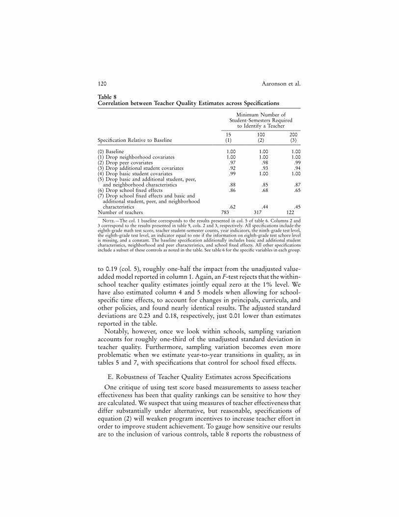
the teacher rankings to various permutations of our baseline results (col.5 of table 6). In particular, we present the correlations of our teacherquality estimate based on our preferred statistical model—which controlsfor school fixed effects as well as student, peer, and neighborhood char-acteristics—with estimates from alternative specifications.
Because the estimation error is likely to be highly correlated acrossspecifications, we calculate the correlation between estimates using em-pirical Bayes estimates of teacher effects (e.g., Kane and Staiger 2002). Werescale the OLS estimates using estimates of the true variation in teachereffects and the estimation error as follows:
2jtˆt* p t 7 , (5)j j 2 2ˆj � jt �
where is our OLS estimate of the value added by teacher j, is our2t jj t
estimate of the true variation in teacher effects (calculated as describedabove), and is the noise associated with the estimate of teacher j’s effect,2j�
namely, the estimation error for . To further minimize concern abouttj
sampling variability, we also look at correlations across specifications es-timated from samples of teachers that have at least 100 or 200 studentsduring our period.
In rows 1–4, we begin by excluding, in order, residential neighborhood,peer, student background, and student performance covariates. Individ-ually, each of these groups of variables has little impact on the rankings.Teacher rankings are always correlated at least 0.92 with the baseline.Even when we drop all of the right-hand-side covariates, except schoolfixed effects, row 5 shows that the teacher ranking correlations are stillquite high, ranging from 0.85 to 0.88.
Only when school fixed effects are excluded is there a notable drop inthe correlation with the baseline. In row 6, we exclude school fixed effectsbut leave the other covariates in place. The teacher quality correlationfalls to between 0.65 and 0.86. Excluding the other right-hand-side co-variates causes the correlation to fall to between 0.44 and 0.62. That is,without controlling for school fixed effects, rankings become quite sen-sitive to the statistical model. But as long as we consider within-schoolteacher quality rankings using a value-added specification, the estimatesare highly correlated across specifications, regardless of the other controlsincluded.
Importantly, our results imply that teacher rankings based on test scoregains are quite robust to the modeling choices that are required for anindividual principal to rank her own teachers. But a principal may havemore difficulty evaluating teachers outside her home school. More gen-erally, value-added estimates that do not account for differences across

122 Aaronson et al.
schools may vary widely based on specification choices which in turnmay weaken teacher performance incentives.
F. Additional Robustness Checks
Thus far, we have found that teacher quality varies substantially acrossteachers, even within the same school, and is fairly robust across reason-able value-added regression specifications. This section provides addi-tional evidence on the robustness of our results to strategic test scorereporting, sampling variability, test normalization, and the inclusion ofother teachers in the math score production function.
1. Cream Skimming
One concern is that teachers or schools discourage some students fromtaking exams because they are expected to perform poorly. If such creamskimming is taking place, we might expect to see a positive correlationbetween our teacher quality measures tj and the share of teacher j’s stu-dents that are missing ninth-grade test scores. In fact, we find that thiscorrelation is small (�0.02), opposite in sign to this cream-skimmingprediction, and not statistically different from zero.
Another way to game exam results is for teachers or schools to teststudents whose scores are not required to be reported and then reportscores only for those students who do well. To examine this possibility,we calculate the correlation between teacher quality and the share ofstudents excluded from exam reporting.28 In this case, evidence is con-sistent with gaming of scores; the correlation is positive (0.07) and sta-tistically different from zero at the 6% level. To gauge the importance ofthis finding for our results, we reran our statistical models, dropping allstudents for whom test scores may be excluded from school and districtreporting. This exclusion affected 6,361 students (12% of the full sample)but had no substantive impact on our results.
2. Sampling Variability: Restrictions onStudent-Semester Observations
A simple strategy for minimizing sampling variability is to restrict eval-uation to teachers with a large number of student-semesters. In table 9,we explore limiting assessment of teacher dispersion to teachers with atleast 50, 100, or 200 student-semesters. We emphasize that a samplingrestriction, while useful for its simplicity, can be costly in terms of in-ference. Obviously, the number of teachers for whom we can estimatequality is reduced. There may also be an issue about how representative
28 The student test file includes an indicator for whether the student’s test scoremay be excluded from reported school or citywide test score statistics because,e.g., the student is a special or bilingual education student.
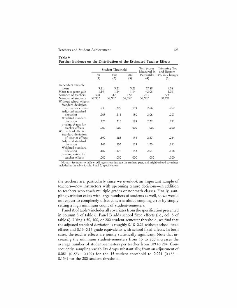
Teachers and Student Achievement 123
Table 9Further Evidence on the Distribution of the Estimated Teacher Effects
Student Threshold Test ScoresMeasured inPercentiles
(4)
Trimming Topand Bottom
3% in Changes(5)
50(1)
100(2)
200(3)
Dependent variablemean 9.21 9.21 9.21 37.88 9.08
Mean test score gain 1.14 1.14 1.14 �2.08 1.06Number of teachers 508 317 122 783 773Number of students 52,957 52,957 52,957 52,957 50,392Without school effects:
Standard deviationof teacher effects .233 .227 .193 2.66 .262
Adjusted standarddeviation .205 .211 .180 2.06 .203
Weighted standarddeviation .223 .216 .188 2.22 .211
p-value, F-test forteacher effects .000 .000 .000 .000 .000
With school effects:Standard deviation
of teacher effects .192 .183 .154 2.57 .244Adjusted standard
deviation .143 .155 .133 1.75 .161Weighted standard
deviation .182 .176 .152 2.04 .188p-value, F-test for
teacher effects .000 .000 .000 .000 .000
Note.—See notes to table 6. All regressions include the student, peer, and neighborhood covariatesincluded in the table 6, cols. 3 and 5, specifications.
the teachers are, particularly since we overlook an important sample ofteachers—new instructors with upcoming tenure decisions—in additionto teachers who teach multiple grades or nonmath classes. Finally, sam-pling variation exists with large numbers of students as well, so we wouldnot expect to completely offset concerns about sampling error by simplysetting a high minimum count of student-semesters.
Panel A of table 9 includes all covariates from the specification presentedin column 3 of table 6. Panel B adds school fixed effects (i.e., col. 5 oftable 6). Using a 50, 100, or 200 student-semester threshold, we find thatthe adjusted standard deviation is roughly 0.18–0.21 without school fixedeffects and 0.13–0.15 grade equivalents with school fixed effects. In bothcases, the teacher effects are jointly statistically significant. Note that in-creasing the minimum student-semesters from 15 to 200 increases theaverage number of student-semesters per teacher from 109 to 284. Con-sequently, sampling variability drops substantially, from an adjustment of0.081 ( ) for the 15-student threshold to 0.021 (0.273 � 0.192 0.155 �
) for the 200-student threshold.0.134
124 Aaronson et al.
3. More on Test Score Normalization and the UndueInfluence of Outliers
The remaining columns of table 9 include attempts to minimize theinfluence of outlier observations. Column 4 reports findings using nationalpercentile rankings that are impervious to the normalization probleminherent in grade-equivalent scores.29 We find that the adjusted standarddeviation of is 1.75 percentile points, a result that is statistically andtj
educationally significant and broadly consistent with the grade-equivalentresults.
In the next column, we simply trim the top and bottom 3% of thedistribution of eighth- to ninth-grade math test gains from the studentsample. We would clearly expect that this sample restriction would reducethe variance, as it eliminates roughly 2,600 students in the tails of thescore distribution. Still, the adjusted teacher standard deviation remainslarge in magnitude and statistically significant at 0.16 grade equivalents.30
4. Including Other Teachers in the Production Function
We explore one final specification that takes advantage of the detailedclassroom scheduling in our data by including a full set of English teachersemester counts, akin to the math teacher semester count, Ti, in equation(2). Assuming that the classroom-sorting mechanism is similar across sub-ject areas (e.g., parents who demand the best math teacher will also demandthe best English teacher or schools will sort students into classrooms andassign classes to teachers based on the students’ expected test score gains),the English teachers will pick up some sorting that may confound esti-mates of . Moreover, the English teachers may help us gauge the im-t
portance of teacher externalities, that is, the proverbial superstar teacherwho inspires students to do well not just in her class but in all classes.In the presence of student sorting by teacher quality, these spillover effectswill exacerbate the bias in the math teacher quality estimates. Althoughwe cannot separately identify classroom sorting from teacher spillovers,
29 These rankings have the advantage of potentially greater consistency acrosstests so long as the reference population of test takers is constant. The publisherof the tests, Riverside Publishing, advertises the TAP as being “fully articulated”with the ITBS and useful for tracking student progress. Less than 2% of thesample is censored, of which over 98% are at the lowest possible percentile scoreof 1. Estimates using a Tobit to account for this censoring problem result invirtually identical coefficient estimates and estimates of the standard deviation ofthe .tj
30 We have also tried using the robust estimator developed by Huber to accountfor outliers. The technique weights observations based on an initial regressionand is useful for its high degree of efficiency in the face of heavy-tailed data.These results generate an even wider distribution of estimated teacher quality.
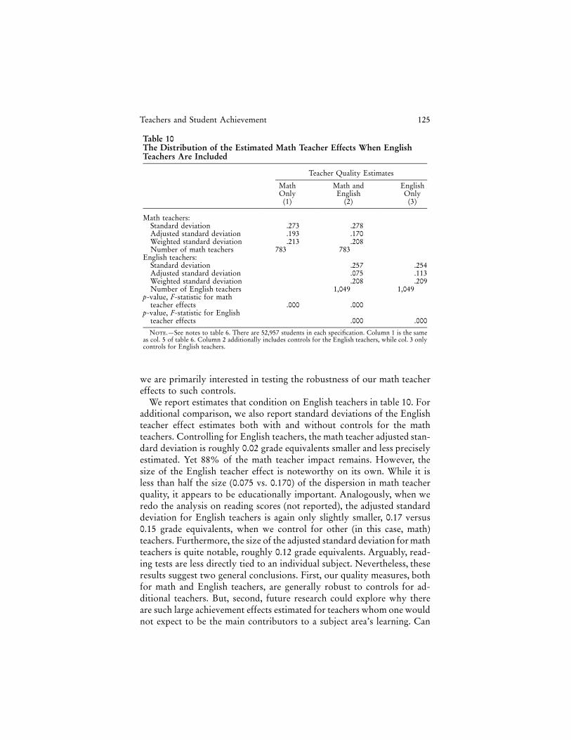
Teachers and Student Achievement 125
Table 10The Distribution of the Estimated Math Teacher Effects When EnglishTeachers Are Included
Teacher Quality Estimates
MathOnly
(1)
Math andEnglish
(2)
EnglishOnly
(3)
Math teachers:Standard deviation .273 .278Adjusted standard deviation .193 .170Weighted standard deviation .213 .208Number of math teachers 783 783
English teachers:Standard deviation .257 .254Adjusted standard deviation .075 .113Weighted standard deviation .208 .209Number of English teachers 1,049 1,049
p-value, F-statistic for mathteacher effects .000 .000
p-value, F-statistic for Englishteacher effects .000 .000
Note.—See notes to table 6. There are 52,957 students in each specification. Column 1 is the sameas col. 5 of table 6. Column 2 additionally includes controls for the English teachers, while col. 3 onlycontrols for English teachers.
we are primarily interested in testing the robustness of our math teachereffects to such controls.
We report estimates that condition on English teachers in table 10. Foradditional comparison, we also report standard deviations of the Englishteacher effect estimates both with and without controls for the mathteachers. Controlling for English teachers, the math teacher adjusted stan-dard deviation is roughly 0.02 grade equivalents smaller and less preciselyestimated. Yet 88% of the math teacher impact remains. However, thesize of the English teacher effect is noteworthy on its own. While it isless than half the size (0.075 vs. 0.170) of the dispersion in math teacherquality, it appears to be educationally important. Analogously, when weredo the analysis on reading scores (not reported), the adjusted standarddeviation for English teachers is again only slightly smaller, 0.17 versus0.15 grade equivalents, when we control for other (in this case, math)teachers. Furthermore, the size of the adjusted standard deviation for mathteachers is quite notable, roughly 0.12 grade equivalents. Arguably, read-ing tests are less directly tied to an individual subject. Nevertheless, theseresults suggest two general conclusions. First, our quality measures, bothfor math and English teachers, are generally robust to controls for ad-ditional teachers. But, second, future research could explore why thereare such large achievement effects estimated for teachers whom one wouldnot expect to be the main contributors to a subject area’s learning. Can
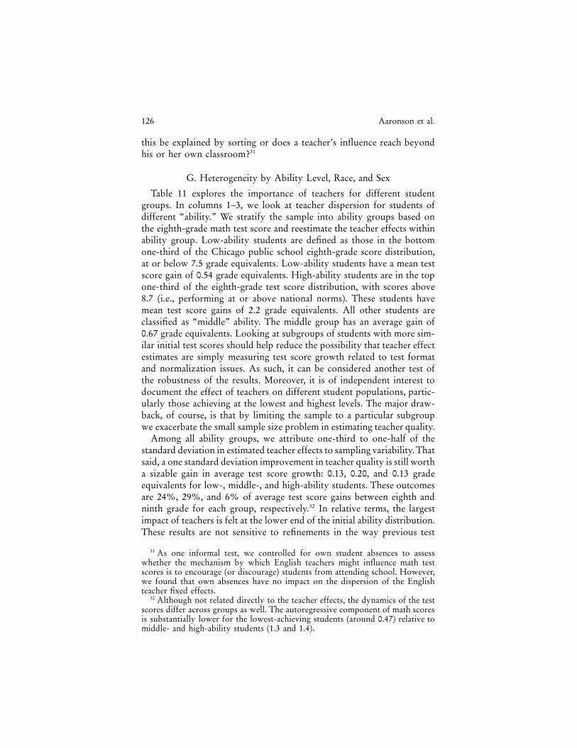
126 Aaronson et al.
this be explained by sorting or does a teacher’s influence reach beyondhis or her own classroom?31
G. Heterogeneity by Ability Level, Race, and Sex
Table 11 explores the importance of teachers for different studentgroups. In columns 1–3, we look at teacher dispersion for students ofdifferent “ability.” We stratify the sample into ability groups based onthe eighth-grade math test score and reestimate the teacher effects withinability group. Low-ability students are defined as those in the bottomone-third of the Chicago public school eighth-grade score distribution,at or below 7.5 grade equivalents. Low-ability students have a mean testscore gain of 0.54 grade equivalents. High-ability students are in the topone-third of the eighth-grade test score distribution, with scores above8.7 (i.e., performing at or above national norms). These students havemean test score gains of 2.2 grade equivalents. All other students areclassified as “middle” ability. The middle group has an average gain of0.67 grade equivalents. Looking at subgroups of students with more sim-ilar initial test scores should help reduce the possibility that teacher effectestimates are simply measuring test score growth related to test formatand normalization issues. As such, it can be considered another test ofthe robustness of the results. Moreover, it is of independent interest todocument the effect of teachers on different student populations, partic-ularly those achieving at the lowest and highest levels. The major draw-back, of course, is that by limiting the sample to a particular subgroupwe exacerbate the small sample size problem in estimating teacher quality.
Among all ability groups, we attribute one-third to one-half of thestandard deviation in estimated teacher effects to sampling variability. Thatsaid, a one standard deviation improvement in teacher quality is still wortha sizable gain in average test score growth: 0.13, 0.20, and 0.13 gradeequivalents for low-, middle-, and high-ability students. These outcomesare 24%, 29%, and 6% of average test score gains between eighth andninth grade for each group, respectively.32 In relative terms, the largestimpact of teachers is felt at the lower end of the initial ability distribution.These results are not sensitive to refinements in the way previous test
31 As one informal test, we controlled for own student absences to assesswhether the mechanism by which English teachers might influence math testscores is to encourage (or discourage) students from attending school. However,we found that own absences have no impact on the dispersion of the Englishteacher fixed effects.
32 Although not related directly to the teacher effects, the dynamics of the testscores differ across groups as well. The autoregressive component of math scoresis substantially lower for the lowest-achieving students (around 0.47) relative tomiddle- and high-ability students (1.3 and 1.4).
Table 11Distribution of the Estimated Teacher Effects for Selected Student Subgroups
Ability Level Race/Ethnicity Sex
Low(1)
Middle(2)
High(3)
Non–African American,Non-Hispanic
(4)
AfricanAmerican
(5)Hispanic
(6)Male(7)
Female(8)
Mean gain .54 .67 2.22 2.19 .86 1.19 1.22 1.06Standard deviation .236 .304 .274 .259 .293 .248 .303 .264Adjusted standard deviation .129 .196 .132 .105 .201 .132 .201 .160p-value, F-statistic for
teacher effects .000 .000 .000 .003 .000 .000 .000 .000Number of teachers 518 478 390 204 579 353 627 620Number of students 16,880 18,616 17,461 6,940 29,750 16,271 25,299 27,658
Note.—See notes to table 6. Ability level is assigned in thirds based on the eighth-grade test score distribution. High-ability students have scores above 8.7, middle-abilitystudents have scores between 7.5 and 8.7, and low-ability students have scores of less than 7.5. All regressions include school fixed effects and the student, peer, andneighborhood covariates included in the table 6, cols. 3 and 5, specifications.
128 Aaronson et al.
score results are controlled, including allowing for nonlinearities in theeighth-grade score or controlling for sixth- and seventh-grade scores.
By race, teachers are relatively more important for African Americanand, to a lesser extent, Hispanic students. A one standard deviation, onesemester increase in teacher quality raises ninth-grade test score perfor-mance by 0.20 grade equivalents (23% of the average annual gain) forAfrican American students and 0.13 grade equivalents (11% of the averageannual gain) for Hispanic students. The difference is less important fornon–African American, non-Hispanic students both because their meantest score gain is higher and because the estimated variance in teachereffects is somewhat smaller.
There is very little difference in the estimated importance of teacherswhen we look at boys and girls separately. The adjusted standard deviationof teacher effects equals 0.20 for boys and 0.16 for girls. For both girlsand boys, a one standard deviation improvement in teacher quality trans-lates into a test score gain equal to 15%–16% of their respective averageannual gains.
Finally, we examined whether quality varies within teacher dependingon the initial ability of the student. That is, are teachers that are mostsuccessful with low-ability students also more successful with their high-ability peers? To examine this issue, we use the 382 math teachers in oursample that have at least 15 students in both the top half and bottom halfof the eighth-grade math test score distribution. We then explored whetherteachers ranked in the bottom (or top) half of the quality rankings whenusing low-ability students are also ranked in the bottom (or top) half ofthe ability distribution when using high-ability students. We find that67% of low-ranking teachers for low-ability students are low-rankingteachers for high-ability students. Sixty-one percent of those teachersranked in the top half using low-ability students are ranked similarly forhigh-ability students. The correlation between the teacher quality esti-mates derived from low- and high-ability teachers is a highly statisticallysignificant 0.39, despite small sample sizes that accentuate sampling error.Therefore, there is some evidence that teacher value added is not specificto certain student types; a good teacher performs well, for example, amongboth low- and high-ability students.
V. Predicting Teacher Quality Based on Resume Characteristics
This final section relates our estimates of to measurable characteristicstj
of the instructors available in the CPS administrative records. Observableteacher characteristics include demographic and human capital measuressuch as sex, race, potential experience, tenure at the CPS, advanced degrees(master’s or PhD), undergraduate major, undergraduate college attended,
Teachers and Student Achievement 129
and teaching certifications.33 We report select results in table 12. All arebased on the full control specification reported in column 5 of table 6.We discuss common themes below.
First and foremost, the vast majority of the total variation in teacherquality is unexplained by observable teacher characteristics. For example,a polynomial in tenure and indicators for advanced degrees and teachingcertifications explain at most 1% of the total variation, adjusting for theshare of total variation due to sampling error.34 That is, the characteristicson which compensation is based have extremely little power in explainingteacher quality dispersion. Including other teacher characteristics, chang-ing the specifications for computing the teacher effects, and altering theminimum student-semester threshold have little impact on this result. Inall cases, the never exceeds 0.08.2R
Given a lack of compelling explanatory power, it is of little surprisethat few human capital regressors are associated with teacher quality.35
Standard education background characteristics, including certification, ad-vanced degrees, quality of college attended, and undergraduate major, areloosely, if at all, related to estimated teacher quality. Experience and tenure
33 Potential experience is defined as and is averaged overage � education � 6the 3 years of the sample.
34 The R2 is an understatement of the explanatory power since a significantfraction, perhaps up to a third, of the variation in is due to sampling error. Iftj
we simply multiply the total sum of squares by a rather conservative 50% toaccount for sampling variation, the R2 will double. However, in all cases it isnever higher than about 15%. By comparison, the R2 from a wage regression witheducation, experience, gender, and race using the 1996–99 Current PopulationSurvey is about 0.2, without any corrections for sampling variation. Furthermore,firm-specific data or modeling unobserved person heterogeneity causes the R2 onproductivity and wage regressions to be quite a bit higher (e.g., Abowd, Kramarz,and Margolis 1999; Lazear 1999).
35 Other studies that correlate specific human capital measures to teacher qualityare mixed. Hanushek (1971) finds no relationship between teacher quality andexperience or master’s degree attainment. Rivkin et al. (2005) also find no linkbetween education level and teacher quality, although they find a small positiverelationship between the first 2 years of teacher experience and teacher quality.Kane et al. (2006) find a positive experience effect in the first few years as well.Summers and Wolfe (1977) find that student achievement is positively related tothe teacher’s undergraduate college while student achievement is negatively relatedto the teacher’s test score on the National Teacher Examination test. In contrast,Hanushek (1971) finds that teacher verbal ability is positively related to studentachievement for students from “blue-collar” families. Ferguson (1998) argues thatteacher test score performance is the most important predictor of a teacher’s abilityto raise student achievement. Goldhaber and Brewer (1997) find some evidencethat teacher certification in mathematics or majoring in mathematics is positivelyrelated to teacher quality, but Kane et al.’s (2006) results suggest otherwise. Otherwork on teacher training programs is likewise mixed (e.g., Angrist and Lavy 2001;Jacob and Lefgren 2004).
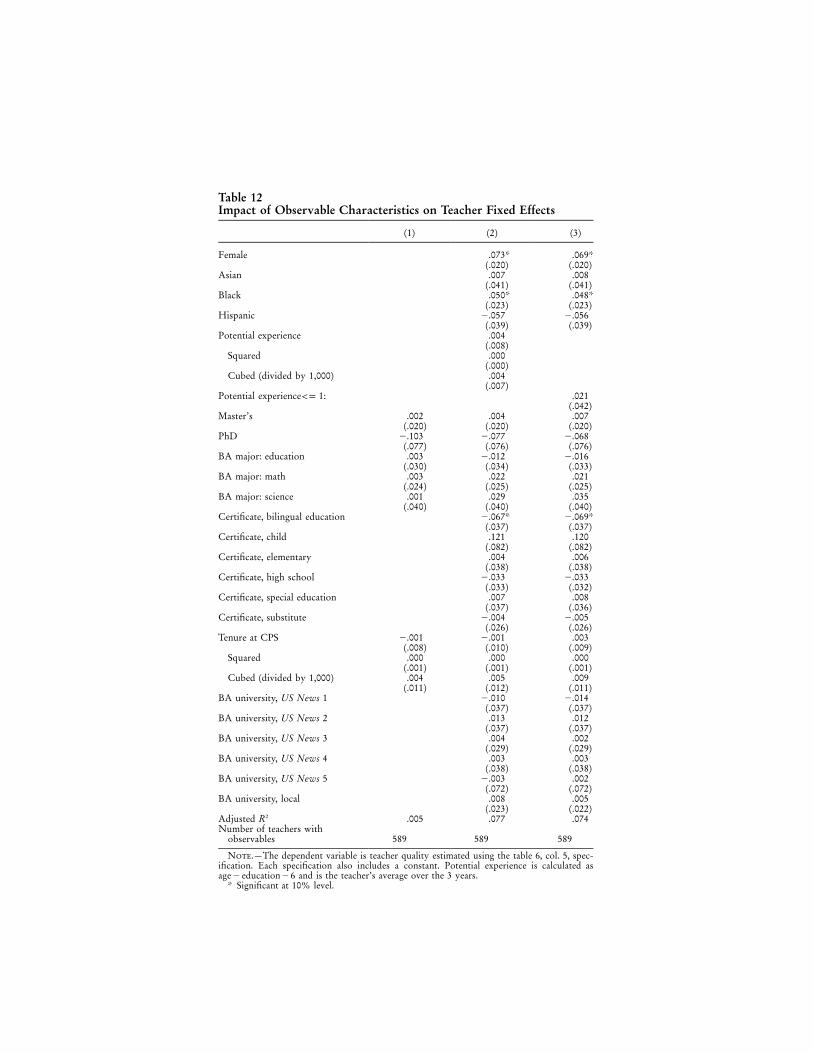
Table 12Impact of Observable Characteristics on Teacher Fixed Effects
(1) (2) (3)
Female .073* .069*(.020) (.020)
Asian .007 .008(.041) (.041)
Black .050* .048*(.023) (.023)
Hispanic �.057 �.056(.039) (.039)
Potential experience .004(.008)
Squared .000(.000)
Cubed (divided by 1,000) .004(.007)
:Potential experience !p 1 .021(.042)
Master’s .002 .004 .007(.020) (.020) (.020)
PhD �.103 �.077 �.068(.077) (.076) (.076)
BA major: education .003 �.012 �.016(.030) (.034) (.033)
BA major: math .003 .022 .021(.024) (.025) (.025)
BA major: science .001 .029 .035(.040) (.040) (.040)
Certificate, bilingual education �.067* �.069*(.037) (.037)
Certificate, child .121 .120(.082) (.082)
Certificate, elementary .004 .006(.038) (.038)
Certificate, high school �.033 �.033(.033) (.032)
Certificate, special education .007 .008(.037) (.036)
Certificate, substitute �.004 �.005(.026) (.026)
Tenure at CPS �.001 �.001 .003(.008) (.010) (.009)
Squared .000 .000 .000(.001) (.001) (.001)
Cubed (divided by 1,000) .004 .005 .009(.011) (.012) (.011)
BA university, US News 1 �.010 �.014(.037) (.037)
BA university, US News 2 .013 .012(.037) (.037)
BA university, US News 3 .004 .002(.029) (.029)
BA university, US News 4 .003 .003(.038) (.038)
BA university, US News 5 �.003 .002(.072) (.072)
BA university, local .008 .005(.023) (.022)
Adjusted R2 .005 .077 .074Number of teachers with
observables 589 589 589
Note.—The dependent variable is teacher quality estimated using the table 6, col. 5, spec-ification. Each specification also includes a constant. Potential experience is calculated as
and is the teacher’s average over the 3 years.age � education� 6* Significant at 10% level.
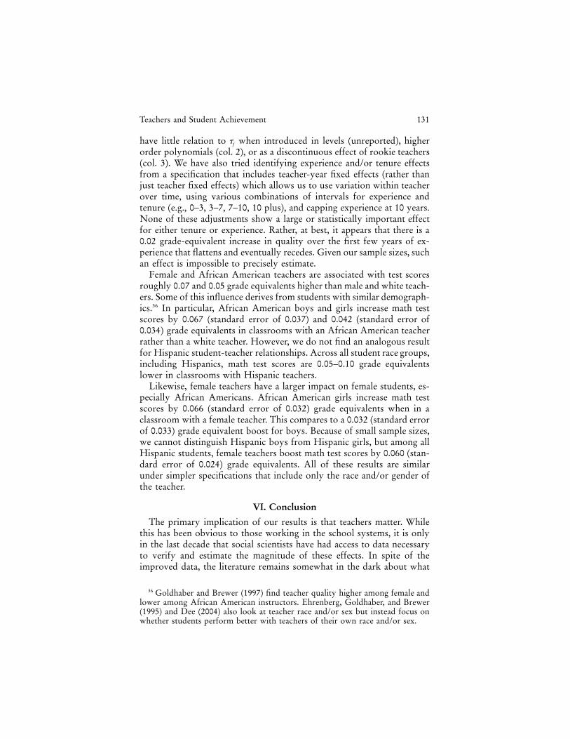
Teachers and Student Achievement 131
have little relation to when introduced in levels (unreported), highertj
order polynomials (col. 2), or as a discontinuous effect of rookie teachers(col. 3). We have also tried identifying experience and/or tenure effectsfrom a specification that includes teacher-year fixed effects (rather thanjust teacher fixed effects) which allows us to use variation within teacherover time, using various combinations of intervals for experience andtenure (e.g., 0–3, 3–7, 7–10, 10 plus), and capping experience at 10 years.None of these adjustments show a large or statistically important effectfor either tenure or experience. Rather, at best, it appears that there is a0.02 grade-equivalent increase in quality over the first few years of ex-perience that flattens and eventually recedes. Given our sample sizes, suchan effect is impossible to precisely estimate.
Female and African American teachers are associated with test scoresroughly 0.07 and 0.05 grade equivalents higher than male and white teach-ers. Some of this influence derives from students with similar demograph-ics.36 In particular, African American boys and girls increase math testscores by 0.067 (standard error of 0.037) and 0.042 (standard error of0.034) grade equivalents in classrooms with an African American teacherrather than a white teacher. However, we do not find an analogous resultfor Hispanic student-teacher relationships. Across all student race groups,including Hispanics, math test scores are 0.05–0.10 grade equivalentslower in classrooms with Hispanic teachers.
Likewise, female teachers have a larger impact on female students, es-pecially African Americans. African American girls increase math testscores by 0.066 (standard error of 0.032) grade equivalents when in aclassroom with a female teacher. This compares to a 0.032 (standard errorof 0.033) grade equivalent boost for boys. Because of small sample sizes,we cannot distinguish Hispanic boys from Hispanic girls, but among allHispanic students, female teachers boost math test scores by 0.060 (stan-dard error of 0.024) grade equivalents. All of these results are similarunder simpler specifications that include only the race and/or gender ofthe teacher.
VI. Conclusion
The primary implication of our results is that teachers matter. Whilethis has been obvious to those working in the school systems, it is onlyin the last decade that social scientists have had access to data necessaryto verify and estimate the magnitude of these effects. In spite of theimproved data, the literature remains somewhat in the dark about what
36 Goldhaber and Brewer (1997) find teacher quality higher among female andlower among African American instructors. Ehrenberg, Goldhaber, and Brewer(1995) and Dee (2004) also look at teacher race and/or sex but instead focus onwhether students perform better with teachers of their own race and/or sex.
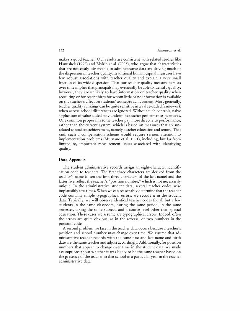
132 Aaronson et al.
makes a good teacher. Our results are consistent with related studies likeHanushek (1992) and Rivkin et al. (2005), who argue that characteristicsthat are not easily observable in administrative data are driving much ofthe dispersion in teacher quality. Traditional human capital measures havefew robust associations with teacher quality and explain a very smallfraction of its wide dispersion. That our teacher quality measure persistsover time implies that principals may eventually be able to identify quality;however, they are unlikely to have information on teacher quality whenrecruiting or for recent hires for whom little or no information is availableon the teacher’s effect on students’ test score achievement. More generally,teacher quality rankings can be quite sensitive in a value-added frameworkwhen across-school differences are ignored. Without such controls, naiveapplication of value added may undermine teacher performance incentives.One common proposal is to tie teacher pay more directly to performance,rather than the current system, which is based on measures that are un-related to student achievement, namely, teacher education and tenure. Thatsaid, such a compensation scheme would require serious attention toimplementation problems (Murnane et al. 1991), including, but far fromlimited to, important measurement issues associated with identifyingquality.
Data Appendix
The student administrative records assign an eight-character identifi-cation code to teachers. The first three characters are derived from theteacher’s name (often the first three characters of the last name) and thelatter five reflect the teacher’s “position number,” which is not necessarilyunique. In the administrative student data, several teacher codes ariseimplausibly few times. When we can reasonably determine that the teachercode contains simple typographical errors, we recode it in the studentdata. Typically, we will observe identical teacher codes for all but a fewstudents in the same classroom, during the same period, in the samesemester, taking the same subject, and a course level other than specialeducation. These cases we assume are typographical errors. Indeed, oftenthe errors are quite obvious, as in the reversal of two numbers in theposition code.
A second problem we face in the teacher data occurs because a teacher’sposition and school number may change over time. We assume that ad-ministrative teacher records with the same first and last name and birthdate are the same teacher and adjust accordingly. Additionally, for positionnumbers that appear to change over time in the student data, we madeassumptions about whether it was likely to be the same teacher based onthe presence of the teacher in that school in a particular year in the teacheradministrative data.
Teachers and Student Achievement 133
Finally, we match students to teachers using a three-letter name codeand the position number for the combinations that are unique in theteacher data.37
References
Abowd, John M., Francis Kramarz, and David Margolis. 1999. High wageworkers and high wage firms. Econometrica 67, no. 2:251–333.
Angrist, Joshua D., and Victor Lavy. 2001. Does teacher training affectpupil learning? Evidence from matched comparisons in Jerusalem pub-lic schools. Journal of Labor Economics 19, no. 2:343–69.
Borjas, George J. 1987. Self-selection and the earnings of immigrants.American Economic Review 77, no. 4:531–53.
Borjas, George J., and Glenn T. Sueyoshi. 1994. A two-stage estimatorfor probit models with structural group effects. Journal of Econometrics64, no. 1–2:165–82.
Clotfelter, Charles T., Helen F. Ladd, and Jacob L. Vigdor. 2004. Teachersorting, teacher shopping, and the assessment of teacher effectiveness.Unpublished manuscript, Public Policy Studies, Duke University.
Coleman, James S., et al. 1966. Equality of educational opportunity. Wash-ington, DC: U.S. Government Printing Office.
Dee, Thomas S. 2004. Teachers, race, and student achievement in a ran-domized experiment. Review of Economics and Statistics 86, no. 1:195–210.
Ehrenberg, Ronald G., Daniel D. Goldhaber, and Dominic J. Brewer.1995. Do teachers’ race, gender, and ethnicity matter? Industrial andLabor Relations Review 48, no. 3:547–61.
Ferguson, Ronald. 1998. Paying for public education. Harvard Journalof Legislation 28:465–98.
Goldhaber, Dan D., and Dominic J. Brewer. 1997. Why don’t school andteachers seem to matter? Journal of Human Resources 32, no. 3:505–23.
Greenwald, Rob, Larry Hedges, and Richard Laine. 1996. The effect ofschool resources on student achievement. Review of Educational Re-search 66:361–96.
Grogger, Jeff, and Eric Eide. 1995. Changes in college skills and the risein the college wage premium. Journal of Human Resources 30, no. 2:280–310.
Hanushek, Eric A. 1971. Teacher characteristics and gains in studentachievement. American Economic Review 61, no. 2:280–88.
———. 1992. The trade-off between child quantity and quality. Journalof Political Economy 100, no. 1:84–117.
37 Note that we assigned some three-letter teacher codes for cases in which theteacher code did not correspond to the first three letters of the teacher’s last name.
134 Aaronson et al.
———. 1996. Measuring investment in education. Journal of EconomicPerspectives 10, no. 4:9–30.
———. 1997. Assessing the effects of school resources on student per-formance: An update. Education Evaluation and Policy Analysis 19:141–64.
———. 2002. Publicly provided education. In Handbook of public fi-nance, vol. 4, ed. Alan Auerbach and Martin Feldstein. Amsterdam:North-Holland Press.
Hanushek, Eric A., and Dennis D. Kimko. 2000. Schooling, labor-forcequality, and the growth of nations. American Economic Review 90, no.5:1184–1208.
Hoxby, Caroline. 2000. Peer effects in the classroom: Learning from gen-der and race variation. Working paper no. 7867, National Bureau ofEconomic Research, Cambridge, MA.
Jacob, Brian A., and Lars Lefgren. 2004. The impact of teacher trainingon student achievement: Quasi-experimental evidence from school re-form efforts in Chicago. Journal of Human Resources 39, no. 1: 50–79.
Jacob, Brian A., and Steven D. Levitt. 2003. Rotten apples: An investi-gation of the prevalence and predictors of teacher cheating. QuarterlyJournal of Economics 118, no. 3:843–77.
Jepsen, Christopher, and Steven Rivkin. 2002. What is the tradeoff be-tween smaller classes and teacher quality? Working paper no. 9205,National Bureau of Economic Research, Cambridge, MA.
Kane, Thomas J., Jonah E. Rockoff, and Douglas O. Staiger. 2006. Whatdoes certification tell us about teacher effectiveness? Evidence fromNew York City. Working paper no. 12155, National Bureau of Eco-nomic Research, Cambridge, MA.
Kane, Thomas J., and Douglas O. Staiger. 2002. The promises and pitfallsof using imprecise school accountability measures. Journal of EconomicPerspectives 16, no. 4:91–114.
———. 2005. Using imperfect information to identify effective teachers.Working paper, Department of Economics, Dartmouth University.
Lazear, Edward. 1999. Personnel economics: Past lessons and future di-rections: Presidential address to the Society of Labor Economists, SanFrancisco, May 1, 1998. Journal of Labor Economics 17, no. 2:199–236.
Manski, Charles F. 1993. Identification of endogenous social effects: Thereflection problem. Review of Economic Studies 60, no. 3:531–42.
Moulton, Brent. 1986. Random group effects and the precision of re-gression estimates. Journal of Econometrics 32:385–97.
Murnane, Richard. 1975. The impact of school resources on the learningof inner city children. Cambridge, MA: Ballinger.
Murnane, Richard, Judith Singer, John Willett, James Kemple, and RandallOlsen. 1991. Who will teach? Policies that matter. Cambridge, MA:Harvard University Press.
Teachers and Student Achievement 135
Rivers, June, and William Sanders. 2002. Teacher quality and equity ineducational opportunity: Findings and policy implications. In Teacherquality, ed. Lance T. Izumi and Williamson M. Evers. Stanford, CA:Hoover Institution Press.
Rivkin, Steven G., Eric A. Hanushek, and John F. Kain. 2005. Teachers,schools, and academic achievement. Econometrica 73, no. 2:417–58.
Rockoff, Jonah E. 2004. The impact of individual teachers on studentachievement: Evidence from panel data. American Economic Review94, no. 2:247–52.
Sacerdote, Bruce. 2001. Peer effects with random assignment: Results forDartmouth roommates. Quarterly Journal of Economics 116, no. 2:681–704.
Summers, Anita A., and Barbara L. Wolfe. 1977. Do schools make adifference? American Economic Review 67, no. 4:639–52.
U.S. Census Bureau. Census 2000, summary file 1. Generated by authorsusing American FactFinder, http://factfinder.census.gov, accessed Oc-tober 23, 2006.
U.S. Department of Education. National Center for Education Statistics.2000. The condition of education 2000. NCES publication no. 2000–062.Washington, DC: U.S. Government Printing Office.
U.S. Department of Education. National Center for Education Statistics.2003. Characteristics of the 100 largest public elementary and secondaryschool districts in the United States: 2001–02. NCES 2003-353, JenniferSable and Beth Aronstamm Young. Washington, DC: U.S. GovernmentPrinting Office.
U.S. News & World Report. 1995. America’s best colleges. Washington,DC: U.S. News & World Report.

Related Documents