A new approach to backward error analysis of LU factorization

BIT 0006-3835/99/3903-0385 $15.001999, Vol. 39, No. 3, pp. 385–402 c© Swets & Zeitlinger

A NEW APPROACH TO BACKWARD ERRORANALYSIS OF LU FACTORIZATION ∗

P. AMODIO and F. MAZZIA†

Dipartimento di Matematica, Universita di Bari, Via E. Orabona 4,

IT-70125 Bari, Italy. email: [email protected]

Abstract.

A new backward error analysis of LU factorization is presented. It allows to obtaina sharper upper bound for the forward error and a new definition of the growth factorthat we compare with the well known Wilkinson growth factor for some classes ofmatrices. Numerical experiments show that the new growth factor is often of orderapproximately log2n whereas Wilkinson’s growth factor is of order n or

√n.

AMS subject classification: 65F05, 65G05.

Key words: Gaussian elimination, stability, backward error analysis, growth factor.

1 Introduction.

Backward error analysis is one of the most powerful tools for studying theaccuracy and stability of numerical algorithms. It was introduced by Wilkinsonin [18] and since then has been extensively used in numerical analysis. A recentsurvey can be found in [13], where a treatment of the behavior of numericalalgorithms in finite precision arithmetic is given. LU factorization was one ofthe first algorithms for which backward error analysis was done.

Wilkinson proved that, in floating point arithmetic, the computed solution xof the n × n linear system Ax = f satisfies

(A + ∆A)x = f ,

where||∆A||∞ ≤ ρW

n p(n)||A||∞ u,(1.1)

p(n) is a cubic polynomial in n, u is the roundoff unit and ρWn is the growth

factor

ρWn =

maxj,i,k |a(j)i,k |

maxi,k |ai,k|.(1.2)

∗Received March 1998. Revised January 1999. Communicated by Robert Schreiber.†Part of this work was performed when the second author was at CERFACS (Centre Eu-

ropeen de Recherche et de Formation Avancee en Calcul Scientifique), France. Work supportedby M.U.R.S.T. (40% project) and by the European Community (Marie Curie–Training andMobility of Researchers, Contract No ERBFMBICT961643).

386 P. AMODIO AND F. MAZZIA

The element a(j)i,k is the computed value in position (i, k) after j steps of factor-

ization. The upper bound (1.1) for the error matrix ∆A is used to obtain theforward error bound

||x − x||∞||x||∞

≤ ρWn p(n)κ(A)u, κ(A) = ||A||∞ ||A−1||∞,(1.3)

even if it is too high. In fact, as Wilkinson notes, for practical purposes thecubic polynomial p(n) can be replaced by a linear polynomial.

Since then, many authors have studied the effect of rounding errors in LUfactorization, with different tools like normwise or componentwise analysis, stat-ing new bounds for the backward and forward errors (see [13] for a completedescription).

Also the growth factor has been extensively analyzed, since it is considered theonly term that may increase the upper bound (1.1). Upper and lower boundsfor ρW

n have been established for certain class of matrices in [4, 5, 9, 10, 13, 17].In [2] a growth factor based on 2-norm has been introduced to show that themaximal growth is achieved by orthogonal matrices.

Following the same approach used in [1] for the cyclic reduction algorithm, inthis paper we present a new backward error analysis for the LU factorization.The upper bound obtained is

||x − x||∞||x||∞

≤ ρnq(n)κ(A)u, ρn =maxj ||Aj ||∞

||A||∞(1.4)

where ρn is a new growth factor based on the ∞-norm (Aj is the computed (n−j)× (n− j) matrix obtained after j steps of factorization). Extensive numericalexperiments show that the new growth factor grows slowly with respect to ρW

n .As an example, for random matrices from the normal distribution ρn grows aslog2n whereas ρW

n grows as√

n.The polynomial q(n) is quadratic in agreement with Wilkinson’s remark that

the cubic polynomial is too high, and this allows us to obtain a sharper upperbound for the forward error. A deeper analysis shows that for M-matrices q(n)is a linear polynomial and for band matrices it depends on the bandwidth.

In this respect this analysis, which exploits the sparsity structure of the er-ror matrices, can be considered as a useful tool for studying the behavior ofalgorithms in finite precision.

2 Block representation of the factorization.

Given an n × n matrix

A =

a1,1 a1,2 · · · a1,n

a2,1 a2,2 · · · a2,n

......

...an,1 an,2 · · · an,n

BACKWARD ERROR ANALYSIS OF LU FACTORIZATION 387

we determine a factorization for A in the form LU in order to solve the linearsystem

Ax = f .(2.1)

We express the factorization of A through n − 1 steps. For simplicity wesuppose that A has already been permuted so that no row pivoting is necessary.Let

A =(

a1 tT1

s1 B1

)

where a1 = a1,1 is scalar, s1 and t1 are vectors of length n− 1 and B1 is a blockof dimension (n−1)× (n−1). The first step of factorization may be representedby

A =(

1a−11 s1 In−1

) (1

A1

) (a1 tT

1

In−1

)= L1D1U1,

where Ij represents the identity matrix of order j and A1 = B1 − a−11 s1tT

1 (A1

is the Schur complement of a1 in A).The second step of the factorization is applied to D1 in order to obtain a

matrix D2 with a sub-block A2 of dimension (n − 2) × (n − 2). In general

Dj−1 =(

Ij−1

Aj−1

)

is factorized in the form

Dj−1 =

Ij−1

1a−1

j sj In−j

Ij−1

1Aj

Ij−1

aj tTj

In−j

= LjDjUj.

After n−1 steps the block An−1 is 1×1 and the factorization ends. The followingsummarizes the factorization of the matrix A:

A = L1 · · ·Ln−1Dn−1Un−1 · · ·U1 =n−1∏j=1

LjDn−1

n−1∏j=1

Un−j .

We now consider a block representation of the LU factorization algorithm forthe solution of the problem (2.1). Letting A0 = A, y0 = f , we introduce thevectors yj and xj of length n − j defined by

xj =(

xj+1

xj+1

), yj =

(y(j)j+1

y∗j

),

where xj+1 and y(j)j+1 are scalars.


Algorithm 2.1.

for j = 1, n − 1vj = a−1

j sj

Aj = Bj − vjtTj

yj = y∗j−1 − y

(j−1)j vj

endxn−1 = A−1

n−1yn−1

for j = n − 1, 1,−1

xj−1 =

(a−1

j (y(j−1)j − tT

j xj)xj

)end

The solution of Ax = f is x0.We denote the elements of vj and Aj in accordance with the usual notation

by

vj =

mj+1,j

...mn,j

, Aj =

a(j)j+1,j+1 · · · a

(j)j+1,n

... · · ·...

a(j)n,j+1 · · · a

(j)n,n

and similarly the elements of yj , xj and tj . The following algorithm is a scalarrepresentation of Algorithm 1.

Algorithm 2.2.

for j = 1, n − 1for i = j + 1, n

mi,j = a(j−1)i,j /a

(j−1)j,j

for k = j + 1, n

a(j)i,k = a

(j−1)i,k − mi,ja

(j−1)j,k

endy(j)i = y

(j−1)i − mi,jy

(j−1)j

endendxn = y

(n−1)n /a

(n−1)n,n

for j = n − 1, 1, −1

xj =(

y(j−1)j −

n∑i=j+1

a(j−1)j,i xi

)/a(j−1)j,j

end

This algorithm is mathematically equivalent to Algorithm 1, but in finite pre-cision the actual rounding errors are usually different. Moreover, they have thesame upper bounds, so it suffices to consider only one of the different implemen-tation of the LU factorization.


3 Analysis of the stability.

For the analysis of the stability we assume that computations are carried outin floating point arithmetic that follows the model

fl(x op y) = (x op y)(1 + u1) or fl(x op y) =x op y

1 + u1, |u1| ≤ u,

where u is the unit round-off and op ∈ {+,−, ∗, /}.The implementation of the LU factorization algorithm on a computer for the

solution of the problem (2.1) gives, instead of the exact solution x, an approxi-mate solution x. In the backward error analysis we obtain an upper bound forthe ∞-norm of the matrix ∆A such that x is the exact solution of the perturbedproblem

(A + ∆A)x = f .

Letting Dj, Lj , Uj be the matrices calculated instead of Dj , Lj and Uj , wedefine

L =n−1∏j=1

Lj and U = Dn−1

n−1∏j=1

Un−j.

Then, letting δA be the matrix containing the error due to the factorization, onehas that

A + δA = LU.(3.1)

Moreover, we consider two further matrices δL and δU containing the error dueto the solution of the triangular systems so that x is the exact solution of thesystem

(L + δL)(U + δU)x = f .

If nu is sufficiently small, the term δL δU is small with respect to the othererror matrices and, in first order approximation, one has

∆A = δA + δL U + L δU(3.2)

while the relative error on the solution may be bounded through [3]

||x − x||||x|| ≤ ||A−1|| ||∆A||.(3.3)

3.1 Stability of the factorization.

To study the stability we use an approach which exploits the sparsity structureof the error matrix δA. The factorization of the matrix A may be expressedthrough a difference equation in matrix form:

D0 = A,

Dj = L−1j Dj−1U

−1j .

In floating point arithmetic

Dj = L−1j Dj−1U

−1j + δDj ,(3.4)


where δDj contains the error at the j-th step of the factorization. In order toevaluate δDj we consider the floating point operations (see the description ofAlgorithm 2.2):

mi,j =(a(j−1)i,j /a

(j−1)j,j

)(1 + ui), i = j + 1, . . . , n,

and

a(j)i,k =

(a(j−1)i,k − mi,j a

(j−1)j,k (1 + u′

i,k))(1 + u′′

i,k), i, k = j + 1, . . . , n,

or in block form (see Algorithm 2.1)

vj = a−1j sj + δvj , Aj = Bj − vj tT

j + δAj

where|δvj | ≤ |a−1

j sj| u, |δAj | ≤ |Bj − vj tTj |u + |vj | |tT

j | u.

Let

Lj =

Ij−1

1vj In−j

, Dj =

Ij−1

1Aj

,

Uj =

Ij−1

aj tTj

In−j

;

then from (3.4) one has

δDj =

Oj−1

0−δvj δvj tT

j − δAj

.

Theorem 3.1. The error matrix δA in (3.1) satisfies

δA =n−1∑j=1

HFj , where HF

j =

Oj−1

0ajδvj δAj

.(3.5)

Proof. To show how the error propagates we define

ε0 = D0 − D0 = A0 − A = 0,

εj = Dj − Dj = L−1j Dj−1U

−1j + δDj − L−1

j Dj−1U−1j .

By adding and subtracting the expressions L−1j Dj−1U

−1j and L−1

j Dj−1U−1j we

obtainεj = L−1

j εj−1U−1j + δDj + (L−1

j − L−1j )Dj−1U

−1j

+ L−1j Dj−1(U−1

j − U−1j ) = L−1

j εj−1U−1j + Zj

(3.6)


where

Zj =

Oj−1

aj a−1j − 1 tT

j − aj a−1j tT

j

δvj + aj a−1j (vj − vj) δAj − δvj tT

j + (vj − vj)(tTj − aj a

−1j tT

j )

.

Solving the difference equation (3.6) one has

εn−1 =n−1∑j=1

n−1−j∏i=1

L−1n−iZj

n−1∏i=j+1

U−1i .

Let Lj =∏j

i=1 Li and Uj =∏j

i=1 Uj−i+1. We multiply both members of theequation to the left for Ln−1 and to the right for Un−1, obtaining

Ln−1(Dn−1 − Dn−1)Un−1 =n−1∑j=1

LjZjUj

and hence

Ln−1Dn−1Un−1 = Ln−1Dn−1Un−1 +n−1∑j=1

LjZjUj

= Ln−1(Dn−1 + Zn−1)Un−1 +n−2∑j=1

LjZjUj .

(3.7)

For what concerns the first term of (3.7) it is easy to see that

Ln−2Ln−1(Dn−1 + Zn−1)Un−1Un−2 = Ln−2Dn−2Un−2 + Ln−2HFn−1Un−2 .

By iterating on Ln−2Dn−2Un−2 and the second term of (3.7), one has

Ln−1Dn−1Un−1 − A = δA =n−1∑j=1

Lj−1HFj Uj−1.(3.8)

The matrix HFj has only a (n− j)× (n− j) block on the main diagonal different

from zero. The matrices Lj−1 and Uj−1 are respectively lower and upper tri-angular and they have the identity matrix in place of the non-null block of HF

j .The result follows by simplifying the expression in (3.8).

In order to obtain an easy upper bound for the norm of δA we consider thegrowth factor

ρn =maxj ||Aj ||∞

||A||∞This factor is slightly different from the usual one defined in (1.2). Nevertheless,it has similar properties, as we shall see in Section 5.


Theorem 3.2. For LU factorization with partial pivoting, the matrices HFj

in (3.5) satisfy

||HFj ||∞ ≤ ||Aj ||∞ u + ||Aj−1||∞ u ≤ 2ρn||A||∞u

and for the error matrix:

||δA||∞ ≤ 2(n − 1)ρn||A||∞ u.(3.9)

Proof. Since |mi,j | ≤ 1,

||HFj ||∞ ≤ max

i

(|a(j−1)

i,j | +n∑

k=j+1

(|a(j)i,k | + |mi,j a

(j−1)j,k |)

)u

≤ maxi

(|a(j−1)

j,j | +n∑

k=j+1

|a(j)i,k | +

n∑k=j+1

|a(j−1)j,k |

)u

≤ ||Aj ||∞ u + ||Aj−1||∞u.

The claim follows from the definition of ρn.Corollary 3.3. If A is a band matrix with lower bandwidth r, then for LU

factorization with partial pivoting one has

||δA||∞ ≤ 2rρn||A||∞ u.

3.2 Stability of the solution of the lower triangular system.

Because of round-off errors, the solution of the lower triangular system gives,instead of the exact solution, an approximate solution y that turns out to bethe exact solution of the problem

(L + δL)y = f .

To calculate δL we introduce, for each Li, an error matrix δLi. From Algo-rithm 2.2 we find that the error at step j derives from

y(j)i =

y(j−1)i − mi,j y

(j−1)j (1 + u′

i)1 + u′′

i

, i = j + 1, . . . , n,

or, in block form,

yj = (In−j + δζj)−1(y∗

j−1 − (vj + δvj)y(j−1)j

)where

|δvj | ≤ |vj | u, |δζj | ≤ In−j u.


Therefore the error matrix at the step j is

δLj =

Oj−1

0δvj δζj

.

To minimize the error in (3.2), we consider the product δL U. One has:Theorem 3.4. The product δL U introduced in (3.2) satisfies

δL U =n−1∑j=1

HLj

where

HLj =

Oj−1

0ajδvj δvj tT

j + δζjAj

.(3.10)

Proof. In first order approximation one hasn−1∏j=1

(Lj + δLj) =n−1∏j=1

Lj +n−1∑j=1

Lj−1δLj

n−1∏i=j+1

Li = L + δL.

Then

δL U =n−1∑j=1

Lj−1δLj

n−1∏i=j+1

LiDn−1

n−1∏i=1

Un−i =n−1∑j=1

Lj−1δLjDjUj .(3.11)

The structure of Lj−1 and Uj allows us to simplify the expression (3.11) and toobtain the following final expression for δL U:

δL U =n−1∑j=1

δLjDjUj,

from which the claim follows easily.The next theorem establishes an upper bound for the infinite norm of δL U.Theorem 3.5. For LU factorization with partial pivoting, the matrices HL

j

in (3.10) satisfy

||HLj ||∞ ≤ (||Aj ||∞ + ||Aj−1||∞)u ≤ 2ρn||A||∞u

and||δL U||∞ ≤ 2(n − 1)ρn||A||∞u.(3.12)

Proof. The proof is analogous to that of Theorem 3.2.Corollary 3.6. If A is a band matrix with lower bandwidth r, then for LU

factorization with partial pivoting one has

||δL U||∞ ≤ 2 rρn||A||∞ u.


3.3 Stability of the solution of the upper triangular system.

By means of a procedure similar to that used in the previous section we cal-culate the matrix δU such that x is the exact solution of

(U + δU)x = y.

The error matrix δU is expressed through a linear combination of δDn−1 andδUj. The error δDn−1 in the last step of the factorization derives from (see thealgorithms in Section 2):

xn =y(n−1)n

a(n−1)n,n (1 + u1)

or xn−1 = (An−1 + δAn−1)−1yn−1

and therefore

δDn−1 =(

On−1

δAn−1

)with |δAn−1| ≤ |An−1| u.

Each δUj may be obtained through

xj =

y(j−1)j −

n∑i=j+1

a(j−1)j,i xi(1 + u′

i)n∏

k=i+1

(1 + u′′k)

a(j−1)j,j (1 + u′

j)(1 + u′′j )

or in matrix form

xj−1 =

((aj + δaj)−1(y(j−1)

j − (tTj + δtT

j )xj)xj

)

with|δaj | ≤ 2 |aj|u, |δtj | ≤ (n − j) |tj |u.

One has

δUj =

Oj−1

δaj δtj

On−j

.

The following theorem gives an expression for L δU.Theorem 3.7. The product L δU in (3.2) satisfies

L δU =n∑

j=1

HUj

where

HUj =

Oj−1

δaj δtTj

δajvj vjδtTj

, j ≤ n − 1,

HUn =

(On−1

δAn−1

).

(3.13)


Proof. In first order approximation:

(Dn−1 + δDn−1)n−1∏j=1

(Un−j + δUn−j)

= Dn−1

n−1∏j=1

Un−j + δDn−1Un−1 + Dn−1

n−1∑j=1

n−1−j∏i=1

Un−iδUjUj−1 = U + δU.

Then

L δU =n−1∏i=1

Li

(δDn−1Un−1 + Dn−1

n−1∑j=1

n−1−j∏i=1

Un−iδUjUj−1

)

= Ln−1δDn−1Un−1 +n−1∑j=1

LjDjδUjUj−1.

(3.14)

Owing to the structure of Lj and Uj−1, we may simplify the expression (3.14)to obtain

L δU = δDn−1 +n−1∑j=1

LjδUj ,

from which the claim follows easily.To determine an upper bound for ||L δU|| , we consider the following:Theorem 3.8. For LU factorization with partial pivoting, the matrices HU

j

in (3.13) satisfy

||HUj ||∞ ≤ (n − j + 1)||Aj−1||∞u ≤ (n − j + 1)ρn||A||∞u

and

||L δU||∞ ≤ n(n + 1)2

ρn||A||∞u.(3.15)

Proof. We consider only the case j < n, since the case j = n is straightfor-ward:

||HUj ||∞ ≤ max

(2|a(j−1)

j,j | + (n − j + 1)n∑

k=j+1

|a(j−1)j,k | ,

maxi>j

(2|a(j−1)

i,j | + (n − j + 1)n∑

k=j+1

|mi,j a(j−1)j,k |

))u

≤ 2|a(j−1)j,j | + (n − j + 1)

n∑k=j+1

|a(j−1)j,k |u

≤ (n − j + 1) ||Aj−1||∞ u.

The claim follows from the definition of ρn.


Corollary 3.9. If A is a band matrix with lower bandwidth r and upperbandwidth s, then for LU factorization with partial pivoting one has

||L δU||∞ ≤ (r + s)rρn ||A||∞ u.

If no pivoting is necessary then

||L δU||∞ ≤ max(2, s)rρn||A||∞ u.

4 Bound for the backward error.

To summarize the results of the backward error analysis made in the previoussections, we calculate the upper bound for the ∞-norm of the error matrix in(3.2). From

||∆A||∞ ≤ ||δA||∞ + ||δL U||∞ + ||L δU||∞and (3.9), (3.12) and (3.15) we obtain

||∆A||∞‖A‖∞

≤(

12n(n + 1) + 4(n − 1)

)ρn u.(4.1)

0 50 100 150 200 250 300 350 400 450 500

10−16

10−14

10−12

10−10

10−8

10−6

Matrix dimension

Back

ward

erro

r

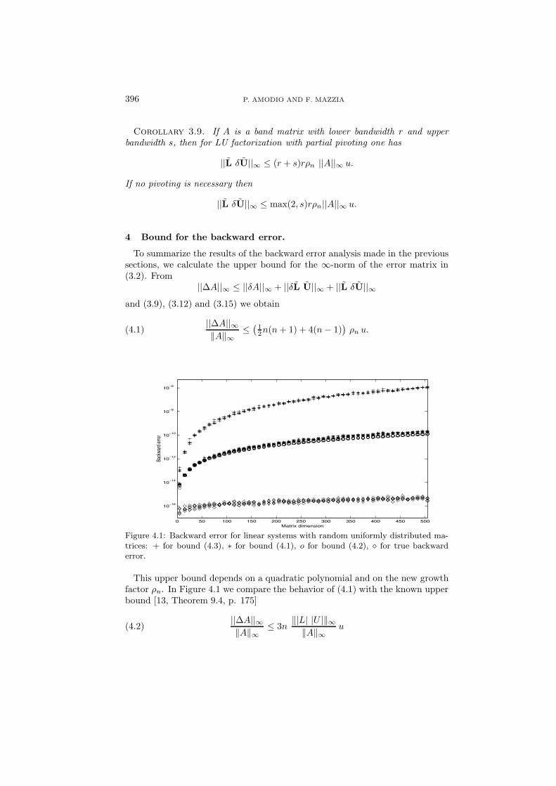
Figure 4.1: Backward error for linear systems with random uniformly distributed ma-trices: + for bound (4.3), ∗ for bound (4.1), o for bound (4.2), � for true backwarderror.

This upper bound depends on a quadratic polynomial and on the new growthfactor ρn. In Figure 4.1 we compare the behavior of (4.1) with the known upperbound [13, Theorem 9.4, p. 175]

||∆A||∞‖A‖∞

≤ 3n‖|L| |U |‖∞

‖A‖∞u(4.2)


where L and U are the triangular matrices of the LU factorization of A, and,since ‖L‖∞ ≤ n and ‖U‖∞ ≤ nρW

n ‖A‖, Wilkinson’s upper bound [13, Theorem9.5, p. 177]

||∆A||∞‖A‖∞

≤ 3n3ρWn u.(4.3)

For each dimension, five random matrices A with normal distributed entries ofmean 0 and standard deviation 1 and random vectors f were generated. Alsorepresented in the figure is the true backward error [7, Theorem 2.2, p. 34]

‖Ax − f‖‖A‖ ‖x‖ .

We note that in this case the behavior of (4.1) is similar to that of (4.2) whilebound (4.3) is much larger. On the other hand, this example emphasizes theusefulness of the new growth factor with respect to the old one. In fact, startingfrom the assumption that ρn grows as ρW

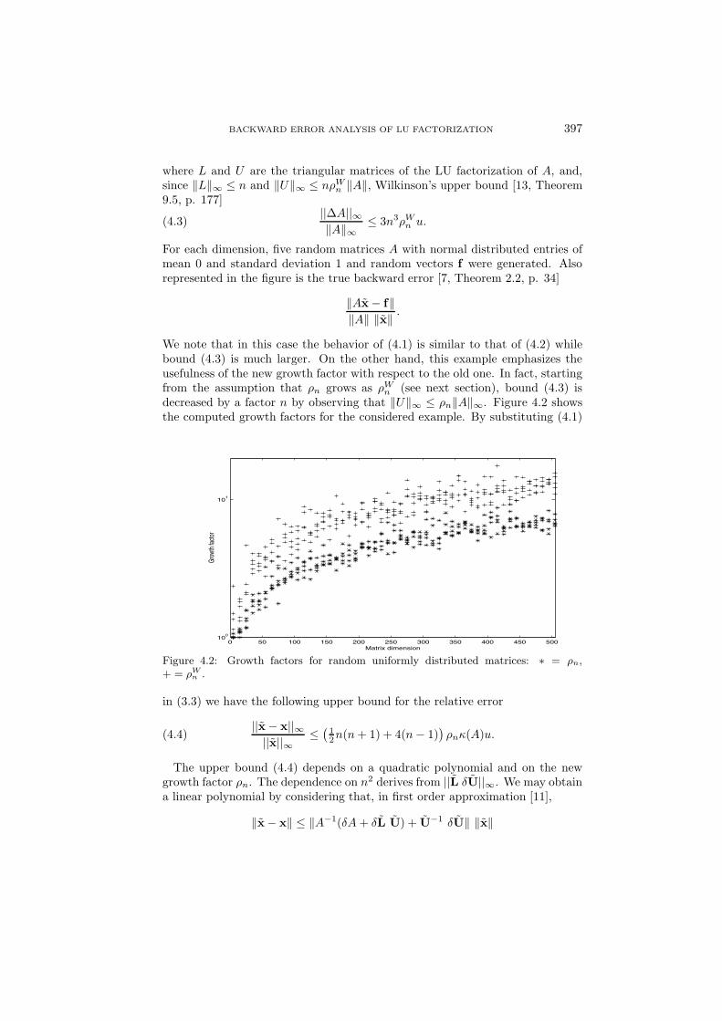
n (see next section), bound (4.3) isdecreased by a factor n by observing that ‖U‖∞ ≤ ρn‖A‖∞. Figure 4.2 showsthe computed growth factors for the considered example. By substituting (4.1)

0 50 100 150 200 250 300 350 400 450 50010

0

101

Matrix dimension

Grow

th fa

ctor

Figure 4.2: Growth factors for random uniformly distributed matrices: ∗ = ρn,+ = ρW

n .

in (3.3) we have the following upper bound for the relative error

||x − x||∞||x||∞

≤(

12n(n + 1) + 4(n − 1)

)ρnκ(A)u.(4.4)

The upper bound (4.4) depends on a quadratic polynomial and on the newgrowth factor ρn. The dependence on n2 derives from ||L δU||∞. We may obtaina linear polynomial by considering that, in first order approximation [11],

‖x− x‖ ≤ ‖A−1(δA + δL U) + U−1 δU‖ ‖x‖


and, since ||δU||∞ ≤ (n − 1) ||U||∞ u,

||x − x||∞||x||∞

≤ (n − 1)(4ρnκ(A) + κ(U)

)u.

As a matter of fact, a bound concerning the matrix U can be substituted by ananalogous concerning the matrix U . In general, the relation between κ(A) andκ(U) is

κ(U) ≤ nρnκ(A).

For an important class of matrices this upper bound does not depend on n.Theorem 4.1. If A is an M-matrix then

κ(U) ≤ ρnκ(A)

and||x − x||∞||x||∞

≤ 5(n − 1)ρnκ(A)u.

Proof. Since A is an M-matrix, A−1 and U−1 are positive, L has non-positiveoff-diagonal elements, and

U−1 = A−1L ≤ A−1,

that is, ||U−1||∞ ≤ ||A−1||∞. Noting that ||U ||∞ ≤ ρn||A||∞ the claim follows.

5 The growth factor.

In the previous section we have introduced a growth factor different from thatdefined by Wilkinson in [18]. A first obvious relation between the two factors is

1n

ρWn ≤ ρn ≤ (n − 1)ρW

n ,

even if the second inequality is too pessimistic and not attainable. Actually,we were not able to find substantial examples where ρn > ρW

n . On the otherhand, to compare effectively the two growth factors, we have computed them fordifferent kinds of matrices that are analysed in [13] and for which a bound forρW

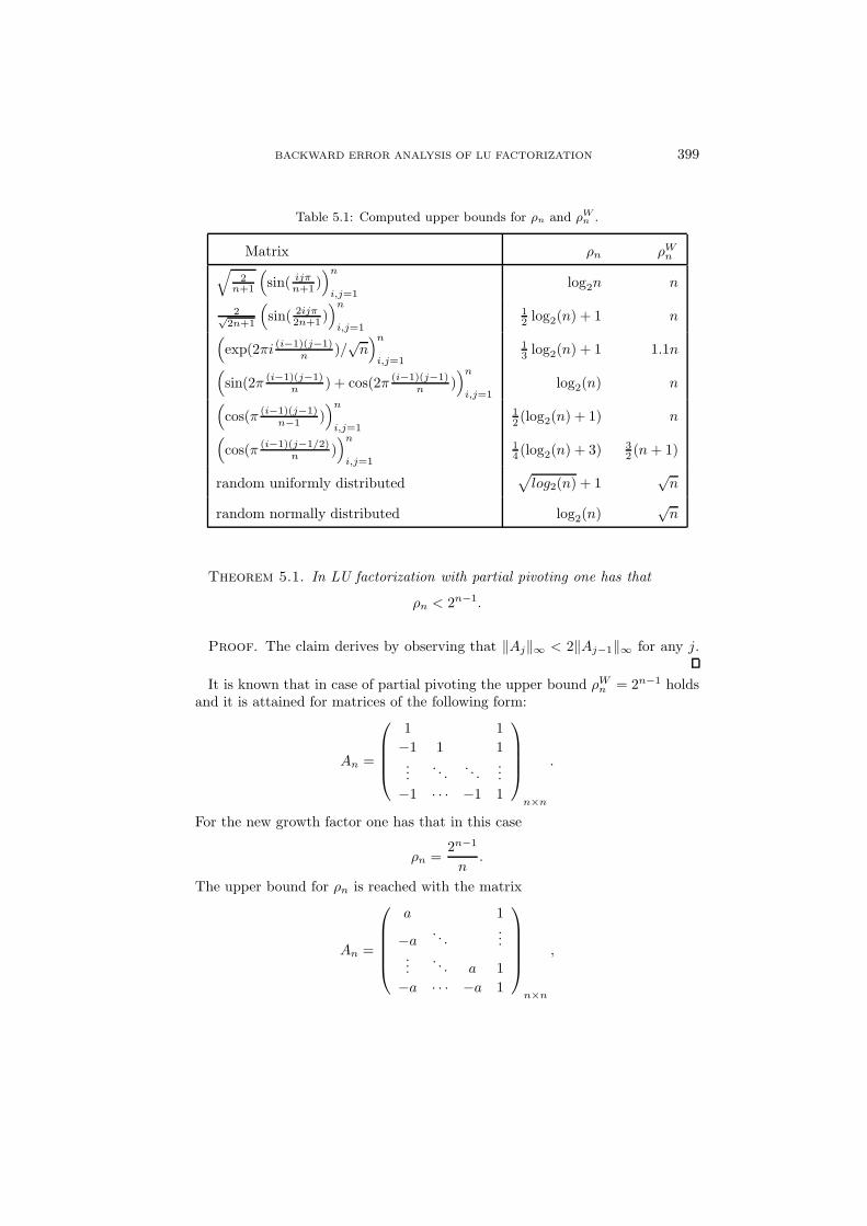
n is known. In Table 5.1 we report the classes of matrices and the computedapproximate behavior of the upper bounds for the two growth factors. Thegeneral conclusion for these classes of matrices is that when ρW

n grows as n, thenew growth factor ρn grows as log2(n) and the bound for the relative error in(4.4) is sharper than the upper bound in (1.3) since, in addition, p(n) is a cubicpolynomial.

The following theorems prove that the two growth factors have similar upperbounds, even if the worst case for ρn is not attainable. To avoid bounds involvingunit roundoff, we use the following formula:

ρn =maxj ‖Aj‖∞

‖A‖∞.

However, the same is usually done for ρWn (see [13, p. 177]).


Table 5.1: Computed upper bounds for ρn and ρWn .

Matrix ρn ρWn√

2n+1

(sin( ijπ

n+1 ))n

i,j=1log2n n

2√2n+1

(sin( 2ijπ

2n+1 ))n

i,j=1

12 log2(n) + 1 n(

exp(2πi (i−1)(j−1)n )/

√n)n

i,j=1

13 log2(n) + 1 1.1n(

sin(2π (i−1)(j−1)n ) + cos(2π (i−1)(j−1)

n ))n

i,j=1log2(n) n(

cos(π (i−1)(j−1)n−1 )

)n

i,j=1

12 (log2(n) + 1) n(

cos(π (i−1)(j−1/2)n )

)n

i,j=1

14 (log2(n) + 3) 3

2 (n + 1)

random uniformly distributed√

log2(n) + 1√

n

random normally distributed log2(n)√

n

Theorem 5.1. In LU factorization with partial pivoting one has that

ρn < 2n−1.

Proof. The claim derives by observing that ‖Aj‖∞ < 2‖Aj−1‖∞ for any j.

It is known that in case of partial pivoting the upper bound ρWn = 2n−1 holds

and it is attained for matrices of the following form:

An =

1 1−1 1 1...

. . . . . ....

−1 · · · −1 1

n×n

.

For the new growth factor one has that in this case

ρn =2n−1

n.

The upper bound for ρn is reached with the matrix

An =

a 1

−a. . .

......

. . . a 1−a · · · −a 1

n×n

,


by choosing a = 1n(n−1) . In this case

ρn =2n−1

1 + 1/n.

For matrices with some special properties or structures, we can say somethingmore about the behavior of the growth factor. In the following theorems weconsider diagonally dominant and Hessenberg matrices.

Theorem 5.2. If A is diagonally dominant by rows, then

ρn ≤ 1.

Proof. The claim follows from the following Lemmas 5.3 and 5.4. The proofof both Lemmas is straightforward.

Lemma 5.3. If A0 = A is diagonally dominant, then all the matrices Aj arediagonally dominant.

Lemma 5.4. If A is diagonally dominant by rows, then, for each matrix Aj,one has that

||Aj ||∞ ≤ ||A||∞.

0 100 200 300 400 500 600 700 80010

0

101

102

103

Matrix dimension

Grow

th fa

ctor

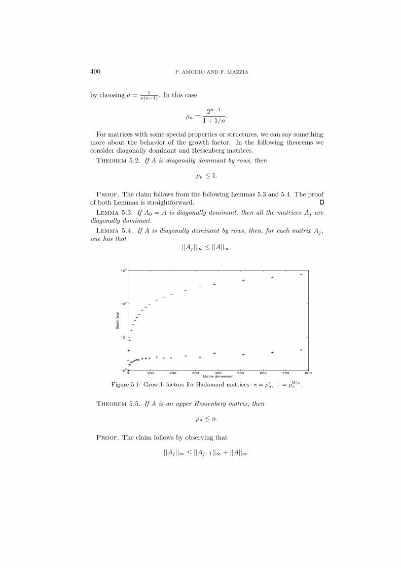
Figure 5.1: Growth factors for Hadamard matrices: ∗ = ρcn, + = ρW,c

n .

Theorem 5.5. If A is an upper Hessenberg matrix, then

ρn ≤ n.

Proof. The claim follows by observing that

||Aj ||∞ ≤ ||Aj−1||∞ + ||A||∞.


We prove this inequality by induction. For a generic matrix Aj one has

n∑k=j+1

|a(j−1)i,k − mi,ja

(j−1)j,k | ≤

n∑k=j+1

|a(j−1)i,k | +

n∑k=j+1

|a(j−1)j,k |(5.1)

and since the matrix is upper Hessenberg, one of the sums in the right-hand sideof (5.1) involves elements of the matrix A.

Concerning the complete pivoting, most of the results about the growth factorare reported by Higham [10], which gives a lower bound for ρW,c

n and evaluatesit for Hadamard and orthogonal matrices.

We report in Figure 5.1 the computed growth factors ρW,cn (dashed line) and ρc

n

(dash-dotted line) for Hadamard matrices. We observe that ρcn grows as log2(n)

while ρW,cn grows as n.

Acknowledgements.

The authors would like to acknowledge Prof. D. Trigiante for fruitful discus-sions and comments, and S. Gratton for useful suggestions. They are also verygrateful to one anonymous referee which greatly improved the readability of themanuscript.

REFERENCES

1. P. Amodio and F. Mazzia, Backward error analysis of cyclic reduction for the so-lution of tridiagonal linear systems, Math. Comp., 62 (1994), pp. 601–617.

2. J. L. Barlow and H. Zha, Growth in Gaussian elimination, orthogonal matrices,and two-norm, SIAM J. Matrix Anal. Appl., 19 (1998), pp. 807–815.

3. A. K. Cline, C. B. Moler, G. W. Stewart, and J. H. Wilkinson, An estimate for thecondition number of a matrix, SIAM J. Numer. Anal., 16 (1979), pp. 368–375.

4. C. W. Cryer, Pivot size in Gaussian elimination, Numer. Math., 12 (1968), pp. 335–345.

5. J. Day and B. Peterson, Growth in Gaussian elimination, Amer. Math. Monthly,(1988), pp. 489–513.

6. C. de Boor and A. Pinkus, Backward error analysis for totally positive linear sys-tems, Numer. Math., 27 (1977), pp. 485–490.

7. J. W. Demmel, Applied Numerical Linear Algebra, SIAM, Philadelphia, 1997.

8. G. H. Golub and C. F. Van Loan, Matrix Computations, 3rd ed., Johns HopkinsUniversity Press, Baltimore, 1996.

9. N. Gould, On growth in Gaussian elimination with complete pivoting, SIAM J.Matrix Anal. Appl., 12 (1991), pp. 354–361.

10. N. J. Higham and D. J. Higham, Large growth factors in Gaussian elimination withpivoting, SIAM J. Matrix Anal. Appl., 10 (1989), pp. 155–164.

11. N. J. Higham, The accuracy of solutions to triangular systems, SIAM J. Numer.Anal., 26 (1989), pp. 1252–1265.

12. N. J. Higham, Bounding the error in Gaussian elimination for tridiagonal systems,SIAM J. Matrix Anal. Appl., 11 (1990), pp. 521–530.


13. N. J. Higham, Accuracy and Stability of Numerical Algorithms, SIAM, Philadelphia,1996.

14. V. Lakshmikantham and D. Trigiante, Theory of Difference Equations: NumericalMethods and Applications, Academic Press, New York, 1988.

15. R. D. Skeel, Scaling for numerical stability in Gaussian elimination, J. Assoc. Com-put. Mach., 26 (1979), pp. 494–526.

16. R. D. Skeel, Iterative refinement implies numerical stability for Gaussian elimina-tion, Math. Comp., 35 (1980), pp. 817–832.

17. L. N. Trefethen and R. S. Schreiber, Average-case stability of Gaussian elimination,SIAM J. Matrix Anal. Appl., 11 (1990), pp. 335–360.

18. J. H. Wilkinson, The Algebraic Eigenvalue Problem, Oxford University Press, Ox-ford, 1965.

A new approach to backward error analysis of LU factorization

Documents