A Neural Lyapunov Approach to Transient Stability ...

A Neural Lyapunov Approach to Transient Stability Assessment inInterconnected Microgrids

Tong HuangTexas A&M [email protected]

Sicun GaoUniversity of California,

San [email protected]

Xun LongDelta Electronics (Americas)

[email protected]

Le XieTexas A&M University

[email protected] ∗

Abstract

We propose a neural Lyapunov approachto assessing transient stability in powerelectronic-interfaced microgrid interconnections.The problem of transient stability assessment is cast asone of learning a neural network-structured Lyapunovfunction in the state space. Based on the functionlearned, a security region is estimated for monitoringthe security of interconnected microgrids in real-timeoperation. The efficacy of the approach is testedand validated in a grid-connected microgrid and athree-microgrid interconnection. A comparison studysuggests that the proposed method can achieve a lessconservative characterization of the security region, ascompared with a conventional approach [1].

1. Introduction

Microgrids provide promising solutions toenhancing the resiliency of distribution systemswith increasing level of penetration of distributedenergy resources (DERs) [2–5]. The flexibility ofmicrogrids is enabled by their two operation modes:an islanded mode and a grid-connected mode [6]. Inthe grid-connected mode, one microgrid interconnectswith the rest of the distribution system via the pointof common coupling (PCC) [6] in order to achieveentire system-wide optimal operation. A microgrid isalso capable of proactively transitioning to an islandedmode, once the main grid loses its desirable functions orsevere faults in the microgrid compromise the securityof the main grid [3, 4].

The control and management of grid-connectedmicrogrids is typically hierarchically structured [6–8]. At the individual microgrid level, a microgridcentral controller (MGCC) regulates the interconnecteddistributed generation units (DGUs) by tuning thesetpoints of their local controllers [2, 6, 7]. At∗The work of T. Huang and L. Xie is supported in part by NSF

ECCS-1611301, 2038963, and DOE grant DE-EE0009031.

the distribution-system level, a distribution systemoperator (DSO) coordinates interconnected microgridsby controlling microgrid interfaces, rather than directlyregulating DGUs [2]. Voltage source inverters (VSI)generally serve as the interfaces of microgrids, wherevarious control strategies, such as master/slave, currentsharing, and frequency/angle droop methods [2,7,8], canbe implemented.

The rise of interest in deploying microgrids andinterconnection of multiple microgrids provides manyresearch challenges and opportunities in the designand operation of their energy management systems.One particular area of challenge is how to design safeand efficient transient stability assessment tools forfuture grid designers and operators. Transient stabilityassessment for microgrids essentially aims to answerthe following question: Given an operating condition, towhat extent of disturbances can the microgrids tolerate?A rigorous answer to such a question is much needed forboth offline design and online operation of microgrids.For example, the stability assessment tool providesmicrogrids’ designers with a criterion for optimal designscheme selection. Such an assessment tool also allowsDSO to maintain greater situational awareness and helpsthem to decide if corrective actions need be taken afterdisturbances happen. The challenge of developing suchan assessment tool lies in the fact that microgrids andtheir interconnections are nonlinear systems [2, 6] andthe dynamics of such nonlinear systems under largedisturbances need be analyzed.

In view of the above challenge, severaltechniques are proposed for stability assessmentin both the microgrid level [6, 9–11] and themicrogrid-interconnection level [2, 4, 12–14]. Thispaper focuses on the level of interconnected microgrids.Within such a research scope, one possible method is toleverage the energy function approach that is extensivelystudied in analysis of large-scale transmission systems.By assuming that the transmission lines are lossless,the energy function approach constructs a systembehavior-summary function, namely, the energy

Proceedings of the 54th Hawaii International Conference on System Sciences | 2021

Page 3330URI: https://hdl.handle.net/10125/71020978-0-9981331-4-0(CC BY-NC-ND 4.0)

function, in order to certify the stability of a equilibriumpoint. Reference [15] provides a thorough surveyfor the energy function approach in transmissionsystems. However, the qualitative difference betweentransmission systems and interconnected microgridsmay prevent the energy approach developed fortransmission systems to migrate to interconnectedmicrogrids. For example, the lossless-line assumptionis a valid assumption for transmission systems, butdistribution lines in interconnected microgrids have alower reactance to resistance ratio in comparison withtransmission systems [6], rendering the lossless-lineassumption invalid and, thereby, leading to thenonexistence of the energy function [1]. Withoutthe lossless-line assumption, reference [2] decouplesthe slow and fast dynamics in the interconnectedmicrogrid and analyzes them separately: The stabilityof slow dynamics is addressed by the linearizationtechnique [16] widely applied in bulk transmissionsystem applications [17–20]; and the transient stabilityof fast dynamics is assessed by linear matrix inequality(LMI). However, the proposed framework in [2] onlyprovides a binary (yes/no) answer to transient stabilityof the interconnected microgrids. It is equally importantto estimate the extent of disturbances that can betolerated by interconnected microgrids.

This paper leverages the most recent advancesin machine learning and control theory to providerigorious and scalable assessment of transient stabilityin interconnected microgrids. A neural Lyapunovapproach is proposed for assessing transient stabilityof a microgrid interconnection. The problem oftransient stability assessment is cast as one of learninga neural network-structured Lyapunov function inthe state space. Based on the function learned,a security region is estimated for monitoring thesecurity of interconnected microgrids in real-timeoperation. The contribution of this paper is twofold:1) It introduces a novel type of Lyapunov functionthat can rigorously establish asymptotic stability ofinterconnected microgrids and provide a securityregion that allows microgrids’ designers/operators toestimate the extent of disturbances that a microgridinterconnection can tolerate; and 2) the proposedapproach does not require a special form of interfacedynamics of interconnected microgrids, allowing it toanalyzing realistic microgrid interconnections.

The rest of this paper is organized as follows:Section 2 presents the mathematical descriptionof interconnected microgrid dynamics; Section3 elaborates procedures for learning a neuralnetwork-structured Lyapunov function and findinga security region by the Lyapunov function learned;

Section 4 tests and validates the proposed approach; andSection 5 concludes the paper and points out the futuredirection of this work.

2. Dynamics of Networked Microgrids

A future distribution system can be consideredas an interconnection of m PE-interfaced microgrids.For microgrid i ∈ {1, 2, . . . ,m}, its PCC interfacedynamics can be described by the following differentialequations: [2, 4]

TAiδi = DAi(P∗i − Pi)− (δi − δ∗i ) (1a)

TEiEi = DEi(Q∗i −Qi)− (Ei − E∗i ), (1b)

where state variables δi and Ei are the voltage angleand voltage magnitude at the i-th PCC, respectively;algebraic variables Pi andQi are real and reactive powerinjections to the i-th PCC; setpoints δ∗i , E∗i , P ∗i , andQ∗i are dispatched by a distribution system operatorbased on steady-state security/economic studies; controlparameters TAi and TEi denote tracking time constantsof voltage angle and magnitude at PCC i; and DAi andDEi are droop gains of voltage angle and magnitudeat PCC i [2, 4]. Note that equation (1) describesthe interface dynamics with angle droop control. Ifthe frequency droop control is deployed in microgridinterfaces, the swing-equation type of dynamics willreplace (1).

Microgrid i is interconnected with other microgridsthrough distribution lines which introduce the followingalgebraic constrains:

Pi = E2iGii +

∑k 6=i

EiEkYik cos(δi − δk − θik), (2a)

Qi = −E2iBii +

∑k 6=i

EiEkYik sin(δi − δk − θik),∀i,

(2b)

where Yik∠θik denotes the element at the i-th rowand the k-th column of admittance matrix Y ; Giiand Bii are real and imaginary parts of Yii∠θii,respectively. Suppose that the equilibrium point of them-microgrid interconnection described by differentialalgebraic equations (DAEs) (1) and (2) is

o = [δ∗1 , δ∗2 , . . . , δ

∗m, E

∗1 , E

∗2 , . . . , E

∗m]> (3)

where variables δ∗i and E∗i for all i ∈ 1, 2, . . . ,m satisfy

Page 3331

P ∗i = E∗2i Gii +∑k 6=i

E∗i E∗kYik cos(δ∗i − δ∗k − θik),

(4a)

Q∗i = −E∗2i Bii +∑k 6=i

E∗i E∗kYik sin(δ∗i − δ∗k − θik),∀i.

(4b)

Next we modify (1) and (2) such that the equilibriumpoint of the modified DAEs is the origin of the statespace. Define new state variables

δ′i = δi − δ∗i , (5a)E′i = Ei − E∗i ,∀i. (5b)

With new state variables δ′i and E′i, the i-th PCCinterface dynamics is characterized by differentialequations

TAiδ′i = DAi(P∗i − Pi)− δ′i (6a)

TEiE′i = DEi(Q∗i −Qi)− E′i, (6b)

with algebraic equations

Pi = (E′i + E∗i )2Gii+∑k 6=i

(E′i + E∗i )(E′k + E∗k)Yik cos(δ′ik + δ∗ik − θik),

(7a)

Qi = −(E′i + E∗i )2Bii+∑k 6=i

(E′i + E∗i )(E′k + E∗k)Yik sin(δ′ik + δ∗ik − θik),∀i,

(7b)

where δ′ik = δ′i−δ′k and δ∗ik = δ∗i −δ∗k. The equilibriumpoint of the dynamic system described by (6) and (7) isthe origin of the state space.

It is worth noting that if time constant TEi is muchgreater than TAi, the evolution of δ′i is much faster thanthat of E′i. Therefore, when phase angles are the statevariables of interest, E′i in (6) can be assumed to be aconstant [2], i.e., E′i = 0. Such an assumption is calledthe time-scale separation assumption [4]. Under thetime-scale separation assumption, the system equations(6) and (7) can be simplified to

TAiδ′i = DAi(P∗i − Pi)− δ′i,∀i, (8)

where

Pi = E∗2i Gii +∑k 6=i

E∗i E∗kYik cos(δ′ik + δ∗ik − θik).

(9)

The system equations (6) or (8) can be written in thefollowing compact form:

x = f(x) (10)

where f(·) corresponds to (8) if TEi � TAi, otherwise itassociates with (6); and the state vector x is defined by

x :=

{[δ′1, δ

′2, . . . , δ

′m]> TEi � TAi

[δ′1, δ′2, . . . , δ

′m, E

′1, E

′2, . . . , E

′m]> otherwise.

(11)The equilibrium point o′ of (10) is an m′-dimensionalzero vector, i.e., o′ = 0m′ , wherem′ = m if TEi � TAi,otherwise m′ = 2m.

For the interconnected microgrids described by (10),it is highly desirable for microgrids’ designers/operatorsto know: 1) whether the equilibrium point o′ isasymptotically stable; and 2) how much state deviationfrom o′ (caused by disturbances, say, line tripping) theinterconnected microgrids can tolerate.

3. Transient Stability Assessment

This section presents a neural Lyapunov approachto transient stability assessment in the PE-interfacedmicrogrid interconnection described by (10). First,some background knowledge is presented in order toshow that one possible way to answer the two questionsraised at the end of Section 2 is to construct a Lyapunovfunction. Then the Lyapunov function is learnedby minimizing the empirical Lyapunov risk [21] andaugmenting training samples. Finally, a region ofattraction is estimated based on the Lyapunov functionlearned.

3.1. Background Definitions

We consider the interconnected microgridsdescribed by (10) with the equilibrium point o′ atthe origin. A Lyapunov function [22] can be leveragedto establish the stability of the equilibrium point o′ andits definition is as follows:Definition 1 If, in a ball DR := {x|‖x‖22 ≤ R2}, thereexists a continuous differentiable scalar function V suchthat

• V is positive definite in DR,

• V is negative definite in DR

then the equilibrium point o′ is asymptotically stable,and the function V is called a Lyapunov function.

In Definition 1, a positive/negative definite functionin DR is defined as follows. A function F (x) is a

Page 3332

positive definite function in DR, if F (0) = 0 andF (x) > 0 for all x ∈ DR \ {0}. A function F (x) is anegative definite function in DR, if −F (x) is a positivedefinite function in DR. V (x) is the time derivative ofV (x) and it can be found by

V =dV (x)

dt=∂V

∂xf(x). (12)

Definition 1 essentially suggests that we can answerthe first question raised at the end of Section 2 bysearching for a legitimate Lyapunov function V (x):the asymptotic stability can be certified, if a Lyapunovfunction can be found.

We proceed to address the second question at theend of Section 2, viz., how much state deviation fromo′ the interconnected microgrids can tolerate. Such aquestion boils down to finding a region in the state spacesuch that the system trajectory initiating from the regionnever leaves the region and converges to the origin ofthe state space [21, 22]. In this paper, such a region iscalled a security region R, which is formally defined asfollows:Definition 2 A regionR ⊆ Rm′ is a security region if

x(0) ∈ R =⇒ x(∞) = 0m′ ∧ ∀t > 0(x(t) ∈ R).

In Definition 2, 0m′ is an m′-dimension zero vector;and “∧” means “and.” Based on Definition 2, a securityregion is a subset of the domain of attraction [22]. If aLyapunov function V (x) is available, one estimation forthe security regionR is

Rc = {x ∈ DR|c ∈ R+, V (x) < c}. (13)

The security region estimation Rc can be leveragedfor online stability assessment for interconnectedmicrogrids: if the state deviation from thepre-dispatched equilibrium o′ falls within Rc, thesystem is guaranteed to be secure, as state deviationsnever leaveRc and tend to zeros as time goes to infinity.

Definition 1 and equation (13) can be used to 1)certify the asymptotic stability and 2) estimate a securityregion around an equilibrium point dispatched by DSO.However, the prerequisite to achieve the above two goalis the availability of a Lyapunov function. In whatfollows we present how to find such a function usingneural network.

3.2. Neural Network-structured LyapunovFunction

We assume that the Lyapunov function V (x) has aneural-network structure, as such a structure enables us

to approximate a wide class of functions. The inputof the neural network is state vector x, and the outputis the value of V evaluated at x. The fundamentalcomputing units of the neural-network are neuronswhich is a multiple-input-single-output system [23–25].Suppose that the input of the neuron i is x0. Neuron iconducts a two-step computing procedure. First, neuroni takes linear combination of its input and obtain anintermediate variable di, i.e.,

di = wix0 + bi (14)

where wi ∈ R1×|x0| collects weighting coefficients; andbi ∈ R is a bias coefficient. Second, neuron i evaluates anonlinear function (a.k.a. the activation function) at x0

and returns the function value as its output y0. In thispaper, the hyperbolic tangent function is chosen to bethe activation function, i.e.,

yi = tanh(di). (15)

The neurons are interconnected in a layered architectureand constitute a neural network. A neural networkcomprises an input layer, at least one hidden layer, andan output layers. This paper uses a neural network withone hidden layer to approximate the Lyapunov functionV (x).

We proceed to analyze the neurons in the hiddenlayer. Let d[1] collect all intermediate variables ofneurons in the hidden layer, i.e.,

d[1] := [d[1]1 , d

[1]2 , . . . , d

[1]nH

]> (16)

where d[1]i denotes the intermediate variable of the i-thneuron in the first layer, viz., the only hidden layer;and nH is the number of neurons in the hidden layer.Similarly, define y[1] by

y[1] := [y[1]1 , y

[1]2 , . . . , y[1]nH

]> (17)

where y[1]i denotes the output of the i-th neuron in thefirst layer. The two-step procedure of neurons in thehidden layer leads to

d[1] = W [1]x + b[1] (18a)

y[1] = tanh(d[1]) (18b)

whereW [1] := [w[1]j,k] collects the weighting coefficients

of the neurons in the hidden layer, whence its (j, k)-thentry is the weighting coefficient for the k-th input ofthe j-th neuron; column vector b[1] ∈ RnH collectsbias coefficients; and tanh denotes the element-wisedhyperbolic tangent function.

Page 3333

Following the similar notation system, for the outputlayer, we have

d[2] = W [2]y[1] + b[2] (19a)

y[2] = tanh(d[2])

(19b)

where d[2] and b[2] are the intermediate variable and biascoefficient vector of the neuron at the second (output)layer, respectively; W [2] ∈ R1×nH collects weightingcoefficients of the neuron at the output layer; and y[2] ∈R is the output of the neural network.

Let a vector α collect all unknown parameters inW [1],W [2], b[1], and b[2]. One can randomly draw nstate vectors x1, x2, . . ., xn from the state space andevaluate output of the neural network with parametersα. These state vectors can be considered as trainingexamples for the neural network. A key question ishow to tune parameters α such that the neural networkrepresented by (18) and (19) behaves like a Lyapunovfunction. Such a question is addressed by introducing acost function in the following sections.

3.3. Empirical Lyapunov Risk

In order to enable the neural network described by(18) and (19) to behave like a Lyapunov function, thefollowing cost function, i.e., empirical Lyapunov risk, isintroduced to update parameters α:

Ln,ρ(α) =1

n

n∑k=1

max (0,−Vα(xk))+

1

n

n∑k=1

max(0, Vα(xk))

(20)

where n is the number of training examples; and ρis the probability distribution according to which thetraining examples are drawn. If Vα is not a legitimateLyapunov function, positive penalties can be incurred inthe the cost function Ln,ρ(α). The parameters α∗ ofa legitimate Lyapunov function can minimize the costfunction Ln,ρ(α). The cost function (20) is called theLyapunov risk in [21]. In practice, the “max” functionin (20) can be replaced by the Rectified Linear Unit(ReLU) which is defined by

ReLU(z) =

{z z ≥ 0

0 z < 0.(21)

Equation (20) is equivalent to

Ln,ρ(α) =1

n

n∑k=1

(ReLU(−Vα(xk)) + ReLU(Vα(xk))

).

(22)Besides, Vα can be evaluated by (12), viz.,

Vα =∂Vα∂x

f(x). (23)

Since the Lyapunov function candidate Vα (= y[2]) hasa neural-network structure,

(∂Vα

∂x

)can be expressed in

terms of the parameters in set α according to the chainrule:

∂Vα∂x

=∂Vα∂d[2]

∂d[2]

∂y[1]

∂y[1]

∂d[1]

∂d[1]

∂x. (24)

In (24),

∂Vα∂d[2]

= 1− V 2α,

∂d[2]

∂y[1]= W [2],

∂d[1]

∂x= W [1],

∂y[1]

∂d[1]= diag

(1− tanh2(d

[1]1 ), . . . , 1− tanh2(d[1]nH

)),

where

d[1]k = W

[1]k,:x + b

[1]k , k = 1, 2, . . . , nH.

whence W [1]k,: denotes the k-th row of matrix W [1]; and

b[1]k is the k-th entry of b[1].

Suppose that we have a training set X with n i.i.d.examples randomly drawn from the state space, i.e.,

X := {x1,x2, . . . ,xk, . . . ,xn} (26)

where xk ∼ ρ for k = 1, 2, . . . , n. Based onthe training set X , one can find the coefficients of aneural network-structured Lyapunov function candidateby minimizing the Lyapunov risk, i.e.,

minαLn,ρ(α). (27)

The optimization problem (27) can be solved by thestochastic gradient decent method. The pseudo-code ofthe method is presented in Algorithm 1 where α0 is theinitial guess of the parameters; and η is the learning ratespecified by users.

3.4. Training Set Augment

The Lyapunov function candidate with parameters αthat is returned by Algorithm 1 may not be a legitimate

Page 3334

Algorithm 1 Learning Lyapunov Function Candidate1: function Learning(X ,α0, η, f , nH)2: α← α0

3: for x ∈ X do4: Compute Vα and Vα via (18), (19), (12)5: Evaluate L|X |,ρ(α) through (22)6: α← α− η∇αL|X |,ρ(α)7: end for8: return α.9: end function

Lyapunov function. The reason is that the function withα might violate the two conditions in Definition 1 whenit is evaluated at the training examples that are not inX . Therefore, it is necessary to find counterexamplesthat lead the candidate function Vα∗ to violate the twoconditions in Definition 1 and add the counterexamplesto the training set X .

Recent advances in satisfiability modulo theories(SMT) can be leveraged to find the counterexamples.The SMT solver finds the counterexamples by checkingthe satisfiability of the following condition:(

‖x‖22 ≥ r2)∧(Vα(x) ≤ 0 ∨ Vα(x) ≥ 0

)(28)

where x ∈ DR; r � min(1, ‖x‖2) and “∨” denotes

“or”. The condition ‖x‖22 ≥ r2 is added for avoidingnumerical issues [21]. The SMT solver, such as dReal[26], can return a set S that comprises some x satisfyingcondition (28). If no x can be found in DR, S is anempty set. Such a procedure is presented in Algorithm2. Algorithm 3 shows the overall procedure to find alegitimate Lyapunov function.

Algorithm 2 Training Set Augment1: function AugSet(Vα, f , r, R,X )2: γ ← 13: Check (28) and find S via SMT solver4: if S 6= Ø then5: X ← X ∪ S6: else7: γ = 08: end if9: return γ, X .

10: end function

3.5. Security Region Estimation

Given the neural network-structured Lyapunovfunction Vα∗ learned from the state space, a security

Algorithm 3 Lyapunov Neural Network1: inputs: X ,α0, η, nH, f , r, R2: γ ← 13: while γ = 1 do4: α← Learning(X ,α0, η, f , nH)5: γ,X ← AugSet (Vα, f , r, R,X )6: end while7: Vα∗ ← Vα − Vα(0)8: return Vα∗

region can be estimated by (13). As c in (13) increases,the estimated security region is enlarged. However, by(13), the security region should be a subset of the validregion DR, indicating that c cannot be too large. Denoteby c∗ the optimal c that maximizes the security regionestimationRc. One observation [27] is that

c∗ = minx∈∂DR

Vα∗(x) (29)

where ∂DR := {x|‖x‖22 = R2}.We use the Lagrange multiplier method to solve (29).

The Lagrangian L(x, v) associated with (29) is

L(x, v) = Vα∗(x) + v(‖x‖22 −R

2), (30)

where v ∈ R is a Lagrangian multiplier. Critical pointsfor (29) can be found by solving the following nonlinearequations for x and v:

∂L(x, v)

∂x= 0 (31a)

‖x‖22 = R2. (31b)

Suppose that there are p critical points which arecollected by H := {x1, x2, . . . , xp}. The localmaxima and minima occur at these critical points in H.Furthermore, the global minima can be obtained by

c∗ = minx∈H

Vα∗(x). (32)

The security region that is used for online transientstability assessment in a m-microgrid interconnection is

Rc∗ = {x|x ∈ DR, V (x) < c∗}. (33)

4. Case Study

This section focuses on testing and validating theneural Lyapunov approach. For the convenience ofvisualization, we start from a single grid-connectedmicrogrid with two state variables. Then, the

Page 3335

proposed approach is validated in three PE-interfacedinterconnected microgrids. These test cases areimplemented in a Python environment and thealgorithms are built upon some open-source packages.Algorithm 1 is implemented based on PyTorch. TheSMT solver in Algorithm 2 is dReal [26]. Besides,nonlinear equations (31) are solved by SciPy.

4.1. Single Grid-connected Microgrid

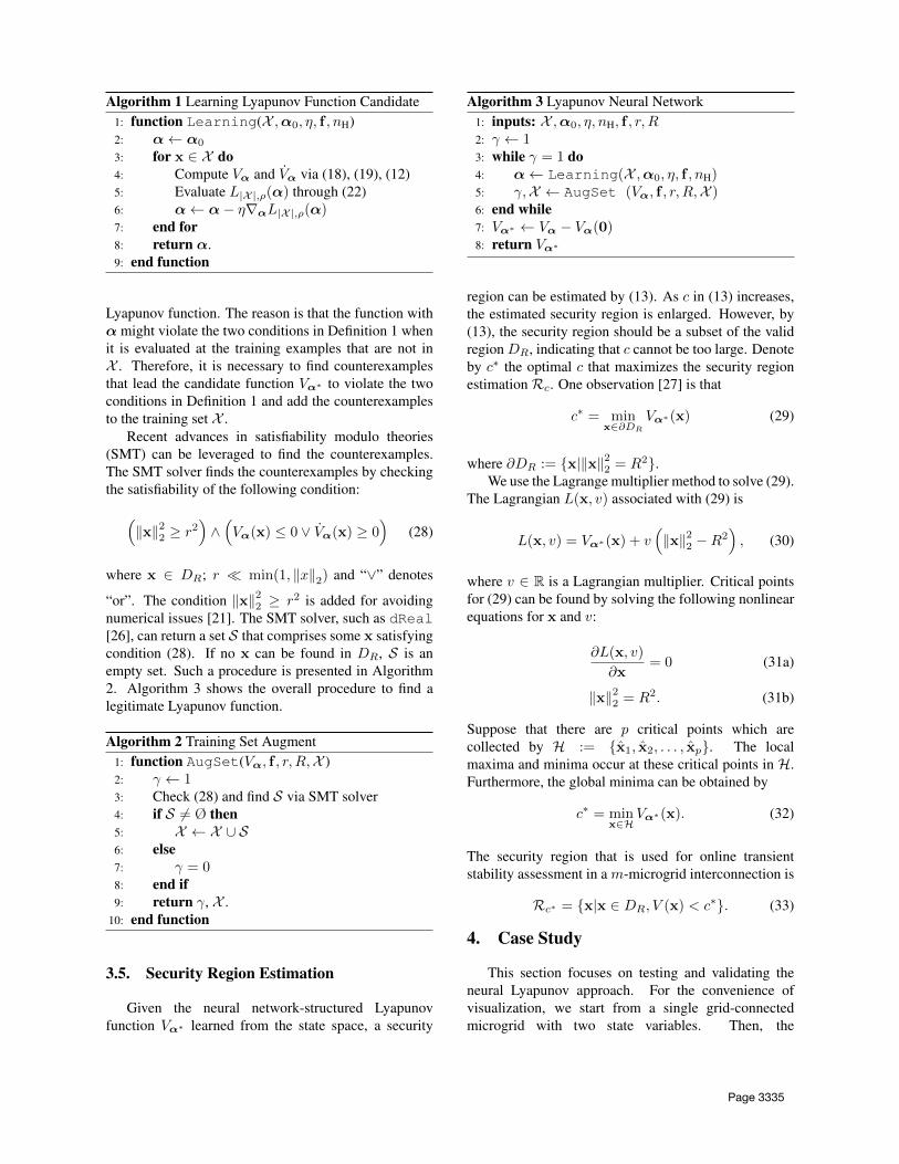
In this subsection, the neural Lyapunov approachis tested and validated in a grid-connected microgrid(Figure 1). A microgrid with PCC 1 is connected to therest of the grid via a distribution line whose impedanceis 1.20 + j1.10 p.u. The pre-dispatched setpoints formicrogrid 1 are P ∗1 = 0.3 p.u., Q∗1 = −0.16 p.u.,E∗1 = 1.05 p.u., and δ∗1 = ∠30◦. The control parametersof microgrid 1 are TA1 = 1.2, DA1 = 0.2, TV1 = 12,DV1 = 0.2. The terminal behavior of the rest of thegrid is modeled as a constant voltage source and itsterminal voltage is 1.00 p.u. The time-scale separationis not assumed, so we have two state variables δ′1 andE′1 which are the deviations of δ1 and E1 from theirequilibrium points. Note that the transient stability ofsuch a system cannot be assessed by the LMI-basedframework in [2], as it requires a special form ofdynamics.

Figure 1. A grid-connected microgrid

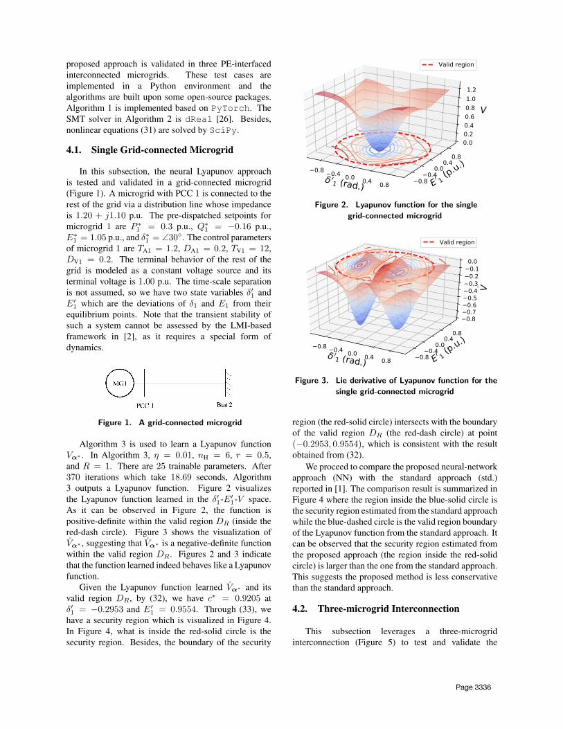
Algorithm 3 is used to learn a Lyapunov functionVα∗ . In Algorithm 3, η = 0.01, nH = 6, r = 0.5,and R = 1. There are 25 trainable parameters. After370 iterations which take 18.69 seconds, Algorithm3 outputs a Lyapunov function. Figure 2 visualizesthe Lyapunov function learned in the δ′1-E′1-V space.As it can be observed in Figure 2, the function ispositive-definite within the valid region DR (inside thered-dash circle). Figure 3 shows the visualization ofVα∗ , suggesting that Vα∗ is a negative-definite functionwithin the valid region DR. Figures 2 and 3 indicatethat the function learned indeed behaves like a Lyapunovfunction.

Given the Lyapunov function learned Vα∗ and itsvalid region DR, by (32), we have c∗ = 0.9205 atδ′1 = −0.2953 and E′1 = 0.9554. Through (33), wehave a security region which is visualized in Figure 4.In Figure 4, what is inside the red-solid circle is thesecurity region. Besides, the boundary of the security

Figure 2. Lyapunov function for the single

grid-connected microgrid

Figure 3. Lie derivative of Lyapunov function for the

single grid-connected microgrid

region (the red-solid circle) intersects with the boundaryof the valid region DR (the red-dash circle) at point(−0.2953, 0.9554), which is consistent with the resultobtained from (32).

We proceed to compare the proposed neural-networkapproach (NN) with the standard approach (std.)reported in [1]. The comparison result is summarized inFigure 4 where the region inside the blue-solid circle isthe security region estimated from the standard approachwhile the blue-dashed circle is the valid region boundaryof the Lyapunov function from the standard approach. Itcan be observed that the security region estimated fromthe proposed approach (the region inside the red-solidcircle) is larger than the one from the standard approach.This suggests the proposed method is less conservativethan the standard approach.

4.2. Three-microgrid Interconnection

This subsection leverages a three-microgridinterconnection (Figure 5) to test and validate the

Page 3336

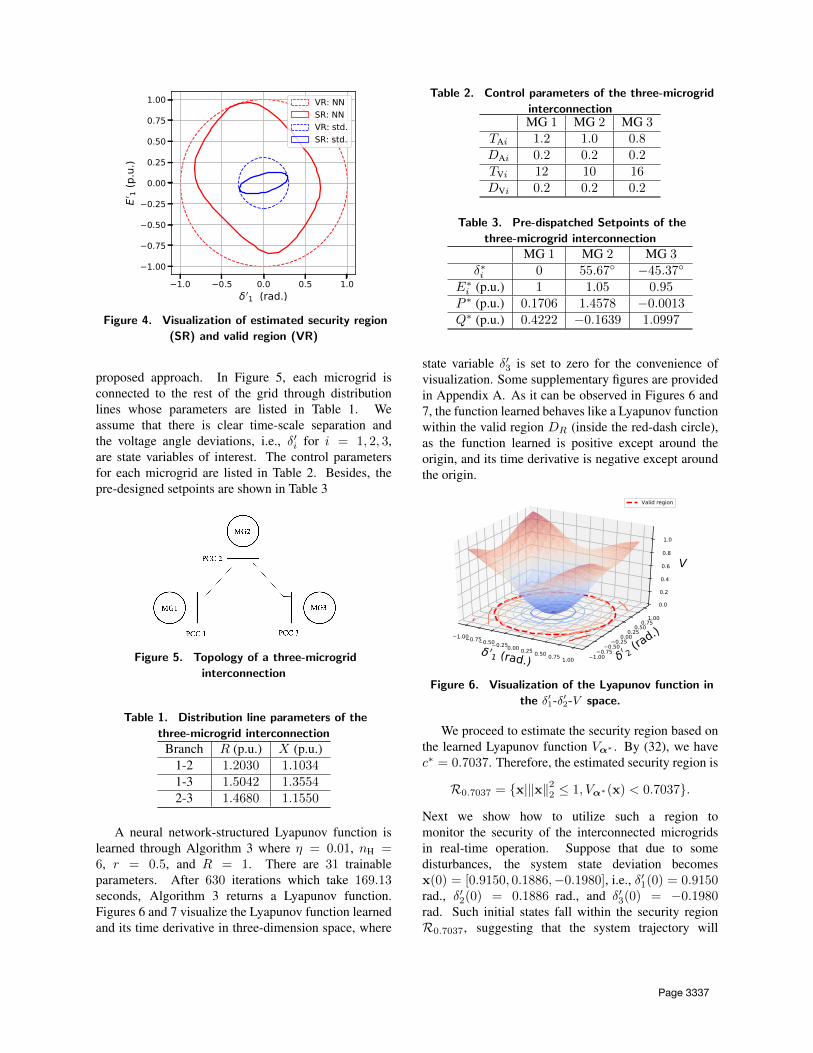
Figure 4. Visualization of estimated security region

(SR) and valid region (VR)

proposed approach. In Figure 5, each microgrid isconnected to the rest of the grid through distributionlines whose parameters are listed in Table 1. Weassume that there is clear time-scale separation andthe voltage angle deviations, i.e., δ′i for i = 1, 2, 3,are state variables of interest. The control parametersfor each microgrid are listed in Table 2. Besides, thepre-designed setpoints are shown in Table 3

Figure 5. Topology of a three-microgrid

interconnection

Table 1. Distribution line parameters of the

three-microgrid interconnection

Branch R (p.u.) X (p.u.)1-2 1.2030 1.10341-3 1.5042 1.35542-3 1.4680 1.1550

A neural network-structured Lyapunov function islearned through Algorithm 3 where η = 0.01, nH =6, r = 0.5, and R = 1. There are 31 trainableparameters. After 630 iterations which take 169.13seconds, Algorithm 3 returns a Lyapunov function.Figures 6 and 7 visualize the Lyapunov function learnedand its time derivative in three-dimension space, where

Table 2. Control parameters of the three-microgrid

interconnectionMG 1 MG 2 MG 3

TAi 1.2 1.0 0.8DAi 0.2 0.2 0.2TVi 12 10 16DVi 0.2 0.2 0.2

Table 3. Pre-dispatched Setpoints of the

three-microgrid interconnection

MG 1 MG 2 MG 3δ∗i 0 55.67◦ −45.37◦

E∗i (p.u.) 1 1.05 0.95P ∗ (p.u.) 0.1706 1.4578 −0.0013Q∗ (p.u.) 0.4222 −0.1639 1.0997

state variable δ′3 is set to zero for the convenience ofvisualization. Some supplementary figures are providedin Appendix A. As it can be observed in Figures 6 and7, the function learned behaves like a Lyapunov functionwithin the valid region DR (inside the red-dash circle),as the function learned is positive except around theorigin, and its time derivative is negative except aroundthe origin.

Figure 6. Visualization of the Lyapunov function in

the δ′1-δ′2-V space.

We proceed to estimate the security region based onthe learned Lyapunov function Vα∗ . By (32), we havec∗ = 0.7037. Therefore, the estimated security region is

R0.7037 = {x|‖x‖22 ≤ 1, Vα∗(x) < 0.7037}.

Next we show how to utilize such a region tomonitor the security of the interconnected microgridsin real-time operation. Suppose that due to somedisturbances, the system state deviation becomesx(0) = [0.9150, 0.1886,−0.1980], i.e., δ′1(0) = 0.9150rad., δ′2(0) = 0.1886 rad., and δ′3(0) = −0.1980rad. Such initial states fall within the security regionR0.7037, suggesting that the system trajectory will

Page 3337

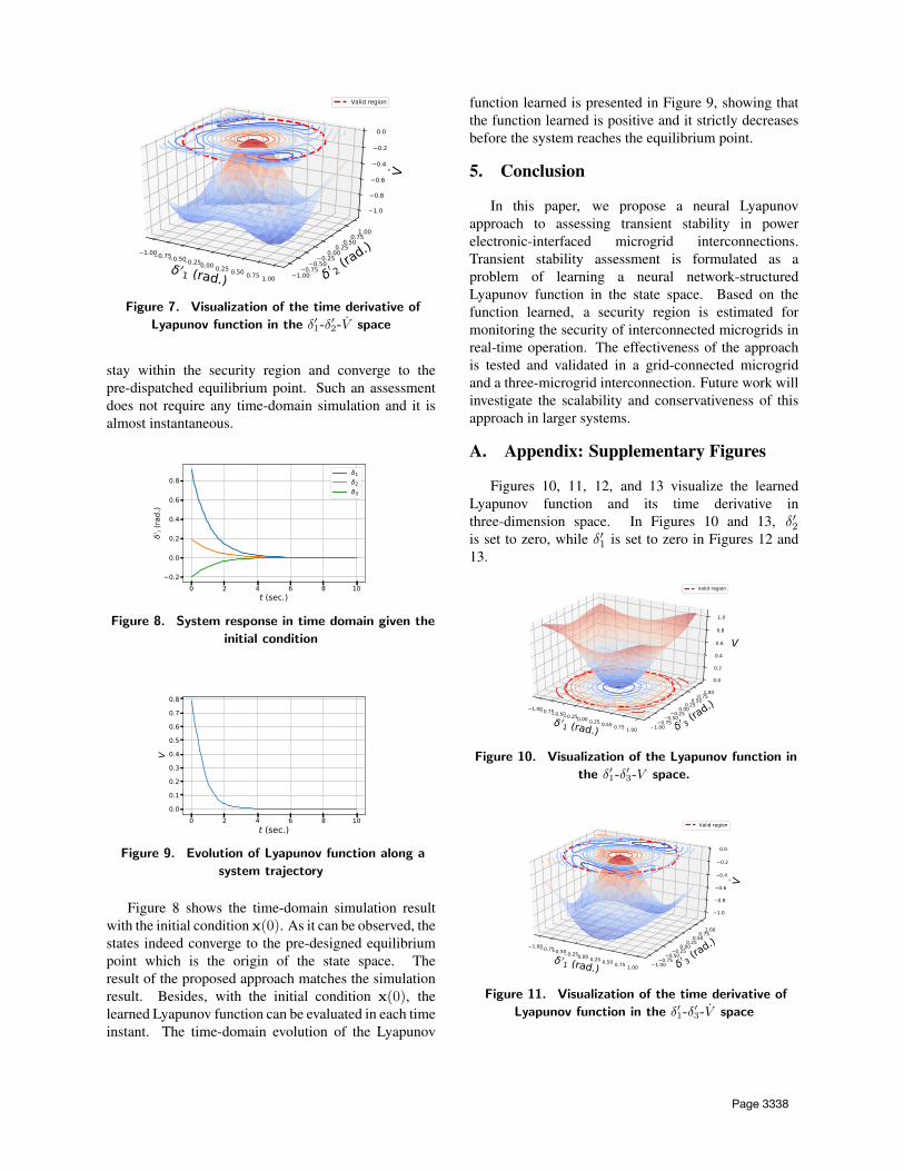
Figure 7. Visualization of the time derivative of

Lyapunov function in the δ′1-δ′2-V space

stay within the security region and converge to thepre-dispatched equilibrium point. Such an assessmentdoes not require any time-domain simulation and it isalmost instantaneous.

0 2 4 6 8 10t (sec.)

0.2

0.0

0.2

0.4

0.6

0.8

′ i (ra

d.)

123

Figure 8. System response in time domain given the

initial condition

0 2 4 6 8 10t (sec.)

0.00.10.20.30.40.50.60.70.8

V

Figure 9. Evolution of Lyapunov function along a

system trajectory

Figure 8 shows the time-domain simulation resultwith the initial condition x(0). As it can be observed, thestates indeed converge to the pre-designed equilibriumpoint which is the origin of the state space. Theresult of the proposed approach matches the simulationresult. Besides, with the initial condition x(0), thelearned Lyapunov function can be evaluated in each timeinstant. The time-domain evolution of the Lyapunov

function learned is presented in Figure 9, showing thatthe function learned is positive and it strictly decreasesbefore the system reaches the equilibrium point.

5. Conclusion

In this paper, we propose a neural Lyapunovapproach to assessing transient stability in powerelectronic-interfaced microgrid interconnections.Transient stability assessment is formulated as aproblem of learning a neural network-structuredLyapunov function in the state space. Based on thefunction learned, a security region is estimated formonitoring the security of interconnected microgrids inreal-time operation. The effectiveness of the approachis tested and validated in a grid-connected microgridand a three-microgrid interconnection. Future work willinvestigate the scalability and conservativeness of thisapproach in larger systems.

A. Appendix: Supplementary Figures

Figures 10, 11, 12, and 13 visualize the learnedLyapunov function and its time derivative inthree-dimension space. In Figures 10 and 13, δ′2is set to zero, while δ′1 is set to zero in Figures 12 and13.

Figure 10. Visualization of the Lyapunov function in

the δ′1-δ′3-V space.

Figure 11. Visualization of the time derivative of

Lyapunov function in the δ′1-δ′3-V space

Page 3338

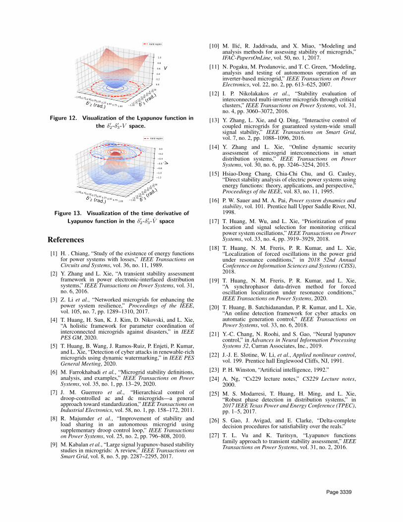
Figure 12. Visualization of the Lyapunov function in

the δ′2-δ′3-V space.

Figure 13. Visualization of the time derivative of

Lyapunov function in the δ′2-δ′3-V space

References

[1] H. . Chiang, “Study of the existence of energy functionsfor power systems with losses,” IEEE Transactions onCircuits and Systems, vol. 36, no. 11, 1989.

[2] Y. Zhang and L. Xie, “A transient stability assessmentframework in power electronic-interfaced distributionsystems,” IEEE Transactions on Power Systems, vol. 31,no. 6, 2016.

[3] Z. Li et al., “Networked microgrids for enhancing thepower system resilience,” Proceedings of the IEEE,vol. 105, no. 7, pp. 1289–1310, 2017.

[4] T. Huang, H. Sun, K. J. Kim, D. Nikovski, and L. Xie,“A holistic framework for parameter coordination ofinterconnected microgrids against disasters,” in IEEEPES GM, 2020.

[5] T. Huang, B. Wang, J. Ramos-Ruiz, P. Enjeti, P. Kumar,and L. Xie, “Detection of cyber attacks in renewable-richmicrogrids using dynamic watermarking,” in IEEE PESGeneral Meeting, 2020.

[6] M. Farrokhabadi et al., “Microgrid stability definitions,analysis, and examples,” IEEE Transactions on PowerSystems, vol. 35, no. 1, pp. 13–29, 2020.

[7] J. M. Guerrero et al., “Hierarchical control ofdroop-controlled ac and dc microgrids—a generalapproach toward standardization,” IEEE Transactions onIndustrial Electronics, vol. 58, no. 1, pp. 158–172, 2011.

[8] R. Majumder et al., “Improvement of stability andload sharing in an autonomous microgrid usingsupplementary droop control loop,” IEEE Transactionson Power Systems, vol. 25, no. 2, pp. 796–808, 2010.

[9] M. Kabalan et al., “Large signal lyapunov-based stabilitystudies in microgrids: A review,” IEEE Transactions onSmart Grid, vol. 8, no. 5, pp. 2287–2295, 2017.

[10] M. Ilic, R. Jaddivada, and X. Miao, “Modeling andanalysis methods for assessing stability of microgrids,”IFAC-PapersOnLine, vol. 50, no. 1, 2017.

[11] N. Pogaku, M. Prodanovic, and T. C. Green, “Modeling,analysis and testing of autonomous operation of aninverter-based microgrid,” IEEE Transactions on PowerElectronics, vol. 22, no. 2, pp. 613–625, 2007.

[12] I. P. Nikolakakos et al., “Stability evaluation ofinterconnected multi-inverter microgrids through criticalclusters,” IEEE Transactions on Power Systems, vol. 31,no. 4, pp. 3060–3072, 2016.

[13] Y. Zhang, L. Xie, and Q. Ding, “Interactive control ofcoupled microgrids for guaranteed system-wide smallsignal stability,” IEEE Transactions on Smart Grid,vol. 7, no. 2, pp. 1088–1096, 2016.

[14] Y. Zhang and L. Xie, “Online dynamic securityassessment of microgrid interconnections in smartdistribution systems,” IEEE Transactions on PowerSystems, vol. 30, no. 6, pp. 3246–3254, 2015.

[15] Hsiao-Dong Chang, Chia-Chi Chu, and G. Cauley,“Direct stability analysis of electric power systems usingenergy functions: theory, applications, and perspective,”Proceedings of the IEEE, vol. 83, no. 11, 1995.

[16] P. W. Sauer and M. A. Pai, Power system dynamics andstability, vol. 101. Prentice hall Upper Saddle River, NJ,1998.

[17] T. Huang, M. Wu, and L. Xie, “Prioritization of pmulocation and signal selection for monitoring criticalpower system oscillations,” IEEE Transactions on PowerSystems, vol. 33, no. 4, pp. 3919–3929, 2018.

[18] T. Huang, N. M. Freris, P. R. Kumar, and L. Xie,“Localization of forced oscillations in the power gridunder resonance conditions,” in 2018 52nd AnnualConference on Information Sciences and Systems (CISS),2018.

[19] T. Huang, N. M. Freris, P. R. Kumar, and L. Xie,“A synchrophasor data-driven method for forcedoscillation localization under resonance conditions,”IEEE Transactions on Power Systems, 2020.

[20] T. Huang, B. Satchidanandan, P. R. Kumar, and L. Xie,“An online detection framework for cyber attacks onautomatic generation control,” IEEE Transactions onPower Systems, vol. 33, no. 6, 2018.

[21] Y.-C. Chang, N. Roohi, and S. Gao, “Neural lyapunovcontrol,” in Advances in Neural Information ProcessingSystems 32, Curran Associates, Inc., 2019.

[22] J.-J. E. Slotine, W. Li, et al., Applied nonlinear control,vol. 199. Prentice hall Englewood Cliffs, NJ, 1991.

[23] P. H. Winston, “Artificial intelligence, 1992.”

[24] A. Ng, “Cs229 lecture notes,” CS229 Lecture notes,2000.

[25] M. S. Modarresi, T. Huang, H. Ming, and L. Xie,“Robust phase detection in distribution systems,” in2017 IEEE Texas Power and Energy Conference (TPEC),pp. 1–5, 2017.

[26] S. Gao, J. Avigad, and E. Clarke, “Delta-completedecision procedures for satisfiability over the reals.”

[27] T. L. Vu and K. Turitsyn, “Lyapunov functionsfamily approach to transient stability assessment,” IEEETransactions on Power Systems, vol. 31, no. 2, 2016.

Page 3339