A Mathematical Introduction to Conformal Field Theory(LNP NS m43 - Schottenloher
Dec 02, 2014
Welcome message from author
This document is posted to help you gain knowledge. Please leave a comment to let me know what you think about it! Share it to your friends and learn new things together.
Transcript
Lecture Notes in Physics New Series m: Monographs
Editorial Board
H. Araki, Kyoto, Japan E. Br~zin, Paris, France J. Ehlers, Potsdam, Germany U. Frisch, Nice, France K. Hepp, Zfirich, Switzerland R. L. Jaffe, Cambridge, MA, USA R. Kippenhahn, G6ttingen, Germany H. A. Weidenmfiller, Heidelberg, Germany J. Wess, Mfinchen, Germany J. Zittartz, KSln, Germany
Managing Editor
W. Beiglb/Sck Assisted by Mrs. Sabine Lehr c/o Springer-Verlag, Physics Editorial Department II Tiergartenstrasse 17, D-69121 Heidelberg, Germany
The Editorial Policy for Monographs
The series Lecture Notes in Physics reports new developments in physical research and teaching- quickly, informally, and at a high level. The type of material considered for publication in the New Series m includes monographs presenting original research or new angles in a classical field. The timeliness of a manuscript is more important than its form, which may be preliminary or tentative. Manuscripts should be reasonably self-contained. They will often present not only results of the author(s) but also related work by other people and will provide sufficient motivation, examples, and applications. The manuscripts or a detailed description thereof should be submitted either to one of the series editors or to the managing editor. The proposal is then carefully refereed. A final decision concerning publication can often only be made on the basis of the complete manuscript, but otherwise the editors will try to make a preliminary decision as definite as they can on the basis of the available information. Manuscripts should be no less than loo and preferably no more than 400 pages in length. Final manuscripts should preferably be in English, or possibly in French or German. They should include a table of contents and an informative introduction accessible also to readers not particularly familiar with the topic treated.Authors are free to use the material in other publications. However, if extensive use is made elsewhere, the publisher should be informed. Authors receive jointly 50 complimentary copies of their book. They are entitled to purchase further copies of their book at a reduced rate. As a rule no reprints of individual contributions can be supplied. No royalty is paid on Lecture Notes in Physics volumes. Commitment to publish is made by letter of interest rather than by signing a formal contract. Springer-Verlag secures the copyright for each volume.
The Production Process
The books are hardbound, and quality paper appropriate to the needs of the author(s) is used. Publication time is about ten weeks. More than twenty years of experience guarantee authors the best possible service. To reach the goal of rapid publication at a low price the technique of photographic reproduction from a camera-ready manuscript was chosen. This process shifts the main responsibility for the technical quality considerably from the publisher to the author. We therefore urge all authors to observe very carefully our guidelines for the preparation of camera-ready manuscripts, which we will supply on request. This applies especially to the quality of figures and halftones submitted for publication. Figures should be submitted as originals or glossy prints, as very often Xerox copies are not suitable for reproduction. For the same reason, any writing within figures should not be smaller than 2.5 mm. It might be useful to look at some of the volumes already published or, especially if some atypical text is planned, to write to the Physics Editorial Department of Springer-Verlag direct. This avoids mistakes and time-consum- ing correspondence during the production period. As a special service, we offer free of charge LATEX and TEX macro packages to format the text according to Springer-Verlag's quality requirements. We strongly recommend au- thors to make use of this offer, as the result will be a book of considerably improved technical quality. Manuscripts not meeting the technical standard of the series will have to be returned for improvement. For further information please contact Springer-Verlag, Physics Editorial Department II, Tiergartenstrasse 17, D-69121 Heidelberg, Germany.
Martin Schottenloher
A Mathematical Introduction to Conformal Field Theory
Based on a Series of Lectures given at the Mathematisches Institut der Universit~it Hamburg
Springer
Author
Martin Schottenloher Mathematisches Institut, LMU Mtinchen Theresienstrasse 39 D-80333 Mtinchen, Germany
cIP data applied for.
Die Deutsche B i b l i o t h e k - C I P - E i n h e i t s a u f n a h m e
Schottenioher, Martin: A mathemat i ca l i n t roduc t ion to eonformal field theory : lectures at the Ma thema t i s ches Ins t i tu t der Universitfi t H a m b u r g / M a r t i n S c h o t t e n l o h e r . - Berl in ; H e i d e l b e r g ; New York ; Barcelona ; Budapest ; Hong Kong ; London ; Mi lan ; Paris ; Santa C l a r a ; Singapore ; Tokyo : Springer, 1997
(Lecture notes in physics : N.s. M, Monographs ; 43) Einheitssacht.: Eine mathematische Einfiihrung in die konforme Feldtheorie <engl. > ISBN 3-540-61753-1
NE: Lecture notes in physics / M
ISSN o94o-7677 (Lecture Notes in Physics. New Series m: Monographs) ISBN 3-54o-61753-1 Springer-Verlag Berlin Heidelberg New York
This work is subject to copyright. All rights are reserved, whether the whole or part of the material is concerned, specifically the rights of translation, reprinting, re-use of illustrations, recitation, broadcasting, reproduction on microfilms or in any other way, and storage in data banks. Duplication of this publication or parts thereof is permitted only under the provisions of the German Copyright Law of September 9, 1965, in its current version, and permission for use must always be obtained from Springer-Verlag. Violations are liable for prosecution under the German Copyright Law.
© Springer-Verlag Berlin Heidelberg 1997 Printed in Germany
The use of general descriptive names, registered names, trademarks, etc. in this publica- tion does not imply, even in the absence of a specific statement, that such names are exempt from the relevant protective laws and regulations and therefore free for general use.
Typesetting: Camera-ready by author Cover design: design ~r production GmbH, Heidelberg SPIN: 105418o4 5513144-54321o - Printed on acid-free paper
Preface
The present notes consist of two parts of approximately equal length. The first part gives an elementary, detailed and self-contained math- ematical exposition of classical conformal symmetry in n dimen- sions and its quantization in two dimensions. Central extensions of Lie groups and Lie algebras are studied in order to explain the appearance of the Virasoro algebra in the quantization of two- dimensional conformal symmetry. The second part surveys some topics related to conformal field theory: the representation theory of the Virasoro algebra, some aspects of conformal symmetry in
string theory, a set of axioms for a two-dimensional conformally invariant quantum field theory and a mathematical interpretation of the Verlinde formula in the context of semi-stable vector bundles on a Riemann surface. In contrast to the first part only few proofs are provided in this less elementary second part of the notes.
These notes constitute - except for corrections and supplements - a translation of the prepublication "Eine mathematische Einfiih- rung in die konforme Feldtheorie" in the preprint series Hamburger Beitr~ge zur Mathematik, Volume 38 (1995). The notes are based on a series of lectures I gave during November/December of 1994 while holding a Gastdozentur at the Mathematisches Seminar der Universitiit Hamburg and on similar lectures I gave at the Universitd de Nice during March/April 1995.
It is a pleasure to thank H. Brunke, R. Dick, A. Jochens and P. Slodowy for various helpful comments and suggestions for correc- tions. Moreover, I want to thank A. Jochens for writing a first version of these notes and for carefully preparing the 1.4TEX file of an expanded English version. Finally, I would like to thank the Springer production team for their support.
Munich, January 1997 Martin Schottenloher
v I
Key words and phrases:
conformal field theory, conformal transformation, conformal group, central extensions of groups and of Lie algebras, Virasoro algebra and its representations, string theory, Osterwalder-Schrader ax- ioms, primary fields, fusion rules, Verlinde formula, moduli space of parabolic bundles on a Riemann surface.
Mathematics Subject Classification (1991)"
Primary: 81 T 05, 81 T 40, 81 R 10 Secondary: 14 H 60, 17 B 68
E-mail" [email protected] (Martin Schottenloher) [email protected] (Andreas Jochens)

Contents
Introduct ion 1
I Mathemat ica l Prel iminaries 3
1 Conformal Transformations and Conformal Killing Fields 3 1.1 Semi-Riemannian Manifolds . . . . . . . . . . . . . 3
1.2 Conformal Transformations . . . . . . . . . . . . . 5
1.3 Conformal Killing Fields . . . . . . . . . . . . . . . 9
1.4 Classification of Conformal Transformations . . . . 12
1.4.1 Case 1 : n - p + q > 2 . . . . . . . . . . . . 12
1.4.2 Case 2: Euclidean Plane (p = 2, q = 0) . . . 16
1.4.3 Case 3: Minkowski Plane (p = q = 1) . . . . 18
2 T h e C o n f o r m a l G r o u p 20
2.1 Conformal Compactif ication of R p,q . . . . . . . . . 20
2.2 The Conformal Group of R p'q for p + q > 2 . . . . . 24
2.3 The Conformal Group of R 2'° . . . . . . . . . . . . 28
2.4 The Conformal Group of R 1'1 . . . . . . . . . . . . 32
3 Central Extensions of G r o u p s 36 3.1 Central Extensions . . . . . . . . . . . . . . . . . . 36
3.2 Quant iza t ion of Symmetries . . . . . . . . . . . . . 39
3.3 Equivalence of Central Extensions . . . . . . . . . . 44
4 Central Extensions of Lie Algebras and Bargmann's Theorem 47 4.1 Central Extensions and Equivalence . . . . . . . . . 47
4.2 Bargmann ' s Theorem . . . . . . . . . . . . . . . . . 51
5 The Virasoro Algebra 56 5.1 W i t t Algebra and Infinitesimal Conformal
Transformations of the Minkowski Plane . . . . . . 56
5.2 W i t t Algebra and Infinitesimal Conformal
Transformations of the Euclidean Plane . . . . . . . 58
VIII
5.3 The Virasoro Algebra as a Central Extension of the Witt Algebra . . . . . . . . . . . . . . . . . . 60
I I F i r s t S t e p s T o w a r d s C o n f o r m a l F i e l d T h e o r y 65
6 R e p r e s e n t a t i o n T h e o r y of the Virasoro Algebra 65 6.1 Unitary and Highest-Weight Representations . . . . 65 6.2 Verma Modules . . . . . . . . . . . . . . . . . . . . 66 6.3 The Kac Determinant . . . . . . . . . . . . . . . . 69 6.4 Indecomposability and Irreducibility
of Representations . . . . . . . . . . . . . . . . . . 74
7 P ro j ec t i ve Rep re sen t a t i ons of Diff+ (S) and M o r e 76
8 S t r ing T h e o r y as a Conformal Field T h e o r y 78 8.1 Action Functionals and Equations of Motion
for Strings . . . . . . . . . . . . . . . . . . . . . . . 78 8.2 Quantization . . . . . . . . . . . . . . . . . . . . . 87
9 Founda t ions of Two-Dimens iona l Confo rmal Q u a n t u m Field T h e o r y 95 9.1 Axioms for Two-Dimensional Euclidean
Quantum Field Theory . . . . . . . . . . . . . . . . 95 9.2 Conformal Fields and the Energy-Momentum Tensor 101 9.3 Primary Fields, Operator Product Expansion
and Fusion . . . . . . . . . . . . . . . . . . . . . . . 104 9.4 Other Approaches to Axiomatization . . . . . . . . 108
10 M a t h e m a t i c a l Aspec t s of the Verl inde Fo rmula 110 10.1 The Moduli Space of Representations
and Theta Functions . . . . . . . . . . . . . . . . . 110 10.2 The Verlinde Formula . . . . . . . . . . . . . . . . . 118 10.3 Fusion Rules for Surfaces with Marked Points . . . 121 10.4 Combinatorics on Fusion Rings . . . . . . . . . . . 129
R e f e r e n c e s 1 3 2
I n d e x 1 3 8
Introduct ion
Conformal field theory in two dimensions has its roots in statis- tical physics (cf. [BPZ84] as a fundamental work and [Gin89] for an introduction) and it has close connections to string theory and other two-dimensional field theories in physics (cf. e.g. [LPSA94]). In particular, all massless field theories are conformally invariant. The special feature of conformal field theory in two dimensions is the existence of an infinite number of independent symmetries of the system, leading to corresponding constraints. These symme- tries can be understood as infinitesimal conformal symmetries of the Euclidean plane or, more generally, of surfaces with a confor- mal structure, i.e. Riemann surfaces. Since the conformal and
orientation-preserving transformations on open subsets of the Eu- clidean plane are holomorphic functions, there is a close connection between conformal field theory and function theory. This connec- tion yields remarkable results on moduli spaces of vector bundles over compact Riemann surfaces, and therefore provides an interest- ing example of how physics can be applied to mathematics.
The original purpose of the lectures on which the present text is based was to describe and to explain the role the Virasoro algebra plays in the quantization of conformal symmetries in two dimen- sions. In view of the usual difficulties of a mathematician reading research articles or monographs on conformal field theory, it was an essential concern of the lectures not to rely on background know- ledge of standard methods in physics. Instead, the aim was to try to present all the necessary concepts and methods on a purely mathematical basis. This explains the adjective "mathematical" in the title. Another essential motivation for the lectures was to discuss the confusing use of language by physicists, who for exam- ple emphasize that the conformal group of all holomorphic maps of the complex plane is infinite dimensional- which is not true. What physicists really seem to mean by this statement is that a certain Lie algebra closely related to conformal symmetry, namely the Witt algebra or its central extension, the Virasoro algebra, is infinite dimensional.
Clearly, with these objectives the lectures could hardly cover an es- sential part of actual conformal field theory. Indeed, in the course of
2 Introduction
the present text, conformal field theory does not appear before Sect. 6, which treats the representation theory of the Virasoro algebra as a first topic of conformal field theory. This text should therefore be seen as a preparation for conformal field theory or as an intro- duction to conformal field theory for mathematicians focussing on some background material in geometry and algebra. Physicists may find the detailed discussion of some elementary structures useful.
In view of the above-mentioned tasks, it makes sense to start with a detailed description of the conformal transformations in arbitrary dimensions and for arbitrary signatures (Sect. 1) and to deter- mine the associated conformal groups (Sect. 2). In particular, the conformal group of the Minkowski plane is infinite dimensional, while the conformal group of the Euclidean plane is finite dimen- sional. The next two sections are concerned with central extensions of groups and Lie algebras and their classification by cohomology. Central extensions are needed, because the symmetry group of a quantized system usually is a central extension of the classical sym- metry group. Section 5 leads to the Virasoro algebra as the unique non-trivial central extension of the Witt algebra. The Witt algebra is the essential component of the classical infinitesimal conformal symmetry in two dimensions for the Euclidean plane as well as for the Minkowski plane.
This concludes the first part of the text, which is detailed and comparatively elementary and which provides essentially all proofs. These characterizations are no longer true for the second part, which starts with the representation theory of the Virasoro alge- bra and also contains the Kac formula (Sect. 6). It then shortly deals with the representation theory of Diff+(S) (Sect. 7) and it explains the conformal symmetry in string theory (Sect. 8) with an application to the representation theory of the Virasoro alge- bra. The last two sections report on a system of axioms for two- dimensional conformally invariant quantum field theories (Sect. 9) and on the Verlinde formula as an application of conformal field theory to mathematics (Sect. 10).
Part I
M a t h e m a t i c a l Prel iminaries
Conformal Transformations and Conformal Killing Fields
1.1 S e m i - R i e m a n n i a n Manifolds
Def ini t ion 1.1 A semi-Riemannian manifold is a pair (M, g) con- sisting of a differentiable (i.e. C °~) manifold M and a differentiable tensor field g which assigns to each point a E M a non-degenerate and symmetric bilinear form on the tangent space TaM:
ga " TaM x TaM ~ R.
In local coordinates x l , . . . , x ~ of the manifold M (given by a chart ¢" U ~ V on an open subset U in M, ¢(a) = (xl(a) , . . . ,xn(a)), a E M) the bilinear form g~ on TaM can be written as
ga (X, Y) = g~v (a) X ~ Y v.
Here, the tangent vectors X = X~'i)~,, Y = Y~'O~, E TaM are de- scribed with respect to the basis
0 ~'= ~=1 n
of the tangent space TaM. By assumption, the matrix
is non-degenerate and symmetric for all a E U, i.e. one has
det (g~v(a)) ~ 0 and (g~v(a))T= (g~,v(a)).
Moreover, the differentiability of g implies that the coefficients g~,v(a) of the matrix (g~,~,(a)) depend differentiably on a. In gen- eral, however, the condition g~,v(a)X~'X V > 0 does not hold for all Z # 0, i.e. the matrix (g~,~,(a)) is not required to be positive definite. This property distinguishes Riemannian manifolds from general semi-Riemannian manifolds.
1. Conformal Transformations and Conformal Killing Fields
Examples"
• R p'q --" ( R p+q, gP'q) for p, q E N where
p p+q
( x , v ) . = - i=1 i=p+l
Hence
X i y i.
( g ' ~ ) = ( l P 0 / = d i a g ( l " " ' l ' - l " ' " - l ) ' 0 - l q
* R 1'3 or ]~3,1. the usual Minkowski space.
• R 1'1" the two-dimensional Minkowski space (the Minkowski plane).
• R2'°: the Euclidean plane.
• S 2 C R3'°: Compactification of R2'°; the structure of a Rie- mannian manifold on the 2-sphere S 2 is induced by the inclu- sion in R 3'°.
• S x S c I~2'2: Compactification of R 1'1. More precisely: S x S c R 2'° xR °'2 ~ R 2'2 where the first circle S = S 1 is contained in R 2,°, the second one in R °'2 and where the structure of a semi-Riemannian manifold on S x S is induced by the inclusion in R 2,2.
• Similarly, S p x Sq C R p+l'° X R 0'q+l __e'° ]~p-t-l,q+l, with the
p-sphere ~ = {Z e RP+I"g~'+I'°(X,X)= 1} C R p+l'° and
the q-sphere S q C R °'q+l, as a generalization of the previous example, yields a compactification of R p'q for p, q >_ 1. This compact semi-Riemannian manifold will be denoted by S p'q for all p, q >_ 0.
In the following, we will use the above examples of semi-Riemannian manifolds and their open subspaces o n l y - except for the quadrics N p'q occurring in (2.1). (These quadrics are locally isomorphic to S p,q from the point of view of conformal geometry.)
1.2 Conformal Transformations 5
1.2 C o n f o r m a l T r a n s f o r m a t i o n s
Def in i t ion 1.2 Let (M, g) and (M', g') be two semi-Riemannian manifolds and let U C M, V C M ~ be open subsets of M and M' respectively. A differentiable map ~ : U ~ V is a conformal trans- formation, or simply conformal, if there is a differentiable function ~" U --o R+ such that ~*g~ = ~2g, where
~* g' (X, Y ) " = g' (T~(X) , T ~ ( Y ) )
and T~ : TU ~ T V denotes the tangent map (derivative) of ~. is called the conformal factor of ~. Sometimes a conformal
transformation ~ : U ~ V is additionally required to be bijective and/or orientation preserving.
In local coordinates of M and M'
* ' = ' o.vo . (~ g ).~ (a) gij (~ (a)) i '
Hence, ~ is conformal if and only if
(1)
in the coordinate neighborhood of each point.
Note that for a conformal transformation ~ the tangent maps T ~ : TaM --* T~,(a)M ~ are bijective for each point a E U. Hence, by the inverse mapping theorem a conformal transformation is always locally invertible as a differentiable map.
Examples:
Local isometries, i.e. differentiable mappings ~ with ~ '9 ~ - 9, are conformal transformations with conformal factor Ft = 1.
• In order to study conformal transformations on the Euclidean plane R 2'° we identify R 2,° ~ C and write z = x + iy for z E C
with "real coordinates" (x, y) E R. Then a differentiable map : M ~ C on a connected open subset M C C is conformal
according to (1) with conformal factor ~ : M - . R+ if and only if for u = Re ~ and v = Im
1. Conformal Transformations and Conformal Killing Fields
u~2 + v~2 = f~2 = uy2 + vy ~ ~ 0 , u~uy + v~vy = O. (2)
These equations are, of course, satisfied by the holomorphic (resp. anti-holomorphic) functions from M to C because of the Cauchy-Riemann equations ux = vy, u~ = -vx (resp.
2 2 u~ = -vy, uy = v~) if u~ + v~ ~ 0. For holomorphic or anti- 2 +v~ ~ 0 is equivalent to det D~ =fi 0 holomorphic functions, u~
where D~ denotes the Jacobi matrix representing the tangent map T~ of ~.
Conversely, for a general conformal transformation ~o the equa- tions (2) imply that (u~, v~) and (u~, v~) are perpendicular vectors in R 2'° of equal length ~ ~ 0. Hence, (u~, v~) =
(-vy, uy) or (u~, v~) = (vy,-uy), i.e. ~ is holomorphic or anti-holomorphic.
As a first i m p o r t a n t resul t , we have shown that the con- formal transformations ~ : M ~ C with respect to the Eu- clidean structure on M C C are the locally invertible holo- morphic or anti-holomorphic functions. The conformal factor of ~ is I det D~o I.
• With the same identification R 2,° =~ C a linear map ~ : R 2,° ---. R 2'° with representing matrix
A = A ~ = ( ac db)
is conformal if and only if a 2 + c 2 -~ 0 and a = d, b = - c or a = - d , b = c. As a consequence, for ¢ = a + ic ~ O, ~ is of the form z ~ Cz or z ~ ¢5.
These conformal and linear transformations are angle pre- serving in the following sense: for points z, w E C \ {0} the number w(z, w)"= Wbi ~ determines the (Euclidean) angle be-
tween z and w up to orientation. In the case of ~o(z) = Cz it follows that
~z¢w =
and the same holds for ~(z) = ~ .
1.2 Conformal Transformations 7
Conversely, the linear maps ~a with w(~o(z), ~o(w)) = w(z, w) for all z, w E C \ {0} are conformal transformations. We conclude that a linear map ~o : IR 2'° --+ IR 2'° is a conformal transformation for the Euclidean plane if and only if it is angle preserving.
As a consequence, the conformal transformations ~o : M ---+ C can also be characterized as those mappings which pre-
serve the angles infinitesimally: let z(t), w(t) be differentiable curves in M with z(0) = w(0) = a and ~(0) # 0 # w(0), where ~(0) = d a~z(t)it=o is the derivative of z(t) at t = 0. Then w(}(0), ~b(0)) determines the angle between the curves z(t) and w(t) at the common point a. Let z~ = ~o o z and w~ -- ~o o w be the image curves. By definition, ~o is called to preserve angles infinitesimally if and only if w(~(0), w ( 0 ) ) = co(~(0), uJ~(0)) for all points a 6 M and all curves z(t), w(t) in M through a = z(0) = w(0) with ~(0) # 0 # ~b(0). Note that d~(0) = D~o(a)(~(0)) by the chain rule. Hence, by the above characterization of tbe linear conformal transforma- tions, ~o preserves angles infinitesimally if and only if D~o(a) is a linear conformal transformation for all a 6 M which by (2) is equivalent to ~o being a conformal transformation.
Again in the case of IR 2'° ~ C one can deduce from the above results that the conformal, orientation-preserving and bijec- tive transformations ]R 2'° --+ ]R 2'° are the entire holomorphic functions ~0 • C ~ C with holomorphic inverse functions ~0 -1 • C ~ C, i.e. the biholomorphic functions ~0" C --+ C. These functions are simply the complex-linear affine maps of the form
= Cz + r, z C,
with ~ , r 6 C , ~ # O.
The group of all conformal, orientation-preserving invertible transformations ]R 2'° ---+ ]R 2'° of the Euclidean plane can thus be identified with (C \ {0}) x C, where the group law is given
by (¢, = (¢¢', +
(This is an example of a semi-direct product of groups.) In
1. Con[ormal Transformations and Conformal Killing Fields
particular, this abelian group is a four-dimensional real mani- fold.
• The stereographic projection
7r " \ {(0, 0,1)} R ,o
is conformal wi th f~ = ~ In order to prove this it suffices ]-~.
to show tha t the inverse map ~o "= zr -1 • R 2'° ---. S 2 C R a'° is
a conformal t ransformat ion. We have
1 ~(~c, r/) = 1 + r 2 (2~, 2r/, r 2 - 1),
for (~, r/) e R 2 and r = V/~2+ 7/2.
X1 = ~ , X 2 = ~ we get
For the tangent vectors
d T~o(X1) : d] ~o(( + t, 71) 1t:o
= :2 1 + r 2 (r2 + 1 - 2 ( 2, - 2 ( r l , 2( )
T~o(X2) = 2 1 + r 2 ( - 2 ( ~ , r 2 + 1 - 27/2, 2r/).
Hence
(2)2 g' (T~o(Xi), T~o(X~)) = 1 + r 2 (Sij) ,
i.e. A = ~ 2 is the conformal factor of ~o. Thus, r =~o
the conformal factor fl = A -1 1(1 + r 2) = 1 = ~ l-z"
-I has
Similarly, the stereographic project ion of the n-sphere,
zr • S~ \ { ( 0 , . . . , 0 , 1)} ---~ I~ ~,°,
is a conformal map.
R2, 0 S X S C C x C -'~ R 2'0 × R 2'0 -'~ R 4'0,
( l+ia + l + i a - ) aft= l (x 4-y) 1- ia+ ~ 1 - i a - ~ : ~ 2
1.3 Conformal Killing Fields
is a conformal map into the Riemannian version of S x S.
Furthermore, ~o : R 2 -. S 1'1 = S x S can also be regarded as
a conformal map with respect to the metric on R 2 given by
the bilinear form
1 ((x, y), (x', y')) .= ~(xy' + yx').
This is a Minkowski metric on R 2, for which the coordinate
axis coincides with the light cone
L = { (x, y)" ((x, y), (x, y)> = 0}
in 0 E R ~. With this metric, R 2 is isometrically isomorphic to R 1'1 with respect to the isomorphism ¢:R 1'1 --. R 2,
(~, y) ~ (~ + y, • - y).
• ~" R 1,1 ~ S 1'1 = S x S "" R 2'° x R °,2
(x, y) ~ ~-~-~1, ~-+1, ¢-÷1, ¢-+1
is a conformal map into the non-Riemannian version g1,1 of S x S. Hence it, yields a conformal compactification of the Minkowski plane. ( corresponds to the composition ~o o ¢ up
to a permutation of coordinates.
• The composition of two conformal maps is conformal. One can treat the two preceding examples using this property.
• If ~ • M ~ M ~ is a bijective conformal transformation with conformal factor f~ then ~ is a diffeomorphism (i.e. ~o -1 is differentiable), and, moreover, qo -1 • M' ~ M is conformal
1 This property has been used in with conformal factor ~. the investigation of the above example on the stereographic
projection.
1.3 Conformal Killing Fields
In the following, we want to study the conformal maps ~ : M ---. M ~ between open subsets M, M ~ C R p'q, p + q = n > 1. To begin with, we will classify them by an infinitesimal argument:
10 1. ConformM Transformations and Conformal Killing Fields
Let X • M C ]R p'q --. R n be a differentiable vector field. Then
;y = x
for differentiable curves -y = -y(t) in M is an autonomous differential equation. The local one-parameter group (99 x) tea corresponding to X satisfies
d (~x (t, a)) = X (~x (t, a)) dt
with initial condition ~x (0, a) = a. Moreover, for every a E U, ~o x (., a ) i s the unique maximal solution of-~ = X (7) defined on the maximal interval ] t ; , t+[. Let Mt "= {a e M ' t 2 < t < t +} and ~o x ( a ) "= ~o x (t, a) for a E Mr. Then Mt C i is an open subset of M and ~ x . Mt ~ M-t is a diffeomorphism. Furthermore, we have ~x o ~X(a) = 9~x+t(a) if a e Mt+s N Ms and ~x (a) E Mr, and, of course, ~o x = idM, M0 = M. In particular, the local one-parameter group (~ox)t~ satisfies the flow equation
d = x .
Def in i t ion 1.3 A vector field X on M C R p'q is called a conformal Killing field if ~x is conformal for all t in a neighborhood of O.
T h e o r e m 1.4 Let M C lRp,q be open, g = f ' q and X a conformal Killing field with coordinates
X : (X 1,.. . ,x n) :XYOv
with respect to the canonical cartesian coordinates on R n. there is a differentiable function a" M --, R, so that
Then
X, , : + X~,, = ague.
Here we use the notation: f,~ "= O~f , X , "= gu~X ~.
P r o o f Let X be a conformal Killing field, (~t) the associated local one-parameter group and ~t" Mt ~ R +, such that
(~tg)uu (a) -- gij (~t (a))au~ ~ 0v~t" ---- (~t(a)) 2 g~u (a).
1.3 Conformal Killing Fields 11
By differentiation with respect to t at t - 0 we get (gij is constant!)"
__d (f~2(a) g~v (a))[t=o _ _d (gij (~t (a)) O~qa ti O.,¢d~ [ dt dt t=o
- o ' o ~ 4 + g,jO. 'o~i4 - g~j ~ a o qao -- gij O, Xi(a) ~ + gij 6~ O~X j (a)
= O,X~(a) + OvX~(a).
d f~2(a) it=o. Hence, the statement follows with ~;(a) = ~ I
If g,~ is not constant, we have
(Lxg),~ = X~,;~ + X~;, = ag,~.
Here, Lx is the Lie derivative and a semicolon in the index denotes the covariant derivative corresponding to the Levi-Civita connec- tion for g.
Def in i t ion 1.5 A differentiable function a : M C ~P'q ~ ~ i8 called a conformal Killing factor if there is a conformal Killing field X , such that
X.,~ + X~,. = ~g.~.
(Similarly, for general semi-Riemannian manifolds on coordinate neighborhoods:
X,;~ + X~;, = ag,~.)
T h e o r e m 1.6 ~ : M ~ R is a conformal Killing factor if and only if
(n - 2) ~,~ + g,~Ag~ = 0,
where Ag = gklOkOt is the Laplace-Beltrami operator for g = gP'q.
P r o o f "=~"" Let a • M ~ R a n d X , , ~ + X ~ , , = Rg,~ (M C Rp,q, g = gp, q). Then from
0k0t (X,,~) = 0~0k (X~,t) etc.
it follows that
= aka, (x~,~ + x~,~) - a,G (xk,~ + x~,k)
+ Go~ (x~,, + x,,~) - a~a~ (x~,, + x,,~).
12 1. Conformal Trans format ions and Conformal Ki l l ing Fields
Since n is a conformal Killing factor, one can deduce
OkOl (Xu,,, + X,,,u) = n,k, gin' etc.
Hence
0 - guu t';,,kl -- 9ku t';,,lU "+" gkl t~,Uu -- gut t';,,uk.
By multiplication with g kl (defined by gU~'g~,,, = 3u) we get
0 = 9mgm, n,m - gingko, n,lu + gklgkl ~,Uu -- gktgt~l t~,vk
= 9U~,Agn + ( n - 2)n,u,,.
"¢=" follows from the discussion in Sect. m
The reverse implication 1.4.
The theorem also holds for open subsets M in semi-Riemannian
manifolds with ";" instead of ""
Important Observation. In the case n = 2, n is conformal if and
only if Agn = 0. For n > 2, however, there are many additional
conditions. More precisely, these are
n,,~ = 0for~u
n,uu = ± ( n - 2)-lAgn.
1.4 Class i f icat ion of Confo rma l T r a n s f o r m a t i o n s
With the help of the implication "=~" of Theorem 1.6, we will de- termine all conformal Killing fields and hence all conformal trans-
formations on connected open sets M c R p'q.
1.4.1 Case 1" n = p + q > 2
From the equations g u u ( n - 2 ) a , u u + Aga = 0 for a conformal Killing factor a we get ( n - 2 ) A g n + n A g n = 0 by summation, hence Agn = 0 (as in the case n = 2). Using again 9 u u ( n - 2)n,u u + Agn = 0, it follows that n,u u = 0. Consequently, n,u~ = 0 for all #, u. Hence, there are constants a u E R such that
n, u ( q l , . . . , q n ) = a u , # = l , . . . , n .
1.4 Classification of Conformal Transformations 13
It follows that the solutions of ( n - 2)a,,~ + g,~Aga = 0 are the affine-linear maps
a ( q ) = A + a ~ q ~, q = ( q ~ ) E M c R " ,
with A, ~ E R.
To begin with a complete description of all conformal Killing fields on connected open subsets M C R p'q, p + q > 2, we first determine the conformal Killing fields X with conforrnal Killing factor a = 0 (i.e. the proper Killing fields, which belong to local isometries). X, , , + X, , , = 0 means that X ' does not depend on q'. X~,~ + X~,, = 0 implies X,~ = 0. Thus X" can be written as
X ' ( q ) = c ~ + w~q ~
with c" E R, w~ E R.
If all the coefficients w~ vanish, the vector field X ' ( q ) = c ~ deter- mines the differential equation
l = c ,
with the (global!) one-parameter group qo X (t, q) = q + tc as its flow. The associated conformal transformation (~ox(t, q) for t = 1!) is the translation
~ ( q ) = q + c .
For c = 0 and general w = (w~ u) the equations X~,~ + X~,~ = g ~ a = 0 imply
g~p w~ + g,p w~ = O,
i.e. wTg-+-g o) -- O. Hence, these solutions are given by the elements of the Lie algebra 0(p, q) := {w" w Tgp'q + gP'qw = 0}. The asso- ciated conformal transformations (~o X (t, q) = et 'q for t = 1) are the orthogonal transformations
~A :R p'q --~ R p'q, q ~ Aq,
with
A = e ~ E O(p, q)"= (A E R "x ' " AT gP'qA = gP'q}
14 1. Conformal Transformations and Conformal Killing Fields
(equivalently: O(p, q) = {A e IRa'(n: (Ax, Ax') = (x, x')} with the symmetric bilinear form (., .) given by gP'q).
We thus have determined all local isometries on connected open subsets M C ]R p'q. They are the restrictions of maps
qo(q) = qah(q) +c, A e O(p,q), c e R ~,
and form a finite-dimensional Lie group, the group of motions be- longing to gP'q. This group can also be described as a semi-direct product of O(p, q) and R ~.
The constant conformal Killing factors a = )~ E R \ {0} correspond to the conformal Killing fields X(q) = )~q belonging to the confor- real transformations
~(q) = eXq, q 6. R n,
which are the dilatations.
All the conformal transformations on M C Rp,q considered so far have a unique conformal continuation to R p'q. Hence, they are essentially conformal transformations on all of R p'q associated to global one-parameter groups (qot). This is no longer true for the following conformal transformations.
In view of the preceding discussion, every conformal Killing factor ~ 0 without a constant term is linear and thus can be written as
tc(q) = 4 (q, b) , q e R n,
with b e IR" \ {0} and (q, b) = g,~,qP'q "b~. A direct calculation shows that
XU(q) "= 2 (q, b )qU_ (q, q)b ~, q e R",
is a solution of X~,~ + X~,~ = ag~. (This proves the implication "4=" in Theorem 1.6 for n > 2.) As a consequence, for every conformal Killing field X with conformal Killing factor
a(q) = )~ + x~q ~ = )~ + 4 (q, b) ,
the vector field Y(q) = X(q) - 2 (q, b )q~ ' - (q, q )b~ ' - Aq is a con- formal Killing field with conformal Killing factor 0. Hence, by the preceding discussion, it has the form Y(q) = c + wq. To sum up, we have proved:
1.4 Classification of Conformal Transformations 15
T h e o r e m 1.7 Every conformal Killing field X on a connected open subset M of RP,q is of the form
X (q) = 2 (q, b) q" - (q, q) b ~ + Aq + c + wq
with suitable b, c E R ~, )~ E IR and w E o(p, q).
Exerc ise 1.8 The Lie bracket of two conformal Killing fields is a conformal Killing field. The Lie algebra of all the con.formal Killing fields is isomorphic to o(p + 1, q + 1) (cf. Exercise 1.10).
The conformal Killing field X (q) = 2 (q, b) q - (q, q) b, b # 0, has no global one-parameter group of solutions for the equation q = X(q) . Its solutions form the following local one-parameter group
q - (q, q) tb + ~t(q) = 1 - 2 (q, tb) + (q, q)(tb, tb)' t E ]tq, tq [,
where ]tq, t+[ is the maximal interval around 0 contained in
{t E R]I - 2 (q, tb) + (q, q)(tb, tb) ~ 0}.
Hence, the associated conformal transformation ~ := ~1
q - ( q , q ) b
~(q) = 1 - 2 (b, q) + (q, q) (b, b)
- which is called a special conformal transformation - has (as a map into R p'q) a continuation at most to Mt at t = 1, i.e. to
M = M1 := { q E Rv'q 11 - 2 (b, q) + (q, q) (b, b) ~ 0}. (3)
In summary, we have:
T h e o r e m 1.9 Every con.formal transformation ~ : M --, R v'q, n = p+q >_ 3, on a connected open subset M C ]R p'q is a composition
of
• a translation q ~ q + c, c E R n,
• an orthogonal transformation q ~ Aq, A ~ O(p, q),
16 1. Conformal Transformations and Conformal Killing Fields
• a dilatation q ~-~ eXq, A E R, and
• a special conformal transformation
q - (q, q) b Rn" q ~ bE 1 - 2 (q, b ) + (q, q)(b, b)'
To be precise, we have just shown that every conformal transforma-
tion ~ : M --, R p'q on a connected open subset M C R p'q, p+q > 2,
which is an element ~ = ~to of a one-parameter group (~t) of con- formal transformations, is of the type stated in the theorem. (Then
A is an element of SO(p, q), which is the component containing the identity id in O(p, q).) The general case can be derived from this.
Exerc i se 1.10 The conformal transformations described in Theo- rem 1.9 form a group with respect to composition (in spite of the singularities; it is not a subgroup of the bijections R n ~ Rn), which is isomorphic to O(p + 1, q + 1)/{:i:1} (cf. Theorem 2.6).
1.4.2 Case 2" Euc l i dean P l a n e (p = 2, q - 0)
This case has already been discussed as an example (cf. 1.2).
T h e o r e m 1.11 Every holomorphic function ~ = (u,v) : M ---, R 2'° ~ C on an open subset M C R 2'° with nowhere-vanishing derivative is an orientation-preserving conformal mapping with con- formal Killing factor ~2 _ _ Ux_~_Uy2 2 = det D~. Conversely, ev- ery conformal and orientation-preserving transformation ~ : M ---, R 2'° ~ C is such a holomorphic function.
This follows immediately from the Cauchy-Riemann differential equations (cf. 1.2). Of course, a corresponding result holds for the anti-holomorphic functions. In the case of a connected open subset M of the Euclidean plane the collection of all the holomorphic and anti-holomorphic functions exhausts the conformal transformations on M.
From the point of view of the description of conformal transfor- mations by conformal Killing fields and conformal Killing factors
1.4 Classification of Conformal Transformations 17
the following holds" every conformal Killing field X = (u, v) • M
--, C on a connected open subset M of C with conformal Killing 1 i.e. X fulfils the factor ~ satisfies uy + v~ = 0 and u~ = ~ = vy,
Cauchy-Riemann equations. Hence, X is a holomorphic function.
The conformal Killing fields corresponding to vanishing conformal Killing factors ~ = 0 can be written as
X ( z ) = c + it?z, z E M,
with c E C and 9 E IR. Here we use again the notation z = x + iy E C ~ IR 2'°. The respective conformal transformations are the Euclidean motions (i.e. the isometries of R 2'°)
= c + e
For conformal Killing factors ~ # 0 (with ~ = A E IR constant) we also have the dilatations
X ( z ) = )~z with ~(z) = e~'z
and, for t~ = 4Re(zb) = 4(xbl +yb2), the "inversions". For instance,
in the case of b = (bl, b2)= (1, 0) we obtain
= z - I z l b - 1 + 2 x - {z]2 b - x + 1 + iy n
1 - 2 x + Izl - I z - 1l 2 z - 1 z
= - 1 - = I z - 1 ] z - 1
Hence, the linear conformal Killing factors ~ describe precisely the MSbius transformation.
For general conformal Killing factors ~ -~ 0 on a connected open subset M of the complex plane the equation A~ - 0 implies that locally there exist always holomorphic X = (u, v) with uy + v~ = 0,
1 i.e. U x " - "~ ~ - ~ V y ~
U x - - V y ~ U y - - - - V x .
(This proves the implication "¢=" in Theorem 1.6 for p = 2, q = 0, if one localizes the definition of a conformal Killing field.) In this situation, the one-parameter groups (~t) for X are also holomorphic with nowhere-vanishing derivative.
18 1. Conformal Transformat ions and Conformal Kil l ing Fields
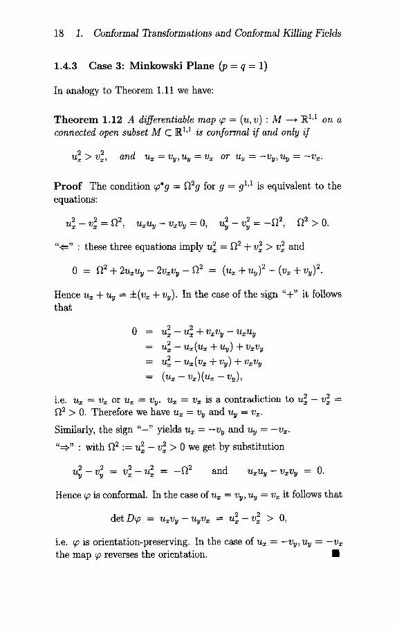
1 .4 .3 C a s e 3" M i n k o w s k i P l a n e (p = q = 1)
In analogy to T h e o r e m 1.11 we have:
T h e o r e m 1.12 A differentiable map ~ = (u, v) • M - - , R 1'1
connected open subset M C R 1'1 . i8 conformal i f and only i f
on a
Ux2 ~ Vx and U x ~ Vy~ Uy ~ V x O r U x ~ - -Vy~ Uy ~ - - V x .
P r o o f T h e condi t ion qo*g -- f/2g for g - g1,1 is equivalent to the
equat ions:
2 2 = g t 2 2 2 _f~2, f ~ 2 > 0 . U x - v x ~ U x U y - - V x V y - ~ O~ U y - - V y -~
2 gt2 2 2 and "¢=" • these three equat ions imply u~ = + v~ > v~
o = ~ + 2u~u~ - 2 ~ v ~ - a ~ = (u~ + u~) ~ - ( ~ + v~) ~
Hence ux + u u
t h a t
= :t:(v~ + vy). In the case of the sign "+" it follows
2 2 ---- U x - - U x q- V x V y - - U x U y
2 U y ) -~ U x - - U x ( U x -I- -t- V x V y
2 = u~ - u~(v~ + vu) + v~v~
= (u~ - v~)(u~ - ~ ) ,
2 2 i.e. u~ = v~ or u~ = vy. u~ = vx is a cont rad ic t ion to u x - v~ =
f~2 > 0. Therefore we have u~ = vy and uy = v~.
Similarly, the sign " - " yields u~ = - v ~ and uy = -v~ .
2 2 " ~ " • wi th ~2 := u~ - v~ > 0 we get by subs t i tu t ion
2 2 2 2 _ ~ 2 Uy - - Vy ~- V x - u x -~ and u~uy - v~vy = O.
Hence qo is conformal. In the case of u~ = vy, uy = v~ it follows t h a t
2 2 detDqo = u ~ v y - uyv~ = u ~ - v~ > 0,
i.e. qo is or ientat ion-preserving. In the case of u~
the m a p qo reverses the orientat ion.
- - - -Vy~ Uy - - - - V x
1
1.4 Classification of Conformal Transformations 19
The solutions of the wave equation A~ = n~ - ~yy = 0 in 1 + 1
dimensions can be written as
~(~, y) = f ( ~ + y) + g(~ - y)
with differentiable functions f and g of one real variable. Hence, any conformal Killing factor ~ has this form in the case of p = q = 1.
1 1 Let F and G be integrals of ~f and ~g, respectively. Then
x ( ~ , y) = (F(~ + y) + a ( ~ - y), F (~ + y) - a ( ~ - y))
is a conformal Killing field with X~,~+X~,, = g,~8. (This eventually completes the proof of the implication "¢=" in Theorem 1.6.) The associated one-parameter group (q0t) of conformal transformations consists of orientation-preserving maps with u~ - vy, uy = v~ for
~ = (u, v).
2 T h e C o n f o r m a l G r o u p
Definit ion 2.1 The conformal group Conf (R p'q) is the connected component containing the identity in the group of conformal diffeo- morphisms of the conformal compactification of R p'q.
In this definition, the group of conformal diffeomorphisms is con- sidered as a topological group with the topology of compact con- vergence.
2.1 Conformal Compact i f icat ion of R p,q
To study conformal transformations on open connected subsets M C R p'q, p + q >_ 2, a conformal compactification of I~ p'q is in-
troduced, in such a way that the conformal transformations be-
come everywhere-defined and bijective maps. Consequently, we search for a "minimal" compactification N p'q of R p,q with a nat- ural semi-Riemannian metric, such that every conformal transfor-
mation ~ : M --, R p'q has a continuation to N p'q as a conformal
diffeomorphism ~" N p'q --, N p'q and such that every conformal
diffeomorphism of N p'q is of this form (cf. Definition 2.5 for detail). Note that conformal compactifications in this sense only exist for p + q > 2 as we show in the sequel.
Let n = p4-q >_ 2. We use the notation <X>p,q := gP'q(x, x), x E R p'q. For short, we also write <x> - <x>p,q if p and q are evident from the context. IRp,q can be embedded into the (n 4- 1)-dimensional projective space IP~+I (R) by the map
z. R p,q ~ IP~+I(R),
1 - <x> xl x~ . • . . . . .
~ ' " ~ 2
Recall that IPn+I(I~) is the quotient
(R \ {o})/~ with respect to the equivalence relation
~~~'
1 +2
-" :- ~ - A ~ ' f o r a A E R \ { 0 } .
2.1 ConformM Compactif ication o f R p'q 21
Pn+l (R) can also be described as the space of one-dimensional sub- spaces of R ~+2. I?~+I(R) is a compact (n + 1)-dimensional dif- ferentiable manifold (cf. for example [Sch95]). If 7 " Rn+2\ {0} --* I?n+I(R) is the quotient map, a general point 7(~) E IPn+I(R),
_ (~o , . . . ,~+1) E R n+2, is denoted by ( ~ 0 . . . . . ~ + 1 ) . _ 7(~)
with respect to the so-called homogeneous coordinates. Obviously, we have
( ~ 0 . . . . . ~n+l) _. (/~0 . . . . . /~n+l) for all A e R \ {0}.
We are looking for a suitable compactification of RP,q. As a candi- date we consider the closure z(Rp,q) of the image of the differentiable embedding z" R p'q --, I?n+I(R).
R e m a r k 2 . 2 z(Rv,q) = N p,q, where
Np,q := { ( ~ o . . . . . ~n+l )E I~n+l(~)l (~)p+l,q+l--O}
P r o o f By definition of z we have ($(X))p+l,q+ 1 -- 0 for x ~ ~P'q, i.e.
?~(RP,q) C N p'q.
First of all, ( ~ o . . . . . ~+1) E N p'q \ z(R p'q) implies ~0 + ~=+1 = 0, since
( )~ - l (~ l , . . . ,~n ) ) __ ( ~ 0 . . . . . ~n+l )E ~(R p'q)
for )~ "-- ~o_[_ ~n+l ¢ 0. G i v e n (~o . . . . . ~n+l) E N p'q t h e r e
always exist sequences ek --* 0, 5k --* 0 with ek ¢ 0 ¢ 5k and 2~1ck q-c 2 = 2~n+1(~ k q-(~. For p _ 1 we have
Pk "= (~0 . ~1 + £k " ~2 . . . . . ~n . ~n+l .4_ ~k) C= N ~''q
Moreover, ~o + ~n+l _[_ (~k -- ¢~k # 0 implies Pk E z(RP'q). Finally, since Pk --* (~o. . ~+1) for k --, co it follows that (~o . . . . : ~n+l) E ?,(RP'q), i.e. N p'q C ~(Rv,q). m
We therefore choose N p'q as the underlying manifold of the confor- mal compactification. N p'q is a regular quadric in IP,+I(R). Hence it is an n-dimensional compact submanifold of IP~+I(R). N p'q con- tains ,(R v,q) as a dense subset.
We get another description of N p,q using the quotient map "y.
22 2. The Conformal Group
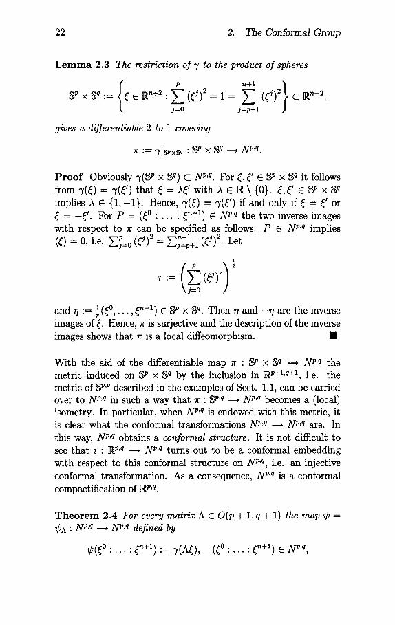
L e m m a 2.3 The restrict ion of 7 to the product of spheres
x sq "= {~ ~ R "+2" p n+l }
j=o j=p+ l
C Rn+2~
gives a differentiable 2-to-1 covering
71" "--" 7[$PxSq " SP X ~q ~ N p'q.
P r o o f Obviously 7 ( ~ x S q) c N p'q. For ~, ~' E S p x S q it follows from 7(~) = 7(~') that ~ = A~' with A E R \ {0}. ~, ~' E S p x S q implies A E {1 , -1} . Hence, 7(~) = 7(~') if and only if ~ = ~' or
= -~ ' . For P = ( ~ 0 . . . . . ~,+1) E N p'q the two inverse images with respect to 7r can be specified as follows: P E N p'q implies (~) - 0 i.e. ~-~=o (~j)2 ~-~n+l 2 , --" Z . . ~ j = p + l ( ~ J ) " Let
r °~
1
1 . . . , ~n+l sq. and the inverse and r / := 7(~0, ) E S p x Then r/ -r] are images of ~. Hence, r is surjective and the description of the inverse images shows that r is a local diffeomorphism. II
With the aid of the differentiable map 7r : S p x S q ---, N v,q the metric induced on ~ ' x S q by the inclusion in R v+l,q+l, i.e. the metric of ~"q described in the examples of Sect. 1.1, can be carried over to N p'q in such a way that r : SP 'q ~ N p'q becomes a (local) isometry. In particular, when N p'q is endowed with this metric, it is clear what the conformal transformations N p'q ---, N v'q are. In this way, N p'q obtains a conformal structure. It is not difficult to see that z : R p'q ---, N p'q turns out to be a conformal embedding with respect to this conformal structure on N p'q, i.e. an injective conformal transformation. As a consequence, N p'q is a conformal compactification of R v'q.
Theorem 2.4 For every matr ix A E O(p + 1, q + 1) the map ¢ =
CA" N p'q ~ N p'q defined by
~3(~0..... ~n+l).= 7(A~), ( ~ o . . . . . ~,+1) e N p'q,
2.1 Con[ormal Compactification o[R p'q 23
is a conformal transformation and a diffeomorphism. The inverse transformation ¢-1 = CA-~ is also conformal. The map A ~-, CA is not injective. However, CA = CA' implies A = A ~ or A = - A ' .
P r o o f For ~ e R~+2\ {0} with (x) = 0 and A e O(p + 1, q + 1) we have (A~) = g(A~, h~) = g(~, ~) = (~) = 0, i.e. ~/(h~) e N p'q. ~(A~) does not depend on the representative ~ as we can easily check: ~ ~ ~, i.e. ~ = r~ with r E R \ {0}, implies A ~ = rA~, i.e. A ~ ~ A~. Altogether, ¢ : N p'q --, N p'q is well-defined. Because of the fact that the metric on R p÷l'q÷l is invariant with respect to A, CA turns out to be conformal. For P E N p'q one calculates the conformal factor ~2 ~+1 j k 2. . (P) = ~-]~j=o (Ak~) if P is represented by
E S p x S q. (In general, A(S p x S q) is not contained in S v x S q, and the (punctual) deviation from the inclusion is described precisely by the conformal factor f~(P):
1
~(P) ~ A ( ~ ) e ~ x ~q for ~ E ~ X ~q and P - ~(~).)
Obviously, CA = ¢-A and ¢~1 = Ch-~. In the case CA = CA' for A,A' e O(p+ 1, q+ 1) we have ~/(h~) = ~(A'~) for all ~ e R ~+2 with (~) = 0. Hence, h = rh ' with r e R\{0}. Now A, A' e O(p+l, q+l) implies r - 1 or r - -1 . B
The requested continuation property for conformal transformations can now be formulated as follows:
Def in i t ion 2.5 Let ~ : M --, ~P,q be a conformal transformation on a connected open subset M C R p'q. Then ~" N p'q --, N p'q is called a conforrnal continuation of ~, if ~ is a conformal diffeo- morphism (with conformal inverse) and / f z (~ (x ) ) = ~(z(x)) for all x E M. In other words, the following diagram is commutative:
M • R p'q
A
Np,q ~ Np,q
24 2. The Conformal Group
2.2 The Conformal Group of R p'q for p + q > 2
T h e o r e m 2.6 Let n = p + q > 2. Every conformal transformation on a connected open subset M C R p'q has a unique conformal con- tinuation to N p'q. The group of all conformal transformations N p'q
N p,q is isomorphic to O(p+ 1, q+ 1)/{:kl}. The connected com- ponent containing the identity in this group - i.e., by Definition 2.1 the conformal group Conf (R p'q) - is isomorphic to SO(p+ 1, q+ 1).
Here, SO(p + 1, q + 1) is the connected component of the identity in O(p + 1, q + 1). SO(p + 1, q + 1) is contained in
{A E O(p+ 1, q + 1)[ detA = 1}.
However, it is, in general, different from this subgroup, e.g. for the case (p, q ) = (2, 1).
P r o o f It suffices to find continuations to N p'q of all the conformal transformations described in Theorem 1.9 and to represent these continuations by matrices A E O(p + 1, q + 1) according to Lemma 2.3.
1. Orthogonal transformations. The easiest case is the continua- tion of an orthogonal transformation ~(x) = A~x represented by a matrix A ~ E O(p, q). For the block matrix
l 1 0 0 / 0 A' 0 0 0 1
one obviously has A E O(p + 1, q + 1), because of ATrl A = ~, where 7/= diag(1, . . . , 1 , - 1 , . . . , - 1 ) is the matrix represent- ing gp+l'q+l. Furthermore,
h E SO(p+ 1,q+ 1) ~ h' E SO(p,q).
We define a conformal map ~" N p'q ---, N p'q by ~ "= ¢A, i.e.
(~(%~0..... %~n+l)_.~ (,~o. A, g . ~n+l)
2.2 The Conformal Group of IRp,v for p + q > 2 25
for ( { 0 . . . . . {,+1) e N p'q (cf. Theorem 2.4). For x 6 ]Rp,q we have
~(~(~)) = ( 1 - (x> " A ' x 2 . l+(x})2
(1 - <A'x> 1 + (A'x)) = ~ • A'~. ~ , ,
since A' e O(p, q) implies (x} = (A'x}. z(~o(x)) for all x e IR p'q.
Hence, ~ ( z ( x ) ) =
2. Translations. For a translation ~o(x) = x + c, c E IR ", one has the continuation
~ ( d . . . . . ~ -+~) := (~o _ (~,, c) - ~+ (c} • ~' + 2~+c
• ~+~ + <~', ~)+ ~+ <~))
for ( ~ 0 . . . . . ~,+1) E N p'q. Here,
= ~ + d ) and ~' = ( ~ 1 , . . . , ~ ) .
We have
~(~(x)) = (~ -<~ ,~) -~ .~+~ - - ~
1 and therefore since ~(z) + = ~,
~(~(~)) = (i - <~2 + ~> " x + c " l + < ~ + ~ > )
2 = ~(~(~))"
Since @ = Ca with A E SO(p+l, q-t-l) can be shown as well, is a well-defined conformal map, i.e. a conformal continuation of ~o. The matrix we look for can be found directly from the definition of ~. It can be written as a block matrix:
i i-l<cl 1 A~= c E~ ½ <~> (~'~)~ i + ½ <~)
Here, E~ is the (n × n) unit matrix and
~' = diag(l,..., i, - I , . . . , - I )
26 2. The Conformal Group
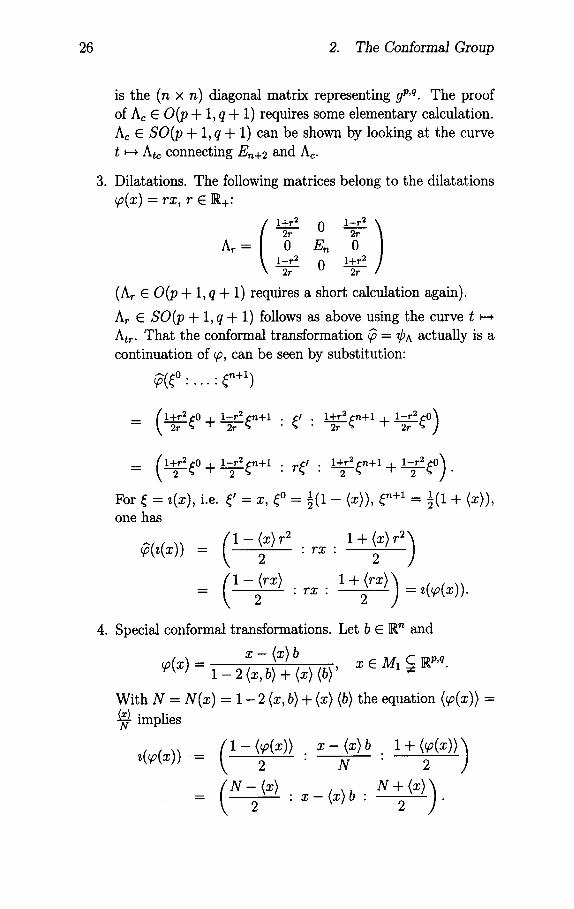
is the (n x n) diagonal matrix representing gP'q. The proof of Ac E O(p + 1, q + 1) requires some elementary calculation. A~ E SO(p + 1, q + 1) can be shown by looking at the curve t ~ At~ connecting E~+2 and A~.
3. Dilatations. The following matrices belong to the dilatations ~o(x) = rx, r E R+:
i?,
l't-r2 0 l--r2 / 2r 2r 0 E~ 0
l-r2 0 l+r2 2r 2r
(A~ E O(p + 1, q + 1) requires a short calculation again).
A~ E SO(p + 1, q + 1) follows as above using the curve t At,.. That the conformal transformation ~ = CA actually is a continuation of ~, can be seen by substitution:
~ ( ~ 0 . . . . . ~n+l)
1 +r 2 ,cO 1-r 2 ~n-{- 1--r 2 riO i . ~, . i+~2 ~ , + i + - ~ - - _ 2r ]
__ (l~r__~2~0~_ ~ ~ n ÷ l . r~' • l+;2~n+l-~ - l~r--~2~0).
For ~ = z(x) i.e. ~ '= x ~o 1 ~+1 1 , , = 5 ( 1 - (x ) ) , = 5(1 + (x ) ) , one has
~(z(x)) = (X-(x)2 r2 • rx • 1+(x)2 r2)
( 1 - (rx) 1 + <rx)) = i • r ~ • 2 = ~(~(~))
4. Special conformal transformations. Let b E IR ~ and
(p(X) --- 1 -- 2 ( x , b ) -~- (x) (b) ' x e U l C ]l~p,q.
With N = N(x) = 1 - 2 (x, b) + (x) (b) the equation (~(x)) = (~) implies N
(1 x <x>b 1 + 2 N <x>
= ~ • ~ - ( ~ ) b • 2 "
2.2 The Conformal Group o? R p'q for p + q > 2 27
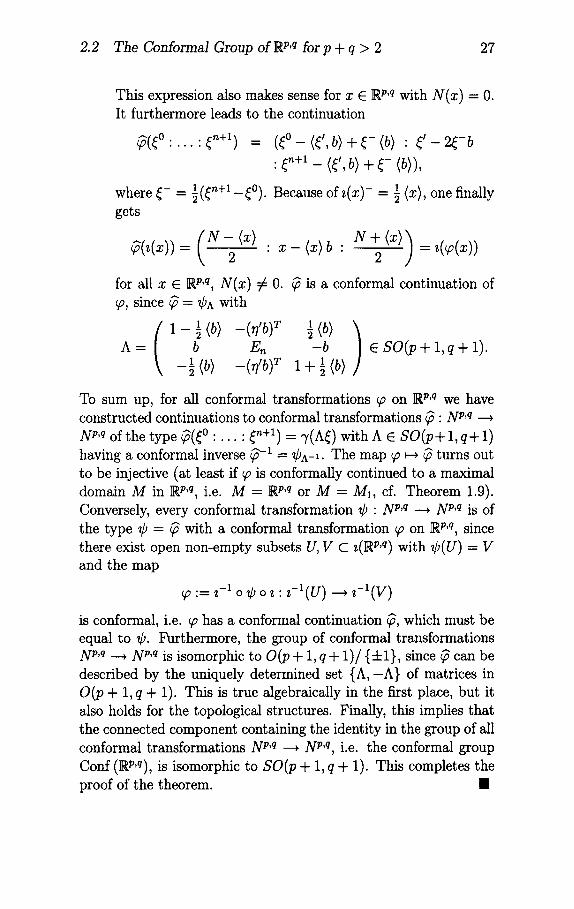
This expression also makes sense for x 6 RP,q with N(x) = O. It furthermore leads to the continuation
~(~0 . . ~ + 1 ) = (~0 _ (~,, b) + ~- (b) • ~ ' - 2~-b
• b) + @), 1 (~n+i - 1 where ~- = 5 _ ~0). Because of z(x) = 5 ix), one finally
gets
~(z(x))= ( N - ( x ) " x - (x) b " N 2(x))=z(~v(x) )
for all x E R p'q, N(x) ~ O. ~ is a conformal continuation of ~, since ~ = CA with
A = En E S O ( p + 1, q + 1). -½ (b) 1 + ½ (b)
To sum up, for all conformal transformations ~ on Rp,q we have constructed continuations to conformal transformations ~" NP,q --. N v'q of the type ~ ( ~ 0 . . . . . ~+1) = 7(A~) with A 6 SO(p+ 1, q+ 1) having a conformal inverse ~-1 = ¢^_~. The map ~v ~ ~ turns out to be injective (at least if ~ is conformally continued to a maximal domain M in Rv,q, i.e. M = Rv,q or M = M1, cf. Theorem 1.9). Conversely, every conformal transformation ¢ : NP'q ~ NP'q is of the type ¢ = ~ with a conformal transformation ~v on R v'q, since there exist open non-empty subsets U, V C z(Rp,q) with ¢(U) = V and the map
.__ $-1 o ~) o ~ " ~ , - I ( u ) ----4 ~ - l ( v )
is conformal, i.e. ~ has a conformal continuation ~, which must be equal to ¢. Furthermore, the group of conformal transformations N p'q ~ N v'q is isomorphic to O(p + 1, q + 1)/{4-1}, since ~ can be described by the uniquely determined set {A,-A} of matrices in O(p + 1, q + 1). This is true algebraically in the first place, but it also holds for the topological structures. Finally, this implies that the connected component containing the identity in the group of all conformal transformations NP'q ~ NP'q, i.e. the conformal group Conf (Rp,q), is isomorphic to SO(p + 1, q + 1). This completes the proof of the theorem, m
28 2. The Conformal Group
2.3 T h e C o n f o r m a l G r o u p of R 2'°
By Theorem 1.11, the orientation-preserving conformal transfor- mations ~ : M --, R 2'° ~ C on open subsets M c R 2'° ~ C are
exactly those holomorphic functions with nowhere-vanishing deriva- tive. This immediately implies, that a conformal compactification according to Remark 2.2 and Definition 2.5 cannot exist, because there are many non-injective conformal transformations, e.g.
C \ { 0 } - - - , C , z ~ z k, f o r k e Z \ { - 1 , 0 , 1 } .
There are also many injective holomorphic functions without a suit- able holomorphic continuation, like
z ~ z 2, z E { w E C ' R e w > O } ,
or the principal branch of the logarithm on the plane that has been slit along the negative real axis C \ { - x • x E R+}. However, there is a useful version of the ansatz from Sect. 2.2 for the case p - 2, q - 0, which leads to a result similar to Theorem 2.6.
Def in i t ion 2.7 A global conformal transformation on R 2'° is an injective conformal transformation, which is defined on the entire plane C with at most one exceptional point.
The analysis of conformal Killing factors (cf. Sect. 1.4.2) shows, that the global conformal transformations and all those conformal transformations, which admit a (necessarily unique) continuation to a global conformal transformation, are exactly the transformations, which have a linear conformal Killing factor or can be written as a composition of a transformation having a linear conformal Killing factor with a reflection z ~ ~. Using this result, the following theorem can be proven in the same manner as Theorem 2.6.
T h e o r e m 2.8 Every global conformal transformation ~ on M C C has a unique conformal continuation ~" N 2'° --, N 2'°, where
= ~aA with A E 0(3, 1). The group of conformal diffeomorphisms ¢ " N 2,° --, N 2,° is isomorphic to 0(3, 1)/{:i:1} and the connected component containing the identity is isomorphic to S0(3, 1).
2.3 The Conformal Group of lR 2'° 29
In view of this result, it is justified to call the connected component containing the identity the conformal group Conf(R 2,°) of R 2'°. An- other reason for this comes from the impossibility of enlarging this group by additional conformal transformations discussed below.
A comparison of Theorems 2.6 and 2.8 shows the following excep- tional situation of the case p + q > 2: every conformal transfor- mation, which is defined on a connected open subset M C R p'q, is injective and has a unique continuation to a global conformal transformation. (A global conformal transformation in the case of ]R p,q, p + q > 2, is a conformal transformation ~ : M ---. IR p,q, which is defined on the entire set IR p,g with the possible exception of a hy- perplane. By the results of Sect. 1.4.2, the domain M of definition of a global conformal transformation is M = IR p'q or M = M1, see (3).)
Now, N 2'° is isometrically isomorphic to the 2-sphere S 2 (in general, one has N p'° ~ S p, since S p × S ° = S p × {1 , -1}) and hence N 2'° is conformally isomorphic to the Riemann sphere P := PI(C). A M5bius transformation is a holomorphic function ~, for which there is a matrix
a b ) az+b c d ESL(2 , C) such that ~ ( Z ) = c z + d , cz+d¢O.
The set Mb of these Mhbius transformations is precisely the set of all orientation-preserving global conformal transformations (in the sense of Definition 2.7). Mb forms a group with respect to composition (even though it is not a subgroup of the bijections of C). For the exact definition of the group multiplication of and ¢ one usually needs a continuation of ~ o ¢ (cf. Lemma 2.9). This group operation coincides with the matrix multiplication in SL(2, C). Hence, Mb is also isomorphic to the group PSL(2, C) : - SL(2, C) /{+1} . Moreover, by Theorem 2.8, Mb is isomorphic to the group of orientation-preserving and conformal diffeomorphisms of N 2,° -~ I?, i.e. to the group Aut(I?) of biholomorphic maps ¢" I? ---, I? of the Riemann sphere I?. This transition from the group Mb to Aut(I?) using the compactification C ~ I? has been used as a model for the compactification N v'q of IR p'q and the respective Theorem 2.6. Theorem 2.8 says even more: Mb is also isomorphic to the proper Lorentz group SO(3, 1). An interpretation of the
30 2. The Conformal Group
isomorphism Aut(IP) =~ S0(3, 1) from a physical viewpoint was given by Penrose, cf. e.g. [Sch95, p. 210]. In summary, we have
SL( C)"~ ( ) SO( ) f( ) Mb "~ P 2, = A u t I P "~ 3,1 ~ C o n R 2'° ~ " •
Throughout physics texts on two-dimensional conformal field the- ory one finds the claim that the group ~; of conformal transforma- tions on R 2'° is infinite dimensional, e.g.
[BPZ84, p. 335] "The situation is somewhat better in two dimensions. The main reason is that the conformal group is infinite dimensional in this case; it consists of the conformal analytical transformations..." and later ". . . the conformal group of the 2-dimensional space con- sists of all substitutions of the form
m
z
u
where ~ and ~ are arbitrary analytic functions."
[FQS84, p. 4 2 0 ] "Two dimensions is an especially promising place to apply notions of conformal field in- variance, because there the group of conformal transfor- mations is infinite dimensional. Any analytical function mapping the complex plane to itself is conformal."
[GO89, p. 333] "The conformal group in 2-dimensional Euclidean space is infinite dimensional and has an alge- bra consisting of two commuting copies of the Virasoro algebras."
At first sight, the statements in these citations seem to be totally wrong. For instance, the class of all holomorphic (i.e. analytic) functions z ~ ~(z) does not form a g roup- in contradiction to the first citation - since for two general holomorphic functions f : U V, g : W ~ Z with open subsets U, V, W, Z C C, the composition g o f can be defined at best if f(U) N W 7~ 0. Moreover, the non- injective holomorphic functions f are not invertible. If we restrict ourselves to the set J of all injective holomorphic functions the
2.3 The ConformM Group of R 2'° 31
composition cannot define a group structure on J because of the fact that f (U) C W will, in general, be violated; even f(U) N W = q} can occur. Of course, J contains groups, e.g. Mb and the group of biholomorphic f : U --~ U on an open subset U C C. However, these groups Aut(U) are not infinite dimensional, they are finite-dimensional Lie groups. If one tries to avoid the difficulties of f (U)N W = q} and requires - as the second citation [FQS84] seems to suggest- the transformations to be global, one obtains the finite- dimensional MSbius group. Even if one admits more then one-point singularities, this yields no larger group than the group of MSbius transformations, as the following lemma shows:
L e m m a 2.9 Let f :C \ S --, C be holomorphic and injective with a discrete set of singularities S C C. Then, f is a restriction of a MSbius transformation. Consequently, it can be holomorphicaUy continued on C or C \ {p}, p E S.
P r o o f By the theorem of Casorati-Weierstrat], the injectivity of f implies that all singularities are poles. Again from the injectivity it follows by the Riemann removable singularity theorem, that at most one of these poles is not removable and this pole is of first order, m
The omission of larger parts of the domain or of the range also yields no infinite-dimensional group: doubtless, Mb should be a subgroup of the conformal group G. For holomorphic f : U ---, V, such that C \ U contains the disc D and C \ V contains the disc D ~, there always exists a MSbius transformation h with h(V) C D' (inversion with respect to the circle OD'). Consequently, there is a MSbius transformation g with g(Y) C D. But then Mb t.J {/} can generate no group, since f cannot be composed with g o f because of (g o f(U)) N U = 0. A similar statement is true for the remaining / e J . As a result, there can be no infinite-dimensional conformal group G for the Euclidean plane. What do physicists mean when they talk about an infinite-dimensional conformal group? The misun- derstanding seems to be that physicists mostly think and calculate infinitesimally, while they write and talk globally. Many state- ments become clearer, if on replaces "group" with "Lie algebra"
32 2. The Conformal Group
and "transformation" by "infinitesimal transformation" in the re- spective texts. If, in the case of the Euclidean plane, one looks at conformal Killing fields instead of conformal transformations (cf. Sect. 1.4.2), one immediately finds many infinite-dimensional Lie algebras within the collection of conformal Killing fields. In partic- ular, one finds the Witt algebra. In this context, the Witt algebra W is the complex vector space with basis (L~)~z, L~ "= - z ~+ld
dz or L~:= z 1 -nd (cf. Sect. 5.2), and the Lie bracket
[Ln, L~] = (n - m)Ln+~
(cf. Sect. 5). In two-dimensional conformal field theory usually only the infinitesimal conformal invariance of the system under con- sideration is used. This implies the existence of an infinite number of independent constraints, which yields the exceptional feature of two-dimensional conformal field theory.
Another explanation for the claim that the conformal group is in- finite dimensional and can perhaps be found if one looks at the Minkowski plane instead of the Euclidean plane. This is not the point of view in most papers on conformal field theory, but it fits in with the type of conformal invariance naturally appearing in string theory (cf. Sect. 8). Indeed, conformal symmetry was in- vestigated in string theory, before the actual work on conformal field theory had been done. For the Minkowski plane, there is re- ally an infinite-dimensional conformal group, as we will show in the next subsection. The associated complexified Lie algebra is again essentially the Witt algebra (cf. Sect. 5.1).
Hence, on the infinitesimal level the cases (p, q) = (2, 0) and (p, q) = (1, 1) seem to be quite similar. However, in the interpretation and within the representation theory there are differences, which we will not discuss here. We shall just mention that the Lie algebra ~[(2, C) belongs to the Witt algebra in the Euclidean case (as the Lie algebra of Mb generated by L_I, L0, L1), while in the Minkowski case it is only generated by complexification of ~[(2, R) .
2.4 The Conformal Group of ]l~ 1'1
By Theorem 1.12 the conformal transformations ~ on domains M C R 1'1 are precisely the maps ~ = (u, v) with u~ = vy, uy = v~ or
2.4 The Conformal Group of RI,1 33
2 2 For M = N 1,1 one u~ = -vy, uy = -v~, and, in addition, u~ > v~. has the following description of the global orientation-preserving conformal transformations:
Theorem 2.10 For f e C ~ (R) let f+ e C °~ (R 2, R) be defined by f± (~, y) := : (~ + y). Th~ map
¢ . c ~ (R) × c ~ (R) , c ~ (R ~, R ~) 1
(f , g) , , 5 (f + + g-, f + - g-)
has the following properties:
1. im (I) = { (u, v) e C ~ (R 2, R2) • ux = vy, uy = vx }.
2. O( f, g) conformal ~ f ' > O, g' > 0 or f ' < O, g' < O.
3. (I)(f,g) bijective ..v--5. f and g bijective.
~. O( f o h, g o k) = O( f , g) o O(h, k) for f , g, h, k e C°~(R).
Hence, the group of orientation-preserving conformal diffeomor- phisms ~" R 1,1 ---, R 1'1 is isomorphic to the group
(Diff+ (R) x Diff+ (R)) U (Diff_ (R) x Diff_ (R)).
The group of all conformal diffeomorphisms consists of four compo- nents. Each component is homeomorphic to Diff+(R) x Diff+(R). Diff+(R) denotes the group of orientation-preserving diffeomorph- isms R ---, R with the topology of uniform convergence on compact subsets K C R in all derivatives.
P r o o f
1. Let (u, v) = q~(f, g). From
1 g . ~ g . u~ = ~(f; + ) ~ = ~(f:,- )
1 g . 1 g . v~ = ~ ( : ; - ) v~ = ~ ( f ; + )
it follows immediately that u~ = vy, uy = v~. Conversely, let
(~, v) ~ c°°(R2, R 2)
34 2. The Conformal Group
w i t h u , = vy, u~ = v,. T h e n u , , = v w = u~y. Since a solution of the one-dimensional wave equation u has the form
1 (X, y)) with f, e C °° u(x, y) = 5 (f+ (x, y) + g_ g (R). Because 1 g,_ 1 g,_ , o f v ~ = u y = 5 ( f ~ - ) a n d v y = u ~ = ~ ( f ~ + ) we have
1 v = ~ ( f + - g_) where f and g possibly have to be changed by a constant.
2 2 ~ / 2. For (u, v) = ~( f , g) one has u~ - v~ = f + g . Hence
2 2 , , f,g, u , - v , > O ~ f+g_>O ~ > 0 .
3. Let f and g be injective. For ~v = O(f, g) we have:
~(x, y) = ~v(x', y') implies
f (x + y) + g(x - y)
f (x + y) - g(x - y)
= + ¢) + ¢),
= + ¢) - ¢).
Hence, f ( x + y) = f (x' + y') and g(x - y) = g(x' - y'), i.e. x + y = x ' + y ' and x - y = x ' - y ' . This implies x = x', y = y'. So ~ is injective if f and g are injective. From the preceding discussion one can see: if ~v is injective then f and g are injective, too. Let now f and g be surjective and ~v = (I)(f, g). For (~, r/) e N 2 there exist s, t E N with f (s) = ~ + ~1, g(t) = ~ - r/. Then qv(x,y) = (~,r/) with x ' = 5~(s + t), Y := 51( s - t). Conversely, the surjectivity of f and g follows from the surjectivity of ~.
4. With ~ = O(f, g), ¢ = (I)(h, k) we have ~vo¢ = ½(f+ o~b+ g_ o '(h+ +k_) + k_)) = ¢, f+ o ¢ - g - o¢) and f+ o ¢ = f(~
f o h+ = ( f o h)+, etc. Hence
1 : o ¢ = oh)++(gok)_, ( f oh)+-(gok)_) = ¢ ( f oh, gok).
II
As in the case p -- 2, q = 0, there is no theorem similar to The- orem 2.6. For p = q = 1, the global conformal transformations need no continuation at all, hence a conformal compactification is not necessary. In this context it would make sense to define the
2.4 The Conformal Group of ]R1,1 35
conformal group of ~1,1 simply as the connected component con- taining the identity of the group of conformal transformations R 1'1 ---, R 1,1. This group is very large; it is by Theorem 2.10 isomorphic to Diff+ (]~) x Diff+ (R).
However, for various reasons one wants to work with a group of transformations on a compact manifold with a conformal structure. Therefore, one replaces R 1'1 with S 1'1 in the sense of the conformal compactification of the Minkowski plane which we described at the beginning (cf. Sect. 1.2):
R 1'1 ~ S 1'1 = S X S C R 2'0 X ~0,2.
In this manner, one gets the conformal group Conf(R 1'1) as the connected component containing the identity in the group of all conformal diffeomorphisms S 1'1 ---, S 1'1. Of course, this group is denoted by Conf(S 1'1) as well.
In analogy to Theorem 2.10 one can describe the group of orientation- preserving conformal diffeomorphisms S 1'1 ---, S 1'1 using Diff+(S) and Diff_(S) (one simply has to repeat the discussion with the aid of the 2It-periodic functions). As a consequence, the group of orientation-preserving conformal diffeomorphisms S 1'1 --~ S 1'1 is isomorphic to the group
(Diff+ (S) x Diff+ (S)) U (Diff_ (S) × Diff_ (S))
Corol la ry 2.11 Conf(R 1,1) ~ Diff+ (S) x Diff+ (S).
In the course of investigation of classical field theories with con- formal symmetry Conf(R 1'1) and its quantization one is therefore interested in the properties of the group Diff+ (S) and its associated Lie algebra Lie Diff+ (S). The complexification of this algebra con- tains the Witt algebra W mentioned at the end of Sect. 2.3. For the quantization of such classical field theories the symmetry groups or algebras Diff+(S), Lie Diff+(S) and W have to be replaced with suitable central extensions. We will explain this procedure in the following two sections. In particular, this is the way the Virasoro algebra is introduced as a nontrivial central extension of W (cf. Sect. 5).
3 Central Extensions of Groups
3.1 Central Extensions
In this section let A be an abelian group and G an arbitrary group.
Definition 3.1 An extension of G by the abelian group A is given by an exact sequence of group homomorphisms
1 , A " E ~G >1.
Exactness of the sequence means that the kernel of every map in the sequence equals the image of the previous map. Hence the sequence is exact if and only if ~ is injective, r is surjective and ker 7r =
im ~ (~ A).
The extension is called central if the image ~ (A) of A is in the center of E, i. e.
a e A,b e E =~ ~ (a)b = b~(a).
Examples:
• A trivial extension has the form
1 , A i pr2> ~ A x G G >1,
where A x G denotes the product group and where i • A --. G is given by a ~ (a, 1). This extension is central.
• An example for a non-trivial central extension is the exact
sequence
1 ~Zk ~ E = U ( 1 ) ~ U ( 1 ) ;1
with ~ (z) "= z k for k E N, k >_ 2. This extension cannot
be trivial, since E = U(1) and Zk x U(1) are not isomorphic. Another argument for this uses the fact - known for example from function t h e o r y - that a homomorphism T" U(1) ~ E
with ~ OT --- idv(1) does not exist, since there is no global k-th
root.
3.1 Central Extensions 37
• Let V be a vector space over a field K. Then
, K x idv----,GL(V) '~, PGL(V) ,1
is a central extension by the (commutative) multiplicative group g × = g \ {0} of units in g . Here, the projective linear group PGL(V) is simply the factor group PGL(V) = G L ( V ) / K x.
The main example in the context of quantization of symme- tries is the following: Let ]HI be a Hilbert space over C with inner product ( , ) and let ~ - IP (]HI) be the projective space of one-dimensional linear subspa~es of IHI, i.e.
.= (H \ {0} ) /~ ,
with the equivalence relation
f ,,~ g . ~ 3A E C x • f = Ag for f, g E ]HI.
is the space of states in quantum physics, i.e. the quantum mechanical phase space.
Using the inner product (., .) of the Hilbert space ]E one de- fines the set U(]E) of unitary operators on ]HI. U(]HI) is the set of all C-linear bijective maps U" H ---, ]HI with the following property:
f, g E ]I"]I ~ (U f , Ug) = (f , g) .
It is easy to see that the inverse U -1 : ]I-lI ---, IE of a unitary operator U :]E ---, IE is unitary as well and that the compo- sition U o V of two unitary operators U, V is always unitary. Hence, the composition of operators defines the structure of a group on U(IE). U(]HI) with this structure is called the unitary group of IE.
Let 7 : ]HI \ {0} ~ IP be the canonical map into the quotient spaceP(H) = ( ] E \ { 0 } ) / ~ . Let ~ = 7 ( f ) and ¢ = 7 ( g ) be points in the projective space P with f, g E ]HI. We then define the "transition probability" as
llfll'llgll "
38 3. Central Extensions of Groups
Furthermore, using 5 we define the group Aut(F) of projective automorphisms to be the set of bijective maps T" F ~ F with the property
(T~, T¢) = 5 (~, ¢) for ~, ¢ e IP,
where the group structure is again given by composition. Hence, Aut(IP) is the group of transformations of IP preserving the transition probability.
For every U e U(]HI) we define a map ~(U): IP ---, IP by
. =
for all ~ = 7(f) E IP with f E IHI. It is easy to show that ~(U)" IP ---. IP is well-defined and belongs to Aut(IP). This is not only true for unitary operators, but also for the so-called anti-unitary operators V, i.e. for the JR-linear bijective maps V" ]HI ~ ]HI with
(V f, Vg} = ( f , g) , V(i f ) - - i V ( f )
for all f, g e ]HI. Note that ~" U(H) ---. Aut(IP) is a homo- morphism of groups.
The following theorem contains a complete characterization of the projective automorphisms:
T h e o r e m 3.2 (Wigner [Wig31], Chap. 20, Appendix). For every transformation T E Aut(]P) there is a unitary or an anti-unitary operator U with T = ~(U).
The elementary proof of Wigner has been simplified by Bargmann [Bar64].
Let U(IP) "= ~ (U(EI)) C Aut(lP).
Then U(IP) is a subgroup of Aut(IP). In the following we are in- terested in the central extension of the group U(IP) given by the homomorphism ~:
3.2 Quantization of Symmetries 39
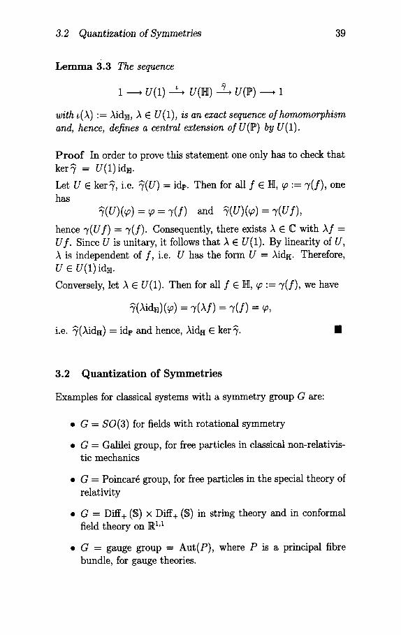
L e m m a 3.3 The sequence
A
1 ~U(1) ~, U(H) ~ , U ( P ) ,1
with L()~) :-- )rids, )~ e U(1), is an exact sequence of homomorphism and, hence, defines a central extension of U(P) by U(1).
Proof In order to prove this statement one only has to check that ker ~ = U(1) idH.
Let U E ker~, i.e. ~(U) = idr. Then for all f E H, ~ "= 7(f) , one has
~(U)(~) = ~ = 7(f) and ~(U)(~) = 7(U f),
hence 7(U f) = 7(f). Consequently, there exists A E C with )~f = Uf. Since U is unitary, it follows that )~ E U(1). By linearity of U,
is independent of f , i.e. U has the form U = Aids. Therefore, U E U(1)ids.
Conversely, let A e U(1). Then for all f e H, ~ "= 7(f) , we have
~(Aid~)(~) - ~(Af) - ~(f) - ~,
i.e. ~()~ids) - idp and hence, Aids E ker~. m
3.2 Quant izat ion of Symmetr ies
Examples for classical systems with a symmetry group G are:
• G = SO(3) for fields with rotational symmetry
• G - Galilei group, for free particles in classical non-relativis- tic mechanics
• G - Poincar6 group, for free particles in the special theory of relativity
• G = Diff+ (S) × Diff+ (S) in string theory and in conformal field theory on R 1'1
• G = gauge group = Aut(P), where P is a principal fibre bundle, for gauge theories.
40 3. Central Extensions of Groups
All these groups are topological groups in a natural way. A topo- logical group is a group G equipped with a topology, such that the group operation G × G --, G, (g, h) ~ gh, and the inversion map G --, G, g ~ g-i , are continuous. The first three examples are finite-dimensional Lie groups, while the last two examples are infinite-dimensional Lie groups (modeled on Fr~chet spaces). The topology of Diff+(S) will be discussed shortly at the beginning of Sect. 5.
After quantization of the symmetry, a homomorphism
T" G --, U(I?)
remains, which is continuous for the strong topology on U(P) (see below for the definition of the strong topology). This property cannot be proven - it is, in fact, an a s s u m p t i o n concerning the quantization procedure. The reasons for making this assuption are the following. It seems to be evident from the physical point of view that each classical symmetry g E G should induce after quan- tization a transformation T(g) : IP --, P of the quantum mechanical phase space. Again by physical arguments, T(g) should preserve the transition probability, since 5 i s - at least in the case of classical mechanics - the quantum analogue of the symplectic form which is preserved by g. Hence, by these considerations, one obtains a map T : G --, Aut(lP). In addition to these "physical" require- ments it is simply reasonable and convenient to assume that T has to respect the natural additional structures on G and Aut(lP), i.e. to be a continuous homomorphism. For connected G this implies T(G) C hut(I?).
Def in i t ion 3.4 Strong topology on U(N)" Typical neighborhoods of Uo E U(]E) are the sets
{u e u ( s ) IIUo (fo)- u (/o)11 < with fo E IE, e > O.
These neighborhoods form a subbasis of the strong topology. The strong topology on U (H) is not metrizable. On U (~) a topology (the quotient topology) is defined using the map ~" U(IE) --~ U(IP)"
B c g(I~) open :., ;. ~-1 ( B ) C U(][-]I) open.
3.2 Quantization of Symmetries 41
The strong topology can be defined on any subset
M C B(]HI)"= { B" ]HI ---, IHIIB is R-linear and bounded}
of JR-linear continuous operators, hence in particular on
M~ = { U" ][-]I ---, IHI[U unitary or anti-unitary}.
In the same way as above a topology on Aut(?) is induced by ~" M~ Aut(IP) (cf. Wigner's Theorem 3.2). This topology on Aut(IP)
(or U(IP)) is called the strong topology as well.
When quantizing a classical symmetry group the following question arises: given a continuous homomorphism T : G ~ U(~*), does there exist a continuous homomorphism S : G ~ U(]HI), such that the following diagram commutes?
G
T
1 . U ( 1 ) ~ --U(]HI) ^~ U(IP) . 1 ,7
The answer is, no; such a lifting does not exist in general. Therefore, it is, in general, not possible to take G as the quantum mechanical symmetry group in the sense of a continuous representation S • G ~ U(]HI). However, a lifting exists with respect to the central extension of the universal covering group of the classical symmetry group. (Here and in the following, the universal covering group of a connected Lie group G is the (up to isomorphism) uniquely determined connected and simply connected universal covering G of G with its Lie group structure.) This is well-known for the rotation group SO(3):
E x a m p l e 3.5 Transition from SO(3) to the simply connected 2- to-1 covering group SU(2)" for every continuous homomorphism T " SO(3) ~ U(IP) one has the following commutative diagram:
1 • U(1) - -U(1)x SU(2) -- SU(2) . 1
1 , U(1) --U(IHI) ^ , U(P) ~ 1 .y
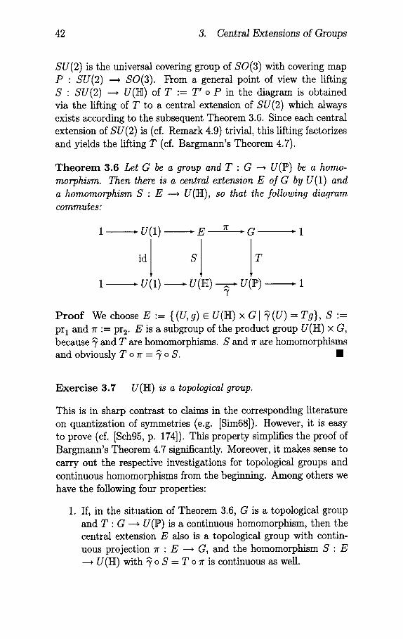
42 3. Central Extensions of Groups
SU(2) is the universal covering group of SO(3) with covering map P : SU(2) ---, SO(3). From a general point of view the lifting S : SU(2) ---, U(H) of T : - T' o P in the diagram is obtained via the lifting of T to a central extension of SU(2) which always exists according to the subsequent Theorem 3.6. Since each central extension of SU(2) is (cf. Remark 4.9) trivial, this lifting factorizes and yields the lifting T (cf. Bargmann's Theorem 4.7).
T h e o r e m 3.6 Let G be a group and T • G ~ U(P) be a homo-
morphism. Then there is a central extension E of G by U(1) and a homomorphism S • E ~ U(]E), so that the following diagram
commutes"
1 , U(1) ~ E
id S
1 u(1) u(s)
"G ~1
^ , U(P) , 1 7
P r o o f We choose E "= { (U, g ) e U(]HI) x G [ ~ ( U ) = Tg}, S "=
pr I and r := pr 2. E is a subgroup of the product group U(iE) x G, because ~ and T are homomorphisms. S and r are homomorphisms and obviously T o r = ~ o S. m
Exercise 3.7 U(H) is a topological group.
This is in sharp contrast to claims in the corresponding literature on quantization of symmetries (e.g. [Sim68]). However, it is easy to prove (cf. [Sch95, p. 174]). This property simplifies the proof of Bargmann's Theorem 4.7 significantly. Moreover, it makes sense to carry out the respective investigations for topological groups and continuous homomorphisms from the beginning. Among others we have the following four properties:
1. If, in the situation of Theorem 3.6, G is a topological group and T : G ---. U(P) is a continuous homomorphism, then the central extension E also is a topological group with contin- uous projection r • E ---. G, and the homomorphism S" E
U(H) with ~ o S = T o r is continuous as well.
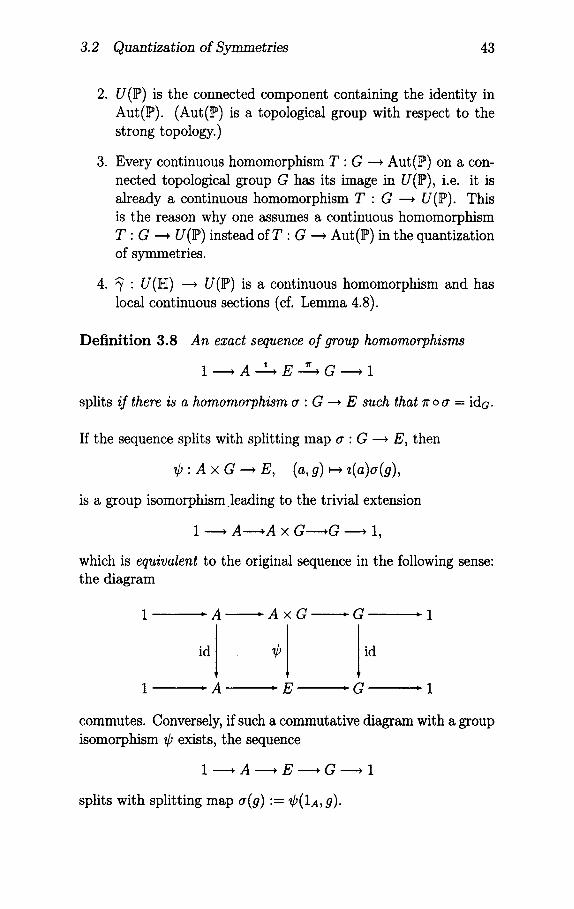
3.2 Quantization of Symmetries 43
2. U(P) is the connected component containing the identity in Aut(P). (Aut(P) is a topological group with respect to the strong topology.)
3. Every continuous homomorphism T : G --~ Aut(P) on a con- nected topological group G has its image in U(P), i.e. it is already a continuous homomorphism T : G --~ U(P). This is the reason why one assumes a continuous homomorphism T : G --, U(P) instead of T : G --, Aut(P) in the quantization of symmetries.
4. ~" U(]E) ---, U(P) is a continuous homomorphism and has local continuous sections (cf. Lemma 4.8).
Definition 3.8 An exact sequence of group homomorphisms
1 A ~ E ~G ~1
splits i f there is a homomorphism a • G ~ E such that r o a = idG.
If the sequence splits with splitting map a" G ---, E, then
¢ " A × G --~ E, (a, g ) ~ z(a)a(g),
is a group isomorphism.leading to the trivial extension
1 ~ A---~A × G - - * G ~ 1,
which is equivalent to the original sequence in the following sense: the diagram
1 : A ~ A x G ~G , 1
id ¢ id
1 ~A , E ' G ~1
commutes. Conversely, if such a commutative diagram with a group isomorphism ¢ exists, the sequence
1 ~A ~E , G ,1
splits with splitting map a ( g ) : = ¢(1A, g).
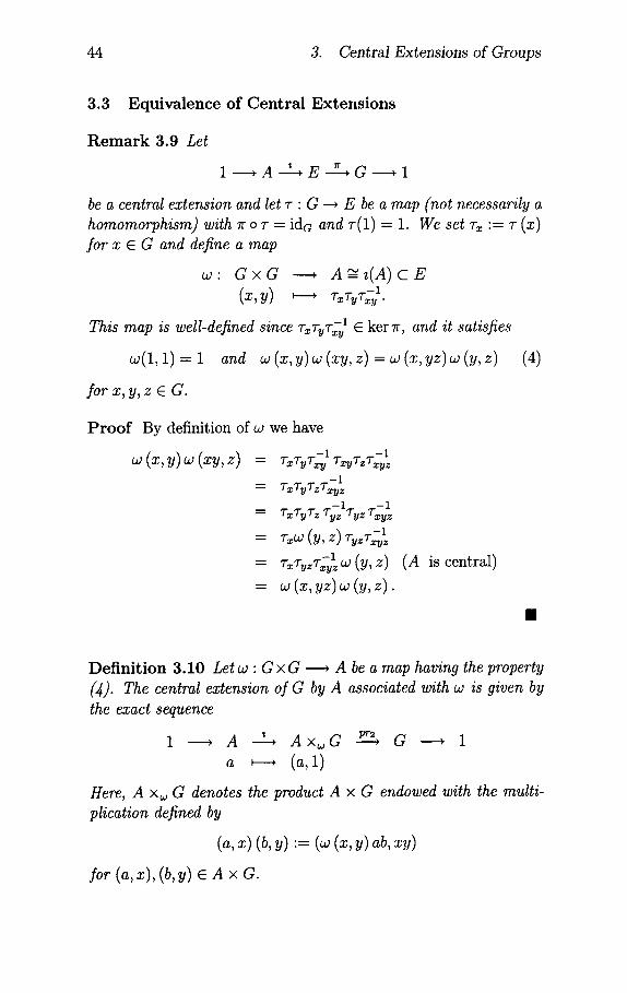
44 3. Central Extensions of Groups
3.3 Equivalence of Central Extensions
R e m a r k 3.9 Let
1 ~ A - - ~ E " ~ G ~1
be a central extension and let T • G ---* E be a map (not necessarily a homomorphism) with r o T = ida and T(1) = 1. We set T~ "= T (X) for x 6 G and define a map
02 " G × G ) A~-~(A) C E (~ ,y ) , ~ ~ ~
This map is well-defined since TzTyT~ 1 6 ker r , and it satisfies
w(1, 1) = 1 and w (x, y)w (xy, z) = w (x, yz) w (y, z) (4)
for x, y, z 6 G.
P r o o f By definition of w we have
TxTyT~I -I - - T x y T z T x y z
- 1 "-- T x T y T z T x y z
= ~ ~ z % z ~ z ~ - ~ z = ~ (y, z)~z~-~l~
= ~ ~ ; ~ l z ~ (y, z)
= ~ (~, y z ) ~ (y, z ) .
(A is central)
m
Definition 3.10 Let w • G × G ~ A be a map having the property (~). The central extension of G by A associated with w is given by
the exact sequence
1 ) A ' pr2) A × ~ G G - -~ 1
a : " (a, 1)
Here, A x., G denotes the product A × G endowed with the multi-
plication defined by
(a, ~) (b, y) "= (~ (~, y) ab, ~y)
for (a, x), (b, y) 6 A x G.

3.3 Equivalence of Central Extensions 45
It has to be shown that this multiplication defines a group struc- ture on A ×~ G for which z and pr2 are homomorphisms. The crucial property is the associativity of the multiplication, which is guaranteed by the condition (4)"
((a, x)(b, y))(c, z) = (w(x, y)ab, xy)(c, z)
= y)abc, yz)
= yz) (y, yz)
= (a, z) z, Vz)
= (a, y), z)).
The other properties are easy to check.
R e m a r k 3.11 This yields a correspondence between the maps w" G × G ~ A having the property (~) and the central extensions of G byA.
The extension E in Theorem 3.6 is of the type U(1) x~ G. How do we get a suitable map w : G × G ---, U(1) in this situation? For every g E G by Wigner's Theorem 3.2 there is an element Ug e U(]E) with ~(Ug) = Tg. Thus we have a map Tg "= (Ug, g), g E G, which defines a map w: G x G ---. U(1) satisfying (4) given by
o)(g, h):-- TgThTgh 1 = (VgVhVgh 1, 1c).
Note that g ~ Ug is not, in general, a homomorphism and also not continuous (if G is a topological group and T is continuous); however, in particular cases which turn out to be quite important ones, the Ug's can be chosen to yield a continuous homomorphism (cf. Bargmann's Theorem 4.7).
If G and A are topological groups and w : G × G ~ A is continuous with (4), then A×~G is a topological group. The reverse implication does not hold, since there exists no continuous map T : G ---* E with
o ~- = idc in general. The central extension U(1) ~ U(1), z ~ z 2,
provides a simple counterexample.
L e m m a 3.12 Let w" G × G ~ A satisfy ( 3 ) . Then the central extension A ×~ G associated with w splits if and only if there is a map )~ " G ---, A with
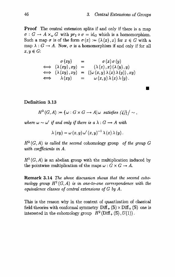
46 3. Central Extensions of Groups
P r o o f The central extension splits if and only if there is a map a : G ~ A ×~ G with pr2 o a = idG which is a homomorphism. Such a map a is of the form a ( x ) : = ()~ (x), x) for x E G with a map )~ : G ~ A. Now, a is a homomorphism if and only if for all x, y E G:
B
Def in i t ion 3.13
H 2 (G, A ) : = {w" G x G ~ AI w satisfies (~)}1 ,.~,
where w .,, w' if and only if there is a )~ " G ~ A with
H 2 (G, A) is called the second cohomology group
with coefficients in A. of the group G
H 2 (G, A) is an abelian group with the multiplication induced by the pointwise multiplication of the maps w" G x G ~ A.
R e m a r k 3.14 The above discussion shows that the second coho- mology group H 2 (G, A) is in one-to-one correspondence with the equivalence classes of central extensions of G by A.
This is the reason why in the context of quantization of classical field theories with conformal symmetry Diff+ (S) x Diff+ (S) one is interested in the cohomology group g 2 (Diff+ (S), V(1)).
4 Central Extensions of Lie Algebras and Bargmann's Theorem
In this section some basic results on Lie groups and Lie algebras are assumed to be known, as presented, for instance, in [HN91] or [BR77]. For example, every finite-dimensional Lie group G has a corresponding Lie algebra Lie G determined up to isomorphism, and every differentiable homomorphism R" G --, H of Lie groups induces a Lie-algebra homomorphism Lie R = / ~ " Lie G --, Lie H. Conversely, if H is connected and simply connected, every such Lie-algebra homomorphism p" Lie G --, Lie H determines a unique differentiable Lie-group homomorphism R" G --, H with/~ = p.
In addition, for the proof of Bargmann's theorem we need a more involved result due to Montgomory and Zippin, namely the solution of one of Hilbert's problems: every topological group G, which is a topological manifold (i.e. every x E G has an open neighborhood U with a topological map ~" U --, R~), is already a Lie group (cf. [MZ55])" G has a differentiable structure (i.e. it is a differentiable manifold), such that the composition (g, h) --, gh and the inversion g __, g-1 are differentiable mappings.
4.1 Central Extensions and Equivalence
A Lie algebra a is called abelian if the Lie bracket of a istrivial, i.e. IX, Y] = 0 for all X, Y E a.
Definition 4.1 Let a be an abelian Lie algebra over IK and g a Lie algebra over IK (the case of dim 9 = oc is not excluded). An exact sequence of Lie-algebra homomorphisms
0 )a ~0 ' ~ g ~0
is called a central extension of g by a, if [a, O] = O, i.e. IX, Y] = 0 for all X E a and Y E O. Here we identify a with the corresponding subalgebra of ~.
48 4. Central Extensions of Lie Algebras
E x a m p l e s :
• Let 1 >A / n ~E >G >1
be a central extension of finite-dimensional Lie groups A, E and G with differentiable homomorphisms I and R. Then, for i = Lie I and/~ = Lie R the sequence
J 0 > LieA >LieE > LieG >0
is a central extension of Lie algebras.
• In particular, every central extension E Of the Lie group G
by U(1)
1 >U(1) >E R>G >1
with a differentiable homomorphism R induces a central ex- tension
0 >IR > LieE > LieG >0
of the Lie algebra Lie G by the abelian Lie algebra R ~ iR LieU(l).
• The Virasoro algebra is the central extension of the Witt al- gebra (cf. Sect. 5).
Defini t ion 4.2 An exact sequence of Lie algebra homomorphisms
0 ~a >0 ~ g >0
splits if there is a Lie-algebra homomorphism /3 " g ~ l] with r o/3 = idg. The homomorphism fl is called a splitting map. A central extension which splits is called a trivial extension, since it is equivalent to the exact sequence of Lie-algebra homomorphisms
0 >a ~a@g ~g >0.
(Equivalence is defined in analogy to the group case, cf. the discus- sion after 3. 8.)
4.1 Central Extensions and Equivalence 49
If, in the preceding examples, the sequence of Lie groups splits in the sense of Sect. 3 (with a differentiable homomorphism S : G ---. E as splitting map), then the corresponding sequence of Lie- algebra homomorphisms also splits in the sense of Definition 4.2 with splitting map S. In general, the reverse implication holds for connected and simply connected Lie groups G only. In this case, the sequence of Lie groups splits if and only if the associated sequence of Lie algebras splits. All this follows immediately from the properties stated at the beginning of this section.
R e m a r k 4.3 For every central extension of Lie algebras
0 >a >~ 7r " ~ g > 0
there is a linear homomorphism ~ : g ~ [) with lr o ~ = idg. Let
o (x, Y) .= [9 (x) , Z (Y)] - Z (IX, Y]) for x, Y e g.
Then ~ is a splitting map if and only if 0 = O.
It can easily be checked that the map 0 : g × g --"* a (depending on /3) always has the following three properties:
1 o O: g × 9 ~ a is bilinear and alternating.
2 ° o (x, [Y, z]) + o (Y, [z, x]) + o (z, [x, Y]) = o.
3 ° ~ ~- g @ a as vector spaces by the linear isomorphism
¢ : g x . - . 0 , x e z = ( x . z ) ~ 9 ( x ) + z .
with the following Lie bracket
IX + z, y + z']0 = IX, Y], + o (x, Y)
for X , Y E g and Z, Z ~ E a. Emphasizing the dependence of this Lie bracket on ~ it also can be written as
[,6'(X) + Z,/3(Y) + Z'] =/3 ([X, Y]) + O (X, Y).
Here, we treat a as a subalgebra of 0 again.
50 4. Central Extensions of Lie Algebras
L e m m a 4.4 is as follows:
1. Every central extension ~ of g by a comes from a mapping O " g x g ---+ a with the properties 1° and 2 °.
2. Every O" g x g ~ a with the properties 1 ° and 2 ° a central extension I~ of g by a (according to 3°).
generates
3. Such a central extension splits (i.e. there is a # E HomK (g, a) with
is trivial) if and only if
O (X, Y) = # ([X, Y]).
P r o o f 1." is obvious from the preceding discussion. 2." Let 0 be the vector space b := g @ a. The bracket
[X @ Z, Y @ Z']~ "= [X, Y]g @ O(X, Y)
for X, Y E g and Z, Z' E a is a Lie bracket if and only if the map O satisfies 1 o and 2 o. Hence, ~ with this Lie bracket defines a central extension of g by a. 3.: Let a : g ---, I~ - g @ a a splitting map. Then a has to be of the form a ( X ) = Z + # ( Z ) , Z e g, with a suitable # E HomK (g, a). From the definition of the bracket on ll, [a(X), a(Y)] = [X, Y] + O(X, Y) for X, Y e g. Furthermore, since a is a Lie-algebra homomorphism, [a(X), a(Y)] = a([X, Y]) = [X, Y] + #([X, Y]). It follows that O (X, Y) = # ([X, Y]). Con- versely, if O has this form, it clearly satisfies 1 o and 2 °. The linear map a : g --+ ll = g @ a defined by a ( X ) : = X + #(X), X E g, turns out to be a Lie-algebra homomorphism:
o([x,z]) = [X, Y]g + # ([X, Y])
= [ X , Y ] g + e ( X , Y )
= [X + # (X) , Y + # (Y)]~
= [ a ( X ) , a ( Z ) ] ~ .
Hence, a is a splitting map. I
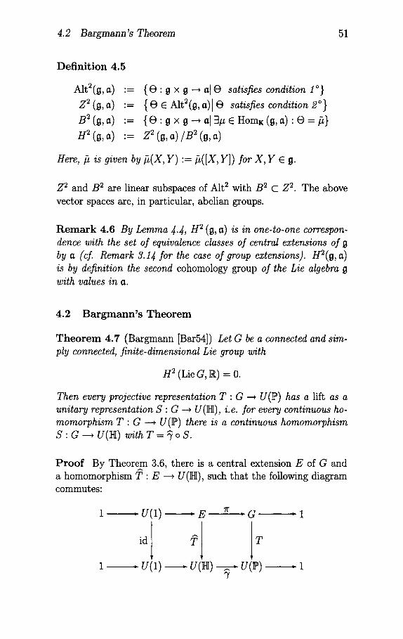
4.2 Bargmann 's Theorem 51
Def in i t i on 4.5
Alt2(g, a ) : = Z 2 (g, a) : =
B 2 (g, a) :=
H2 (it, a) :=
{ O ' g x g ~ a[ t3 satisfies condition 1°}
{ O e Alt2(g, a ) l e satisfies condition 2 ° }
{ e t t x tt --, a[ 3# e HomK (g, a)" O = t5}
z ~ ( g . . ) / B ~ (g. . )
Here, ~ ~ g~en by ~(x, Y) .= ~([x, Y])/o~ x, Y e g.
Z 2 and B 2 are linear subspaces of Alt 2 with B 2 C Z 2. The above vector spaces are, in particular, abelian groups.
R e m a r k 4.6 By Lemma 4.4, H2 (g, a) is in one-to-one correspon- dence with the set of equivalence classes of central extensions of g by a (cf. Remark 3.14 for the case of group extensions). U2(tt, a) is by definition the second cohomology group of the Lie algebra g with values in a.
4.2 Ba rgmann ' s Theorem
Theo rem 4.7 (Bargmann [Bar54]) Let G be a connected and sim- ply connected, finite-dimensional Lie group with
H 2 (Lie G, R) = 0.
Then every projective representation T : G ~ U(P) has a lift as a unitary representation S : G ~ U(]HI), i.e. for every continuous ho- momorphism T : G ---, U(IP) there is a continuous homomorphism S" G ---, U(H) with T = ~ o S.
Proo f By Theorem 3.6, there is a central extension E of G and a homomorphism T" E ~ U(]HI), such that the following diagram commutes"
1 ~U(1)
id 1
1 .U(1)
, E ~ , . G ;1
A
T T
u(~) ^, u(~) , 1
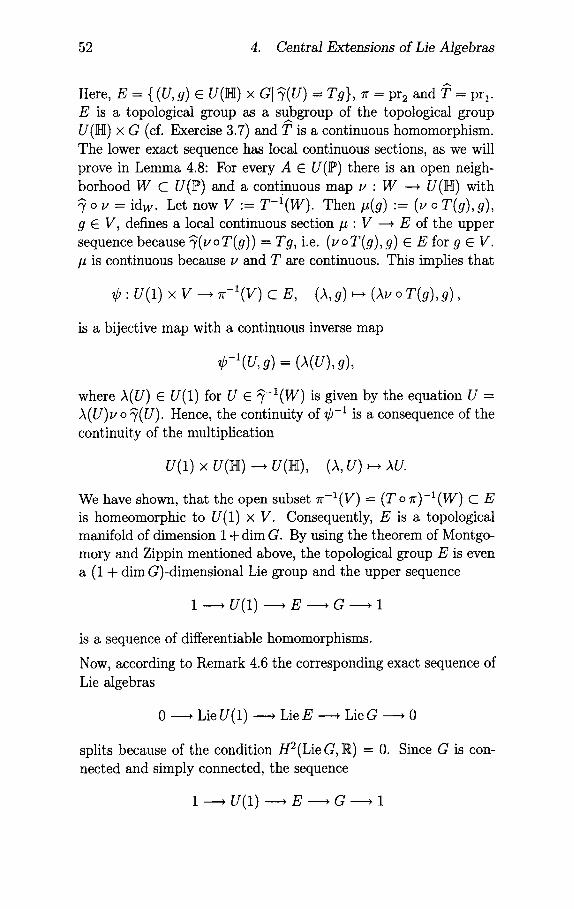
52 4. Central Extensions of Lie Algebras
A
Here, E = { (U, g) e U(]HI) x G[ ~(U) = Tg}, r = pr 2 and T = pr:. E is a topological group as a subgroup of the topological group U(]E) x G (cf. Exercise 3.7) and T is a continuous homomorphism. The lower exact sequence has local continuous sections, as we will prove in Lemma 4.8: For every A E U(P) there is an open neigh- borhood W C U(IP) and a continuous map u : W ---, U(H) with
o u = idw. Let now V "= T-i(W). Then # ( g ) : = (u o T(g), g), g E V, defines a local continuous section # : V ---, E of the upper sequence because ~(u o T(g))= Tg, i.e. (u o T(g), g) E E for g e V. # is continuous because u and T are continuous. This implies that
¢ " U(1) x V ---, r - l ( v ) C E, (A, g) ~ (Au o T(g), g),
is a bijective map with a continuous inverse map
~)-l(v~ g) = ()~(U), g),
where A(U) e U(1) for U e ~ - I (W) is given by the equation U = A(U)u o ~(U). Hence, the continuity of ¢-1 is a consequence of the continuity of the multiplication
U(1) x U(H)---, U(H), (A, U)~-, AU.
We have shown, that the open subset zr-:(V) = (T o 71)- l (W) C E is homeomorphic to U(1) x V. Consequently, E is a topological manifold of dimension 1 + dim G. By using the theorem of Montgo- mory and Zippin mentioned above, the topological group E is even a (1 + dim G)-dimensional Lie group and the upper sequence
1 > U(1) > E , G ,1
is a sequence of differentiable homomorphisms.
Now, according to Remark 4.6 the corresponding exact sequence of
Lie algebras
0 , Lie U(1) > Lie E > Lie G > 0
splits because of the condition H2(Lie G, R) = 0. Since G is con- nected and simply connected, the sequence
1 > U(1) ~ E ; G > 1
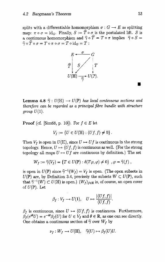
4.2 Bargmana 's Theorem 53
splits with a differentiable homomorphism a" G ---. E as splitting map: r o a = ida. Finally, S := T o a is the postulated lift. S is a continuous homomorphism and ~ o T = T o 1r implies 7 o S =
A A
7 o T o a = T oTr o a = T o i d a = T "
E-" a G
u(H) . . ,
7 I
L e m m a 4.8 ~ • U(IHI) ---. U(]P) has local continuous sections and therefore can be regarded as a principal fibre bundle with structure group U(1).
P r o o f (cf. [Sim68, p. 10]). For f e E let
Y$ "= {U e U(IHI)" (U f, f ) ¢ 0}.
Then VI is open in U(IHI), since U ~ U f is continuous in the strong topology. Hence, U ~ (U f , f ) is continuous as well. (For the strong topology all maps U ~ U f are continuous by definition.) The set
W I "= ~(VI) = {T e U(I?) • ~(T~, q0) ~ 0} , ~ = ~ ( f ) ,
is open in U(I?) s ince ~ - l ( W f ) -- Yf is open. (The open subsets in U(I?) are, by Definition 3.4, precisely the subsets W C U(IP), such that ~ - : ( W ) C U(]E) is open.) (Wi)fen is, of course, an open cover of U(I?). Let
j~f " V f - - "+ U(1), U I(Uf, f ) l
<Uf, f ) "
/31 is continuous, since U ~-~ (U f, f ) is continuous. Furthermore, ~f(eWU) = e-i°13l(U ) for U 6 VI and 0 E R, as one can see directly. One obtains a continuous section of ~ over W I by
. u ( s ) , Z (u)v.
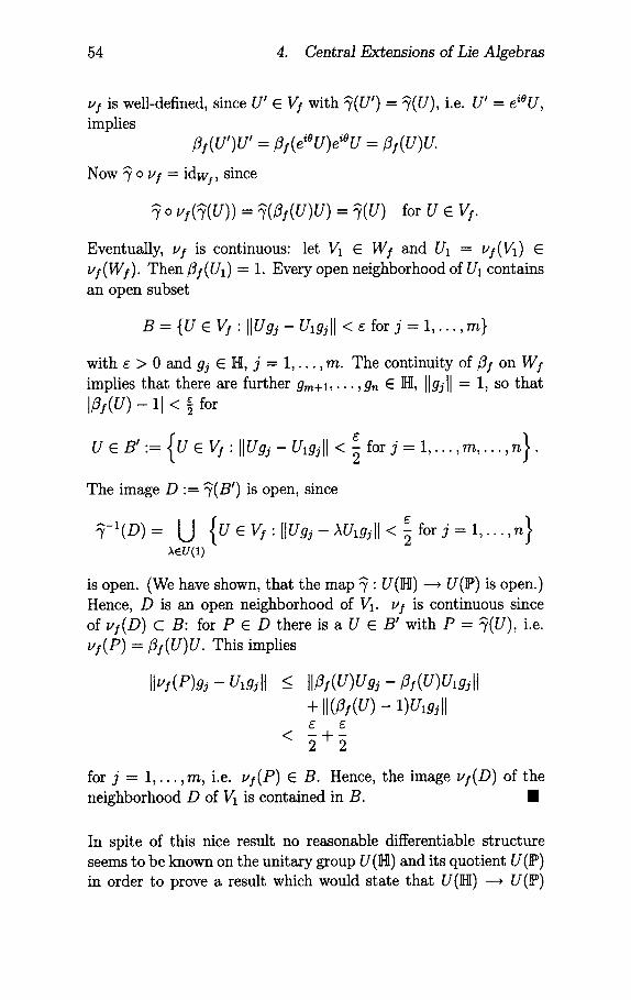
54 4. Central Extensions of Lie Algebras
yi is well-defined, since U' 6 V! with ~(U') = ~(U), i.e. U'= e~°U, implies
~ ( v ' ) v ' = ~ ( ¢ ° v ) ¢ ° v = ~ ( v ) u .
Now ~ o ~,f = idws, since
o vi(~(U)) = ~(~I(U)U) = ~(U) for U e V s.
Eventually, v I is continuous" let 1/1 E W I and U1 = vf(V1) E ~,I(WI). Then/3I(U1 ) = 1. Every open neighborhood of U1 contains an open subset
B = {U e V~ ' I IUg j - Ulgjll < ~ for j = 1 , . . . , m}
with ~ > 0 and g3 q IHI, j = 1 , . . . , m. The continuity of f~f on Wf implies that there are further gm+l, . . . ,gn E N, Jig/I[ = 1, so that [ f~s(U)- II < ~ for
U E B ' : = { U E V f • l lUgj- ulgjll < ~ for j = l,...,m,...,n}
The image D := ~(B') is open, since
^ - -y { ~ ~ ,n } l(D) = [.j V e Y~" llVgj-~Vlgjll < for j = 1 , . . . ~u(x)
is open. (We have shown, that the map ~" U(H) ---. U(IP) is open.) Hence, D is an open neighborhood of 1/1. v I is continuous since of vI(D ) C B" for P 6 D there is a U 6 B' with P = ~(U), i.e. vf(P) = $I(U)U. This implies
[[vl(P)gj - ulgjll < IIZ~(u)ugj - z~ (u )v ig j l l
+ I I@(U) - 1)Vlgjll 6 E
< ~ + ~
for j = 1 , . . . , m, i.e. vf(P) 6 B. Hence, the image vf(D) of the neighborhood D of V1 is contained in B. m
In spite of this nice result no reasonable differentiable structure seems to be known on the unitary group U(H) and its quotient U(IP) in order to prove a result which would state that U(H) ---, U(IP)
4.2 Bargmann 's Theorem 55
is a differentiable principal fibre bundle. The difficulty in defining a Lie-group structure on the unitary group lies in the fact that the corresponding Lie algebra should contain the (bounded and unbounded) self-adjoint operators on ]HI.
E is by construction the fibre product of ~ and T. Since ~ is locally trivial by Lemma 4.8 with general fibre U(1), this must also hold for E --, G. Exactly this was needed in the proof of Theorem 4.7, to show that E actually is a Lie group.
R e m a r k 4.9 For every finite-dimensional semi-simple Lie algebra g over IK one can show: H 2 (g, IK) = 0 (cf. [HN91]). As a con- sequence of the above discussion we thus have the following result which can be applied to the quantization of certain important sym- metries: if G is a connected and simply connected Lie group with simple Lie algebra Lie(G) = it, then every continuous represen- tation T • G --, U(IP) has a lift to a unitary representation. In particular, to every continuous representation T" SU(N) -~ U(~) (resp. T " SL(2, C) --+ U(IP)) there corresponds a unitary repre-
S. SU(N) U(H) # sp. S / ( 2 , C ) - , U(S)) th o S = T. Note, that SL(2, C) is the universal covering group of
the proper Lorentz group S0(3, 1).
5 T h e V i r a s o r o A l g e b r a
In this section we will describe how the Witt algebra and the Vi- rasoro algebra as its non-trivial central extension appear in the investigation of conformal symmetries.
5.1 Witt Algebra and Infinitesimal Conformal Transformations of the Minkowski Plane
The quantization of systems with symmetries yields representations of the classical symmetry group in U(P) (with I? - I? (H), the pro- jective space of a Hilbert space ]E, cf. Sect. 3), i.e. so-called projective representations. As we have explained in Sect. 2, the conformal group of R ~'~ is isomorphic to Diff+ (S) x Diff+ (S) (here and in the following S "= S 1 is the unit circle). Hence, given a the- ory with this conformal group as symmetry group, one studies the group Diff+ (S) and its Lie algebra first. After quantization one is interested in the unitary representations of the central extensions of Diff+ (S) or Lie (Diff+ (S)) in order to get representations in the Hilbert space as we have explained in the preceding two sections.
The group Diff+ (S) is in a canonical way an infinite-dimensional Lie group modeled on the real vector space of differentiable vector fields Vect (S). (We will discuss Vect (S) in more detail below.) Diff+ (S) is equipped with the topology of uniform convergence of the dif- ferentiable mappings ~ : S ~ S and all their derivatives. This topology is metrizable. Similarly, Vect (S) carries the topology of uniform convergence of the differentiable vector fields X :S ~ TS and all their derivatives. With this topology, Vect (S) is a Fr@chet space. In fact, Vect (S) is isomorphic to C°°(S, R), as we will see shortly. The proof that Diff+ (S) in this way actually becomes a differentiable manifold modeled on Vect (S) and that the group op- eration and the inversion are differentiable, is elementary and can be carried out for arbitrary-oriented, compact (finite-dimensional) manifolds M instead of S (cf. [Mi184]).
Since Diff+ (S) is a manifold modeled on the vector space Vect (S), every tangent space T~(Diff+ (S)) at a point ~ e Diff+ (S) is iso- morphic to the vector space Vect (S). Hence, Vect (S) also is the underlying vector space of the Lie algebra Lie(Diff+ (S)). A careful
5.1 The Witt Algebra and Minkowski Plane 57
investigation of the two Lie brackets on Vect (S) - one from Vect (S), the other from Lie(Diff+(S)) - shows, that each Lie bracket is ex- actly the negative of the other (cf. [Mil84]). However, this subtle fact is not important for the representation theory of Lie(Diff+ (S)). Consequently, it is usually ignored. So we set:
Lie(Diff+ (S)) := Vect (S).
The vector space Vect (S) i s - like the space Vect (M) of differ- entiable vector fields on a differentiable manifold M - an infinite- dimensional Lie algebra over R with a natural Lie bracket: a differ- entiable vector field X on M can be considered to be a derivation X'C°° (M) --. C°°(M), i.e. a R-linear map with
X(fg) = X(f)g + f X(g) for f, g e C~(M).
The Lie bracket of two vector fields X and Y is the commutator
IX, Y] := X o Y - Y o X
which turns out to be a derivation again. Hence, IX, Y] defines a differentiable vector field on M. For M = S the space C°°(S) can be described as the vector space C~(R) of 2r-periodic functions ]R ---, R. A general vector field X E Vect (S) in this setting has the form Z = f d , where f e C~(R) and where the points z of S are represented as z = e i°, 0 being a variable in R. For X = f d and y _ g d it is easy to see that
d g,= d f, d IX, Y] = ( f g ' - f'g)-~ with ~--~g and = f. (5)
The representation of f by a convergent Fourier series
o o
f (O) = ao + E ( a n cos(n0) + bn sin(n0)) n = l
leads to a natural (topological) generating system for Vect (S):
d d sin(n0) d d--O' cos(n0) ~-~, ~--~.
Of special interest is the complexification
Vect c (S)"= Vect(S)® C
58 5. The Virasoro Algebra
of Vect(S). To begin with, we discuss only the restricted Lie algebra W C Vect c (S) of polynomial vector fields on S. Define
Ln := z 1-n d ~ • -ino d d-z = - i z -" = -ze )-~ e Vect c (S),
for n e Z. Ln" C °~ (S, C) ~ C °~ (S, C), f ~ z l -" f '. The linear hull of the L, over C is called the Witt algebra"
W : = C { L . ' n E Z}.
It has to be shown, of course, that W with the Lie bracket in VectC(s) actually becomes a Lie algebra over C. For that, we de- termine the Lie bracket of the L,, Lm, which can also be deduced from the above formula (5). For n, m e N and f e C ~ (S, C)"
L.Lmf = z l - "d ( zl-'~d ) - ~ z -~z f
d 2 : (1 - m)zl-n-m£f -- z l - n z 1 - m f .
dz dz 2
This yields
[L,,Lm]f = L, L m f - LmL, f = ( ( 1 - m ) - ( 1 -
= ( n - m) L,+mf.
In a theory with conformal symmetry, the Witt algebra W is a part of the complexified Lie algebra Vect c (S) x Vect c (S) belonging to the classical conformal symmetry. Hence, as we mentioned in the preceding section, the central extensions of W by C become important for the quantization process.
5.2 Wit t Algebra and Infinitesimal Conformal Transformations of the Euclidean Plane
Before we focus on the central extensions of the Witt algebra in Theorem 5.1, another approach to the Witt algebra shall be de- scribed. This approach is connected with the discussion in Sect. 2.3 about the conformal group for the Euclidean plane. In fact, in the development of conformal field theory in the context of statisti- cal mechanics mostly the Euclidean signature is used. This point of
5.2 The Wit t Algebra and Euclidean Plane 59
view is taken, for example, in the fundamental papers on conformal field theory in two dimensions (cf. e.g. [BPZ84], [Gin89], [GO89]).
The conformal transformations in domains U C C ~ R 2'° are the holomorphic or anti-holomorphic functions with nowhere-vanishing derivative (cf. Theorem 1.11). We will treat only the holomorphic case for the beginning. If one ignores the question of how these holomorphic transformations can form a group (cf. Sect. 2.3), and investigates infinitesimal holomorphic transformations, these can be written as
z ~ z + y ~ an z n,
nEZ
with convergent Laurent series ~ e z an Z". In the sense of the gen- eral relation between Diff+(M) and Vect(M), the vector fields rep- resenting these infinitesimal transformations can be written as
~-~ anzn+l d dz
in the fictional relation between the "conformal group" and the vector fields. The Lie algebra of all these vector fields has the sequence (Ln)nez, Ln - z 1-nd, as a (topological) basis with the Lie bracket derived above:
[Ln, Lm] = (n - m)Ln+m.
Hence, for the Euclidean case there are also good reasons to intro- duce the Witt algebra W = C {Ln " n E Z} with this Lie bracket as the conformal symmetry algebra. The Witt algebra is a dense subal- gebra of the Lie algebra of holomorphic vector fields on C \ {0}. The same is true for an annulus {z E C ' r < Izl < R}, 0 < r < R < oo. However, only the vector fields L~ with 1 >_ n can be continued holomorphically to a neighborhood of 0 in C, the other L~'s are strictly singular at 0. As a consequence, contrary to what we have just stated the vector fields L~, n > 1, cannot be considered to be infinitesimal conformal transformations on a suitable neighborhood of 0. Instead, these meromorphic vector fields correspond to proper deformations of the standard conformal structure on R 2'° ~ C.
Without having to speak of a specific "conformal group" we can re- qu i r e - as it is usually done in conformal field theory ~ la [BPZ84]
60 5. The Virasoro Algebra
- that the primary field operators of a conformal field theory trans- form infinitesimally according to the L~. This symmetry condition yields an infinite number of constraints. This viewpoint explains the claim of "infinite dimensionality" in the citations of Sect. 2.3.
Let us point out that there is no complex Lie group H with Lie H = Vect c(s). This follows from a result of Herman [Her71].
The anti-holomorphic transformations/vector fields yield a copy W of W with basis L~, so that
[L~, Lm] = (n - m)L~+m and [L,, Lm] = 0.
For the Minkowski plane one has a copy of the Witt algebra as well, which in this case originates from the second factor Diff+ (S) in the characterization
Conf(R 1'1) ~ Diff+(S)x Diff+(S).
In both cases there is a natural isomorphism t : W ---, W of the Witt algebra, defined by t(L~) := -L_~ on the basis, t is a linear isomorphism and respects the Lie bracket:
[t(L,), t(Lm)l = [L_,, L_m] = - (n-m)L_( ,+m) = (n-m)t(L,+m).
Hence, t is a Lie-algebra isomorphism. Since t 2 = idw, t is an involution. These facts explain that in many texts on conformal field theory the basis
dz = t z 1-n
instead of L~ = z l - ~ is used. Incidentally, the involution t is 1 induced on W by the biholomorphic coordinate change z ~ w =
of the punctured plane C \ {0}: dz = -w-2dw implies
z l _ ~ d = w~_l(_w2) d _-_w~+ 1 d dz dw dw
5.3 The Viraso ro A lgeb ra as a C e n t r a l Extens ion of the Wit t Algeb ra
After these two approaches to the Witt algebra W we now come to the Virasoro algebra, which is a proper central extension of W. For existence and uniqueness we need
5.3 Central Extensions of the Witt Algebra 61
T h e o r e m 5.1 [GF68] H 2 (W, C) ~ C .
P r o o f In the following we show: the linear map w • W × W ~ C given by
3 n ( 1 for k = 0 w(n. ,nm):= . + m ] ~ ( n 2 - 1 ) , 3k:= 0 for k ¢ 0
defines a non-trivial central extension of W by C and up to equiv- alence this is the only non-trivial extension of W by C. In order to do this we prove
1. w c Z 2 ( W , C ) . 2. ~ ¢ B ~ (w, e l . 3. O E Z 2(W,C)=~3AEC'O, ,~AW.
Remark: the choice of the factor ~ in the definition of w is in accordance with the zeta function regulation using the Riemann zeta function, cf. [GSW87, p. 96].
1. Evidently, w is bilinear and alternating. In order to show w E Z 2 (W, C), i.e. 2 ° of Remark 4.3, we have to check that
w (Lk, [Lm, L.]) + w (Lm, [L., Lk]) + w (L., [Lk, Lm]) = 0
for k, m, n E Z. This can be calculated easily:
12(w (Lk, [Lm, L.]) + w (Lm, [L., L,I)
+w (L., [Lk, Lm]))
= 5k+rn+,.,((m- n)k (k 2 - 1) + ( n - k)m (m 2 - 1)
+ (k - m)n (n 2 - 1))
= - (m - n) (m + n) ( (m + n) 2 - 1 )
+ (2n + m)m (m ~ - 1)
- ( 2 m + n)n (n 2 - 1)
= 0
62 5. The Virasoro Algebra
2. Assume that there exists # E Homc (W, C) with w(X, Y) = #([X, Y]) for all X, Y E W. Then for every n E N we have
w (L~, L_.) = /5 (L., L_.)
=~ ~ ( n 2 - 1 ) = # ( [L . ,L_ . ] )
=~ ~ ( n 2 - 1) = 2n#(L0)
= l (n2 1 ) . =V # (L0) 2-X -
The last equation cannot hold for every n 6 N. So the as- sumption was wrong, which implies w ~ B 2 (W, C).
3. Let O E Z 2 (W, C). Then for k, m, n E Z we have
0 = e (Lk, [Lm, L.I) + e (Lm, [L., Lk]) + e (L., ILk, Lm])
= (m - n) 0 (Lk, Lm+.) + (n - k ) 0 (Lm, L.+k)
+ ( k - m ) O ( L . , L k + m ) .
For k = 0 we get
(m - n) O (L0, Lm+.) + nO (Lm, L.) - mO (L., Lm) = 0.
Hence
m ~ n O (L., Lm) = ~ O (Lo, L.~+.) for m, n e Z; m # - n .
m -f- n
We define a homomorphism # E Homc (W, C) by
# (Ln)._ _10 (Lo, L,) for n E Z \ {0}, n
1 #(Lo) "= --~O(L~, L_~ ),
and let O' "= O +/~. Then O' (L~, Lm) = 0 for m, n E Z, m - n , since
O'(L.,Lm) = O(L . ,Lm)+ #([L. ,Lm]) m m r t
m -f- n
m ~ n
m -4- n
- - 0 .
~ 0 (Lo, Ln+,n) + # ((n - m) L.+m)
n m m ~ 0 (Lo, Ln+m) + 0 (Lo, L.+m)
m + n
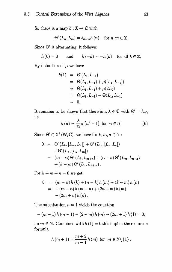
5.3 Central Extensions of the Witt Algebra 63
So there is a map h" Z --, C with
O' (L~, Lm) = 5n+mh (n) for n, m e Z.
Since O' is alternating, it follows"
h (0) = 0 and h ( - k ) - - h ( k ) for a l l k e Z .
By definition of # we have
h(1) = O'(L1, L- l )
---- O(L1, L-l) A- #([L1, L_~])
-- O(L1, L - l ) + #(2L0)
= O(L~, L_~) - O(L~, L- l )
0.
It remains to be shown that there is a A E C with O' = Aw, i.e.
A h ( n ) = ~ n (n 2 - 1) for n e N. (6)
Since O' E Z 2 (W, C), we have for k, m, n E N"
= O' (Lk, [Lm, L~]) + O' (Lm, [L~, Lk])
+O' (L~, [L~, Lm])
= (m - n) O' (Lk, Lm+~) + (n - k) O' (Lm, Ln+k) + (k - m) O' (Ln, Lk+m).
For k + m + n = 0 we get
O (m - n) h (k) + (n - k) h (m) + (k - m) h (n)
- (m - n) h (m + n) + (2n + m) h (m)
- (2m + n) h (n).
The substitution n = 1 yields the equation
- (m - 1) h (m + 1) + (2 + m) h (m) - (2m + 1) h (1) = 0,
for m E N. Combined with h (1) = 0 this implies the recursion formula
m + 2 h(m+ 1 ) =
m - - 1 ~ h ( m ) for m E N\{1} .
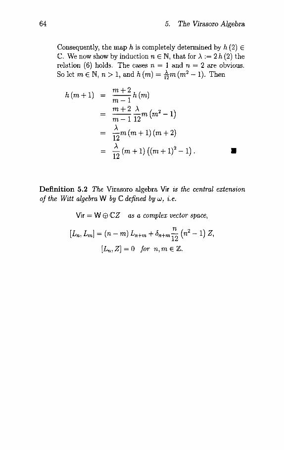
64 5. The Virasoro Algebra
Consequently, the map h is completely determined by h (2) E C. We now show by induction n E N, that for A := 2 h (2) the relation (6) holds. The cases n = 1 and n = 2 are obvious. So let m E N, n > 1, and h ( m ) - ~2 m (m 2 - 1). Then
m + 2
h ( m + l ) = ~ h ( m ) m - 1
_ m + 2 A - m - 1 12 m ( m 2 - 1 )
= -i-~m (m + 1 ) ( m + 2)
_ - A ( m + l ) ( ( m + l ) 2 12
1). I
Defini t ion 5.2 The Virasoro algebra Vir is the central extension of the Witt algebra W by C defined by w, i.e.
Vir = W @ C Z as a complex vector space,
n [Ln, Lm] = (n - m)L~+m + (in+,nT~ (n 2
[Ln, Z] =O for n, m E Z.
- 1) Z,
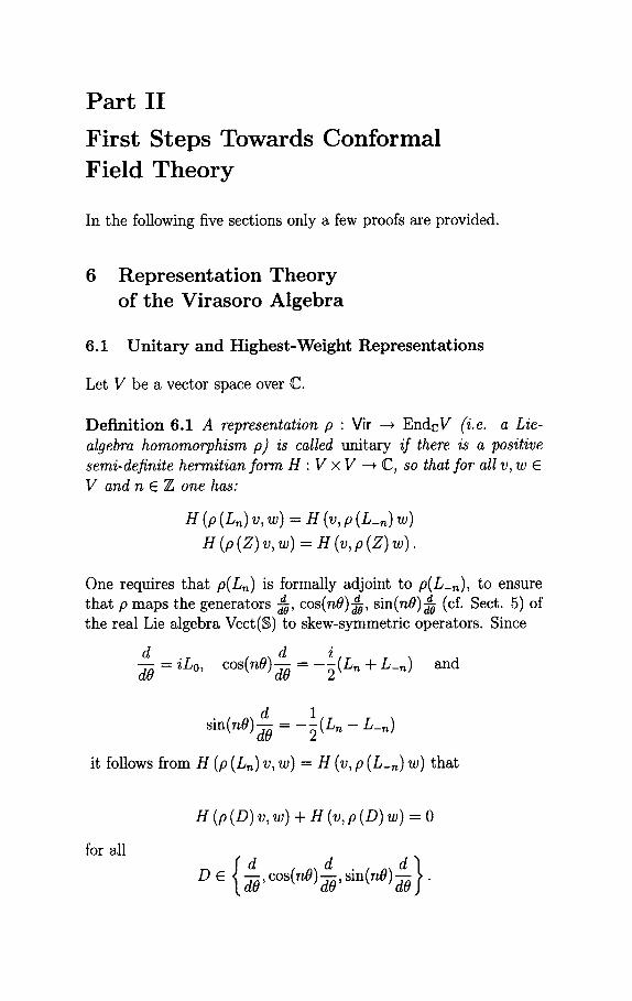
P a r t II
F i r s t S t e p s T o w a r d s C o n f o r m a l
F i e l d T h e o r y
In the following five sections only a few proofs are provided.
Representation Theory of the Virasoro Algebra
6.1 Unitary and Highest-Weight Representations
Let V be a vector space over C.
Defini t ion 6.1 A representation p " Vir --, EndcV (i.e. a Lie- algebra homomorphism p) is called unitary i f there is a positive semi-definite hermitian form H" V x V --, C, so that for all v, w E V and n E Z one has:
H (p (L.) v, w) = H (v, p (L_.)w)
H (p (Z)v, w) = H (v, p (Z)w).
One requires that p(Ln) is formally adjoint to p(L_n), to ensure that p maps the generators d , Cos(n0)d, sin(n0)~ (cf. Sect. 5) of the real Lie algebra Vect(S) to skew-symmetric operators. Since
d = iLo, cos(n0) d _ i (L n + L_n) and
d---0 d-0 - - 2
d sin(n0) ~--~ = I (L . - L_~)
2
it follows from H (p (L.)v, w) = H (v, p (L_.) w) that
for all
H (p (D) ~, ~) + H (v, p (D) ~) = 0
D e ~-~,cos(nO) ,sin(nO) .
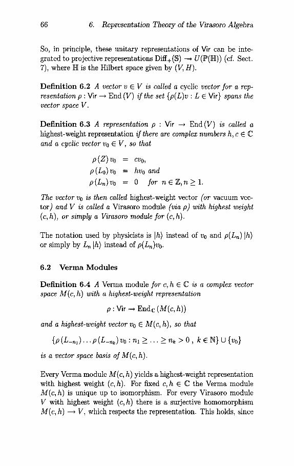
66 6. Representation Theory of the Virasoro Algebra
So, in principle, these unitary representations of Vir can be inte- grated to projective representations Diff+(S) --, U(P(]E)) (cf. Sect. 7), where ]HI is the Hilbert space given by (V, H).
Definition 6.2 A vector v E V is called a cyclic vector for a rep- resentation p" Vir --, End (V) / f the set {p ( i )v " L E Vir} spans the vector space V.
Definition 6.3 A representation p " Vir --, End(V) is called a highest-weight representation if there are complex numbers h, c E C and a cyclic vector Vo E V, so that
p ( Z) vo = CVo.
p ( Lo ) vo = hvo and
p(Ln)vo = 0 for n E Z, n > l.
The vector vo is then called highest-weight vector (or vacuum vec- tor) and V is called a Virasoro module (via p) with highest weight
h), a mod l h).
The notation used by physicists is I h) instead of v0 and p(Ln)I h) or simply by L~ ]h) instead of p(Ln)vo.
6.2 Verma Modules
Definition 6.4 A Verma module for c, h E C is a complex vector space M(c, h) with a highest-weight representation
p" Vir ~ Endc (M(c,h))
and a highest-weight vector Vo 6 M(c, h), so that
{p(L_,~). . .p(L_,k)v0 "nl >_... _ nk > 0, k E N} U {v0}
is a vector space basis of M(c, h).
Every Verma module M(c, h) yields a highest-weight representation with highest weight (c, h). For fixed c, h E C the Verma module M(c, h) is unique up to isomorphism. For every Virasoro module V with highest weight (c,h) there is a surjective homomorphism M(c, h) ~ V, which respects the representation. This holds, since
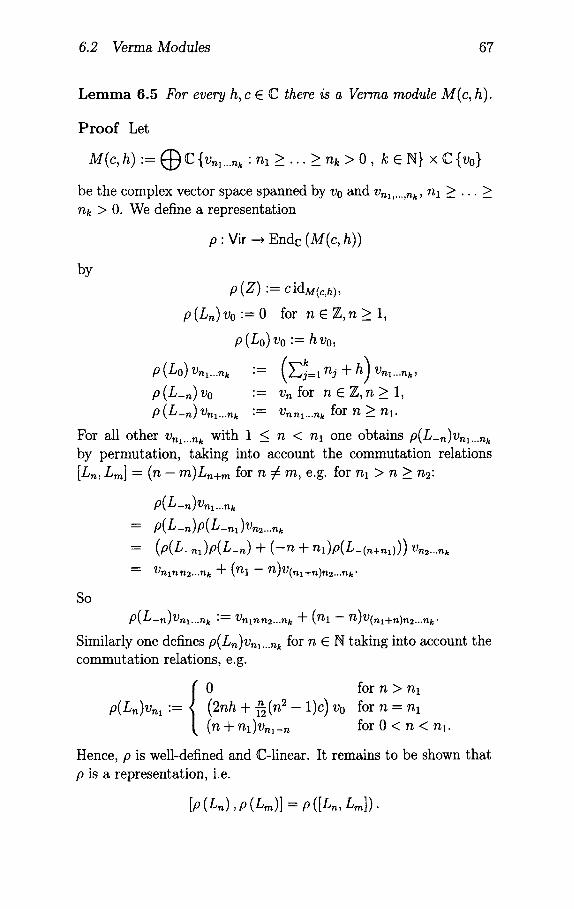
6.2 Verma Modules 67
L e m m a 6.5 For every h, c E C there is a Verma module M(c, h).
P r o o f Let
M(c, h ) := ( ~ C {v,1...n k "nl ~ . . . >_ nk > 0, k E N} x C {Vo}
be the complex vector space spanned by v0 and vn~,...,nk, nl k . . . k nk > 0. We define a representation
p" Vir --, Endc (M(c, h))
by
p (Z) "= c idM(c,h),
p(Ln) vo:=O for n E Z , n>__I,
p (Lo) Vo := h Vo,
p( io) Vnl...n k :-" (Ek=lIt j Jr-h)Vnl...nk, p(L_, )Vo := vn for n E Z ,n _> 1, p (L-n) v,~...nk := vnnl...nk for n _ nl .
For all other vni...nk with 1 _< n < nl one obtains p(L-,~)vn~...,k by permutation, taking into account the commutation relations [in, ira] : ( I t - r e ) i n + m for n # m, e.g. for n I > n _ n 2"
P(L-,)v,1...,k
= p(L_,)p(L_, , )v ,~. . . , k
= (p(n_n~)p(L_,) + ( - n + nl)p(L-(n+nl))) Vn2...nk
= v , ~ , ~ , ~ . . . , ~ + ( h i - n)v(,~+,~),~....,~.
So
p(L_n)v,,...,~ := vn,,n2...nk + (nl - n)v(n,+,)n2...,k.
Similarly one defines p( Ln )v,,..., k for n E N taking into account the commutation relations, e.g.
l 0 for n > n~
p(L~)v~, := (2nh + ~ ( n 2 - 1)c)Vo for n = nl
(n + nl)Vnl-n for 0 < n < nl.
Hence, p is well-defined and C-linear. It remains to be shown that p is a representation, i.e.
[p (L, ) , p (Lm)] = p ([L,, Lm]).
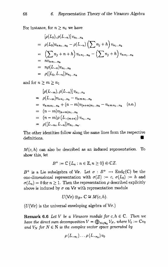
68 6. Representation Theory of the Virasoro Algebra
For instance, for n >_ n l we have
[p(Lo),p(L-,)]v,1...~k
--- p(io)Vnnl....k - p ( i_n ) (~ '~ nj + h)vnl...nk
= (~-~ nj + n + h)Vnn l . . . nk - ( E nj , h ) v n
-- TtVn nl...nk
= up(L_n)Vn 1...n k
= p([L0, L-~])v~...~k
n l . . . n k
and for n >_ m >_ n l
[p(L-m),p(L-~)lV~l...nk
= p(L_m)vn nl...nk -- Vn m n,...nk
= Vnmnx...n~ + (n -- m)v(n+m)n~...nk
= ( n - m)v(,~+,~)nl...nk
= (n - m)p (L-(m+n)) Vni...nk
= p([L-m,L-n])Vnl...nk.
Vn m nl...nk s.o.)
The other identities follow along the same lines from the respective
definitions, m
M(c,h) can also be described as an induced representation. To
show this, let
B + : = C { L n ' n E Z , n>__O}@CZ.
B + is a Lie subalgebra of Vir. Let a • B + --, Endc(C) be the one-dimensional representation with a ( Z ) " = c, a(Lo) := h and a(Ln) = 0 for n _> 1. Then the representation p described explicitly
above is induced by a on Vir with representation module
U(Vir) ®S+ C -~ M(c, h).
(U(Vir) is the universal enveloping algebra of Vir.)
R e m a r k 6.6 Let V be a Virasoro module for c, h 6 C. Then we have the direct sum decomposition V = (~NeNo VN, where Vo "= Cvo and VN for N 6 N is the complex vector space generated by
p (L_ , , ) . . . p (L_ ,k )Vo
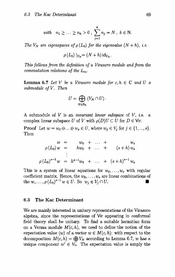
6.3 The Kac Determinant 69
k
with n~ > . . . > nk > O , y ] ~ n j = N , k E N . j=l
The V N are eigenspaces of p(Lo) for the eigenvalue ( g + h), i.e.
p (Lo)[vN = (N + h)idvN.
This follows from the definition of a Virasoro module and from the commutation relations of the Lm.
L e m m a 6.7 Let V be a Virasoro module for c, h E C and U a submodule of V. Then
u = G n u ) NENo
A submodule of V is an invariant linear subspace of V, i.e. a complex linear subspace U of V with p(D)U C U for D E Vir.
P r o o f Let w = wo @ ... @ w, E U, where wj E Vj for j E {1, ..., s}. Then
w - Wo + . . . + ws p (Lo) w = hwo + . . . + (s + h) w~
p (Lo)~-l w = h~-lWo + . . . + (s + h) ' - lw~
This is a system of linear equations for Wo,..., w~ with regular coefficient matrix. Hence, the w0, . . . , w~ are linear combinations of the w , . . . , p (Lo) "-1 w E U. So wj E Vj M U. I
6.3 T h e Kac D e t e r m i n a n t
We are mainly interested in unitary representations of the Virasoro algebra, since the representations of Vir appearing in conformal field theory shall be unitary. To find a suitable hermitian form on a Verma module M(c, h), we need to define the notion of the expectation value (w / of a vector w E M(c, h): with respect to the decomposition M(c, h) = ~)VN according to Lemma 6.7, w has a unique component w' E Vo. The expectation value is simply the
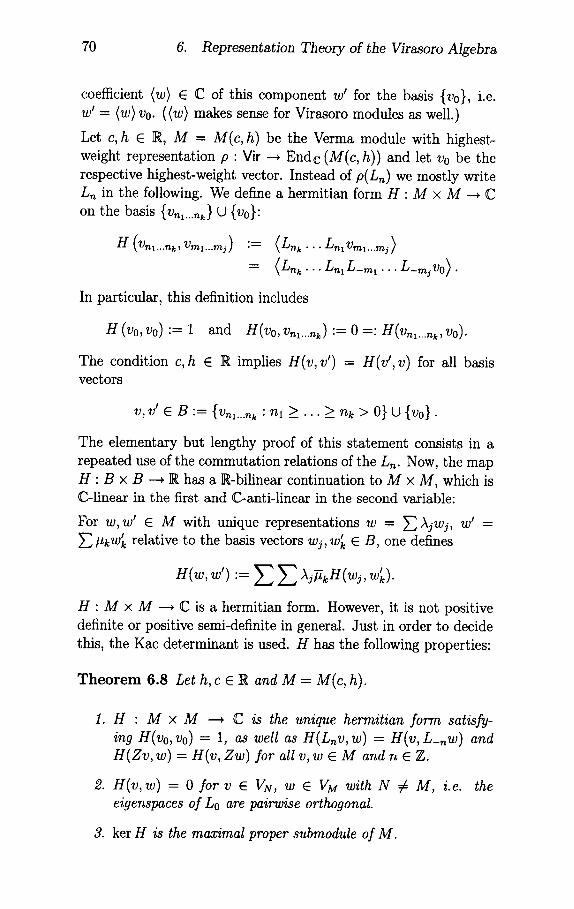
70 6. Representation Theory of the Virasoro Algebra
coefficient (w) E C of this component w' for the basis {v0}, i.e. w ' = (w)v0. ((w) makes sense for Virasoro modules as well.)
Let c, h E R, M = M(c,h) be the Verma module with highest- weight representation p" Vir ~ nndc ( i ( c , h ) ) and let Vo be the respective highest-weight vector. Instead of p(Ln) we mostly write Ln in the following. We define a hermitian form H" M x M -~ C on the basis {Vnl...nk} U {Vo}"
n ( v n l . . . n k , V m l . . . m j ) : - - ( L n k . . . L n l V m l . . . m j )
= L_ vo> In particular, this definition includes
H (v0, v0) "= 1 and H(vo, Vnl...nk ) :---- 0 = " H(vn~...nk, Vo).
The condition c,h E R implies H(v, v') = H(v', v) for all basis vectors
V, V t E B "= {Vnl...n ~ " n I ) _ . . . )__ it k > 0} U {Vo}.
The elementary but lengthy proof of this statement consists in a repeated use of the commutation relations of the Ln. Now, the map
H : B x B --~ R has a R-bilinear continuation to M x M, which is C-linear in the first and C-anti-linear in the second variable:
For w, w ~ E M with unique representations w = ~']~Ajwj, w ~ = #kw~k relative to the basis vectors wj, w~ E B, one defines
Z H : M × M --~ C is a hermitian form. However, it is not positive definite or positive semi-definite in general. Just in order to decide this, the Kac determinant is used. H has the following properties:
T h e o r e m 6.8 Let h, c E R and M = M(c, h).
1. H • M x M --, C is the unique hermitian form satisfy- ing H(vo, Vo) = 1, as well as H( inv , w) = H(v ,L_nw) and H(Zv , w) = H(v, Zw) for all v, w E M and n E Z.
2. H(v ,w) = 0 for v E VN, w E VM with N ~ M, i.e. eigenspaces of Lo are pairwise orthogonal.
the
3. ker H is the maximal proper submodule of M.
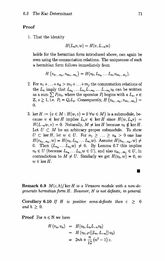
6.3 The Kac Determinant 71
P r o o f
1. That the identity
H(Lnv, w) = H(v, L_,w)
holds for the hermitian form introduced above, can again be seen using the commutation relations. The uniqueness of such a hermitian form follows immediately from
H (Vn~...nk, V,m...mj) = H(Vo, Lnk. . . Ln~ Vm~...mj ).
2. For nl -[-... +nk > ml -[-... + m j the commutation relations of the Ln imply that Lnk. . . Ln~L-m~... L-mjvo can be written as a sum ~ Plv0, where the operator Pt begins with a Ls, s E Z, s >_ 1, i.e. Pl = Qti~. Consequently, H (vn~...~k, vm~...mj) = 0.
3. ker H "= {v e M" H(w, v) = 0 Vw e M} is a submodule, be- cause v E ke rH implies Lnv E kerH since H(w, Lnv) = H(L_nw, v) = O. Naturally, M ~ ker H because v0 ~ ker g . Let U C M be an arbitrary proper submodule. To show U C kerH, let w E U. For n l _ . . . >__ nk > 0 one has H(vn~...nk, w) = g(vo, n~k . . . Ln, w). Assume H(vn~...nk, w) 0. Then (L~k... Ln~w) ~ O. By Lernma 6.7 this implies Vo E U (because Lnk.. . Ln~w E U), and also vm~...m~ E U, in contradiction to M ~ U. Similarly we get H(vo, w) = 0, so w E ker H.
m
R e m a r k 6.9 M(c, h) /ker H is a Virasoro module with a non-de- generate hermitian form H. However, H is not definite, in general.
C o r o l l a r y 6.10 If H is positive semi-definite then c and h > O.
> 0
P r o o f For n E N we have
H(v~,v~) = H(vo, LnL_~vo)
= H (vo, p ([L~, L-n]) vo) n
= 2 n h + ~ ( n 2 - 1 ) c.
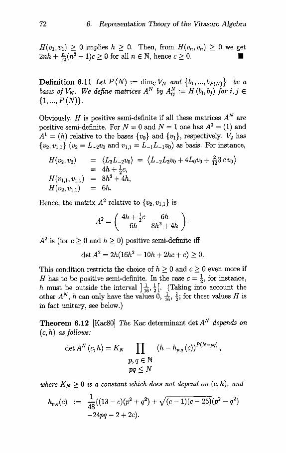
72 6. Representation Theory of the Virasoro Algebra
H(vx,vl) >_ 0 implies h _ 0. Then, from H(vn, vn) >_ 0 we get 2nh + ~ ( n 2 - 1)c __ 0 for all n E N, hence c ___ 0. I
De f in i t i on 6.11 Let P ( N ) ' = dimc VN and {bl,.. . ,bp(g)} be a basis of VN. We define matrices A N by A~ g := H (b~, b3) for i, j E {1, ..., P (N)}.
Obviously, H is positive semi-definite if all these matrices A N are positive semi-definite. For N = 0 and N = 1 one has A ° = (1) and A I = (h)relat ive to the bases {vo} and {Vl}, respectively. V2 has {V2, Vl,1} ( V 2 - L-2vo and Vl, 1 -- L-1L-lVo) as basis. For instance,
H(v2,v2)
H(Vl,l, Vl,1) U(v2, Vl,1)
Hence, the matrix A 2 relative to {v2, vl,1} is
1 6h A2 = 4h + ~c 6h 8h 2 + 4h
= <L2L-2vo) = (L-2L2vo + 4Lovo + ~3cvo> 4h + ½c,
= 8h 2 + 4h, = 6h.
.
A 2 is (for c >__ 0 and h >_ 0) positive semi-definite iff
det A 2 = 2h(16h 2 - 10h + 2hc + c) >__ O.
This condition restricts the choice of h > 0 and c > 0 even more if 1 for instance, H has to be positive semi-definite. In the case c - - ~,
1 h must be outside the interval ] ~ , ~ [. (Taking into account the 1 other A N h can only have the values 0, ~ , ~; for these values H is
in fact unitary, see below.)
T h e o r e m 6.12 [Kac80] The Kac determinant de tA g depends on (c, h) as follows:
det A N (c, h) = KN I I
p, q E N pq<_ N
(h - hp,q (c)) P(N-pq)
where KN >_ 0 is a constant which does not depend on (c, h), and
1 q2 hp,q(C) "= 4---~((13 - c)(p 2 + ) + V / ( c - 1 ) ( c - 25)(p 2 - q2)
- 2 4 p q - 2 + 2c).
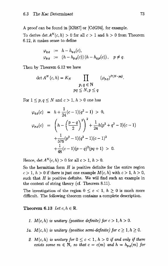
6.3 The Kac Determinant 73
A proof can be found in [KR87] or [CdG94], for example.
To derive det A N(c, h) > 0 for all c > 1 and h > 0 from Theorem 6.12, it makes sense to define
~q,q "-- h - hq,q (c) ,
~,,q "= ( h - hp,q(C)) ( h - hq,,(c)), p ~ q.
Then by Theorem 6.12 we have
det A N (c, h) = KN I I
p, q E N pq<_N,p<_q
(~p ,q)P(N-pq)
For 1 _< p,q <_ N and c > 1, h > 0 one has
h + 1 ( c - 1)(q 2 - 1) > 0,
P - q 2 + l h(p2 + q2 - 2
1 +g~__~(p2 _ 1)(q2 _ 1 ) ( c - 1) 2
1 (c - 1 ) ( p - q)2(pq ÷ 1) > 0.
Hence, det A N (c, h) > 0 for all c > 1, h > 0.
So the hermitian form H is positive definite for the entire region c > 1, h > 0 if there is just one example M(c, h) with c > 1, h > 0, such that H is positive definite. We will find such an example in the context of string theory (cf. Theorem 8.11).
The investigation of the region 0 <_ c < 1, h >_ 0 is much more difficult. The following theorem contains a complete description.
T h e o r e m 6.13 Let c, h E R.
I. M(c, h) is unitary (positive definite) for c > 1, h > O.
la. M(c, h) is unitary (positive semi-definite) for c >_ 1, h >_ O.
2. M(c, h) is unitary for 0 ~ c < 1, h > 0 if and only if there exists some m e N, so that c = c(m) and h = hp,q(m) for
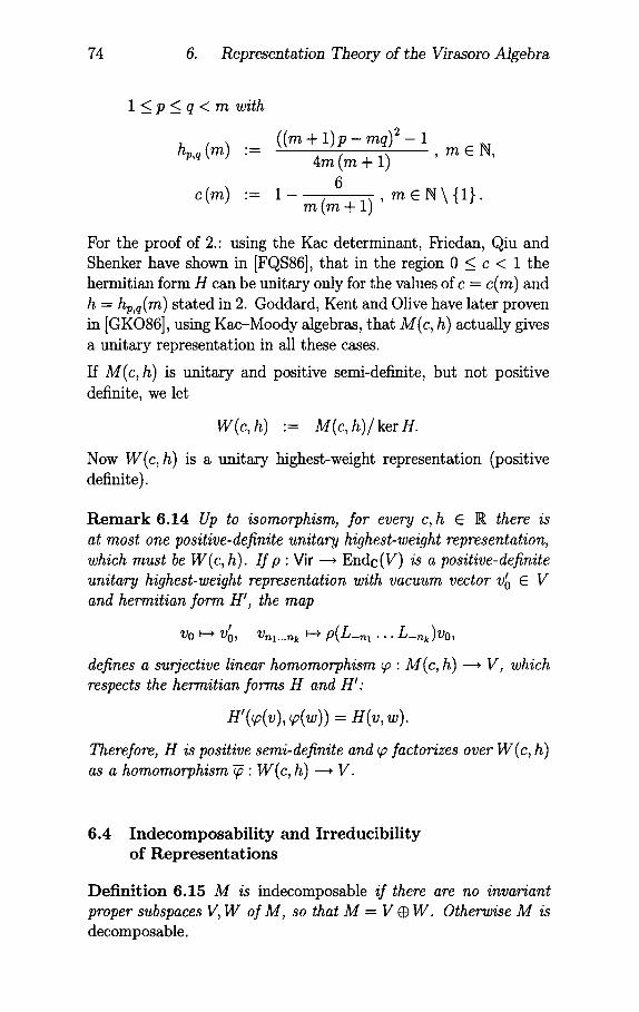
74 6. Representation Theory of the Virasoro Algebra
1 <_ p <_ q < m with
((m + 1 ) p - mq) 2 - 1 hp,q (m)
= 4m(m + 1) , m E N ,
6 c(m) "= 1 - m E N \ { 1 } .
m ( m + 1) '
For the proof of 2." using the Kac determinant, Friedan, Qiu and Shenker have shown in [FQS86], that in the region 0 _< c < 1 the hermitian form H can be unitary only for the values of c = c(m) and h = hp ,q (m) stated in 2. Goddard, Kent and Olive have later proven in [GKO86], using Kac-Moody algebras, that i ( c , h) actually gives a unitary representation in all these cases.
If M(c, h) is unitary and positive semi-definite, but not positive definite, we let
W(c, h) "= M(c, h)/ ker H.
Now W(c, h) is a unitary highest-weight representation (positive definite).
R e m a r k 6.14 Up to isomorphism, for every c,h E IR there is at most one positive-definite unitary highest-weight representation, which must be W(c, h). If p: Vir --+ nndc(V) is a positive-definite unitary highest-weight representation with vacuum vector v' o E V and hermitian form H', the map
!
Vo ~ v o, Vn~...nk ~ P(L-m .. . L-nk)Vo,
defines a surjective linear homomorphism ~o " M(c, h) --+ V, which respects the hermitian forms H and H"
H'(~(v), ~(w)) = H(v, w).
Therefore, H is positive semi-definite and ~ factorizes over W(c, h) as a homomorphism-~" W(c, h) ~ V.
6.4 Indecomposability and Irreducibility of Representations
Definition 6.15 M is indecomposable if there are no invariant proper subspaces V, W of M, so that M = V @ W. Otherwise M is decomposable.
6.4 Indecomposability and Irreducibility of Representations 75
Definition 6.16 M is called irreducible if there is no invariant proper subspace V of M. Otherwise M is called reducible.
T h e o r e m 6.17 For each weight (c, h) we have the following.
1. The Verma module M(c, h) is indecomposable.
2. If M(c,h) is reducible, then there is a maximal invariant subspace I (c, h), so that M(c, h)/ I (c, h) is an irreducible highest-weight representation.
3. Any positive-definite unitary highest-weight representation (i.e. W(c,h), see above) is irreducible.
P r o o f
1. Let V, W be invariant subspaces of M = M(c, h), and M = V @ W. By Remark 6.7, we have the direct sum decomposi-
tions
V = ¢ (Mj N V) and W = ( ~ (Mj A W) .
Since dim Mo = 1, this implies (Mo n V) = 0 or (M0 n W) = 0. So the highest-weight vector vo is contained either in V or in W. From the invariance of V and W it follows, that V = M o r W = M .
2. Let I(c, h) be the sum of the invariant proper subspaces of M. Then I(c, h) is an invariant proper subspace of M and i ( c , h ) / I ( c , h ) is an irreducible highest-weight representa- tion.
3. Let V be a positive-definite unitary highest-weight represen- tation and U c V be an invariant subspace. Then
U±= {v E V" H(u ,v )= OVa E U}
is an invariant subspace as well, since
U(u, L,v) = U(L_,u, v) = 0
and U @ U ± = V. So 3. follows from 1.
I
Projective Representations of Diff+ (S) and More
We know the unitary representations p~,h " Vir ~ End (W~,h) for c _> 1, h _ 0 or c = c(m), h = hp,q (m) from the discrete series, where W~,h := W(c, h) is the unique unitary highest-weight repre- sentation of the Virarsoro algebra Vir described in the preceding section. Let IE := W~,h be the completion of W~,h with respect to its Hermitean form. It can be shown that there is a linear subspace W~,h C ]HI, W~,h C W~,h, so that P~,h (~) has a linear continuation
P~,h (~) on W~,h for all ~ E Vir N (Vect(S)), where P~,h (~) is an es- sentially self-adjoint operator. The representation Pc,h is integrable in the following sense:
T h e o r e m 7.1 [GW85] There is a projective unitary representation Uc,h" Diff+ (S) ~ U (?(]E)), so that
(exp (-fic,h (~))) = U~,h (exp(~))
for all ~ E Vect(S), i.e. for all real vector fields ~ in S. Furthermore, for X e Vect(S)® C and ~ e Diff+(S) one has
U~,h(~)p¢,h(X) = (p¢,h(T~X) + ca(X, ~)) U¢,h(~)
with a map a on Vect(S) x Diff+(S). Here, the U~,h(~) are suitable lifts to IE of the original U~,h(~) (cf. Sect. 3).
Further investigations in the setting of conformal field theory lead to representations of
• "chiral" algebras A x A with Vir C A, Vir c A (here Vir is an isomorphic copy of Vir and ,4 as well as ,4 are further algebras), e.g. A = U (~) (universal enveloping algebra of a Kac-Moody algebra), but also algebras, which are neither Lie algebras nor enveloping algebras of Lie algebras. (cf. e.g. [BPZ84], [MS89], [FFK89], [Gin89], [GO89].)
• Semi-groups $ x ~ with Diff+(S) C $, Diff+(S) C $. One discusses semi-group extensions Diff+ (S), because there is no complex Lie group with Vect c (S) as the associated Lie algebra (cf. [Her71]).
7. Projective Representations of Diff+ (S) and More 77
We just present a first example of such a semi-group here (for a survey cf. [Gaw89])"
Example 7.2 Let q E C, T E C, q = exp(2riT), [q[ < 1 and Eq = {z e C[ [q[ <_ [z[_ 1} be the closed annulus with outer ra- dius 1 and inner radius [q[. Let gl, g2 e Diff+(S) be real analytic diffeomorphisms on the circle S. Then one gets the following pa- rameterizations of the boundary curves of Eq :
Pl (eiO) "--q gl (eiO),
The mentioned semi-group $ is the quotient of $o, where $o is the set of pairs (E,.p ~) of Riemann surfaces E with exactly two boundary curves parameterized by p' = (p~,p~), for which there is a q E C and a biholomorphic map ~ " Eq ~ E (where Pl,P2 is a para- meterization of OEq as above), so that ~ o pj = p~. As a set one has $ = $o/'~, where ,,~ means biholomorphic equivalence preserv- ing the parameterization. The product of two equivalence classes [(r~,p')], [(r:,p")] e $ is d¢~ned by "gluing" r~ and r:, where we identify the outer boundary curve of E with the inner boundary curve of E t taking into account the parameterizations.
The ansatz
A~,h ([Eq, p]) "= const U~,h (g21) q exp (P~,h (Lo)) U~,h (gl)
leads to a projective representation of E using Theorem 7.1.
More general semi-groups can be obtained by looking at more gen- eral Riemann surfaces, i.e. compact Riemann surfaces with finitely many boundary curves, which are parameterized and divided into incoming ("in") and outgoing ("out") boundary curves. The semi- groups defined in this manner have unitary representations as well (cf. [Seg91], [Seg88b] and [GW85]). Starting with these results, Segal has tried to give a useful definition of conformal field theory (cf. [SegS8a]).
8 String Theory as a Conformal Field Theory
In bosonic string theory as a classical field theory we have the flat semi-Riemannian manifold
(R D, 77) with ~ = diag ( -1 , 1, ..., 1)
as background space and a world sheet in this space, i.e. parameterization
x . Q - , R D
a C °°-
of a surface W = x (Q) C R D, where Q c R 2 is an open or closed rectangle. This corresponds to the idea of a one-dimensional object, the string, which moves in the space R D and wipes out the two- dimensional surface W = x (Q). The classical fields (i.e. the kinetic variables of the theory) are the components x" : Q ~ ]R of the parameterization x = ( x ° , x l , . . . , x D - 1 ) " Q ~ ~D of the surface
w = • (Q) c R
8.1 Ac t ion Func t iona l s and E q u a t i o n s of M o t i o n for St r ings
In classical string theory the admissible parameterizations, i.e. the dynamic variables of the world sheet are those, for which a given action functional is stationary. As a natural action of the classical field theory one uses the "area" of the world sheet in order to define the so-called Nambu-Goto action:
SNG (X) := --Pl; ~Q ~//-- det g dq°dq 1,
with a constant a E IR (the "string tension", cf. [GSW87]). Here, g "= x*~, (x*~),,~ = ~,jO, x~O~x j, is the metric on Q induced by x" Q ---, R D and the variation is taken only over those parameter- izations x, for which g is a Lorentz metric (at least in the interior of Q), i.e.
de t (g~) < 0.
Hence, (Q,g) is a two-dimensional Lorentz manifold, i.e. a two- dimensional semi-Riemannian manifold with a Lorentz metric g.
From the action principle
d d--~ SNG (X q- ~Y) le=o = 0
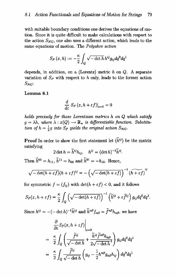
8.1 Action Functionals and Equations of Motion for Strings 79
with suitable boundary conditions one derives the equations of motion. Since it is quite difficult to make calculations with respect tothe action SNG, one also uses a different action, which leads to thesame equations of motion. The Polyakov action
K, f .. 0 1Sp(x,h):= -"2 lQ v-dethh'Jgiidq dq
depends, in addition, on a (Lorentz) metric h on Q. A separatevariation of Sp with respect to h only, leads to the former actionSNG:
Lemma 8.1
dde Sp (x, h + ef)le=o = 0
holds precisely for those Lorentzian metrics h on Q which satisfy9 = Ah, where A : x(Q) ~ lR+ is differentiable function. Substitution of h = :19 into Sp yields the original action SNG·
Proof In order to show the first statement let (hii ) be the matrixsatisfying
Then hOo = h11 , h11 = hoo and hOI = -h10 • Hence,
for symmetric I = (Iii) with det(h + c:1) < 0, and it follows
Sp(x, h + ef) = ~k(J- det(h +ef)) -1 (h,ii +efi ) giidqOdql.
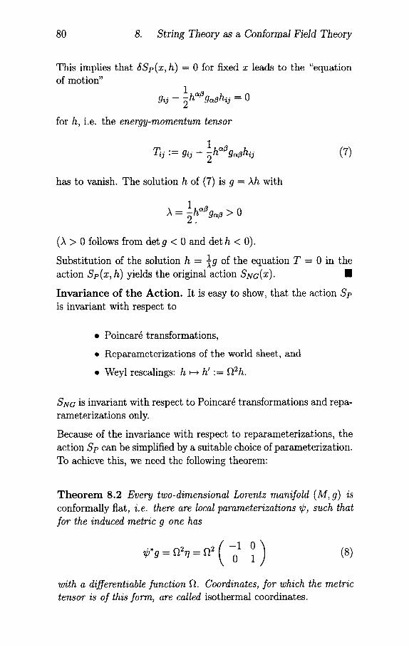
80 8. String Theory as a Conformal Field Theory
This implies that 5Sp(x, h) = 0 for fixed x leads to the "equation of motion"
1 g~j - -~ h ~ g~h~j = 0
for h, i.e. the energy-momentum tensor
1 T~j := g~j - -~ h ~g"~h~j (7)
has to vanish. The solution h of (7) is g = )~h with
= > 0
(£ > 0 follows from det g < 0 and det h < 0).
Substitution of the solution h = ½g of the equation T = 0 in the action Sp(x, h) yields the original action SNo(X). m
Inva r i ance of t he Act ion . It is easy to show, that the action Sp is invariant with respect to
• Poincar@ transformations,
• Repaxameterizations of the world sheet, and
• Weyl rescalings: h ~ h' := gt2h.
SNV is invariant with respect to Poincar@ transformations and repa- rameterizations only.
Because of the invariance with respect to reparameterizations, the action Sp can be simplified by a suitable choice of parameterization. To achieve this, we need the following theorem:
T h e o r e m 8.2 Every two-dimensional Lorentz manifold (M, g) is conformally flat, i.e. there are local parameterizations ¢, such that for the induced metric g one has
¢,g = f~2rl = ~2 ( - 1 0 \
o) 1 (8)
with a differentiable function ~. Coordinates, for which the metric tensor is of this form, are called isothermal coordinates.
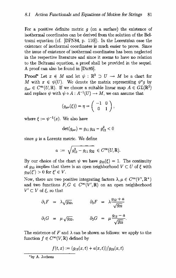
8.1 Action Functionals and Equations of Motion for Strings 81
For a positive definite metric g (on a surface) the existence of isothermal coordinates can be derived from the solution of the Bel- trami equation (cf. [DFN84, p. 110]). In the Lorentzian case the existence of isothermal coordinates is much easier to prove. Since the issue of existence of isothermal coordinates has been neglected in the respective literature and since it seems to have no relation to the Beltrami equation, a proof shall be provided in the sequel. A proof can also be found in [Dic89].
P r o o f Let x E M and let ¢ : R 2 D U ~ M be a c h a r t for
M with x E ¢(U). We denote the matrix representing ¢*g by g.~ e C°°(U, R). If we choose a suitable linear map A e GL(R 2) and replace ¢ with ¢ o A" A -1 (U) ~ M, we can assume that
- 1 (g"~(~)) = ~ = 0
0 1/ where ~ ' = ¢ - 1 ( x ) . We also have
det(g,~) = gll g22 - g~2 < 0
since g is a Lorentz metric. We define
/ a := ~/g122 -- g11g22 E C°°(U~).
By our choice of the chart ¢ we have g22(() = 1. The continuity of g22 implies that there is an open neighborhood V C U of ( with g22(~') > 0 for ~' e Y.
Now, there are two positive integrating factors ,~,# E C~(V~,R +) and two functions F, G E C°°(V',R) on an open neighborhood V ~ C V of ~, so that
01F = )~v/-~, 02F = ~g12 + a
g12 -- a 0 1 G = =
The existence of F and A can be shown as follows: we apply to the
function f E C°°(V, R) defined by
f (t, x) := (g12(x, t) + a(x, t))/g22(x, t)
*by A. J ochens
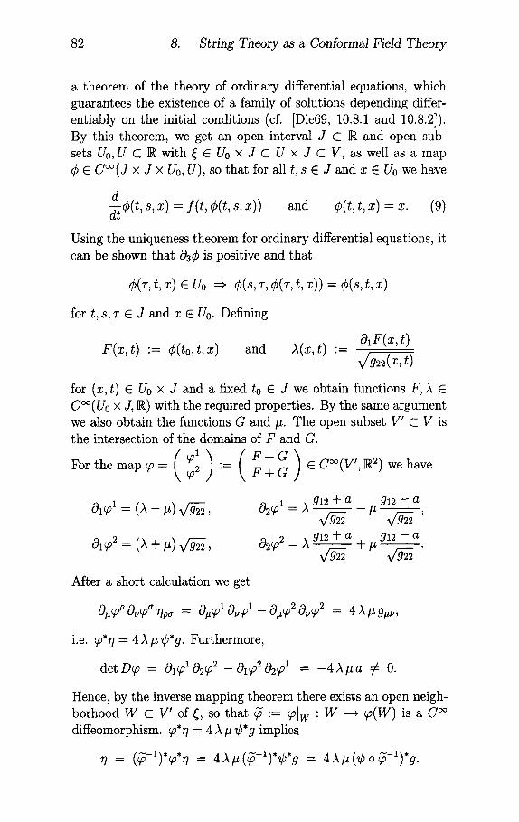
82 8. String Theory as a Con[ormal Field Theory
a theorem of the theory of ordinary differential equations, which guarantees the existence of a family of solutions depending differ- entiably on the initial conditions (cf. [Die69, 10.8.1 and 10.8.2]). By this theorem, we get an open interval J C R and open sub- setsU0, U C R w i t h ~ E U0× J C U × J C V, as well a s a m a p ¢ E C°°(J × J × Uo, U), so that for all t, s E J and x E Uo we have
d d~¢(t , s, x) = f (t, ¢(t, s, x)) and ¢(t, t, x) = x. (9)
Using the uniqueness theorem for ordinary differential equations, it can be shown that 03¢ is positive and that
¢(~, t, ~) e Uo ~ ¢(~, ~, ¢(~, t, ~)) = ¢(~, t, ~)
for t, s, T E J and x E U0. Defining
F(x, t) "= ¢(to, t, x) and A(x, t) "= 01F(x, t)
for (x, t) E Uo × J and a fixed to E J we obtain functions F, A E C°°(Uo × J, R) with the required properties. By the same argument we also obtain the functions G and #. The open subset V' C V is the intersection of the domains of F and G.
For the map ~ = ~2 "- F + G E (V ~, ) we have
Oxv ~ = ( ~ - , ) 4 ~ ,
o ~ = (~ + , ) ~ ,
GQ2(~I : ,~ g12 -~- a
(~2(~2 ,~ g12 q" a = - t - # ~
g12 -- a
v/g22
g12 -- a
v ~ After a short calculation we get
C~tt~ p Ov~ a ?~pa -- Ott~ 1 0 v ~ 1 -- O#(f12 Ov~2 ._ 4 £ # g,~,
i.e. ~'77 = 4 A # ¢*g. Furthermore,
d e t D ~ = 01~ 1 02~ 2 - (~I~P 2~2(~ 1 : - 4 A # a ~ 0.
Hence, by the inverse mapping theorem there exists an open neigh- borhood W C V' of ~, so that ~ "= ~lw " W --~ ~a(W) is a C °o diffeomorphism. ~*~? = 4 A # ¢*g implies
?7 __ ( ~ - 1 ) , ~ , ? ~ __ 4 A # (~-~)*¢*g - 4 A # (¢ o ~ - l ) , g .
8.1 Action Functionals and Equations of Motion for Strings 83
Now ¢ "= ~)o~ -1" ~ ( W ) --+ M is a chart for M with x e ¢ (~(W))
and we have
with f~ : - 1 / ( 2 x / ~ ) . m
By Theorem 8.2 one can choose a local parameterization of the world sheet in such a way that
h = f~2~ = f~2 ( - 1 \ 0
0 1/ This fixing of h is called conformal gauge. Even after conformal gauge fixing a residual symmetry remains: it is easy to see that Sp(x) in conformal gauge is invariant with respect to conformal transformations on the world sheet. In this manner, the conformal group Conf(IR 1'1) -~ Diff+(S) × Diff+(S) turns out to be a sym- metry group of the system, even if this holds only on the level of "constraints". In any case, the classical field theory of the bosonic string can be viewed as a conformally invariant field theory.
To simplify the equations of motion and, furthermore, to present solutions as certain Fourier series, we need a generalization of The- orem 8.2, stating that (in the case of closed strings, to which we restrict our discussion here) there exists a conformal gauge not only in a neighborhood of any given point, but also in a neighborhood of a closed injective curve (as a starting curve for the "time T -- 0"). The existence of such isothermal coordinates can be shown by the same argumentation as Theorem 8.2. Finally, for the variation in the conformal gauge, it can be assumed that isothermal coordinates exist on the rectangle
Q = [0, 2.] × [0, 2.]
and that a ~ x(0, a), a E [0, 27r] describes a simple closed curve. This is possible at least up to an irrelevant distortion factor (cf. [Die89]).
T h e o r e m 8.3 The variation of SNc or Sp in the conformal gauge leads to the equations of motion on Q = [0, 2~r] x [0, 2r]: These are the two-dimensional wave equations
O~x - O~x = O resp. x ~ - x ~ = O
84 8. String Theory as a Conformal Fidd Theory
with the constraints
<~, ~> - o = <~, ~> + <~, ~ > ,
imposed by the conformal gauge.
(x~, x~) < 0.
By x~ we denote the partial derivative of x = X(T, a) with respect to a (i.e. T := q0, a := ql), and (v, w) is the inner product (v, w) - v~'w~'71~,~, for v, w E R D.
P r o o f To derive the equations of motion and the constraints we start by writing Sp in the conformal gauge h = f]2r/:
s~(~) = s~(~, ~ ) = ((00x, Ooy> - (01x, 01y>)dq°dq 1.
For y • Q --+ R D and suitable boundary conditions YloQ = 0 we have
O Sp(x + ey) e=0
m
2
= ~ f Q
(((90 x, 00y) -- (01X, 01y)) dq°dq ~
<011 x - - ~00 x , Y) dq°dq I
(integration by parts). This yields
011 x -- (900 x -- 0
as the equations of motion in the conformal gauge.
Because of the description of the metric h by h = $gl with A > 0 i.e.
Ah = A(h~j) = (x,, x~) (x,, x,) '
the gauge fixing h - f~2r/implies the conditions
<~, ~> = o, <~, ~> = - <~, ~> > o.
m
The constraints are equivalent to the vanishing of the energy-mo- mentum T, which is defined by
1 Tij = (xi, x j ) - -~hijh kl (xk ,xl) , i , j , k , l e {T,a}
8.1 Act ion Functionals and Equations of Motion for Strings 85
(see (7) and cf. [GSW87, p. 62ff]).
The solutions of the two-dimensional wave equations are
o) = - o) + + o)
with two arbitrary differentiable maps xR and X L on Q with values in R D. For the closed string we get on Q := [0, 2zr] x [0, 2zr] (i.e. X(T, a) = X(T, a + 2zr)) the following Fourier series expansion
X~R (T -- i f) = 1 # 1 # i 1 e - i n ( r - a ) + - + E. o
X~L (T + 0") = 1 it 1 # (T "~- 0") -t- i l - ~ e - i n ( r + a ) ~Xo + ~ P o ~ ~n#O "~ n • (10)
Xo and Po can be interpreted as the center of mass and the center of momentum respectively, while c~ -~ , a . are the oscillator modes of the string. X L and X R are viewed as ,,left movers" and "right movers". We have x0 ~, P0" E R and a ~.,a m-~ E C. -~a m is not the
v For but completely independent of a m complex conjugate of am, X R and X i to be real, it is necessary that
(a.")* = (_.)a" and (~.")* = (~"_.) (11)
holds for all # E { O , . . . , D - 1 } and n E Z \ {0}, where c ~ c* 1 pU The denotes the complex conjugation. We let ao ~ "= ~ := agW~ o.
x = XL + XR with (10) can be written as
z(a, ~) = z o + 2 i 1 (a.e_i.(~_.) + ~.e_i.(~+.)) "
n
Hence, arbitrary a . , a--~, xo, po with (11) yield solutions of the one- dimensional wave equation. In order that these solutions are, in fact, solutions of the equations of motion for the actions SNc or Sp, they must, in addition, respect the conformal gauge. Using
1 - 1 L. "= ~ ~ (ak, an-k) and L. := ~ y ~ {~, ~ . -k) for n E Z,
kEZ kEZ
the gauge condition can be expressed as follows:
L e m m a 8.4 A parameterization X(T, a) = XL(T -- a) + XR(T + a) of the world sheet with XR, XL as in (10) and (11) gives isothermal coordinates i f and only if L . = L . = 0 for all n E Z.

86 8. String Theory as a Conformal Field Theory
Proof We have isothermal coordinates iff
(z,- + z~, z r + z, ,) = (z~. - z,~, z,. - z,,) = O.
Using the identities
2 - i n ( r - a ) X r - - X a = 4VQ-~ y ~ ane and
nEZ
2 z~ + z . = ~ y ~ . e -~"('+~)
nEZ
we get
I 0 ~Xr -- xa, xr -- Xa)
nqZ kEZ
mEZ n + k = r n
n + k = m
-: > V m E z ' y ~ ( a . _ k , ak ) = o
kEZ
-,' ',- V m E Z ' L m = O .
The same argument holds for x~ + x~ and Lm. I
Altogether, we have the following:
Theorem 8.5 The solutions of the string equations of motion are the functions
x(~-, ~) = zo+ V~ra 2---a°T -~ ~ i .~#o nl (OLne_in(r_a) "4- -~n e-in(r+a))
for which the conditions (11) and L~ = L~ = 0 hold.
For a connection of the energy-momentum tensor T of a conformal field theory with the Virasoro generators Ln and Ln we refer to Sect. 9.2, (22).
8.2 Quantization 87
The oscillator modes a~ and am are observables of the classical system. Obviously, they are constants of motion. Hence, one should try to quantize the a~, a-~.
In order to quantize the classical field theory of the bosonic string one needs the Poisson brackets of the classical system:
V { ~ , ~.} = ~ , . - ~ + . = {~,-'~.},
{ ~ , ~ } = o, V
{;o~,~o} = , . ' , {~, ~o}" = {~, ~,} = { ~ , - ~ } = 0,
for all #, ~ E {0 , . . . , D - 1} and m, n E Z (here and in the following we set 4 ra = 1).
L e m m a 8.6 For n, m E Z one has
{Lm, L.} = i ( n - m)Lm+n, (Lm, L.} = i ( n - m)Lm+.,
and (Lm, Ln)=O.
This follows from the general formula
{AB, C} = A {B, C} + (A, C} B
for the Poisson bracket.
8.2 Quantization
The Poisson brackets of the (a~) are those of an infinite-dimensional harmonic oscillator. In canonical quantization, the Poisson brackets are replaced with commutators
{ . , . } : ; - i [ . , . ] ,
A
while the observables f are replaced with operators f"
[f, -
A
For short, we write f instead of f. After quantization we have
[a~, a~] = m ~+.~ 77 ~ and [x~, p~] = it/"~.
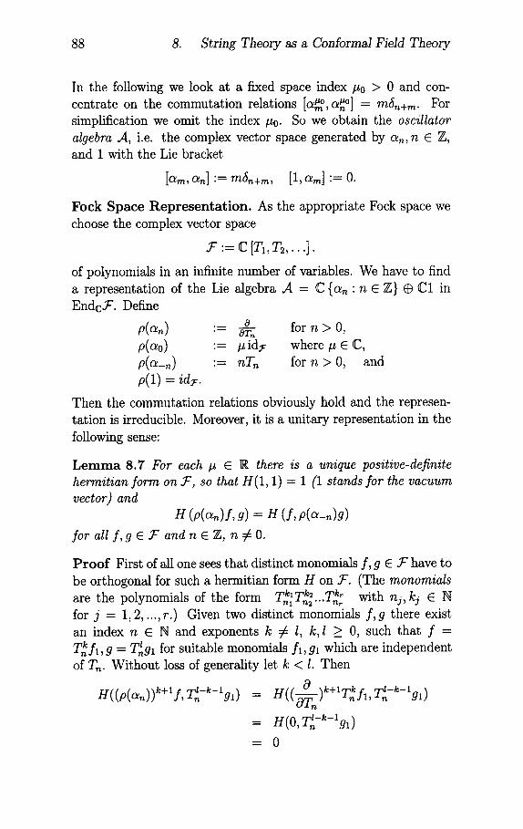
88 8. String Theory as a Conformal Field Theory
In the following we look at a fixed space index #0 > 0 and con- centrate on the commutation relations [a~, a~ °] = mSn+m. For simplification we omit the index #0. So we obtain the oscillator algebra j[, i.e. the complex vector space generated by an, n E Z, and 1 with the Lie bracket
. = [1, . = 0 .
Fock Space R e p r e s e n t a t i o n . As the appropriate Fock space we choose the complex vector space
U "= C [TI, T2, . . . ] .
of polynomials in an infinite number of variables. We have to find a representation of the Lie algebra A = C {a~ : n E Z} @ C1 in Endc~-. Define
o for n > 0, p(an) : = o r .
p(ao) := # idy where # E C, p(a-n) := nTn for n > 0, and p(1) = ids:.
Then the commutation relations obviously hold and the represen- tation is irreducible. Moreover, it is a unitary representation in the
following sense:
L e m m a 8.7 For each # E ]R there is a unique positive-definite hermitian form on .T, so that H(1, 1) = 1 (1 stands for the vacuum vector) and
H (p(a~)f, g) = H (f, p(a_~)g)
for all f , g E jr and n E Z, n ~ O.
P r o o f First of all one sees that distinct monomials f, g E ~" have to be orthogonal for such a hermitian form H on ~'. (The monomials
. . T k~ w i t h n j , kj E N are the polynomials of the form Tnk~Tnk~ . ,,~ for j = 1, 2, ..., r.) Given two distinct monomials f, g there exist an index n E N and exponents k ~ l, k, 1 >_ 0, such that f =
k l Tn f l , g = T~gl for suitable monomials fl, gl which are independent of Tn. Without loss of generality let k < I. Then
=
= H(0, ml-k-11~ gl)
= 0
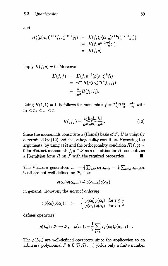
8.2 Quantizat ion 89
and
H((p(an))k+l f,,.,-,t-k-, , In gl) = H ( I , (p(~_.) V l-k- lgl) )
= H ( I , k+l,-,-,t n lug1)
= g ( f , g)
imply H ( f , g) = O. Moreover,
H(f,:) = H ( I , n - k (p (an ) ) k f l )
n - k H k k = (p(an) TnI1,11) k~
-- ~-~H(f l , f l ) .
Using H(1 1) = 1, it follows for monomials f = Tk~T k2 T k" with - n l "" n 2 " " " n r
n l < n2 < . . . < n r
kl !k2!...kr! U ( f , f) = ~-~;-~;:::-~, . (12)
Since the monomials constitute a (Hamel) basis of : ' , H is uniquely determined by (12) and the orthogonality condition. Reversing the arguments, by using (12) and the orthogonality condition S ( f , g) = 0 for distinct monomials f, g E :" as a definition for H, one obtains a Hermitian form H on ~" with the required properties. II
1 1 The Virasoro generators Ln = 5 ~ k e z a~:an-k = "i ~-~k~Z an-kak itself are not well-defined on .F, since
P(ak)P(a.-k) # P(~n-k)P(ak),
in general. However, t h e n o r m a l ordering
p ( . , ) p( j) " := { p(-,)p(-j) p(,j) p(,,)
for i_< j for i > j
defines operators
p(Ln) " 3 z --+ jz, 1
kEZ
• )..
The p(Lm) are well-defined operators, since the application to an arbitrary polynomial P E C IT1, T2,...] yields only a finite number
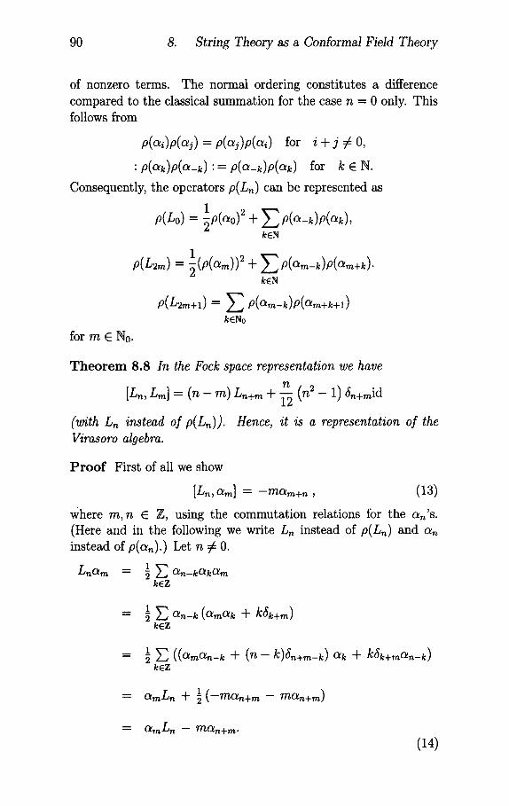
90 8. String Theory as a Conformal Field Theory
of nonzero terms. The normal ordering constitutes a difference compared to the classical summation for the case n = 0 only. This follows from
p(ai)p(aj) = p(aj)p(ai) for i + j ~ O,
: p(ak)p(a-k):= p(a-k)P(ak) for k E N.
Consequently, the operators p(L.) can be represented as
1 9 p(Lo) = -~p(ao) + E p ( a - k ) p ( a k ) ,
kEN
1 p(L2m) = -~(p(am))2 + E p(am-k)p(am+k).
kEN
p(L2m+I) = ~ P(am-k)P(~m+k+l) kENo
for m E No.
T h e o r e m 8.8 In the Fock space representation we have n
[Ln, Lm] = ( n - m)Ln+m + -~ (n 2 - 1) 5.+mid
(with L. instead of p( Ln ) ). Hence, it is a representation of the Virasoro algebra.
P r o o f First of all we show
[Ln, am] = - m a r e + . , (13)
where m, n E Z, using the commutation relations for the an's. (Here and in the following we write L~ instead of p(L.) and ~ . instead of p(an).) Let n # 0.
1 E OLn-kOlkOlm L.am - kEZ
2 kEZ
1- E + + 2
kEZ
1 = amL. + -~ (-ma~+m - ma.+m)
- - Olm L n -- ?nOLn+ m.
(14)
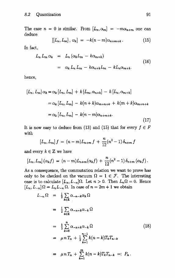
8.2 Quantization 91
The case n = 0 is similar. From [Ln, a,n] = -man+m one can deduce
[[L~, Lm], ak] = - k ( n - m)an+m+k . (15)
In fact,
Ln Lm ak Ln (akL~ - kam+k)
ak Ln Lm - kan+kLm - kLnam+k. (16)
hence,
[L., Lm] ak = ak [L., Lm] + k [Lm, a.+k] - k [L., am+k]
= ak [Ln, Lm] - k(n + k)am+n+k + k(m + k)a,,,+n+k
= ak [Ln, L~] - k(n - m)a.+m+k. (17)
It is now easy to deduce from (13) and (15) that for every f 6 F with
n [Ln, Lm] f = (n - m)Ln+,n f + --i~(n 2 - 1)5.+,n f
and every k E Z we have
n [L., Lm] (ak f ) = ( n - m ) L . + ~ ( a k f ) + -i~(n 2 -- 1)5.+,n (at:f) .
As a consequence, the commutation relation we want to prove has only to be checked on the vacuum ~t = 1 e ~'. The interesting case is to calculate [L., L_.]12. Let n > 0. Then L.gt = 0. Hence [L., L_.] Ct = L .L_n ft. In case of n = 2m + 1 we obtain
1 E a_, -kak k6Z
1 f~ "2 E Ol'-n+kOl-k k6_Z
n
= ! a - . + k a - k gt 2
k=O n-1
1 = # n T. + -~ ~ k(n - k)TkT._k k=l
(18)
m
# n 7'. + ~ k(n - k)TkT._k =: Pn. k=l
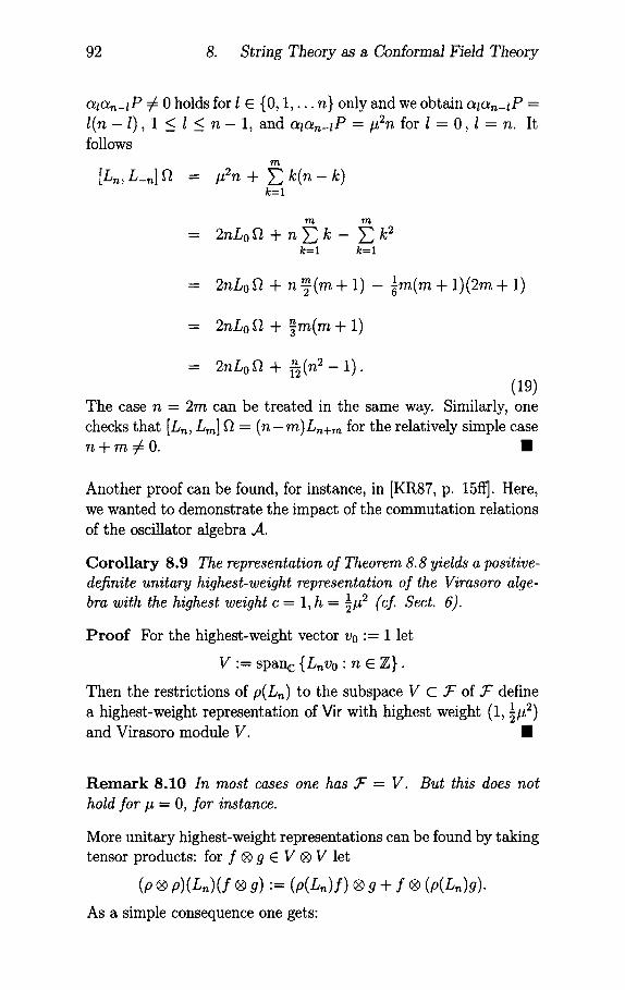
92 8. String Theory as a Conformal Field Theory
ala~-lP ~ 0 holds for I E (0, 1 , . . . n} only and we obtain alc~_lP = l ( n - l ) , l __ l _< n - l, and ala~_tP = #2n for l = O, l = n. It follows
m
[L~,L_n] ~ = #2n + E k ( n - k) k = l
m m
2nLo~ ÷ n ~ k - ~ k 2 k = l k = l
m lm(m + 1)(2m + 1) = 2nLof~ + n T ( m + l ) - g
= 2nLo~ + ~ m ( m + 1)
- 2sLogS+ ~ ( n 2 - 1 ) . (19)
The case n - 2m can be treated in the same way. Similarly, one checks that [in, im] ~ = ( n - m ) i n + m for the relatively simple case n + m ~ O , m
Another proof can be found, for instance, in [KR87, p. 15fl~. Here, we wanted to demonstrate the impact of the commutation relations of the oscillator algebra ,4.
C o r o l l a r y 8.9 The representation of Theorem 8.8 yields a positive- definite unitary highest-weight representation of the Virasoro alge-
1#2 bra with the highest weight c = 1, h = ~ (cf. Sect. 6).
P r o o f For the highest-weight vector v0 := 1 let
V "= span c {L~vo 'n E Z}.
Then the restrictions of p(Ln) to the subspace V C ~" of ~" define 1#2~ a highest-weight representation of Vir with highest weight (1, ~ j
and Virasoro module V. II
R e m a r k 8.10 In most cases one has jz = V. But this does not hold for # = O, for instance.
More unitary highest-weight representations can be found by taking tensor products: for f ® g E V ® V let
(p ® p)(Ln)(f ® g) := (p(Ln)f) ® g + f ® (p(L~)g).
As a simple consequence one gets:
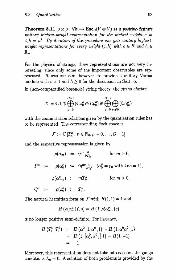
8.2 Quantization 93
T h e o r e m 8.11 p ® p : Yir -~ Endc(V ® V) is a positive-definite unitary highest-weight representation for the highest weight c = 2, h = #2. By iteration of this procedure one gets unitary highest- weight representations for every weight (c, h) with c E N and h E ]~+.
For the physics of strings, these representations are not very in- teresting, since only some of the important observables are rep- resented. It was our aim, however, to provide a unitary Verma module with c > 1 and h > 0 for the discussion in Sect. 6.
In (non-compactified bosonoic) string theory, the string algebra
D-1 D-1
#=0 #=0 m#0
with the commutation relations given by the quantization rules has to be represented. The corresponding Fock space is
$" := C[T2"n E No,# = O , . . . , D - 1]
and the respective representation is given by:
o form >0 , p(~m) "= ~"~or~
0 P" "= p(ao ~) "= ip'~O-~o (ao ~ = po with 4 ra = 1),
p ( ~ ) .= roTe for m > 0,
Q" := p(~o") = To ~.
The natural hermitian form on ~" with H(1, 1) = 1 and
H (p(a~)f, g) = H (f, p(a~_m)g)
is no longer positive semi-definite. For instance,
. (vo, ff) = H (o/°11, o/°11) = H (1, o~1°o/° 11)
= H (1, [a °, a°l] 1) = H ( 1 , - 1 )
"-- - - 1 o
Moreover, this representation does not take into account the gauge conditions L~ = 0. A solution of both problems is provided by the
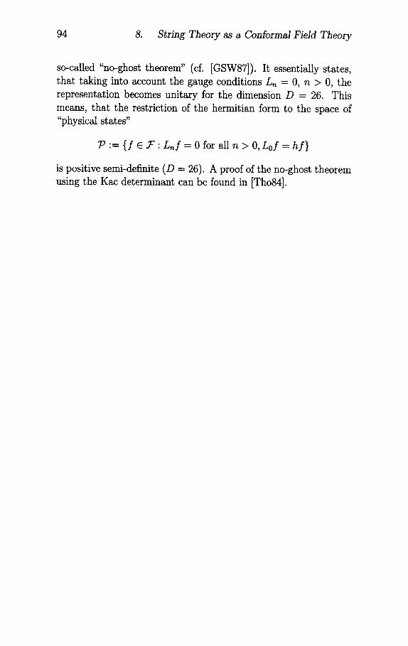
94 8. String Theory as a Conformal Field Theory
so-called "no-ghost theorem" (cf. [GSW87]). It essentially states, that taking into account the gauge conditions Ln = 0, n > 0, the representation becomes unitary for the dimension D = 26. This means, that the restriction of the hermitian form to the space of "physical states"
7 ) "= { f E .T" Lnf = 0 for all n > 0, Lof = h f }
is positive semi-definite (D = 26). A proof of the no-ghost theorem using the Kac determinant can be found in [Tho84].
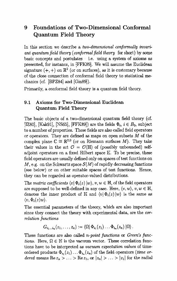
Foundations of Two-Dimensional Conformal Quantum Field Theory
In this section we describe a two-dimensional conformally invari- ant quantum field theory ( conformal field theory for short) by some basic concepts and postula tes- i.e. using a system of axioms as presented, for instance, in [FFK89]. We will assume the Euclidean signature (+, +) on R 2 (or on surfaces), as it is customary because of the close connection of conformal field theory to statistical me- chanics (cf. [BPZ84] and [Gin89]).
Primarily, a conformal field theory is a quantum field theory.
9.1 Axioms for Two-Dimensional Euclidean Quantum Field Theory
The basic objects of a two-dimensional quantum field theory (cf. [IZ80], [Kak91], [NS65], [FFK89]) are the fields ¢,, i e B0, subject to a number of properties. These fields are also called field operators or operators. They are defined as maps on open subsets M of the complex plane C ~ R 2'° (or on Riemann surfaces M). They take their values in the set (9 = O(]E) of (possibly unbounded) self- adjoint operators on a fixed Hilbert space IE. To be precise, these field operators are usually defined only on spaces of test functions on M, e.g. on the Schwartz space S(M) of rapidly decreasing functions (see below) or on other suitable spaces of test functions. Hence, they can be regarded as operator-valued distributions.
The matrix coefficients (v I ~ ( z ) Iw), v, w e ]HI, of the field operators are supposed to be well-defined in any case. Here, (v, w}, v, w E ]E, denotes the inner product of H and (v I Oi(z)Iw) is the same as
The essential parameters of the theory, which are also important since they connect the theory with experimental data, are the cor- relation functions
C i , . . . i , . , ( Z l , . . . , Z n ) : -" (a I (I)il(Zl)... O i n ( Z n ) l a } .
These functions are also called n-point functions or Green's func- tions. Here, gt E IE is the vacuum vector. These correlation func- tions have to be interpreted as vacuum expectation values of time- ordered products ¢i, (z l ) . . . ~,~(z~) of the field operators (time or- dered means Re z~ > . . . > Re Zl, or Iz~l > . . . > Iz~[ for the radial
96 9. Two-Dimensional Conformal Q u a n t u m Field Theory
quantization). They usually can be continued to
M~ "= { ( Z l , . . . , Zn) ~-- Cn 'z i ~ zj for i ~ j } ,
the space of configurations of n points. (To be precise, they have a
continuation to the universal covering M~ of M~ and thus they are no longer single valued on M~, in general. In this manner, the pure braid, group P~ appears, which is the fundamental group rl(M~) of Mn.) For simplification we will assume in the formulation of the axioms, that the Gil...i~ are defined on M~.
The positivity of the hermitian form, i.e. the inner product of H, can be expressed by the so-called reflection positivity of the correlation functions. This property is defined by fixing a reflection a x i s - which typically is the imaginary axis in the simplest case - and requiring the correlation of operator products of fields on one side of the axis with their reflection on the other side to be non-negative (cf. Axiom 3 below).
Now, the two-dimensional quantum field theory can be described completely by the properties of the correlation functions using a system of axioms. The field operators and the Hilbert space do not have to be specified a priori, they are determined by the correlation functions.
To state the axioms we need a few notations:
M + := { ( z l , . . . , z ~ ) C M n ' R e z j > O f o r j = l , . . . , n }
So+ := C 8+ "= {f C 8 ( C ~ ) ' S u p p ( f ) C M +} .
Here, S(C ~) is the Schwartz space of rapidly decreasing smooth functions, i.e. the complex vector space of all functions f E C°°(C ~) for which
sup sup [O~f(x)l (1 + Ix[2) k < oe, [aI<_p Z~-~ 2n
for all p, k E N. We have identified the spaces C n and R 2n and have used the real coordinates x - (x l , . . . , x2=) as variables. 0 a is the partial derivative for the multi-index a E N 2~ with respect to x. Supp(f) denotes the support of f , i.e. the closure of the set
e # 0}.
It makes sense to write z E C as z = t + iy with t, y E R, and to interpret -2 - t - iy as a quantity not depending on z. In this sense
9.1 A x i o m s for Two-Dimensional Euclidean Q F T 97
one sometimes writes G(z,-2) instead of G(z) , to emphasize that G(z) is not necessarily holomorphic. In the notation z = t + iy , y is the "space coordinate" and t is the (imaginary) "time coordinate".
The group E - E2 of Euclidean motions, i.e. the Euclidean group (which corresponds to the Poincar~ group in this context) is gener- ated by the rotations
r~ " C ---, C, z ~ e~z , a E R,
and the translations
ta:C---,C, z ~ z + a , a(EC.
Further MSbius transformations are the dilatations
d~ :C- - - ,C , z ~ e ~z, T E R ,
and the inversion
i "C - - .C, z~-~ Z 1 - , zeC\{0}.
These conformal transformations generate the M5bius group Mb (cf. Sect. 2.3). The other global conformal transformations (cf. Definition 2.7) are generated by Mb and the t ime reflection
O : C - - - , C , z = t + iy ~-, - t + iy = --2.
Osterwalder-Schrader Axioms ([OS73], [OS751)
Let Bo be a countable index set. For multi-indices ( i l , . . . , in) E B~ we also use the notation i = i l . . . i n = ( i l , . . . , i~) . Let B = UneNo B~. The quantum field theory is described by a family (Gi) ies of continuous and polynomially-bounded correlation func- tions
Gi,...i, :M~ ~ C, G~ = 1,
subject to the following axioms:
Axiom 1 (Locality) For all ( i l , . . . , in ) E B~, (zl , . . . , z~) E M~ and every permutat ion ~ : { 1 , . . . , n} ~ { 1 , . . . , n} one has
Gi, .... ,in ( Z l , . . . , Z n ) - Gi~( , ) . . . i ,~ (n) (Z l r (1 ) , . . . , Z l r ( n ) ) .
98 9. Two-Dimensional Conformal Quantum Field Theory
A x i o m 2 (Covar iance) For every i E Bo there are conformal weights hi, hi E R (hi is not the complex conjugate of hi, but com- pletely independent of hi), such that for all w E E and n >__ 2 one has
G i x . . . i . ( z l , - e l , . . . , z , , )
- aix...in (Wl , W l , • • • , Wn, W-n),
with wj "= w(zj), Nj := w(zj), hj := hij. (20)
m
Here, si := h i - hi is called the conformal spin for the index i and di := hi + hi is called the scaling dimension.
Furthermore, we assume
h i - h i , h i + h i E Z , i E B 0 .
As a consequence, there do not occur any ambiguities concerning the exponents, and
- 1
hi, hi E ~Z.
See Hawley/Schiffer [HS66] for a discussion of this condition.
The covariance of the correlation functions formulated in Axiom 2 corresponds to the transformation behavior of tensors under change of coordinates. It severely restricts the form of 2-point functions and 3-point functions. Because of the covariance with respect to translations, all correlation functions Gi~...i, for n ___ 2 depend only on the differences zij "= zi - zy, i ¢ j , i , j E {1 , . . . , n}. Typical 2-point functions Gi~ix = G, which satisfy Axiom 2, are
G = const, with h = h = 0
G(zl,-Zl, z2, ~2) - Cz122z122 with h = h = 1
G(Zl, z2) - CZl24 with h = 2, h = 0.
A general example is
V(Zl, z2) - Cz122h-z122h - 1
with h, h E ~Z. z
D
Hence, for the case h = h:
G(Zl, Z l , z2, ~2) - - C Iz121-4h = C Izi 1-2d
9.1 Axioms t'or Two-Dimensional Euclidean QFT 99
Typical 2-point functions G = Gill2 with il ~ i2, for which Axiom 2 is valid, are
G(Zl, Zl, Z2, Z2) -- C z12 hi z12 h2 z12 hi z12 h2.
All these examples are also MSbius covariant.
For the function F = Gixi~ with
F ( z 1 , Zl , z2, Z2) - - - - l o g 1z1212 Axioms 1 and 2 hold as well (with arbitrary h, h, h = h). How- ever, this function is not MSbius covariant because one has e.g. for w(z) = e'z, T # O, and in the case h = h # 0:
1] 7;z(ZJ) Tz(Zj) j=l
_ _ - 12. - (e~)2h+2h( - log e 2r [zx2l 2) :fi --log [zx2
In particular, F is not scaling covariant in the sense of Axiom 4 (see below). A typical 3-point function is
G(Zl, Zl, Z2,-z2, z3,-z3)
-hi-h2-}-h3 -h2-h3 -.[-h l - h3 -h l +h2 (21 ) --- Z12 Z23 Z13
~12hI- -h2-~-h3~23h2-h3-~-hl~13h3-hl -~-h2
as can be checked easily. It is not difficult to see, that this 3-point function is also M5bius covariant.
A x i o m 3 (Ref lec t ion Pos i t iv i ty ) There is a map . " Bo ~ Bo with .2 = idBo and a continuation • • B ~ B, i ~-+ i*, so that
1. G~(z) = G~.(O(z)) = G, . ( -z*) for i e B, where z* is the complex conjugate of z.
2. (f_., f_.) > 0 for all f_. E S_ +.
Here S + is the set of all f = (fi)~eB with fi 6 $+ for i e B~ and
fi ~ 0 for at most finitely many i E B. ( f_, f_) is defined by
i,jEB n,m +m
"f,(z)*fj(w)dnzdmw.
100 9. Two-Dimensional Conformal Quantum Field Theory
L e m m a 9.1 (Reconstruction of the Hilbert Space) Axiom 3 yields a positive semi-definite hermitian form H on S_ + and hence the Hilbert space ttI as the completion of S_ +/ker H with the inner product ( , ) .
We now obtain the field operators by using a multiplication in S_. Indeed, ¢i for i E B0 shall be defined on a suitable subspace Di C S + with values in a space of operators. To do this, the ~ ( f ) for f E Di have to be determined as operators on ]E. Given f E Di C S + and g E _S +, g = (gi)ieB, let the element f x g ( = ¢i(f) , the expected value of ¢ at f) be defined by
(f >< g__),x...,.+x (Zl , . . . , Zn+l) :-" f(Zl)~ixigi2...in+l (Z2,... , Zn+l).
It can be shown (cf. [OS731,[OS751) that the map ¢ , ( f ) • g ~ f x g
is defined for sufficiently many g E S_ +. Furthermore, there is an F/E IE (namely f~ = f, with f0 = 1 and fi = 0 for i ¢ t~) with the following properties:
T h e o r e m 9.2 (Recons t ruc t ion of the Field Opera to r s )
1. ~ ( f ) • g ~ f x g is a linear operator on ~I and ~ " D~ ----, (9 is a field.
2. For convergent sequences
fk---*5~, f k E D i , z E { w E C ' R e w > O }
one has
~i(z) E O, and
¢i(z)g := lira qh(f)g, - - k - - - * ~ - -
(al ~ , (z) la) := lim (a I ff,(fk)[a) k--'-~oo
is a well-defined continuous and polynomially-bounded func- tion on
{w E C" Re w > 0}.
3. For Re z, > . . . > Re Zl one has
<al ~, (z , ) . . . ~,(z.) la> = a,, . . . , . (z, , . . . ,z.).
9.2 Conformal Fields and the Energy-Momentum Tensor 101
~. From Axiom 2, a representation of E in IE with respect to self-adjoint operators can be determined. ~ is invariant with respect to this representation.
Further, the C~...~, (z~, ~ , . . . , Zn, ~n) are holomorphic in M > × M >, where
M > := {z E M + ' R e z n > ... > Rezl > 0}.
They can be analytically continued to a domain N C C ~ × C n.
Similar results are true for other regions in C instead of the right half plane
{w E C" Rew > 0},
e.g. for the disc (radial quantization). In this case the points z E C are parameterized as z - e ~+ia with the time variable T and the
space variable ~, which is cyclic. The time order becomes Iznl > • . . > Iz l.
9.2 Confo rma l Fields and the E n e r g y - M o m e n t u m Tensor
A two-dimensional quantum field theory with field operators
(¢i)i B0,
satisfying Axioms 1 to 3 is a conformal field theory if the following conditions hold:
• the theory is covariant with respect to dilatations (Axiom 4),
• it has a divergence-free energy-momentum tensor (Axiom 5) and
• it has an associative operator product expansion for the pri- mary fields (Axiom 6).
Ax iom 4 (Scaling Covariance) The correlation functions
Gi, i E B \ B1,
satisfy (20) also for the dilatations w(z) = e ~z, T e R. Hence
z , ) = +h.
for ( z l , . . . , z~) e M, i = ( i l , . . . , in ) and hj = hij.
102 9. Two-Dimensional Conformal Quantum Field Theory
L e m m a 9.3 In a quantum field theory satisfying Axioms 1 to 4, any 2-point function Gij has the form
= C z -(h~+hj ) Gij(Zl, Z2) i j l2 )~12 (hi+hi (Zl2=Zl--Z2)
with a suitable constant Cij E C. Hence, for i = j,
m
aii(Zl, z2) = ~iiz122hz122h.
Similarly, any 3-point function Gijk is a constant multiple of the function G in (21)" Gijk = Cijk G with Cijk E C. In particular, the 2- and 3-point functions are completely determined by the constants c j, C jk.
P r o o f As a consequence of the covariance with respect to trans- lations, G := Gij depends only on z12 = Zl - z2, i.e. G(zl, z2) = G~3(Zl- z2, 0). For z = re ~ = e~e ~ one has G(z, 0) = G(e~+~l, 0). From Axioms 2 and 4 it follows
G(1, O) = (e'+i'~) h' (e"-i~') h' (e~+i'~) h~ (e~-i~) hj G(e'+i'~l, 0).
This implies G(z, O) = Z-(h'+hJ)-5-(h'+hJ)G(1, 0), C "= G(1, 0). A similar consideration leads to the assertion on 3-point functions. II
The 4-point functions are less restricted. [GinS9]) that they have the form
It can be shown (cf.
G(Zl, Z2, Z3, Z4) = F (r(z), r(z) - - h - - ) + ~ h
i<i i<i
n
where h = h l + h2 + h3 + h4 and correspondingly for h, and where F is an arbitrary holomorphic function in the cross-ratio
:= (z,2z34)/(z13z24)
of the Z12 , Z34 , Z13 , Z24 and in r(z).
Analogous statements hold for the n-point functions, n >_ 5. As an essential feature of conformal field theory we observe that the form of the n-point functions can be determined by using the conformal symmetry. They turn out to be Laurent monomials in the z~j, ~ j up to a factor similar to F.
9.2 ConformM Fields and the Energy-Momentum Tensor 103
Axiom 5 (Existence of the Energy-Momentum T e n s o r )
Among the fields (~)~eSo there are four fields Tg~, # , v e {0, 1}, with the following properties
• T,. = T ~ . , T..(z)* = T~,. (o(~)),
0 Or:= O • OoT, o + 01Tl~t = 0 with 0o "= ~, ~ ,
• d (Tt,.) = hg, + hg, = 2, s(Too - Tll -4- 2iT01) = +2 .
Theorem 9.4 (Liischer-Mack)[LM761 The axioms 1 to 5 imply
• tr(T,~) = T~ = Too + T l l - - 0.
1 (Too-T1 2iTol) is independent Th erefo re T : = Too - iTol = -~ t -
of-2, i.e. OT = O. Hence, T is holomorphic . In the same way T := Too +iTol is independent of z, anti-holomorphic. For the c o ~ p o ~ d i ~ g co~brmal ~ g h t ~ ~ ha~ h(T) = -~(T) = 2 and h(T) = h(T) = O.
• By
L_. "= ~ i= 1 ~n+l d(, L_. "= ~n+l d ( ( 2 2 ) 21ri I=1 m
the operators L~, L~ on ]E are defined, which satisfy the com- mutation relations of two commuting Virasoro algebras with the same central charge:
C 2 [L~, Lm] = (n - m)L.+m + -~n(n
- - C 2
[-Ln,-Lm] = (n - mlL.+m + -i~n(n
= o
- l)6~+m
- 1)~.+m
• The representations of the Virasoro algebra defined by Ln and L . respectively are unitary: L~* = L_n and Ln = L_~.
Incidentally, the proof given in [LM76] is based on the Minkowski signature.
The Ln, L~ can be interpreted as Fourier coefficients of T, T, since
T(z) = z - T(z) = E ~ -(.+2)~. (23) kEZ kEZ
104 9. Two-Dimensional Conformal Quantum Field Theory
This is how conformal symmetry in the sense of the representation theory of the Virasoro algebra (cf. Sect. 6) occurs in the axiomatic presentation of the conformal field theory. The operators L~, L~ define a unitary highest-weight representation with weights (c,2). Therefore, altogether, we have a unitary representation
Vir x ~/ir --~ Endc(W~,2 ® W~,2).
An important tool in conformal field theory is the operator product expansion of two operators A and B of the form A = ¢(zl) and B = • (z2), where ~, • are field operators. Before we treat operator product expansions in the next subsection let us note that in the case of ¢ = • = T the product T(z~)T(z2) has the operator product expansion
c T(z~)T(z2) ,,~ ~ ( z 1 - z2) -4 -~- 2 ( z 1 - z2)-2T(z2)+ (z 1 - z2) -1 T ( z 2 )
(24) (Here and in the following, we neglect problems of normal ordering for simplicity. The symbol "~" signifies asymptotic expansion, i.e. "=" modulo a regular function R(zl, z2)).
The validity of (24) turns out to be equivalent to the commutation relations of the L~, L~ (see also Theorem 9.4).
9.3 P r i m a r y Fields, Opera tor P roduc t Expansion and Fusion
In the literature on conformal field theory, one often finds the claim, that at least the primary fields have transformation properties as in Axiom 2 for arbitrary holomorphic transformations w = w(z) as well, and that this covariance expresses the conformal symmetry. However, the covariance property (20) for general w only holds "infinitesimally". In fact, this infinitesimal version of (20) leads to the concept of a primary field.
Definition 9.5 A conformal field ¢i, i E Bo, is called a primary field if
[Ln, ¢~(z)] = zn+lO¢i(z) + hi(n + 1)z~,(z) (25)
for all n E Z, where 0 = o (and correspondingly for the -2-depen- dence, which we shall not consider in the following).
9.3 Primary Fields, Operator Product Expansion and Fusion 105
The primary field property can be characterized in the following way: the primary fields are precisely those field operators ~ E B0, which have the following operator product expansion (OPE) with the energy-momentum tensor T:
1 0 h, ~, (z2)+ ~, (z2) (26)
T(Zl)t~i(z2) " ( Z l - z2) 2 Zl - Z20Z2
The invariance required by (25) can also be interpreted as a for- mal infinitesimal version of (20) in Axiom 2 for the transformation w = w(z) = z + z "+1" the existence of a Lie group for Vir and a corresponding unitary representation of this symmetry group (or of a central extension of Diff+(S) according to Sect. 3) by U would imply the formal identity
U(etL")¢'(z)U(e-tL") = dz ] (27)
for wt(z) = z + tz n+l (here we take Ln = --(zn+l) d , cf. Sect. 5.2). Since U is unitary, the globalized formal analogue of (27) for holomorphic transformations leads to (20) for wt"
G,(z) = \ dz a, (wt(z)) .
Applying dlt=o to the equation (27) we obtain
[Ln,¢i(z)]
on the left-hand side and
d 1)zn)h , d dt (1 + t(n + Oi(z) t=o + -~Oi(Wt(Z)) t=O
---- hi(n + 1)znOi(z) -I- z n+l--~zoi(z
on the right-hand side. This discussion might motivate the notion of a primary field, and in particular (25).
The energy-momentum tensor T is not a primary field, as one can see by comparing the expansions (24) and (26), except for the spe- cial case of c = 0 and h = 2.
From a more geometrical point of view, a primary field with h - 1, h = 0 corresponds to a meromorphic differential form.
106 9. Two-Dimensional Conformal Quantum Field Theory
Definition 9.6 In a quantum field theory satisfying Axioms 1 to 5 let
B1 "= {i E Bo "(hi is a primary field}.
The associated conformal family [¢i] for i E B1 is the complex vector space generated by
ebb(z) "= L_,~ (z) . . . L_,N(z)(b~(z )
f o r = (a l , , aN) e N • . . , Ol 1 ~ . . . ~ O~ g > O, w h e r e
f o r z e C. descendants.
(28)
1 / T(() L_n(z) := ~ ( ( _ z)n+ t d(
The operators O~(z) are called secondary fields or
The operators L_n(z) are in close connection with the Virasoro generators Ln because of
1 i T(() L_n = 27ri _ (n+l d( = L_n(O)
(cf. Theorem 9.4). The secondary fields ¢~ can be expressed as integrals as well. For instance, for ~ , k E N,
1 J T(¢) (bk(z) = L_k(Z)~b~(z) = ~-~ (¢ _ z)k+ 1 (b~(z)d¢.
For any fixed z E C the conformal family [~i] of a primary field ¢i defines a highest-weight representation with weight (ci, hi) (cf. Sect. 6) in a natural manner, v := (hi(z) is the highest-weight vector, Lo(v):= hiv, L,~(v)"= 0 for n E N and L_n(v)"= ~ for n E N .
The primary fields of a conformal field theory shall have the fol- lowing operator product expansion (OPE) according to [BPZ84]
• ~(zi)~(z2) ~ ~ C~k(Zl - z2)hk-h'-hJ¢~(z2) (29) kEB1
with constants Cijk which occur in the expression (21) of the 3- point functions (cf. Lemma 9.3). Similar expansions hold for the descendants.
The central object of conformal field theory is the determi- nation of
9.3 Primary Fields, Operator Product Expansion and Fusion 107
m
• the scaling dimension di = hi + hi,
• the central charge ci for the family [if)i]
• and the coefficients Ci,j,k
from the operator product expansion (29) using the conformal sym- metry.
This can be achieved if the O PE (29) is associative. This additional property allows us to determine all 4-point functions Gi~imi4(z,-2), (il, i2, i3, ia) E B14 and to represent them with the aid of so-called (holomorphic and anti-holomorphic respectively) "conformal blocks" y~, F~.
__ ~ s ,
and analogously for the n-point functions.
A conformal field theory can also be defined on arbitrary Riemann surfaces instead of C. Then the $'~, ~ depend only on the com- plex structure of the surface. Finally, they can be considered as holomorphic sections on the appropriate moduli spaces with values in suitable line bundles (cf. [FS87], [KNR94], [TUY89]).
In any case a conformal field theory has to sat isfy- in addition to Axioms 1 to 5 - the following axiom:
A x i o m 6 (Operator Product Expans ion) have the OPE (29). This OPE is associative.
The primary fields
Conc lud ing Remarks:
1. All n-point functions of the primary fields can be derived from the Gi for i E B~.
2. The expansions (29) are the fusion rules, which can be written formally as
× =
16.B1
or, carrying more information, as
l
where Ni~ E No is the number of occurrences of elements of the family [(I)]l in the OPE of ¢i(z)¢~(0).
108 9. Two-Dimensional Conformal Quantum Field Theory
3. A conformal field theory is a rational conformal field theory if B1 is finite and if ci E Q.
4. We have sometimes passed over to radial quantization, e.g. by using Cauchy integrals in Sect. 9.2, for instance
1 / T(ff) L_n(z) = ~ (~ _ z)n+ 1 d~.
@ To construct interesting examples of conformal field theories satisfying Axioms 1 - 6 it is reasonable to begin with string theory. On a more algebraic level this amounts to study Kac- Moody algebras and vertex operators. This subject is sur- veyed e.g. in [Uen95] where an interesting connection with the presentation of conformal blocks as sections in certain holomorphic vector bundles is described (eft also [TUY89]). For other examples, see [FFK89].
9.4 Other Approaches to Axiomatization
In order to fix the foundations of conformal field theory introduced in [BPZ84], Moore and Seiberg proposed the following axioms for a conformal field theory in [MS89]:
A conformal field theory is a Virasoro module
v = G h,)® h-,) iEB1
m
with unitary highest-weight modules W(c~, h,), W(~, h~) (cf. Sect. 6), subject to the following axioms:
P 1. There is a uniquely determined vacuum vector f~ = 10) E V with f~ e W(c~ o, h~o)® W(~io, h~o), h~o = h~o = O. f~ is SL(2, C) × SL( 2, C)-invariant.
P 2. To each vector a E V there corresponds a field ~ , i.a. an operator O~(z) on V, z E C. Moreover, there exists a conjugate ¢~, such that the OPE of @~@~, contains a descendant of the unit operator.
P 3. The highest-weight vectors a = i = vi of W(ci, hi) deter- mine primary fields Oi. Similarly for the highest-weight vectors of W(~,, h,).
9.4 Other Approaches to Axiomatization 109
P 4. G~(z)= (~ l¢~(z~) . . .¢~(z~) I~) , Izll > .. . > Iz~ l, always has an analytical continuation to M~.
P 5. The correlation functions and the one-loop partition functions are modular invariant (cf. [MS89]).
Another axiomatic description of conformal field theory was pro- posed by Segal in [Seg91], [Seg88b] [Seg88a]. The basic object in this ansatz is the set of equivalence classes of Riemann surfaces with boundaries, which becomes a semi-group by defining the product of two such Riemann surfaces by a suitable fusion (cf. Sect. 7).
Friedan and Shenker introduced in [FS87] a different, interesting system of axioms, which also uses the collection of all Riemann surfaces as a starting point.
10 Mathematical Aspects of the Verlinde Formula
The Verlinde formula describes the dimensions of spaces of con- formal blocks (cf. Sect. 9.3) of certain rational conformal field theories (aft [Ver88]). With respect to a suitable mathematical in- terpretation, the Verlinde formula gives the dimensions of spaces of generalized theta functions (cf. Sect. i0.I). These dimensions and their polynomial behavior (cf. Theorem 10.6) are of special interest in mathematics. Prior to the appearance of the Verlinde formula, these dimensions were known for very specific cases only, e.g. for the classical theta functions (cf. Theorem 10.5).
The Verlinde formula has been presented by E. Verlinde in [Ver88] as a result of physics. Such a result is, of course, not a mathemat- ical result, it will be considered as a conjecture in mathematics. However, the physical insights leading to the statement of the for- mula and its justification can be of great help in proving it. Several mathematicians have worked on the problem of proving the Ver- linde formula, starting with [TUY89] and coming to a certain end with [Fal94]. These proofs are all quite difficult to understand.
In this last section of the present notes we want to explain the Verlinde formula in the context of stable holomorphic bundles on a Riemann surface, i.e. as a result in function theory or in alge- braic geometry. Furthermore, we will sketch a strategy for a proof of the Verlinde formula which uses a kind of fusion for compact Riemann surfaces with marked points. This strategy is inspired by the physical concept of the fusion of fields in conformal field the- ory as explained in the preceding section. We do not explain the interesting transformation from conformal field theory to algebraic geometry.
10.1 The Moduli Space of Representations and Theta Funct ions
In the following, S is always an oriented and connected compact surface of genus g = g(S) E N0 without boundary. The moduli space of representations for the group G is
A4 G := Horn (r~ (S), G ) / G .
10.1 111 The Moduli Space of Representations
The equivalence relation indicated by "/G" is the conjugation
g ,,~ g' .,, ,, 3h E G. g = hgh -1.
Theorem 10.1 3d C has a number of quite different interpreta- tions. In the case of G = SU(r) these interpretations can be formu- lated in form of the following one-to-one correspondences (denoted by "~- "):
1. ,M SUrf) =Hom (Tr~ (S), SU(r)) /SU(r) .
Topological interpretation: the set jM sU(r) is a topological in- variant, which carries an amount of information which inter- polates between the fundamental group 7rl(S) and its abelian part
HI (S) = rx (S)/[~r~ (S), ~rx (S)],
the first homology group of S.
2. Jtd sUrf) ~ set of equivalence classes of jqat SU(r)-bundles.
Geometric interpretation: there are two related (and eventu- ally equivalent) interpretations of "flat" SU(r)-bundles; "flat" in the sense of a fiat vector bundle with constant transition functions and "fiat" in the sense of a vector bundle with a flat connection (corresponding to SU(r) in both cases). Two such bundles are called equivalent if they are isomorphic as fiat bundles.
3. 3d sv(~) -~ [-II(S, SU(r)) ~- H 1 (Trl(S), SU(r)).
Cohomological interpretation:/:/1(S, SU(r)) denotes the first Cech cohomology set with values in SU(r) (this is not a group in the non-abelian case) and H 1 (lrl(S),SU(r)) denotes the group cohomology of r l (S) with values in SU(r).
Msv( ) /g.
Interpretation as a phase space: ,4 is the space of differ- entiable connections on the trivial bundle S x SU(r) ---, S, Ao c A is the subspace of fiat connections and ~ is the cor- responding gauge group of bundle automorphisms; i.e.
G c°°(s, suff )).
Ao /g appears as the phase space of a three dimensional Chern- Simons theory with an internal symmetry group SU(r) with respect to a suitable gauge (cf. [Wit89]).
112 10. Mathematical Aspects of the Verlinde Formula
. .M sU(~) ~- moduli space of semi-stable holomorphic vector bundles E on S of rank r with det E = Os.
Complex-analytical interpretation: here, one has to introduce a complex structure J on the surface S such that S equipped with J is a Riemann surface Sj. The vector bundles in the above moduli space are holomorphic with respect to this com- plex structure and the sheaf Os is the structure sheaf on Sj. To emphasize the dependence on the complex structure J on
• s u ( ~ ) S, we denote this moduh space by . A ~ j .
To prove the above bijections "-~" in the cases 2., 3. and 4. is an elementary exercise for understanding the respective concepts. Case 5. is a classical theorem of Narasimhan and Seshadri [NS65] and is much more involved.
In each of these cases, "-~" is just a bijection of sets. However, the different interpretations yield a number of different structures on A4 sv(~). In 1., for instance, M sv(~) obtains the structure of a subvariety of SV(r) 2g/SU(r) (because of the fact that r l (S) is a group of 2g generators and one relation, cf. (33) below), in 4. the set A4 sU(~) obtains the structure of a symplectic manifold and in 5., according to [NS65], the structure of a Kiihler manifold outside the singular points of Ad sU(~).
Among others, there are three important generalizations of Theo- rem 10.1"
• to other Lie groups G instead of SU(r),
• to higher-dimensional compact manifolds M instead of S and, in particular, to K£hler manifolds in connection with 5.
• to S \ {P~,. . . , Pro} instead of S with points P~, . . . , Pm E S (cf. Sect. 10.3) and a suitable fixing of the vector bundle structure near the points P1, . . . , Pm E S.
To begin with, we do not discuss these more general aspects, but rather concentrate on All sU(~). The above-mentioned structures induce the following properties on Ad BU(~)"
Ad sv(~) has a natural symplectic structure, which is induced by the following 2-form w on the affine space
10.1 113 The Moduli Space of Representations
of connections:
w(a, ~) - c £ tr(c~ A/~) (30)
for a, fl e .Al(S,~u(r)) with a suitable constant c e R \ {0}. Here,
tr • su(r) --+ R
is the trace of the complex r x r-matrices with respect to the natural representation. In what sense this defines a symplec- tic structure on A and on Ao/(J will be explained in more detail in the following.
In fact, for a connection A E ,4 the tangent space TA.A of the affine space ,4 can be identified with the vector space Al(S, su(r)) of su(r)-valued differentiable 1-forms. Hence, a 2-form on A is given by a family (WA)Ae.a of bilinear mappings WA on Al(S, su(r))x Al(S, su(r)) depending differentiably on A E A. Now, the map w" Al(S, su(r)) x Al(S, su(r)) ----, C defined by (30) is independent of A E A with respect to the natural trivialization of the cotangent bundle
T*A = A x ¢41(S,~u(r)) *.
Consequently, w with (30) is a closed 2-form. It is non- degenerate since w(c~, fl) = 0 for all ~ implies fl = 0. Hence, it is a symplectic form on ,4 defining the symplectic structure. Moreover, it can be shown that the pushforward of wl~ o with respect to the projection Ao --+ Ao/G gives a symplectic form w~ on the regular part of A0/G. Indeed, Ao/G is obtained by a general Marsden-Weinstein reduction of (A, w) with re- spect to the action of the gauge group G where the curvature map turns out to be a moment map.
This symplectic form w~ is also induced by Chern-Simons theory (cf. [Wit89]). Ao/G with this symplectic structure is the phase space of the classical fields.
• Moreover, on .A4 sU(~) there exists a natural line bundle £: (the determinant bundle) - which is uniquely determined up to isomorphism - together with a connection V on £ whose
114 10. Mathematical Aspects of the Verlinde Formula
curvature is 2riw. With a fixed complex structure J on S, for instance, the line bundle L: has the following description:
I AASU(r ) O ' = [E] e , . , j •dimc H ° (S, E) >_ 1 }
^Asu(~) for which is a Cartier divisor (the "theta divisor") on , . , g , the sheaf
L: = Lo = O(O) = sheaf of meromorphic functions f on Msu(~)
g with ( f ) + O >_ 0
is a locally free sheaf of rank 1. Hence, 1: is a complex line bundle, which automatically is holomorphic with respect to the complex structure on the moduli space induced by J. (H°(S, E) is the vector space of holomorphic sections on the compact Riemann surface S = Sj with values in the holomor- phic vector bundle E and [El denotes the equivalence class represented by E.)
Definition 10.2 The space of holomorphic sections in f k, i.e.
H° (.M SjU ( ~ ) , C.k ) ,
is the space of generalized theta functions of level k E N.
Here, L: k is the k-fold tensor product of L:: £k = L ® . . . ® £ (k-fold). sv(~) Since A~/j is compact, H°(A~t sU(~) f_k g , ) is a finite-dimensional
vector space over C.
In the context of geometric quantization, the space
H°(Msju(~),£)
can be interpreted as the quantized state space for the phase space (A~tsv(~),w), prequantum bundle L: and holomorphic polarization
J. A similar result holds for H°(.MSg U(~), £k). To explain this we include a short digression on geometric quantization (cf. [Woo80] for a comprehensive introduction):
Geomet r i c Quant iza t ion . Geometric quantization of a classical mechanical system proceeds as follows. The classical mechanical system is supposed to be represented by a symplectic manifold (M,w). For quantizing (M,w) one needs two additional geomet- ric data, a prequantum bundle and a polarization. A prequantum
10.1 The Moduli Space of Representations 115
bundle is a complex line bundle L ---, M on M together with a connection V whose curvature is 2riw. A polarization F on M is a linear subbundle F of (i.e. a distribution on) the complexified tangent bundle T M c fulfilling some compatibility conditions. An example is the bundle F spanned by all "y-directions" in M = R 2 with coordinates (x, y) or on M = C ~ the complex subspace of T M c
0 spanned by the directions ~ , j = 1, ..., n. This last example is
the holomorphic polarization which has a natural generalization to arbitrary complex manifolds M. Now the (uncorrected, see (32)) state space of geometric quantization is
z : - {s e r (M, L) : s is covariantly constant on F} .
Here, F(M, L) denotes the g°°-sections on M of the line bundle L and the covariance condition means that V x s = 0 for all local vector fields X : U --, F C T M c with values in F. In case of the holomorphic polarization the state space Z is simply the space H°(M, L) of holomorphic sections in L.
AASU(~) Back to our moduli space , . , j with symplectic form w~, the AASU(~) holomorphic line bundle £ ---, , . ,g and holomorphic polariza-
tion one gets the following: for every k E N, f.k is a prequan- tum bundle of (jt4j sU(~), k w h . ) Consequently, g°(.MSj U(~), £~) is
the (uncorrected) state space of geometric quantization.
In order to have a proper quantum theory constructed by geomet- ric quantization it is necessary to develop the theory in such a way that the state space Z obtains an inner product. By an appropri- ate choice of the prequantum bundle and the polarization one has to try to represent those observables one is interested in as self- adjoint operators on the completion of Z (see [Woo80]). We are not interested in these matters and only wanted to point out that the space of generalized theta functions has an interpretation as the state space of a geometric quantization scheme:
L )
is the (uncorrected) quantized state space of the phase space
(M sv( l kw) J ~
for the prequantum bundle £:k and for the holomorphic polarization l lASU(r )
o n ~ , j .
116 10. Mathematical Aspects of the Verlinde Formula
Before continuing the investigation of the spaces of generalized theta functions we want to mention an interesting connection of geometric quantization with representation theory of compact Lie groups which we will use later for the description of parabolic bun- dles. In fact, to a large extent, the ideas of geometric quantization developed by Kirillov, Kostant and Souriau have their origin in representation theory.
Let G be a compact, semi-simple Lie group with Lie algebra g and fix an invariant non-degenerate bilinear form < , > on g by which we identify g and the dual g* of g. For simplicity we assume G to be a matrix group. Then G acts on g by the adjoint action
Adg • g --, g , X ---, gXg -1 ,
g E G, and on g* by the coadjoint action
Ad; • g ~ g , ~ ~ o A d g ,
g e G. The orbits O = C~ = {Ad;(~) • g e G} of the coadjoint action are called coadjoint orbits. They carry a natural symplectic structure given as follows. For A E g let XA : 0 ---, TO be the
d (Ad**A~) I Then Jacobi field, X A ( ~ ) - - "~ t=O"
w~ (XA, XB) := ~ ([A, B])
for ~ E 50, A, B E g define a 2-form which is non-degenerate and closed, hence a symplectic form.
The coadjoint orbits have another description using the isotropy group G~ = (g E G • A d ~ = ~}, namely
o = ~ C l a ¢ = ~ CC/B
where G c is the complexification of G and where B C G c is a suit- able Borel subgroup. In this manner O ~ CC/B is endowed with a complex structure induced from the complex homogeneous (flag) manifold GC/B. w turns out to be a K/ihler form with respect to this complex structure, such that (O, w) is eventually a K/ihler man- ifold. Assume now that we find a holomorphic prequantum bundle on O. Then G acts in a natural way on the state space H°((.9, £). Based on the Borel-Weil-Bott theorem we have the following result.
T h e o r e m 10.3 (Kirillov [Kir76]) Geometric quantization of each coadjoint orbit of maximal dimension endowed with a prequantum
10.1 The Moduli Space of Representations 117
bundle yields an irreducible unitary representation of G. Every ir- reducible unitary representation of G appears exactly once amongst these (if one takes account of equivalence classes of prequantum bundles £ ~ 0 only).
To come back to our moduli spaces and spaces of holomorphic sec- tions in line bundles we note, that a close connection of the spaces of generalized theta functions with conformal field theory is estab- lished by the fact that H°(M~ v(~), £ k) is isomorphic to the space of conformal blocks of a suitable conformal field theory with gauge symmetry (cf. Sect. 9.3) This is proven in [KNR94] for the more general case of a compact simple Lie group G.
At the end of this subsection we want to discuss the example G = U(1) which does not completely fit into the scheme of the groups SU(r) or groups with a simple complexification. However, it has the advantage of being relatively elementary, and it explains why the
0 SU(1) k elements of H ( J ~ j , £ ) are called generalized theta functions:
E x a m p l e 10.4 (e.g. in [Bot91]) Let G be the abelian group U(1) U(1)
and let J be a complex structure on the surface S. Then j~4 j is isomorphic (as a set) to
1. the moduli space of holomorphic line bundles on the Riemann surface S = Sj of degree 0.
2. the set of equivalence classes of holomorphic vector bundle structures on the trivial C ~ vector bundle Sj x C ~ Sj.
3. Hom(rl(S), U(1))~/ : /1(S, U(1) )~ HI(Sj, (P)/H!(S,Z), which is a complex g-dimensional torus.
4. C g /F -~ Jacobi variety of Sj.
Let £: ---+ ./~U(1) be the theta bundle, given by the theta divisor on the Jacobi variety. Then
• H°(Az[ v(*), £)=~ C and
is the space of classical theta functions
• H°(Mj(1) ,£ k) level k.
is the space of classical theta functions of
118 10. Mathematical Aspects of the Vedinde Formula
Theorem 10.5 dimc H°(A/Iu(1),/: k) = k g (independently of the complex structure).
The Verlinde formula is a generalization of this dimension formula to other Lie groups G instead of U(1). Here we will only treat the case of the Lie groups G = SU(r).
10.2 The Verlinde Formula
Theorem 10.6 (Verlinde Formula) Let
z~U(~) (g) .= dimcH0(Msu(~)j ,/:k).
Then
= E sin2 jlr and (31) 2 j=l k + 2
zk (g) = k +
f o r r k 2.
so{1 .... ,k+r} ses, tcs [S[--r l<t<k+r
s - t 2 sin r
r + k
g-1
The theorem (cf. [Ver88], [TUY89], [Fa194], [Sze95], [Bea94a], [Sea94b], [ST93], [MS89], [NR93], [Ram94], [Sor95])has a gen- eralization to compact Lie groups for which the complexification is a simple Lie group G c of one of the types A, B, C, D or G ([BT93], [Fal94]).
Among other aspects the Verlinde formula is remarkable because
* the expression on the right of the equation actually defines a natural number,
• it is polynomial in k and
• the dimension does not depend on the complex structure J.
10.2 The Verlinde formula 119
Even the transformation of the second formula into the first for r = 2 requires some calculation. Concerning the independence of J: physical insights related to rational conformal field theory imply, that the space of conformal blocks does not depend on the complex structure J on S. This makes the independence of the dimension formula of the structure J plausible. However, a mathematical proof is still necessary.
From a physical point of view, the Verlinde formula is a consequence of the fusion rules for the operator product expansion of the primary fields (cf. Sect. 9.3). We will discuss the fusion mathematically in the next subsection. Using the fusion rules formulated in that section, the Verlinde formula will be reduced to a combinatorical problem, which is treated in Sect. 10.4.
There is a shift k --, k + r in the Verlinde formula which also occurs in other formulas on quantum theory and representation theory. This shift has to do with the quantization of the systems in question and it is often related to a central charge or an anomaly (cf. [BT93]). In the following we will express the shift within geometric quantization or rather metaplectic quantization. This is based on the fact that H°(A4SgU(~),£. k) can be obtained as the state space of geometric quantization. Indeed, the shift has an explanation as to arise from an incomplete quantization procedure. Instead of the ordinary geometric quantization one should rather take the metaplectic correction.
Metaplectic Quantization. In many known cases of geometric quantization, the actual calculations give rise to results which do not agree with the usual quantum mechanical models. For instance, the dimensions of eigenspaces turn out to be wrong or shifted. This holds, in particular, for the Kepler problem (hydrogen atom) and the harmonic oscillator. Because of this defect of the geometric quantization occurring already in elementary examples one should consider the metaplectic correction which in fact yields the right answer in many elementary classical systems, in particular, in the two examples mentioned above. To explain the procedure of meta- plectic correction we restrict to the case of a K~ihler manifold (M, w) with K£hler form w as a symplectic manifold. In this situation a metaplectic structure on M is given by a spin structure on M which in turn is given by a square root K½ of the canonical bundle K on M. (K is the holomorphic line bundle det T*M of holomorphic n-forms, when n is the complex dimension of M.) The metaplectic
120 10. Mathematical Aspects of the Verlinde Formula
correction means - in the situation of the holomorphic polarization - taking the spaces
Z m = H ° ( M , L ® K ½ ) (32)
as the state spaces replacing Z = H°(M, L).
In the context of our space of generalized theta functions the meta- plectic correction is
Z m = H 0 (Az[jsu(~),/:k ® K:½ )
^zsu(~) where/(: is the canonical bundle of .~,,j .
Now, the canonical bundle of ^zsu(~) ,,.,g turns out to be isomorphic to the dual of £2~, hence a natural metaplectic structure in this case is/C½ = £-~ (:= dual of/Y). As a result of the metaplectic correction the shift disappears:
Zm = H o (MsU(*) £k £-, = H o ,f_k-, ® ) ).
The dimension of the corrected state space Z m is
dk 'sU(~) (g) = d i m H ° (j~4 sU(~) E k J , ( ~ f . - r )
and we see zsu(~)
This explanation of the shift is not so accidental as it looks at first sight. A similar shift appears for a general compact simple Lie group G. To explain the shift in this more general context one has to observe first that r is the dual Coxeter number of SU(r) and that the shift for general G is k ~ k + h where h is the dual Coxeter number of G (see [Fuc92], [Kac90] for the dual Coxeter number which is the Dynkin index of the adjoint representation of G). Now, the metaplectic correction again explains the shift because the canonical bundle on the corresponding moduli space Az/j C is isomorphic to £-2h.
Another reason to introduce the metaplectic correction appears in the generalization to higher dimensional K£hler manifolds X in- stead of Sj. In order to obtain a general result on the deformation
10.3 Fusion Ru les for Surfaces wi th Marked Poin ts 121
independence of the complex structure generalizing the above inde- pendence result it seems that only the metaplectic correction gives an answer at all. This has been shown in [Sch92], [ScSc95].
A different but related explanation of the shift by the dual Coxeter number of a nature closer to mathematics uses the Riemann-Roch formula for the evaluation of the dk c (g) where h appears in the Todd genus of M j c because of/:-2h = K:.
10.3 Fusion Rules for Surfaces with Marked Points
In this subsection G is a simple compact Lie group which we assume to be SU(2) quite often for simplification.
As above, let S j =: E be a surface S of genus g with a complex structure J. We fix a level k E N.
Let P = (P1,. . . , P,n) E S m be (pairwise different) points of the surface, which will be called the marked points . We choose a label- ing R = (R1,. . . , Rm) of the marked points, that is, we associate to each point Pj an irreducible representation Rj of the group G as a label.
From Theorem 10.3 of Kirillov we know that these representations Rj correspond uniquely to quantizable coadjoint orbits Oj of maxi- mal dimension in g*. Using the invariant bilinear form on g the Oj's correspond to adjoint orbits in g and these, in turn, correspond to conjugacy classes Cj c G by exponentiation. The analogue of the moduli space A/I c will be defined as
Me(P , R) := {p e Hom (711(3 \ P) , G) • p(c¢) e C3} / G .
Here, c¢ denotes the representative in ~TI(S \ P) of a small circle around P j .
Note that the fundamental group ~TI(S \ P) of S \ P is isomorphic to the group generated by
al~ . . . ~ ag~ bl, • • • ~ bg, C l ~ . • • ~ C~r t
with the relation
g m
H ajbja;lb; 1 H Ci -- 1. j = l i=1
(33)
122 10. Mathematical Aspects of the Vedinde Formula
In the case of G = SU(2) the Rj correspond to conjugacy classes Cj generated by
( e 2~riOi 0 ) 0 e_2~i0 j =: gj. (34)
Let us suppose the 0j to be rational numbers. This condition is no restriction of generality (see [MS80]). Hence, we obtain natural numbers Nj with gjN~ = 1 which describe the conjugacy classes Cj. We now define the orbifold fundamental group 7r~rb(s) -- 7rl (S, P, R) as the group generated by
h i , . . . , ag, bl, . • . , bg, CI~ . . . ~ C m
with the relations
g m
1-~ ajbja;lb; 1 H c, = 1 and c N' = 1 (35) j = l i=1
for i = 1 , . . . , m, where Nj depends on Oj. Then j~4su(2)(P, R) can be written as
Hom(r~b(S), SU(2))/SU(2) .
Theorem 10.1 has the following generalization to the case of surfaces with marked points.
T h e o r e m 10.7 Let S be marked by P with labeling R. The follow- ing three moduli spaces are in one-to-one correspondence:
1. A/lsu(2)(P, R) = Hom(r~b(S), SU(2))/SU(2)
2. The set of gauge equivalence classes (i.e. gauge orbits) of sin- gular SU(2)-connections, fiat on S \ P with holonomy around Pj fixed by the conjugacy class Cj induced by Rj, j = 1, . . . , m.
3. The moduli space A4 sv(2) (P, R) of semi-stable parabolic vector bundles of rank 2 with paradegree 0 and paradeterminant Os /or (P, R).
We have to explain the theorem. To begin with, the moduli space of singular connections in 2. can again be considered as a phase space of a classical system. The classical phase space J[o/G (cf. 4. in Theorem 10.1) is now replaced with the quotient
M
10.3 Fusion Rules for Surfaces with Marked Points 123
Here, Ao is the space of singular unitary connections A on the trivial vector bundle of rank 2 over the surface S subject to the following conditions: over S \ P the curvature of A vanishes and at the marked points Pi the curvature is (up to conjugation) locally given by
re(A) = E T~ 5(P~ - x)
(with the Dirac 5-functional 5(P~- x ) i n P~) where T~ E su(2) belongs to the adjoint orbit determined by (.Oj. Hence, Ao can be understood as the inverse image m-1((29) of a product 50 of suitable coadjoint orbits of the dual (Lie ~)* of the Lie algebra of the gauge group G. Regarding m as a the moment map, A4 = r i o / ~ turns out to be a generalized Marsden-Weinstein reduction.
A related interpretation of A4 in this context is as follows: the dif- ferentiable SU(2)-connections A on the trivial rank 2 vector bundle over S \ P define a parallel transport along each closed curve "~ in S \ P. Hence, each A determines a group element W(A, ~/) in SU(2) up to conjugacy. If A is fiat in S \ P one obtains a homomorphism W ( A ) ' ~ I (S \ P) ~ SU(2) up to conjugacy (see (33) for ~1(S\ P)) since for a flat connection the parallel transport from one point to another is locally independent of the curve connecting the points. Now, the labels Rj at the marked points Pj fix the conjugacy classes Cj assigned by W(A) to the simple circles (represented by cj in the description (33) of the fundamental group r l (S \ P)) around the marked points: W(A)(c~) has to be contained in C~. Hence, the elements of Ad define conjugacy classes of representations in .Msu(2)(P, R) yielding a bijection.
This explains the first bijection of the theorem. The second bi- jection has been shown by Mehta and Seshadri [MS80] as a gen- eralization of the theorem of Narasimhan and Seshadri [NS65] (cf. Theorem 10.1). To understand it, we need the following concepts:
Definition 10.8 A parabolic structure on a holomorphic vector bundle E of rank r over a marked Riemann surface E = Sj with points P1,. . . , Pm E E is given by the following data:
• a flag of proper subspaces in every fibre Ei of E over Pi"
E, = F,(°)D . . . D F, D (0}
with kff ) • = dim F ( ~ ) / F (s÷l) as multiplicities, and
124 10. Mathematical Aspects of the Verlinde Formula
• a sequence of weights al e) corresponding to every flag with
0 < al °) < < .. (r~) < 1. - - - - " ' " - - ¢ ~ i - -
The paradegree of such a parabolic bundle E is
p ra eg := deg( )+ " =
i s
A parabolic bundle E is semi-stable if for all parabolic subbundles F of E one has:
( rg(F))- ' paradegF < (rg(E)) -1 paradegE.
E is stable if "<_" can be replaced with "< ".
The paradeterminant .for this parabolic structure (resp. for these weights at the marked points) is the usual determinant det E = A ~E tensored with the holomorphic line bundle given by 0 ~ ( - ~ dixi) for the divisor- ~ diPi if di is an integer. Otherwise the parade- terminant is undefined.
The second bijection in Theorem 10.7 has the following significance: one collects those equivalence classes of parabolic vector bundles over E = Sj whose weights ~ (~) , u i are rational and for which all dj "=
~-~s " (~) (~) ~j kj are integers. Then the uj~ (~) fix suitable conjugacy classes in SU(r) and hence a labeling through irreducible representations R~. Conversely, given the labels Rj attached to the points, only those parabolic bundles are considered where the weights fit the labels. Now the space
su(r) (P,R) consists of the equivalence classes of such parabolic vector bundles, which, in addition, are semi-stable with paradegree 0 and trivial paradeterminant. For instance, for r -- 2 the representation p be-
su(2) longing to [E] E A4j (P, R) is given on the cj by
exp2vridiag(a~°),c~ °)) f o r k ~ ° ) - 2
p( j) =
exp2~ridiag (a~°),a~. ~)) fork~ °) l = k ~ 1).
^Asu(2) (P, R) is according to [MS80] in a one-to- The moduli space , . , j one correspondence to
Hom(r~b(s), SU(2)) /SU(2) .
10.3 Fusion Rules for Surfaces with Marked Points 125
Furthermore,
R)
has the structure (depending on J) of a projective variety over C. In this variety, the stable parabolic vector bundles correspond to the regular points. An analogous theorem holds for parabolic vector bundles of rank r (cf. [MS80]).
In the case of P = 0 the moduli space
su(2) ^zsu( ) (P, R) Mj, (P, R) := , . , j
coincides with the previously introduced moduli space A4sj U(2) (cf.
Sect. 10.1). Recall that A4j sU(2) has a natural line bundle £ which is used to introduce the generalized theta functions or conformal su(2) blocks. This has a generalization to the case P # @: A4j, g (P, R) possesses a natural line bundle £ - the determinant bundle or the theta bundle- together with a connection whose curvature is 2~{w~. Here, w~ is the Kiihler form on the regular locus of .h/Ij, gsu(2)(P, R). Now, the finite dimensional space of holomorphic sections
H °(AASU(2) (P, R) £~)
is the space of generalized theta functions of level k with respect to (P,R).
For our special case of the group G = SU(2) let us denote by the number n E N the (up to isomorphism) uniquely determined irreducible representation n " SU(2) --, GL(Vn) with dimc V, = n + 1. With respect to the level k E N only those labels R - (n l , . . . , nm) are considered in the following which satisfy nj <_ k forj = l , . . . ,m .
Theorem 10.9 (Fusion Rules)
O. zk(g; nl nm) := dimc H °( ^Asu(2) (P, R) /:k) does not depend on J and on the position of the points P1,..., Pm E S. Here, R = (n l , . . . , rim). Let A4g,,, be the moduli space of marked Riemann surfaces of genus g with m points and let A4g,m be the Deligne- Mumford compactification of A4g,m. Then, the bundle r" Zg,k(R)
.A4g,,, with fibre
r-l(J, P) H °( AASU(2)(P, R) £k) = V"*J,g
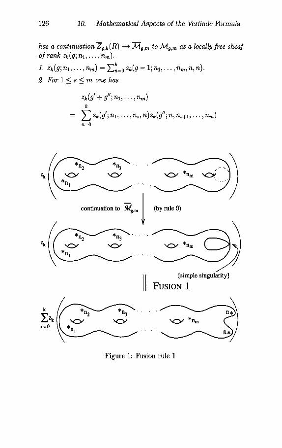
126 10. M a t h e m a t i c a l A s p e c t s of t h e V e r l i n d e F o r m u l a
has a c o n t i n u a t i o n - 2 g , k ( R ) ~ .Mg,m to A/lg,m as a locally f ree s h e a f
o f r a n k zk(g; nx, . . . , n m ) .
1. zk (g; n l , . . rim) k • , = ~ ,~=0 z k ( g -- 1; n l , . . . , rim, n, n).
2. F o r l < s < m one has
Zk(g' + g"; n l , . . . , rim)
k = ~ - ~ z k ( g ' ; n l , . . . , r l , s , n ) z k (g" ;n , rl, s+l , . . . , r~m)
n = 0
zk
m
continuation to ~,m (by rule O)
° , , , .
zk
[simple singularity]
FUSION 1
k ° °
Figure 1" Fusion rule 1
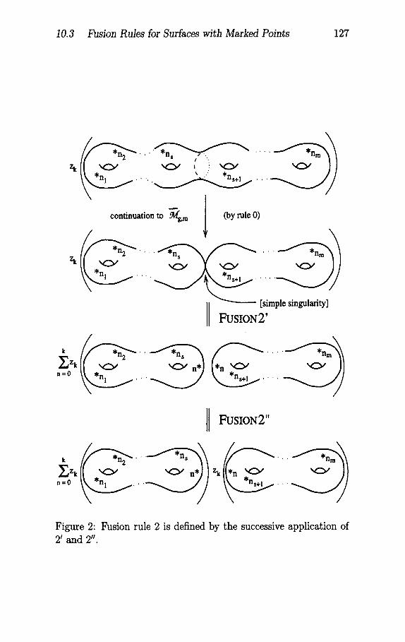
10.3 b-hsion Rules for Surfaces with Marked Points 127
2 ' '" ~'s t" ~ . . ~ . * n s + l . . . " . ~
continuation to -~,m (by role O)
~ ~ ' ' '. ~ ~ _ _ _ _ ~ ['i.'l. 'topic singularity]
° °
•=•0Zk ~ 2 '" , n ~ ' ~ '
1 FUSION2'
] FUSION2"
,:, ~ ~ z~(...~~ ' "~~~k
Figure 2" Fusion rule 2 is defined by the successive application of 2' and 2".
128 10. Mathematical Aspects of the Verlinde Formula
The formulation of the fusion rules for SU(2) in Theorem 10.9 is special since every representation p of the group SU(2) is equivalent to its conjugate representation p*. For more general Lie groups G instead of SU(2), one of the two representations (n, n) in the fusion rules has to be replaced with its conjugate.
A proof of the fusion rules 1 and 2 in approximately this form can be found in [NR93] together with [Ram94].
Even in the case of P = 0 it is quite difficult to show that the dimen- sions of H ° (A/[ sU(*) £k g , ) do not depend on the complex structure J. This can be deduced from a stronger property which states that the spaces
as well as
su(~) £k) H ° M j ,
su( l (p, R) Z, k) H ° (.A,,~j,g
are essentially independent of the complex structure. This is in agreement with physical requirements since these spaces are con- sidered to be the result of a quantization which only depends on the topology of S or S \ P. For this reason the resulting quantum field theory is called a topological quantum field theory (cf. [Wit89]). In particular, the state spaces- more precisely their projectivations - should not depend on any metric or complex structure.
That the above state spaces do not depend on the complex struc- ture has been proven in [APW91] and [Hit90] in the case of P = q}. Hitchin's methods carry over to the case of P ~ 0 using some re- sults of non-abelian Hodge theory [Sch92], [ScSc95]. The strategy of the proof is to consider the bundle Zg,k(R) ~ AzIg,m over the moduli space Azlg,m of Riemann surfaces of genus g and m marked
points with fiber H ° (^Asu(~)(p, R) £k v-,g,j , ) over (J, P) e AzIg,m. On this bundle Zg,k(R) one constructs a natural projectively flat con- nection. Incidentally, the existence of such a natural projectively flat connection is again motivated by considerations from conformal field theory. Then the fibers of the bundle can be identified in a natural way by parallel transport with respect to this connection up to a constant, i.e. they are projectively identified. It is remarkable that in the course of the construction in the general case of P ~ q} it seems to be necessary to use the metaplectic correction instead of the uncorrected geometric quantization (see [ScSc95]).
The case P ~ 0 is significant for the program of Witten, to describe the Jones polynomials of knot theory in the context of quantum
10.4 Combinatorics on Fusion Rings 129
field theory. In this picture, the Zk,g(R) are quantum mechanical state spaces, which can be found by path integration [Wit89] or by geometric quantization [Sch92], [ScSc95]. To obtain the knot invari- ants, one needs, in addition to these state spaces, the corresponding state vectors ("propagators") describing the time development. On the mathematical level this means that one has to assign to a com- pact three-dimensional manifold M with boundary containing la- beled knots a state vector in the state space given by the boundary of M which is a surface with marked points. For instance, one has to assign to such a manifold M with knots K = (Ks, . . . , / (8) , labeled by SU(r)-representations and with the boundary OM = Sg U S'g,, a vector Zk ( M, K) in
Zk,g(R)* ® Zk,g,(R') ~- Hom (Zk,g(R), Zk,g,(R')) .
The points in Sg, S'g, and the labels R, R' are induced by the knots K1, . . . , Ks, which may run from boundary to boundary. Only the state spaces together with the state vectors yield a topologi- cal quantum field theory. A rigorous construction of these state vec tors - which are given by path integration in [Wit89] - is still not known. In the meantime, instead of Witten's original program, other slightly modified constructions of topological quantum field theories - in some cases by using quantum groups - have been pro- posed (cf. e.g. [Tur94]) and yield interesting invariants of knots and three manifolds.
10.4 Combinator ics on Fusion Rings
Using the fusion rules of Sect. 10.3, the proof of the Verlinde for- mula can be reduced to the determination of
n, m), z (O; n, m, l)
for n, m, l E {0 , . . . , k}. This combinatorical reduction has an al- gebraification, which also has a meaning for more general groups than SU(r ) ( c f . [Bea94a], [eea94b], [Sze95]).
Def in i t ion 10.10 Let F be a finite-dimensional complex vector space with an element i E F. For every g E No and vl, . . . , vm E F let
130 10. Mathematical Aspects of the Verlinde Formula
be given. (F, 1, Z) is a fusion ring if the following fusion rules hold:
(El) Z(g)l .... ,1 = 1,
(F2) Z(g),, .... ,~,, = Z(g)l,,~ .... ,~,, does not depend on the order of the V l ~ . . . ~ V m .
(F3) v ~ Z(0),~,...,,j,,,,j+~,...,,~ is C-linear.
(F4) (v, w)---. Z(O),,~ is not degenerated.
We use the notation
f v Z(O)v, (v, w) Z(O)~,~ ~(v, w, u) Z(O)~,~,~. Q ~ and
Let (bj), (b i) be a pair of bases with ~ = (bj, bi). Then, additionally, the following rules hold
(F5) Z(g),~,...,,,~ = E Z ( g - 1)b,,~,,~,...,,=, g >_ 1 (Fusion 1).
' ' = E Z(g),, ..,,.,.b,Z(g')~.¢~ .¢ (Fu- (F6) Z(g + g )~, .... ,,~,~;,...,~,~ ,. .... , sion 2).
One easily proves
L e m m a 10.11 The product v . w := ~ ~(v, w, bj)b j for v, w e F induces on F the structure of a commutative and associative com- plex algebra.
L e m m a 10.12 With a "= ~ bib i = ~ ~(bi, b i, bk)b k e F the ab- stract Verlinde formula holds:
P r o o f By induction on m we show
The case m - 1 is trivial. For m > 2 we have
Z(g)Vl,...,~)m --- 2 Z(O)vl,v2,bjZ(g)bJ,v3 ..... ~)m by (F6)
= . . . . .
= Z Z(g),(,~,,~,b~)~,,3,...,,,~ by (F3)
= . . . .
= . . . .
10.4 Combinatorics on Fusion Rings 131
by the induction hypothesis. This implies
Z(g)v = y~ Z(g- 1)b~,~,v = Z(g- 1)av = Z(g- 2)~2v = Z(O)~gv.
Hence for v - vl . . . . . v m the claimed statement follows, m
For the derivation of the Verlinde formula (Theorem 10.6) from the fusion rules using Lemma 10.12 we refer to [Sze95], for example.
References
[APWgl] S. Axelrod, S. Della Pietra, and E. Witten. Geomet- ric quantization of Chern-Simons gauge theory. J. Diff. Geom. 33 (1991), 787-902.
[Bar54] V. Bargmann. On unitary ray representations of contin- uous groups. Ann. Math 59 (1954), 1-46.
[Bar64] V. Bargmann. Note on Wigner's theorem on symmetry operations. J. Math. Phys. 5 (1964), 862-868.
[BR77] A.O. Barut and R. Raczka. Theory of group represen- tations and applications. PWN - Polish Scientific Pub- lishers, 1977.
[Bea94a] A. Beauville. Conformal blocks, fusion rules and the Verlinde formula. Preprint, 1994.
[Bea94b] A. Beauville. Vector bundles on curves and general- ized theta functions: Recent results and open problems. Preprint, 1994.
[Bot91] R. Bott. Stable bundles revisited. Surveys in Differential Geometry (Supplement to J. Diff. Geom.)1 (1991), 1- 18.
[BPZ84] A.A. Belavin, A.M. Polyakov, and A.B. Zamolodchikov. Infinite conformal symmetry in two-dimensional quan- tum field theory. Nucl. Phys. B 241 (1984), 333-380.
[BT93]
[CdG94]
M. Blau and G. Thompson. Derivation of the Verlinde formula from Chern-Simons theory. Nucl. Phys. B 408 (1993), 345-390.
F. Constantinescu and H.F. de Groote. Geometrische und Algebraische Methoden der Physik: Supermannig- faltigkeiten und Virasoro-Algebren. Teubner, Stuttgart, 1994.
[Dic89]
[Die69]
R. Dick. Conformal Gauge Fixing in Minkowski Space. Letters in Mathematical Physics 18 (1989), 67-76.
J. Dieudonn6. Foundations of Modern Analysis, Volume 10-I. Academic Press, New York-London, 1969.
REFERENCES 133
[DFN84]
[Fa1941
[FFK89]
[FQS84]
[FQS86]
[FS87]
[Fuc92]
[Gaw89]
[GF68]
[Gin89]
[GKO86]
B.A. Dubrovin, A.T. Fomenko and S.P. Novikov. Modern geometry-methods and applications I. Springer-Verlag, 1984.
G. Faltings. A proof of the Verlinde formula. Geom. 3 (1994), 347-374.
J. Alg.
G. Felder, J. FrShlich, and J. Keller. On the structure of unitary conformal field theory, I. Existence of conformal blocks. Comm. Math. Phys. 124 (1989), 417-463.
D. Friedan, Z. Qiu, and S. Shenker. Conformal invari- ance, unitarity and two dimensional critical exponents. In Vertex operators in Mathematics and Physics, Eds. Lepowsky et al., pages 419-449. Springer Verlag, 1984.
D. Friedan, Z. Qiu, and S. Shenker. Details of the non- unitary proof for highest weight representations of the Virasoro algebra. Comm. Math. Phys. 107 (1986), 535- 542.
D. Friedan and S. Shenker. The analytic geometry of two-dimensional conformal field theory. Nucl. Phys. B 281 (1987), 509-545.
M. Fuchs. A]fine Lie Algebras and Quantum Groups. Cambridge University Press, 1992.
K. Gawedski. Conformal field theory. Sdm. Bourbaki 1988-89, AstGrisque 177-178 (no 704), 95-126, 1989.
I.M. Gelfand and D.B. Fuks. Cohomology of the Lie algebra of vector fields of a circle. Funct. Anal. Appl. 2 (1968), 342-343.
P. Ginsparg. Introduction to conformal field theory. Fields, Strings and Critical Phenomena, Les Houches 1988, Elsevier, Amsterdam 1989.
P. Goddard, A. Kent, and D. Olive. Unitary repre- sentations of the Virasoro and Super-Virasoro algebras. Comm. Math. Phys. 103 (1986), 105-119.
134 REFERENCES
[GO89]
[GSW87]
[Gw85]
[HS66]
[Hit90]
[Her71]
[HN91]
[IZ80]
[Kac80] •
[Kac90]
[KR87]
[Kak91]
[Kir76]
P. Goddard and D. Olive. Kac-Moody and Virasoro al- gebras in relation to quantum mechanics. Int. J. Mod. Physics A1 (1989), 303-414.
M.B. Green, J.H. Schwarz, and E. Witten. Superstring Theory, Vol. 1. Cambridge University Press, Cambridge, 1987.
R. Goodman and N.R. Wallach. Projective unitary positive-energy representations of Diff(S). Funct. Anal- ysis 63 (1985), 299-321.
N.S. Hawley and M. Schiffer. Half-order differentials on Riemann surfaces. Acta Math. 115 (1966), 175-236.
N. Hitchin. Flat connections and geometric quantization. Comm. Math. Phys. 131 (1990), 347-380.
M.-R. Herman. Simplicit~ du groupe des diff~omorphis- rues de classe C °°, isotope ~ l'identit~, du tore de dimen- sion n. C.R. Acad. Sci. Paris 273 (1971), 232-234.
J. Hilgert and K.-H. Neeb. bren. Vieweg, 1991.
Lie Gruppen und Lie Alge-
C. Itzykson and J.-B. Zuber. McGraw-Hill, 1980.
Quantum Field Theory.
V. Kac. Highest weight representations of infinite dimen- sional Lie algebras. In Proc. Intern. Congress Helsinki, Acad. Sci. Fenn., pages 299-304, 1980.
V. Kac. Infinite dimensional Lie algebras. Cambridge University Press, 3 rd ed., 1990.
V. Kac and A.K. Raina. Highest Weight Representations of Infinite Dimensional Lie Algebras. World Scientific, Singapore, 1987.
M. Kaku. Strings, Springer Verlag, 1991.
Conformal Fields and Topology.
A.A. Kirillov. Theory of Representations. Springer Ver- lag, 1976.
REFERENCES 135
[KJ88] A.A. Kirillov and D.V. Juriev. Representations of the Virasoro algebra by the orbit method. J. Geom. Phys. 5 (1988), 351-363.
[KNR94] S. Kumar, M.S. Narasimhan, and Ramanathan. Infinite Grassmanians and moduli spaces of G-bundles. Math. Ann. 300 (1994), 41-75.
[LM76] M. Liischer and G. Mack. The energy-momentum ten- sor of critical quantum field theory in 1+1 dimensions. Unpublished Manuscript, 1976.
[LPSA94] R. Langlands, P. Pouliot, and Y. Saint-Aubin. Confor- malinvariance in two-dimensional percolation. Bull. Am. Math. Soc. 30 (1994), 1-61.
[Mi184] J. Milnor. Remarks on infinite-dimensional Lie groups. In Relativity, Groups and Topology II, Les Houches 1983, pages 1007-1058. North-Holland, 1984.
[MS80] V. Mehta and C. Seshadri. Moduli of vector bundles on curves with parabolic structures. Ann. Math. 248 (1980), 205-239.
[MS891 G. Moore and N. Seiberg. Classical and conformal field theory. Comm. Math. Phys. 123 (1989), 177-254.
[MZ551 D. Montgomory and L. Zippin. Topological transforma- tion Groups. Interscience, New York, 1955.
[Nas91] C. Nash. Differential Topology and Quantum Field The- ory. Academic Press, 1991.
[NR93] M.S. Narasimhan and T. Ramadas. Factorization of gen- eralized theta functions I. Invent. Math. 114 (1993), 565-623.
INS65] M.S. Narasimhan and C. Seshadri. Stable and unitary vector bundles on a compact Riemann surface. Ann. Math. 65 (1965), 540-567.
[os73] K. Osterwalder and R. Schrader. Axioms for Euclidean Green's functions I. Comm. Math. Phys 31 (1973), 83- 112.
136 REFERENCES
[os75]
[Ram94]
[Sch92]
[ScSc95]
[Sch95]
[Seg88a]
[Seg88b]
[Seg91]
[Sire68]
[Sor95]
[Sze95]
[Tho84]
K. Osterwalder and R. Schrader. Axioms for Euclidean Green's functions II. Comm. Math. Phys 42 (1975), 281- 305.
T. Ramadas. Factorization of generalized theta functions II: The Verlinde formula. Preprint, 1994.
P. Scheinost. Metaplectic quantization of the moduli spaces of flat and parabolic bundles. Dissertation, LMU Miinchen, 1992.
P. Scheinost and M. Schottenloher. Metaplectic quanti- zation of the moduli spaces of flat and parabolic bundles. J. reine angew. Math. 466 (1995), 145-219.
M. Schottenloher. Geometrie und Symmetrie in der Physik. Vieweg, 1995.
G. Segal. The definition of conformal field theory. Un- published Manuscript, 1988.
G. Segal. Two dimensional conformal field theories and modular functors. In Proc. IXth Intern. Congress Math. Phys. Swansea, pages 22-37, 1988.
G. Segal. Geometric aspects of quantum field theory. Proc. Intern. Congress Kyoto 1990, Math. Soc. Japan, pages 1387-1396, 1991.
D. Simms. Lie Groups and Quantum Mechanics, Lecture Notes in Math. 52, Springer Verlag, 1968.
C. Sorger. La formule de Verlinde. Preprint, 1995. (to appear in Sem. Bourbaki, annie 1994-95, n ° 793)
A. Szenes. The combinatorics of the Verlinde formula. In Vector Bundles in Algebraic Geometry, Eds. Hitchin et al., pages 241-254. Cambridge Univ. Press, 1995.
C.B. Thorn. A proof of the no-ghost theorem using the Kac determinant. In Vertex operators in Mathemat- ics and Physics, Eds. Lepowsky et al., pages 411-417. Springer Verlag, 1984.
REFERENCES 137
[TUY89]
[Wu 94]
[Uen95]
[Ver88]
[Wig31]
[Wit89]
[Woo8O]
A. Tsuchiya, K. Ueno, and Y. Yamada. Conformal field theory on the universal family of stable curves with gauge symmetry, in: Conformal field theory and solv- able lattice models. Adv. Stud. Pure Math. 16 (1989), 297-372.
V.G. Turaev. Quantum invariants of knots and 3- manifolds. DeGruyter, 1994.
K. Ueno. On conformal field theory. In Vector Bundles in Algebraic Geometry, Eds. Hitchin et al., pages 283-345. Cambridge Univ. Press, 1995.
E. Verlinde. Fusion rules and modular transformations in two-dimensional conformal field theory. Nucl. Phys. B 300 (1988), 360-376.
E. Wigner. Gruppentheorie. Vieweg, 1931.
E. Witten. Quantum field theory and the Jones polyno- mial. Commun. Math. Phys. 121 (1989), 351-399.
N. Woodhouse. Geometric Quantization. Clarendon Press, 1980.
I n d e x
n-point function, 95 p-sphere, 4
abelian Lie algebra, 47 action, 78 adjoint action, 116 adjoint orbit, 121 angle preserving, 6, 7 anti-holomorphic
block, 107 function, 6, 16, 59 operator, 103 vector field, 60
anti-unitary operator, 38
biholomorphic, 7, 29, 31, 77 braid group, 96
canonical bundle, 119, 120 canonical quantization, 87 Casorati-Weierstra~, 31 Cech cohomology, 111 center of mass, 85 central charge, 103, 107 central extension, 56
of a Lie algebra, 47 of a group, 36
Chern-Simons theory, 111, 113 coadjoint action, 116 coadjoint orbit, 116, 121 cohomology
group, 46, 51 of groups, 46, 111 of Lie algebras, 51
commutation relations, 67, 69- 71, 88, 93, 103, 104
commutator, 57, 87 complex structure, 107, 112,
114, 116-119, 121,128
complexification, 32, 35, 57, 116 conformal, 5, 6, 16
group, 58, 83 weight, 98 block, 107, 110, 117, 119 compactification, 22, 35 continuation, 23 diffeomorphism, 9, 20, 23,
33, 35 factor, 5, 8 family, 106 field theory, 30, 32, 58, 59,
65, 76, 78, 86, 95, 101, 107, 108, 117, 128
gauge, 83 group, 20, 24, 29, 31, 32,
35, 56 Killing factor, 11, 12, 14,
16, 19, 28 Killing field, 10-17, 19, 32 spin, 98 structure, 22, 35 symmetry, 35, 46, 58, 102,
104, 107 symmetry algebra, 59 transformation, 5, 12-17,
19, 20, 23, 24, 26-30, 33, 59, 83, 97
weight, 103 conformally fiat, 80 conjugacy classes, 121 connection, 113 constraints, 32, 60, 83 correlation function, 95, 96, 98,
109 covariance, 98 covariant derivative, 11 covering, 22
INDEX 139
curvature, 114, 123 cyclic, 66
decomposable, 74 Deligne-Mumford compactifi-
cation, 125 descendant, 106, 108 determinant bundle, 113, 125 differentiable structure, 47, 54 dilatation, 14, 16, 17, 26, 97,
101 distribution, 95
energy-momentum tensor, 80, 84, 86, 101, 103, 105
equations of motion, 86 equivalence of extensions, 43,
48 Euclidean
group, 97 motion, 17, 97 plane, 4, 7, 16, 31, 32, 58 quantum field theory, 95 signature, 58, 95 structure, 6
exact sequence, 36, 43, 44, 47, 48, 52
extension of a Lie algebra, 47 of a group, 36
field operator, 60, 95, 100, 101 flag, 116, 123 flat SU(r)-bundles, 111 flat connection, 111 flat vector bundle, 111 flow equation, 10 Fock space, 88, 90, 93 Fourier series, 57, 83, 85 Fr~chet space, 40, 56 fundamental group, 96, 111,121 fusion ring, 130
fusion rules, 107, 119, 125, 128- 131
Galilei group, 39 gauge, 111 gauge group, 39, 111, 113 generalized
theta functions, 125 geometric quantization, 114, 116,
119, 128, 129 global conformal transforma-
tion, 28 Green's function, 95 group of motions, 14
hermitian form, 65, 69-71, 73, 74, 88, 93, 94, 96, 100
highest weight, 66, 92, 93 representation, 66, 70, 74,
75, 106 vector, 66, 70, 75, 92, 106
Hilbert space, 37, 66, 95, 96, 100
holomorphic block, 107 continuation, 28 function, 6, 16, 17, 28-31,
59, 102 line bundle, 114, 117, 124 operator, 97, 101, 103 polarization, 114, 115 section, 107, 114 transformation, 59 vector bundle, 112, 114, 117,
123 vector field, 59
holonomy, 122 homogeneous coordinates, 21 homology group, 111
indecomposable, 74, 75 induced representation, 68
140 INDEX
invariant linear subspace, 69 inversion, 17, 97 irreducible, 75, 88, 117, 121 isometry, 5, 9, 13, 14, 17, 22,
29 isothermal coordinates, 80, 81,
83, 85, 86 isotropy group, 116
Jacobi variety, 117 Jones polynomial, 128
K~ihler manifold, 112, 116, 119 Kac determinant, 72, 74, 94 Kac-Moody algebra, 74, 76, 108 Killing field, 13 knot theory, 128
label, 121, 124 Laplace-Beltrami operator, 11 Laurent series, 59 level, 125 Levi-Civita connection, 11 Lie Mgebra, 13, 15, 31, 32i 35,
47-49, 52, 56, 58, 59, 65, 76, 88, 123
of vector fields, 57 Lie bracket, 15, 32, 47, 49, 50,
57-60, 88 Lie derivative, 11 Lie group, 14, 31, 40, 47-49,
51, 52, 55, 56, 60, 76, 105, 112, 117, 118
lift, 51, 53, 55, 76 local one-parameter group, 10 locality, 97 Lorentz group, 29, 55 Lorentz manifold, 78, 80 Lorentz metric, 78, 81
MSbius group, 31, 97 MSbius transformation, 17, 29,
31, 97
marked point, 121, 122, 128 Marsden-Weinstein reduction,
113, 123 matrix coefficients, 95 meromorphic, 114 metaplectic quantization, 119,
128 Minkowski plane, 4, 9, 32, 35 Minkowski space, 4 moduli space, 107, 112, 117,
121, 124, 125, 128 of parabolic bundles, 122 of representations, 110 of vector bundles, 112
moment map, 113 monomials, 88
Nambu-Goto action, 78 no-ghost theorem, 94 non-abelian Hodge theory, 128 normal ordering, 89, 90, 104
one-parameter group, 10, 13, 15-17, 19
OPE, 105, 106 operator product expansion, 101,
104-106 orbifold fundamental group, 122 orientation preserving, 5 orientation-preserving, 7, 16,
18, 19, 28, 29, 33, 35 orthogonal transformation, 13,
15, 24 oscillator, 119 oscillator algebra, 88 oscillator modes, 85 Osterwalder-Schrader Axioms,
97
parabolic structure, 123 paradegree, 124 paradeterminant, 124
INDEX 141
parallel transport, 128 phase space, 37, 111, 113-115,
122 Poincar~ group, 39, 97 Poincar~ transformation, 80 Poisson bracket, 87 polarization, 114, 115 Polyakov action, 79 polynomial vector fields, 58 prequantum bundle, 114-117 preserve angles infinitesimally,
7 primary field, 60, 101,104-107,
119 projective automorphisms, 38 projective representation, 51,
56, 66, 76, 77 projective space, 20, 37 projectively flat connection, 128
quadric, 4, 21 quantization, 40, 87, 93
of symmetries, 37, 39, 40, 43, 56
quantum field theory, 95 quantum group, 129
radial quantization, 96, 101,108 rational conformal field theory,
108, 119 reconstruction of the field op-
erator, 100 reducible, 75 reflection positivity, 96, 99 removable singularity theorem,
31 reparameterization, 80 Riemann sphere, 29 Riemann surface, 77, 95, 107,
109, 112, 117, 123, 125 Riemann zeta function, 61 Riemannian manifold, 4
rotation, 97
scaling covariance, 99, 101 scaling dimension, 98 Schwartz space, 96 secondary field, 106 self-adjoint operator, 55, 76,
95, 101, 115 semi-direct product, 7, 14 semi-Riemannian manifold, 3,
4, 12, 78 semi-simple Lie algebra, 55 semi-stable, 124 sheaf, 114 shift by the dual Coxeter num-
ber, 119-121 simple Lie group, 118, 121 simply connected universal cov-
ering, 41 singular connection, 123 special conformal transforma-
tion, 15, 16, 26 splitting of an exact sequence
of groups, 43 of Lie Algebras, 48
stable, 124 state space, 37, 115, 128 stereographic projection, 8 string, 78, 83, 85 string algebra, 93 string theory, 32, 73, 78, 93,
108 strong topology, 40, 41 submodule, 69-71 symmetry group, 83 symplectic form, 40, 113, 116 symplectic manifold, 112, 114 symplectic structure, 112, 113
theta bundle, 117, 125 theta divisor, 117 theta functions, 110, 117
142 INDEX
generalized, 110, 114, 117 time reflection, 97 time-ordered product, 95 topological group, 40 topological quantum field the-
ory, 128, 129 transition probability, 37 translation, 13, 15, 25, 97, 98,
102 trivial extension
of a group, 36 of a Lie algebra, 48
unitary, 72-74, 93, 94, 103 group, 37 highest weight representa-
tion, 74, 75, 92, 93, 104, 108
operator, 37, 38 representation, 51, 55, 56,
65, 66, 69, 74, 76, 77, 88, 104, 105, 117
universal covering, 96 universal covering group, 41,
42, 55 universal enveloping algebra, 68
vacuum, 91 vacuum expectation value, 95 vacuum vector, 66, 74, 88, 108 vector bundle, 111 Verlinde formula, 110, 118, 119,
129-131 Verma module, 66, 67, 69, 70,
75, 93 Virasoro algebra, 35, 48, 56,
60, 64, 69, 90, 92, 103 Virasoro module, 66, 68-71,108
wave equation, 19, 34, 83, 85 weights, 124 Weyl rescaling, 80
Witt algebra, 32, 35, 48, 56, 58-60, 64
world sheet, 78, 83
Lecture Notes in Physics For information about Vols. 1-449 please contact your bookseller or Springer-Verlag
Vol. 450: M. F. Shlesinger, G. M. Zaslavsky, U. Frisch (Eds.), L~vy Flights and Related Topics in Physics. Proceedigs, 1994. XIV, 347 pages. 1995.
Vol. 451: P. Kr~e, W. Wedig (Eds.), Probabilistic Methods in Applied Physics. IX, 393 pages. 1995.
Vol. 452: A. M. Bernstein, B. R. Holstein (Eds.), Chiral Dynamics: Theory and Experiment. Proceedings, 1994. VIII, 351 pages. 1995.
Vol. 453: S. M. Deshpande, S. S. Desai, R. Narasimha (Eds.), Fourteenth International Conference on Numerical Methods in Fluid Dynamics. Proceedings, 1994. XIII, 589 pages. 1995.
Vol. 454: ]. Greiner, H. W. Duerbeck, R. E. Gershberg (Eds.), Flares and Flashes, Germany 1994. XXII, 477 pages. 1995.
Vol. 455: F. Occhionero (Ed.), Birth of the Universe and Fundamental Physics. Proceedings, 1994. XV, 387 pages. 1995.
Vol. 456: H. B. Geyer (Ed.), Field Theory, Topology and Condensed Matter Physics. Proceedings, 1994. XII, 2o6 pages. 1995.
Vol. 457: P. Garbaczewski, M. Wolf, A. Weron (Eds.), Chaos - The Interplay Between Stochastic and De- terministic Behaviour. Proceedings, 1995. XII, 573 pages. 1995.
Vol. 458: I. W. Roxburgh, ].-L. Masnou (Eds.), Physical Processes in Astrophysics. Proceedings, 1993. XII, 249 pages. 1995.
Vol. 459: G. Winnewisser, G. C. Pelz (Eds.), The Physics and Chemistry of Interstellar Molecular Clouds. Proceedings, 1993. XV, 393 pages. 1995.
Vol. 46o: S. Cotsakis, G. W. Gibbons (Eds.), Global Structure and Evolution in General Relativity. Pro- ceedings, 1994. IX, 173 pages. 1996.
Vol. 461: R. L6pez-Pen'a, R. Capovilla, R. Garcl'a-Pelayo, H. Waelbroeck, F. Zertuche (Eds.), Complex Systems and Binary Networks. Lectures, M~xico 1995. X, 223 pages. 1995.
Vol. 462: M. Meneguzzi, A. Pouquet, P.-L. Sulem (Eds.), Small-Scale Structures in Three-Dimensional Hydro- dynamic and Magnetohydrodynamic Turbulence. Pro- ceedings, 1995. IX, 421 pages. 1995.
Vol. 463: H. Hippelein, K. Meisenheimer, H.-]. R6ser (Eds.), Galaxies in the Young Universe. Proceedings, 1994. XV, 314 pages. 1995.
Vol. 464: L. Ratke, H. U. Walter, B. Feuerbach (Eds.), Materials and Fluids Under Low Gravity. Proceedings, 1994. XVIII, 424 pages, 1996.
Vol. 465: S. Beckwith, J. Staude, A. Quetz, A. Natta (Eds.), Disks and Outflows Around Young Stars. Proceedings, 1994. XII, 361 pages, 1996.
Vol. 466: H. Ebert, G. Schtitz (Eds.), Spin - Orbit-In- fluenced Spectroscopies of Magnetic Solids. Proceedings, 1995. VII, 287 pages, 1996.
Vol. 467: A. Steinchen (Ed.), Dynamics of Multiphase Flows Across Interfaces. 1994/1995. XII, 267 pages. 1996.
Vol. 468: C. Chiuderi, G. Einaudi (Eds.), Plasma Astro- physics. 1994. VII, 326 pages. 1996.
Vol. 469: H. Grosse, L. Pittner (Eds.), Low-Dimensional Models in Statistical Physics and Quantum Field Theory. Proceedings, 1995. XVII, 339 pages. 1996.
Vol. 470: E. Martl'nez-Gonz~tlez, ]. L. Sanz (Eds.), The Universe at High-z, Large-Scale Structure and the Cosmic Microwave Background. Proceedings, 1995. VIII, 254 pages. 1996.
Vol. 471: W. Kundt (Ed.), lets from Stars and Galactic Nuclei. Proceedings, 1995. X, 29o pages. 1996.
Vol. 472: ]. Greiner (Ed.), Supersoft X-Ray Sources. Proceedings, 1996. XIII, 35o pages. 1996.
Vol. 473: P. Weingartner, G. Schurz (Eds.), Law and Prediction in the Light of Chaos Research. X, 291 pages. 1996.
Vol. 474: Aa. Sandqvist, P. O. Lindblad (Eds.), Barred Galaxies and Circumnuclear Activity. Proceedings of the Nobel Symposium 98,1995. XI, 306 pages. 1996.
Vol. 475: J. Klamut, B. W. Veal, B. M. Dabrowski, P. W. Klamut, M. Kazimierski (Eds.), Recent Developments in High Temperature Superconductivity. Proceedings, 1995. XIII, 362 pages. 1996.
Vol. 476: ]. Parisi, S. C. Mtiller, W. Zimmermann (Eds.), Nonlinear Physics of Complex Systems. Current Status and Future Trends. XIII, 388 pages. 1996.
Vol. 477: Z. Petru, ]. Przystawa, K. Rapcewicz (Eds.), From Quantum Mechanics to Technology. Proceedings, 1996. IX, 379 pages. 1996.
Vol. 479: H. Latal, W. Schweiger (Eds.), Perturbative and Nonperturbative Aspects of Quantum Field Theory. Proceedings, 1996. X, 430 pages. 1997.
Vol. 480: H. Flyvbjerg, J. Hertz, M. H. ]ensen, O. G. Mouritsen, K. Sneppen (Eds.), Physics of Biological Sys- tems. From Molecules to Species. X, 364 pages. 1997.
New Series m: Monographs
Vol. m 1: H. Hora, Plasmas at High Temperature and Density. VIII, 442 pages. 1991.
Vol. m 2: P. Busch, P. J. Lahti, P. Mittelstaedt, The Quan- tum Theory of Measurement. XIII, 165 pages. 1991. Second Revised Edition: XIII, 181 pages. 1996.
Vol. m 3: A. Heck, J. M. Perdang (Eds.), Applying Fractals in Astronomy. IX, 21o pages. 1991.
Vol. m 4: R. K. Zeytounian, M&anique des fluides fonda- mentale. XV, 615 pages, 1991.
Vol. m 5: R. K. Zeytounian, Meteorological Fluid Dynamics. XI, 346 pages. 1991.
Vol. m 6: N. M. J.Woodhouse, Special Relativity. VIII, 86 pages. 1992.
Vol. m 7: G. Morandi, The Role of Topology in Classical and Quantum Physics. XIII, 239 pages. 1992.
Vol. m 8: D. Funaro, Polynomial Approximation of Dif- ferential Equations. X, 305 pages. 1992.
Vol. m 9: M. Namiki, Stochastic Quantization. x, 217 pages. 1992.
Vol. m lO: J. Hoppe, Lectures on Integrable Systems. VII, 111 pages. 1992.
Vol. m 11: A. D. Yaghjian, Relativistic Dynamics of a Charged Sphere. XII, 115 pages. 1992.
V o l . m 12: G. Esposito, Quantum Gravity, Quantum Cosmology and Lorentzian Geometries. Second Corrected and Enlarged Edition. XVIII, 349 pages. 1994.
Vol. m 13: M. Klein, A. Knauf, Classical Planar Scattering by Coulombic Potentials. V, 142 pages. 1992.
Vol. m 14: A. Lerda, Anyons. XI, 138 pages. 1992.
Vol . m 15: N. Peters, B. Rogg (Eds.), Reduced Kinetic Mechanisms for Applications in Combustion Systems. X, 36o pages. 1993.
Vol. m 16: P. Christe, M. Henkel, Introduction to Conformal Invariance and Its Applications to Critical Phenomena. XV, 260 pages. 1993.
Vol. m 17: M. Schoen, Computer Simulation of Condensed Phases in Complex Geometries. X, 136 pages. 1993.
Vol. m 18: H. Carmichael, An Open Systems Approach to Quantum Optics. X, 179 pages. 1993.
Vol. m 19: S. D. Bogan, M. K. Hinders, Interface Effects in Elastic Wave Scattering. XII, 182 pages. 1994.
Vol . m 2o: E. Abdalla, M. C. B. Abdalla, D. Dalmazi, A. Zadra, 2D-Gravity in Non-Critical Strings. IX, 319 pages. 1994.
Vol . m 21: G. P. Berman, E. N. Bulgakov, D. D. Holm, Crossover-Time in Quantum Boson and Spin Systems. XI, 268 pages. 1994.
Vol. m 22: M.-O. Hongler, Chaotic and Stochastic Behaviour in Automatic Production Lines. V, 85 pages. 1994.
Vol. m 23: V. S. Viswanath, G. Mtiller, The Recursion Method. X, 259 pages. 1994.
Vol. m 24: A. Ern, V. Giovangigli, Multicomponent Trans- port Algorithms. XIV, 427 pages. 1994.
Vol. m 25: A. V. Bogdanov, G. V. Dubrovskiy, M. P. Krutikov, D. V. Kulginov, V. M. Strelchenya, Interaction of Gases with Surfaces. XIV, 132 pages. 1995.
Vol. m 26: M. Dineykhan, G. V. Efimov, G. Ganbold, S. N. Nedelko, Oscillator Representation in Quantum Physics. IX, 279 pages. 1995.
Vol. m 27: J. T. Ottesen, Infinite Dimensional Groups and Algebras in Quantum Physics. IX, 218 pages. 1995.
Vol. m 28: O. Piguet, S. P. Sorella, Algebraic Renormal- ization. IX, 134 pages. 1995.
Vol. m 29: C. Bendjaballah, Introduction to Photon Communication. VII, 193 pages. 1995.
Vol. m 3o: A. J. Greet, W. J. Kossler, Low Magnetic Fields in Anisotropic Superconductors. VII, 161 pages. 1995.
Vol. m 31: P. Busch, M. Grabowski, P. J. Lahti, Operational Quantum Physics. XI, 23o pages. 1995.
Vol. m 3z: L. de Broglie, Diverses questions de m&anique et de thermodynamique classiques et relativistes. XII, 198 pages. 1995.
Vol. m 33: R. Alkofer, H. Reinhardt, Chiral Quark Dynamics. VIII, 115 pages. 1995.
Vol. m 34: R. Jost, Das M~irchen vom Elfenbeinernen Turm. VIII, 286 pages. 1995.
Vol. m 35: E. Elizalde, Ten Physical Applications of Spec- tral Zeta Functions. XIV, 228 pages. 1995.
Vol. m 36: G. Dunne, Self-Dual Chern-Simons Theories. X, 217 pages. 1995.
Vol. m 37: S. Childress, A.D. Gilbert, Stretch, Twist, Fold: The Fast Dynamo. XI, 41o pages. 1995.
Vol. m 38: J. Gonz~lez, M. A. Martin-Delgado, G. Sierra, A. H. Vozmediano, Quantum Electron Liquids and High-Tc Superconductivity. X, 299 pages. 1995.
Vol. m 39: L. Pittner, Algebraic Foundations of Non-Com- mutative Differential Geometry and Quantum Groups. XII, 469 pages. 1996.
Vol. m 4o: H.-J. Botchers, Translation Group and Particle Representations in Quantum Field Theory. VII, 131 pages. 1996.
Vol. m 41: B. K. Chakrabarti, A. Dutta, P. Sen, Quantum Ising Phases and Transitions in Transverse Ising Models. X, 2o4 pages. 1996.
Vol. m 42: P. Bouwknegt, J. McCarthy, K. Pilch, The V03 Algebra. Modules, Semi-infinite Cohomology and BV Algebras. XI, 2o4 pages. 1996.
Vol. m 43: M. Schottenloher, A Mathematical Introduction to Conformal Field Theory. VIII, 142 pages. 1997.
Vol. m 44: A. Bach, Indistinguishable Classical Particles. VIII, 157 pages. 1997.
Vol. m 45: M. Ferrari, V. T. Granik, A. Imam, J. C. Nadeau (Eds.), Advances in Doublet Mechanics. XVI, 214 pages. 1997.
Related Documents


![[LNP] Durarara!! Gaiden 01](https://static.cupdf.com/doc/110x72/55cf991c550346d0339ba1eb/lnp-durarara-gaiden-01.jpg)