DISCRETE AND CONTINUOUS Website: http://AIMsciences.org DYNAMICAL SYSTEMS Volume 10, Number 3, April 2004 pp. 657–678 A CONSTRUCTIVE CONVERSE LYAPUNOV THEOREM ON EXPONENTIAL STABILITY Sigurdur Freyr Hafstein ∗ Department of Theoretical Physics Gerhard-Mercator-University, Duisburg, D-47057, Germany Abstract. Closed physical systems eventually come to rest, the reason being that due to friction of some kind they continuously lose energy. The mathematical exten- sion of this principle is the concept of a Lyapunov function. A Lyapunov function for a dynamical system, of which the dynamics are modelled by an ordinary differential equation (ODE), is a function that is decreasing along any trajectory of the system and with exactly one local minimum. This implies that the system must eventu- ally come to rest at this minimum. Although it has been known for over 50 years that the asymptotic stability of an ODE’s equilibrium is equivalent to the existence of a Lyapunov function for the ODE, there has been no constructive method for non-local Lyapunov functions, except in special cases. Recently, a novel method to construct Lyapunov functions for ODEs via linear programming was presented [5], [6], which includes an algorithmic description of how to derive a linear program for a continuous autonomous ODE, such that a Lyapunov function can be constructed from any feasible solution of this linear program. We will show how to choose the free parameters of this linear program, dependent on the ODE in question, so that it will have a feasible solution if the equilibrium at the origin is exponentially sta- ble. This leads to the first constructive converse Lyapunov theorem in the theory of dynamical systems/ODEs. 1. Introduction. The Lyapunov theory of dynamical systems is the most useful general theory for studying the stability of nonlinear systems. It is covered in practically all textbooks on dynamical systems, on control theory, and in many on ordinary differential equation. It was introduced by Alexandr M. Lyapunov in 1892 and includes two methods, Lyapunov’s indirect method and Lyapunov’s direct method. An English translation of his work can be found in [4] Lyapunov’s direct method is a mathematical extension of the fundamental phys- ical observation, that an energy dissipative system must eventually settle down to an equilibrium point. It states that if there is an energy-like function V for a system that is strictly decreasing along its trajectories, then the trajectories are asymptotically attracted to an equilibrium. The function V is then said to be a Lyapunov function for the system. The region (basin, domain) of attraction of a dynamical systems’ equilibrium is the set of those initial values that are attracted to the equilibrium by the dynamics of the system. A Lyapunov function provides through its preimages a lower bound of the region of attraction. This bound is non-conservative in the sense that it extends to the boundary of the domain of the Lyapunov function. 1991 Mathematics Subject Classification. 93D05, 93D20, 93D30, 34D05, 34D20. Key words and phrases. Lyapunov functions, converse theorems, dynamical systems, ordinary differential equations, linear programming, control theory, exponential stability. ∗ Former name ’SigurðurFreyrMarin´osson’. 657

Welcome message from author
This document is posted to help you gain knowledge. Please leave a comment to let me know what you think about it! Share it to your friends and learn new things together.
Transcript
DISCRETE AND CONTINUOUS Website: http://AIMsciences.orgDYNAMICAL SYSTEMSVolume 10, Number 3, April 2004 pp. 657–678
A CONSTRUCTIVE CONVERSE LYAPUNOV THEOREM ONEXPONENTIAL STABILITY
Sigurdur Freyr Hafstein ∗
Department of Theoretical PhysicsGerhard-Mercator-University, Duisburg, D-47057, Germany
Abstract. Closed physical systems eventually come to rest, the reason being thatdue to friction of some kind they continuously lose energy. The mathematical exten-sion of this principle is the concept of a Lyapunov function. A Lyapunov function fora dynamical system, of which the dynamics are modelled by an ordinary differentialequation (ODE), is a function that is decreasing along any trajectory of the systemand with exactly one local minimum. This implies that the system must eventu-ally come to rest at this minimum. Although it has been known for over 50 yearsthat the asymptotic stability of an ODE’s equilibrium is equivalent to the existenceof a Lyapunov function for the ODE, there has been no constructive method fornon-local Lyapunov functions, except in special cases. Recently, a novel method toconstruct Lyapunov functions for ODEs via linear programming was presented [5],[6], which includes an algorithmic description of how to derive a linear program fora continuous autonomous ODE, such that a Lyapunov function can be constructedfrom any feasible solution of this linear program. We will show how to choose thefree parameters of this linear program, dependent on the ODE in question, so thatit will have a feasible solution if the equilibrium at the origin is exponentially sta-ble. This leads to the first constructive converse Lyapunov theorem in the theory ofdynamical systems/ODEs.
1. Introduction. The Lyapunov theory of dynamical systems is the most usefulgeneral theory for studying the stability of nonlinear systems. It is covered inpractically all textbooks on dynamical systems, on control theory, and in manyon ordinary differential equation. It was introduced by Alexandr M. Lyapunov in1892 and includes two methods, Lyapunov’s indirect method and Lyapunov’s directmethod. An English translation of his work can be found in [4]
Lyapunov’s direct method is a mathematical extension of the fundamental phys-ical observation, that an energy dissipative system must eventually settle downto an equilibrium point. It states that if there is an energy-like function V for asystem that is strictly decreasing along its trajectories, then the trajectories areasymptotically attracted to an equilibrium. The function V is then said to be aLyapunov function for the system. The region (basin, domain) of attraction of adynamical systems’ equilibrium is the set of those initial values that are attractedto the equilibrium by the dynamics of the system. A Lyapunov function providesthrough its preimages a lower bound of the region of attraction. This bound isnon-conservative in the sense that it extends to the boundary of the domain of theLyapunov function.
1991 Mathematics Subject Classification. 93D05, 93D20, 93D30, 34D05, 34D20.Key words and phrases. Lyapunov functions, converse theorems, dynamical systems, ordinary
differential equations, linear programming, control theory, exponential stability.∗Former name ’Sigurður Freyr Marinosson’.
657
658 SIGURDUR FREYR HAFSTEIN
There are several possibilities to formulate Lyapunov’s direct method. In thiswork we follow [5] and only consider autonomous systems, where the dynamics ofthe system are modelled by an ODE
x = f(x), (1.1)
where f ∈ [C2(U)]n is a function from a domain U ⊂ Rn into R
n, of which everycomponent fi is two-times continuously differentiable, and such that 0 ∈ U andf(0) = 0. We denote by φ the solution of (1.1), i.e., φ(t, ξ) = f(φ(t, ξ)) andφ(0, ξ) = ξ for all ξ ∈ U and all (possible) t. In this case the direct method ofLyapunov states (proved in Chapter 1 in [5]):
Proposition 1.1. Consider the ODE (1.1) and assume there is a domain M inR
n, 0 ∈ M ⊂ U , and a locally Lipschitz and positive definite function V : M −→ R,i.e. V (0) = 0 and V (x) > 0 for all x ∈ M \ {0}, such that
lim sups→0+
V (φ(t, ξ) + sf(φ(t, ξ))) − V (φ(t, ξ))s
< 0
for all φ(t, ξ) ∈ M. Then every compact and connected component of every preim-age V −1([0, c]), c > 0, that contains the origin is a subset of the region of attraction
{ξ ∈ U∣∣ lim supt→+∞
φ(t, ξ) = 0}
of the equilibrium at the origin.
The function V in Proposition 1.1 is called a Lyapunov function for the ODE(1.1). For every ξ �= 0 in the domain of the Lyapunov function, the functiont �→ V (φ(t, ξ)) is strictly decreasing on its domain. This implies, that every solutionof (1.1) does either leave the boundary of the domain of the Lyapunov functionor it is asymptotically attracted to the origin. The latter is necessarily the caseif the initial value ξ is in a connected compact component of a set of the formV −1([0, c]), c > 0, that contains the origin, for else there would be a contradictionto t �→ V (φ(t, ξ)) being decreasing.
Proposition 1.1 is particularly useful when V ∈ C1(M) and f ∈ [C1(U)]n. Then
lim sups→0+
V (φ(t, ξ) + sf(φ(t, ξ))) − V (φ(t, ξ))s
= [∇V ](φ(t, ξ)) · f(φ(t, ξ))
by the chain rule and the right-hand side of this equation can be checked for nega-tivity without knowing the solution φ.
Although the direct method of Lyapunov is a powerful tool for stability analysis,its main drawback has been the lack of a general constructive method to generatenon-local Lyapunov functions for nonlinear ODEs. A local Lyapunov function canbe constructed if the Jacobian A ∈ R
n×n of f at the origin is Hurwitz, i.e., if allits eigenvalues have strictly negative real parts. Then, by the indirect method ofLyapunov, V (x) = xTPx is a Lyapunov function for the system, where P ∈ R
n×n
is the unique positive definite solution to the matrix equation †
PA+ATP = −In.However, the domain of this Lyapunov function depends on the approximation errorx �→ f(x) − Ax and, except when f is a linear function, almost certainly does notgive a good estimate of the region of attraction.
†AT and xT denote the transposes of the matrix A and the vector x respectively and In
denotes the n × n-identity matrix.
A CONSTRUCTIVE CONVERSE LYAPUNOV THEOREM 659
Let us make this point more clear. The function V (x) = xTPx is a globalLyapunov function for the linearized ODE x = Ax. This follows by V (0) = 0,V (0) > 0 for all x ∈ R
n \ {0}, and
d
dtV (φlin) = φT
linP φlin + φT
linPφlin
= φTlinPAφlin + φT
linATPφlin
= −‖φlin‖22 (< 0 for all φlin ∈ R
n \ {0}),where φlin is the solution of the linear ODE. From this it deduces that
d
dtV (φ) = −‖φ‖2
2 + φTP (f(φ) −Aφ) + (f(φ) −Aφ)TPφ
≤ −‖φ‖22 + 2‖φ‖2‖P‖2‖f(φ) −Aφ‖2
and because f is differentiable at the origin there is a neighborhood of the origin,such that
‖f(x) −Ax‖2 <‖x‖2
2‖P‖2, (1.2)
for all x in this neighborhood. By these calculations, V is a Lyapunov function forthe ODE (1.1) too. However, its domain is not only restricted by the equilibrium’sregion of attraction, but also to the neighborhood in which (1.2) is satisfied, thatcan be very small in comparison to the equilibrium’s region of attraction.
The original Lyapunov theory did not secure the existence of non-local Lyapunovfunctions for nonlinear systems with asymptotically stable equilibrium points. Thefirst results on this subject are due to K. P. Perdeskii in 1933 [2]. The general casewas resolved somewhat later. Theorems, which secure the existence of a Lyapunovor a Lyapunov-like function for a system possessing an equilibrium, stable in somesense, are called converse theorems in the theory of dynamical systems. Most of theconverse theorems are proved by actually constructing by a finite or a transfiniteprocedure a Lyapunov(-like) function. Unfortunately, the trajectories of the respec-tive systems are used by the construction methods. Hence, the converse theoremshave up-to-date been pure existence theorems.
In this work we will prove a constructive converse theorem on exponential sta-bility. The origin is said to be an exponentially stable equilibrium of (1.1), if andonly if there is a neighborhood N of the origin and constants α > 0 and m ≥ 1,such that ‖φ(t, ξ)‖2 ≤ me−αt‖ξ‖2 for all ξ ∈ N and all t ≥ 0. The concept of anexponentially stable equilibrium point is mathematically more restrictive than theconcept of an asymptotically stable equilibrium, where it is only demanded thatthere exists a neighborhood of the origin, such that all trajectories starting in thisneighborhood are attracted to the equilibrium by the dynamics of the system. Al-though asymptotically stable equilibrium points that are not exponentially stableare an interesting mathematical phenomena (bifurcations), most equilibrium pointsare either exponentially stable or not asymptotically stable. If the real parts of alleigenvalues of the Jacobian of f at the origin are strictly negative, then the originis exponentially stable, if one is strictly positive then it is unstable, and if all arenegative and some are equal to zero, then the origin might be asymptotically stablebut is not exponentially stable. In the last case the stability is usually not robustto perturbations and is therefore not desirable in engineering applications. A wellknown non-constructive converse theorem on exponential stability states:
660 SIGURDUR FREYR HAFSTEIN
Proposition 1.2. Assume there is an open neighborhood N ⊂ U of the ori-gin and constants α > 0 and m ≥ 1, such that the solution φ of (1.1) sat-isfies ‖φ(t, ξ)‖2 ≤ me−αt‖ξ‖2 for all ξ ∈ N and all t ≥ 0. Suppose the set{y ∈ R
n∣∣‖y‖2 ≤ m supz∈N ‖z‖2} is a compact subset of U and let L be a Lips-
chitz constant for f on this compact set. Let T be a constant satisfying
T >1α
ln(m).
Then the function W : N −→ R,
W (ξ) :=∫ T
0
‖φ(τ, ξ)‖22dτ
for all ξ ∈ N , satisfies the inequalities
1 − e−2LT
2L‖ξ‖2
2 ≤W (ξ) ≤ m2 1 − e−2αT
2α‖ξ‖2
2
and∇W (ξ) · f(ξ) ≤ −(1 −m2e−2αT )‖ξ‖2
2
for all ξ ∈ N , and is therefore a Lyapunov function for (1.1).
This converse theorem is useful because it gives an explicit formula for a Lya-punov function for the system. However, it is non-constructive because this formulainvolves the solution of the ODE, which, in general, is not known. We will use thisLyapunov function formula to prove that the linear program in the next section hasa feasible solution.
The Lyapunov theory is covered in numerous textbooks on dynamical systems,e.g., [3], [7], [2], [9]. In [5] Proposition 1.1 (Theorem 1.16) and Proposition 1.2(Theorem 1.18) are proved in the form stated here.
2. Lyapunov functions with linear programming. A linear programmingproblem is a set of linear constraints, under which a linear function is to be mini-mized. There are several equivalent forms for a linear programming problem, oneof them being
minimize g(x) := cT x, (2.3)given Cx ≤ b, x ≥ 0,
where r, s > 0 are integers, A ∈ Rs×r is a matrix, b ∈ R
s and c ∈ Rr are vectors,
and x ≤ y denotes xi ≤ yi for all i. The function x �→ cTx is called the objectiveof the linear program and the conditions Cx ≤ b and x ≥ 0 together are calledthe constraints. A feasible solution of the linear program is a vector y ∈ R
s thatsatisfies the constraints, i.e., y ≥ 0 and Cy ≤ b. There are numerous algorithmsknown for solving linear programming problems, the most commonly used being thesimplex method [8] or interior point algorithms [10], e.g., Karmarkar’s algorithm.Both need a starting feasible solution for initialization. A feasible solution to (2.3)can be found by introducing slack variables y ∈ R
s and solving the linear program:
minimize g([xy
]) :=
s∑i=1
yi, (2.4)
given[C −Is
] [xy
]≤ b,
[xy
]≥ 0,
A CONSTRUCTIVE CONVERSE LYAPUNOV THEOREM 661
which has the feasible solution x = 0 and yT = (|b1|, |b2|, . . . , |bs|). If this linearprogram has the solution g([x′ y′]T ) = 0, then x′ is a feasible solution to (2.3), ifthe minimum of g is strictly larger than zero, then (2.3) has no feasible solution.
In order to construct a Lyapunov function with linear programming, one needsa class of continuous functions that are easily parameterized. The class of thecontinuous piecewise affine ‡ functions is an obvious candidate. In this sectionwe first introduce continuous piecewise affine (CPWA) functions R
n −→ R. Theadvantage of this function space is, that it is isomorphic to a vector space wherethe vectors are finite tuples of real numbers. Then we state a linear program,where the components of the matrix C and the vector b above are calculated usingthe function f from (1.1), that has the property, that every feasible solution to itparameterizes a CPWA Lyapunov function for (1.1).
CPWA Lyapunov functions. Let N > 0 be an integer and 0 = y0 < y1 <. . . < yN be real numbers. Let P : [0, N ] −→ [0, yN ] be the unique continuousfunction, of which the restriction on every interval [i, i + 1], i = 0, 1, . . . , N − 1,is affine, and such that P (i) = yi for all i = 0, 1, . . . , N . Define the functionPS : [−N,N ]n −→ [−yN , yN ]n through
PS(x) :=n∑
i=1
sign(xi)P (|xi|)ei,
where ei is the i-th unit vector. Denote by Symn the set of the permutations of{1, 2, . . . , n} and define for every σ ∈ Symn the set
Sσ := {y ∈ Rn∣∣ 0 ≤ yσ(1) ≤ yσ(2) ≤ . . . ≤ yσ(n) ≤ 1}.
Denote by P({1, 2, . . . , n}) the power-set of {1, 2, . . . , n} and define the functionRJ : R
n −→ Rn for every J ∈ P({1, 2, . . . , n}) through
RJ (x) :=n∑
i=1
(−1)χJ (i)xiei,
where χJ : {1, 2, . . . , n} −→ {0, 1} is the characteristic function of the set J . Acontinuous function G : [−yN , yN ]n −→ R is an element of CPWA[PS, [−N,N ]n],if and only if its restriction G|PS(RJ (z+Sσ)) to the set PS(RJ (z + Sσ)) is affinefor every J ∈ P({1, 2, . . . , n}) and every z ∈ {0, 1, . . . , N − 1}n. It is proved inChapter 4 in [5] that the mapping
CPWA[PS, [−N,N ]n] −→ R(2N+1)n
, G �→ (az)z∈{−N,−N+1,...,N}n ,
where az = G(PS(z)) for all z ∈ {−N,−N + 1, . . . , N}n, is a vector space isomor-phism. This means, that we can uniquely define a function in CPWA[PS, [−N,N ]n]by assigning it values on the grid {−yN ,−yN−1, . . . , y0, y1, . . . , yN}n.
In Chapter 5 in [5] it is proved, that every feasible solution of the following linearprogram § parameterizes a CPWA Lyapunov function for (1.1).
‡The popular term for piecewise affine is piecewise linear. In higher mathematics the termlinear is reserved for affine mappings that vanish at the origin, so we use the term affine to avoidconfusion.
§Actually, the linear program in [5] is more general than the linear program presented here.
662 SIGURDUR FREYR HAFSTEIN
The linear program. Consider the system (1.1). Let N > 0 be an integer andlet 0 = y0 < y1 < . . . < yN be real numbers, such that [−yN , yN ]n ⊂ U . LetPS : R
n −→ Rn be defined through the constants y0, y1, . . . , yN as above and let d
be an integer, 0 ≤ d < N . The linear program is constructed in the following way:i) Define the sets
X ‖·‖2 := {‖x‖2
∣∣ x ∈ {y0, y1, . . . , yN}n}and
G := {−yN ,−yN−1, . . . , y0, y1, . . . , yN}n \ {−yd−1,−yd−2, . . . , y0, y1, . . . , yd−1}n.
ii) Define for every σ ∈ Symn and every i = 1, 2, . . . , n+ 1, the vector
xσi :=
n∑j=i
eσ(j).
iii) Define the set
Z := [{0, 1, . . . , N − 1}n \ {0, 1, . . . , d− 1}n] × P({1, 2, . . . , n}).iv) For every (z,J ) ∈ Z define for every σ ∈ Symn and every i = 1, 2, . . . , n+1,
the vectory(z,J )
σ,i := PS(RJ (z + xσi )).
v) Define the set
Y := {{y(z,J )σ,k ,y(z,J )
σ,k+1}∣∣(z,J ) ∈ Z and k ∈ {1, 2, . . . , n}}.
The set Y is the set of neighboring grid points in the grid G.vi) For every (z,J ) ∈ Z and every r, s = 1, 2, . . . , n let B(z,J )
rs be a real constant,such that
B(z,J )rs ≥ max
i=1,2,...,nsup
x∈PS(RJ (z+ ]0,1[n))
∣∣∣∣ ∂2fi
∂xr∂xs(x)∣∣∣∣ .
vii) For every (z,J ) ∈ Z, every k, i = 1, 2, . . . , n, and every σ ∈ Symn, define
A(z,J )σ,k,i := |ek · (y(z,J )
σ,i − y(z,J )σ,n+1)|.
viii) Let ε > 0 and δ > 0 be arbitrary constants.The variables of the linear program are:
Ψ[x], for all x ∈ X ‖·‖2 ,
Γ[x], for all x ∈ X ‖·‖2 ,
V [x], for all x ∈ G,C[{x,y}], for all {x,y} ∈ Y.
The linear constraints of the linear program are:LC1) Let x1, x2, . . . , xK be the elements of X ‖·‖2 in an increasing order. Then
Ψ[x1] = Γ[x1] = 0,
εx2 ≤ Ψ[x2],
εx2 ≤ Γ[x2],
and for every i = 2, 3, . . . ,K − 1:Ψ[xi] − Ψ[xi−1]
xi − xi−1≤ Ψ[xi+1] − Ψ[xi]
xi+1 − xi
A CONSTRUCTIVE CONVERSE LYAPUNOV THEOREM 663
andΓ[xi] − Γ[xi−1]xi − xi−1
≤ Γ[xi+1] − Γ[xi]xi+1 − xi
.
LC2) For every x ∈ G:Ψ[‖x‖2] ≤ V [x].
If d = 0, thenV [0] = 0.
If d ≥ 1, then for every x ∈ G ∩ {−yd,−yd−1, . . . , y0, y1, . . . , yd}n:
V [x] ≤ Ψ[yN ] − δ.
LC3) For every {x,y} ∈ Y:
−C[{x,y}] · ‖x − y‖∞ ≤ V [x] − V [y] ≤ C[{x,y}] · ‖x− y‖∞.LC4) For every (z,J ) ∈ Z, every σ ∈ Symn, and every i = 1, 2, . . . , n+ 1:
−Γ[‖y(z,J )σ,i ‖2] ≥
n∑j=1
V [y(z,J )σ,j ] − V [y(z,J )
σ,j+1]
eσ(j) · (y(z,J )σ,j − y(z,J )
σ,j+1)fσ(j)(y
(z,J )σ,i )
+12
n∑r,s=1
B(z,J )rs A
(z,J )σ,r,i (A(z,J )
σ,s,i +A(z,J )σ,s,1 )
n∑j=1
C[{y(z,J )σ,j ,y(z,J )
σ,j+1}].
Note that the values of the constants ε > 0 and δ > 0 do not affect whether thereis a feasible solution of the linear program or not. If there is a feasible solution forε := ε′ > 0 and δ := δ′ > 0, then there is a feasible solution for all ε := ε∗ > 0 andδ := δ∗ > 0. Just multiply all variables with max{ε∗/ε′, δ∗/δ′}. Those familiar withlinear programming might wonder why there is no objective defined. The reasonis, that the objective of the linear program is not needed. It can, however, be usedto optimize the Lyapunov function in some way.
Assume that the linear program above has a feasible solution. Then we can definethe functions ψ, γ : [0,+∞[−→ R by using the values of the variables Ψ[x],Γ[x]and the function V Lya : [−yN , yN ]n −→ R by using the values of the variables V [x]in the following way:
Let x1, x2, . . . , xK be the elements of X ‖·‖2 in an increasing order. We define thepiecewise affine functions
ψ(y) := Ψ[xi] +Ψ[xi+1] − Ψ[xi]
xi+1 − xi(y − xi)
and
γ(y) := Γ[xi] +Γ[xi+1] − Γ[xi]xi+1 − xi
(y − xi),
for all y ∈ [xi, xi+1] and all i = 1, 2, . . . ,K − 1. The values of ψ and γ on ]xK ,+∞[do not really matter, but to have everything properly defined, we set
ψ(y) := Ψ[xK−1] +Ψ[xK ] − Ψ[xK−1]
xK − xK−1(y − xK−1)
and
γ(y) := Γ[xK−1] +Γ[xK ] − Γ[xK−1]xK − xK−1
(y − xK−1)
for all y > xK . Clearly the functions ψ and γ are continuous. The functionV Lya ∈ CPWA[PS, [−N,N ]n] is defined by assigning
V Lya (x) := V [x]
664 SIGURDUR FREYR HAFSTEIN
for all x ∈ G. In Chapter 5 in [5] it is proved, that ψ and γ are convex and strictlyincreasing and that
ψ(‖x‖) ≤ V Lya(x)
for all x ∈ [−yN , yN ]n\ ] − yd, yd[n, and
lim sups→0+
V (φ(t, ξ) + sf(φ(t, ξ))) − V (φ(t, ξ))s
≤ −γ(‖φ(t, ξ)‖2),
for all φ(t, ξ) ∈ ] − yN , yN [n\[−yd, yd]n. This implies that if d = 0, then V Lya is aLyapunov function for (1.1). Further, it is proved for d > 0, that for every c > 0,such that the connected component of
{x ∈ ] − yN , yN [n\ [−yd, yd]n∣∣V Lya(x) ≤ c} ∪ [−yd, yd]n
containing the origin is compact, there is a tξ ≥ 0 for every ξ in this componentsuch that φ(tξ, ξ) ∈ [−yd, yd]n.
3. The constructive converse theorem. In this section we prove the main re-sults of this work, a constructive converse theorem on exponential stability for (1.1).We do this by using the Lyapunov function from Proposition 1.2 to assign values tothe variables in the linear program, and then we prove that the linear constraints ofthe linear program are satisfied with these values. Let us discuss this central pointof this work in detail.
We want to prove that the linear program presented in the last section alwayssucceeds in parameterizing a Lyapunov function on a domain [−a, a]n, a > 0, foran ODE of the form (1.1) if:
• f is a class C2 function.• There are constants m ≥ 1 and α > 0, such that the inequality ‖φ(t, ξ)‖2 ≤me−αt‖ξ‖2 is satisfied for all ξ ∈ [−a, a]n and all t ≥ 0.
If we do this, then we have proved a constructive converse theorem on exponentialstability. To prove that the linear program always succeeds in parameterizing aLyapunov function, we show that it has at least one feasible solution. This issufficient, because there are algorithms, e.g., the simplex method, that find a feasiblesolution if the set of feasible solutions is not empty. From the elementary theory ofODEs, e.g., the theorem of Picard-Lindelof, we know that the system (1.1) possessesa unique solution φ and from Proposition 1.2 we know that the function
W (ξ) :=∫ T
0
‖φ(τ, ξ)‖22dτ
is a Lyapunov function for the system on the domain [−a, a]n. Because this formulafor W involves the solution of the ODE (1.1) and its algebraic form, in general, isnot known, Proposition 1.2 is not constructive. However, if we can use W andf to assign values to the variables of the linear program in the last section, e.g.,V [x] := W (x), and then show, that the constraints of the linear program aresatisfied when the variables have these values, then we have proved that its set offeasible solutions is not empty. Note, that we do not know the numeric values weassign to the variables of the linear program. We only know their formulas, whichinvolve the (unknown) solution φ of the ODE (1.1).
First, we state a well known theorem that is useful for the proof of the construc-tive converse theorem.
A CONSTRUCTIVE CONVERSE LYAPUNOV THEOREM 665
Theorem 3.1. Let V ⊂ Rn be a domain, [t0, t1] be an interval, −∞ < t0 < t1 <
+∞, and g,h : V −→ Rn be continuously differentiable functions. Suppose there
are positive real constants M and L, such that
‖g(t,x) − h(t,x)‖2 ≤M
and
‖[∇xg](t,x)‖2 ≤ L
for all t ∈ [t0, t1] and all x ∈ V. Let t �→ y(t) be the solution of the initial valueproblem
x = g(t,x), x(t0) = y0
and t �→ z(t) be the solution of the initial value problem
x = h(t,x), x(t0) = z0.
Then
‖y(t) − z(t)‖2 ≤ ‖y0 − z0‖2eL(t−t0) +M
eL(t−t0) − 1L
for all t ∈ [t0, t1].
Proof:See, for example, Theorem 2.5 in [3].
�
We now state and prove the main theorem of this work.
Theorem 3.2 (Constructive converse theorem on exponential stability). Considerthe system (1.1) and assume there are constants α > 0, m ≥ 1, and a > 0 suchthat [−ma,ma]n ⊂ U and the inequality ‖φ(t, ξ)‖2 ≤ me−αt‖ξ‖2 is satisfied for allt ≥ 0 and all ξ ∈ [−a, a]n. Then, for every neighborhood N ⊂ U of the origin, wecan choose the constants d, N , and y0, y1, . . . , yN in the linear program in Section2, such that yN = a, ]−yd, yd[n⊂ N , and such that the linear program has a feasiblesolution, i.e., it will succeed in parameterizing a CPWA Lyapunov function for thesystem.
More exactly, let T , η, aij, and b′ijk, be strictly positive real constants fulfilling
T >1α
ln(m),
η < 1 −m2e−2αT ,
aij ≥ supξ∈[−ma,ma]n
∣∣∣∣ ∂fi
∂xj(ξ)∣∣∣∣ for i, j = 1, 2, . . . , n,
b′ijk ≥ supξ∈[−ma,ma]n
∣∣∣∣ ∂2fi
∂xk∂xj(ξ)∣∣∣∣ for i, j, k = 1, 2, . . . , n,
666 SIGURDUR FREYR HAFSTEIN
and set
A :=
∥∥∥∥∥∥∥∥∥
⎛⎜⎜⎜⎝a11 a12 . . . a1n
a21 a22 . . . a2n
......
. . .an1 an2 . . . ann
⎞⎟⎟⎟⎠∥∥∥∥∥∥∥∥∥
2
,
Brs := maxi=1,2,...,n
b′irs for r, s = 1, 2, . . . , n,
bij :=
(n∑
k=1
b′ijk2
) 12
for i, j = 1, 2, . . . , n,
and
B :=
∥∥∥∥∥∥∥∥∥
⎛⎜⎜⎜⎝b11 b12 . . . b1n
b21 b22 . . . b2n
......
. . .bn1 bn2 . . . bnn
⎞⎟⎟⎟⎠∥∥∥∥∥∥∥∥∥
2
.
Define the constants C, D, E, and F by
C := 2nmB
[e(3A−α)T − 1
3A− α− e(2A−α)T − 1
2A− α
],
D := n(e2AT − 1),
E := 1 −m2e−2αT ,
F := 2nme(A−α)T − 1
A− α
n∑r,s=1
Brs,
and let c > 0 be a constant, such that ] − c, c[n⊂ N and
c < a
√α
nm2A· 1 − e−2AT
1 − e−2αT.
Let hd > 0 be a real constant, such that
hd ≤ −(Cc+D) +√
(Cc+D)2 + 4(E − η)c(1 +√n)F
2(1 +√n)F
and such thatd :=
c
hd
is an integer. Setyi := ihd for i = 0, 1, . . . , d
and choose yi+1 for i = d, d+ 1, . . . , N − 1, such that
yi < yi+1 ≤ yi + min
{yi,
−(Cyi +D) +√
(Cyi +D)2 + 4(E − η)yi(1 +√n)F
2(1 +√n)F
}
andyN = a,
where N is a large enough integer. Define the function
PS : [−N,N ]n −→ [−yN , yN ]n
A CONSTRUCTIVE CONVERSE LYAPUNOV THEOREM 667
through the constants y0, y1, . . . , yN as in Section 2. Finally, set
B(z,J )rs := Brs
for all (z,J ) ∈ Z and all r, s = 1, 2, . . . , n. Then the linear program in Section 2has a feasible solution.
Proof:Assign values to the constants ε and δ by the formulas
ε := hd · min{η,
1 − e−2AT
2A
}and
δ :=1 − e−2AT
2Ay2
N − nm2 1 − e−2αT
2αc2.
If there is a feasible solution for these particular ε > 0 and δ > 0, then there is afeasible solution for all ε > 0 and δ > 0. Let W : [−a, a]n −→ R be the Lyapunovfunction from Proposition 1.2,
W (ξ) :=∫ T
0
‖φ(τ, ξ)‖22dτ
for all ξ ∈ [−a, a]n. Then the inequalities
1 − e−2AT
2A‖ξ‖2
2 ≤W (ξ) ≤ m2 1 − e−2αT
2α‖ξ‖2
2 (3.5)
and∇W (ξ) · f(ξ) ≤ −(1 −m2e−2αT )‖ξ‖2
2
are satisfied for all ξ ∈ [−a, a]n and all ξ ∈ ] − a, a[n respectively.We assign values to the variables Ψ[xi], Γ[xi], and V [x], and we successively
show that the linear constraints LC1-LC4 of the linear program are satisfied whenthe variables have these values.
Assign
Ψ[xi] :=1 − e−2AT
2Ax2
i
and
Γ[xi] := ηx2i
for i = 1, 2, . . . ,K, where x1, x2, . . . , xK are the elements of X ‖·‖2 in an increasingorder. Set
V [x] := W [x]
for all x ∈ G and set
C[{x,y}] := 2me(A−α)T − 1
A− αmax{‖x‖2, ‖y‖2}
for all {x,y} ∈ Y.LC1: The equality Ψ[x1] = Γ[x1] = 0 is trivial. Because of x2 = hd and thedefinition of ε, εx2 ≤ Ψ[x2] and εx2 ≤ Γ[x2] follow immediately. To see that
Ψ[xi] − Ψ[xi−1]xi − xi−1
≤ Ψ[xi+1] − Ψ[xi]xi+1 − xi
668 SIGURDUR FREYR HAFSTEIN
andΓ[xi] − Γ[xi−1]xi − xi−1
≤ Γ[xi+1] − Γ[xi]xi+1 − xi
just note that they are equivalent to
xi + xi−1 =x2
i − x2i−1
xi − xi−1≤ x2
i+1 − x2i
xi+1 − xi= xi+1 + xi,
which is obvious.LC2: By (3.5),
Ψ[‖x‖2] ≤ V [x]
for all x ∈ G. Let y ∈ G ∩ {−yd,−yd−1, . . . , y0, y1, . . . , yd}n. It follows from (3.5)and the definition of c and δ, that
V [y] ≤ m2 1 − e−2αT
2α‖y‖2
2 ≤ m2 1 − e−2αT
2αnc2
=1 − e−2AT
2Ay2
N − δ ≤ Ψ[yN ] − δ
LC3: Let {x,y} ∈ Y. From the definition of Y it follows, that there is a constanth ∈ R and an i ∈ {1, 2, . . . , n}, such that x − y = hei. Further, there is a z on theline segment between x and y, such that
V [x] − V [y]‖x− y‖∞ = sign(h)
∂W
∂xi(z).
Because f is a class C2 function, then so is φ (see, for example, Theorem 1.4 in [5])and
∂
∂t
(∂φ
∂ξi(t, ξ)
)=
∂
∂ξi
(∂φ
∂t(t, ξ)
)
=∂
∂ξif(φ(t, ξ))
= [∇f ](φ(t, ξ)) · ∂φ
∂ξi(t, ξ)
implies that the functions
τ �→ 0 and τ �→ ∂φ
∂ξi(τ, z)
are the solutions of the initial value problems
x = [∇f ](φ(t, z))x, x(0) = 0,
and
x = [∇f ](φ(t, z))x, x(0) = ei,
respectively. Hence, we get by Theorem 3.1 that
‖∂φ
∂ξi(τ, z)‖2 ≤ eAτ
A CONSTRUCTIVE CONVERSE LYAPUNOV THEOREM 669
and then ∣∣∣∣V [x] − V [y]‖x − y‖∞
∣∣∣∣ =∣∣∣∣∂W∂ξi (z)
∣∣∣∣=
∣∣∣∣∣2∫ T
0
φ(τ, z) · ∂φ
∂ξi(τ, z)dτ
∣∣∣∣∣≤ 2∫ T
0
‖φ(τ, z)‖2‖∂φ
∂ξi(τ, z)‖2dτ
≤ 2∫ T
0
me−ατ‖z‖2eAτdτ
= 2m‖z‖2e(A−α)T − 1
A− α≤ C[{x,y}].
LC4: Let (z,J ) ∈ Z, σ ∈ Symn, and define
h := maxi=1,2,...,n
‖y(z,J )σ,i − y(z,J )
σ,i+1‖∞.Note that
n∑j=1
V [y(z,J )σ,j ] − V [y(z,J )
σ,j+1]
eσ(j) · (y(z,J )σ,j − y(z,J )
σ,j+1)fσ(j)(y
(z,J )σ,i )
=n∑
j=1
(V [y(z,J )
σ,j ] − V [y(z,J )σ,j+1]
eσ(j) · (y(z,J )σ,j − y(z,J )
σ,j+1)− ∂W
∂ξσ(j)(y(z,J )
σ,i )
)fσ(j)(y
(z,J )σ,i )
+ ∇W (y(z,J )σ,i ) · f(y(z,J )
σ,i ).
Now, for every j = 1, 2, . . . , n there is a zj on the line segment between y(z,J )σ,j and
y(z,J )σ,j+1, such that
V [y(z,J )σ,j ] − V [y(z,J )
σ,j+1]
eσ(j) · (y(z,J )σ,j − y(z,J )
σ,j+1)=
∂W
∂ξσ(j)(zj).
This means that∣∣∣∣∣ V [y(z,J )σ,j ] − V [y(z,J )
σ,j+1]
eσ(j) · (y(z,J )σ,j − y(z,J )
σ,j+1)− ∂W
∂ξσ(j)(y(z,J )
σ,i )
∣∣∣∣∣ =∣∣∣∣ ∂W∂ξσ(j)
(zj) − ∂W
∂ξσ(j)(y(z,J )
σ,i )∣∣∣∣
= 2
∣∣∣∣∣∫ T
0
[φ(τ, zj) · ∂φ
∂ξσ(j)(τ, zj) − φ(τ,y(z,J )
σ,i ) · ∂φ
∂ξσ(j)(τ,y(z,J )
σ,i )]dτ
∣∣∣∣∣= 2
∣∣∣∣∣∫ T
0
[φ(τ,y(z,J )
σ,i ) ·(
∂φ
∂ξσ(j)(τ, zj) − ∂φ
∂ξσ(j)(τ,y(z,J )
σ,i ))
+∂φ
∂ξσ(j)(τ, zj) ·
(φ(τ, zj) − φ(τ,y(z,J )
σ,i ))]dτ
∣∣∣∣≤ 2∫ T
0
[‖φ(τ,y(z,J )
σ,i )‖2‖ ∂φ
∂ξσ(j)(τ, zj) − ∂φ
∂ξσ(j)(τ,y(z,J )
σ,i )‖2
+‖ ∂φ
∂ξσ(j)(τ, zj)‖2‖φ(τ, zj) − φ(τ,y(z,J )
σ,i )‖2
]dτ.
670 SIGURDUR FREYR HAFSTEIN
By the exponential stability
‖φ(τ,y(z,J )σ,i )‖2 ≤ me−ατ‖y(z,J )
σ,i ‖2.
By Theorem 3.1
‖φ(τ, zj) − φ(τ,y(z,J )σ,i )‖2 ≤ ‖zj − y(z,J )
σ,i ‖2eAτ ≤ h
√neAτ .
Becauseτ �→ 0, τ �→ ∂φ
∂ξσ(j)(τ, zj), and τ �→ ∂φ
∂ξσ(j)(τ,y(z,J )
σ,i )
are the solutions of the initial value problems
x = [∇f ](φ(t, zj))x, x(0) = 0,
x = [∇f ](φ(t, zj))x, x(0) = eσ(j),
and
x = [∇f ](φ(t,y(z,J )σ,i ))x, x(0) = eσ(j),
respectively, we get by the same theorem, that
‖ ∂φ
∂ξσ(j)(τ, zj)‖2 ≤ eAτ
and
‖ ∂φ
∂ξσ(j)(τ, zj) − ∂φ
∂ξσ(j)(τ,y(z,J )
σ,i )‖2
≤ sup‖x‖2≤eAτ
t∈[0,τ]
‖([∇f ](φ(t, zj)) − [∇f ](φ(t,y(z,J )σ,i )))x‖2
eAτ − 1A
≤ supt∈[0,τ ]
‖[∇f ](φ(t, zj)) − [∇f ](φ(t,y(z,J )σ,i ))‖2e
Aτ eAτ − 1A
= eAτ eAτ − 1A
supt∈[0,τ ]
∥∥∥∥∥(∂fr
∂xs(φ(t, zj)) − ∂fr
∂xs(φ(t,y(z,J )
σ,i )))
(r,s)∈{1,2,...,n}2
∥∥∥∥∥2
≤ eAτ eAτ − 1A
supt∈[0,τ ]
∥∥∥∥(brs‖φ(t, zj)) − φ(t,y(z,J )σ,i )‖2
)(r,s)∈{1,2,...,n}2
∥∥∥∥2
≤ eAτ eAτ − 1A
B supt∈[0,τ ]
‖φ(t, zj)) − φ(t,y(z,J )σ,i )‖2
≤ hB√ne2Aτ
eAτ − 1A
.
Hence, ∣∣∣∣∣ V [y(z,J )σ,j ] − V [y(z,J )
σ,j+1]
eσ(j) · (y(z,J )σ,j − y(z,J )
σ,j+1)− ∂W
∂ξσ(j)(y(z,J )
σ,i )
∣∣∣∣∣≤ 2∫ T
0
(me−ατ‖y(z,J )
σ,i ‖2hB√ne2Aτ
eAτ − 1A
+ eAτh√neAτ)dτ
= 2h√n
(mB
A‖y(z,J )
σ,i ‖2
[e(3A−α)T − 1
3A− α− e(2A−α)T − 1
2A− α
]+e2AT − 1
2A
)
=h
A√n
(C‖y(z,J )σ,i ‖2 +D),
A CONSTRUCTIVE CONVERSE LYAPUNOV THEOREM 671
from whichn∑
j=1
V [y(z,J )σ,j ] − V [y(z,J )
σ,j+1]
eσ(j) · (y(z,J )σ,j − y(z,J )
σ,j+1)fσ(j)(y
(z,J )σ,i )
≤ ‖n∑
j=1
(V [y(z,J )
σ,j ] − V [y(z,J )σ,j+1]
eσ(j) · (y(z,J )σ,j − y(z,J )
σ,j+1)− ∂W
∂ξσ(j)(y(z,J )
σ,i )
)eσ(j)‖2‖f(y(z,J )
σ,i )‖2
− (1 −m2e−2αT )‖y(z,J )σ,i ‖2
2
≤ h
A(C‖y(z,J )
σ,i ‖2 +D)A‖y(z,J )σ,i ‖2 − E‖y(z,J )
σ,i ‖22
= h(C‖y(z,J )σ,i ‖2 +D)‖y(z,J )
σ,i ‖2 − E‖y(z,J )σ,i ‖2
2
follows.Because12
n∑r,s=1
B(z,J )rs A
(z,J )σ,r,i
(A
(z,J )σ,s,1 +A
(z,J )σ,s,i
) n∑j=1
C[{y(z,J )σ,j ,y(z,J )
σ,j+1}]
≤ 12
n∑r,s=1
Brsh(h+ h)n∑
j=1
2me(A−α)T − 1
A− αmax{‖{y(z,J )
σ,j ‖2, ‖y(z,J )σ,j+1‖2}
≤ h22nme(A−α)T − 1
A− α
(‖y(z,J )
σ,i ‖2 + h√n) n∑
r,s=1
Brs
≤ h2F(‖y(z,J )
σ,i ‖2 + h√n),
−Γ[‖y(z,J )σ,i ‖2] ≥
n∑j=1
V [y(z,J )σ,j ] − V [y(z,J )
σ,j+1]
eσ(j) · (y(z,J )σ,j − y(z,J )
σ,j+1)fσ(j)(y
(z,J )σ,i ) (3.6)
+12
n∑r,s=1
B(z,J )rs A
(z,J )σ,r,i
(A
(z,J )σ,s,1 +A
(z,J )σ,s,i
) n∑j=1
C[{y(z,J )σ,j ,y(z,J )
σ,j+1}],
if
− η‖y(z,J )σ,i ‖2
2 ≥h(C‖y(z,J )
σ,i ‖2 +D)‖y(z,J )σ,i ‖2 − E‖y(z,J )
σ,i ‖22 + h2F
(‖y(z,J )
σ,i ‖2 + h√n).
The last inequality is equivalent to
E − η ≥ h
(C +
D
‖y(z,J )σ,i ‖2
)+
h2F
‖y(z,J )σ,i ‖2
(1 +
h√n
‖y(z,J )σ,i ‖2
)
and because for every component zl of z,
‖y(z,J )σ,i ‖2 ≥ yzl
for all i = 1, 2, . . . , n+ 1, (3.6) is satisfied if
E − η ≥ h
(C +
D
yzk
)+h2F
yzk
(1 +
h√n
yzk
)for some k ∈ {1, 2, . . . , n}.
Now, let k ∈ {1, 2, . . . , n} be such that
h = yzk+1 − yzk.
672 SIGURDUR FREYR HAFSTEIN
There are two cases that must be considered.The case zk ≥ d. Then
h = yzk+1 − yzk
≤ min
{yzk
,−(Cyzk
+D) +√
(Cyzk+D)2 + 4(E − η)yzk
(1 +√n)F
2(1 +√n)F
}.
Because h ≤ yzk,
E − η ≥ h
(C +
D
yzk
)+h2F
yzk
(1 +
h√n
yzk
)is satisfied if
E − η ≥ h
(C +
D
yzk
)+h2F
yzk
(1 +
√n).
That this inequality is satisfied, follows from
h ≤ −(Cyzk+D) +
√(Cyzk
+D)2 + 4(E − η)yzk(1 +
√n)F
2(1 +√n)F
.
The case zk < d. Then h = hd and because at least one component of z must belarger than or equal to d, (3.6) is satisfied if
E − η ≥ h
(C +
D
c
)+h2F
c
(1 +
h√n
c
),
which follows from
h = hd ≤ −(Cc+D) +√
(Cc+D)2 + 4(E − η)c(1 +√n)F
2(1 +√n)F
.
�The proof does not work for d = 0, but because N can be taken arbitrary small
no information is lost. Every solution of (1.1) that starts in a compact connectedcomponent of a set of the form {x ∈ U∣∣V Lya(x) ≤ c} ∪ [−yd, yd]n, where c > 0is an arbitrary positive constant, is driven into the set N by the dynamics of thesystem. This means that if N is contained in the region of attraction, which canalways be taken care of by Lyapunov’s indirect method, then every such a solutionis asymptotically attracted to the equilibrium. Further, it should be noted thatthere is no need to a-priori calculate the constants d, N , and the grid steps (theyi). It makes more sense to initially try some values for d (d = 0 inclusive), the yi,and set N := d + 1, and then, in case the linear program has no feasible solution,make the yi smaller and d larger. After having found a feasible solution, one canexperiment with N := d + 2 and so on. Theorem 3.2 secures the success of sucha procedure in a finite number of steps. In the next section we give examples ofLyapunov functions generated with the linear program.
4. Examples. In this section we give three examples of CPWA Lyapunov functionsgenerated by the linear program. The open source linear solver GLPK ¶ was usedto solve the linear programs with the simplex method. We choose∑
x∈G(V [x] − Ψ[‖x‖2])
¶GNU Linear Programming Kit, available at http://www.gnu.org/software/glpk/glpk.html.
A CONSTRUCTIVE CONVERSE LYAPUNOV THEOREM 673
as the (optional) objective in all the examples. It does not optimize the Lyapunovfunction in any specific way, but it leads to reasonable looking ones.
In these examples, we want to compare the basins of attraction secured by theCPWA Lyapunov functions parameterized by the linear program in Section 2 withthe Lyapunov functions from the indirect method of Lyapunov, presented in Section1. To do this we first derive a general formula for the size of a cubic region, in whichthe inequality (1.2) holds. Let r > 0 be a constant and let bijk, i, j, k = 1, 2, . . . , n,be upper bounds of the second-order partial derivatives of the components fi of thefunction f from the system (1.1) on the set [−r, r]n,
bijk ≥ supξ∈[−r,r]n
∣∣∣∣ ∂2fi
∂xk∂xj(ξ)∣∣∣∣ .
Assume a is a constant such that 0 ≤ a ≤ r and consider the right-hand side of theinequality (1.2) for ‖x‖∞ = a. Then, by Taylor’s theorem,
‖f(x) −Ax‖2 ≤ ‖12
n∑i,j,k=1
xjxkbijkei‖2
≤ a2
2
√√√√√ n∑i=1
⎛⎝ n∑
j,k=1
bijk
⎞⎠
2
.
Because a = ‖x‖∞ ≤ ‖x‖2, it follows that the inequality (1.2) is satisfied for all‖x‖∞ = a if
a <1
‖P‖2
√∑ni=1
(∑nj,k=1 bijk
)2 . (4.7)
This means that the inequality (1.2) is satisfied for all x in the set
L := ]−1
‖P‖2
√∑ni=1
(∑nj,k=1 bijk
)2,
1
‖P‖2
√∑ni=1
(∑nj,k=1 bijk
)2 [n ∩[−r, r]n,
so L it is a valid domain for the Lyapunov function V (x) := xTPx for the system(1.1). By these calculations the set L′ := {y ∈ R
n∣∣ yTPy < c}, where c > 0 is
(uniquely) chosen such that L′ ⊂ L and ∂L′ ∩ ∂L �= ∅, is the best lower bound ofthe region of attraction of the equilibrium this Lyapunov function delivers.
Example 1. The first example is a CPWA Lyapunov function
V Lya : [−1.056, 1.056]2 −→ R
for (1.1), where
f(x, y) =( −yx− y(1 − x2 + 0.1x4)
), (4.8)
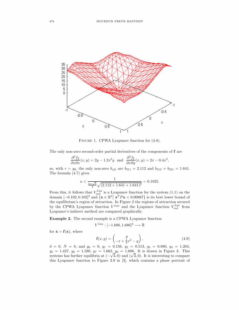
d = 0, N = 8, and y0 = 0, y1 = 0.078, y2 = 0.280, y3 = 0.510, y4 = 0.696,y5 = 0.842, y6 = 0.961, y7 = 1.024, y8 = 1.056. It is drawn in Figure 1.
The indirect method of Lyapunov delivers V Lyaind (x) = xTPx, where
P =(
32 − 1
2− 12 1
).
674 SIGURDUR FREYR HAFSTEIN
Figure 1. CPWA Lyapunov function for (4.8).
The only non-zero second-order partial derivatives of the components of f are
∂2f2∂x∂x
(x, y) = 2y − 1.2x2y and∂2f2∂x∂y
(x, y) = 2x− 0.4x3,
so, with r = y8, the only non-zero bijk are b211 = 2.112 and b212 = b221 = 1.641.The formula (4.7) gives
a <1
5+√
54
√(2.112 + 1.641 + 1.641)2
= 0.1025.
From this, it follows that V Lyaind is a Lyapunov function for the system (1.1) on the
domain [−0.102, 0.102]2 and {x ∈ R2∣∣ xTPx < 0.00867} is its best lower bound of
the equilibrium’s region of attraction. In Figure 2 the regions of attraction securedby the CPWA Lyapunov function V Lya and the Lyapunov function V Lya
ind fromLyapunov’s indirect method are compared graphically.
Example 2. The second example is a CPWA Lyapunov function
V Lya : [−1.686, 1.686]2 −→ R
for x = f(x), where
f(x, y) =(
y−x+ 1
3x3 − y
), (4.9)
d = 0, N = 8, and y0 = 0, y1 = 0.156, y2 = 0.513, y3 = 0.880, y4 = 1.204,y5 = 1.427, y6 = 1.580, y7 = 1.662, y8 = 1.686. It is drawn in Figure 3. Thissystems has further equilibria at (−√
3, 0) and (√
3, 0). It is interesting to comparethis Lyapunov function to Figure 3.9 in [3], which contains a phase portrait of
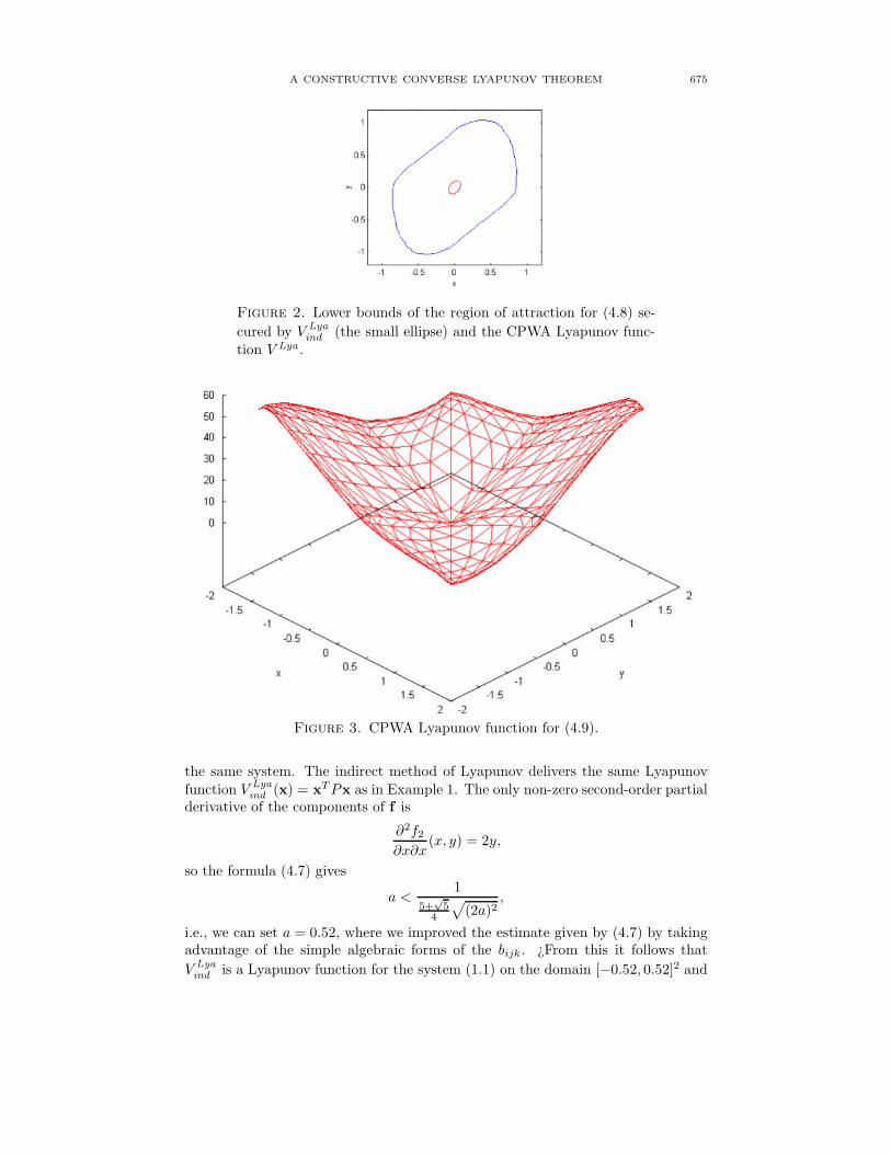
A CONSTRUCTIVE CONVERSE LYAPUNOV THEOREM 675
Figure 2. Lower bounds of the region of attraction for (4.8) se-cured by V Lya
ind (the small ellipse) and the CPWA Lyapunov func-tion V Lya .
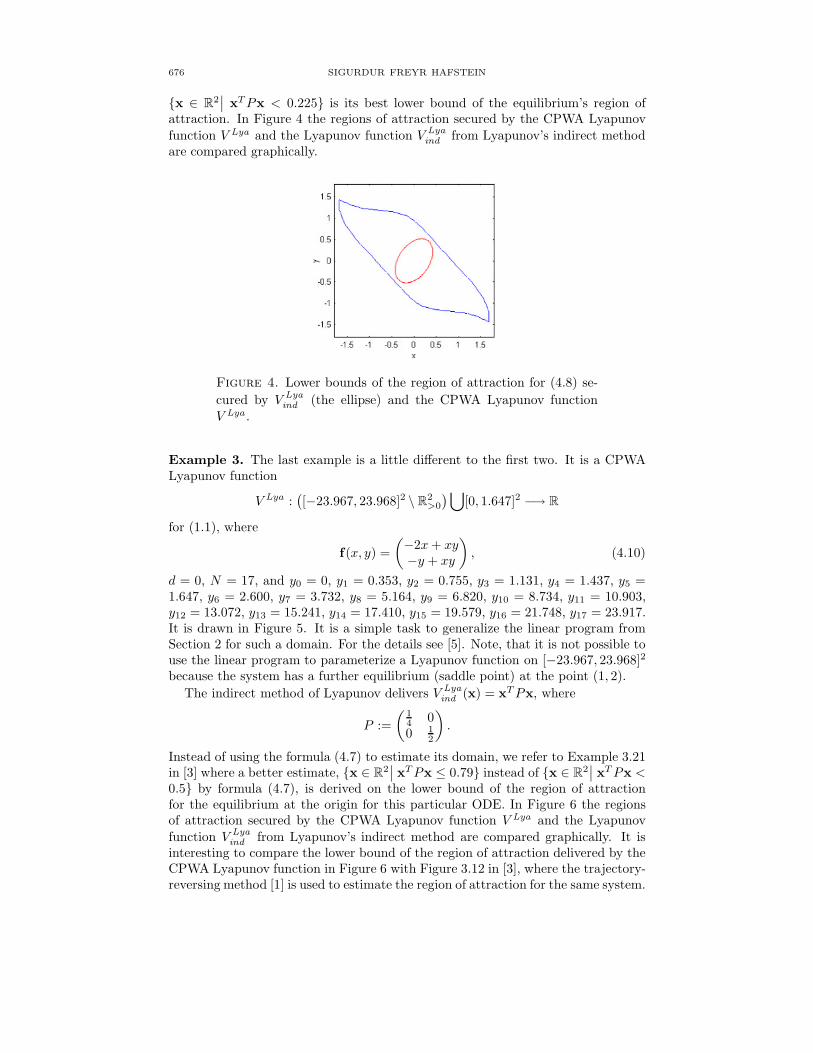
Figure 3. CPWA Lyapunov function for (4.9).
the same system. The indirect method of Lyapunov delivers the same Lyapunovfunction V Lya
ind (x) = xTPx as in Example 1. The only non-zero second-order partialderivative of the components of f is
∂2f2∂x∂x
(x, y) = 2y,
so the formula (4.7) gives
a <1
5+√
54
√(2a)2
,
i.e., we can set a = 0.52, where we improved the estimate given by (4.7) by takingadvantage of the simple algebraic forms of the bijk. ¿From this it follows thatV Lyaind is a Lyapunov function for the system (1.1) on the domain [−0.52, 0.52]2 and
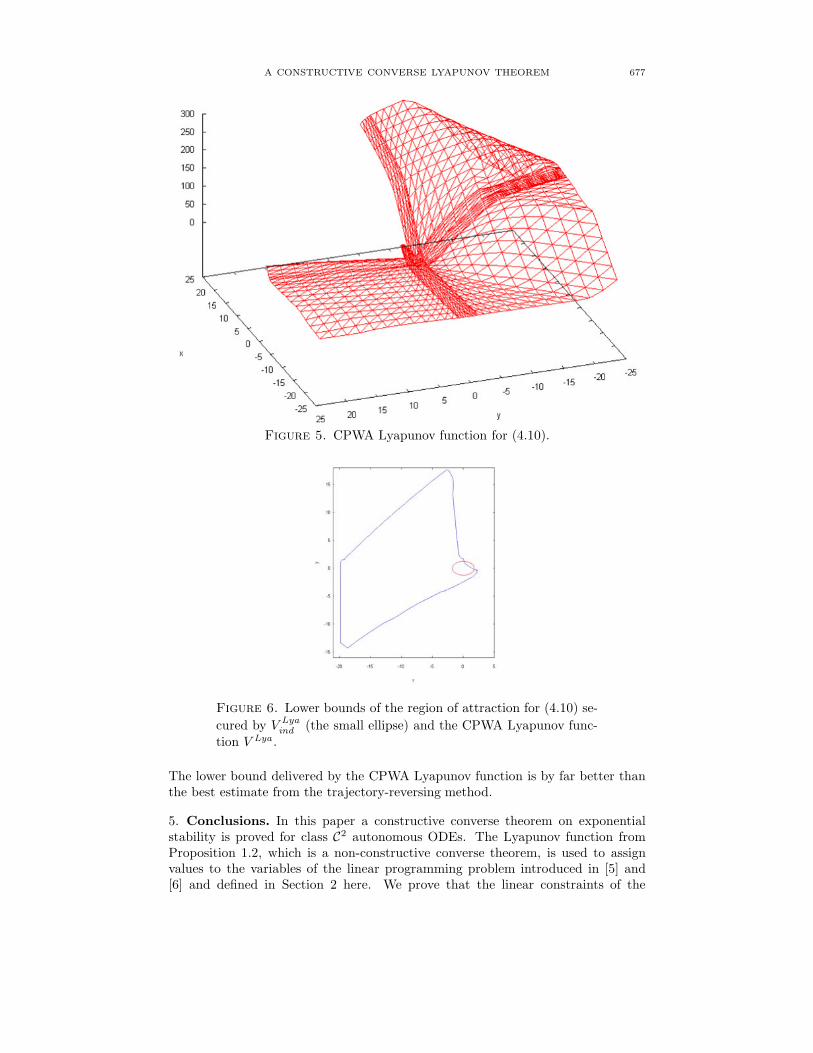
676 SIGURDUR FREYR HAFSTEIN
{x ∈ R2∣∣ xTPx < 0.225} is its best lower bound of the equilibrium’s region of
attraction. In Figure 4 the regions of attraction secured by the CPWA Lyapunovfunction V Lya and the Lyapunov function V Lya
ind from Lyapunov’s indirect methodare compared graphically.
Figure 4. Lower bounds of the region of attraction for (4.8) se-cured by V Lya
ind (the ellipse) and the CPWA Lyapunov functionV Lya .
Example 3. The last example is a little different to the first two. It is a CPWALyapunov function
V Lya :([−23.967, 23.968]2 \ R
2>0
)⋃[0, 1.647]2 −→ R
for (1.1), where
f(x, y) =(−2x+ xy
−y + xy
), (4.10)
d = 0, N = 17, and y0 = 0, y1 = 0.353, y2 = 0.755, y3 = 1.131, y4 = 1.437, y5 =1.647, y6 = 2.600, y7 = 3.732, y8 = 5.164, y9 = 6.820, y10 = 8.734, y11 = 10.903,y12 = 13.072, y13 = 15.241, y14 = 17.410, y15 = 19.579, y16 = 21.748, y17 = 23.917.It is drawn in Figure 5. It is a simple task to generalize the linear program fromSection 2 for such a domain. For the details see [5]. Note, that it is not possible touse the linear program to parameterize a Lyapunov function on [−23.967, 23.968]2
because the system has a further equilibrium (saddle point) at the point (1, 2).The indirect method of Lyapunov delivers V Lya
ind (x) = xTPx, where
P :=(
14 00 1
2
).
Instead of using the formula (4.7) to estimate its domain, we refer to Example 3.21in [3] where a better estimate, {x ∈ R
2∣∣ xTPx ≤ 0.79} instead of {x ∈ R
2∣∣ xTPx <
0.5} by formula (4.7), is derived on the lower bound of the region of attractionfor the equilibrium at the origin for this particular ODE. In Figure 6 the regionsof attraction secured by the CPWA Lyapunov function V Lya and the Lyapunovfunction V Lya
ind from Lyapunov’s indirect method are compared graphically. It isinteresting to compare the lower bound of the region of attraction delivered by theCPWA Lyapunov function in Figure 6 with Figure 3.12 in [3], where the trajectory-reversing method [1] is used to estimate the region of attraction for the same system.
A CONSTRUCTIVE CONVERSE LYAPUNOV THEOREM 677
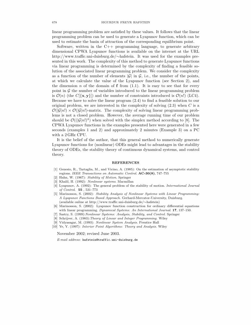
Figure 5. CPWA Lyapunov function for (4.10).
Figure 6. Lower bounds of the region of attraction for (4.10) se-cured by V Lya
ind (the small ellipse) and the CPWA Lyapunov func-tion V Lya .
The lower bound delivered by the CPWA Lyapunov function is by far better thanthe best estimate from the trajectory-reversing method.
5. Conclusions. In this paper a constructive converse theorem on exponentialstability is proved for class C2 autonomous ODEs. The Lyapunov function fromProposition 1.2, which is a non-constructive converse theorem, is used to assignvalues to the variables of the linear programming problem introduced in [5] and[6] and defined in Section 2 here. We prove that the linear constraints of the
678 SIGURDUR FREYR HAFSTEIN
linear programming problem are satisfied by these values. It follows that the linearprogramming problem can be used to generate a Lyapunov function, which can beused to estimate the basin of attraction of the corresponding equilibrium point.
Software, written in the C++ programming language, to generate arbitrarydimensional CPWA Lyapunov functions is available on the internet at the URLhttp://www.traffic.uni-duisburg.de/∼hafstein. It was used for the examples pre-sented in this work. The complexity of this method to generate Lyapunov functionsvia linear programming is determined by the complexity of finding a feasible so-lution of the associated linear programming problem. We consider the complexityas a function of the number of elements |G| in G, i.e., the number of the points,at which we calculate the value of the Lyapunov function (see Section 2), andthe dimension n of the domain of f from (1.1). It is easy to see that for everypoint in G the number of variables introduced to the linear programming problemis O(n) (the C[{x,y}]) and the number of constraints introduced is O(n!) (LC4).Because we have to solve the linear program (2.4) to find a feasible solution to ouroriginal problem, we are interested in the complexity of solving (2.3) when C is aO(|G|n!) × O(|G|n!)-matrix. The complexity of solving linear programming prob-lems is not a closed problem. However, the average running time of our problemshould be O((|G|n!)4) when solved with the simplex method according to [8]. TheCPWA Lyapunov functions in the examples presented here were generated in a fewseconds (examples 1 and 2) and approximately 2 minutes (Example 3) on a PCwith a 2GHz CPU.
It is the belief of the author, that this general method to numerically generateLyapunov functions for (nonlinear) ODEs might lead to advantages in the stabilitytheory of ODEs, the stability theory of continuous dynamical systems, and controltheory.
REFERENCES
[1] Genesio, R., Tartaglia, M., and Vicino, A. (1985): On the estimation of asymptotic stabilityregions. IEEE Transactions on Automatic Control. AC-30(8), 747–755
[2] Hahn, W. (1967): Stability of Motion. Springer[3] Khalil, H. (1992): Nonlinear systems. Macmillan[4] Lyapunov, A. (1992): The general problem of the stability of motion. International Journal
of Control. 55 , 531–773[5] Marinosson, S. (2002): Stability Analysis of Nonlinear Systems with Linear Programming:
A Lyapunov Functions Based Approach. Gerhard-Mercator-University, Duisburg.(available online at http://www.traffic.uni-duisburg.de/∼hafstein)
[6] Marinosson, S. (2002): Lyapunov function construction for ordinary differential equationswith linear programming. Dynamical Systems: An International Journal. 17, 137–150.
[7] Sastry, S. (1999):Nonlinear Systems: Analysis, Stability, and Control. Springer[8] Schrijver, A. (1983):Theory of Linear and Integer Programming. Wiley[9] Vidyasagar, M. (1993): Nonlinear System Analysis. Prentice Hall
[10] Ye, Y. (1997): Interior Point Algorithms: Theory and Analysis. Wiley
November 2002; revised June 2003.E-mail address: [email protected]
Related Documents