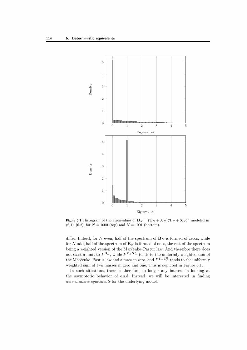
6 Deterministic equivalents 6.1 Introduction to deterministic equivalents The first applications of random matrix theory to the field of wireless communications, e.g., [Tse and Hanly, 1999; Tse and Verd´ u, 2000; Verd´ u and Shamai, 1999], originally dealt with the limiting behavior of some simple random matrix models. In particular, these results are attractive as these limiting behaviors only depend on the limiting eigenvalue distribution of the deterministic matrices of the model. This is in fact the case of all the results we have derived and introduced so far; for instance, Theorem 3.13 unveils the limiting behavior of the e.s.d. of B N = A N + X H N T N X N when both e.s.d. of A N and T N converge toward given deterministic distribution functions and X N is random with i.i.d. entries. However, for practical applications, it might turn out that: (i) the e.s.d. of A N or T N do not necessarily converge to a limiting distribution; (ii) even if the e.s.d. of the deterministic matrices in the model do all converge to their respective l.s.d., the e.s.d. of the output matrix B N might not converge. This is of course not the case in Theorem 3.13, but we will show that this may happen for more involved models, e.g. the models treated by [Couillet et al., 2011a] and [Hachem et al., 2007]. Let us introduce a simple scenario for which the e.s.d. of the random matrix does not converge. This example is borrowed from [Hachem et al., 2007]. Define X N ∈ C 2N×2N as X N = X 0 N 0 0 0 (6.1) with the entries of X 0 N being i.i.d. with zero mean and variance 1 N . Consider in addition the matrix T N ∈ C 2N×2N defined as T N = I N 0 00 ,N even 00 0 I N ,N odd. (6.2) Then, taking B N =(T N + X N )(T N + X N ) H , F B 2N and F B 2N+1 both converge weakly towards limit distributions, as N →∞, but those distributions

Welcome message from author
This document is posted to help you gain knowledge. Please leave a comment to let me know what you think about it! Share it to your friends and learn new things together.
Transcript

6 Deterministic equivalents
6.1 Introduction to deterministic equivalents
The first applications of random matrix theory to the field of wireless
communications, e.g., [Tse and Hanly, 1999; Tse and Verdu, 2000; Verdu and
Shamai, 1999], originally dealt with the limiting behavior of some simple random
matrix models. In particular, these results are attractive as these limiting
behaviors only depend on the limiting eigenvalue distribution of the deterministic
matrices of the model. This is in fact the case of all the results we have derived
and introduced so far; for instance, Theorem 3.13 unveils the limiting behavior of
the e.s.d. of BN = AN + XHNTNXN when both e.s.d. of AN and TN converge
toward given deterministic distribution functions and XN is random with i.i.d.
entries. However, for practical applications, it might turn out that:
(i) the e.s.d. of AN or TN do not necessarily converge to a limiting distribution;
(ii) even if the e.s.d. of the deterministic matrices in the model do all converge to
their respective l.s.d., the e.s.d. of the output matrix BN might not converge.
This is of course not the case in Theorem 3.13, but we will show that this may
happen for more involved models, e.g. the models treated by [Couillet et al.,
2011a] and [Hachem et al., 2007].
Let us introduce a simple scenario for which the e.s.d. of the random matrix
does not converge. This example is borrowed from [Hachem et al., 2007]. Define
XN ∈ C2N×2N as
XN =
(X′N 0
0 0
)(6.1)
with the entries of X′N being i.i.d. with zero mean and variance 1N . Consider in
addition the matrix TN ∈ C2N×2N defined as
TN =
(
IN 0
0 0
), N even(
0 0
0 IN
), N odd.
(6.2)
Then, taking BN = (TN + XN )(TN + XN )H, FB2N and FB2N+1 both
converge weakly towards limit distributions, as N →∞, but those distributions
114 6. Deterministic equivalents
0 1 2 3 4 50
1
2
3
4
5
Eigenvalues
Den
sity
0 1 2 3 4 50
1
2
3
4
5
Eigenvalues
Den
sity
Figure 6.1 Histogram of the eigenvalues of BN = (TN + XN )(TN + XN )H modeled in(6.1)–(6.2), for N = 1000 (top) and N = 1001 (bottom).
differ. Indeed, for N even, half of the spectrum of BN is formed of zeros, while
for N odd, half of the spectrum of BN is formed of ones, the rest of the spectrum
being a weighted version of the Marcenko–Pastur law. And therefore there does
not exist a limit to FBN , while FXNXHN tends to the uniformly weighted sum of
the Marcenko–Pastur law and a mass in zero, and FTNTHN tends to the uniformly
weighted sum of two masses in zero and one. This is depicted in Figure 6.1.
In such situations, there is therefore no longer any interest in looking at
the asymptotic behavior of e.s.d. Instead, we will be interested in finding
deterministic equivalents for the underlying model.

6.2. Techniques for deterministic equivalents 115
Definition 6.1. Consider a series of Hermitian random matrices B1,B2, . . .,
with BN ∈ CN×N and a series f1, f2, . . . of functionals of 1× 1, 2× 2, . . .
matrices. A deterministic equivalent of BN for the functional fN is a series
B◦1,B◦2, . . . where B◦N ∈ CN×N , of deterministic matrices, such that
limN→∞
fN (BN )− fN (B◦N )→ 0
where the convergence will often be with probability one. Note that fN (B◦N )
does not need to have a limit as N →∞. We will similarly call gN , fN (B◦N )
the deterministic equivalent of fN (BN ), i.e. the deterministic series g1, g2, . . .
such that fN (BN )− gN → 0 in some sense.
We will often take fN to be the normalized trace of (BN − zIN )−1, i.e. the
Stieltjes transform of FBN . When fN (B◦N ) does not have a limit, the Marcenko–
Pastur method, developed in Section 3.2, will fail. This is because, at some point,
all the entries of the underlying matrices will have to be taken into account and
not only the diagonal entries, as in the proof we provided in Section 3.2. However,
the Marcenko–Pastur method can be tweaked adequately into a technique that
can cope with deterministic equivalents. In the following, we first introduce this
technique, which we will call the Bai and Silverstein technique, and then discuss
an alternative technique, known as the Gaussian method, which is particularly
suited to random matrix models with Gaussian entries. Hereafter, we detail these
methods by successively proving two (similar) results of importance in wireless
communications, see further Chapters 13–14.
6.2 Techniques for deterministic equivalents
6.2.1 Bai and Silverstein method
We first introduce a deterministic equivalent for the model
BN =
K∑k=1
R12
kXkTkXHkR
12
k + A
where the K matrices Xk have i.i.d. entries for each k, mutually independent
for different k, and the matrices T1, . . . ,TK , R1, . . . ,RK and A are ‘bounded’
in some sense to be defined later. This is more general than the model of
Theorem 3.13 in several respects:
(i) left product matrices Rk, 1 ≤ k ≤ K, have been introduced. As an exercise,
it can already be verified that a l.s.d. for the model R121 X1T1X
H1 R
121 + A may
not exist even if FR1 and FA both converge vaguely to deterministic limits,
unless some severe additional constraint is put on the eigenvectors of R1 and
A, e.g. R1 and A are codiagonalizable. This suggests that the Marcenko–
Pastur method will fail to treat this model;

116 6. Deterministic equivalents
(ii) a sum of K such models is considered (K does not grow along with N here);
(iii) the e.s.d. of the (possibly random) matrices Tk and Rk are not required to
converge.
While the result to be introduced hereafter is very likely to hold for X1, . . . ,XK
with non-identically distributed entries (as long as they have common mean and
variance and some higher order moment condition), we only present here the
result where these entries are identically distributed, which is less general than
the conditions of Theorem 3.13.
Theorem 6.1 ([Couillet et al., 2011a]). Let K be some positive integer. For
some integer N , let
BN =
K∑k=1
R12
kXkTkXHkR
12
k + A
be an N ×N matrix with the following hypotheses, for all k ∈ {1, . . . ,K}
1. Xk =(
1√nkXk,ij
)∈ CN×nk is such that the Xk,ij are identically distributed
for all N , i, j, independent for each fixed N , and E|Xk,11 − EXk,11|2 = 1;
2. R12
k ∈ CN×N is a Hermitian non-negative definite square root of the non-
negative definite Hermitian matrix Rk;
3. Tk = diag(τk,1, . . . , τk,nk) ∈ Cnk×nk , nk ∈ N∗, is diagonal with τk,i ≥ 0;
4. the sequences FT1 , FT2 , . . . and FR1 , FR2 , . . . are tight, i.e. for all ε > 0, there
exists M > 0 such that 1− FTk(M) < ε and 1− FRk(M) < ε for all nk, N ;
5. A ∈ CN×N is Hermitian non-negative definite;
6. denoting ck = N/nk, for all k, there exist 0 < a < b <∞ for which
a ≤ lim infNck ≤ lim sup
Nck ≤ b. (6.3)
Then, as all N and nk grow large, with ratio ck, for z ∈ C \ R+, the Stieltjes
transform mBN (z) of BN satisfies
mBN (z)−mN (z)a.s.−→ 0 (6.4)
where
mN (z) =1
Ntr
(A +
K∑k=1
∫τkdF
Tk(τk)
1 + ckτkeN,k(z)Rk − zIN
)−1
(6.5)
and the set of functions eN,1(z), . . . , eN,K(z) forms the unique solution to the K
equations
eN,i(z) =1
Ntr Ri
(A +
K∑k=1
∫τkdF
Tk(τk)
1 + ckτkeN,k(z)Rk − zIN
)−1
(6.6)
such that sgn(=[eN,i(z)]) = sgn(=[z]), if z ∈ C \ R, and eN,i(z) > 0 if z is real
negative.

6.2. Techniques for deterministic equivalents 117
Moreover, for any ε > 0, the convergence of Equation (6.4) is uniform over
any region of C bounded by a contour interior to
C \ ({z : |z| ≤ ε} ∪ {z = x+ iv : x > 0, |v| ≤ ε}) .
For all N , the function mN is the Stieltjes transform of a distribution function
FN , and
FBN − FN ⇒ 0
almost surely as N →∞.
In [Couillet et al., 2011a], Theorem 6.1 is completed by the following result.
Theorem 6.2. Under the conditions of Theorem 6.1, the scalars
eN,1(z), . . . , eN,K(z) are also explicitly given by:
eN,i(z) = limt→∞
etN,i(z)
where, for all i, e0N,i(z) = −1/z and, for t ≥ 1
etN,i(z) =1
Ntr Ri
A +
K∑j=1
∫τjdF
Tj (τj)
1 + cjτjet−1N,j(z)
Rj − zIN
−1
.
This result, which ensures the convergence of the classical fixed-point
algorithm for an adequate initial condition, is of fundamental importance for
practical purposes as it ensures that the eN,1(z), . . . , eN,K(z) can be determined
numerically in a deterministic way. Since the proof of Theorem 6.2 relies heavily
on the proof of Theorem 6.1, we will prove Theorem 6.2 later.
Several remarks are in order before we prove Theorem 6.1. We have given
much detail on the conditions for Theorem 6.1 to hold. We hereafter discuss the
implications of these conditions. Condition 1 requires that theXk,ij be identically
distributed across N, i, j, but not necessarily across k. Note that the identical
distribution condition could be further released under additional mild conditions
(such as all entries must have a moment of order 2 + ε, for some ε > 0), see
Theorem 3.13. Condition 4 introduces tightness requirements on the e.s.d. of Rk
and Tk. Tightness can be seen as the probabilistic equivalent to boundedness
for deterministic variables. Tightness ensures here that no mass of the FRk and
FTk escapes to infinity as n grows large. Condition 6 is more general than the
requirement that ck has a limit as it allows ck, for all k, to wander between two
positive values.
From a practical point of view, R12
KXkT12
k will often be used to model a
multiple antenna N × nk channel with i.i.d. entries with transmit and receive
correlations. From the assumptions of Theorem 6.1, the correlation matrices Rk
and Tk are only required to be ‘bounded’ in the sense of tightness of their e.s.d.
This means that, as the number of antennas grows, the eigenvalues of Rk and Tk

118 6. Deterministic equivalents
can only blow up with increasingly low probability. If we increase the number N
of antennas on a bounded three-dimensional space, then the rough tendency is
for the eigenvalues of Tk and Rk to be all small except for a few of them, which
grow large but have a probability of order O(1/N), see, e.g., [Pollock et al., 2003].
In that context, Theorem 6.1 holds, i.e. for N →∞, FBN − FN ⇒ 0.
It is also important to remark that the matrices Tk are constrained to be
diagonal. This is unimportant when the matrices Xk are assumed Gaussian in
practical applications, as the Xk, being bi-unitarily invariant, can be multiplied
on the right by any deterministic unitary matrix without altering the final
result. This limitation is linked to the technique used for proving Theorem 6.1.
For mathematical completion, though, it would be convenient for the matrices
Tk to be unconstrained. We mention that Zhang and Bai [Zhang, 2006]
derive the limiting spectral distribution of the model BN = R121 X1T1X
H1 R
121 for
unconstrained Hermitian T1, using a different approach than that presented
below.
For practical applications, it will be easier in the following to write (6.6) in a
more symmetric way. This is discussed in the following remark.
Remark 6.1. In the particular case where A = 0, the K implicit Equations (6.6)
can be developed into the 2K linked equations
eN,i(z) =1
Ntr Ri
(−z
[IN +
K∑k=1
ek(z)Rk
])−1
eN,i(z) =1
nitr Ti (−z [Ini + cieN,i(z)Ti])
−1 (6.7)
whose symmetric aspect is both more readable and more useful for practical
reasons that will be evidenced later in Chapters 13–14. As a consequence, mN (z)
in (6.5) becomes
mN (z) =1
Ntr
(−z
[IN +
K∑k=1
eN,k(z)Rk
])−1
.
In the literature and, as a matter of fact, in some deterministic equivalents
presented later in this chapter, the variables eN,i(z) may be normalized by 1ni
instead of 1N in order to avoid carrying the factor ci in front of eN,i(z) in the
second fixed-point equation of (6.7). In the application chapters, Chapters 12–15,
depending on the situation, either one or the other convention will be taken.
We present hereafter the general techniques, based on the Stieltjes transform,
to prove Theorem 6.1 and other similar results introduced in this section.
As opposed to the proof of the Marcenko–Pastur law, we cannot prove that
that there exists a space of probability one over which mBN (z)→ m(z) for
all z ∈ C \ R+, for a certain limiting function m. Instead, we prove that there
exists a space of probability one over which mBN (z)−mN (z)→ 0 for all z, for
a certain series of Stieltjes transforms m1(z),m2(z), . . .. There are in general
6.2. Techniques for deterministic equivalents 119
two main approaches to prove this convergence. The first option is a point-
wise approach that consists in proving the convergence for all z in a compact
subspace of C \ R+ having a limit point. Invoking Vitali’s convergence theorem,
similar to the proof of the Marcenko–Pastur law, we then prove the convergence
for all z ∈ C \ R+. In the coming proof, we will take z ∈ C+. In the proof of
Theorem 6.17, we will take z real negative. The second option is a functional
approach in which the objects under study are not mBN (z) and mN (z) taken
at a precise point z ∈ C \ R+ but rather mBN (z) and mN (z) seen as functions
lying in the space of Stieltjes transforms of distribution functions with support
on R+. The convergence mBN (z)−mN (z)a.s.−→ 0 is in this case functional and
Vitali’s convergence theorem is not called for. This is the approach followed in,
e.g., [Hachem et al., 2007]. The latter is not detailed in this book.
The first step of the general proof, for either option, consists in determining
mN (z). For this, similar to the Marcenko–Pastur proof, we develop the expression
of mBN (z), seeking for a limiting result of the kind
mBN (z)− hN (mBN (z); z)a.s.−→ 0
for some deterministic function hN , possibly depending on N . Such an expression
allows us to infer the nature of a deterministic approximation mN (z) of mBN (z)
as a particular solution of the equation in m
m− hN (m; z) = 0. (6.8)
This equation rarely has a unique point-wise solution, i.e. for every z, but often
has a unique functional solution z → mN (z) that is the Stieltjes transform of a
distribution function. If the point-wise approach is followed, a unique point-wise
solution of (6.8) can often be narrowed down to a certain subspace of C for z lying
in some other subspace of C. In Theorem 6.1, there exists a single solution in C+
when z ∈ C+, a single solution in C− when z ∈ C−, and a single positive solution
when z is real negative. Standard holomorphicity arguments on the function
mN (z) then ensure that z → mN (z) is the unique Stieltjes transform satisfying
hN (mN (z); z) = mN (z). When using the functional approach, this fact tends to
be proved more directly. In the coming proof of Theorem 6.1, we will prove point-
wise uniqueness by assuming, as per standard techniques, the alleged existence
of two distinct solutions and prove a contradiction. An alternative approach is
to prove that the fixed-point algorithm
m0 ∈ D
mt+1 = hN (mt; z), t ≥ 0
always converges to mN (z), where D is taken to be either R−, C+ or C−. This
approach, when valid (in some involved cases, convergence may not always arise),
is doubly interesting as it allows both (i) to prove point-wise uniqueness for z
taken in some subset of C \ R+, leading to uniqueness of the Stieltjes transform
using again holomorphicity arguments, and (ii) to provide an explicit algorithm
120 6. Deterministic equivalents
to compute mN (z) for z ∈ D, which is in particular of interest for practical
applications when z = −σ2 < 0. In the proof of Theorem 6.1, we will introduce
both results for completion. In the proof of Theorem 6.17, we will directly proceed
to proving the convergence of the fixed-point algorithm for z real negative.
When the uniqueness of the Stieltjes transform mN (z) has been made clear,
the last step is to prove that, in the large N limit
mBN (z)−mN (z)a.s.−→ 0.
This step is not so immediate. To this point, we indeed only know that
mBN (z)− hN (mBN (z); z)a.s.−→ 0 and mN (z)− hN (mN (z); z) = 0. This does not
imply immediately that mBN (z)−mN (z)a.s.−→ 0. If there are several point-wise
solutions to m− hN (m; z) = 0, we need to verify that mN (z) was chosen to be
the one that will eventually satisfy mBN (z)−mN (z)a.s.−→ 0. This will conclude
the proof.
We now provide the specific proof of Theorem 6.1. In order to determine the
above function hN , we first develop the Marcenko–Pastur method (for simplicity
for K = 2 and A = 0). We will realize that this method fails unless all Rk and
A are constrained to be co-diagonalizable. To cope with this limitation, we will
introduce the more powerful Bai and Silverstein method, whose idea is to guess
along the derivations the suitable form of hN . In fact, as we will shortly realize,
the problem is slightly more difficult here as we will not be able to find such
a function hN (which may actually not exist at all in the first place). We will
however be able to find functions fN,i such that, for each i
eBN ,i(z)− fN,i(eBN ,1(z), . . . , eBN ,K(z); z)a.s.−→ 0
where eBN ,i(z) ,1N tr Ri(BN − zIN )−1. We will then look for a function eN,i(z)
that satisfies
eN,i(z) = fN,i(eN,1(z), . . . , eN,K(z); z).
From there, it will be easy to determine a further function gN such that
mBN (z)− gN (eBN ,1(z), . . . , eBN ,K(z); z)a.s.−→ 0
and
mN (z)− gN (eN,1(z), . . . , eN,K(z); z) = 0.
We will therefore have finally
mBN (z)−mN (z)a.s.−→ 0.
Proof of Theorem 6.1. In order to have a first insight on what the deterministic
equivalent mN of mBN may look like, the Marcenko–Pastur method will be
applied with the (strong) additional assumption that A and all Rk, 1 ≤ k ≤ K,
are diagonal and that the e.s.d. FTk , FRk converge for all k as N grows large.
In this scenario, mBN has a limit when N →∞ and the method, however more
tedious than in the proof of the Marcenko–Pastur law, leads naturally to mN .

6.2. Techniques for deterministic equivalents 121
Consider the case when K = 2, A = 0 for simplicity and denote Hk =
R12
kXkT12
k . Following similar steps as in the proof of the Marcenko–Pastur law,
we start with matrix inversion lemmas(H1H
H1 + H2H
H2 − zIN
)−1
11
=
[−z − z[hH
1 hH2 ]
([UH
1
UH2
][U1U2]− zIn1+n2
)−1 [h1
h2
]]−1
with the definition HHi = [hiU
Hi ]. Using the block matrix inversion lemma, the
inner inversed matrix in this expression can be decomposed into four submatrices.
The upper-left n1 × n1 submatrix reads:(−zUH
1 (U2UH2 − zIN−1)−1U1 − zIn1
)−1
while, for the second block diagonal entry, it suffices to revert all ones in twos and
vice-versa. Taking the limits, using Theorem 3.4 and Theorem 3.9, we observe
that the two off-diagonal submatrices will not play a role, and we finally have(H1H
H1 + H2H
H2 − zIN
)−1
11
'[−z − zr11
1
n1tr T1
(−zHH
1 (H2HH2 − zIN )−1H1 − zIn1
)−1
−zr211
n2tr T2
(−zHH
2 (H1HH1 − zIN )−1H1 − zIn2
)−1]−1
where the symbol “'” denotes some kind of yet unknown large N
convergence and where we denoted rij the jth diagonal entry of Ri.
Observe that we can proceed to a similar derivation for the matrix
T1
(−zHH
1 (H2HH2 − zIN )−1H1 − zIn1
)−1that now appears. Denoting now Hi =
[hiUi], we have indeed[T1
(−zHH
1 (H2HH2 − zIN )−1H1 − zIn1
)−1]
11
= τ11
[−z − zhH
1
(U1U
H1 + H2H
H2 − zIN
)−1
h1
]−1
' τ11
[−z − zc1τ11
1
Ntr R1
(H1H
H1 + H2H
H2 − zIN
)−1]−1
with τij the jth diagonal entry of Ti. The limiting result here arises from the trace
lemma, Theorem 3.4 along with the rank-1 perturbation lemma, Theorem 3.9.
The same result holds when changing ones in twos.
We now denote by ei and ei the (almost sure) limits of the random quantities
eBN ,i =1
Ntr Ri
(H1H
H1 + H2H
H2 − zIN
)−1
and
eBN ,i =1
Ntr Ti
(−zHH
1 (H2HH2 − zIN )−1H1 − zIn1
)−1

122 6. Deterministic equivalents
respectively, as FTi and FRi converge in the large N limit. These limits exist
here since we forced R1 and R2 to be co-diagonalizable. We find
ei = limN→∞
1
Ntr Ri (−zeBN ,iR1 − zeBN ,iR2 − zIN )−1
ei = limN→∞
1
Ntr Ti (−zcieBN ,iTi − zIni)
−1
where the type of convergence is left to be determined. From this short calculus,
we can infer the form of (6.7).
This derivation obviously only provides a hint on the deterministic equivalent
for mN (z). It also provides the aforementioned observation that mN (z) is not
itself solution of a fixed-point equation, although eN,1(z), . . . , eN,K(z) are. To
prove Theorem 6.1, irrespective of the conditions imposed on R1, . . . ,RK ,
T1, . . . ,TK and A, we will successively go through four steps, given below.
For readability, we consider the case K = 1 and discard the useless indexes.
The generalization to K ≥ 1 is rather simple for most of the steps but requires
cumbersome additional calculus for some particular aspects. These pieces of
calculus are not interesting here, the reader being invited to refer to [Couillet
et al., 2011a] for more details. The four-step procedure is detailed below.
• Step 1. We first seek a function fN , such that, for z ∈ C+
eBN (z)− fN (eBN (z); z)a.s.−→ 0
as N →∞, where eBN (z) = 1N tr R(BN − zIN )−1. This function fN was
already inferred by the Marcenko–Pastur approach. Now, we will make this
step rigorous by using the Bai and Silverstein approach, as is done in,
e.g., [Dozier and Silverstein, 2007a; Silverstein and Bai, 1995]. Basically, the
function fN will be found using an inference procedure. That is, starting
from a very general form of fN , i.e. fN = 1N tr RD−1 for some matrix D ∈
CN×N (not yet written as a function of z or eBN (z)), we will evaluate the
difference eBN (z)− fN and progressively discover which matrix D will make
this difference increasingly small for large N .
• Step 2. For fixed N , we prove the existence of a solution to the implicit
equation in the dummy variable e
fN (e; z) = e. (6.9)
This is often performed by proving the existence of a sequence eN,1, eN,2, . . .,
lying in a compact space such that fN (eN,k; z)− eN,k converges to zero, in
which case there exists at least one converging subsequence of eN,1, eN,2, . . .,
whose limit eN satisfies (6.9).
• Step 3. Still for fixed N , we prove the uniqueness of the solution of (6.9)
lying in some specific space and we call this solution eN (z). This is classically
performed by assuming the existence of a second distinct solution and by
exhibiting a contradiction.
6.2. Techniques for deterministic equivalents 123
• Step 4. We finally prove that
eBN (z)− eN (z)a.s.−→ 0
and, similarly, that
mBN (z)−mN (z)a.s.−→ 0
as N →∞, with mN (z) , gN (eN (z); z) for some function gN .
At first, following the works of Bai and Silverstein, a truncation, centralization,
and rescaling step is required to replace the matrices X, R, and T by truncated
versions X, R, and T, respectively, such that the entries of X have zero mean,
‖X‖ ≤ k log(N), for some constant k, ‖R‖ ≤ log(N) and ‖T‖ ≤ log(N). Similar
to the truncation steps presented in Section 3.2.2, it is shown in [Couillet et al.,
2011a] that these truncations do not restrict the generality of the final result for
{FT} and {FR} forming tight sequences, that is:
F R12 XTXHR
12 − FR
12 XTXHR
12 ⇒ 0
almost surely, as N grows large. Therefore, we can from now on work with these
truncated matrices. We recall that the main interest of this procedure is to be
able to derive a deterministic equivalent (or l.s.d.) of the underlying random
matrix model without the need for any moment assumption on the entries of X,
by replacing the entries of X by truncated random variables that have moments
of all orders. Here, the interest is in fact two-fold, since, in addition to truncating
the entries of X, also the entries of T and R are truncated in order to be able
to prove results for matrices T and R that in reality have eigenvalues growing
very large but that will be assumed to have entries bounded by log(N). For
readability in the following, we rename X, T, and R the truncated matrices.
Remark 6.2. Alternatively, expected values can be used to discard the stochastic
character. This introduces an additional convergence step, which is the approach
followed by Hachem, Najim, and Loubaton in several publications, e.g., [Hachem
et al., 2007] and [Dupuy and Loubaton, 2009]. This additional step consists in
first proving the almost sure weak convergence of FBN −GN to zero, for GNsome auxiliary deterministic distribution (such as GN = E[FBN ]), before proving
the convergence GN − FN ⇒ 0.
Step 1. First convergence stepWe start with the introduction of two fundamental identities.
Lemma 6.1 (Resolvent identity). For invertible A and B matrices, we have the
identity
A−1 −B−1 = −A−1(A−B)B−1.

124 6. Deterministic equivalents
This can be verified easily by multiplying both sides on the left by A and on
the right by B (the resulting equality being equivalent to Lemma 6.1 for A and
B invertible).
Lemma 6.2 (A matrix inversion lemma, (2.2) in [Silverstein and Bai, 1995]).
Let A ∈ CN×N be Hermitian invertible, then, for any vector x ∈ CN and any
scalar τ ∈ C, such that A + τxxH is invertible
xH(A + τxxH)−1 =xHA−1
1 + τxHA−1x.
This is verified by multiplying both sides by A + τxxH from the right.
Lemma 6.1 is often referred to as the resolvent identity, since it will be
mainly used to take the difference between matrices of type (X− zIN )−1 and
(Y − zIN )−1, which we remind are called the resolvent matrices of X and Y,
respectively.
The fundamental idea of the approach by Bai and Silverstein is to guess the
deterministic equivalent of mBN (z) by writing it under the form 1N tr D−1 at first,
where D needs to be determined. This will be performed by taking the difference
mBN (z)− 1N tr D−1 and, along the lines of calculus, successively determining the
good properties D must satisfy so that the difference tends to zero almost surely.
We then start by taking z ∈ C+ and D ∈ CN×N some invertible matrix whose
normalized trace would ideally be close to mBN (z) = 1N tr(BN − zIN )−1. We
then write
D−1 − (BN − zIN )−1 = D−1(A + R12 XTXHR
12 − zIN −D)(BN − zIN )−1
(6.10)
using Lemma 6.1.
Notice here that, since BN is Hermitian non-negative definite, and z ∈ C+, the
term (BN − zIN )−1 has uniformly bounded spectral norm (bounded by 1/=[z]).
Since D−1 is desired to be close to (BN − zIN )−1, the same property should also
hold for D−1. In order for the normalized trace of (6.10) to be small, we need
therefore to focus exclusively on the inner difference on the right-hand side. It
seems then interesting at this point to write D , A− zIN + pNR for pN left to
be defined. This leads to
D−1 − (BN − zIN )−1
= D−1R12
(XTXH
)R
12 (BN − zIN )−1 − pND−1R(BN − zIN )−1
= D−1n∑j=1
τjR12 xjx
Hj R
12 (BN − zIN )−1 − pND−1R(BN − zIN )−1
where in the second equality we used the fact that XTXH =∑nj=1 τjxjx
Hj ,
with xj ∈ CN the jth column of X and τj the jth diagonal element of T.
Denoting B(j) = BN − τjR12 xjx
Hj R
12 , i.e. BN with column j removed, and using
6.2. Techniques for deterministic equivalents 125
Lemma 6.2 for the matrix B(j), we have:
D−1 − (BN − zIN )−1
=
n∑j=1
τjD−1R
12 xjx
Hj R
12 (B(j) − zIN )−1
1 + τjxHR12 (B(j) − zIN )−1R
12 xj− pND−1R(BN − zIN )−1.
Taking the trace on each side, and recalling that, for a vector x and a matrix
A, tr(AxxH) = tr(xHAx) = xHAx, this becomes
1
Ntr D−1 − 1
Ntr(BN − zIN )−1
=1
N
n∑j=1
τjxHj R
12 (B(j) − zIN )−1D−1R
12 xj
1 + τjxHR12 (B(j) − zIN )−1R
12 xj− pN
1
Ntr R(BN − zIN )−1D−1
(6.11)
where quadratic forms of the type xHAx appear.
Remembering the trace lemma, Theorem 3.4, which can a priori be applied to
the terms xHj R
12 (B(j) − zIN )−1D−1R
12 xj since xj is independent of the matrix
R12 (B(j) − zIN )−1D−1R
12 , we notice that by setting
pN =1
n
n∑j=1
τj
1 + τjc1N tr R(BN − zIN )−1
.
Equation (6.11) becomes
1
Ntr D−1 − 1
Ntr(BN − zIN )−1
=1
N
n∑j=1
τj
[xHj R
12 (B(j) − zIN )−1D−1R
12 xj
1 + τjxHR12 (B(j) − zIN )−1R
12 xj−
1n tr R(BN − zIN )−1D−1
1 + cτj1N tr R(BN − zIN )−1
](6.12)
which is suspected to converge to zero as N grows large, since both the
numerators and the denominators converge to one another. Let us assume
for the time being that the difference effectively goes to zero almost surely.
Equation (6.12) implies
1
Ntr(BN − zIN )−1 − 1
Ntr
A +1
n
n∑j=1
τjR
1 + τjc1N tr R(BN − zIN )−1
− zIN
−1
a.s.−→ 0
which determines mBN (z) = 1N tr(BN − zIN )−1 as a function of the trace
1N tr R(BN − zIN )−1, and not as a function of itself. This is the observation
made earlier when we obtained a first hint on the form of mN (z) using the
Marcenko–Pastur method, according to which we cannot find a function fNsuch that mBN (z)− fN (mBN (z), z)
a.s.−→ 0. Instead, running the same steps as

126 6. Deterministic equivalents
above, it is rather easy now to observe that
1
Ntr RD−1 − 1
Ntr R(BN − zIN )−1
=1
N
n∑j=1
τj
[xHj R
12 (B(j) − zIN )−1RD−1R
12 xj
1 + τjxHj R
12 (B(j) − zIN )−1R
12 xj−
1n tr R(BN − zIN )−1RD−1
1 + τjcN tr R(BN − zIN )−1
]
where ‖R‖ ≤ logN . Then, denoting eBN (z) , 1N tr R(BN − zIN )−1, we suspect
to have also
eBN (z)− 1
Ntr R
A +1
n
n∑j=1
τj1 + τjceBN (z)
R− zIN
−1
a.s.−→ 0
and
mBN (z)− 1
Ntr
A +1
n
n∑j=1
τj1 + τjceBN (z)
R− zIN
−1
a.s.−→ 0
which is exactly what was required, i.e. eBN (z)− fN (eBN (z); z)a.s.−→ 0 with
fN (e; z) =1
Ntr R
A +1
n
n∑j=1
τj1 + τjce
R− zIN
−1
and mBN (z)− gN (eBN (z); z)a.s.−→ 0 with
gN (e; z) =1
Ntr
A +1
n
n∑j=1
τj1 + τjce
R− zIN
−1
.
We now prove that the right-hand side of (6.12) converges to zero almost
surely. This rather technical part justifies the use of the truncation steps and
is the major difference between the works of Bai and Silverstein [Dozier and
Silverstein, 2007a; Silverstein and Bai, 1995] and the works of Hachem et al.
[Hachem et al., 2007]. We first define
wN ,n∑j=1
τjN
[xHj R
12 (B(j) − zIN )−1RD−1R
12 xj
1 + τjxHj R
12 (B(j) − zIN )−1R
12 xj−
1n tr R(BN − zIN )−1RD−1
1 + τjcN tr R(BN − zIN )−1
]
which we then divide into four terms, in order to successively prove the
convergence of the numerators and the denominators. Write
wN =1
N
n∑j=1
τj(d1j + d2
j + d3j + d4
j
)
6.2. Techniques for deterministic equivalents 127
where
d1j =
xHj R
12 (B(j) − zIN )−1RD−1R
12 xj
1 + τjxHj R
12 (B(j) − zIN )−1R
12 xj−
xHj R
12 (B(j) − zIN )−1RD−1
(j)R12 xj
1 + τjxHj R
12 (B(j) − zIN )−1R
12 xj
d2j =
xHj R
12 (B(j) − zIN )−1RD−1
(j)R12 xj
1 + τjxHj R
12 (B(j) − zIN )−1R
12 xj−
1n tr R(B(j) − zIN )−1RD−1
(j)
1 + τjxHj R
12 (B(j) − zIN )−1R
12 xj
d3j =
1n tr R(B(j) − zIN )−1RD−1
(j)
1 + τjxHj R
12 (B(j) − zIN )−1R
12 xj−
1n tr R(BN − zIN )−1RD−1
1 + τjxHj R
12 (B(j) − zIN )−1R
12 xj
d4j =
1n tr R(BN − zIN )−1RD−1
1 + τjxHj R
12 (B(j) − zIN )−1R
12 xj−
1n tr R(BN − zIN )−1RD−1
1 + cτjeBN
where we introduced D(j) = A + 1n
∑nk=1
τk1+τkceB(j)
(z)R− zIN , i.e. D with
eBN (z) replaced by eB(j)(z). Under these notations, it is simple to show that
wNa.s.−→ 0 since every term dkj can be shown to go fast to zero.
One of the difficulties in proving that the dkj tends to zero at a sufficiently fast
rate lies in providing inequalities for the quadratic terms of the type yH(A−zIN )−1y present in the denominators. For this, we use Corollary 3.2, which
states that, for any non-negative definite matrix A, y ∈ CN and for z ∈ C+∣∣∣∣ 1
1 + τjyH(A− zIN )−1y
∣∣∣∣ ≤ |z|=[z]
. (6.13)
Also, we need to ensure that D−1 and D−1(j) have uniformly bounded spectral
norm. This unfolds from the following lemma.
Lemma 6.3 (Lemma 8 of [Couillet et al., 2011a]). Let D = A + iB + ivIN ,
with A ∈ CN×N Hermitian, B ∈ CN×N Hermitian non-negative and v > 0. Then
‖D‖ ≤ v−1.
Proof. Noticing that DDH = (A + iB)(A− iB) + v2IN + 2vB, the smallest
eigenvalue of DDH is greater than or equal to v2 and therefore ‖D−1‖ ≤ v−1.
At this step, we need to invoke the generalized trace lemma, Theorem 3.12.
From Theorem 3.12, (6.13), Lemma 6.3 and the inequalities due to the truncation
steps, we can then show that
τj |d1j | ≤ ‖xj‖2
c log7N |z|3
N=[z]7
τj |d2j | ≤
logN∣∣∣xHj R
12 (B(j) − zIN )−1RD−1
(j)R12 xj − 1
n tr R(B(j) − zIN )−1RD−1(j)
∣∣∣=[z]|z|−1
τj |d3j | ≤
|z| log3N
=[z]N
(1
=[z]2+c|z|2 log3N
=[z]6
)
τj |d4j | ≤
log4N(∣∣∣xH
j R12 (B(j) − zIN )−1R
12 xj − 1
n tr R(B(j) − zIN )−1∣∣∣+ logN
N=[z]
)=[z]3|z|−1
.
128 6. Deterministic equivalents
Applying the trace lemma for truncated variables, Theorem 3.12, and classical
inequalities, there exists K > 0 such that we have simultaneously
E|‖xj‖2 − 1|6 ≤ K log12N
N3
and
E|xHj R
12 (B(j) − zIN )−1RD−1
(j)R12 xj −
1
ntr R(B(j) − zIN )−1RD−1
(j)|6
≤ K log24N
N3=[z]12
and
E|xHj R
12 (B(j) − zIN )−1R
12 xj −
1
ntr R
12 (B(j) − zIN )−1R
12 |6
≤ K log18N
N3=[z]6.
All three moments above, when summed over the n indexes j and multiplied by
any power of logN , are summable. Applying the Markov inequality, Theorem 3.5,
the Borel–Cantelli lemma, Theorem 3.6, and the line of arguments used in
the proof of the Marcenko–Pastur law, we conclude that, for any k > 0,
logkN maxj≤n τjdja.s.−→ 0 as N →∞, and therefore:
eBN (z)− fN (eBN (z); z)a.s.−→ 0
mBN (z)− gN (eBN (z); z)a.s.−→ 0.
This convergence result is similar to that of Theorem (3.22), although in the
latter each side of the minus sign converges, when the eigenvalue distributions
of the deterministic matrices in the model converge. In the present case, even if
the series {FT} and {FR} converge, it is not necessarily true that either eBN (z)
or fN (eBN (z), z) converges.
We wish to go further here by showing that, for all finite N , fN (e; z) = e
has a solution (Step 2), that this solution is unique in some space (Step 3)
and that, denoting eN (z) this solution, eN (z)− eBN (z)a.s.−→ 0 (Step 4). This will
imply naturally that mN (z) , gN (eN (z); z) satisfies mBN (z)−mN (z)a.s.−→ 0, for
all z ∈ C+. Vitali’s convergence theorem, Theorem 3.11, will conclude the proof
by showing that mBN (z)−mN (z)a.s.−→ 0 for all z outside the positive real half-
line.
Step 2. Existence of a solutionWe now show that the implicit equation e = fN (e; z) in the dummy variable e has
a solution for each finiteN . For this, we use a special trick that consists in growing
the matrices dimensions asymptotically large while maintaining the deterministic
components untouched, i.e. while maintaining FR and FT the same. The idea is
to fix N and consider for all j > 0 the matrices T[j] = T⊗ Ij ∈ Cjn×jn, R[j] =

6.2. Techniques for deterministic equivalents 129
R⊗ Ij ∈ CjN×jN and A[j] = A⊗ Ij ∈ CjN×jN . For a given x
f[j](x; z) ,1
jNtr R[j]
(A[j] +
∫τdFT[j](τ)
1 + cτxR[j] − zINj
)−1
which is constant whatever j and equal to fN (x; z). Defining
B[j] = A[j] + R12
[j]XT[j]XHR
12
[j]
for X ∈ CNj×nj with i.i.d. entries of zero mean and variance 1/(nj)
eB[j](z) =
1
jNtr R[j](A[j] + R
12
[j]XT[j]XHR
12
[j] − zINj)−1.
With the notations of Step 1, wNj → 0 as j →∞, for all sequences B[1],B[2], . . .
in a set of probability one. Take such a sequence. Noticing that both eB[j](z)
and the integrand τ1+cτeB[j]
(z) of f[j](x, z) are uniformly bounded for fixed N
and growing j, there exists a subsequence of eB[1], eB[2]
, . . . over which they both
converge, when j →∞, to some limits e and τ(1 + cτe)−1, respectively. But since
wjN → 0 for this realization of eB[1], eB[2]
, . . ., for growing j, we have that e =
limj f[j](e, z). But we also have that, for all j, f[j](e, z) = fN (e, z). We therefore
conclude that e = fN (e, z) and we have found a solution.
Step 3. Uniqueness of the solutionUniqueness is shown classically by considering two hypothetical solutions e ∈ C+
and e ∈ C+ to (6.6) and by showing then that e− e = γ(e− e), where |γ| must
be shown to be less than one. Indeed, taking the difference e− e, we have with
the resolvent identity
e− e =1
Ntr RD−1
e −1
Ntr RD−1
e
=1
Ntr RD−1
e
(∫cτ2(e− e)dFT(τ)
(1 + cτe)(1 + cτe)
)RD−1
e
in which De and De are the matrix D with eBN (z) replaced by e and e,
respectively. This leads to the expression of γ as follows.
γ =
∫cτ2
(1 + cτe)(1 + cτe)dFT(τ)
1
Ntr D−1
e RD−1e R.
Applying the Cauchy–Schwarz inequality to the diagonal elements of1ND−1
e R∫ √
cτ1+cτedF
T(τ) and of 1ND−1
e R∫ √
cτ1+cτedF
T(τ), we then have
|γ| ≤
√∫cτ2dFT(τ)
|1 + cτe|2Ntr D−1
e R(DHe )−1R
√∫cτ2dFT(τ)
|1 + cτe|2Ntr D−1
e R(DeH)−1R
,√α√α.
We now proceed to a parallel computation of =[e] and =[e] in the hope
of retrieving both expressions in the right-hand side of the above equation.
130 6. Deterministic equivalents
Introducing the product (DHe )−1DH
e in the trace, we first write e under the form
e =1
Ntr
(D−1e R(DH
e )−1
(A +
[∫τ
1 + cτe∗dFT(τ)
]R− z∗IN
)). (6.14)
Taking the imaginary part, this is:
=[e] =1
Ntr
(D−1e R(DH
e )−1
([∫cτ2=[e]
|1 + cτe|2dFT(τ)
]R + =[z]IN
))= =[e]α+ =[z]β
where
β ,1
Ntr D−1
e R(DHe )−1
is positive whenever R 6= 0, and similarly =[e] = α=[e] + =[z]β, β > 0 with
β ,1
Ntr D−1
e R(DHe )−1.
Notice also that
α =α=[e]
=[e]=
α=[e]
α=[e] + β=[z]< 1
and
α =α=[e]
=[e]=
α=[e]
α=[e] + β=[z]< 1.
As a consequence
|γ| ≤√α√α =
√=[e]α
=[e]α+ =[z]β
√=[e]α
=[e]α+ =[z]β< 1
as requested. The case R = 0 is easy to verify.
Remark 6.3. Note that this uniqueness argument is slightly more technical when
K > 1. In this case, uniqueness of the vector e1, . . . , eK (under the notations of
Theorem 6.1) needs be proved. Denoting e , (e1, . . . , eK)T, this requires to show
that, for two solutions e and e of the implicit equation, (e− e) = Γ(e− e), where
Γ has spectral radius less than one. To this end, a possible approach is to show
that |Γij | ≤ α12ijα
12ij , for αij and αij defined similar as in Step 3. Then, applying
some classical matrix lemmas (Theorem 8.1.18 of [Horn and Johnson, 1985] and
Lemma 5.7.9 of [Horn and Johnson, 1991]), the previous inequality implies that
‖Γ‖ ≤ ‖(α12ijα
12ij)ij‖
where (α12ijα
12ij)ij is the matrix with (i, j) entry α
12ijα
12ij and the norm is the matrix
spectral norm. We further have that
‖(α12ijα
12ij)ij‖ ≤ ‖A‖
12 ‖A‖
12
6.2. Techniques for deterministic equivalents 131
where A and A are now matrices with (i, j) entry αij and αij , respectively.
The multi-dimensional problem therefore boils down to proving that ‖A‖ < 1
and ‖A‖ < 1. This unfolds from yet another classical matrix lemma (Theorem
2.1 of [Seneta, 1981]), which states in our current situation that, if we have the
vectorial relation
=[e] = A=[e] + =[z]b
with =[e] and b vectors of positive entries and =[z] > 0, then ‖A‖ < 1. The above
relation generalizes, without much difficulty, the relation =[e] = =[e]α+ =[z]β
obtained above.
Step 4. Final convergence stepWe finally need to show that eN − eBN (z)
a.s.−→ 0. This is performed using a
similar argument as for uniqueness, i.e. eN − eBN (z) = γ(eN − eBN (z)) + wN ,
where wN → 0 as N →∞ and |γ| < 1; this is true for any eBN (z) taken from
a space of probability one such that wN → 0. The major difficulty compared to
the previous proof is to control precisely wN .
The details are as follows. We will show that, for any ` > 0, almost surely
limN→∞
log`N(eBN − eN ) = 0. (6.15)
Let αN , βN be the values as above for which =[eN ] = =[eN ]αN + =[z]βN . Using
truncation inequalities
=[eN ]αNβN
≤ =[eN ]c logN
∫τ2
|1 + cτeN |2dFT(τ)
= − logN=[∫
τ
1 + cτeNdFT(τ)
]≤ log2N |z|=[z]−1.
Therefore
αN ==[eN ]αN
=[eN ]αN + =[z]βN
==[eN ]αNβN
=[z] + =[eN ]αNβN
≤ log2N |z|=[z]2 + log2N |z|
. (6.16)
We also have
eBN (z) =1
Ntr D−1R− wN .

132 6. Deterministic equivalents
We write as in Step 3
=[eBN ]
=1
Ntr
(D−1R(DH)−1
([∫cτ2=[eBN ]
|1 + cτeBN |2dFT(τ)
]R + =[z]IN
))−=[wN ]
, =[eBN ]αBN + =[z]βBN −=[wN ].
Similarly to Step 3, we have eBN − eN = γ(eBN − eN ) + wN , where now
|γ| ≤ √αBN
√αN .
Fix an ` > 0 and consider a realization of BN for which wN log`′N → 0, where
`′ = max(`+ 1, 4) and N large enough so that
|wN | ≤=[z]3
4c|z|2 log3N. (6.17)
As opposed to Step 2, the term =[z]βBN −=[wN ] can be negative. The idea is to
verify that in both scenarios where =[z]βBN −=[wN ] is positive and uniformly
away from zero, or is not, the conclusion |γ| < 1 holds. First suppose βBN ≤=[z]2
4c|z|2 log3N. Then by the truncation inequalities, we get
αBN ≤ c=[z]−2|z|2 log3NβBN ≤1
4
which implies |γ| ≤ 12 . Otherwise we get from (6.16) and (6.17)
|γ| ≤√αN
√=[eBN ]αBN
=[eBN ]αBN + =[z]βBN −=[wN ]
≤
√logN |z|
=[z]2 + logN |z|.
Therefore, for all N large
log`N |eBN − eN | ≤(log`N)wN
1−(
log2N |z|=[v]2+log2N |z|
) 12
≤ 2=[z]−2(=[z]2 + log2N |z|)(log`N)wN
→ 0
as N →∞, and (6.15) follows. Once more, the multi-dimensional case is much
more technical; see [Couillet et al., 2011a] for details.
We finally show
mBN −mNa.s.−→ 0 (6.18)
as N →∞. Since mBN = 1N tr D−1
N − wN (for some wN defined similar to wN ),
we have
mBN −mN = γ(eBN − eN )− wN

6.2. Techniques for deterministic equivalents 133
where now
γ =
∫cτ2
(1 + cτeBN )(1 + cτeN )dFT(τ)
1
Ntr D−1RD−1
N .
From the truncation inequalities, we obtain |γ| ≤ c|z|2=[z]−4 log3N . From (6.15)
and the fact that log`NwNa.s.−→ 0, we finally have (6.18).
In the proof of Theorem 6.17, we will use another technique for this last
convergence part, which, instead of controlling precisely the behavior of wN ,
consists in proving the convergence on a subset of C \ R+ that does not
meet strong difficulties. Using Vitali’s convergence theorem, we then prove the
convergence for all z ∈ C \ R+. This approach is usually much simpler and is in
general preferred.
Returning to the original non-truncated assumptions on X, T, and R, for each
of a countably infinite collection of z with positive imaginary part, possessing a
limit point with positive imaginary part, we have (6.18). Therefore, by Vitali’s
convergence theorem, Theorem 3.11, and similar arguments as for the proof of
the Marcenko–Pastur law, for any ε > 0, we have exactly that with probability
one mBN (z)−mN (z)a.s.−→ 0 uniformly in any region of C bounded by a contour
interior to
C \ ({z : |z| ≤ ε} ∪ {z = x+ iv : x > 0, |v| ≤ ε}) . (6.19)
This completes the proof of Theorem 6.1.
The previous proof is lengthy and technical, when it comes to precisely working
out the inequalities based on the truncation steps. Nonetheless, in spite of these
difficulties, the line of reasoning in this example can be generalized to more exotic
models, which we will introduce also in this section. Moreover, we will briefly
introduce alternative techniques of proof, such as the Gaussian method, which
will turn out to be based on similar approaches, most particularly for Step 2 and
Step 3.
We now prove Theorem 6.2, which we recall provides a deterministic way
to recover the unique solution vector eN,1(z), . . . , eN,K(z) of the implicit
Equation (6.6). The arguments of the proof are again very classical and can
be reproduced for different random matrix models.
Proof of Theorem 6.2. The convergence of the fixed-point algorithm follows the
same line of proof as the uniqueness (Step 2) of Theorem 6.1. For simplicity, we
consider also here that K = 1. First assume =[z] > 0. If we consider the difference
et+1N − etN , instead of e− e, the same development as in the previous proof leads
to
et+1N − etN = γt(e
tN − et−1
N ) (6.20)
for t ≥ 1, with γt defined by
γt =
∫cτ2
(1 + cτet−1N )(1 + cτetN )
dFT(τ)1
Ntr D−1
t−1RD−1t R (6.21)

134 6. Deterministic equivalents
where Dt is defined as D with eBN (z) replaced by etN (z). From the Cauchy–
Schwarz inequality and the different truncation bounds on the Dt, R, and T
matrices, we have:
γt ≤|z|2c=[z]4
log4N
N. (6.22)
This entails (et+1N − etN
)< K
|z|2c=[z]4
log4N
N
(etN − et−1
N
)(6.23)
for some constant K.
Let 0 < ε < 1, and take now a countable set z1, z2, . . . possessing a limit point,
such that
K|zk|2c=[zk]4
log4N
N< 1− ε
for all zk (this is possible by letting =[zk] > 0 be large enough). On this
countable set, the sequences e1N , e
2N , . . . are therefore Cauchy sequences on CK :
they all converge. Since the etN are holomorphic functions of z and bounded
on every compact set included in C \ R+, from Vitali’s convergence theorem,
Theorem 3.11, etN converges on such compact sets.
From the fact that we forced the initialization step to be e0N = −1/z, e0
N is
the Stieltjes transform of a distribution function at point z. It now suffices to
verify that, if etN = etN (z) is the Stieltjes transform of a distribution function at
point z, then so is et+1N . From Theorem 3.2, this requires to ensure that: (i) z ∈
C+ and etN (z) ∈ C+ implies et+1N (z) ∈ C+, (ii) z ∈ C+ and zetN (z) ∈ C+ implies
zet+1N (z) ∈ C+, and (iii) limy→∞−yetN (iy) <∞ implies that limy→∞−yetN (iy) <
∞. These properties follow directly from the definition of etN . It is not difficult
to show also that the limit of etN is a Stieltjes transform and that it is solution
to (6.6) when K = 1. From the uniqueness of the Stieltjes transform, solution
to (6.6) (this follows from the point-wise uniqueness on C+ and the fact that
the Stieltjes transform is holomorphic on all compact sets of C \ R+), we then
have that etN converges for all j and z ∈ C \ R+, if e0N is initialized at a Stieltjes
transform. The choice e0N = −1/z follows this rule and the fixed-point algorithm
converges to the correct solution.
This concludes the proof of Theorem 6.2.
From Theorem 6.1, we now wish to provide deterministic equivalents for other
functionals of the eigenvalues of BN than the Stieltjes transform. In particular,
we wish to prove that ∫f(x)d(FBN − FN )(x)
a.s.−→ 0
for some function f . This is valid for all bounded continuous f from the
dominated convergence theorem, which we recall presently.

6.2. Techniques for deterministic equivalents 135
Theorem 6.3 (Theorem 16.4 in [Billingsley, 1995]). Let fN (x) be a sequence of
real measurable functions converging point-wise to the measurable function f(x),
and such that |fN (x)| ≤ g(x) for some measurable function g(x) with∫g(x)dx <
∞. Then, as N →∞ ∫fN (x)dx→
∫f(x)dx.
In particular, if FN ⇒ F , the FN and F being d.f., for any continuous bounded
function h(x) ∫h(x)dFN (x)→
∫h(x)dF (x).
However, for application purposes, such as the calculus of MIMO capacity, see
Chapter 13, we would like in particular to take f to be the logarithm function.
Proving such convergence results is not at all straightforward since f is here
unbounded and because FBN may not have bounded support for all large N .
This requires additional tools which will be briefly evoked here and which will
be introduced in detail in Chapter 7.
We have the following result [Couillet et al., 2011a].
Theorem 6.4. Let x be some positive real number and f be some continuous
function on the positive half-line. Let BN be a random Hermitian matrix as
defined in Theorem 6.1 with the following additional assumptions.
1. There exists α > 0 and a sequence rN , such that, for all N
max1≤k≤K
max(λTkrN+1, λ
RkrN+1) ≤ α
where λX1 ≥ . . . ≥ λX
N denote the ordered eigenvalues of the N ×N matrix X.
2. Denoting bN an upper-bound on the spectral norm of the Tk and Rk, k ∈{1, . . . ,K}, and β some real, such that β > K(b/a)(1 +
√a)2 (with a and b
such that a < lim infN ck ≤ lim supN ck < b for all k), then aN = b2Nβ satisfies
rNf (aN ) = o(N). (6.24)
Then, for large N , nk∫f(x)dFBN (x)−
∫f(x)dFN (x)
a.s.−→ 0
with FN defined in Theorem 6.1.
In particular, if f(x) = log(x), under the assumption that (6.24) is fulfilled,
we have the following corollary.

136 6. Deterministic equivalents
Corollary 6.1. For A = 0, under the conditions of Theorem 6.4 with f(t) =
log(1 + xt), the Shannon transform VBN of BN , defined for positive x as
VBN (x) =
∫ ∞0
log(1 + xλ)dFBN (λ)
=1
Nlog det (IN + xBN ) (6.25)
satisfies
VBN (x)− VN (x)a.s.−→ 0
where VN (x) is defined as
VN (x) =1
Nlog det
(IN + x
K∑k=1
Rk
∫τkdF
Tk(τk)
1 + ckeN,k(−1/x)τk
)
+K∑k=1
1
ck
∫log (1 + ckeN,k(−1/x)τk) dFTk(τk)
+1
xmN (−1/x)− 1
with mN and eN,k defined by (6.5) and (6.6), respectively.
Again, it is more convenient, for readability and for the sake of practical
applications in Chapters 12–15 to remark that
VN (x) =1
Nlog det
(IN +
K∑k=1
eN,k(−1/x)Rk
)
+
K∑k=1
1
Nlog det (Ink + ckeN,k(−1/x)Tk)
− 1
x
K∑k=1
eN,k(−1/x)eN,k(−1/x) (6.26)
with eN,k defined in (6.7).
Observe that the constraint
max1≤k≤K
max(λTkrN+1, λ
RkrN+1) ≤ α
is in general not strong, as the FTk and the FRk are already known to form
tight sequences as N grows large. Therefore, it is expected that only o(N) largest
eigenvalues of the Tk and Rk grow large. Here, we impose only a slightly stronger
constraint that does not allow for the smallest eigenvalues to exceed a constant
α. For practical applications, we will see in Chapter 13 that this constraint is met
for all usual channel models, even those exhibiting strong correlation patterns
(such as densely packed three-dimensional antenna arrays).

6.2. Techniques for deterministic equivalents 137
Proof of Theorem 6.4 and Corollary 6.1. The only problem in translating the
weak convergence of the distribution function FBN − FN in Theorem 6.1 to
the convergence of∫fd[FBN − FN ] in Theorem 6.4 is that we must ensure
that f behaves nicely. If f were bounded, no restriction in the hypothesis of
Theorem 6.1 would be necessary and the weak convergence of FBN − FN to zero
gives the result. However, as we are particularly interested in the unbounded,
though slowly increasing, logarithm function, this no longer holds. In essence, the
proof consists first in taking a realization B1,B2, . . . for which the convergence
FBN − FN ⇒ 0 is satisfied. Then we divide the real positive half-line in two
sets [0, d] and (d,∞), with d an upper bound on the 2KrN th largest eigenvalue
of BN for all large N , which we assume for the moment does exist. For any
continuous f , the convergence result is ensured on the compact [0, d]; if the largest
eigenvalue λ1 of BN is moreover such that 2KrNf(λ1) = o(N), the integration
over (d,∞) for the measure dFBN is of order o(1), which is negligible in the final
result for large N . Moreover, since FN (d)− FBN (d)→ 0, we also have that, for
all large N , 1− FN (d) =∫∞d dFN ≤ 2KrN/N , which tends to zero. This finally
proves the convergence of∫fd[FBN − FN ]. The major difficulty here lies in
proving that there exists such a bound on the 2KrN th largest eigenvalue of BN .
The essential argument that validates the result is the asymptotic absence of
eigenvalues outside the support of the sample covariance matrix. This is a result
of utmost importance (here, we cannot do without it) which will be presented
later in Section 7.1. It can be exactly proved that, almost surely, the largest
eigenvalue of XkXHk is uniformly bounded by any constant C > (1 +
√b)2 for
all large N , almost surely. In order to use the assumptions of Theorem 6.4, we
finally need to introduce the following eigenvalue inequality lemma.
Lemma 6.4 ([Fan, 1951]). Consider a rectangular matrix A and let sAi denote
the ith largest singular value of A, with sAi = 0 whenever i > rank(A). Let m, n
be arbitrary non-negative integers. Then for A, B rectangular of the same size
sA+Bm+n+1 ≤ sAm+1 + sBn+1
and for A, B rectangular for which AB is defined
sABm+n+1 ≤ sAm+1s
Bn+1.
As a corollary, for any integer r ≥ 0 and rectangular matrices A1, . . . ,AK , all
of the same size
sA1+...+AK
Kr+1 ≤ sA1r+1 + . . .+ sAK
r+1.
Since λTki and λRk
i are bounded by α for i ≥ rN + 1 and that ‖XkXHk‖ is
bounded by C, we have from Lemma 6.4 that the 2KrN th largest eigenvalue of
BN is uniformly bounded by CKα2. We can then take d any positive real, such
that d > CKα2, which is what we needed to show, up to some fine tuning on
the final bound.
138 6. Deterministic equivalents
As for the explicit form of∫
log(1 + xt)dFN (t) given in (6.26), it results
from a similar calculus as in Theorem 4.10. Precisely, we expect the Shannon
transform to be somehow linked to 1N log det
(IN +
∑Kk=1 eN,k(−z)Rk
)and
1N log det (Ink + ckeN,k(−z)Tk). We then need to find a connection between the
derivatives of these functions along z and 1z −mN (−z), i.e. the derivative of the
Shannon transform. Notice that
1
z−mN (−z) =
1
N
(zIN )−1 −
(z
[IN +
K∑k=1
eN,kRk
])−1
=
K∑k=1
eN,k(−z)eN,k(−z).
Since the Shannon transform VN (x) satisfies VN (x) =∫∞
1/x[w−1 −mN (−w)]dw,
we need to find an integral form for∑Kk=1 eN,k(−z)eN,k(−z). Notice now that
d
dz
1
Nlog det
(IN +
K∑k=1
eN,k(−z)Rk
)= −z
K∑k=1
eN,k(−z)e′N,k(−z)
d
dz
1
Nlog det (Ink + ckeN,k(−z)Tk) = −ze′N,k(−z)eN,k(−z)
and
d
dz
(z
K∑k=1
eN,k(−z)eN,k(−z)
)=
K∑k=1
eN,k(−z)eN,k(−z)
− zK∑k=1
(e′N,k(−z)eN,k(−z) + eN,k(−z)e′N,k(−z)
).
Combining the last three equations, we have:
K∑k=1
eN,k(−z)eN,k(−z)
=d
dz
[− 1
Nlog det
(IN +
K∑k=1
eN,k(−z)Rk
)
−K∑k=1
1
Nlog det (Ink + ckeN,k(−z)Tk) + z
K∑k=1
eN,k(−z)eN,k(−z)
]which after integration leads to∫ ∞
z
(1
w−mN (−w)
)dw
=1
Nlog det
(IN +
K∑k=1
eN,k(−z)Rk
)
6.2. Techniques for deterministic equivalents 139
+
K∑k=1
1
Nlog det (Ink + ckeN,k(−z)Tk)− z
K∑k=1
eN,k(−z)eN,k(−z)
which is exactly the right-hand side of (6.26) for z = −1/x.
Theorem 6.4 and Corollary 6.1 have obvious direct applications in wireless
communications since the Shannon transform VBN defined above is the per-
dimension capacity of the multi-dimensional channel, whose model is given
by∑Kk=1 R
12
kXkT12
k . This is the typical model used for evaluating the rate
region of a narrowband multiple antenna multiple access channel. This topic
is discussed and extended in Chapter 14, e.g. to the question of finding the
transmit covariance matrix that maximizes the deterministic equivalent (hence
the asymptotic capacity).
6.2.2 Gaussian method
The second result that we present is very similar in nature to Theorem 6.1 but
instead of considering sums of matrices of the type
BN =
K∑k=1
R12
kXkTkXHkR
12
k
we treat the question of matrices of the type
BN =
(K∑k=1
R12
kXkT12
k
)(K∑k=1
R12
kXkT12
k
)H
.
To obtain a deterministic equivalent for this model, the same technique as before
could be used. Instead, we develop an alternative method, known as the Gaussian
method, when the Xk have Gaussian i.i.d. entries, for which fast convergence rates
of the functional of the mean e.s.d. can be proved.
Theorem 6.5 ([Dupuy and Loubaton, 2009]). Let K be some positive integer.
For two positive integers N,n, denote
BN =
(∑k=1
R12
kXkT12
k
)(∑k=1
R12
kXkT12
k
)H
where the notations are the same as in Theorem 6.1, with the additional
assumptions that n1 = . . . = nK = n, the random matrix Xk ∈ CN×nk has
independent Gaussian entries (of zero mean and variance 1/n) and the spectral
norms ‖Rk‖ and ‖Tk‖ are uniformly bounded with N . Note additionally that,
from the unitarily invariance of Xk, Tk is not restricted to be diagonal. Then,
denoting as above mBN the Stieltjes transform of BN , we have
N (E[mBN (z)]−mN (z)) = O (1/N)

140 6. Deterministic equivalents
with mN defined, for z ∈ C \ R+, as
mN (z) =1
Ntr
(−z
[IN +
K∑k=1
eN,k(z)Rk
])−1
where (eN,1, . . . , eN,K) is the unique solution of
eN,i(z) =1
ntr Ri
(−z
[IN +
K∑k=1
eN,k(z)Rk
])−1
eN,i(z) =1
ntr Ti
(−z
[In +
K∑k=1
eN,k(z)Tk
])−1
(6.27)
all with positive imaginary part if z ∈ C+, negative imaginary part if z ∈ C−,
and positive if z < 0.
Remark 6.4. Note that, due to the Gaussian assumption on the entries of
Xk, the convergence result N (E[mBN (z)]−mN (z))→ 0 is both (i) looser than
the convergence result mBN (z)−mN (z)a.s.−→ 0 of Theorem 6.1 in that it is
only shown to converge in expectation, and (ii) stronger in the sense that a
convergence rate of O(1/N) of the Stieltjes transform is ensured. Obviously,
Theorem 6.1 also implies E[mBN (z)]−mN (z)→ 0. In fact, while this was not
explicitly mentioned, a convergence rate of 1/(log(N)p), for all p > 0, is ensured
in the proof of Theorem 6.1. The main applicative consequence is that, while
the conditions of Theorem 6.1 allow us to deal with instantaneous or quasi-
static channel models Hk = R12
kXkT12
k , the conditions of Theorem 6.5 are only
valid from an ergodic point of view. However, while Theorem 6.1 can only deal
with the per-antenna capacity of a quasi-static (or ergodic) MIMO channel,
Theorem 6.5 can deal with the total ergodic capacity of MIMO channels, see
further Theorem 6.8.
Of course, while this has not been explicitly proved in the literature, it is
to be expected that Theorem 6.5 holds also under the looser assumptions and
conclusions of Theorem 6.1 and conversely.
The proof of Theorem 6.5 needs the introduction of new tools, gathered
together into the so-called Gaussian method. Basically, the Gaussian method
relies on two main ingredients:
• an integration by parts formula, borrowed from mathematical physics [Glimm
and Jaffe, 1981]
Theorem 6.6. Let x = [x1, . . . , xN ]T ∼ CN(0,R) be a complex Gaussian
random vector and f(x) , f(x1, . . . , xN , x∗i , . . . , x
∗N ) be a continuously
differentiable functional, the derivatives of which are all polynomially bounded.

6.2. Techniques for deterministic equivalents 141
We then have the integration by parts formula
E[xkf(x)] =
N∑i=1
rkiE
[∂f(x)
∂x∗i
]with rki the entry (k, i) of R.
This relation will be used to derive directly the deterministic equivalent, which
substitutes to the ‘guess-work’ step of the proof of Theorem 6.1. Note in
particular that it requires us to use all entries of R here and not simply its
eigenvalues. This generalizes the Marcenko–Pastur method that only handled
diagonal entries. However, as already mentioned, the introduction of the
expectation in front of xkf(x) cannot be avoided;
• the Nash–Poincare inequality
Theorem 6.7 ([Pastur, 1999]). Let x and f be as in Theorem 6.6, and let
∇zf = [∂f/∂z1, . . . , ∂f/∂zN ]T. Then, we have the following Nash–Poincare
inequality
var(f(x)) ≤ E[∇xf(x)TR(∇xf(x))∗
]+ E
[(∇x∗f(x))HR∇x∗f(x)
].
This result will be used to bound the deviations of the random matrices under
consideration.
For more details on Gaussian methods, see [Hachem et al., 2008a]. We now
give the main steps of the proof of Theorem 6.5.
Proof of Theorem 6.5. We first consider E(BN − zIN )−1. Noting that
−z(BN − zIN )−1 = IN − (BN − zIN )−1BN , we apply the integration by
parts, Theorem 6.6, in order to evaluate the matrix
E[(BN − zIN )−1BN
].
To this end, we wish to characterize every entry
E[(
(BN − zIN )−1BN
)aa′
]=
∑1≤k,k≤K
E[(
(BN − zIN )−1R12
k (XkT12
kR12
k)(XkT
12
k)H)aa′
].
This is however not so simple and does not lead immediately to a nice form
enabling us to use the Gaussian entries of the Xk as the inputs of Theorem 6.6.
Instead, we will consider the multivariate expression
E[(BN − zIN )−1
ab (R12
kXkT12
k )cd(R12
kXkT
12
k)Hea′]
for some k, k ∈ {1, . . . ,K} and given a, a′, b, c, d, e. This enables us to somehow
unfold easily the matrix products before we set b = c and d = e, and simplify the
management of the Gaussian variables. This being said, we take the vector x of
Theorem 6.6 to be the vector whose entries are denoted
xk,c,d , x(k−1)Nn+(c−1)N+d = (R12
kXkT12
k )cd

142 6. Deterministic equivalents
for all k, c, d. This is therefore a vector of total dimension KNn that collects
the entries of all Xk and accounts for the (Kronecker-type) correlation profile
due to Rk and Tk. The functional f(x) = fa,b(x) of Theorem 6.6 is taken to be
the KNn-dimensional vector y(a,b) with entry
y(a,b)
k,a′,e, y(a,b)
(k−1)Nn+(a′−1)N+e= (BN − zIN )−1
ab (R12
kXkT
12
k)Hea′
for all k, e, a′. This expression depends on x through (BN − zIN )−1ab and through
x∗k,a′,e
= (R12
kXkT
12
k)Hea′ .
We therefore no longer take b = c or d = e as matrix products would require.
This trick allows us to apply seamlessly the integration by parts formula.
Applying Theorem 6.6, we have that the entry (k − 1)Nn+ (a′ − 1)N + e of
E[xk,c,dfa,b(x)], i.e. E[xk,c,dy(a,b)
k,a′,e], is given by:
E[(BN − zIN )−1ab (R
12
kXkT12
k )cd(R12
kXkT
12
k)Hea′ ]
=∑k′,c′,d′
E[xk,c,dx
∗k′,c′,d′
]E
∂(
(BN − zIN )−1ab x
∗k,a′,e
)∂x∗k′,c′,d′
for all choices of a, b, c, d, e, a′. At this point, we need to proceed to cumbersome
calculus, that eventually leads to a nice form when setting b = c and d = e.
This gives an expression of E[(
(BN − zIN )−1R12
kXkT12
kR12
kXkT
12
k
)aa′
], which
is then summed over all couples k, k to obtain
E[(
(BN − zIN )−1BN
)aa′
]= −z
K∑k=1
eBN ,k(z)E[(
(BN − zIN )−1Rk
)aa′
]+ wN,aa′
where we defined
eBN ,k(z) ,1
ntr Tk
(−z
[In +
K∑k=1
eBN ,kTk
])−1
eBN ,k(z) , E
[1
Ntr Rk(BN − zIN )−1
]and wN,aa′ is a residual term that must be shown to be going to zero at a certain
rate for increasing N . Using again the formula −z(BN − zIN )−1 = IN − (BN −zIN )−1BN , this entails
E[(BN − zIN )−1
]= −1
z
(IN +
K∑k=1
eBN ,k(z)Rk
)−1
[IN + WN ]
with WN the matrix of (a, a′) entry wN,aa′ . Showing that WN is negligible with
summable entries as N →∞ is then solved using the Nash–Poincare inequality,
Theorem 6.7, which again leads to cumbersome but doable calculus.
The second main step consists in considering the system (6.27) (the uniqueness
of the solution of which is treated as for Theorem 6.1) and showing that, for any
6.2. Techniques for deterministic equivalents 143
uniformly bounded matrix E
E[tr E(BN − zIN )−1
]= tr E(−z[IN +
K∑k=1
eN,k(z)Rk])−1 +O
(1
N
)from which N(E[eBN ,k(z)]− eN,k(z)) = O(1/N) (for E = Rk) and finally
N(E[mBN (z)]−mN (z)) = O(1/N) (for E = IN ). This is performed in a similar
way as in the proof for Theorem 6.1, with the additional results coming from the
Nash–Poincare inequality.
The Gaussian method, while requiring more intensive calculus, allows us to
unfold naturally the deterministic equivalent under study for all types of matrix
combinations involving Gaussian matrices. It might as well be used as a tool
to infer the deterministic equivalent of more involved models for which such
deterministic equivalents are not obvious to ‘guess’ or for which the Marcenko–
Pastur method for diagonal matrices cannot be used. For the latest results
derived from this technique, refer to, e.g., [Hachem et al., 2008a; Khorunzhy
et al., 1996; Pastur, 1999]. It is believed that Haar matrices can be treated using
the same tools, to the effort of more involved computations but, to the best of
our knowledge, there exists no reference of such a work, yet.
In the same way as we derived the expression of the Shannon transform of the
model BN of Theorem 6.1 in Corollary 6.1, we have the following result for BN
in Theorem 6.5.
Theorem 6.8 ([Dupuy and Loubaton, 2010]). Let BN ∈ CN×N be defined as in
Theorem 6.5. Then the Shannon transform VBN of BN satisfies
N(E[VBN (x)]− VN (x)) = O(1/N)
where VN (x) is defined, for x > 0, as
VN (x) =1
Nlog det
(IN +
K∑k=1
eN,k(−1/x)Rk
)
+1
Nlog det
(In +
K∑k=1
eN,k(−1/x)Tk
)
− n
N
1
x
K∑k=1
eN,k(−1/x)eN,k(−1/x). (6.28)
Note that the expressions of (6.26) and (6.28) are very similar, apart from the
position of a summation symbol.
Both Theorem 6.1 and Theorem 6.5 can then be compiled into an even more
general result, as follows. This is however not a corollary of Theorem 6.1 and
Theorem 6.5, since the complete proof must be derived from the beginning.

144 6. Deterministic equivalents
Theorem 6.9. For k = 1, . . . ,K, denote Hk ∈ CN×nk the random matrix such
that, for a given positive Lk
Hk =
Lk∑l=1
R12
k,lXk,lT12
k,l
for R12
k,l a Hermitian non-negative square root of the Hermitian non-negative
Rk,l ∈ CN×N , T12
k,l a Hermitian non-negative square root of the Hermitian non-
negative Tk,l ∈ Cnk×nk and Xk,l ∈ CN×nk with Gaussian i.i.d. entries of zero
mean and variance 1/nk. All Rk,l and Tk,l are uniformly bounded with respect
to N , nk. Denote also for all k, ck = N/nk.
Call mBN (z) the Stieltjes transform of BN =∑Kk=1 HkH
Hk , i.e. for z ∈ C \ R+
mBN (z) =1
Ntr
(K∑k=1
HkHHk − zIN
)−1
.
We then have
N (E[mBN (z)]−mN (z))→ 0
where mN (z) is defined as
mN (z) =1
Ntr
(−z
[K∑k=1
Lk∑l=1
eN ;k,l(z)Rk,l + IN
])−1
and eN ;k,l solves the fixed-point equations
eN ;k,l(z) =1
nktr Tk,l
(−z
[Lk∑l′=1
eN ;k,l′(z)Tk,l′ + Ink
])−1
eN ;k,l(z) =1
nktr Rk,l
−z K∑k′=1
Lk′∑l′=1
eN ;k′,l′(z)Rk′,l′ + IN
−1
.
We also have that the Shannon transform VBN (x) of BN satisfies
N (E[VBN (x)]− VN (x))→ 0
where
VN (x) =1
Nlog det
(K∑k=1
Lk∑l=1
eN ;k,l(−1/x)Rk,l + IN
)
+
K∑k=1
1
Nlog det
(Lk∑l=1
eN ;k,l(−1/x)Tk,l + Ink
)
− 1
x
K∑k=1
nkN
Lk∑l=1
eN ;k,l(−1/x)eN ;k,l(−1/x).

6.2. Techniques for deterministic equivalents 145
For practical applications, this formula provides the whole picture for the
ergodic rate region of large MIMO multiple access channels, with K multiple
antenna users, user k being equipped with nk antennas, when the different
channels into consideration are frequency selective with Lk taps for user k, slow
fading in time, and for each tap modeled as Kronecker with receive and transmit
correlation Rk,l and Tk,l, respectively.
We now move to another type of deterministic equivalents, when the entries
of the matrix X are not necessarily of zero mean and have possibly different
variances.
6.2.3 Information plus noise models
In Section 3.2, we introduced an important limiting Stieltjes transform result,
Theorem 3.14, for the Gram matrix of a random i.i.d. matrix X ∈ CN×n with a
variance profile {σ2ij/n}, 1 ≤ i ≤ N and 1 ≤ j ≤ n. One hypothesis of Girkos’s
law is that the profile {σij} converges to a density σ(x, y) in the sense that
σij −∫ i
N
i−1N
∫ jn
j−1n
σ(x, y)dxdy → 0.
It will turn out in practical applications that such an assumption is in general
unusable. Typically, suppose that σij is the channel fading between antenna i
and antenna j, respectively, at the transmitter and receiver of a multiple antenna
channel. As one grows N and n simultaneously, there is no reason for the σijto converge in any sense to a density σ(x, y). In the following, we therefore
rewrite Theorem 3.14 in terms of deterministic equivalents without the need for
any assumption of convergence. This result is in fact a corollary of the very
general Theorem 6.14, presented later in this section, although the deterministic
equivalent is written in a slightly different form. A sketch of the proof using the
Bai and Silverstein approach is also provided.
Theorem 6.10. Let XN ∈ CN×n have independent entries xij with zero mean,
variance σ2ij/n and 4 + ε moment of order O(1/N2+ε/2), for some ε. Assume
that the σij are deterministic and uniformly bounded, over n,N . Then, as N , n
grow large with ratio cn , N/n such that 0 < lim infn cn ≤ lim supn cn <∞, the
e.s.d. FBN of BN = XNXHN satisfies
FBN − FN ⇒ 0
almost surely, where FN is the distribution function of Stieltjes transform mN (z),
z ∈ C \ R+, given by:
mN (z) =1
N
N∑k=1
11n
∑ni=1 σ
2ki
11+eN,i(z)
− z

146 6. Deterministic equivalents
where eN,1(z), . . . , eN,n(z) form the unique solution of
eN,j(z) =1
n
N∑k=1
σ2kj
1n
∑ni=1 σ
2ki
11+eN,i(z)
− z(6.29)
such that all eN,j(z) are Stieltjes transforms of a distribution function.
The reason why point-wise uniqueness of the eN,j(z) is not provided here is due
to the approach of the proof of uniqueness followed by Hachem et al. [Hachem
et al., 2007] which is a functional proof of uniqueness of the Stieltjes transforms
that the applications z 7→ eN,i(z) define. This does not mean that point-wise
uniqueness does not hold but this is as far as this theorem goes.
Theorem 6.10 can then be written is a more compact and symmetric form by
rewriting eN,j(z) in (6.29) as
eN,j(z) = −1
z
1
n
N∑k=1
σ2kj
1 + eN,k(z)
eN,k(z) = −1
z
1
n
n∑i=1
σ2ki
1 + eN,i(z). (6.30)
In this case, mN (z) is simply
mN (z) = −1
z
1
N
N∑k=1
1
1 + eN,k(z).
Note that this version of Girko’s law, Theorem 3.14, is both more general
in the assumptions made, and more explicit. We readily see in this result that
fixed-point algorithms, if they converge at all, allow us to recover the 2n coupled
Equations (6.30), from which mN (z) is then explicit.
For the sake of understanding and to further justify the strength of the
techniques introduced so far, we provide hereafter the first steps of the proof
using the Bai and Silverstein technique. A complete proof can be found as a
particular case of [Hachem et al., 2007; Wagner et al., 2011].
Proof. Instead of studying mN (z), let us consider the more general eAN(z), a
deterministic equivalent for
1
Ntr AN
(XNXH
N − zIN)−1
.
Using Bai and Silverstein approach, we introduce F ∈ CN×N some matrix yet
to be defined, and compute
eAN(z) =
1
Ntr AN (F− zIN )−1 .

6.2. Techniques for deterministic equivalents 147
Using the resolvent identity, Lemma 6.1, and writing XNXHN =
∑ni=1 xix
Hi ,
we have:
1
Ntr AN
(XNXH
N − zIN)−1 − 1
Ntr AN (F− zIN )−1
=1
Ntr AN
(XNXH
N − zIN)−1
F (F− zIN )−1
− 1
N
n∑i=1
tr AN
(XNXH
N − zIN)−1
xixHi (F− zIN )−1
from which we then express the second term on the right-hand side under the
form of sums for i ∈ {1, . . . , N} of xHi (F− zIN )−1 AN
(XNXH
N − zIN)−1
xi and
we use Lemma 6.2 on the matrix(XNXH
N − zIN)−1
to obtain
1
Ntr AN
(XNXH
N − zIN)−1 − 1
Ntr AN (F− zIN )−1
=1
Ntr AN
(XNXH
N − zIN)−1
F (F− zIN )−1
− 1
N
n∑i=1
xHi (F− zIN )−1 AN
(X(i)X
H(i) − zIN
)−1
xi
1 + xHi
(X(i)X
H(i) − zIN
)−1
xi
(6.31)
with X(i) = [x1, . . . ,xi−1,xi+1, . . . ,xn].
Under this form, xi and(X(i)X
H(i) − zIN
)−1
have independent entries.
However, xi does not have identically distributed entries, so that Theorem 3.4
cannot be straightforwardly applied. We therefore define yi ∈ CN as
xi = Σiyi
with Σi ∈ CN×N a diagonal matrix with kth diagonal entry equal to σki, and yihas identically distributed entries of zero mean and variance 1/n. Replacing all
occurrences of xi in (6.31) by Σiyi, we have:
1
Ntr AN
(XNXH
N − zIN)−1 − 1
Ntr AN (F− zIN )−1
=1
Ntr AN
(XNXH
N − zIN)−1
F (F− zIN )−1
− 1
N
n∑i=1
yHi Σi (F− zIN )−1 AN
(X(i)X
H(i) − zIN
)−1
Σiyi
1 + yHi Σi
(X(i)X
H(i) − zIN
)−1
Σiyi
. (6.32)
Applying the trace lemma, Theorem 3.4, the quadratic terms of the form
yHi Yyi are close to 1
n tr Y. Therefore, in order for (6.32) to converge to zero, F
ought to take the form
F =1
n
n∑i=1
1
1 + eBN ,i(z)Σ2i

148 6. Deterministic equivalents
with
eBN ,i(z) =1
ntr Σ2
i
(XNXH
N − zIN)−1
.
We therefore infer that eN,i(z) takes the form
eN,i(z) =1
n
N∑k=1
σ2ki
1n
∑ni=1 σ
2ki
11+eN,i(z)
− z
by setting AN = Σ2i .
From this point on, the result unfolds by showing the almost sure convergence
towards zero of the difference eN,i(z)− 1n tr Σ2
i
(XNXH
N − zIN)−1
and the
functional uniqueness of the implicit equation for the eN,i(z).
The symmetric expressions (6.30) make it easy to derive also a deterministic
equivalent of the Shannon transform.
Theorem 6.11. Let BN be defined as in Theorem 6.10 and let x > 0. Then, as
N , n grow large with uniformly bounded ratio cn = N/n, the Shannon transform
VBN (x) of BN , defined as
VBN (x) ,1
Nlog det (IN + xBN )
satisfies
E[VBN (x)]− VN (x)→ 0
where VN (x) is given by:
VN (x) =1
N
N∑k=1
log
(1 + eN,k(− 1
x)
)+
1
N
n∑i=1
log
(1 + eN,i(−
1
x)
)− x
nN
∑1≤k≤N1≤i≤n
σ2ki(
1 + eN,k(− 1x )) (
1 + eN,i(− 1x )) .
It is worth pointing out here that the Shannon transform convergence result
is only stated in the mean sense and not, as was the case in Theorem 6.4, in the
almost sure sense. Remember indeed that the convergence result of Theorem 6.4
depends strongly on the fact that the empirical matrix BN can be proved to have
bounded spectral norm for all large N , almost surely. This is a consequence of
spectral norm inequalities and of Theorem 7.1. However, it is not known whether
Theorem 7.1 holds true for matrices with a variance profile and the derivation
of Theorem 6.4 can therefore not be reproduced straightforwardly.
It is in fact not difficult to show the convergence of the Shannon transform in
the mean via a simple dominated convergence argument. Indeed, remembering

6.2. Techniques for deterministic equivalents 149
the Shannon transform definition, Definition 3.2, we have:
E[VBN (x)]− VN (x) =
∫ ∞1x
(1
t− E[mBN (−t)]
)dt−
∫ ∞1x
(1
t−mN (−t)
)dt
(6.33)
for which we in particular have∣∣∣∣(1
t− E[mBN (−t)]
)−(
1
t−mN (−t)
)∣∣∣∣≤∣∣∣∣1t − E[mBN (−t)]
∣∣∣∣+
∣∣∣∣1t −mN (−t)∣∣∣∣
=
∣∣∣∣∫ (1
t− 1
λ+ t
)E[dFBN (λ)]
∣∣∣∣+
∣∣∣∣∫ (1
t− 1
λ+ t
)dFN (λ)
∣∣∣∣≤ 1
t2
∫λE[dFBN (λ)] +
1
t2
∫λdFN (λ).
It is now easy to prove from standard expectation calculus that both integrals
above are upper-bound by lim supN supi ‖Ri‖ <∞. Writing Equation (6.33)
under the form of a single integral, we have that the integrand tends to zero
as N →∞ and is summable over the integration parameter t. Therefore, from
the dominated convergence theorem, Theorem 6.3, E[VBN (x)]− VN (x)→ 0.
Note now that, in the proof of Theorem 6.10, there is no actual need for the
matrices Σk to be diagonal. Also, there is no huge difficulty added by considering
the matrix XNXHN + AN , instead of XNXH
N for any deterministic AN . As such,
Theorem 6.10 can be further generalized as follows.
Theorem 6.12 ([Wagner et al., 2011]). Let XN ∈ CN×n have independent
columns xi = Hiyi, where yi ∈ CNi has i.i.d. entries of zero mean, variance
1/n, and 4 + ε moment of order O(1/n2+ε/2), and Hi ∈ CN×Ni are such that
Ri , HiHHi has uniformly bounded spectral norm over n,N . Let also AN ∈
CN×N be Hermitian non-negative and denote BN = XNXHN + AN . Then, as N ,
N1, . . . , Nn, and n grow large with ratios ci , Ni/n and c0 , N/n satisfying 0 <
lim infn ci ≤ lim supn ci <∞ for 0 ≤ i ≤ n, we have that, for all non-negative
Hermitian matrix CN ∈ CN×N with uniformly bounded spectral norm
1
ntr CN (BN − zIN )−1 − 1
ntr CN
(1
n
n∑i=1
1
1 + eN,i(z)Ri + AN − zIN
)−1
a.s.−→ 0
where eN,1(z), . . . , eN,n(z) form the unique functional solution of
eN,j(z) =1
ntr Rj
(1
n
n∑i=1
1
1 + eN,i(z)Ri + AN − zIN
)−1
(6.34)
such that all eN,j(z) are Stieltjes transforms of a non-negative finite measure on
R+. Moreover, (eN,1(z), . . . , eN,n(z)) is given by eN,i(z) = limk→∞e(k)N,i(z), where

150 6. Deterministic equivalents
e(0)N,i = −1/z and, for k ≥ 0
e(k+1)N,j (z) =
1
ntr Rj
(1
n
n∑i=1
1
1 + e(k)N,i(z)
Ri + AN − zIN
)−1
.
Also, for x > 0, the Shannon transform VBN (x) of BN , defined as
VBN (x) ,1
Nlog det (IN + xBN )
satisfies
E[VBN (x)]− VN (x)→ 0
where VN (x) is given by:
VN (x) =1
Nlog det
(IN + x
[1
n
n∑i=1
1
1 + eN,i(− 1x )
Ri + AN
])
+1
N
n∑i=1
log
(1 + eN,i(−
1
x)
)− 1
N
n∑i=1
eN,i(− 1x )
1 + eN,i(− 1x ).
Remark 6.5. Consider the identically distributed entries x1, . . . ,xn in
Theorem 6.12, and take n1, . . . , nK to be K integers such that∑i ni = n. Define
R1, . . . , RK ∈ CN×N to be K non-negative definite matrices with uniformly
bounded spectral norm and T1 ∈ Cn1×n1 , . . . ,TK ∈ CnK×nK to be K diagonal
matrices with positive entries, Tk = diag(tk1, . . . , tknk). Denote Rk = Rjtji,
k ∈ {1, . . . , n}, with j the smallest integer such that k − (n1 + . . .+ nj−1) > 0,
n0 = 0, and i = k − (n1 + . . .+ nj−1). Under these conditions and notations, up
to some hypothesis restrictions, Theorem 6.12 with Hi = R12i also generalizes
Theorem 6.1 applied to the sum of K Gram matrices with left correlation matrix
R1, . . . , RK and right correlation matrices T1, . . . ,TK .
From Theorem 6.12, taking AN = 0, we also immediately have that the
distribution function FN with Stieltjes transform
mN (z) =1
Ntr
(1
n
n∑i=1
1
1 + eN,i(z)Ri − zIN
)−1
(6.35)
where
eN,j(z) =1
ntr Rj
(1
n
n∑i=1
1
1 + eN,i(z)Ri − zIN
)−1
(6.36)
is a deterministic equivalent for FXNXHN . An interesting result with application
in low complex filter design, see Section 13.6 of Chapter 13, is the description in
closed-form of the successive moments of the distribution function FN .
6.2. Techniques for deterministic equivalents 151
Theorem 6.13 ([Hoydis et al., 2011c]). Let FN be the d.f. associated with the
Stieltjes transform mN (z) defined by (6.35) with eN,i(z) given by (6.36). Further
denote MN,0,MN,1, . . . the successive moments of FN
MN,p =
∫xpdFN (x).
Then, these moments are explicitly given by:
MN,p =(−1)p
p!
1
Ntr Tp
with T0,T1, . . . defined iteratively from the following set of recursive equations
initialized with T0 = IN , fk,0 = −1 and δk,0 = 1n tr Rk for k ∈ {1, . . . , n}
Tp+1 =
p∑i=0
i∑j=0
(p
i
)(i
j
)Tp−iQi−j+1Tj
Qp+1 =p+ 1
n
n∑k=1
fk,pRk
fk,p+1 =
p∑i=0
i∑j=0
(p
i
)(i
j
)(p− i+ 1)fk,jfk,i−jδk,p−i
δk,p+1 =1
ntr RkTp+1.
Moreover, with BN = XNXHN , XN being defined in Theorem 6.12, we have for
all integer p ∫xpE[dFBN (x)]−MN,p → 0
as N,n→∞.
Note that a similar result was established from a combinatorics approach in [Li
et al., 2004] which took the form of involved sums over non-crossing partitions,
when all Rk matrices are Toeplitz and of Wiener class [Gray, 2006]. The proof
of the almost sure convergence of∫xpdFBN (x) to MN,p, claimed in [Li et al.,
2004], would require proving that the support BN is almost surely uniformly
bounded from above for all large N . However, this fact is unknown to this day
so that convergence in the mean can be ensured, while almost sure convergence
can only be conjectured. It holds true in particular when the family {R1, . . . ,Rn}is extracted from a finite set.
Proof. Note that FN is necessarily compactly supported as the ‖Ri‖ are
uniformly bounded and that the eN,i(z) are non-negative for z < 0. Reminding
then that the Stieltjes transform mN of FN can be written in that case under the
form of a moment generating function by (3.6), the expression of the successive
moments unfolds from successive differentiations of −z−1mN (−z−1), taken in

152 6. Deterministic equivalents
z = 0. The convergence of the difference of moments is then a direct consequence
of the dominated convergence theorem, Theorem 6.3.
Another generalization of Theorem 6.10 is found in [Hachem et al., 2007],
where XN still has a variance profile but has non-zero mean. The result in the
latter is more involved and expresses as follows.
Theorem 6.14. Let XN = YN + AN ∈ CN×n be a random matrix where YN
has independent entries yij with zero mean, variance σ2ij/n and finite 4 + ε
moment of order O(1/N2+ε/2), and AN is a deterministic matrix. Denote
Σj ∈ CN×N the diagonal matrix with ith diagonal entry σij and Σi ∈ Cn×n the
diagonal matrix with jth diagonal entry σij. Suppose moreover that the columns
of AN have uniformly bounded Euclidean norm and that the σij are uniformly
bounded, with respect to N and n. Then, as N , n grow large with ratio cN = N/n,
such that 0 < lim infN cN ≤ lim supN cN <∞, the e.s.d. FBN of BN , XNXHN
satisfies
FBN − FN ⇒ 0
almost surely, with FN the distribution function with Stieltjes transform mN (z),
z ∈ C \ R+, given by:
mN (z) =1
Ntr(Ψ−1 − zANΨAT
N
)−1
where Ψ ∈ CN×N is diagonal with ith entry ψi(z), Ψ ∈ Cn×n is diagonal with jth
entry ψj(z), with ψi(z) and ψj(z), 1 ≤ i ≤ N , 1 ≤ j ≤ n, the unique solutions of
ψi(z) = −1
z
[1 +
1
ntr Σ2
i
(Ψ−1 − zAT
NΨAN
)−1]−1
ψj(z) = −1
z
[1 +
1
ntr Σ2
j
(Ψ−1 − zANΨAT
N
)−1]−1
which are Stieltjes transforms of distribution functions.
Besides, for x = − 1z > 0, let VBN (x) = 1
N log det(IN + xXNXH
N
)be the
Shannon transform of BN . Then
E[VBN (x)]− VN (x)→ 0
as N , n grow large, where VN (x) is defined by
VN (x) =1
Nlog det
[xΨ−1 + ANΨAT
N
]+
1
Nlog det
(xΨ−1
)− 1
x
1
nN
∑i,j
σ2ijtitj
with ti the ith diagonal entry of the diagonal matrix(Ψ−1 + xANΨAT
N
)−1and
tj the jth diagonal entry of the diagonal matrix(Ψ−1 + xAT
NΨAN
)−1.
Remark 6.6. In [Hachem et al., 2008b], it is shown in particular that, if the
entries of YN are Gaussian distributed, then the difference between the Stieltjes
6.2. Techniques for deterministic equivalents 153
transform of E[FBN ] and its deterministic equivalent, as well as the difference
between the Shannon transform of E[FBN ] and its deterministic equivalent
converge to zero at rate O(1/N2).
6.2.4 Models involving Haar matrices
As evidenced in the previous section, Hermitian random matrices with i.i.d.
entries or originating from general sums or products of such matrices are
convenient to study using Stieltjes transform-based methods. This is essentially
due to the trace lemma, Theorem 3.4, which provides an almost sure limit
to xH(XXH − xxH − zIN )−1x with x one of the independent columns of the
random matrix X. Such results can actually be found for more structured random
matrices, such as the random bi-unitarily invariant unitary N ×N matrices. We
recall from Definition 4.6 that these random matrices are often referred to as
Haar matrices or isometric matrices. Among the known properties of interest
here of Haar matrices [Petz and Reffy, 2004], we have the following trace lemma
[Chaufray et al., 2004; Debbah et al., 2003a], equivalent to Theorem 3.4 for i.i.d.
random matrices.
Theorem 6.15. Let W be n < N columns of an N ×N Haar matrix and
suppose w is a column of W. Let BN be an N ×N random matrix, which is
a function of all columns of W except w. Then, assuming that, for growing N ,
c = supn n/N < 1 and B = supN ‖BN‖ <∞, we have:
E
[∣∣∣∣wHBNw − 1
N − ntr(ΠBN )
∣∣∣∣4]≤ C
N2(6.37)
where Π = IN −WWH + wwH and C is a constant which depends only on
B and c. If supN ‖BN‖ <∞, by the Markov inequality, Theorem 3.5, and the
Borel–Cantelli lemma, Theorem 3.6, this entails
wHBNw − 1
N − ntr(ΠBN )
a.s.−→ 0. (6.38)
Proof. We provide here an intuitive, yet non-rigorous, sketch of the proof. Let
U ∈ CN×(n−1) be n− 1 columns of a unitary matrix. We can write all unit-norm
vectors w in the space orthogonal to the space spanned by the columns of U
as w = Πx‖Πx‖ , where Π = IN −UUH is the projector on the space orthogonal
to UUH (and thus ΠΠ = Π) and x is a Gaussian vector with zero mean and
covariance matrix E[xxH] = IN independent of U. This makes w uniformly
distributed in its space. Also, the vector x is independent of Π by construction.
We therefore have from Theorem 3.4 and for N large
wHBNw =1
NxHΠBNΠx
N
‖Πx‖2' 1
Ntr (ΠBN )
N
‖Πx‖2.

154 6. Deterministic equivalents
where the symbol “'” stands for some approximation in the large N limit. Notice
then that Πx is, up to a basis change, a vector composed of N − n+ 1 i.i.d.
standard Gaussian entries and n− 1 zeros. Hence ‖Πx‖2N−n → 1. Defining now W
such that WWH −wwH = UUH, the reasoning remains valid, and this entails
(6.38).
Since BN in Theorem 6.15 is assumed of uniformly bounded spectral norm,
wHBNw is uniformly bounded also. Hence, if N,n grow large with ratio n/N
uniformly away from one, the term 1N−nwHBNw tends to zero. This therefore
entails the following corollary, which can be seen as a rank-1 perturbation of
Theorem 6.15.
Corollary 6.2. Let W and BN be defined as in Theorem 6.15, with N and n
such that lim supnnN < 1. Then, as N,n grow large, for w any column of W
wHBNw − 1
N − ntr BN
(IN −WWH
) a.s.−→ 0.
Corollary 6.2 only differs from Theorem 6.15 by the fact that the projector Π
is changed into IN −WWH.
Also, when BN is independent of W, we fall back on the same result as for
the i.i.d. case.
Corollary 6.3. Let W be defined as in Theorem 6.15, and let A ∈ CN×N be
independent of Wand have uniformly bounded spectral norm. Then, as N grows
large, for w any column of W, we have:
wHAw − 1
Ntr A
a.s.−→ 0.
Theorem 6.15 is the basis for establishing deterministic equivalents involving
isometric matrices. In the following, we introduce a result, based on Silverstein
and Bai’s approach, which generalizes Theorems 4.10, 4.11, and 4.12 to the case
when the Wi matrices are multiplied on the left by different non-necessarily co-
diagonalizable matrices. These models are the basis for studying the properties
of multi-user or multi-cellular communications both involving unitary precoders
and taking into account the frequency selectivity of the channel. From a
mathematical point of view, there exists no simple way to study such models
using tools extracted solely from free probability theory. In particular, it is
interesting to note that in [Peacock et al., 2008], the authors already generalized
Theorem 4.12 to the case where the left-product matrices are different but co-
diagonalizable. To do so, the authors relied on tools from free probability as
the basic instruments and then need some extra matrix manipulation to derive
their limiting result, in a sort of hybrid method between free probability and
analytical approach. In the results to come, though, no mention will be made to

6.2. Techniques for deterministic equivalents 155
free probability theory, as the result can be derived autonomously from the tools
developed in this section.
The following results are taken from [Couillet et al., 2011b], where detailed
proofs can be found. We start by introducing the fundamental equations.
Theorem 6.16 ([Couillet et al., 2011b]). For i ∈ {1, . . . ,K}, let Ti ∈ Cni×ni be
nonnegative diagonal and let Hi ∈ CN×Ni . Define Ri , HiHHi ∈ CN×N , ci =
niNi
< 1 and ci = NiN . Let z < 0. Then the following system of equations in
e1(z), . . . , eK(z):
ei(z) =1
Ntr Ti (ei(z)Ti + [ci − ei(z)ei(z)]Ini)
−1
ei(z) =1
Ntr Ri
K∑j=1
ej(z)Rj − zIN
−1
(6.39)
has a unique solution e1(z), . . . , eK(z) satisfying 0 ≤ ei(z)ei(z) < cici for all i.
Moreover,
ei(z) = limt→∞
e(t)i (z)
where e(t)i (z) is the unique solution of
e(t)i (z) =
1
Ntr Ti
(e
(t)i (z)Ti + [ci − e(t)
i (z)e(t)i (z)]Ini
)−1
within the interval [0, cici/e(t)i (z)), e
(0)i (z) can take any positive value and e
(t)i (z)
is recursively defined by
e(t)i (z) =
1
Ntr Ri
K∑j=1
e(t−1)j (z)Rj − zIN
−1
.
It is important in this result to note the condition ni < Ni. Counter examples
can be found with ni = Ni for which the result no longer holds. The main reason
is that, for ni = Ni, ei(z) = ci/ei(z) is a second fixed-point solution of the first
equation in (6.39), which lives in the closure of [0, ci/ei(z)), and may become an
attractor of the fixed-point algorithm. We then have the following theorem on a
deterministic equivalent for the e.s.d. of the model BN =∑Kk=1 HiWiTiW
Hi HH
i .
Theorem 6.17 ([Couillet et al., 2011b]). For i ∈ {1, . . . ,K}, let Ti ∈ Cni×nibe a Hermitian non-negative matrix with spectral norm bounded uniformly along
ni and Wi ∈ CNi×ni be ni < Ni columns of a unitary Haar distributed random
matrix. Consider Hi ∈ CN×Ni a random matrix such that Ri , HiHHi ∈ CN×N
has uniformly bounded spectral norm along N , almost surely. Define ci = niNi
and

156 6. Deterministic equivalents
ci = NiN and denote
BN =
K∑i=1
HiWiTiWHi HH
i .
Let z < 0. Then, as N , N1, . . . , NK , n1, . . . , nK grow to infinity with ratios cisatisfying 0 < lim inf ci ≤ lim sup ci <∞ and 0 < lim inf ci ≤ lim sup 1 < for all
i,
eBN ,i(z)− ei(z)a.s.−→ 0
where
eBN ,i(z) =1
Ntr Ri (BN − zIN )−1
and ei(z) are given by Theorem 6.16.
Note that this result does not prove that 1N tr(
∑Kk=1 ej(z)Rj − zIN )−1 is a
deterministic equivalent of mBN (z) for z complex, and therefore we do not
have the classical deterministic equivalent for the eigenvalue distribution of BN .
The main reason is that, in the Haar case, the quantities ei(z) are not easily
extensible as holomorphic function in C \ R+, which is fundamental to ensure
the convergence in law of the eigenvalue distribution (recall Theorem 3.10). In
[Couillet et al., 2011b], the holomorphic extension, at the core of the proof of
Theorem 6.17, is only ensured on a cone of C ∩ {z ∈ C, <[z] < 0} including the
negative axis. This is sufficient for Theorem 6.17 for not for the convergence in
law.
Consider the case when, for each i, ci = 1 and Hi = R12i for some square
Hermitian non-negative square root R12i of Ri. We observe that the system of
Equations (6.39) is very similar to the system of Equations (6.7) established
for the case of i.i.d. random matrices. The noticeable difference here is the
addition of the extra term −eiei in the expression of ei. Without this term, we
fall back on the i.i.d. case. Notice also that the case K = 1 corresponds exactly
to Theorem 4.11, which was treated for c1 = 1 and for which simplifications help
discarding the limitation lim sup ci < 1.
The above limitation may appear particularly constraining for application
purposes as one traditionally considers SDMA or CDMA precoders with full
rank Haar matrices. Nonetheless, it is not so common to consider Ti different
from the identity matrix (see the applications in [Couillet et al., 2011b]). For
ci = 1, Ti = INi , the result is in fact trivial as all randomness disappears from
the identity WiWHi = INi . One therefore does not loose much in assuming
lim sup ci < 1 in general. Nonetheless, it is clear that the extension to ci = 1
must be possible although this is still an open question so far.
We hereafter provide both a sketch of the proof and a rather extensive
derivation, which explains how (6.39) is derived and how uniqueness is proved.
For readability, we take ci = 1. The main steps of the proof are similar to those

6.2. Techniques for deterministic equivalents 157
developed for the proof of Theorem 6.1. In order to propose different approaches
than in previous derivations, and because this is more complicated here, we
will work almost exclusively with real negative z, instead of z with positive
imaginary part. We will also provide a shorter proof of the final convergence
step eBN ,i(z)− ei(z)a.s.−→ 0, relying on restrictions of the domain of z along with
arguments from Vitali’s convergence theorem. These approaches are valid here
because upper bounds on the spectral norms of Ri and Ti are considered, which
was not the case for Theorem 6.1. Apart from these technical considerations,
the main noticeable difference between the deterministic equivalent approaches
proposed for matrices with independent entries and for Haar matrices lies in the
first convergence step, which is much more intricate.
Proof. We first provide a sketch of the proof for better understanding, which will
enhance the aforementioned main novelty. As usual, we wish to prove that there
exists a matrix F =∑Ki=1 fiRi, such that, for all non-negative A with ‖A‖ <∞
1
Ntr A (BN − zIN )−1 − 1
Ntr A (F− zIN )−1 a.s.−→ 0.
Contrary to classical deterministic equivalent approaches for random matrices
with i.i.d. entries, finding a deterministic equivalent for 1N tr A (BN − zIN )−1
is not straightforward. The reason is that, during the derivation, terms such
as 1N−ni tr
(IN −WiW
Hi
)A
12 (BN − zIN )−1 A
12 , with the
(IN −WiW
Hi
)prefix
will naturally appear, as a result of applying the trace lemma, Theorem 6.15,
that will be required to be controlled. We proceed as follows.
• We first denote for all i, δi , 1N−ni tr
(IN −WiW
Hi
)R
12i (BN − zIN )−1 R
12i
some auxiliary variable. Then, using the same techniques as in the proof of
Theorem 6.1, denoting further fi , 1N tr Ri (BN − zIN )−1, we prove
fi −1
Ntr Ri (G− zIN )−1 a.s.−→ 0
with G =∑Kj=1 gjRj and
gi =1
1− ci + 1N
∑nil=1
11+tilδi
1
N
ni∑l=1
til1 + tilδi
where ti1, . . . , tini are the eigenvalues of Ti. Noticing additionally that
(1− ci)δi − fi +1
N
ni∑l=1
δi1 + tilδi
a.s.−→ 0

158 6. Deterministic equivalents
we have a first hint on a first deterministic equivalent for fi. Precisely, we
expect to obtain the set of fundamental equations
∆i =1
1− ci
[ei −
1
N
ni∑l=1
∆i
1 + til∆i
]
ei =1
Ntr Ri
K∑j=1
1
1− cj + 1N
∑njl=1
11+tjl∆j
1
N
nj∑l=1
tjl1 + tjl∆j
Rj − zIN
−1
.
• The expressions of gi and their deterministic equivalents are however not very
convenient under this form. It is then shown that
gi −1
N
ni∑l=1
til1 + tilfi − figi
= gi −1
Ntr Ti (fiTi + [1− figi]Ini)
−1 a.s.−→ 0
which induces the 2K-equation system
fi −1
Ntr Ri
K∑j=1
gjRj − zIN
−1
a.s.−→ 0
gi −1
Ntr Ti (giTi + [1− figi])−1 a.s.−→ 0.
• These relations are sufficient to infer the deterministic equivalent but will be
made more attractive for further considerations by introducing F =∑Ki=1 fiRi
and proving that
fi −1
Ntr Ri
K∑j=1
fjRj − zIN
−1
a.s.−→ 0
fi −1
Ntr Ti
(fiTi + [1− fifi]
)−1= 0
where, for z < 0, fi lies in [0, ci/fi) and is now uniquely determined by fi.
In particular, this step provides an explicit expression fi as a function of fi,
which will be translated into an explicit expression of ei as a function of ei.
This is the very technical part of the proof. We then prove the existence and
uniqueness of a solution to the fixed-point equation
ei −1
Ntr Ri
K∑j=1
ejRj − zIN
−1
= 0
ei −1
Ntr Ti (eiTi + [1− eiei])−1 = 0
for all finite N , z real negative, and for ei ∈ [0, ci/fi). Here, instead of following
the approach of the proof of uniqueness for the fundamental equations of
Theorem 6.1, we use a property of so-called standard functions. We will show
6.2. Techniques for deterministic equivalents 159
precisely that the vector application h = (h1, . . . , hK) with
hi : (x1, . . . , xK) 7→ 1
Ntr Ri
K∑j=1
xjRj − zIN
−1
where xi is the unique solution to
xi =1
Ntr Ti (xiTi + [1− xixi])−1
lying in [0, ci/xi), is a standard function. It will unfold that the fixed-point
equation in (e1, . . . , eK) has a unique solution with positive entries and that this
solution can be determined as the limiting iteration of a classical fixed-point
algorithm.
The last step proves that the unique solution (e1, . . . , eN ) is such that
ei − fia.s.−→ 0
which is solved by arguments borrowed from the work of Hachem et al. [Hachem
et al., 2007], using a restriction on the definition domain of z, which simplifies
greatly the calculus.
We now turn to the precise proof. We use again the Bai and Silverstein
steps: the convergence fi − 1N tr Ri(
∑Kj=1 fjRj − zIN )−1 a.s.−→ 0 in a first step,
the existence and uniqueness of a solution to ei = 1N tr Ri(
∑Kj=1 ejRj − zIN )−1
in a second, and the convergence ei − fia.s.−→ 0 in a third. Although precise
control of the random variables involved needs be carried out, as is detailed
in [Couillet et al., 2011b], we hereafter elude most technical parts for simplicity
and understanding.
Step 1: First convergence stepIn this section, we take z < 0, until further notice. Let us first introduce
the following parameters. We will denote T = maxi{lim sup ‖Ti‖}, R =
maxi{lim sup ‖Ri‖} and c = maxi{lim sup ci} < 1.
We start with classical deterministic equivalent techniques. Let A ∈ CN×N be
a Hermitian non-negative definite matrix with spectral norm uniformly bounded
by A. Taking G =∑Kj=1 gjRj , with g1, . . . , gK left undefined for the moment,
we have:
1
Ntr A(BN − zIN )−1 − 1
Ntr A(G− zIN )−1
=1
Ntr
[A(BN − zIN )−1
K∑i=1
R12i
(−WiTiW
Hi + giIN
)R
12i (G− zIN )−1
]
=
K∑i=1
gi1
Ntr A(BN − zIN )−1Ri(G− zIN )−1

160 6. Deterministic equivalents
− 1
N
K∑i=1
ni∑l=1
tilwHilR
12i (G− zIN )−1A(BN − zIN )−1R
12i wil
=
K∑i=1
gi1
Ntr A(BN − zIN )−1Ri(G− zIN )−1
− 1
N
K∑i=1
ni∑l=1
tilwHilR
12i (G− zIN )−1A(B(i,l) − zIN )−1R
12i wil
1 + tilwHilR
12i (B(i,l) − zIN )−1R
12i wil
, (6.40)
with ti1, . . . , tini the eigenvalues of Ti.
The quadratic forms wHilR
12i (G− zIN )−1A(B(i,l) − zIN )−1R
12i wil and
wHilR
12i (B(i,l) − zIN )−1R
12i wil are not asymptotically close to the trace of the
inner matrix, as in the i.i.d. case, but to the trace of the inner matrix multiplied
by (IN −WiWHi ), as suggested by Theorem 6.15. This complicates the calculus.
In the following, we will therefore study the following stochastic quantities,
namely the random variables δi, βi and fi, introduced below.
For every i ∈ {1, . . . ,K}, denote
δi ,1
N − nitr(IN −WiW
Hi
)R
12i (BN − zIN )−1 R
12i
fi ,1
Ntr Ri (BN − zIN )−1
both being clearly non-negative.
Writing Wi = [wi,1, . . . ,wi,ni ] and WiWHi =
∑nil=1 wilw
Hil, we have from
standard calculus and the matrix inversion lemma, Lemma 6.2, that
(1− ci)δi = fi −1
N
ni∑l=1
wHilR
12i (BN − zIN )−1 R
12i wil
= fi −1
N
ni∑l=1
wHilR
12i
(B(i,l) − zIN
)−1R
12i wil
1 + tilwHilR
12i
(B(i,l) − zIN
)−1R
12i wil
(6.41)
with B(i,l) = BN − tilR12i wilw
HilR
12i .
Since z < 0, δi ≥ 0, so that 11+tilδi
is well defined. We recognize already
from Theorem 6.15 that each quadratic term wHilR
12i (B(i,l) − zIN )−1R
12i wil is
asymptotically close to δi. By adding the term 1N
∑nil=1
δi1+tilδi
on both sides,
(6.41) can further be rewritten
(1− ci)δi − fi +1
N
ni∑l=1
δi1 + tilδi
=1
N
ni∑l=1
δi1 + tilδi
−wHilR
12i
(B(i,l) − zIN
)−1R
12i wil
1 + tilwHilR
12i
(B(i,l) − zIN
)−1R
12i wil
.

6.2. Techniques for deterministic equivalents 161
We now apply the trace lemma, Theorem 6.15, which ensures that
E
∣∣∣∣∣(1− ci)δi − fi +1
N
ni∑l=1
δi1 + tilδi
∣∣∣∣∣4 = O
(1
N2
). (6.42)
We do not provide the precise derivations of the fourth order moment inequalities
here and in all the equations that follow, our main purpose being concentrated
on the fundamental steps of the proof. Precise calculus and upper bounds can
be found in [Couillet et al., 2011b]. This is our first relation that links δi to
fi = 1N tr Ri (BN − zIN )−1.
Introducing now an additional A(G− zIN )−1 matrix in the argument of the
trace of δi, with G,A ∈ CN×N any non-negative definite matrices, ‖A‖ ≤ A, we
denote
βi ,1
N − nitr(IN −WiW
Hi
)R
12i (G− zIN )−1 A (BN − zIN )−1 R
12i .
We then proceed similarly as for δi by showing
βi =1
N − nitr R
12i (G− zIN )−1 A (BN − zIN )−1 R
12i
− 1
N − ni
ni∑l=1
wHilR
12i (G− zIN )−1 A
(B(i,l) − zIN
)−1R
12i wil
1 + tilwHilR
12i
(B(i,l) − zIN
)−1R
12i wil
from which we have:
1
N − nitr R
12i (G− zIN )−1 A (BN − zIN )−1 R
12i −
1
N − ni
ni∑l=1
βi1 + tilδi
− βi
=1
N − ni
ni∑l=1
wHilR
12i (G− zIN )−1 A
(B(i,l) − zIN
)−1R
12i wil
1 + tilwHilR
12i
(B(i,l) − zIN
)−1R
12i wil
− βi1 + tilδi
.Since numerators and denominators converge again to one another assuming
G independent of wil, we can show from Theorem 6.15 again that
E
∣∣∣∣∣∣wHilR
12i (G− zIN )−1 A
(B(i,l) − zIN
)−1R
12i wil
1 + tilwHilR
12i
(B(i,l) − zIN
)−1R
12i wil
− βi1 + tilδi
∣∣∣∣∣∣4 = O
(1
N2
).
(6.43)
Hence
E
∣∣∣∣∣ 1
Ntr Ri (G− zIN )−1 A (BN − zIN )−1 − βi
(1− ci +
1
N
ni∑l=1
1
1 + tilδi
)∣∣∣∣∣4
= O
(1
N2
). (6.44)
This provides us with the second relation that links βi to1N tr R
12i (G− zIN )−1 A (BN − zIN )−1 R
12i . That is, we have expressed
162 6. Deterministic equivalents
both δi and βi as a function of the traces 1N tr R
12i (BN − zIN )−1 R
12i and
1N tr R
12i (G− zIN )−1 A (BN − zIN )−1 R
12i , which are more conventional to
work with.
We are now in position to determine adequate expressions for g1, . . . , gK .
Anticipating on the coming equations, we choose
gi =1
1− ci + 1N
∑nil=1
11+tilδi
1
N
ni∑l=1
til1 + tilδi
.
Note however that gi is not independent of wil as it depends on δi, so that the
convergence (6.43) is not valid. However, it is easy to see that gi so defined is
within O(1/N) of the same quantity defined with column wil and til removed
from the expression of BN (and then of δi). The above convergence steps are
therefore still valid.
Going back to our original problem with the inferred value for gi, we have
1
Ntr A(BN − zIN )−1 − 1
Ntr A(G− zIN )−1
=
K∑i=1
1N
∑nil=1
til1+tilδi
1N tr Ri (G− zIN )−1 A (BN − zIN )−1
1− ci + 1N
∑nil=1
11+tilδi
− 1
N
K∑i=1
ni∑l=1
tilwHilR
12i (G− zIN )−1A(B(i,l) − zIN )−1R
12i wil
1 + tilwHilR
12i (B(i,l) − zIN )−1R
12i wil
=
K∑i=1
1
N
ni∑l=1
til
[1N tr Ri (G− zIN )−1 A (BN − zIN )−1
(1− ci + 1N
∑nil′=1
11+ti,l′δi
)(1 + tilδi)
−wHilR
12i (G− zIN )−1A(B(i,l) − zIN )−1R
12i wil
1 + tilwHilR
12i (B(i,l) − zIN )−1R
12i wil
.To show that this last difference tends to zero, notice that 1 + tilδi ≥ 1 and
1− ci ≤ 1− ci +1
N
ni∑l=1
1
1 + tilδi≤ 1
which ensure that we can divide the term in the expectation in the left-hand
side of (6.44) by 1 + tilδi and 1− ci + 1N
∑nil=1
11+tilδi
without risking altering
the order of convergence. This results in
E
∣∣∣∣∣∣ βi1 + tilδi
−1N tr R
12i (G− zIN )−1 A (BN − zIN )−1 R
12i(
1− ci + 1N
∑nil=1
11+tilδi
)(1 + tilδi)
∣∣∣∣∣∣4 = O
(1
N2
).
(6.45)

6.2. Techniques for deterministic equivalents 163
From (6.43) and (6.45), we finally have that
E
∣∣∣∣∣∣1N tr Ri (G− zIN )−1 A (BN − zIN )−1(
1− ci + 1N
∑nil=1
11+tilδi
)(1 + tilδi)
−wHilR
12i (G− zIN )−1 A
(B(i,l) − zIN
)−1R
12i wil
1 + tilwHilR
12i
(B(i,l) − zIN
)−1R
12i wil
∣∣∣∣∣∣4 = O
(1
N2
)(6.46)
from which we obtain finally
E
[∣∣∣∣ 1
Ntr A(BN − zIN )−1 − 1
Ntr A(G− zIN )−1
∣∣∣∣4]
= O
(1
N2
). (6.47)
This provides us with a first interesting result, from which we could infer a
deterministic equivalent of eBN ,j(z), which would be written as a function of
deterministic equivalents of the δi and deterministic equivalents of the fi, for
i = {1, . . . ,K}. However this form is impractical to work with and we need to
go further in the study of gi.
Observe that gi can be written under the form
gi =1
N
ni∑l=1
til
(1− ci + 1N
∑nil=1
11+tilδi
) + tilδi(1− ci + 1N
∑nil=1
11+tilδi
).
We will study the denominator of the above expression and show that it can be
synthesized into a much more attractive form.
From (6.42), we first have
E
∣∣∣∣∣fi − δi(
1− ci +1
N
ni∑l=1
1
1 + tilδi
)∣∣∣∣∣4 = O
(1
N2
).
Noticing that
1− giδi
(1− ci +
1
N
ni∑l=1
1
1 + tilδi
)= 1− ci +
1
N
ni∑l=1
1
1 + tilδi
we therefore also have
E
∣∣∣∣∣(1− gifi)−(
1− ci +1
N
ni∑l=1
1
1 + tilδi
)∣∣∣∣∣4 = O
(1
N2
).
The two relations above lead to
E
∣∣∣∣∣gi − 1
N
ni∑l=1
tiltilfi + 1− figi
∣∣∣∣∣4
= E
∣∣∣∣∣ 1
N
ni∑l=1
tiltil [fi − δiκi] + [1− figi − κi][κi + tilδiκi] [tilfi + 1− figi]
∣∣∣∣∣4 (6.48)

164 6. Deterministic equivalents
where we denoted κi , 1− ci + 1N
∑nil=1
11+tilδi
.
Again, all differences in the numerator converge to zero at a rate O(1/N2).
However, the denominator presents now the term tilfi + 1− figi, which must
be controlled and ensured to be away from zero. For this, we can notice that
gi ≤ T/(1− c) by definition, while fi ≤ R/|z|, also by definition. It is therefore
possible, by taking z < 0 sufficiently small, to ensure that 1− figi > 0. We
therefore from now on assume that such z are considered.
Equation (6.48) becomes in this case
E
∣∣∣∣∣gi − 1
N
ni∑l=1
tiltilfi + 1− figi
∣∣∣∣∣4 = O
(1
N2
).
We are now ready to introduce the matrix F. Consider
F =
K∑i=1
fiRi,
with fi defined as the unique solution to the equation in x
x =1
N
ni∑l=1
til1− fix+ fitil
(6.49)
within the interval 0 ≤ x < ci/fi. To prove the uniqueness of the solution within
this interval, note simply that
cifi≥ 1
N
ni∑l=1
til1− fi(ci/fi) + fitil
0 ≤ 1
N
ni∑l=1
til1− fi · 0 + fitil
and that the function x 7→ 1N
∑nil=1
til1−fix+fitil
is strictly increasing. Hence the
uniqueness of the solution in [0, ci/fi). We also show that this solution is an
attractor of the fixed-point algorithm, when correctly initialized. Indeed, let
x0, x1, . . . be defined by
xn+1 =1
N
ni∑l=1
til1− fixn + fitil
with x0 ∈ [0, ci/fi). Then, xn ∈ [0, ci/fi) implies 1− fixn + fitil ≥ 1− ci +
fitil > fitil and therefore fixn+1 ≤ ci, so x0, x1, . . . are all contained in [0, ci/fi).
Now observe that
xn+1 − xn =1
N
ni∑l=1
fi(xn − xn−1)
(1 + tilfi − fixn)(1 + tilfi − fixn−1)
so that the differences xn+1 − xn and xn − xn−1 have the same sign. The
sequence x0, x1, . . . is therefore monotonic and bounded: it converges. Calling
6.2. Techniques for deterministic equivalents 165
x∞ this limit, we have:
x∞ =1
N
ni∑l=1
til1 + tilfi − fix∞
as required.
To finally prove that 1N tr A(BN − zIN )−1 − 1
N tr A(F− zIN )−1 a.s.−→ 0, we
want now to show that gi − fi tends to zero at a sufficiently fast rate. For this,
we write
E[∣∣gi − fi∣∣4] ≤ 8E
∣∣∣∣∣gi − 1
N
ni∑l=1
tiltilfi + 1− figi
∣∣∣∣∣4
+ 8E
∣∣∣∣∣ 1
N
ni∑l=1
tiltilfi + 1− figi
− 1
N
ni∑l=1
tiltilfi + 1− fifi
∣∣∣∣∣4
= 8E
∣∣∣∣∣gi − 1
N
ni∑l=1
tiltilfi + 1− figi
∣∣∣∣∣4
+ E
∣∣gi − fi∣∣4∣∣∣∣∣ 1
N
ni∑l=1
tilfi(tilfi + 1− fifi)(tilfi + 1− figi)
∣∣∣∣∣4 .(6.50)
We only need to ensure now that the coefficient multiplying∣∣gi − fi∣∣ in the
right-hand side term is uniformly smaller than one. This unfolds again from
noticing that the numerator can be made very small, with the denominator kept
away from zero, for sufficiently small z < 0. For these z, we can therefore prove
that
E[∣∣gi − fi∣∣4] = O
(1
N2
).
It is important to notice that this holds essentially because we took fi to be
the unique solution of (6.49) lying in the interval [0, ci/fi). For ci = 1, another
solution happens to be equal to 1/fi, which does not satisfy this fourth moment
inequality.
Finally, we can proceed to proving the deterministic equivalent relations.
1
Ntr A (G− zIN )−1 − 1
Ntr A (F− zIN )−1
=
K∑i=1
1
N
ni∑l=1
til
[1N tr RiA (G− zIN )−1 (F− zIN )−1
(1− ci + 1N
∑nil′=1
11+ti,l′δi
)(1 + tilδi)
−1N tr RiA (G− zIN )−1 (F− zIN )−1
1− fifi + tilfi
]
166 6. Deterministic equivalents
=
K∑i=1
1
N
ni∑l=1
til
[(1
(1− ci + 1N
∑nil′=1
11+ti,l′δi
)(1 + tilδi)− 1
1− figi + tilfi
)
+
(1
1− figi + tilfi− 1
1− fifi + tilfi
)]1
Ntr RiA (G− zIN )−1 (F− zIN )−1 .
The first difference in brackets is already known to be small from previous
considerations on the relations between gi and δi. As for the second difference,
it also goes to zero fast as E[|gi − fi|4] is summable. We therefore have
E
[∣∣∣∣ 1
Ntr A (G− zIN )−1 − 1
Ntr A (F− zIN )−1
∣∣∣∣4]
= O
(1
N2
).
Together with (6.47), we finally have
E
[∣∣∣∣ 1
Ntr A (BN − zIN )−1 − 1
Ntr A (F− zIN )−1
∣∣∣∣4]
= O
(1
N2
).
Applying the Markov inequality, Theorem 3.5, and the Borel–Cantelli lemma,
Theorem 3.6, this entails
1
Ntr A (BN − zIN )−1 − 1
Ntr A (F− zIN )−1 a.s.−→ 0 (6.51)
as N grows large. This holds however to this point for a restricted set of negative
z. In order to extend the convergence to all R−, we need to show that fi(z) can
be extended to an holomorphic function in a neighborhood of any segment of
R−. Proving the holomorphic extension is performed in [Couillet et al., 2011b] by
showing that, for z in the cone D = {z ∈ C, <[z] < 0, |=[z]| < <[z](1− ci)/ci},the algorithm defining fi(z) keeps its successive iterations holomorphic and
bounded. Since these iterations are known to converge for z ∈ R−, the Vitali
convergence theorem, Theorem 3.11, ensures that the algorithm converges to
a holomorphic function on all D. This holomorphic function obviously extends
fi(z) to D, and we have the desired result.
The proof of the above statement is very technical and not of interest for this
book. Nonetheless, it is important to stress the fact that D is the “best” region
where the successive iterations defining fi(z) are maintained bounded, due to
the instability of the denominators defining the algorithm. Simulations suggest
that, outside D, the algorithm sometimes does no no longer converge. It therefore
remains an open problem to define an holomorphic extension outside D, and this
is the main reason why we cannot possibly state a result on the convergence in
law of FBN .
Applying the result for A = Rj , this is in particular
fj −1
Ntr Rj
(K∑i=1
fiRi − zIN
)−1
a.s.−→ 0
6.2. Techniques for deterministic equivalents 167
where we recall that fi is the unique solution to
x =1
N
ni∑i=1
til1− fix+ tilfi
within the set [0, ci/fi).
Step 2: Existence and uniquenessThe existence step unfolds similarly as in the proof of Theorem 6.1. It suffices
to consider the matrices T[p],i ∈ Cnip and R[p],i ∈ CNp for all i defined as the
Kronecker products T[p],i , Ti ⊗ Ip, R[p],i , Ri ⊗ Ip, which have, respectively,
the d.f. FTi and FRi for all p. Similar to the i.i.d. case, it is easy to see that eiis unchanged by substituting the T[p],i and R[p],i to the Ti and Ri, respectively.
Denoting in the same way f[p],i the equivalent of fi for T[p],i and R[p],i, from the
convergence result of Step 1, we can choose f[1],i, f[2],i, . . . a sequence of the set of
probability one where convergence is ensured as p grows large (N and the ni are
kept fixed). The limit over this sequence satisfies the fixed-point equation, which
therefore proves existence. It is easy to see that the limit is also the Stieltjes
transform of a finite measure on R+ by verifying the conditions of Theorem 3.2.
We will prove uniqueness of positive solutions e1, . . . , eK > 0 for z < 0 and
the convergence of the classical fixed-point algorithm to these values. We first
introduce some notations and useful identities. Note that, similar to Step 1 with
the δi terms, we can define, for any pair of variables xi and xi, with xi defined as
the solution y to y = 1N
∑nil=1
til1+xjtil−xjy such that 0 ≤ y < cj/xj , the auxiliary
variables ∆1, . . . ,∆K , with the properties
xi = ∆i
(1− ci +
1
N
ni∑l=1
1
1 + til∆i
)= ∆i
(1− 1
N
ni∑l=1
til∆i
1 + til∆i
)
and
1− xixi = 1− ci +1
N
ni∑l=1
1
1 + til∆i= 1− 1
N
ni∑l=1
til∆i
1 + til∆i.
The uniqueness of the mapping between the xi and ∆i can be proved. In fact,
it turns out that ∆i is a monotonically increasing function of xi with ∆i = 0
for xi = 0. We take the opportunity of the above definitions to notice that, for
xi > x′i and x′i, ∆′i defined similarly as xi and ∆i
xixi − x′ix′i =1
N
ni∑l=1
til(∆i −∆′i)
(1 + til∆i)(1 + til∆′i)> 0 (6.52)
whenever Ti 6= 0. Therefore xixi is a growing function of xi (or equivalently of
∆i). This will turn out a useful remark later.

168 6. Deterministic equivalents
We are now in position to prove the step of uniqueness. Define, for i ∈{1, . . . ,K}, the functions
hi : (x1, . . . , xK) 7→ 1
Ntr Ri
K∑j=1
xjRj − zIN
−1
with xj the unique solution of the equation in y
y =1
N
nj∑l=1
tjl1 + xjtjl − xjy
(6.53)
such that 0 ≤ y ≤ cj/xj .We will prove in the following that the multivariate function h = (h1, . . . , hK)
is a standard function, defined in [Yates, 1995], as follows.
Definition 6.2. A function h(x1, . . . , xK) ∈ RK , h = (h1, . . . , hK), with
arguments x1, . . . , xK ∈ R+, is said to be a standard function or a standard
interference function if it fulfills the following conditions
1. Positivity: for all j and all x1, . . . , xK ≥ 0, hj(x1, . . . , xK) > 0,
2. Monotonicity: if x1 ≥ x′1, . . . , xK ≥ x′K , then hj(x1, . . . , xK) ≥hj(x
′1, . . . , x
′K), for all j,
3. Scalability: for all α > 1 and j, αhj(x1, . . . , xK) > hj(αx1, . . . , αxK).
The important result regarding standard functions [Yates, 1995] is given as
follows.
Theorem 6.18. If a K-variate function h(x1, . . . , xK) is standard and there
exists (x1, . . . , xK) such that, for all j, xj ≥ hj(x1, . . . , xK), then the fixed-point
algorithm that consists in setting
x(t+1)j = hj(x
(t)1 , . . . , x
(t)K )
for t ≥ 1 and for any initial values x(0)1 , . . . , x
(0)K ≥ 0 converges to the unique
(nonnegative) solution of the system of K equations
xj = hj(x1, . . . , xK)
with j ∈ {1, . . . ,K}.
Proof. The existence is based on the monotonicity condition and the
boundedness xj ≥ hj(x1, . . . , xK) for some x1, . . . , xK . It is easily shown that,
starting from x(0)1 = . . . = x
(0)K = 0, the sequences of x
(l)i is monotonous. From
the boundedness, it results that the sequence converges. The proof of uniqueness
unfolds easily from the standard function assumptions. Take (x1, . . . , xK) and
(x′1, . . . , x′K) two sets of supposedly distinct all positive solutions. Then there
exists j such that xj < x′j , αxj = x′j , and αxi ≥ x′i for i 6= j. From monotonicity
and scalability, it follows that
x′j = hj(x′1, . . . , x
′K) ≤ hj(αx1, . . . , αxK) < αhj(x1, . . . , xK) = αxj

6.2. Techniques for deterministic equivalents 169
a contradiction. The convergence of the fixed-point algorithm from any point
(x1, . . . , xK) unfolds from similar arguments, see [Yates, 1995] for more details.
Therefore, by showing that h , (h1, . . . , hK) is standard, we will prove that the
classical fixed-point algorithm converges to the unique set of positive solutions
e1, . . . , eK , when z < 0.
The positivity condition is straightforward as xi is positive for xi positive and
therefore hj(x1, . . . , xK) is always positive whenever x1, . . . , xK are.
The scalability is also rather direct. Let α > 1, then:
αhj(x1, . . . , xK)− hj(αx1, . . . , αxK)
=1
Ntr Rj
(K∑k=1
xkα
Rk −z
αIN
)−1
− 1
Ntr Rj
(K∑k=1
x(a)k Rk − zIN
)−1
where we denoted x(a)j the unique solution to (6.53) with xj replaced by αxj ,
within the set [0, cj/(αxj)). Since αxi > xi, from the property (6.52), we have
αxkx(α)k > xkxk or equivalently x
(a)k −
xkα > 0. We now define the two matrices
A ,∑kk=1
xkα Rk − z
αIN and A(α) ,∑kk=1 x
(α)k Rk − zIN . For any vector a ∈
CN
aH(A−A(α)
)a =
K∑k=1
( xkα− x(α)
k
)aHRka + z
(1− 1
α
)aHa ≤ 0
since z < 0, 1− 1α > 0 and xk
α − x(α)k < 0. Therefore A−A(α) is non-positive
definite. Now, from [Horn and Johnson, 1985, Corollary 7.7.4], this implies that
A−1 − (A(α))−1 is non-negative definite. Writing
1
Ntr Rj
(A−1 − (A(α))−1
)=
1
N
N∑i=1
rHj,i
(A−1 − (A(α))−1
)rj,i
with rj,i the ith column of Rj , this ensures αhj(x1, . . . , xK) > hj(αx1, . . . , αxK).
The monotonicity requires some more lines of calculus. This unfolds from
considering xi as a function of ∆i, by verifying that dd∆i
xi is negative.
d
d∆ixi =
1
∆2i
(1− 1
1− 1N
∑nil=1
til∆i
1+til∆i
)+
1
∆2i
1N
∑nil=1
til∆i
(1+til∆i)2(1− 1
N
∑nil=1
til∆i
1+til∆i
)2
=− 1N
∑nil=1
til∆i
1+til∆i
(1− 1
N
∑nil=1
til∆i
1+til∆i
)+ 1
N
∑nil=1
til∆i
(1+til∆i)2
∆2i
(1− 1
N
∑nil=1
til∆i
1+til∆i
)2
=
(1N
∑nil=1
til∆i
1+til∆i
)2
− 1N
∑nil=1
til∆i
1+til∆i+ 1
N
∑nil=1
til∆i
(1+til∆i)2
∆2i
(1− 1
N
∑nil=1
til∆i
1+til∆i
)2

170 6. Deterministic equivalents
=
(1N
∑nil=1
til∆i
1+til∆i
)2
− 1N
∑nil=1
(til∆i)2
(1+til∆i)2
∆2i
(1− 1
N
∑nil=1
til∆i
1+til∆i
)2 .
From the Cauchy–Schwarz inequality, we have:(ni∑l=1
1
N
til∆i
1 + til∆i
)2
≤ni∑l=1
1
N2
ni∑l=1
(til∆i)2
(1 + til∆i)2
= ci1
N
ni∑l=1
(til∆i)2
(1 + til∆i)2
<1
N
ni∑l=1
(til∆i)2
(1 + til∆i)2
which is sufficient to conclude that dd∆i
xi < 0. Since ∆i is an increasing function
of xi, we have that xi is a decreasing function of xi, i.e. ddxi
xi < 0. This being
said, using the same line of reasoning as for scalability, we finally have that, for
two sets x1, . . . , xK and x′1, . . . , x′K of positive values such that xj > x′j
hj(x1, . . . , xK)− h(x′1, . . . , x′K)
=1
Ntr Rj
( K∑k=1
xkRk − zIN
)−1
−
(K∑k=1
x′kRk − zIN
)−1 > 0
with x′j defined equivalently as xj , and where the terms (x′k − xk) are all positive
due to negativity of ddxi
xi. This proves the monotonicity condition.
We finally have from Theorem 6.18 that (e1, . . . , eK) is uniquely defined
and that the classical fixed-point algorithm converges to this solution from
any initialization point (remember that, at each step of the algorithm, the set
e1, . . . , eK must be evaluated, possibly thanks to a further fixed-point algorithm).
We finally complete the proof by showing that the stochastic fi and the
deterministic ei are asymptotically close to one another as N grows large.
Step 3: Convergence of ei − fiFor this step, we follow the approach in [Hachem et al., 2007]. Denote
εiN , fi −1
Ntr Ri
(K∑k=1
fkRk − zIN
)−1
and recall the definitions of fi, ei, fi and ei:
fi =1
Ntr Ri (BN − zIN )−1
ei =1
Ntr Ri
K∑j−1
ejRj − zIN
−1

6.2. Techniques for deterministic equivalents 171
fi =1
N
ni∑l=1
ti,l1− fifi + ti,lfi
, fi ∈ [0, ci/fi]
ei =1
N
ni∑l=1
ti,l1− eiei + ti,lei
, ei ∈ [0, ci/ei].
From the definitions above, we have the following set of inequalities
fi ≤R
|z|, ei ≤
R
|z|, fi ≤
T
1− ci, ei ≤
T
1− ci. (6.54)
We will show in the sequel that
ei − fia.s.−→ 0 (6.55)
for all i ∈ {1, . . . , N}. Write the following differences
fi − ei =K∑j=1
(ej − fj)1
Ntr Ri
[K∑k=1
ekRk − zIN
]−1
Rj
[K∑k=1
fkRk − zIN
]−1
+ εiN
ei − fi =1
N
ni∑l=1
t2i,l(fi − ei)− ti,l[fifi − eiei
](1 + ti,lei − eiei)(1 + ti,lfi − fifi)
and
fifi − eiei = fi(fi − ei) + ei(fi − ei).
For notational convenience, we define the following values
α , supi
E[|fi − ei|4
]α , sup
iE[|fi − ei|4
].
It is thus sufficient to show that α is summable to prove (6.55). By applying
(6.54) to the absolute of the first difference, we obtain
|fi − ei| ≤KR2
|z|2supi|fi − ei|+ sup
i|εiN |
and hence
α ≤ 8K4R8
|z|8α+
8C
N2(6.56)
for some constant C > 0 such that E[| supi εiN |4] ≤ C/N2. This is possible since
E[| supi εiN |4] ≤ 8K supi E[|εiN |4] and E[|εiN |4] has been proved to be of order
O(1/N2). Similarly, we have for the third difference
|fifi − eiei| ≤ |fi||fi − ei|+ |ei||fi − ei|
≤ T
1− csupi|fi − ei|+
R
|z|supi|fi − ei|

172 6. Deterministic equivalents
with c an upper bound on maxi lim supn ci, known to be inferior to one. This
result can be used to upper bound the second difference term, which writes
|fi − ei| ≤1
(1− c)2
(T 2 sup
i|fi − ei|+ T |fifi − eiei|
)≤ 1
(1− c)2
(T 2 sup
i|fi − ei|+ T
[T
1− csupi|fi − ei|+
R
|z|supi|fi − ei|
])=T 2(2− c)(1− c)3
supi|fi − ei|+
RT
|z|(1− c)2supi|fi − ei|.
Hence
α ≤ 8T 8(2− c)4
(1− c)12α+
8R4T 4
|z|4(1− c)8α. (6.57)
For a suitable z, satisfying |z| > 2RT(1−c)2 , we have 8R4T 4
|z|4(1−c)8 < 1/2 and, thus,
moving all terms proportional to α on the left
α <16T 8(2− c)4
(1− c)12α.
Plugging this result into (6.56) yields
α ≤ 128K4R8T 8(2− c)4
|z|8(1− c)12α+
8C
N2.
Take 0 < ε < 1. It is easy to check that, for |z| > 1281/8RT√K(2−c)
(1−c)3/2(1−ε)1/8 ,128K4R8T 8(2−c)4
|z|8(1−c)12 < 1− ε and thus
α <8C
εN2. (6.58)
Since C does not depend on N , α is clearly summable which, along with the
Markov inequality and the Borel–Cantelli lemma, concludes the proof, for these
small values of z. To extend the proof to all z < 0, we need to prove that ei(z)
can be extended to an holomorphic function in a neighborhood of R−. For this,
we use the fact that f[p],i defined as fi but with Ti and Hi replaced by T[p],i =
Ti ⊗ Ip and H[p],i = Hi ⊗ Ip, respectively, f[p],i(z) converges for z ∈ D almost
surely. Taking a sequence from this probability one space, since the convergence
is towards ei(z) for z < 0, it entails from Vitali’s convergence theorem that ei(z)
can be extended to an holomorphic function on D. Therefore the convergence
fi − eia.s.−→ 0 is valid for all z < 0. This is our final result.
As a (not immediate) corollary of the proof above, we have the following result,
important for application purposes, see Section 12.2.
Theorem 6.19. Under the assumptions of Theorem 6.17 with Ti diagonal for
all i, denoting wij the jth column of Wi, tij the jth diagonal entry of Ti, and
6.2. Techniques for deterministic equivalents 173
z ∈ C \ R+
wHijH
Hi
(BN − tijHiwijw
HijH
Hi − zIN
)−1Hiwij −
ei(z)
ci − ei(z)ei(z)a.s.−→ 0. (6.59)
where ei(z) and ei(z) are defined in Theorem 6.17.
Similar to the i.i.d. case, a deterministic equivalent for the Shannon transform
can be derived. This is given by the following proposition.
Theorem 6.20. Under the assumptions of Theorem 6.17 with z = −1/x, for
x > 0, denoting
VBN (x) =1
Nlog det (xBN + IN )
the Shannon transform of BN , we have:
VBN (x)− VN (x)a.s.−→ 0
where
VN (x) =1
Nlog det
(IN + x
K∑i=1
eiRi
)+
K∑i=1
1
Nlog det ([ci − eiei]Ini + eiTi)
+
K∑i=1
[(1− ci) log(ci − eiei)− ci log(ci)] . (6.60)
The proof for the deterministic equivalent of the Shannon transform follows
from similar considerations as for the i.i.d. case, see Theorem 6.4 and Corollary
6.1, and is detailed below.
Proof. For the proof of Theorem 6.20, we again take ci = 1, Ri deterministic
of bounded spectral norm for simplicity. First note that the system of
Equations (6.39) is unchanged if we extend the Ti matrices into N ×N diagonal
matrices filled with N − ni zero eigenvalues. Therefore, we can assume ci = 1 and
that all Ti have size N ×N , although we restrict the FTi to have a mass in zero.
Since this does not alter the Equations (6.39), we have in particular ei < 1/ei.
This being said, (6.60) now needs to be rewritten
VN (x) =1
Nlog det
(IN + x
K∑i=1
eiRi
)+
K∑i=1
1
Nlog det ([1− eiei]IN + eiTi) .
Calling V the function
V : (x1, . . . , xK , x1, . . . , xK , x) 7→ 1
Nlog det
(IN + x
K∑i=1
xiRi
)
+
K∑i=1
1
Nlog det ([1− xixi]IN + xiTi)

174 6. Deterministic equivalents
we have:
∂V
∂xi(e1, . . . , eK , e1, . . . , eK , x) = ei − ei
1
N
N∑l=1
1
1− eiei + eitil
∂V
∂xi(e1, . . . , eK , e1, . . . , eK , x) = ei − ei
1
N
N∑l=1
1
1− eiei + eitil.
Noticing now that
1 =1
N
N∑l=1
1− eiei + eitil1− eiei + eitil
= (1− eiei)1
N
N∑l=1
1
1− eiei + eitil+ eiei
we have:
(1− eiei)
(1− 1
N
N∑l=1
1
1− eiei + eitil
)= 0.
But we also know that 0 ≤ ei < 1/ei and therefore 1− eiei > 0. This entails
1
N
N∑l=1
1
1− eiei + eitil= 1. (6.61)
From (6.61), we conclude that
∂V
∂xi(e1, . . . , eK , e1, . . . , eK , x) = 0
∂V
∂xi(e1, . . . , eK , e1, . . . , eK , x) = 0.
We therefore have that
d
dxVN (x) =
K∑i=1
[∂V
∂ei
∂ei∂x
+∂V
∂ei
∂ei∂x
]+∂V
∂x
=∂V
∂x
=
K∑i=1
ei1
Ntr Ri
IN + x
K∑j=1
ejRj
−1
=1
x− 1
x2
1
Ntr
1
xIN +
K∑j=1
ejRj
−1
.
Therefore, along with the fact that VN (0) = 0, we have:
VN (x) =
∫ x
0
(1
t− 1
t2mN
(−1
t
))dt
and therefore VN (x) is the Shannon transform of FN , according to Definition
3.2.

6.3. A central limit theorem 175
In order to prove the almost sure convergence VBN (x)− VN (x)a.s.−→ 0, we need
simply to notice that the support of the eigenvalues of BN is bounded. Indeed, the
non-zero eigenvalues of WiWHi have unit modulus and therefore ‖BN‖ ≤ KTR.
Similarly, the support of FN is the support of the eigenvalues of∑Ki=1 eiRi,
which are bounded by KTR as well.
As a consequence, for B1,B2, . . . a realization for which FBN − FN ⇒ 0, we
have, from the dominated convergence theorem, Theorem 6.3∫ ∞0
log (1 + xt) d[FBN − FN ](t)→ 0.
Hence the almost sure convergence.
Applications of the above results are found in various telecommunication
systems employing random isometric precoders, such as random CDMA, SDMA
[Couillet et al., 2011b]. A specific application to assess the optimal number
of stream transmissions in multi-antenna interference channels is in particular
provided in [Hoydis et al., 2011a], where an extension of Theorem 6.17 to
correlated i.i.d. channel matrices Hi is provided. It is worth mentioning that
the approach followed in [Hoydis et al., 2011a] to prove this extension relies
on an “inclusion” of the deterministic equivalent of Theorem 6.12 into the
deterministic equivalent of Theorem 6.17. The final result takes a surprisingly
simple expression and the proof of existence, uniqueness, and convergence of
the implicit equations obtained do not require much effort. This “deterministic
equivalent of a deterministic equivalent” approach is very natural and is expected
to lead to very simple results even for intricate communication models; recall e.g.
Theorem 6.9.
We conclude this chapter on deterministic equivalents by a central limit
theorem for the Shannon transform of the non-centered random matrix with
variance profile of Theorem 6.14.
6.3 A central limit theorem
Central limit theorems are also demanded for more general models than the
sample covariance matrix of Theorem 3.17. In wireless communications, it
is particularly interesting to study the limiting distribution of the Shannon
transform of doubly correlated random matrices, e.g. to mimic Kronecker models,
or even more generally matrices of i.i.d. entries with a variance profile. Indeed,
the later allows us to study, in addition to the large dimensional ergodic capacity
of Rician MIMO channels, as provided by Theorem 6.14, the large dimensional
outage mutual information of such channels. In [Hachem et al., 2008b], Hachem
et al. provide the central limit theorem for the Shannon transform of this model.
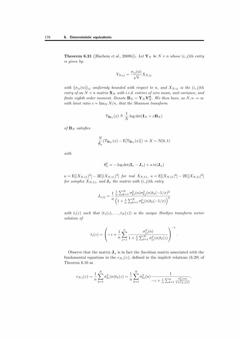
176 6. Deterministic equivalents
Theorem 6.21 ([Hachem et al., 2008b]). Let YN be N × n whose (i, j)th entry
is given by:
YN,ij =σij(n)√
nXN,ij
with {σij(n)}ij uniformly bounded with respect to n, and XN,ij is the (i, j)th
entry of an N × n matrix XN with i.i.d. entries of zero mean, unit variance, and
finite eighth order moment. Denote BN = YNYHN . We then have, as N,n→∞
with limit ratio c = limN N/n, that the Shannon transform
VBN (x) ,1
Nlog det(IN + xBN )
of BN satisfies
N
θn(VBN (x)− E[VBN (x)])⇒ X ∼ N(0, 1)
with
θ2n = − log det(In − Jn) + κ tr(Jn)
κ = E[(XN,11)4]− 3E[(XN,11)3] for real XN,11, κ = E[|XN,11|4]− 2E[|XN,11|2]
for complex XN,11, and Jn the matrix with (i, j)th entry
Jn,ij =1
n
1n
∑Nk=1 σ
2ki(n)σ2
kj(n)tk(−1/x)2(1 + 1
n
∑Nk=1 σ
2ki(n)tk(−1/x)
)2
with ti(z) such that (t1(z), . . . , tN (z)) is the unique Stieltjes transform vector
solution of
ti(z) =
−z +1
n
n∑j=1
σ2ij(n)
1 + 1n
∑Nl=1 σ
2lj(n)tl(z)
−1
.
Observe that the matrix Jn is in fact the Jacobian matrix associated with the
fundamental equations in the eN,i(z), defined in the implicit relations (6.29) of
Theorem 6.10 as
eN,i(z) =1
n
N∑k=1
σ2ki(n)tk(z) =
1
n
N∑k=1
σ2ki(n)
1
−z + 1n
∑nl=1
σ2kl(n)
1+eN,l(z)
.

6.3. A central limit theorem 177
Indeed, for all eN,k(−1/x) fixed but eN,j(−1/x), we have:
∂
∂eN,j(−1/x)
1
n
N∑k=1
σ2ki(n)
1
1x + 1
n
∑nl=1
σ2kl(n)
1+eN,l(−1/x)
=
1
n
N∑k=1
σ2ki(n)
1nσ
2kj(n)
(1 + eN,j(−1/x))2
1(1x + 1
n
∑nl=1
σ2kl(n)
1+eN,l(−1/x)
)2
=1
n
N∑k=1
1nσ
2ki(n)σ2
kj(n)tk(−1/x)2
(1 + eN,j(−1/x))2
= Jn,ji.
So far, this observation seems to generalize to all central limits derived
for random matrix models with independent entries. This is however only an
intriguing but yet unproven fact.
Similar to Theorem 3.17, [Hachem et al., 2008b] provides more than an
asymptotic central limit theorem for the Shannon transform of the information
plus noise model VBN − E[VBN ], but also the fluctuations for N large of the
difference between VBN and its deterministic equivalent VN , provided in [Hachem
et al., 2007]. In the case where XN has Gaussian entries, this takes a very compact
expression.
Theorem 6.22. Under the conditions of Theorem 6.21 with the additional
assumption that the entries of XN are complex Gaussian, we have:
N√− log det (In − Jn)
(VBN (x)− VN (x))⇒ X ∼ N(0, 1)
where VN is defined as
VN (x) =1
N
N∑i=1
log
(x
ti(−1/x)
)+
1
N
n∑j=1
log
(1 +
1
n
N∑l=1
σ2lj(n)tl(−1/x)
)
− 1
Nn
∑1≤i≤N1≤j≤n
σ2ij(n)ti(−1/x)
1 + 1n
∑Nl=1 σ
2lj(n)tl(−1/x)
with t1, . . . , tN and Jn defined as in Theorem 6.21.
The generalization to distributions of the entries of XN with a non-zero
kurtosis κ introduces an additional bias term corresponding to the limiting
variations of N(E[VBN (x)]− VN (x)). This converges instead to zero in the
Gaussian case or, as a matter of fact, in the case of any distribution with null
kurtosis.
This concludes this short section on central limit theorems for deterministic
equivalents.

178 6. Deterministic equivalents
This also closes this chapter on the classical techniques used for deterministic
equivalents, when there exists no limit to the e.s.d. of the random matrix under
study. Those deterministic equivalents are seen today as one of the most powerful
tools to evaluate the performance of large wireless communication systems
encompassing multiple antennas, multiple users, multiple cells, random codes,
fast fading channels, etc. which are studied with scrutiny in Part II. In order
to study complicated system models involving e.g. doubly-scattering channels,
multi-hop channels, random precoders in random channels, etc., the current trend
is to study nested deterministic equivalents; that is, deterministic equivalents
that account for the stochasticity of multiple independent random matrices, see
e.g. [Hoydis et al., 2011a,b].
In the following, we turn to a rather different subject and study more deeply
the limiting spectra of the sample covariance matrix model and of the information
plus noise model. For these, much more than limiting spectral densities is
known. It has especially been proved that, under some mild conditions, the
extreme eigenvalues for both models do not escape the support of the l.s.d.
and that a precise characterization of the position of some eigenvalues can be
determined. Some additional study will characterize precisely the links between
the population covariance matrix (or the information matrix) and the sample
covariance matrix (or the information plus noise matrix), which are fundamental
to address the questions of inverse problems and more precisely statistical eigen-
inference for large dimensional random matrix models. These questions are at
the core of the very recent signal processing tools, which enable novel signal
sensing techniques and (N,n)-consistent estimation procedures adapted to large
dimensional networks.
Related Documents