42 nd EUROPEAN CONGRESS OF THE REGIONAL SCIENCE ... file42 nd european congress of the regional science association dortmunnd, august 27-31, 2002 spatial effects on the aggregate demand

42 nd EUROPEAN CONGRESS OF THE REGIONAL SCIENCE ASSOCIATION DORTMUNND, AUGUST 27-31, 2002

SPATIAL EFFECTS ON THE AGGREGATE DEMAND

Fernando Barreiro-Pereira

Universidad Nacional de Educación a Distancia Faculty of Economics and Business Administration

Department of Economic Analysis C/Senda del Rey nº 11.-28040 - MADRID, Spain.

Phone:+34 913987809-Fax: +34 913986045 E-mail: [email protected]

ABSTRACT

This paper analyses if several spatial variables coming from cities and transportation system

affect money market specially the income velocity of circulation. Assuming a unit-elastic

aggregate demand function and considering money velocity as a conventional variable,

fluctuations in the velocity of circulation caused by some non-strictly economic variables, can

affect output and prices level. The empirical specification has been deduced from Baumol and

Tobin model for transaction money demand, and has the income velocity of circulation as

endogenous variable and the country’s first city population, the population density, the passenger-

kilometers transported by railways, and several ratios referred to some geographical variables, as

regressors. This model has been applied across 64 countries during the period 1978-1991. Panel

data techniques has been used for estimating the model. Estimation results indicate that most of

the explanatory variables are significant. Moreover, the another variable a part from velocity,

which affects the unit-elastic aggregate demand curve is the quantity of money in the

equilibrium, M, that we will take as a new endogenous variable for checking if the explanatory

variables of velocity can also affect the quantity of money. The equilibrium is finally affected by

these spatial variables by means of a multiplier effect, and prices and output levels maybe

influenced.

Spatial Effects on the Aggregate Demand

2

Key words : spatial variables, transportation, income velocity of circulation, panel data. JEL Class.: R-12 / L-92 / E-41 / C-33.


3

1. INTRODUCTION

Spatial issues are generally neglected in conventional macroeconomic modeling, because

the goods market is usually assumed to be in perfect competition. In fact, most spatial models

are microeconomic and do not embody the money market. Incorporating space into

macroeconomic models implies to consider product differentiation, and hence imperfect

competition in goods market, as indicate in Gabszewicz and Thisse (1980), and in Thisse

(1993). New Keynesian economics seems the framework in which space can be embodied in

macroeconomic modeling. So, real rigidities due to agglomeration economies which lead to

increasing returns to scale and hence coordination failures, together with the probable

existence of nominal frictions due to near-rationality, cost-based prices and the externalities

coming from aggregate demand fluctuations, can cause nominal rigidities and hence can

provoke that money would not be neutral because the output fluctuates, according to

Nishimura (1992). Space generates generally imperfect competition and real rigidities, but if

space could also cause some nominal frictions which provokes fluctuations in aggregate

demand, then space can be responsible of some nominal rigidities, an hence can cause

indirectly non neutrality in money. Moreover, not only there are a great difficulty to include the

space in a macroeconomic model, but also in reverse, is not still possible to introduce the

money market in a spatial microeconomic model.

The best microeconomic model which incorporates the money in a framework of

imperfect competition is the model of Blanchard an Kiyotaki (1987), which considers

monopolistic competition with product differentiation in Dixit-Stiglitz sense. In this model,

households choice between a composite good, and money. Following the Dixit-Stiglitz (1977)

approach, each household has a CES utility function because is the best form to introduce

money in the choice of consumer, and faces a usual budget constraint. The household problem

is to maximize the utility function subject to the budget constraint and, as a result of this

optimization, we will have the individual demand functions. Then, we can obtain the aggregate

demand function by aggregating these individual demands:

PM

gg

P

YPY

n

jjj

−==

∑=

11 1


4

Where Y is the real income, and g is a constant. M is money in equilibrium and P is the

prices level. This aggregate demand function is one-elastic, and reflect apparently a neo-

quantitative theory of money, where the coefficient (g/(1-g)) play the role of income velocity of

circulation (V). The parameter g is the exponent of real money balances in the CES utility

function. This microeconomic aggregate demand function has two versions in

macroeconomics: A neoclassical form, used from Fisher (1911), until Lucas (1973), where V

is considered a constant. The other version is considered in a new-keynesian framework,

basically in Blanchard, Mankiw and Corden; in this version V can be not constant. Then, if the

macroeconomic aggregate demand function considered in our problem is typically unit-elastic

such as Lucas (1973) or Corden (1980) case: P.y = M.V, fluctuations in the amount of money

(M) can affect output (y) in a Keynesian framework. In a Neoclassical framework, fluctuations

in the amount of money affect level of prices (P) only, because money velocity (V) is constant

in this model. In a conventional Keynesian model, the income velocity of circulation is not a

relevant variable because the aggregate demand function here considered is not generally unit-

elastic, and V results an erratic variable. One important question that we are worried about, is:

If income velocity of circulation is neither constant nor a erratic ratio, but it is a conventional

variable, can then V affect the output or prices? Maybe the income velocity of circulation (V)

was a variable neither so erratic as some authors say, nor a short-run constant as others say.

The fact that V was identically equal to the ratio of two macroeconomic variables such as

nominal income and the stock of money, both measured in nominal terms, means that V was

only measurable as a real figure. Surely, it should be somewhat more considered Irving

Fisher’s (1911) observation, in the sense of velocity being a variable also depending on the

state of transports and communications’ infrastructure, as well as institutional factors apart

from the well-known macroeconomic variables such as the price level, real income, the interest

rate, the inflation rate or, conversely, the stock of money. A preliminary attempt in this

analysis has been made by Mulligan and Sala i Martin (1992). These authors estimate a money

demand function using data for 48 US states covering the 1929-1990 period, where

population density was included as an additional explanatory variable. They find a significant

role for this variable in the explanation of US money demand patterns during that period.

The main aim of this paper is to analyze whether several space variables stemming from

the cities and transportation systems would affect the quantity of money demanded in the


5

equilibrium, and hence the income velocity of circulation. In this model, the income velocity of

circulation is theoretically not constant but it is a variable incorporated in some unit-elastic

aggregate demand functions such as the Corden case. We study the possible relationship

between money velocity (as a proxy for money demand), and several space variables,

fundamentally derived from the Baumol-Tobin model of transactions demand for money. The

specification of this model is in section 2 of this paper and section 3 contains an application.

Finally in section 4 there are some implications in the macroeconomic equilibrium and the

section 5 contains the conclusions.

2. THEORETICAL MODEL

In this section, we will study the possible existence of a relationship between economic

geography variables and velocity and, in such a case, to specify a model which embodying

some of the considerations made previously. As a starting point for this analysis, we will

establish some previous hypotheses. First, with the aim of simplifying the process, we will

assume that money is only demanded for transactional purposes. This restriction does not

mean any loss of generality regarding the results, and might be relaxed by including the

precautionary and speculative motives in the equation of the demand for money. Second, we

assume that money market is in equilibrium. Third, we will use as the money stock the M1

money aggregate, that is, currency in the hands of the public plus sight deposits. The

specification of the model will be based in the three following points: i) some expansion on the

Baumol-Tobin model for transaction money demand. ii)An unit-elastic aggregate demand MV,

where V is considered as a conventional variable. iii) The spatial central places theory starting

from Christaller and Lösch.

Under these assumptions, we will follow, first, the transactions demand for money

approach due to Baumol (1952) and Tobin (1956). This is a Keynesian-type approach in

which the optimum number of exchanges between bonds and money made by an individual

agent, is related with individual nominal income. Other additional restriction is given by the

consideration of a representative agent, which obtains with a monthly frequency a certain level

of nominal income (Ym). If the volume of every exchange between bonds and money is always

the same (Z) and the agent makes n exchanges, it can be said that:


6

nZ = Ym 2

The average monthly balance (m) will be in any case Z/2, and, because of that:

m = Z/2 = Ym /(2n) 3

that is, given the number of exchanges and people’s nominal income, we can know the

average money balance in nominal terms kept by the agent (m). If the nominal interest rate is r,

the opportunity cost of keeping money will be:

rm = rYm /(2n). 4

We will assume that the agents incur a fixed nominal cost (b) every time an exchange is

made. The total cost of keeping money for frequent transactions versus keeping bonds will be:

C = bn+(rYm)/(2n) 5

The number of monthly exchanges is optimum when the cost is minimum

∂C/∂n = 0 = b-(rYm)/(2n2) ⇒ n = (rYm /2b)1/2 6

and it is easy to show that second derivatives fullfil condition of minimum. The average nominal

balances that minimize the cost of maintaining money by agent and month is :

m = (bYm / 2r)1/2 7

An agent obtains an income of 12Ym per year and makes 12n exchanges. The annual

nominal average balances (ma) by individual is:

ma = 12Ym / (2(12n)) = Ym /(2n) = m 8

If we assume that the total population of the country is (PO), the total money demand

for transactions (MD) is:

MD = PO.ma = PO.m = (PO.b(12Ym.PO)/(24r))1/2 9

where (12Ym.PO) is the aggregate annual nominal income (Y). If the money market is in

equilibrium we have that MD = MS (money supply) = M(quantity of money in circulation).

The income velocity of circulation is defined as V = Y/M, and after substituting we have:

V = (24rY/PO.b)1/2 10

and separating the nominal interest rate:

V = (24(ρ + π)Y / PO.b)1/2 11

where π is the inflation rate and ρ the real interest rate. The last expression explains V as a

function of some conventional macroeconomic variables, except for PO. The total number of

optimal exchanges that the total population of the country made during a year is:

N = 12n.PO = (6rY.PO/b)1/2 12


7

and hence:

V = (24rY/(b.PO))1/2 = (2/PO)(6rY.PO/b)1/2 = 2N/ PO 13

which is a result similar to that obtained in Barro (1991). N is the total number of annual

exchanges in the country but also means the number of journeys for changing money to make

annual transactions. Perhaps there exists correlation between the number of exchanges made

within a certain area during a year, and the total number of journeys made during that time in

that area for made several transactions. These journeys are made by several transport

systems. We only consider two of them ir our model: road and railway transport but not air,

sea and walking transportation, because the impact on land of these last systems is small. At

the same time, there are, as usually passenger and freight transportation.

The application of the model which we try to specify is going to take place in the context

of the so-called metropolitan areas, in a broad sense. The basic configuration of these ones

comes from the analysis by Christaller (1933) and Lösch (1954), who in a simplified way,

infer that in the center of the area there exist a central place, which is the most important center

of population. Approximately in the middle of the central place there is the so-called central

business district, which usually includes the markets for consumption and investment goods

being the most important in that area, and where some goods non existing in any other place of

the area can be purchased. Surrounding the central place and at a certain distance, there are

usually six important, and similar, population centers, smaller than the central place. Each of

these second-order centers is surrounded by approximately six other third-order centers,

including markets for basic goods.

We consider for the analysis of the number of journeys the simplest cities system of W.

Christaller: A metropolitan area with a central place and six small similar cities around. The

Christaller’s system assumes monopolistic competition in partial equilibrium with vertical

product differentiation in Chamberlin sense. Our preference for this type of differentiation

versus the horizontal differentiation from Hotelling (1929) until Fujita and Krugman (1992) is

due to reasons of simplicity, and because there are not fall in the generality of this problem.

Following this simple model, if population of the central place is PC , and the population of

each satellite city is Pi , the number of journeys generated between central place and one

satellite city can be expressed according to a gravity model:


8

nc = β . PC.Pi / dα

14

where β and α are constants to be estimated, and (d) is the distance between cities. If we

consider that PO is the total area population, then total journeys across the center is:

Nc = 6β .PC.Pi / dα = (β/ dα)(PC.PO-(PC)2)

15

If we assume, for simplicity, that β and α are constant into the area, the transversal

journeys generated between satellite cities is:

Nt = 6β(Pi)2/dα = (β/6dα)((PO)2-2 PC.PO + (PC)2)

16

The total number of journeys generated in the area and expressed in journeys per head

will be:

Ncs /PO = (Nc + Nt)/PO = (β/6dα)((PO)2 + 4 PC.PO - 5(PC)2)

17

In the same sense, and remembering that in our model we consider only the road and

railways transportation, we can try now to calculate the number of journeys made into a

metropolitan area by both transportation systems. Following Thomas (1993), Valdés (1988)

and Button et al.(1993) for road transportation, the generation and attraction of traffic by road

is a function of cars and trucks stock and the cars / trucks ratio in the area. Considering that

the greater part of this traffic is by cars, a possible function of road traffic’s generation-

attraction is:

Nrd = k.(AUT).φ1(CAM, AUT/CAM)

18

where (Nrd) is the total number of road journeys, by cars and trucks, into the area, AUT is

cars’ stock, CAM is trucks’ stock, both in circulation, k is a constant and φ1 is a function. The

total journeys by road system per head are:

Nrd / PO = k(PC / PO)(AUT/ PC).φ1(CAM, AUT/CAM)

19

In the same way, following Izquierdo (1982), Oliveros (1983) and Friedlaender et al.(1993)

for railways transportation system , the total journeys during a year by train are dependent

basically on passenger-kilometer (PASKM) and net ton-kilometer (TNKM) carried and


9

PASKM/TNKM ratio. Passengers-kilometer is defined as the sum of kilometers traveled by

each passenger per year. Net ton-kilometer is the sum of kilometers that each ton is carried

per year. Considering that the greater part of traffic’s volume by railways are freight, a

possible function for the volume of traffic is:

Nrw = k.(TNKM).φ2(PASKM, PASKM / TNKM)

20

where (Nrw) are journeys by railway, passengers and freight, into the area during a year, k is

some constant and φ2 is a certain function. The traffic volume per inhabitant will be:

Nrw/PO = k(PC/PO)(TNKM / PC).φ2(PASKM, PASKM / TNKM)

21

The total number of journeys (Nts) due to the transportation system into the area during

a year is Nts = Nrd + N rw. In per capita terms it is expressed:

Nts/PO=λ(PC/PO)((AUT/PC).φ1(CAM,AUT/CAM)+(TNKM/PC).φ2(PASKM,

PASKM / TNKM)).

22

where λ is a parameter to be estimated. It can be useful to remember here that the total

number of journeys per capita due to the cities system was:

Ncs / PO = (µ / dα)(PO + 4PC(1-(5/4)(PC/PO)))

23

where µ is a constant. Both systems (transportation and cities) provide different variables for

explaining the same problem that is the total individual journeys made during a year within an

area. Hence, it must exist a certain probability that journeys’ explanatory variables will be a

composition, probably non linear, of these two systems.

By simplifying explanatory variable names, we will call PCPO to PC/PO; AUTPC to

AUT/PC ; AUTCAM to AUT/CAM; PKMTKM to PASKM/TNKM ; and TKMPC to

TNKM/PC. With these considerations, total journeys per head can be expressed as a

function as follows:

N*/PO = f (PO, PC, PCPO, CAM, PASKM, AUTPC, TKMPC, AUTCAM,

PKMTKM)

24


10

If there exists some correlation between the total journeys and the journeys for

exchanges between bonds an money, we will have:

N / PO = ϕ( N*/ PO)

25

but remembering equation (13): V(money velocity) = 2N / PO = 2ϕ( N*/ PO), we have the

final specification of the income velocity of circulation model as follows:

V = F (PO, PC, PCPO, CAM, PASKM, AUTPC, TKMPC, AUTCAM, PKMTKM)

26

where income velocity (V) is made dependent on the population of the main city of the

concerned country (PC), the country’s total population (PO), the ratio of PC to the country's

total population (PCPO), the number of road passenger vehicles located into the country

divided by population of country’s first city (AUTPC), the number of trucks located into the

country (CAM), the number of passenger-kilometer transported by railways (PASKM), the

passengers-kilometer/ net ton-kilometer railways ratio (PKMTKM), the cars/trucks road

ratio (AUTCAM), and the number of net ton-kilometer transported by railways divided by

population of country’s first city (TKMPC). All the variables are referred to a particular year.

3. EMPIRICAL MODEL

The specification of the theoretical model embody probably a non linear model, but

following the standard formulation of panel techniques and again for simplicity, the model

which was finally estimated was a linear one such as:

Vit=α it+µi+B1(PCPO)it+B2(PC)it+B3(PKMTKM)it+B4(AUTCAM)it+B5(PASKM)it+

+B6(AUTPC)it + B7(PO)it + B8(CAM)it + B9 (TKMPC)it + ξ it

30

where V is the endogenous variable and the rest are the explanatory variables. Although the

specification of the model according to Christaller is expected to be applied to metropolitan

areas, there exist several difficulties to collect some of the data. Specifically there are not

generally M1 data for regions and even less for metropolitan areas. Moreover, the area’s

surface do not appear into the specification of the theoretical model. In the specification of the

model, the central place theory is applied to calculate the total journeys into a metropolitan


11

area, but the total population of one country is basically the addition of the populations of all

metropolitan areas in the country. The total number of journeys made into the country are the

addition of journeys into each metropolitan area plus the journeys among these areas. Total

number of journeys in a country is a linear function of the journeys made into a metropolitan

area. These are the reasons to try the application of the model to several countries.

The variables are measured as follows: V is the ratio between GDP at market prices

and M1 monetary aggregate, both in national currency units; PC and PO are measured in

millions inhabitants; The ratio PCPO is an agglomeration index measured as 100(PC/PO); the

ratios AUTCAM and PKMTKM are directly AUT/CAM and PASKM / TNKM,

respectively; AUT and CAM are measured in thousands units; PASKM and TNKM are both

measured in millions, and AUTPC and TKMPC are directly AUT/PC and TNKM/PC

respectively. Velocity (V) and the AUTCAM and PKMTKM are real numbers; the AUTPC

ratio is measured in physical quantities divided by physical quantities, and the rest of variables

are measured in physical quantities. All variables are hence deflated.

The data set includes yearly variables for 64 countries (19 European, 17 Asian, 14

African, and 14 American), and the period of 14 years (1978 to 1991). All countries of the

sample have road and railways transportation system, and only a small group of countries with

railways transportation are excluded from the sample because of incomplete data In Figure 1,

we can observe some spatial correlation in the endogenous variable, income velocity of

circulation, among several countries as say Anselin and Florax (1995). The data are collected

basically from several sources, mainly: National Accounts Statistics, Tables 1992. United

Nations Statistical Year Book, 37-38-39 issues; United Nations. International Financial

Statistics Yearbook, (1994); International Monetary Fund. Statistical Trends in Transport,

(1965-1989); E.C.M.T. World Tables, (1991). World Bank and The Europe Year Book,

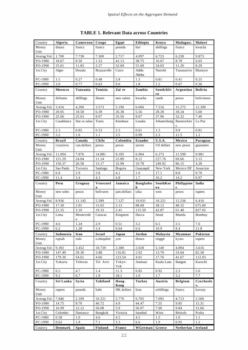
(1989). E.P.L. A group of relevant data are shown in Table 1.

The former model has been estimated using panel data techniques, following the basic

references of Hsiao (1986) and Green (1993). This is the way to take advantage when time

series data are few and control country specific heterogeneity which states constant over time.

We make the estimation using basic panel data techniques, i.e. OLS, between groups, within-

groups and GLS. Afterwards, we test the hypotheses embodied amongst these methods. First,


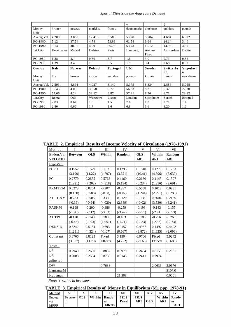
12

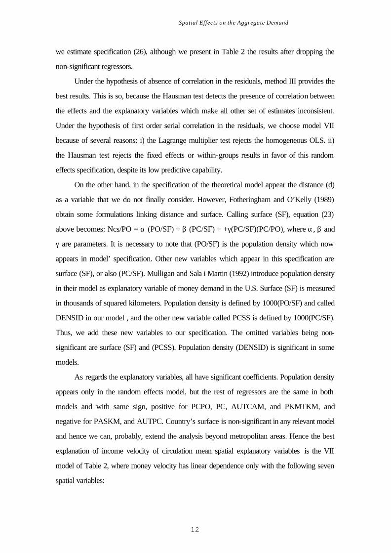
we estimate specification (26), although we present in Table 2 the results after dropping the

non-significant regressors.

Under the hypothesis of absence of correlation in the residuals, method III provides the

best results. This is so, because the Hausman test detects the presence of correlation between

the effects and the explanatory variables which make all other set of estimates inconsistent.

Under the hypothesis of first order serial correlation in the residuals, we choose model VII

because of several reasons: i) the Lagrange multiplier test rejects the homogeneous OLS. ii)

the Hausman test rejects the fixed effects or within-groups results in favor of this random

effects specification, despite its low predictive capability.

On the other hand, in the specification of the theoretical model appear the distance (d)

as a variable that we do not finally consider. However, Fotheringham and O’Kelly (1989)

obtain some formulations linking distance and surface. Calling surface (SF), equation (23)

above becomes: Ncs/PO = α (PO/SF) + β (PC/SF) + +γ(PC/SF)(PC/PO), where α, β and

γ are parameters. It is necessary to note that (PO/SF) is the population density which now

appears in model’ specification. Other new variables which appear in this specification are

surface (SF), or also (PC/SF). Mulligan and Sala i Martin (1992) introduce population density

in their model as explanatory variable of money demand in the U.S. Surface (SF) is measured

in thousands of squared kilometers. Population density is defined by 1000(PO/SF) and called

DENSID in our model , and the other new variable called PCSS is defined by 1000(PC/SF).

Thus, we add these new variables to our specification. The omitted variables being non-

significant are surface (SF) and (PCSS). Population density (DENSID) is significant in some

models.

As regards the explanatory variables, all have significant coefficients. Population density

appears only in the random effects model, but the rest of regressors are the same in both

models and with same sign, positive for PCPO, PC, AUTCAM, and PKMTKM, and

negative for PASKM, and AUTPC. Country’s surface is non-significant in any relevant model

and hence we can, probably, extend the analysis beyond metropolitan areas. Hence the best

explanation of income velocity of circulation mean spatial explanatory variables is the VII

model of Table 2, where money velocity has linear dependence only with the following seven

spatial variables:


13

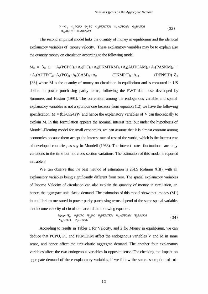
V o PCPO PC PKMTKM AUTCAM PASKMAUTPC DENSID

= + + + + + ++ +

Φ Φ Φ Φ Φ ΦΦ Φ

1 2 3 4 5

6 7 32

The second empirical model links the quantity of money in equilibrium and the identical

explanatory variables of money velocity. These explanatory variables may be to explain also

the quantity money on circulation according to the following model:

Mit = β it+µi +A1(PCPO)it+A2(PC)it+A3(PKMTKM)it+A4(AUTCAM)it+A5(PASKM)it +

+A6(AUTPC)it+A7(PO)it+A8(CAM)it+A9 (TKMPC)it+A10 (DENSID)+ξ it

33 where M is the quantity of money on circulation in equilibrium and is measured in US

dollars in power purchasing parity terms, following the PWT data base developed by

Summers and Heston (1991). The correlation among the endogenous variable and spatial

explanatory variables is not a spurious one because from equation (12) we have the following

specification: M = (b.PO/24.r)V and hence the explanatory variables of V can theoretically to

explain M. In this formulation appears the nominal interest rate, but under the hypothesis of

Mundell-Fleming model for small economies, we can assume that it is almost constant among

economies because them accept the interest rate of rest of the world, which is the interest rate

of developed countries, as say in Mundell (1963). The interest rate fluctuations are only

variations in the time but not cross-section variations. The estimation of this model is reported

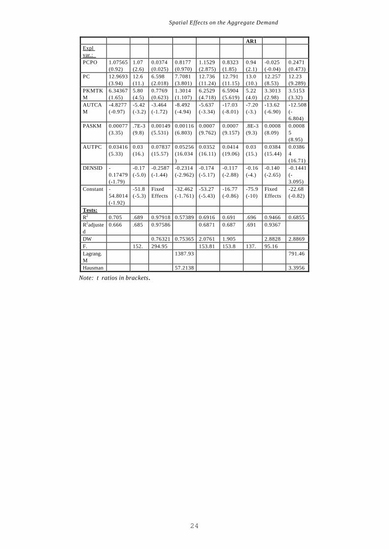
in Table 3.

We can observe that the best method of estimation is 2SLS (column XIII), with all

explanatory variables being significantly different from zero. The spatial explanatory variables

of Income Velocity of circulation can also explain the quantity of money in circulation, an

hence, the aggregate unit-elastic demand. The estimation of this model show that money (M1)

in equilibrium measured in power parity purchasing terms depend of the same spatial variables

that income velocity of circulation accord the following equation:

Mppp o PCPO PC PKMTKM AUTCAM PASKMAUTPC DENSID

= + + + + + ++ +

Ψ Ψ Ψ Ψ Ψ ΨΨ Ψ

1 2 3 4 5

6 7 34

According to results in Tables 1 for Velocity, and 2 for Money in equilibrium, we can

deduce that PCPO, PC and PKMTKM affect the endogenous variables V and M in same

sense, and hence affect the unit-elastic aggregate demand. The another four explanatory

variables affect the two endogenous variables in opposite sense. For checking the impact on

aggregate demand of these explanatory variables, if we follow the same assumption of unit-


14

elastic aggregate demand, we must estimate the relationship between monetary income, that is

the result of multiplying V and M, and all spatial explanatory variables of V and M. The

relationship among nominal income and the spatial explanatory variables is not a spurious one,

because from equation (12) we obtain the following specification: I = (b.PO/24.r)V2 where I

is the nominal income, and r is the nominal interest rate. The considerations on the nominal

interest rate are the same that in the estimation of money in equilibrium. The model is not linear

but for simplicity we will linearize in order to estimate a classic panel data model. The results of

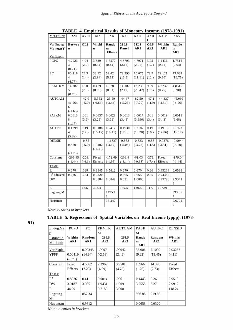
this estimation are shown in Table 4.

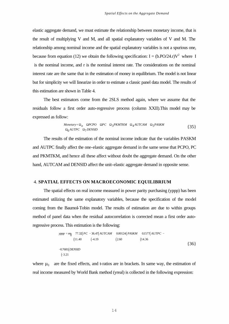
The best estimators come from the 2SLS method again, where we assume that the

residuals follow a first order auto-regressive process (column XXII).This model may be

expressed as follow:

Monetary o PCPO PC PKMTKM AUTCAM PASKMAUTPC DENSID

= + + + + + ++ +

Ω Ω Ω Ω Ω ΩΩ Ω

3 4 5

6 7 35

The results of the estimation of the nominal income indicate that the variables PASKM

and AUTPC finally affect the one-elastic aggregate demand in the same sense that PCPO, PC

and PKMTKM, and hence all these affect without doubt the aggregate demand. On the other

hand, AUTCAM and DENSID affect the unit-elastic aggregate demand in opposite sense.

4. SPATIAL EFFECTS ON MACROECONOMIC EQUILIBRIUM

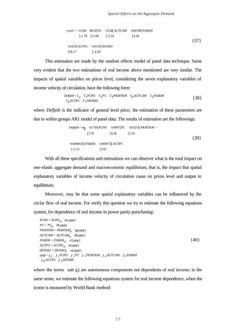
The spatial effects on real income measured in power parity purchasing (yppp) has been

estimated utilizing the same explanatory variables, because the specification of the model

coming from the Baumol-Tobin model. The results of estimation are due to within groups

method of panel data when the residual autocorrelation is corrected mean a first order auto-

regressive process. This estimation is the following:

( ) ( ) ( ) ( )( ) ( ) ( ) ( )

( )( )

yppp ij PC AUTCAM PASKM AUTPC

DENSID

= + − + + −

−

µ 77 32 36 47 0 00124 01577

0 7681

. . . .

.

11.40 -4.19 2.60 14.36

-3.21

36

where µij are the fixed effects, and t-ratios are in brackets. In same way, the estimation of

real income measured by World Bank method (yreal) is collected in the following expression:


15

( ) ( ) ( )( ) ( ) ( ) ( )

( ) ( )( ) ( )

yreal PC AUTCAM PASKM

AUTPC DENSID

= − + − + +

+ −

15194 80 51 25 56 0 00190

0 1831 10152

. . . .

. .

-1.78 13.08 -3.54 4.18

18.17 -4.59

37

This estimation are made by the random effects model of panel data technique. Same

very evident that the two estimations of real income above mentioned are very similar. The

impacts of spatial variables on prices level, considering the seven explanatory variables of

income velocity of circulation, have the following form:

Deflpib o PCPO PC PKMTKM AUTCAM PASKMAUTPC DENSID

= + + + + + ++ +

Γ Γ Γ Γ Γ ΓΓ Γ

1 2 3 4 5

6 7 38

where Deflpib is the indicator of general level price; the estimation of these parameters are

due to within groups AR1 model of panel data. The results of estimation are the followings:

( ) ( ) ( )( ) ( ) ( )

( ) ( )( ) ( )

Deflpib ij PCPO PC PKMTKM

PASKM AUTPC

= + + + −

− +

µ 01739 0 0997 0 03253

0 0000025 0 000072

. . .

. .

2.78 6.36 3.10

-2.15 3.02

39

With all these specifications and estimations we can observer what is the total impact on

one-elastic aggregate demand and macroeconomic equilibrium, that is, the impact that spatial

explanatory variables of income velocity of circulation cause on prices level and output in

equilibrium.

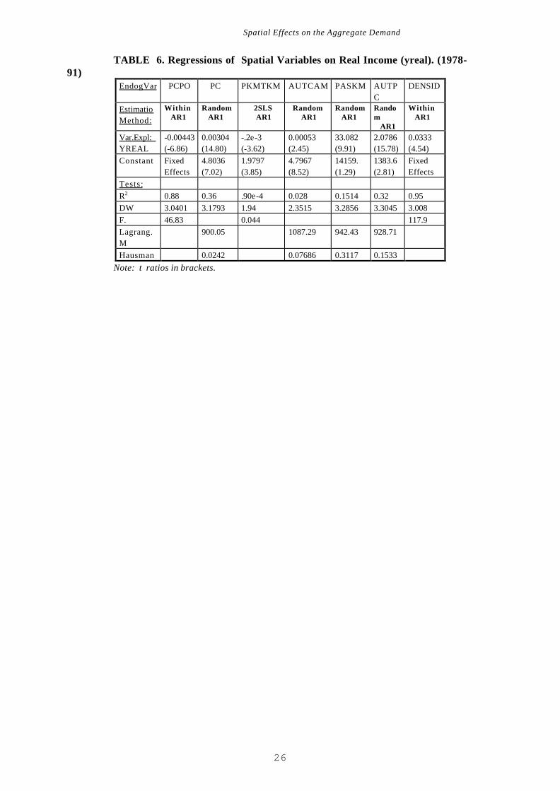
Moreover, may be that some spatial explanatory variables can be influenced by the

circlar flow of real income. For verify this question we try to estimate the following equations

system, for dependence of real income in power parity purschasing:

PCPO PCPOo ypppPC PCo ypppPKMTKM PKMTKMo ypppAUTCAM AUTCAMo ypppPASKM PASKMo ypppAUTPC AUTPCo ypppDENSID DENSID ypppyppp PCPO PC PKMTKM AUTCAM PASKM

AUTPC DENSID

= += +

= += +

= += += +

= + + + + + ++ +

α

β

γ

δ

χ

ν

ωϕ ϕ ϕ ϕ ϕ ϕ

ϕ ϕ

( )

( )

( )

( )

( )

( )

( )0

0 1 2 3 4 5

6 7

40

where the terms sub (0) are autonomous components not dependents of real income; in the

same sense, we estimate the following equations system for real income dependence, when the

icome is measured by World Bank method:


16

PCPO PCPOo yrealPC PCo yrealPKMTKM PKMTKMo yrealAUTCAM AUTCAMo yrealPASKM PASKMo yreal

AUTPC AUTPCo m yrealDENSID DENSIDo g yrealyreal o PCPO PC PKMTKM AUTCAM PASKM

AUTPC DENSID

= += +

= += +

= +

= += +

= + + + + + ++ +

λ

τ

ζ

η

π

θ θ θ θ θ θ

θ θ

( )

( )

( )

( )

( )

( )

( )

1 2 3 4 5

6 7

41

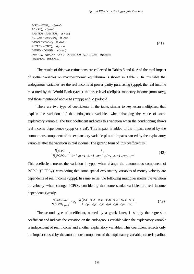
The results of this two estimations are collected in Tables 5 and 6. And the total impact

of spatial variables on macroeconomic equilibrium is shown in Table 7. In this table the

endogenous variables are the real income at power parity purchasing (yppp), the real income

measured by the World Bank (yreal), the price level (deflpib), monetary income (monetary),

and those mentioned above M (mppp) and V (velocid).

There are two type of coefficients in the table, similar to keynesian multipliers, that

explain the variations of the endogenous variables when changing the value of some

explanatory variable. The first coefficient indicates this variation when the conditioning shows

real income dependence (yppp or yreal). This impact is added to the impact caused by the

autonomous component of the explanatory variable plus all impacts caused by the explanatory

variables after the variation in real income. The generic form of this coefficient is:

( )( )∂

∂

ϕ

ϕ α ϕ β ϕ γ ϕ δ ϕ χ ϕ ν ϕ ω

yppp

PCPOo=

− − − − − − −1

1 2 3 4 5 6 71 42

This coeficcient means the variation in yppp when change the autonomous component of

PCPO, (PCPO0), considering that some spatial explanatory variables of money velocity are

dependents of real income (yppp). In same sense, the following multiplier means the variation

of velocity when change PCPO0, considering that some spatial variables are real income

dependents (yreal):

( )( )

( )∂

∂

θ λ τ ζ η π

θ λ θ τ θ ζ θ η θ π θ θ

VELOCIDPCPO

m gm go yreal

= ++ + + + + +

− − − − − − −Φ

Φ Φ Φ Φ Φ Φ Φ1

1 1 2 3 4 5 6 7

1 2 3 4 5 6 71 43

The second type of coefficient, named by a greek letter, is simply the regression

coefficient and indicate the variation on the endogenous variable when the explanatory variable

is independent of real income and another explanatory variables. This coefficient reflects only

the impact caused by the autonomous component of the explanatory variable, caeteris paribus


17

another explanatory variables and real income. How significant are these coefficients are

measured by means of the t-ratios, in brackets in this table 7.

5. CONCLUDING REMARKS

In this paper I have specified a model which links the income velocity of circulation and

some geographical variables. The model is constructed assuming a unielastic aggregate

demand function which contains the income velocity of circulation as conventional variable.

The central point of the theoretical specification was the Baumol-Tobin model for transaction

money demand. The connections with the Spatial Economy come from basically of

Christaller’s central place theory and some gravity models for the transportation system. The

model is estimated using panel data techniques for a sample of 64 countries during 14 years.

The best results are obtained in the random effects model making a correction by assuming a

first order auto-regresive process in the residuals. We have found a positive relationship

between the income velocity of circulation and the ratio between central place and total

country’ population, the ratio between cars and trucks stock in the country, the ratio between

passenger-kilometer and net ton-kilometer transported by railways into the country and finally

the central place population in absolute terms. We also have found a negative relationship

among income velocity of circulation and the passenger-kilometer transported by railways in

absolute terms, and the ratio between cars’ stock and central place population. The

regression coefficients show the variation of the income velocity of circulation when fluctuating

each explanatory variable; and hence, the income velocity of circulation increases when

increasing the conditionings whose coefficients are positive like the ratio between central place

and total country’s population (PCPO), the ratio between cars and trucks stock (AUTCAM),

the ratio between passenger-kilometer and net ton-kilometer transported by railways

(PKMTKM), the central place population (PC) and the population’s density (DENSID), or

when decreasing the explanatory variables whose coefficients are negative, i.e., the passenger-

kilometer in absolute terms transported by railways (PASKM) and, the ratio between cars’

stock and central place population (AUTPC). The variables PCPO, PC and PKMTKM

affect the total aggregate demand in same sense causing fluctuations in output and prices level,

that are cause of nominal friction. If the variables DENSID and AUTCAM coming down, or


18

rise the another spatial explanatory variables, then output also rise. Fluctuations in PCPO and

PKMTKM not affect the output. Prices level rise if PASKM come down or the another

spatial variables goes up. Fluctuations in DENSID and AUTCAM not affect the prices level.

If the spatial explanatory variables are income dependents, impacts on output are the same

that if not are income dependents. Moreover in this case, if rise AUTCAM or DENSID, or

coming down AUTPC, then prices level come down. Space apparently affect the economic

equilibrium and maybe a cause of non neutrality in money market.

________________

Acknowledgements

I am very grateful to Masayuki Sekine, Kennett Button, Luigi F. Signorini, Maurice Catin,

Kevin O’Connor, David Pitfield, Francisco Mochón, and Jose Mª Labeaga for several

comments and suggestions to a previous version of this paper. The usual disclaimer applies.

REFERENCES

Anselin, L. & R. Florax., 1995, (eds.), New Directions in Spatial Econometrics,

Spr.Verlag

Barro, R., 1991, Macroeconomía, Alianza Universidad, Madrid.

Baumol, W. J., 1952, “The Transactions Demand for Cash: An Inventory Theoretic

Approach”, Quarterly Journal of Economics , vol 66.

Blanchard, O.& N.Kiyotaki , 1987, “Monopolistic Competition and the Effects of

Aggregate Demand”, American Economic Review. vol 77.

Button, K. et al., 1993, “Modelling Vehicle Ownership and Use in Low Income Countries”,

Journal of Transport Economics and Policy.

Christaller, W.,1933, Central places in Southern Germany, ed. (1966) Prentice-Hall.

Corden, W.M ., 1980, Politique Commerciale et Bien-Être Economique, Economica. Paris

Dixit, A., and J.Stiglitz, 1977, “Monopolístic Competition and Optimum Product

Diversity”, American Economic Review, vol. 67, no 3, 297-308.

Fisher, I., 1911, The Purchasing Power of Money. New York. Macmillan.

Fotheringham, A.S.& M.E.O´Kelly, 1989, Spatial Interaction Models:Formulations and

Applications. Kluwer Acad. Publish. Dordrecht.


19

Friedlaender, A. et al., 1993, “Rail Cost and Capital Adjustments in a Quasi-Regulated

Environment”, Journal of Transport Ec. and Policy.

Fujita,M. & P.Krugman, 1992, “A Monopolistic Competition Model of Urban Systems

and Trade”, Dep.of Regional Sc.,Univ. of Penn.

Gabszewicz, J. J. & J.F. Thisse, 1980, “Entry and Exit in a Differentiated Industry”,

Journal of EconomicTheory.

Green, W., 1995, Econometric Analysis, Macmillan. New York.

Hotelling, H ., 1929, “Stability in Competition”, Economic Journal. vol 39.

Hsiao, Ch., 1986, Analysis of Panel Data , Cambridge University Press. Mass.

Izquierdo, R., 1982, La Economía del Transporte, E.T.S. de Ingenieros de C.C. y

P.Madrid

Lösch , A., 1954, The Economics of Location, New Haven,Conn..

Lucas, Jr. Robert E., 1973, “Some International Evidence on Output-Inflation Tradeoffs”,

The American Economic Review, vol 63 no.3.

Mulligan, C. & X. Sala i Martin, 1992, “US Money Demand: Surprising Cross-

sectional Estimates”, Brookings Papers on Econ. Activity.

Mundell, R.,1963, “Capital Mobility and Stabilization Policy under Fixed an Flexible

Echange Rates”, Canadian Journal of Economie.and Political Science, vol 29.

Nishimura, K., 1992, Imperfect Competition, Differential Information, and

Microfoundations of Macroeconomics,Clarendon Press, Oxford.

Oliveros, F . et al., 1983, Tratado de Explotacion de Ferrocarriles, Rueda. Madrid.

Summers, R. and A.Heston, 1991, “The Penn World Table (Mark 5): An Expanded Set

of International Comparisons, 1950-1988”, The Quarterly Journal of Economics, May.

Thisse, J. F ., 1993, “Oligopoly and the Polarization of Space”, European Economic

Review.

Thomas, R., 1993, Traffic. Assignment Techniques, Averbury Technical, Aldershot

Tobin, J., 1956, “The Interes Elasticity of Transactions Demand for Cash”, Review of

Economic Studies, vol 25.

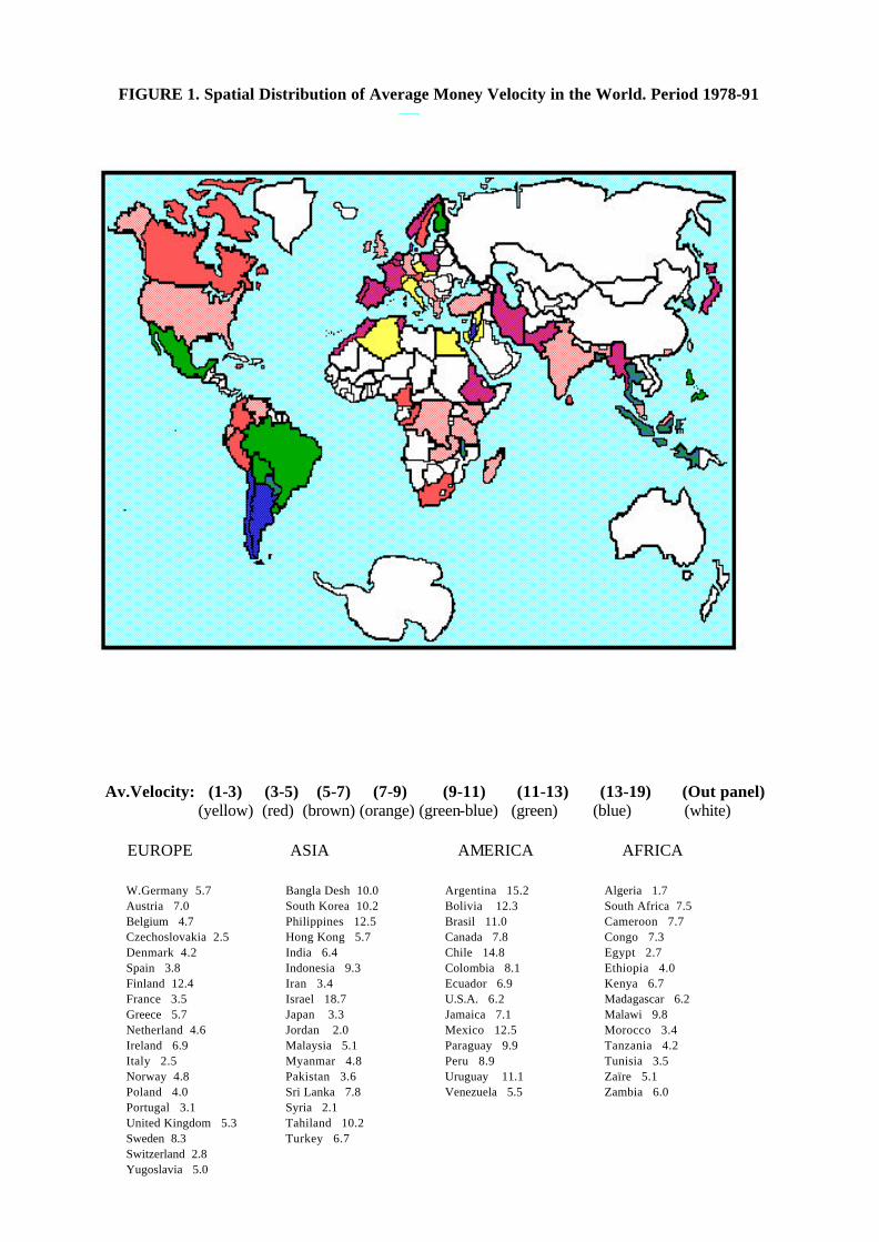
FIGURE 1. Spatial Distribution of Average Money Velocity in the World. Period 1978-91

Av.Velocity: (1-3) (3-5) (5-7) (7-9) (9-11) (11-13) (13-19) (Out panel) (yellow) (red) (brown) (orange) (green-blue) (green) (blue) (white) EUROPE ASIA AMERICA AFRICA

W.Germany 5.7 Bangla Desh 10.0 Argentina 15.2 Algeria 1.7 Austria 7.0 South Korea 10.2 Bolivia 12.3 South Africa 7.5 Belgium 4.7 Philippines 12.5 Brasil 11.0 Cameroon 7.7 Czechoslovakia 2.5 Hong Kong 5.7 Canada 7.8 Congo 7.3 Denmark 4.2 India 6.4 Chile 14.8 Egypt 2.7 Spain 3.8 Indonesia 9.3 Colombia 8.1 Ethiopia 4.0 Finland 12.4 Iran 3.4 Ecuador 6.9 Kenya 6.7 France 3.5 Israel 18.7 U.S.A. 6.2 Madagascar 6.2 Greece 5.7 Japan 3.3 Jamaica 7.1 Malawi 9.8 Netherland 4.6 Jordan 2.0 Mexico 12.5 Morocco 3.4 Ireland 6.9 Malaysia 5.1 Paraguay 9.9 Tanzania 4.2 Italy 2.5 Myanmar 4.8 Peru 8.9 Tunisia 3.5 Norway 4.8 Pakistan 3.6 Uruguay 11.1 Zaïre 5.1 Poland 4.0 Sri Lanka 7.8 Venezuela 5.5 Zambia 6.0 Portugal 3.1 Syria 2.1 United Kingdom 5.3 Tahiland 10.2 Sweden 8.3 Turkey 6.7 Switzerland 2.8 Yugoslavia 5.0


21


22

TABLE 1. Relevant Data across Countries

Country Algeria Cameroon Congo Egypt Ethiopia Kenya Madagasc. Malawi Money Unit

dinars francs francs pounds birr shillings francs kwacha

Averag.Vel. 1.700 7.738 7.300 2.717 4.097 6.723 6.238 9.873 PO-1980 18.67 8.50 1.53 42.13 38.75 16.67 8.78 6.05 PO-1990 25.01 11.83 2.27 52.69 51.69 24.03 11.20 8.29 1st.City Alger Douala Brazzaville Cairo Addis

Abeba Nairobi Tananarive Blantyre

PC-1980 1.5 0.27 0.48 5.8 1.3 0.81 0.41 0.25 PC-1990 3.0 0.77 0.63 9.0 1.8 1.5 0.67 0.36

Country Morocco Tanzania Tunisia Zaïre Zambia SouthAfrica

Argentina Bolivia

Money Unit

dirhams shillings dinars new zaïres kwacha rands pesos bolivianos

Averag.Vel. 3.416 4.200 3.573 5.190 6.066 7.516 15.272 12.390 PO-1980 20.05 18.58 6.39 26.38 5.56 28.28 28.24 5.60 PO-1990 25.06 25.63 8.07 35.56 8.07 37.96 32.32 7.40 1st.City Casablanca Dar es salaa Tunis Kinshasa Lusaka Johanesburg BuenosAire

s La Paz

PC-1980 2.3 0.85 0.53 2.5 0.61 1.5 9.9 0.81 PC-1990 3.2 1.6 1.1 3.5 0.99 2.3 11.5 1.2

Country Brazil Canada Chile Colombia Ecuador U.S.A. Mexico Paraguay Money Unit

cruzeiros can.dollars pesos pesos sucres US dollars new pesos guaranies

Averag.Vel. 11.004 7.876 14.881 8.185 6.904 6.273 12.599 9.981 PO-1980 121.29 24.04 11.14 25.89 8.12 227.76 69.66 3.15 PO-1990 150.37 26.58 13.17 32.99 10.78 249.92 86.15 4.28 1st.City Sao Paulo Toronto Santiago Bogota Guayaquil New York Mexico DF Asuncion PC-1980 6.9 2.9 3.8 4.1 1.0 17.1 8.8 0.70 PC-1990 11.4 3.4 4.3 4.8 1.7 16.2 14.2 0.97

Country Peru Uruguay Venezuela

Jamaica Bangladesh

SouthKorea

Philippines

India

Money Unit

new soles pesos bolivares jam.dollars taka won pesos rupees

Averag.Vel. 8.936 11.145 5.589 7.127 10.031 10.221 12.536 6.410 PO-1980 17.30 2.91 15.02 2.13 88.68 38.12 48.32 675.00 PO-1990 21.55 3.10 19.33 2.41 115.59 42.87 61.48 827.05 1st.City Lima Montevide

o Caracas Kingston Dacca Seoul Manila Bombay

PC-1980 4.6 1.24 2.9 0.51 3.2 6.5 3.5 7.6 PC-1990 6.2 1.28 3.4 0.64 6.6 10.9 8.4 11.8

Country Indonesia Iran Israel Japan Jordan Malaysia Myanmar Pakistan Money Unit

rupiah rials n.sheqalim yen dinars ringgit kyats rupees

Averag.Vel. 9.392 3.452 18.739 3.380 2.028 5.140 4.894 3.616 PO-1980 147.49 39.30 3.88 116.81 2.92 13.70 33.64 82.58 PO-1990 179.30 54.61 4.66 123.54 4.01 17.76 41.67 112.03 1st.City Yakarta Teheran Tel Aviv Tokyo-

Yok Amman Kuala Lum. Rangun Karachi

PC-1980 6.5 4.7 1.4 11.3 0.85 0.92 2.3 5.0 PC-1990 9.2 6.7 1.8 18.1 1.0 1.7 3.2 7.7

Country Sri Lanka Syria Tahiland Hong-Kong

Turkey Austria Belgium Czechoslov.

Money Unit

rupees pounds baht HK dollars liras schillings francs koruny

Averag.Vel. 7.846 2.109 10.221 5.770 6.705 7.095 4.713 2.500 PO-1980 14.75 8.70 46.72 4.9 44.47 7.55 9.85 15.31 PO-1990 16.99 12.12 56.08 5.9 56.07 7.60 9.84 15.66 1st.City Colombo Damasco Bangkok Victoria Istanbul Wien Brüxels Praha PC-1980 0.58 1.0 4.6 4.5 4.5 1.5 1.0 1.1 PC-1990 0.62 1.8 7.1 5.3 6.6 1.9 0.95 1.2

Country Denmark Spain Finland France WGerman Greece Netherlan Ireland


23

y d Money Unit

kroner pesetas markkaa francs deuts.marks drachmas guilders pounds

Averag.Vel. 4.200 3.868 12.413 3.586 5.728 5.784 4.684 6.992 PO-1980 5.12 37.54 4.78 53.88 61.54 9.64 14.14 3.40 PO-1990 5.14 38.96 4.99 56.73 63.23 10.12 14.95 3.50 1st.City Kφbenhavn Madrid Helsinki Paris Hamburg Atenas-

Pireo Amsterdam Dublin

PC-1980 1.38 3.1 0.80 8.7 1.6 3.0 0.71 0.86 PC-1990 1.39 3.4 1.0 8.5 1.9 3.4 0.68 0.93

Country Italy Norway Poland Portugal U.K. Sweden Switzerland

Yugoslavia

Money Unit

lire kroner zlotys escudos pounds kronor francs new dinars

Averag.Vel. 2.593 4.891 4.027 3.140 5.375 8.334 2.886 5.058 PO-1980 56.43 4.09 35.58 9.77 56.33 8.31 6.32 22.30 PO-1990 57.66 4.24 38.12 9.87 57.41 8.56 6.71 23.82 1st.City Roma Oslo Warszawa Lisboa London Stockhölm Zürich Beograd PC-1980 2.83 0.64 1.5 1.5 7.6 1.3 0.71 1.4 PC-1990 2.80 0.66 1.7 1.6 6.8 1.6 1.20 1.6

TABLE 2. Empirical Results of Income Velocity of Circulation (1978-1991) Method: I II III IV V VI VII Endog.Var VELOCID

Between OLS Within Random OLS AR1

Within AR1

Random AR1

Expl.Var: PCPO 0.1552

(3.199) 0.1529 (11.22)

0.1109 (1.797)

0.1293 (3.621)

0.1540 (10.41)

0.1270 (4.896)

0.1283 (5.630)

PC 0.2779 (1.921)

0.2885 (7.202)

0.5763 (4.818)

0.4160 (5.134)

0.2630 (6.234)

0.1145 (1.856)

0.1507 (2.691)

PKMTKM 0.0273 (0.160)

0.0264 (0.588)

-0.207 (-0.38)

-0.397 (-0.07)

0.5558 (1.244)

0.1018 (2.291)

0.0981 (2.289)

AUTCAM -0.783 (-0.39)

-0.505 (-0.94)

0.3339 (4.020)

0.2120 (2.889)

-0.135 (-0.02)

0.2604 (3.530)

0.2165 (3.241)

PASKM -0.198 (-1.98)

-0.200 (-7.12)

-0.386 (-3.33)

-0.259 (-3.47)

-0.193 (-6.51)

-0.143 (-2.91)

-0.155 (-3.53)

AUTPC -0.120 (-0.43)

-0.148 (-1.93)

0.1883 (1.051)

-0.163 (-1.21)

-0.186 (-2.33)

-0.256 (-2.38)

-0.268 (-2.73)

DENSID 0.5242 (1.231)

0.5154 (4.324)

-0.693 (-1.07)

0.2157 (0.667)

0.4967 (3.872)

0.4497 (1.825)

0.4402 (2.093)

Constant 3.8766 (3.307)

3.8123 (11.79)

Fixed Effects

3.1304 (4.222)

6.0706 (27.65)

Fixed Effects

5.9242 (5.688)

Tests: R2 0.2940 0.2630 0.8837 0.0979 0.2484 0.8159 0.2081 R2-adjusted

0.2008 0.2564 0.8730 0.0145 0.2411 0.7974

DW 0.7638 2.0636 2.0676 Lagrang.M 2107.0 Hausman 21.508 0.0001

Note: t ratios in brackets.

TABLE 3. Empirical Results of Money in Equilibrium (M1 ppp. 1978-91) Method VIII IX X XI XII XIII XIV XV XVI Endog var: MPPP

Between

OLS Within Random Effects

2SLS Panel

2SLS AR1

OLS AR1

Within AR1

Random AR1


24

AR1 Expl var.:

PCPO 1.07565 (0.92)

1.07 (2.6)

0.0374 (0.025)

0.8177 (0.970)

1.1529 (2.875)

0.8323 (1.85)

0.94 (2.1)

-0.025 (-0.04)

0.2471 (0.473)

PC 12.9693 (3.94)

12.6 (11.)

6.598 (2.018)

7.7081 (3.801)

12.736 (11.24)

12.791 (11.15)

13.0 (10.)

12.257 (8.53)

12.23 (9.289)

PKMTKM

6.34367 (1.65)

5.80 (4.5)

0.7769 (0.623)

1.3014 (1.107)

6.2529 (4.718)

6.5904 (5.619)

5.22 (4.0)

3.3013 (2.98)

3.5153 (3.32)

AUTCAM

-4.8277 (-0.97)

-5.42 (-3.2)

-3.464 (-1.72)

-8.492 (-4.94)

-5.637 (-3.34)

-17.03 (-8.01)

-7.20 (-3.)

-13.62 (-6.90)

-12.508 (-6.804)

PASKM 0.00077 (3.35)

.7E-3 (9.8)

0.00149 (5.531)

0.00116 (6.803)

0.0007 (9.762)

0.0007 (9.157)

.8E-3 (9.3)

0.0008 (8.09)

0.00085 (8.95)

AUTPC 0.03416 (5.33)

0.03 (16.)

0.07837 (15.57)

0.05256 (16.034)

0.0352 (16.11)

0.0414 (19.06)

0.03 (15.)

0.0384 (15.44)

0.03864 (16.71)

DENSID -0.17479 (-1.79)

-0.17 (-5.0)

-0.2587 (-1.44)

-0.2314 (-2.962)

-0.174 (-5.17)

-0.117 (-2.88)

-0.16 (-4.)

-0.140 (-2.65)

-0.1441 (-3.095)

Constant -54.8014 (-1.92)

-51.8 (-5.3)

Fixed Effects

-32.462 (-1.761)

-53.27 (-5.43)

-16.77 (-0.86)

-75.9 (-10)

Fixed Effects

-22.68 (-0.82)

Tests: R2 0.705 .689 0.97918 0.57389 0.6916 0.691 .696 0.9466 0.6855 R2adjusted

0.666 .685 0.97586 0.6871 0.687 .691 0.9367

DW 0.76321 0.75365 2.0761 1.905 2.8828 2.8869 F. 152. 294.95 153.81 153.8 137. 95.16 Lagrang.M

1387.93 791.46

Hausman 57.2138 3.3956



25

TABLE 4. Empirical Results of Monetary Income. (1978-1991)

Met.Estim: XVII XVIII XIX XX XXI XXII XXIII

XXIV XXV

Var.Endog: MonetarY

Between

OLS Within

Random Effects

2SLS Panel

2SLS AR1

OLS AR1

Within AR1

Random AR1

Var.Expl: PCPO 4.2023

3 (0.71)

4.04 (2.0)

3.339 (0.54)

1.7577 (0.44)

4.3703 (2.17)

4.7071 (2.01)

3.95 (1.7)

1.2436 (0.41)

1.7515 (0.64)

PC 80.1184 (4.77)

79.3 (14.)

38.92 (2.84)

52.42 (5.62)

79.293 (13.9)

70.075 (11.11)

79.9 (12.)

72.121 (9.60)

73.684 (10.75)

PKMTKM 14.3825 (0.73)

13.0 (2.0)

0.479 (0.09)

1.578 (0.31)

14.107 (2.12)

13.238 (2.042)

9.99 (1.5)

4.2232 (0.75)

4.8516 (0.90)

AUTCAM -41.9646 (-1.66)

-42.0 (-5.0)

-5.582 (-0.66)

-25.59 (-3.44)

-44.47 (-5.26)

-82.59 (-7.20)

-47.1 (-4.9)

-44.337 (-4.54)

-45.099 (-4.96)

PASKM 0.00138 (1.17)

.001 (3.5)

0.0037 (3.28)

0.0028 (3.55)

0.0013 (3.48)

0.0017 (3.896)

.001 (3.4)

0.0019 (3.43)

0.0018 (3.68)

AUTPC 0.18994 (5.82)

0.19 (17.)

0.3188 (15.15)

0.2417 (16.11)

0.1930 (17.6)

0.2182 (18.28)

0.19 (16.)

0.19155 (14.86)

0.1923 (16.17)

DENSID -0.86011 (-1.73)

-0.85 (-5.0)

-1.0402 (-1.38)

-1.1827 (-3.12)

-0.858 (-5.08)

-0.833 (-3.75)

-0.86 (-4.5)

-0.9276 (-3.31)

-0.9044 (-3.70)

Constant -209.95 (-1.44)

-203. (-4.1)

Fixed Effects

-171.69 (-1.96)

-203.4 (-4.14)

-61.03 (-0.68)

-272. (-7.4)

Fixed Effects

-179.04 (-1.44)

Tests: R2 0.678 .668 0.9845 0.5613 0.670 0.670 0.66 0.95269 0.6598 R2-adjusted 0.636 .663 0.9820 0.665 0.665 0.65 0.94386 DW 0.8884 0.8849 0.321 1.8803 2.93796 2.9341

8 F. 138. 398.4 139.5 139.5 117. 107.91 Lagrang.M 1495.1

1 893.05

4 Hausman 38.247 0.6704

9

Note: t- ratios in brackets.

TABLE 5. Regressions of Spatial Variables on Real Income (yppp). (1978-91)

Endog.Var

PCPO PC PKMTKM

AUTCAM PASKM

AUTPC DENSID

Estimatio Method:

Within AR1

Random AR1

2SLS AR1

2SLS AR1

Random AR1

Random AR1

Within AR1

Var.Expl: YPPP

-0.00419 (-5.71)

0.00345 (14.94)

-.0007 (-2.68)

.00042 (2.49)

35.006 (9.22)

2.1090 (13.45)

0.03267 (4.11)

Constant Fixed Effects

4.6862 (7.23)

2.3969 (4.69)

3.9501 (4.73)

13966. (1.26)

1414.6 (2.73)

Fixed Effects

Tests: R2 0.8826 0.41 0.0014 .0061 0.1443 0.26 0.9518 DW 3.0187 3.085 1.9431 1.909 3.2555 3.27 2.9912 F. 44.99 0.7159 3.000 118.24 Lagrang.M

857.34 936.88 919.65

Hausman 0.9812 0.0658 0.0320



26

TABLE 6. Regressions of Spatial Variables on Real Income (yreal). (1978-91)

EndogVar PCPO PC PKMTKM AUTCAM PASKM AUTPC

DENSID

Estimatio Method:

Within AR1

Random AR1

2SLS AR1

Random AR1

Random AR1

Random AR1

Within AR1

Var.Expl: YREAL

-0.00443 (-6.86)

0.00304 (14.80)

-.2e-3 (-3.62)

0.00053 (2.45)

33.082 (9.91)

2.0786 (15.78)

0.0333 (4.54)

Constant Fixed Effects

4.8036 (7.02)

1.9797 (3.85)

4.7967 (8.52)

14159. (1.29)

1383.6 (2.81)

Fixed Effects

Tests: R2 0.88 0.36 .90e-4 0.028 0.1514 0.32 0.95 DW 3.0401 3.1793 1.94 2.3515 3.2856 3.3045 3.008 F. 46.83 0.044 117.9 Lagrang.M

900.05 1087.29 942.43 928.71

Hausman 0.0242 0.07686 0.3117 0.1533


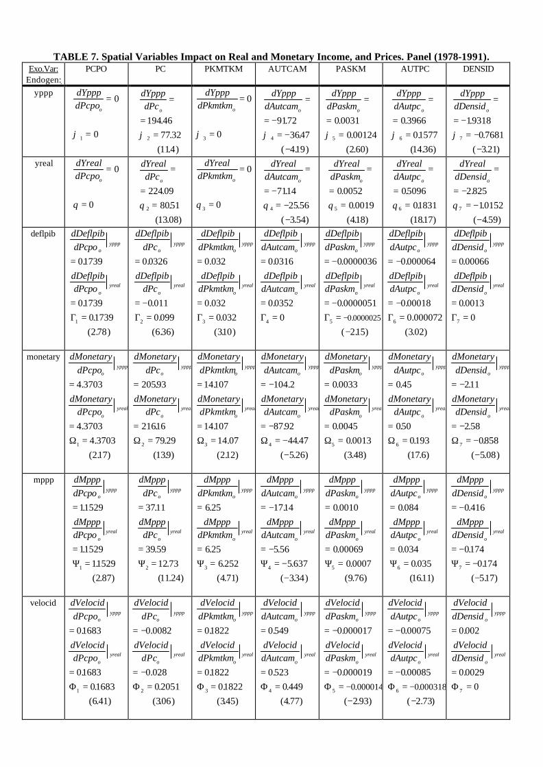
TABLE 7. Spatial Variables Impact on Real and Monetary Income, and Prices. Panel (1978-1991). Exo.Var:

Endogen: PCPO

PC PKMTKM AUTCAM PASKM AUTPC DENSID

yppp dYpppdPcpoo

=

=

0

01ϕ

dYpppdPco

=

==

194 46

77 32

1142

.

.

( . )

ϕ

dYpppdPkmtkmo

=

=

0

03ϕ

dYpppdAutcamo

=

= −= −

−

9172

3647

4194

.

.

( . )

ϕ

dYpppdPaskmo

=

==

0 0031

0 00124

2 605

.

.

( . )

ϕ

dYpppdAutpco

=

==

0 3966

01577

14 366

.

.

( . )

ϕ

dYpppdDensido

=

= −= −

−

19318

0 7681

3 217

.

.

( . )

ϕ

yreal dYrealdPcpoo

=

=

0

0θ

dYrealdPco

=

==

224 09

8051

13 082

.

.

( . )

θ

dYrealdPkmtkmo

=

=

0

03θ

dYrealdAutcamo

=

= −= −

−

7114

25 56

3 544

.

.

( . )

θ

dYrealdPaskmo

=

==

0 0052

0 0019

4185

.

.

( . )

θ

dYrealdAutpco

=

==

05096

01831

18176

.

.

( . )

θ

dYrealdDensido

=

= −= −

−

2 825

10152

4 597

.

.

( . )

θ

deflpib dDeflpibdPcpo

dDeflpibdPcpo

oyppp

oyreal

=

==

01739

01739

01739

2 781

.

.

.

( . )

Γ

dDeflpibdPc

dDeflpibdPc

oyppp

oyreal

=

= −=

0 0326

0 011

0 099

6 362

.

.

.

( . )

Γ

dDeflpibdPkmtkm

dDeflpibdPkmtkm

oyppp

oyreal

=

==

0 032

0 032

0 032

3103

.

.

.

( . )

Γ

dDeflpibdAutcam

dDeflpibdAutcam

oyppp

oyreal

=

==

0 0316

0 0352

04

.

.

Γ

dDeflpibdPaskm

dDeflpibdPaskm

oyppp

oyreal

= −

= −=

−−

0 0000036

0 0000051

2155 0 0000025

.

.

( . )

.Γ

dDeflpibdAutpc

dDeflpibdAutpc

oyppp

oyreal

= −

= −=

0 000064

0 00018

0 000072

3 026

.

.

.

( . )

Γ

dDeflpibdDensid

dDeflpibdDensid

oyppp

oyreal

=

==

0 00066

0 0013

07

.

.

Γ

monetary dMonetarydPcpo

dMonetarydPcpo

oyppp

oyreal

=

==

4 3703

4 3703

4 3703

2171

.

.

.

( . )

Ω

dMonetarydPc

dMonetarydPc

oyppp

oyreal

=

==

20593

21616

79 29

1392

.

.

.

( . )

Ω

dMonetarydPkmtkm

dMonetarydPkmtkm

oyppp

oyreal

=

==

14107

14107

14 07

2123

.

.

.

( . )

Ω

dMonetarydAutcam

dMonetarydAutcam

oyppp

oyreal

= −

= −= −

−

104 2

87 92

44 47

5 264

.

.

.

( . )

Ω

dMonetarydPaskm

dMonetarydPaskm

oyppp

oyreal

=

==

0 0033

0 0045

0 0013

3 485

.

.

.

( . )

Ω

dMonetarydAutpc

dMonetarydAutpc

oyppp

oyreal

=

==

0 45

050

0193

17 66

.

.

.

( . )

Ω

dMonetarydDensid

dMonetarydDensid

oyppp

oyreal

= −

= −= −

−

211

2 58

0858

5 087

.

.

.

( . )

Ω

mppp dMppp

dPcpo

dMpppdPcpo

oyppp

oyreal

=

==

11529

11529

11529

2 871

.

.

.

( . )

Ψ

dMpppdPc

dMpppdPc

oyppp

oyreal

=

==

3711

39 59

12 73

11 242

.

.

.

( . )

Ψ

dMpppdPkmtkm

dMpppdPkmtkm

oyppp

oyreal

=

==

6 25

6 25

6 252

4 713

.

.

.

( . )

Ψ

dMpppdAutcam

dMpppdAutcam

oyppp

oyreal

= −

= −= −

−

1714

5 56

5 637

3344

.

.

.

( . )

Ψ

dMpppdPaskm

dMpppdPaskm

oyppp

oyreal

=

==

0 0010

0 00069

0 0007

9 765

.

.

.

( . )

Ψ

dMpppdAutpc

dMpppdAutpc

oyppp

oyreal

=

==

0 084

0 034

0 035

16116

.

.

.

( . )

Ψ

dMpppdDensid

dMpppdDensid

oyppp

oyreal

= −

= −= −

−

0 416

0174

0174

5177

.

.

.

( . )

Ψ

velocid dVelociddPcpo

dVelociddPcpo

oyppp

oyreal

=

==

01683

01683

01683

6 411

.

.

.

( . )

Φ

dVelociddPc

dVelociddPc

oyppp

oyreal

= −

= −=

0 0082

0 028

0 2051

3062

.

.

.

( . )

Φ

dVelociddPkmtkm

dVelociddPkmtkm

oyppp

oyreal

=

==

01822

01822

01822

3453

.

.

.

( . )

Φ

dVelociddAutcam

dVelociddAutcam

oyppp

oyreal

=

==

0 549

0 523

0 449

4 774

.

.

.

( . )

Φ

dVelociddPaskm

dVelociddPaskm

oyppp

oyreal

= −

= −=

−−

0 000017

0 000019

2 935 0 000014

.

.

( . )

.Φ

dVelociddAutpc

dVelociddAutpc

oyppp

oyreal

= −

= −=

−−

0 00075

0 00085

2 736 0000318

.

.

( . )

.Φ

dVelociddDensid

dVelociddDensid

oyppp

oyreal

=

==

0 002

0 0029

07

.

.

Φ

42 nd EUROPEAN CONGRESS OF THE REGIONAL SCIENCE ... file42 nd european congress of the regional science association dortmunnd, august 27-31, 2002 spatial effects on the aggregate demand

Documents