4. Random Variables - Statisticsdept.stat.lsa.umich.edu/~ionides/425/notes/random_variables.pdf · 4. Random Variables • Many random processes produce numbers. These numbers are

4. Random Variables

• Many random processes produce numbers.These numbers are called random variables.

Examples

(i) The sum of two dice.

(ii) The length of time I have to wait at the busstop for a #2 bus.

(iii) The number of heads in 20 flips of a coin.

Definition. A random variable, X, is afunction from the sample space S to the realnumbers, i.e., X is a rule which assigns a numberX(s) for each outcome s ∈ S.Example. For S = {(1, 1), (1, 2), . . . , (6, 6)} therandom variable X corresponding to the sum isX(1, 1) = 2, X(1, 2) = 3, and in generalX(i, j) = i + j.

Note. A random variable is neither random nor avariable. Formally, it is a function defined on S.

1

Defining events via random variables

• Notation: we write X = x for the event{s ∈ S : X(s) = x}.• This is different from the usual use of equalityfor functions. Formally, X is a function X(s).What does it usually mean to write f(s) = x?

• The notation is convenient since we can thenwrite P(X = x) to mean P ({s ∈ S : X(s) = x}).• Example: If X is the sum of two dice, X = 4 isthe event {(1, 3), (2, 2), (3, 1)}, andP(X = 4) = 3/36.

2

Remarks

• For any random quantity X of interest, we cantake S to be the set of values that X can take.Then, X is formally the identity function,X(s) = s. Sometimes this is helpful, sometimesnot.Example. For the sum of two dice, we couldtake S = {2, 3, . . . , 12}.• It is important to distinguish between randomvariables and the values they take. Arealization is a particular value taken by arandom variable.

• Conventionally, we use UPPER CASE forrandom variables, and lower case (or numbers)for realizations. So, {X = x} is the event thatthe random variable X takes the specific value x.Here, x is an arbitrary specific value, which doesnot depend on the outcome s ∈ S.

3

Discrete Random Variables

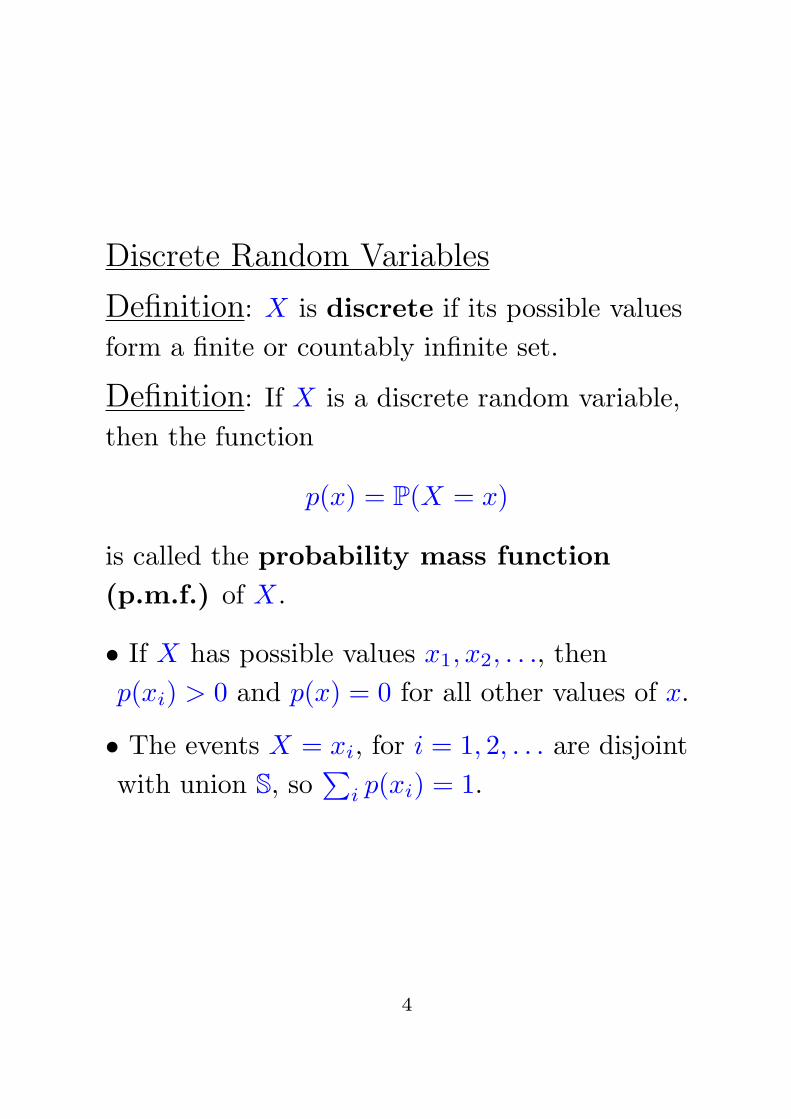
Definition: X is discrete if its possible valuesform a finite or countably infinite set.

Definition: If X is a discrete random variable,then the function

p(x) = P(X = x)

is called the probability mass function(p.m.f.) of X.

• If X has possible values x1, x2, . . ., thenp(xi) > 0 and p(x) = 0 for all other values of x.

• The events X = xi, for i = 1, 2, . . . are disjointwith union S, so

∑i p(xi) = 1.

4

Example. The probability mass function of arandom variable X is given by p(i) = c · λi/i!for i = 0, 1, 2, . . ., where λ is some positive value.Find

(i) P(X = 0)

(ii) P(X > 2)

5

Example. A baker makes 10 cakes on given day.Let X be the number sold. The baker estimatesthat X has p.m.f.

p(k) =120

+k

100, k = 0, 1, . . . , 10

Is this a plausible probability model?

Hint. Recall that∑n

i=1 i = 12n(n + 1). How do

you prove this?

6

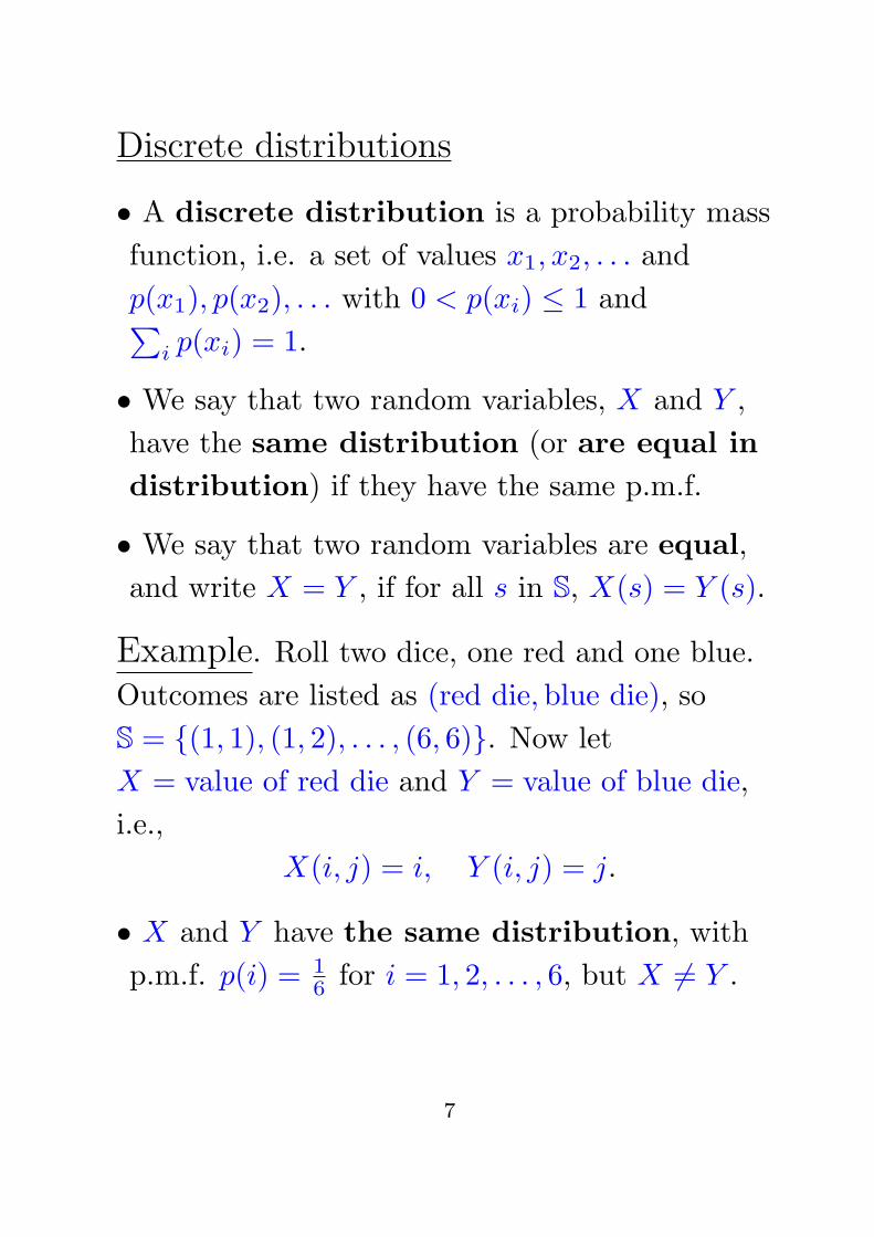
Discrete distributions

• A discrete distribution is a probability massfunction, i.e. a set of values x1, x2, . . . andp(x1), p(x2), . . . with 0 < p(xi) ≤ 1 and∑

i p(xi) = 1.

• We say that two random variables, X and Y ,have the same distribution (or are equal indistribution) if they have the same p.m.f.

• We say that two random variables are equal,and write X = Y , if for all s in S, X(s) = Y (s).

Example. Roll two dice, one red and one blue.Outcomes are listed as (red die,blue die), soS = {(1, 1), (1, 2), . . . , (6, 6)}. Now letX = value of red die and Y = value of blue die,i.e.,

X(i, j) = i, Y (i, j) = j.

• X and Y have the same distribution, withp.m.f. p(i) = 1

6 for i = 1, 2, . . . , 6, but X 6= Y .

7

The Cumulative Distribution Function

Definition: The c.d.f. of X is

F (x) = P(X ≤ x), for −∞ < x < ∞.

• We can also write FX(x) for the c.d.f. of X todistinguish it from the c.d.f. FY (y) of Y .

• Some related quantities are: (i) FX(x);(ii) FX(y); (iii) FX(X); (iv) Fx(Y ).

• Is (i) the same function as (ii)? Explain.

• Is (i) the same function as (iii)? Explain.

• What is the meaning, if any, of (iv)?

• Does it matter if we write the c.d.f of Y asFY (x) or FY (y)? Discuss.

8

• The c.d.f. contains the same information (for adiscrete distribution) as the p.m.f., since

F (x) =∑

xi≤x

p(xi)

p(xi) = F (xi)− F (xi − δ)

where δ is sufficiently small that none of thepossible values lies in the interval [xi − δ, xi).

• Sometimes it is more convenient to work withthe p.m.f. and sometimes with the c.d.f.

Example. Flip a fair coin until a head occurs.Let X be the length of the sequence. Find thep.m.f. of X, and plot it.

Solution.

9

Example Continued. Flip a fair coin until ahead occurs. Let X be the length of the sequence.Find the c.d.f. of X, and plot it.

Solution

Notation. It is useful to define bxc to be thelargest integer less than or equal to x.

10

Properties of the c.d.f.

Let X be a discrete RV with possible valuesx1, x2, . . . and c.d.f. F (x).

• 0 ≤ F (x) ≤ 1 . Why?

• F (x) is nondecreasing, i.e. if x ≤ y thenF (x) ≤ F (y). Why?

• limx→−∞ F (x) = 0 and limx→∞ F (x) = 1 .

Details are in Ross, Section 4.10.

11

Functions of a random variable

• Let X be a discrete RV with possible valuesx1, x2, . . . and p.m.f. pX(x).

• Let Y = g(X) for some function g mapping realnumbers to real numbers. Then Y is the randomvariable such that Y (s) = g

(X(s)

)for each

s ∈ S. Equivalently, Y is the random variablesuch that if X takes the value x, Y takes thevalue g(x).

Example. If X is the outcome of rolling a fairdie, and g(x) = x2, what is the p.m.f. ofY = g(X) = X2?

Solution.

12

Expectation

Consider the following game. A fair die is rolled,with the payoffs being...

Outcome Payoff ($) Probability

1 5 1/6

2,3,4 10 1/2

5,6 15 1/3

• How much would you pay to play this game?

• In the “long run”, if you played n times, thetotal payoff would be roughly

n

6× 5 +

n

2× 10 +

n

3× 15 = 10.83 n

• The average payoff per play is ≈ $ 10.83. This iscalled the expectation or expected value ofthe payoff. It is also called the fair price ofplaying the game.

13

Expectation of Discrete Random Variables

Definition. Let X be a discrete random variablewith possible values x1, x2, . . . and p.m.f. p(x).The expected value of X is

E(X) =∑

i xi p(xi)

• E(X) is a weighted average of the possiblevalues that X can take on.

• The expected value may not be a possible value.

Example. Flip a coin 3 times. Let X be thenumber of heads. Find E(X).

Solution.

14

Expectation of a Function of a RV

• If X is a discrete random variable, and g is afunction taking real numbers to real numbers,then g(X) is a discrete random variable also.

• If X has probability p(xi) of taking value xi,then g(X) does not necessarily take value g(xi)with probability p

(g(xi)

). Why? Nevertheless,

Proposition. E[g(X)

]=

∑i g(xi) p(xi)

Proof.

15

Example 1. Let X be the value of a fair die.

(i) Find E(X).

(ii) Find E(X2).

Example 2: Linearity of expectation.

For any random variable X and constants a and b,

E(aX + b) = a · E(X) + b

Proof.

16

Example. There are two questions in a quizshow. You get to choose the order to answerthem. If you try question 1 first, then you will beallowed to go on to question 2, only if youranswer to question 1 is correct, vice versa. Therewards for these two questions are V1 and V2. Ifthe probability that you know the answers to thetwo questions are p1 and p2, then which questionshould be chosen first?

17

Two intuitive properties of expectation

• The formula for expectation is the same as theformula for the center of mass, when objects ofmass pi are put at position xi. In other words,the expected value is the balancing point for thegraph of the probability mass function.

• The distribution of X is symmetric aboutsome point µ if p(µ + x) = p(µ− x) for every x.

If the distribution of X is symmetric about µ

then E(X) = µ. This is “obvious” from theintuition that the center of a symmetricdistribution should also be its balancing point.

18

Variance

• Expectation gives a measure of center of adistribution. Variance is a measure of spread.

Definition. If X is a random variable with meanµ, then the variance of X is

Var(X) = E[(X − µ)2

]

• The variance is the “expected squared deviationfrom average.”

• A useful identity is

Var(X) = E[X2

]− (E[X]

)2

Proof.

19

Proposition. For any RV X and constants a, b,

Var(aX + b) = a2 Var(X)

Proof.

Note 1. Intuitively, adding a constant, b, shouldchange the center of a distribution but not changeits spread.

Note 2. The a2 reminds us that variance isactually a measure of (spread)2. This isunintuitive.

20

Standard Deviation

• We might prefer to measure the spread of X inthe same units as X.

Definition. The standard deviation of X is

SD(X) =√

Var(X)

• A rule of thumb: Almost all the probabilitymass of a distribution lies within two standarddeviations of the mean.

Example. Let X be the value of a die. Find (i)E(X), (ii) Var(X), (iii) SD(X). Show the meanand standard deviation on a graph of the p.m.f.

Solution.

21

Example: standardization. Let X be arandom variable with expected value µ andstandard deviation σ. Find the expected value

and variance of Y =X − µ

σ.

Solution.

22

Bernoulli Random Variables

• The result of an experiment with two possibleoutcomes (e.g. flipping a coin) can be classifiedas either a success (with probability p) or afailure (with probability 1− p). Let X = 1 ifthe experiment is a success and X = 0 if it is afailure. Then the p.m.f. of X is p(1) = p,p(0) = 1− p.

• If the p.m.f. of a random variable can bewritten as above, it is said to be Bernoulli withparameter p.

• We write X ∼ Bernoulli(p).

23

Binomial Random Variables

Definition. Let X be the number of successes inn independent experiments each of which is asuccess (with probability p) and a failure (withprobability 1− p). X is said to be a binomialrandom variable with parameters (n, p). We writeX ∼ Binomial(n, p).

• If Xi is the Bernoulli random variablecorresponding to the ith trial, thenX =

∑ni=1 Xi.

• Whenever binomial random variables are usedas a chance model, look for the independenttrials with equal probability of success. Achance model is only as good as its assumptions!

24

The p.m.f. of the binomial distribution

• We write 1 for a success, 0 for a failure, so e.g.for n = 3, the sample space is

S = {000, 001, 010, 100, 011, 101, 110, 111}.• The probability of any particular sequence withk successes (so n− k failures) is

pk(1− p)n−k

• Therefore, if X ∼ Binomial(n, p), then

P(X = k) =(

n

k

)pk(1− p)(n−k)

for k = 0, 1, . . . , n.

• Where are independence and constant successprobability used in this calculation?

25

Example. A die is rolled 12 times. Find an

expression for the chance that 6 appears 3 ormore times.

Solution.

26

The Binomial Theorem. Suppose thatX ∼ Binomial(n, p). Since

∑nk=0 P(X = k) = 1,

we get the identity∑n

k=0

(nk

)pk(1− p)n−k = 1

Example. For the special case p = 1/2 we obtain

∑nk=0

(nk

)= 2n

This can also be calculated by counting subsets ofa set with n elements:

27

Expectation of the binomial distribution

Let X ∼ Binomial(n, p). What do you think theexpected value of X ought to be? Why?

Now check this by direct calculation...

28

Variance of the binomial distribution.

Let X ∼ Binomial(n, p). Show that

Var(X) = np(1− p)

Solution. We know(E[X]

)2 = n2p2. We have tofind E[X2].

29

Discussion problem. A system of n satellitesworks if at least k satellites are working. On acloudy day, each satellite works independentlywith probability p1 and on a clear day withprobability p2. If the chance of being cloudy is α,what is the chance that the system will beworking?

Solution

30

Binomial probabilities for large n, small p.

Let X ∼ Binomial(N, p/N). We look for a limitas N becomes large.

(1). Write out the binomial probability. Takelimits, recalling that the limit of a product is theproduct of the limits.

31

(2). Note that log[limN→∞

(1− p

N

)N]

=

limN→∞ log[(

1− pN

)N]. Why?

(3). Hence, show that limN→∞(1− p

N

)N = e−p.

(4). Using (3) and (1), obtain limN→∞ P(X = k).

32

The Poisson Distribution

• Binomial distributions with large n, small p

occur often in the natural world

Example: Nuclear decay. A large number ofunstable Uranium atoms decay independently,with some probability p in a fixed time interval.

Example: Prussian officers. In the 19thcentury Germany, each officer has some chance p

to be killed by a horse-kick each year.

Definition. A random variable X, taking on oneof the values 0, 1, 2, . . . is said to be a Poissonrandom variable with parameter λ > 0 if

p(k) = P(X = k) = e−λ λk

k!,

for k = 0, 1, . . ..

33

Example. The probability of a product beingdefective is 0.001. Compare the binomialdistribution with the Poisson approximation forfinding the probability that a sample of 1000items contain exactly 2 defective item.

Solution

34

Discussion problem. A cosmic ray detectorcounts, on average, ten events per day. Find thechance that no more than three are recorded on aparticular day.

Solution. It may be surprising that there isenough information in this question to provide areasonably unambiguous answer!

35

Expectation of the Poisson distribution

• Let X ∼ Poisson(λ), so P(X = k) = λke−k/k!.

Since X is approximately Binomial(N, λ/N), itwould not be surprising to find thatE[X] = N × λ

N = λ.

• We can show E[X] = λ by direct computation:

36

Variance of the Poisson distribution

• Let X ∼ Poisson(λ), so P(X = k) = λke−k/k!.

• The Binomial(N,λ/N) approximation suggestsVar(X) = limN →∞N × λ

N × (1− λ

N

)= λ.

• We can find E[X2] by direct computation tocheck this:

37

The Geometric Distribution

Definition. Independent trials (e.g. flipping acoin) until a success occurs. Let X be the numberof trials required. We write X ∼ Geometric(p).

• P(X = k) = p (1− p)k−1, for k = 1, 2, . . .

• E(X) = 1/p and Var(X) = (1− p)/p2

The Memoryless Property

Suppose X ∼ Geometric(p) and k, r > 0. Then

P(X > k + r|X > k) = P(X > r).

Why?

• This result shows that, conditional on nosuccesses before time k, X has forgotten the firstk failures, hence the Geometric distribution issaid to have a memoryless property.

38

Exercise. Let X ∼ Geometric(p). Derive theexpected value of X.

Solution.

39

Example 1. Suppose a fuse lasts for a number ofweeks X and X ∼ Geometric(1/52), so theexpected lifetime is E(X) = 52 weeks (≈ 1 year).Should I replace it if it is still working after twoyears?

Solution

Example 2. If I have rolled a die ten times andsee no 1, how long do I expect to wait (i.e. howmany more rolls do I have to make, on average)before getting a 1?

Solution

40

The Negative Binomial Distribution

Definition. For a sequence of independent trialswith chance p of success, let X be the number oftrials until r successes have occurred. Then X hasthe negative binomial distribution,X ∼ NegBin(p, r), with p.m.f.

P(X = k) =(k−1r−1

)pr(1− p)k−r

for k = r, r + 1, r + 2, . . .

• E(X) = r/p and Var(X) = r(1− p)/p2

• For r = 1, we can see that NegBin(p, 1) is thesame distribution as Geometric(p).

41

Example. One person in six is prepared toanswer a survey. Let X be the number of peopleasked in order to get 20 responses. What is themean and SD of X?

Solution.

42

The Hypergeometric Distribution

Definition. n balls are drawn randomly withoutreplacement from an urn containing N balls ofwhich m are white and N −m black. Let X bethe number of white balls drawn. Then X has thehypergeometric distribution,X ∼ Hypergeometric(m,n, N).

• P(X = k) =(mk

)(N−mn−k

)/(Nn

), for k = 0, 1, . . . ,m.

• E(X) = mnN = np and Var(X) = N−n

N−1 np(1− p),where p = m/N .

• Useful for analyzing sampling procedures.

• N here is not a random variable. We try to usecapital letters only for random variables, but thisconvention is sometimes violated.

43

Example: Capture-recapture experiments.

An unknown number of animals, say N , inhabit acertain region. To obtain some information aboutthe population size, ecologists catch a number,say m of them, mark them and release them.Later, n more are captured. Let X be the numberof marked animals in the second capture. What isthe most likely value of N?

Solution.

44