3. Aggregate Planning. Aggregate Planning Provides the quantity and timing of production for intermediate future Usually 3 to 18 months into future.

3. Aggregate Planning

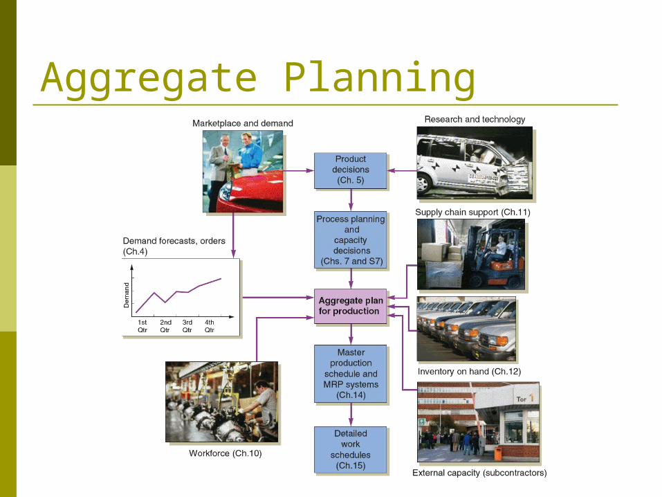
Aggregate Planning

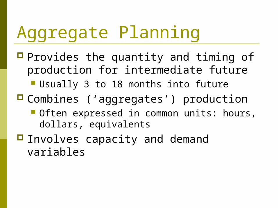
Aggregate Planning Provides the quantity and timing of

production for intermediate future Usually 3 to 18 months into future

Combines (‘aggregates’) production Often expressed in common units: hours,

dollars, equivalents Involves capacity and demand variables

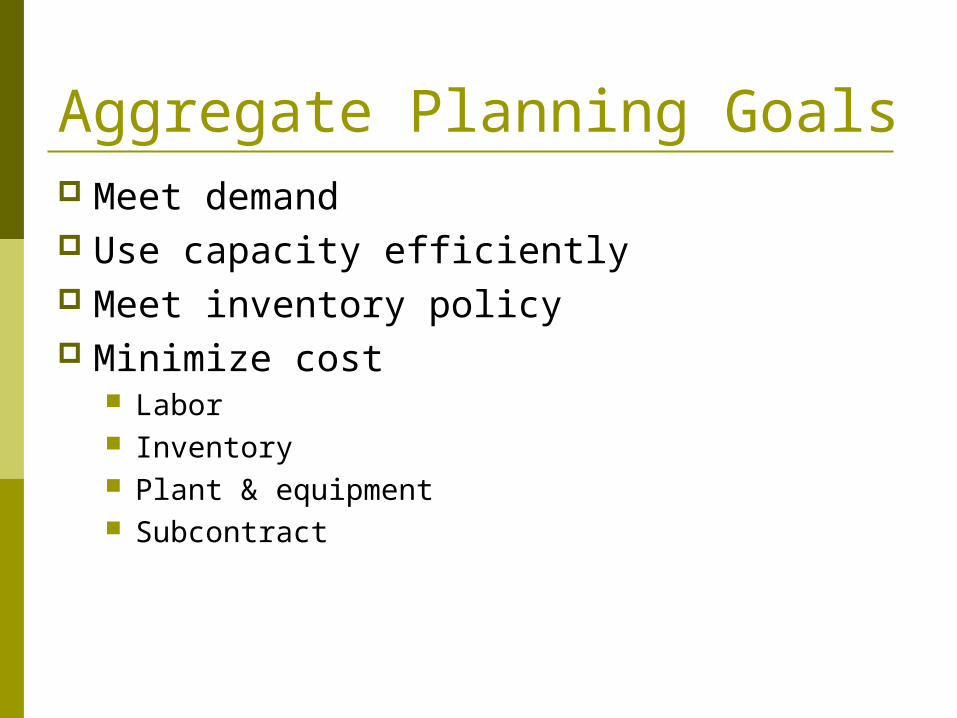
Aggregate Planning Goals Meet demand Use capacity efficiently Meet inventory policy Minimize cost

Labor Inventory Plant & equipment Subcontract

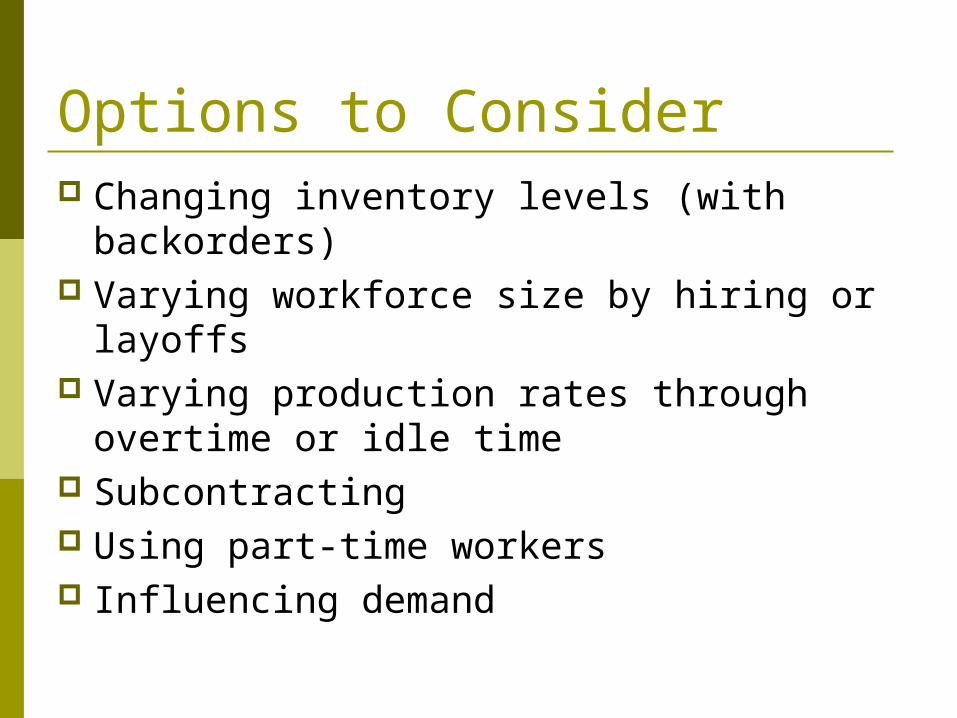
Options to Consider Changing inventory levels (with backorders) Varying workforce size by hiring or layoffs Varying production rates through overtime

or idle time Subcontracting Using part-time workers Influencing demand

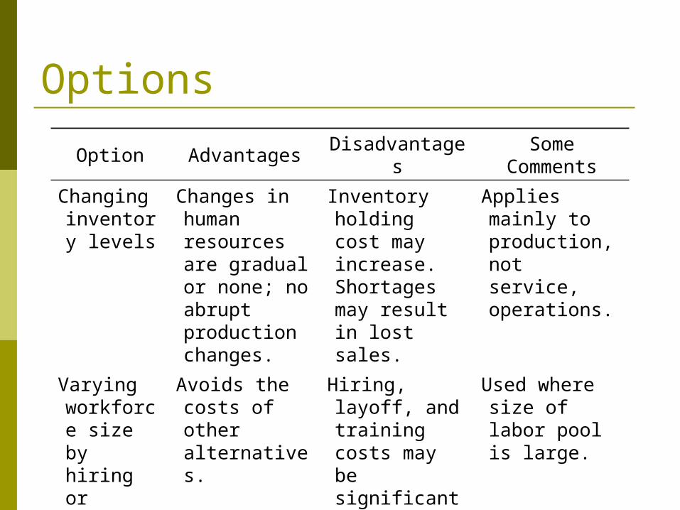
Option Advantages DisadvantagesSome

Comments

Changing inventory levels

Changes in human resources are gradual or none; no abrupt production changes.

Inventory holding cost may increase. Shortages may result in lost sales.

Applies mainly to production, not service, operations.

Varying workforce size by hiring or layoffs

Avoids the costs of other alternatives.

Hiring, layoff, and training costs may be significant.

Used where size of labor pool is large.

Options

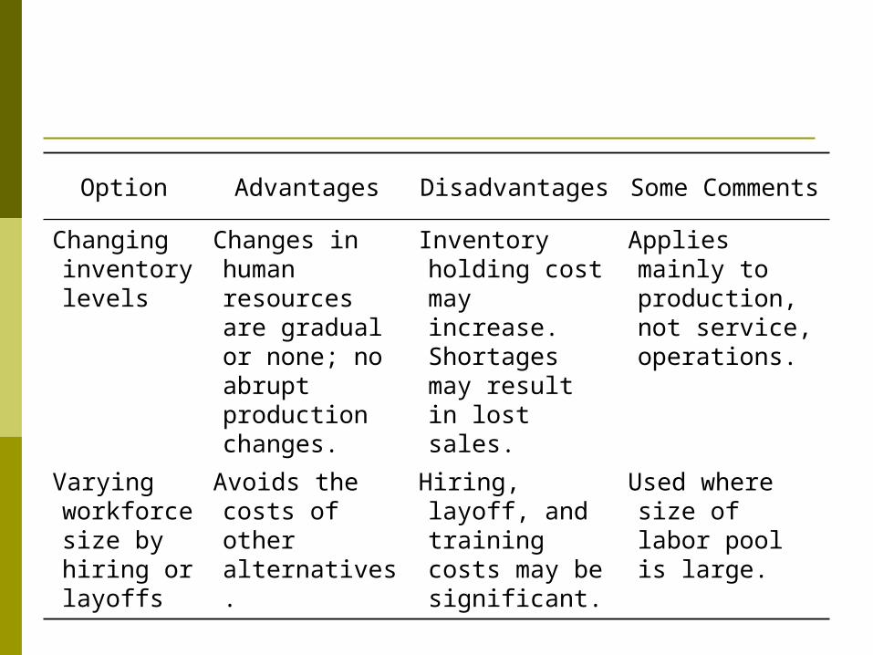
Option Advantages DisadvantagesSome

Comments

Changing inventory levels

Changes in human resources are gradual or none; no abrupt production changes.

Inventory holding cost may increase. Shortages may result in lost sales.

Applies mainly to production, not service, operations.

Varying workforce size by hiring or layoffs

Avoids the costs of other alternatives.

Hiring, layoff, and training costs may be significant.

Used where size of labor pool is large.

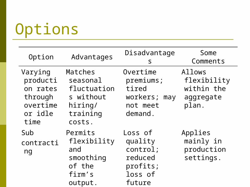
Option Advantages DisadvantagesSome

Comments

Varying production rates through overtime or idle time

Matches seasonal fluctuations without hiring/ training costs.

Overtime premiums; tired workers; may not meet demand.

Allows flexibility within the aggregate plan.

Subcontracting

Permits flexibility and smoothing of the firm’s output.

Loss of quality control; reduced profits; loss of future business.

Applies mainly in production settings.

Options

Option Advantages DisadvantagesSome

Comments

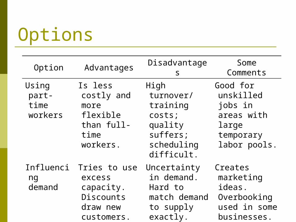
Using part-time workers

Is less costly and more flexible than full-time workers.

High turnover/ training costs; quality suffers; scheduling difficult.

Good for unskilled jobs in areas with large temporary labor pools.

Influencing demand

Tries to use excess capacity. Discounts draw new customers.

Uncertainty in demand. Hard to match demand to supply exactly.

Creates marketing ideas. Overbooking used in some businesses.

Options

Option Advantages DisadvantagesSome

Comments

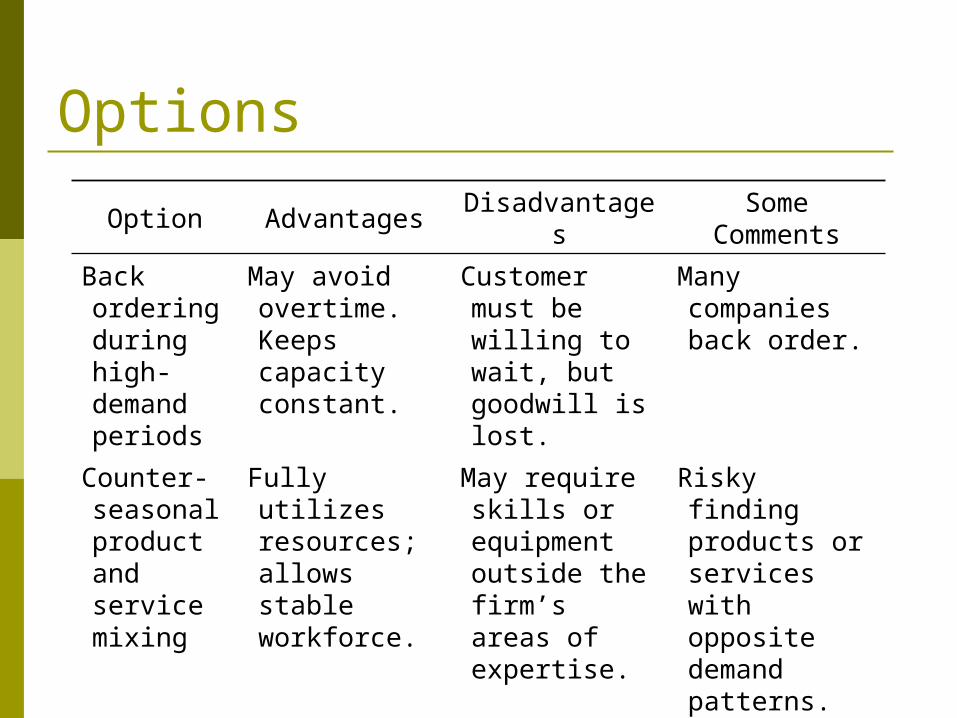
Back ordering during high-demand periods

May avoid overtime. Keeps capacity constant.

Customer must be willing to wait, but goodwill is lost.

Many companies back order.

Counter-seasonal product and service mixing

Fully utilizes resources; allows stable workforce.

May require skills or equipment outside the firm’s areas of expertise.

Risky finding products or services with opposite demand patterns.

Options

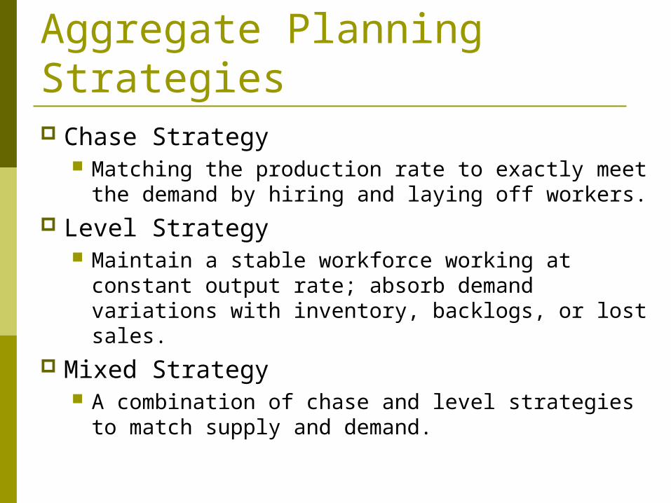
Aggregate Planning Strategies Chase Strategy

Matching the production rate to exactly meet the demand by hiring and laying off workers.

Level Strategy Maintain a stable workforce working at constant

output rate; absorb demand variations with inventory, backlogs, or lost sales.

Mixed Strategy A combination of chase and level strategies to

match supply and demand.

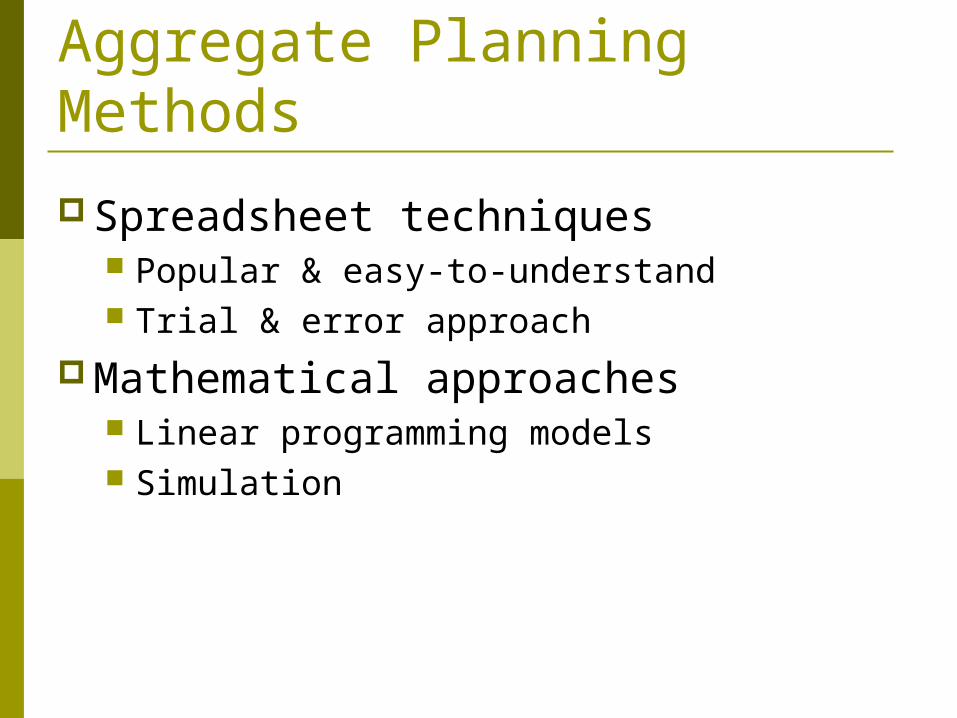
Aggregate Planning Methods

Spreadsheet techniques Popular & easy-to-understand Trial & error approach

Mathematical approaches Linear programming models Simulation

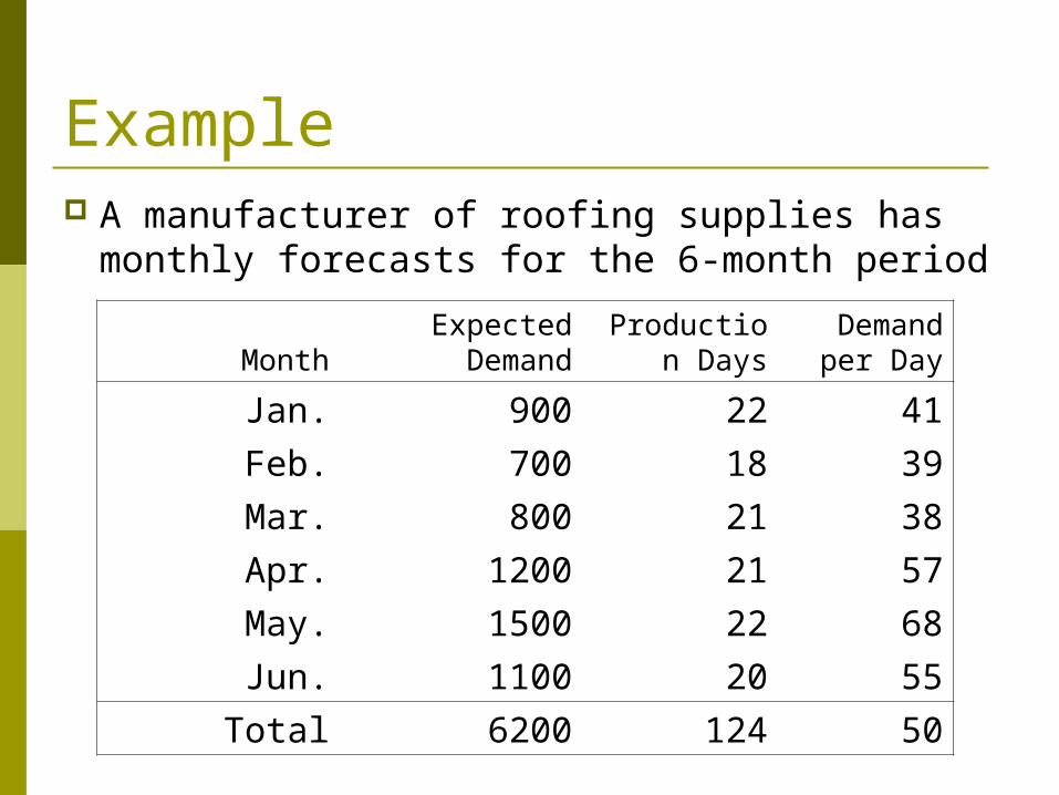
Example A manufacturer of roofing supplies has

monthly forecasts for the 6-month period

MonthExpected Demand

Production Days

Demand per Day

Jan. 900 22 41

Feb. 700 18 39

Mar. 800 21 38

Apr. 1200 21 57

May. 1500 22 68

Jun. 1100 20 55

Total 6200 124 50

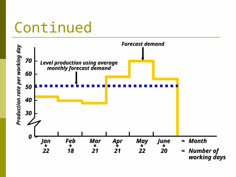
Continued

70 70 –

60 60 –

50 50 –

40 40 –

30 30 –

0 0 –JanJan FebFeb MarMar AprApr MayMay JuneJune == MonthMonth

2222 1818 2121 2121 2222 2020 == Number ofNumber ofworking daysworking days

Pro

du

ctio

n r

ate

per

wo

rkin

g d

ayP

rod

uct

ion

rat

e p

er w

ork

ing

day

Level production using average Level production using average monthly forecast demandmonthly forecast demand

Forecast demandForecast demand

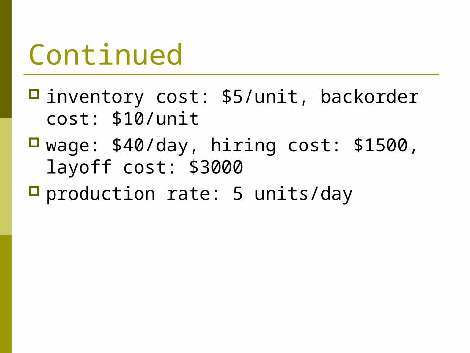
Continued inventory cost: $5/unit, backorder cost:

$10/unit wage: $40/day, hiring cost: $1500, layoff

cost: $3000 production rate: 5 units/day

Chase Strategy  Jan. Feb. Mar. Apr. May. Jun. Total

Forecast 900 700 800 1200 1500 1100 6200

Working days 22 18 21 21 22 20 124

Demand per day 40.9 38.9 38.1 57.1 68.2 55.0 50.0

Workers available 8  

Hired/Fired  

H/F cost  

Labor cost  

Units Produced  

Net inventory  

Inventory cost  

Total cost              

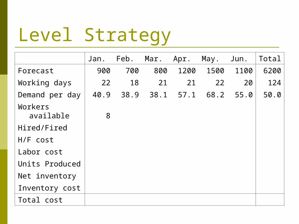
Level Strategy  Jan. Feb. Mar. Apr. May. Jun. Total

Forecast 900 700 800 1200 1500 1100 6200

Working days 22 18 21 21 22 20 124

Demand per day 40.9 38.9 38.1 57.1 68.2 55.0 50.0

Workers available 8  

Hired/Fired  

H/F cost  

Labor cost  

Units Produced  

Net inventory  

Inventory cost  

Total cost              

Mixed Strategy  Jan. Feb. Mar. Apr. May. Jun. Total

Forecast 900 700 800 1200 1500 1100 6200

Working days 22 18 21 21 22 20 124

Demand per day 40.9 38.9 38.1 57.1 68.2 55.0 50.0

Workers available 8  

Hired/Fired  

H/F cost  

Labor cost  

Units Produced  

Net inventory  

Inventory cost  

Total cost              

Linear Programming Models Workforce planning model Production planning model

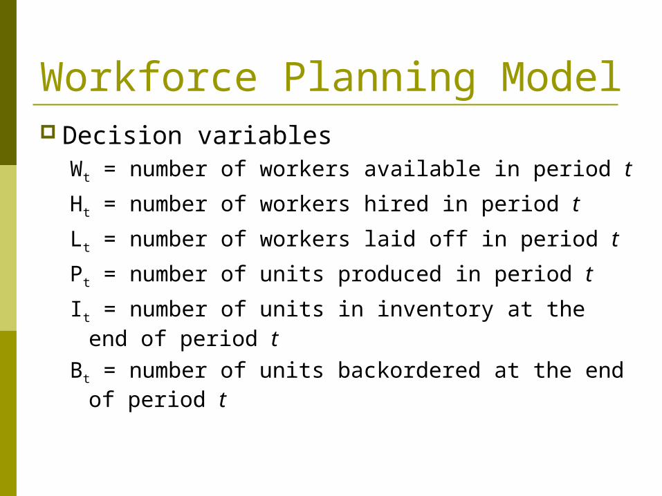
Workforce Planning Model Decision variables

Wt = number of workers available in period t

Ht = number of workers hired in period t

Lt = number of workers laid off in period t

Pt = number of units produced in period t

It = number of units in inventory at the end of period t

Bt = number of units backordered at the end of period t

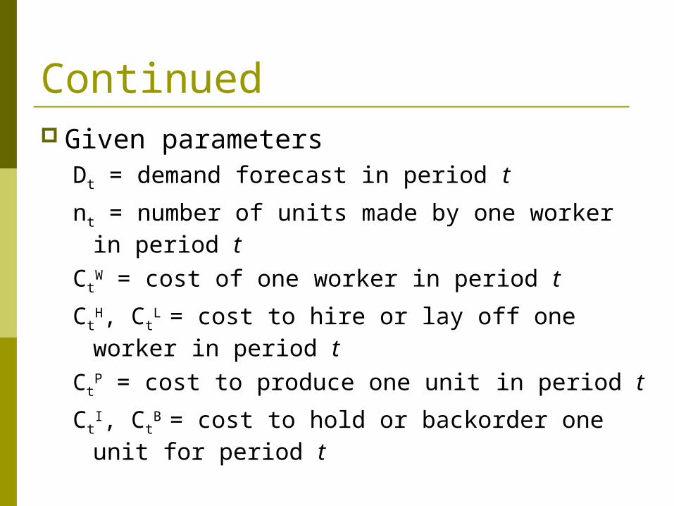
Continued Given parameters

Dt = demand forecast in period t

nt = number of units made by one worker in period t

CtW = cost of one worker in period t

CtH, Ct

L = cost to hire or lay off one worker in period t

CtP = cost to produce one unit in period t

CtI, Ct

B = cost to hold or backorder one unit for period t

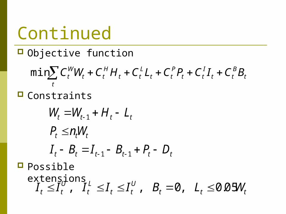
Continued Objective function

Constraints

Possible extensions

t

tBtt

Itt

Ptt

Ltt

Htt

Wt BCICPCLCHCWCmin

tttttt

ttt

tttt

DPBIBI

WnP

LHWW

11

1

tttUtt

Lt

Utt WLBIIIII 05.0,0,,

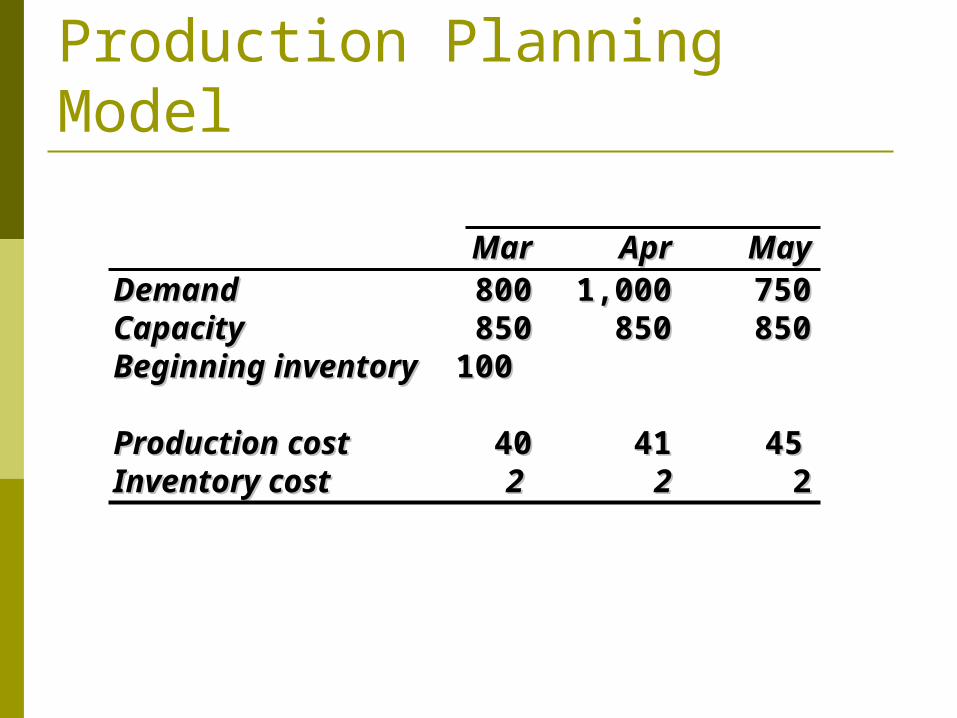
Production Planning Model

MarMar AprApr MayMay

DemandDemand 800800 1,0001,000 750750CapacityCapacity 850850 850850 850850Beginning inventoryBeginning inventory 100100

Production costProduction cost 4040 4141 4545 Inventory costInventory cost 2 2 22 22

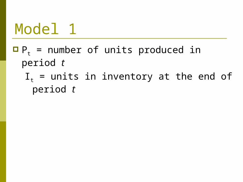
Model 1 Pt = number of units produced in period t

It = units in inventory at the end of period t

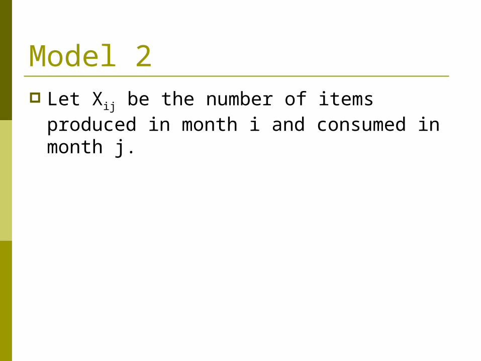
Model 2 Let Xij be the number of items produced in

month i and consumed in month j.

Another Example

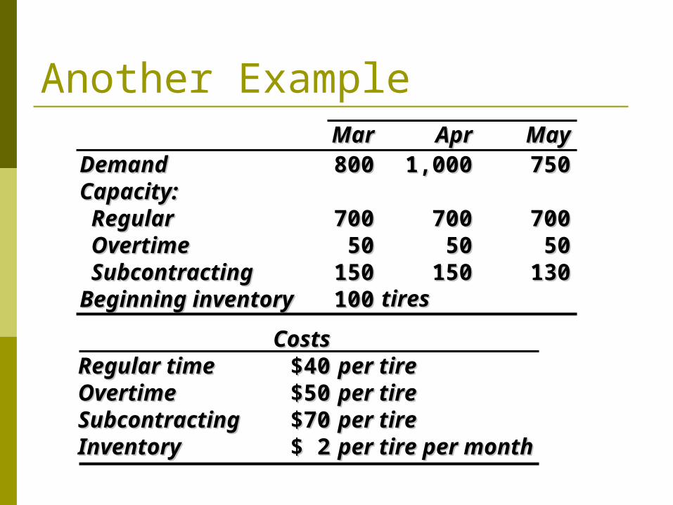
CostsCostsRegular timeRegular time $40$40 per tireper tireOvertimeOvertime $50$50 per tireper tireSubcontractingSubcontracting $70$70 per tireper tireInventoryInventory $ 2$ 2 per tire per monthper tire per month

MarMar AprApr MayMay

DemandDemand 800800 1,0001,000 750750Capacity:Capacity: RegularRegular 700700 700700 700700 OvertimeOvertime 5050 5050 5050 SubcontractingSubcontracting 150150 150150 130130Beginning inventoryBeginning inventory 100100 tirestires

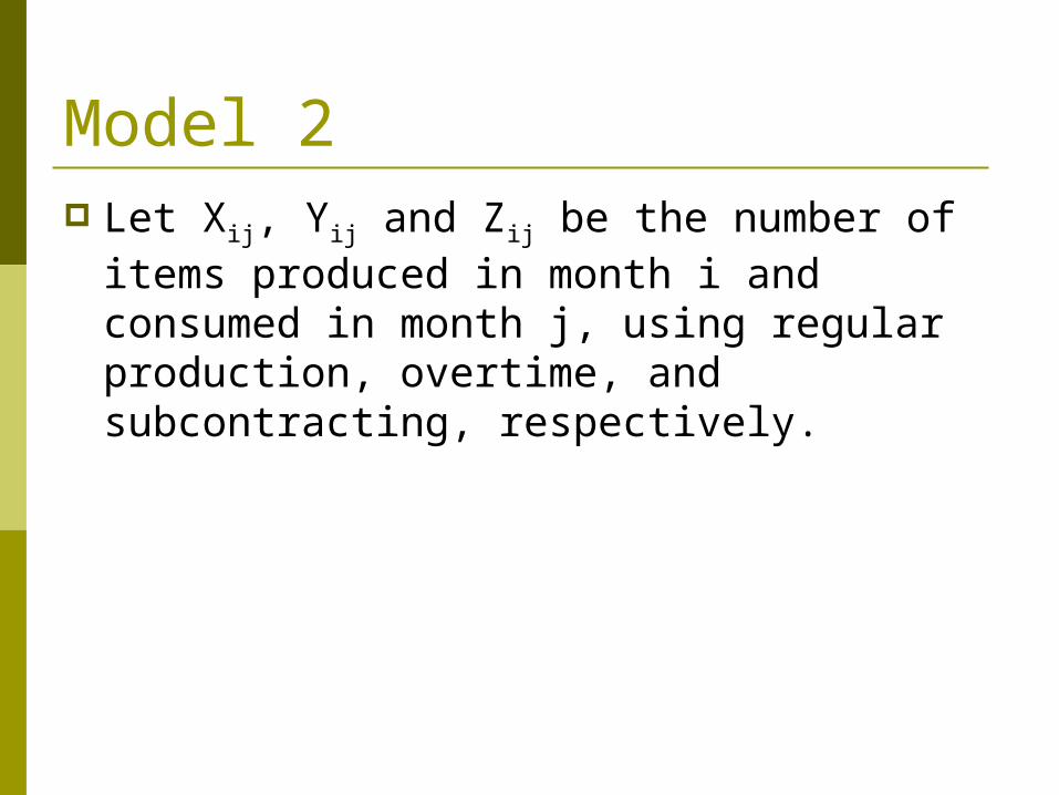
Model 2 Let Xij, Yij and Zij be the number of items

produced in month i and consumed in month j, using regular production, overtime, and subcontracting, respectively.