2. The Quantum String - University of Cambridge · 2. The Quantum String ... • The alternative method is to first solve all of the constraints of the system to ... towers of creation

2. The Quantum String

Our goal in this section is to quantize the string. We have seen that the string action

involves a gauge symmetry and whenever we wish to quantize a gauge theory we’re

presented with a number of di↵erent ways in which we can proceed. If we’re working

in the canonical formalism, this usually boils down to one of two choices:

• We could first quantize the system and then subsequently impose the constraints

that arise from gauge fixing as operator equations on the physical states of the

system. For example, in QED this is the Gupta-Bleuler method of quantization

that we use in Lorentz gauge. In string theory it consists of treating all fields Xµ,

including time X0, as operators and imposing the constraint equations (1.33) on

the states. This is usually called covariant quantization.

• The alternative method is to first solve all of the constraints of the system to

determine the space of physically distinct classical solutions. We then quantize

these physical solutions. For example, in QED, this is the way we proceed in

Coulomb gauge. Later in this chapter, we will see a simple way to solve the

constraints of the free string.

Of course, if we do everything correctly, the two methods should agree. Usually, each

presents a slightly di↵erent challenge and o↵ers a di↵erent viewpoint.

In these lectures, we’ll take a brief look at the first method of covariant quantization.

However, at the slightest sign of di�culties, we’ll bail! It will be useful enough to

see where the problems lie. We’ll then push forward with the second method described

above which is known as lightcone quantization in string theory. Although we’ll succeed

in pushing quantization through to the end, our derivations will be a little cheap and

unsatisfactory in places. In Section 5 we’ll return to all these issues, armed with more

sophisticated techniques from conformal field theory.

2.1 A Lightning Look at Covariant Quantization

We wish to quantize D free scalar fields Xµ whose dynamics is governed by the action

(1.30). We subsequently wish to impose the constraints

X ·X 0 = X2 +X 0 2 = 0 . (2.1)

The first step is easy. We promote Xµ and their conjugate momenta ⇧µ = (1/2⇡↵0)Xµ

to operator valued fields obeying the canonical equal-time commutation relations,

[Xµ(�, ⌧),⇧⌫(�0, ⌧)] = i�(� � �0) �µ⌫ ,

[Xµ(�, ⌧), X⌫(�0, ⌧)] = [⇧µ(�, ⌧),⇧⌫(�0, ⌧)] = 0 .

– 28 –

We translate these into commutation relations for the Fourier modes xµ, pµ, ↵µn and

↵µn. Using the mode expansion (1.36) we find

[xµ, p⌫ ] = i�µ⌫ and [↵µn,↵

⌫m] = [↵µ

n, ↵⌫m] = n ⌘µ⌫�n+m, 0 , (2.2)

with all others zero. The commutation relations for xµ and pµ are expected for oper-

ators governing the position and momentum of the center of mass of the string. The

commutation relations of ↵µn and ↵µ

n are those of harmonic oscillator creation and anni-

hilation operators in disguise. And the disguise isn’t that good. We just need to define

(ignoring the µ index for now)

an =↵npn

, a†n =↵�npn

n > 0 (2.3)

Then (2.2) gives the familiar [an, a†m] = �mn. So each scalar field gives rise to two infinite

towers of creation and annihilation operators, with ↵n acting as a rescaled annihilation

operator for n > 0 and as a creation operator for n < 0. There are two towers because

we have right-moving modes ↵n and left-moving modes ↵n.

With these commutation relations in hand we can now start building the Fock space

of our theory. We introduce a vacuum state of the string |0i, defined to obey

↵µn |0i = ↵µ

n |0i = 0 for n > 0 (2.4)

The vacuum state of string theory has a di↵erent interpretation from the analogous

object in field theory. This is not the vacuum state of spacetime. It is instead the

vacuum state of a single string. This is reflected in the fact that the operators xµ

and pµ give extra structure to the vacuum. The true ground state of the string is |0i,tensored with a spatial wavefunction (x). Alternatively, if we work in momentum

space, the vacuum carries another quantum number, pµ, which is the eigenvalue of the

momentum operator. We should therefore write the vacuum as |0; pi, which still obeys

(2.4), but now also

pµ |0; pi = pµ|0; pi (2.5)

where (for the only time in these lecture notes) we’ve put a hat on the momentum

operator pµ on the left-hand side of this equation to distinguish it from the eigenvalue

pµ on the right-hand side.

We can now start to build up the Fock space by acting with creation operators ↵µn

and ↵µn with n < 0. A generic state comes from acting with any number of these

creation operators on the vacuum,

(↵µ1�1

)nµ1 (↵µ2�2

)nµ2 . . . (↵⌫1�1

)n⌫1 (↵⌫2�2

)n⌫2 . . . |0; pi

– 29 –

Each state in the Fock space is a di↵erent excited state of the string. Each has the

interpretation of a di↵erent species of particle in spacetime. We’ll see exactly what

particles they are shortly. But for now, notice that because there’s an infinite number

of ways to excite a string there are an infinite number of di↵erent species of particles

in this theory.

2.1.1 Ghosts

There’s a problem with the Fock space that we’ve constructed: it doesn’t have positive

norm. The reason for this is that one of the scalar fields, X0, comes with the wrong sign

kinetic term in the action (1.30). From the perspective of the commutation relations,

this issue raises its head in presence of the spacetime Minkowski metric in the expression

[↵µn,↵

⌫ †m ] = n ⌘µ⌫ �n,m .

This gives rise to the o↵ending negative norm states, which come with an odd number

of timelike oscillators excited, for example

hp0; 0|↵0

1

↵0

�1

|0; pi ⇠ ��D(p� p0)

This is the first problem that arises in the covariant approach to quantization. States

with negative norm are referred to as ghosts. To make sense of the theory, we have

to make sure that they can’t be produced in any physical processes. Of course, this

problem is familiar from attempts to quantize QED in Lorentz gauge. In that case,

gauge symmetry rides to the rescue since the ghosts are removed by imposing the gauge

fixing constraint. We must hope that the same happens in string theory.

2.1.2 Constraints

Although we won’t push through with this programme at the present time, let us briefly

look at what kind of constraints we have in string theory. In terms of Fourier modes,

the classical constraints can be written as Ln = Ln = 0, where

Ln =1

2

Xm

↵n�m · ↵m

and similar for Ln. As in the Gupta-Bleuler quantization of QED, we don’t impose all

of these as operator equations on the Hilbert space. Instead we only require that the

operators Ln and Ln have vanishing matrix elements when sandwiched between two

physical states |physi and |phys0i,

hphys0|Ln|physi = hphys0|Ln|physi = 0

– 30 –

Because L†n = L�n, it is therefore su�cient to require

Ln|physi = Ln|physi = 0 for n > 0 (2.6)

However, we still haven’t explained how to impose the constraints L0

and L0

. And

these present a problem that doesn’t arise in the case of QED. The problem is that,

unlike for Ln with n 6= 0, the operator L0

is not uniquely defined when we pass to the

quantum theory. There is an operator ordering ambiguity arising from the commuta-

tion relations (2.2). Commuting the ↵µn operators past each other in L

0

gives rise to

extra constant terms.

Question: How do we know what order to put the ↵µn operators in the quantum

operator L0

? Or the ↵µn operators in L

0

?

Answer: We don’t! Yet. Naively it looks as if each di↵erent choice will define a

di↵erent theory when we impose the constraints. To make this ambiguity manifest, for

now let’s just pick a choice of ordering. We define the quantum operators to be normal

ordered, with the annihilation operators ↵in, n > 0, moved to the right,

L0

=1X

m=1

↵�m · ↵m +1

2↵2

0

, L0

=1X

m=1

↵�m · ↵m +1

2↵2

0

Then the ambiguity rears its head in the di↵erent constraint equations that we could

impose, namely

(L0

� a)|physi = (L0

� a)|physi = 0 (2.7)

for some constant a.

As we saw classically, the operators L0

and L0

play an important role in determining

the spectrum of the string because they include a term quadratic in the momentum

↵µ0

= ↵µ0

=p↵0/2 pµ. Combining the expression (1.41) with our constraint equation

for L0

and L0

, we find the spectrum of the string is given by,

M2 =4

↵0

�a+

1Xm=1

↵�m · ↵m

!=

4

↵0

�a+

1Xm=1

↵�m · ↵m

!We learn therefore that the undetermined constant a has a direct physical e↵ect: it

changes the mass spectrum of the string. In the quantum theory, the sums over ↵µn

modes are related to the number operators for the harmonic oscillator: they count the

number of excited modes of the string. The level matching in the quantum theory

tells us that the number of left-moving modes must equal the number of right-moving

modes.

– 31 –

Ultimately, we will find that the need to decouple the ghosts forces us to make a

unique choice for the constant a. (Spoiler alert: it turns out to be a = 1). In fact, the

requirement that there are no ghosts is much stronger than this. It also restricts the

number of scalar fields that we have in the theory. (Another spoiler: D = 26). If you’re

interested in how this works in covariant formulation then you can read about it in the

book by Green, Schwarz and Witten. Instead, we’ll show how to quantize the string

and derive these values for a and D in lightcone gauge. However, after a trip through

the world of conformal field theory, we’ll come back to these ideas in a context which

is closer to the covariant approach.

2.2 Lightcone Quantization

We will now take the second path described at the beginning of this section. We will

try to find a parameterization of all classical solutions of the string. This is equivalent

to finding the classical phase space of the theory. We do this by solving the constraints

(2.1) in the classical theory, leaving behind only the physical degrees of freedom.

Recall that we fixed the gauge to set the worldsheet metric to

g↵� = ⌘↵� .

However, this isn’t the end of our gauge freedom. There still remain gauge transforma-

tions which preserve this choice of metric. In particular, any coordinate transformation

� ! �(�) which changes the metric by

⌘↵� ! ⌦2(�)⌘↵� , (2.8)

can be undone by a Weyl transformation. What are these coordinate transformations?

It’s simplest to answer this using lightcone coordinates on the worldsheet,

�± = ⌧ ± � , (2.9)

where the flat metric on the worldsheet takes the form,

ds2 = �d�+d��

In these coordinates, it’s clear that any transformation of the form

�+ ! �+(�+) , �� ! ��(��) , (2.10)

simply multiplies the flat metric by an overall factor (2.8) and so can be undone by

a compensating Weyl transformation. Some quick comments on this surviving gauge

symmetry:

– 32 –

• Recall that in Section 1.3.2 we used the argument that 3 gauge invariances (2

reparameterizations + 1 Weyl) could be used to fix 3 components of the world-

sheet metric g↵�. What happened to this argument? Why do we still have some

gauge symmetry left? The reason is that �± are functions of just a single variable,

not two. So we did fix nearly all our gauge symmetries. What is left is a set of

measure zero amongst the full gauge symmetry that we started with.

• The remaining reparameterization invariance (2.10) has an important physical

implication. Recall that the solutions to the equations of motion are of the form

XµL(�

+) + XµR(�

�) which looks like 2D functions worth of solutions. Of course,

we still have the constraints which, in terms of �±, read

(@+

X)2 = (@�X)2 = 0 , (2.11)

which seems to bring the number down to 2(D� 1) functions. But the reparam-

eterization invariance (2.10) tells us that even some of these are fake since we

can always change what we mean by �±. The physical solutions of the string are

therefore actually described by 2(D � 2) functions. But this counting has a nice

interpretation: the degrees of freedom describe the transverse fluctuations of the

string.

• The above comment reaches the same conclusion as the discussion in Section

1.3.2. There, in an attempt to get some feel for the constraints, we claimed that

we could go to static gauge X0 = R⌧ for some dimensionful parameter R. It

is easy to check that this is simple to do using reparameterizations of the form

(2.10). However, to solve the string constraints in full, it turns out that static

gauge is not that useful. Rather we will use something called “lightcone gauge”.

2.2.1 Lightcone Gauge

We would like to gauge fix the remaining reparameterization invariance (2.10). The best

way to do this is called lightcone gauge. In counterpoint to the worldsheet lightcone

coordinates (2.9), we introduce the spacetime lightcone coordinates,

X± =

r1

2(X0 ±XD�1) . (2.12)

Note that this choice picks out a particular time direction and a particular spatial

direction. It means that any calculations that we do involvingX± will not be manifestly

Lorentz invariant. You might think that we needn’t really worry about this. We could

try to make the following argument: “The equations may not look Lorentz invariant

– 33 –

but, since we started from a Lorentz invariant theory, at the end of the day any physical

process is guaranteed to obey this symmetry”. Right?! Well, unfortunately not. One

of the more interesting and subtle aspects of quantum field theory is the possibility of

anomalies: these are symmetries of the classical theory that do not survive the journey

of quantization. When we come to the quantum theory, if our equations don’t look

Lorentz invariant then there’s a real possibility that it’s because the underlying physics

actually isn’t Lorentz invariant. Later we will need to spend some time figuring out

under what circumstances our quantum theory keeps the classical Lorentz symmetry.

In lightcone coordinates, the spacetime Minkowski metric reads

ds2 = �2dX+dX� +D�2Xi=1

dX idX i

This means that indices are raised and lowered with A+

= �A� and A� = �A+ and

Ai = Ai. The product of spacetime vectors reads A · B = �A+B� � A�B+ + AiBi.

Let’s look at the solution to the equation of motion for X+. It reads,

X+ = X+

L (�+) +X+

R (��) .

We now gauge fix. We use our freedom of reparameterization invariance to choose

coordinates such that

X+

L = 1

2

x+ + 1

2

↵0p+�+ , X+

R = 1

2

x+ + 1

2

↵0p+�� .

You might think that we could go further and eliminate p+X

+

Figure 9:

and x+ but this isn’t possible because we don’t quite have

the full freedom of reparameterization invariance since all

functions should remain periodic in �. The upshot of this

choice of gauge is that

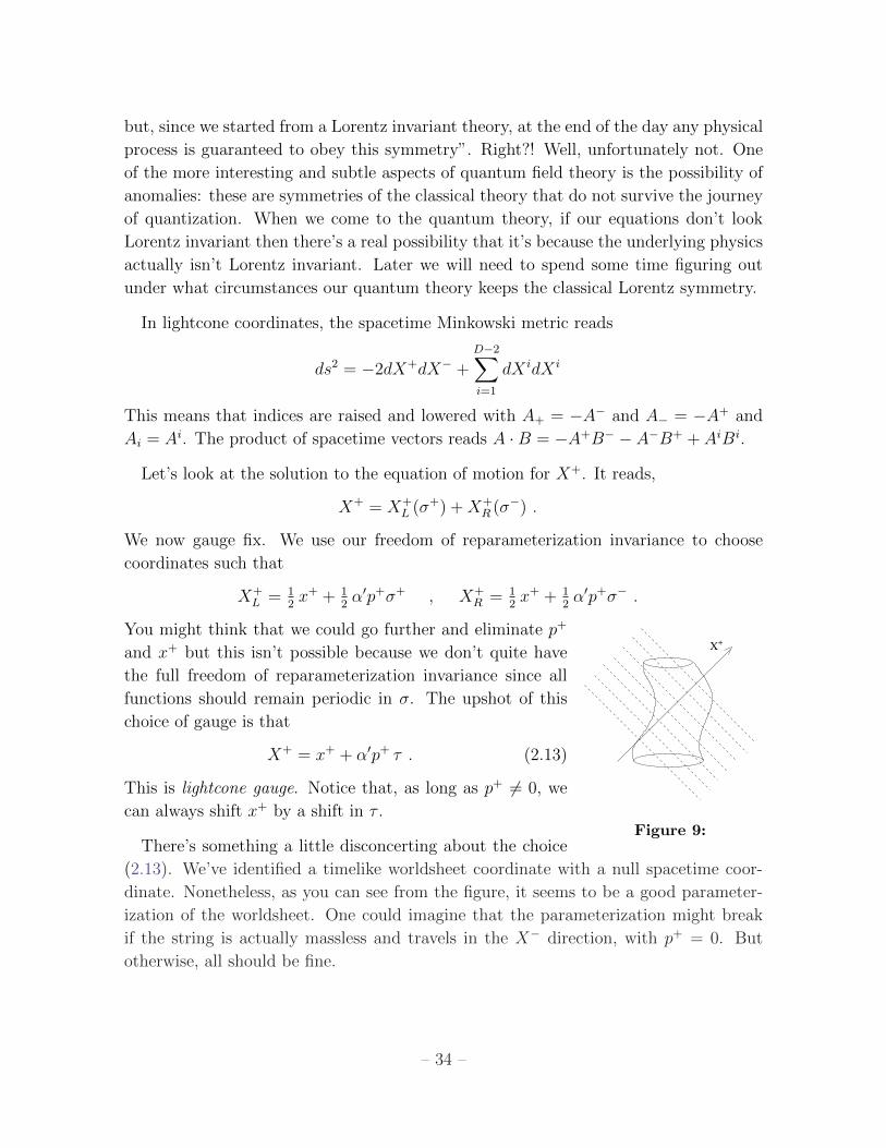
X+ = x+ + ↵0p+ ⌧ . (2.13)

This is lightcone gauge. Notice that, as long as p+ 6= 0, we

can always shift x+ by a shift in ⌧ .

There’s something a little disconcerting about the choice

(2.13). We’ve identified a timelike worldsheet coordinate with a null spacetime coor-

dinate. Nonetheless, as you can see from the figure, it seems to be a good parameter-

ization of the worldsheet. One could imagine that the parameterization might break

if the string is actually massless and travels in the X� direction, with p+ = 0. But

otherwise, all should be fine.

– 34 –

Solving for X�

The choice (2.13) does the job of fixing the reparameterization invariance (2.10). As

we will now see, it also renders the constraint equations trivial. The first thing that we

have to worry about is the possibility of extra constraints arising from this new choice

of gauge fixing. This can be checked by looking at the equation of motion for X+,

@+

@�X� = 0

But we can solve this by the usual ansatz,

X� = X�L (�

+) +X�R (�

�) .

We’re still left with all the other constraints (2.11). Here we see the real benefit of

working in lightcone gauge (which is actually what makes quantization possible at all):

X� is completely determined by these constraints. For example, the first of these reads

2@+

X�@+

X+ =D�2Xi=1

@+

X i@+

X i (2.14)

which, using (2.13), simply becomes

@+

X�L =

1

↵0p+

D�2Xi=1

@+

X i@+

X i . (2.15)

Similarly,

@�X�R =

1

↵0p+

D�2Xi=1

@�Xi@�X

i . (2.16)

So, up to an integration constant, the function X�(�+, ��) is completely determined

in terms of the other fields. If we write the usual mode expansion for X�L/R

X�L (�

+) = 1

2

x� + 1

2

↵0p� �+ + i

r↵0

2

Xn 6=0

1

n↵�n e�in�+

,

X�R (�

�) = 1

2

x� + 1

2

↵0p� �� + i

r↵0

2

Xn 6=0

1

n↵�n e�in��

.

then x� is the undetermined integration constant, while p�, ↵�n and ↵�

n are all fixed by

the constraints (2.15) and (2.16). For example, the oscillator modes ↵�n are given by,

↵�n =

r1

2↵01

p+

+1Xm=�1

D�2Xi=1

↵in�m↵

im , (2.17)

– 35 –

A special case of this is the ↵�0

=p↵0/2 p� equation, which reads

↵0p�

2=

1

2p+

D�2Xi=1

1

2

↵0pipi +Xn 6=0

↵in↵

i�n

!. (2.18)

We also get another equation for p� from the ↵�0

equation arising from (2.15)

↵0p�

2=

1

2p+

D�2Xi=1

1

2

↵0pipi +Xn 6=0

↵in↵

i�n

!. (2.19)

From these two equations, we can reconstruct the old, classical, level matching condi-

tions (1.41). But now with a di↵erence:

M2 = 2p+p� �D�2Xi=1

pipi =4

↵0

D�2Xi=1

Xn>0

↵i�n↵

in =

4

↵0

D�2Xi=1

Xn>0

↵i�n↵

in . (2.20)

The di↵erence is that now the sum is over oscillators ↵i and ↵i only, with i = 1, . . . , D�2. We’ll refer to these as transverse oscillators. Note that the string isn’t necessarily

living in the X0-XD�1 plane, so these aren’t literally the transverse excitations of the

string. Nonetheless, if we specify the ↵i then all other oscillator modes are determined.

In this sense, they are the physical excitation of the string.

Let’s summarize the state of play so far. The most general classical solution is

described in terms of 2(D � 2) transverse oscillator modes ↵in and ↵i

n, together with

a number of zero modes describing the center of mass and momentum of the string:

xi, pi, p+ and x�. But x+ can be absorbed by a shift of ⌧ in (2.13) and p� is constrained

to obey (2.18) and (2.19). In fact, p� can be thought of as (proportional to) the

lightcone Hamiltonian. Indeed, we know that p� generates translations in x+, but this

is equivalent to shifts in ⌧ .

2.2.2 Quantization

Having identified the physical degrees of freedom, let’s now quantize. We want to

impose commutation relations. Some of these are easy:

[xi, pj] = i�ij , [x�, p+] = �i

[↵in,↵

jm] = [↵i

n, ↵jm] = n�ij�n+m,0 . (2.21)

– 36 –

all of which follow from the commutation relations (2.2) that we saw in covariant

quantization1.

What to do with x+ and p�? We could implement p� as the Hamiltonian acting on

states. In fact, it will prove slightly more elegant (but equivalent) if we promote both

x+ and p� to operators with the expected commutation relation,

[x+, p�] = �i . (2.22)

This is morally equivalent to writing [t,H] = �i in non-relativistic quantum mechanics,

which is true on a formal level. In the present context, it means that we can once again

choose states to be eigenstates of pµ, with µ = 0, . . . , D, but the constraints (2.18) and

(2.19) must still be imposed as operator equations on the physical states. We’ll come

to this shortly.

The Hilbert space of states is very similar to that described in covariant quantization:

we define a vacuum state, |0; pi such that

pµ|0; pi = pµ|0; pi , ↵in|0; pi = ↵i

n|0; pi = 0 for n > 0 (2.23)

and we build a Fock space by acting with the creation operators ↵i�n and ↵i

�n with

n > 0. The di↵erence with the covariant quantization is that we only act with transverse

oscillators which carry a spatial index i = 1, . . . , D � 2. For this reason, the Hilbert

space is, by construction, positive definite. We don’t have to worry about ghosts.

1Mea Culpa: We’re not really supposed to do this. The whole point of the approach that we’re

taking is to quantize just the physical degrees of freedom. The resulting commutation relations are

not, in general, inherited from the larger theory that we started with simply by closing our eyes

and forgetting about all the other fields that we’ve gauge fixed. We can see the problem by looking

at (2.17), where ↵�n is determined in terms of ↵i

n. This means that the commutation relations for

↵in might be infected by those of ↵�

n which could potentially give rise to extra terms. The correct

procedure to deal with this is to figure out the Poisson bracket structure of the physical degrees of

freedom in the classical theory. Or, in fancier language, the symplectic form on the phase space which

schematically looks like

! ⇠Z

d� � dX+ ^ dX� � dX� ^ dX+ + 2dXi ^ dXi ,

The reason that the commutation relations (2.21) do not get infected is because the ↵� terms in the

symplectic form come multiplying X+. Yet X+ is given in (2.13). It has no oscillator modes. That

means that the symplectic form doesn’t pick up the Fourier modes of X� and so doesn’t receive any

corrections from ↵�n . The upshot of this is that the naive commutation relations (2.21) are actually

right.

– 37 –

The Constraints

Because p� is not an independent variable in our theory, we must impose the constraints

(2.18) and (2.19) by hand as operator equations which define the physical states. In the

classical theory, we saw that these constraints are equivalent to mass-shell conditions

(2.20).

But there’s a problem when we go to the quantum theory. It’s the same problem

that we saw in covariant quantization: there’s an ordering ambiguity in the sum over

oscillator modes on the right-hand side of (2.20). If we choose all operators to be normal

ordered then this ambiguity reveals itself in an overall constant, a, which we have not

yet determined. The final result for the mass of states in lightcone gauge is:

M2 =4

↵0

D�2Xi=1

Xn>0

↵i�n↵

in � a

!=

4

↵0

D�2Xi=1

Xn>0

↵i�n↵

in � a

!Since we’ll use this formula quite a lot in what follows, it’s useful to introduce quantities

related to the number operators of the harmonic oscillator,

N =D�2Xi=1

Xn>0

↵i�n↵

in , N =

D�2Xi=1

Xn>0

↵i�n↵

in . (2.24)

These are not quite number operators because of the factor of 1/pn in (2.3). The value

of N and N is often called the level. Which, if nothing else, means that the name “level

matching” makes sense. We now have

M2 =4

↵0 (N � a) =4

↵0 (N � a) . (2.25)

How are we going to fix a? Later in the course we’ll see the correct way to do it. For

now, I’m just going to give you a quick and dirty derivation.

The Casimir Energy

“I told him that the sum of an infinite no. of terms of the series: 1 + 2 +

3 + 4 + . . . = � 1

12

under my theory. If I tell you this you will at once point

out to me the lunatic asylum as my goal. ”

Ramanujan, in a letter to G.H.Hardy.

What follows is a heuristic derivation of the normal ordering constant a. Suppose

that we didn’t notice that there was any ordering ambiguity and instead took the naive

classical result directly over to the quantum theory, that is

1

2

Xn 6=0

↵i�n↵

in =

1

2

Xn<0

↵i�n↵

in +

1

2

Xn>0

↵i�n↵

in .

– 38 –

where we’ve left the sum over i = 1, . . . , D � 2 implicit. We’ll now try to put this in

normal ordered form, with the annihilation operators ↵in with n > 0 on the right-hand

side. It’s the first term that needs changing. We get

1

2

Xn<0

⇥↵in↵

i�n � n(D � 2)

⇤+

1

2

Xn>0

↵i�n↵

in =

Xn>0

↵i�n↵

in +

D � 2

2

Xn>0

n .

The final term clearly diverges. But it at least seems to have a physical interpretation:

it is the sum of zero point energies of an infinite number of harmonic oscillators. In

fact, we came across exactly the same type of term in the course on quantum field

theory where we learnt that, despite the divergence, one can still extract interesting

physics from this. This is the physics of the Casimir force.

Let’s recall the steps that we took to derive the Casimir force. Firstly, we introduced

an ultra-violet cut-o↵ ✏ ⌧ 1, probably muttering some words about no physical plates

being able to withstand very high energy quanta. Unfortunately, those words are no

longer available to us in string theory, but let’s proceed regardless. We replace the

divergent sum over integers by the expression,1Xn=1

n �!1Xn=1

ne�✏n = � @

@✏

1Xn=1

e�✏n

= � @

@✏(1� e�✏)�1

=1

✏2� 1

12+O(✏)

Obviously the 1/✏2 piece diverges as ✏ ! 0. This term should be renormalized away.

In fact, this is necessary to preserve the Weyl invariance of the Polyakov action since it

contributes to a cosmological constant on the worldsheet. After this renormalization,

we’re left with the wonderful answer, first intuited by Ramanujan1Xn=1

n = � 1

12.

While heuristic, this argument does predict the correct physical Casimir energy mea-

sured in one-dimensional systems. For example, this e↵ect is seen in simulations of

quantum spin chains.

What does this mean for our string? It means that we should take the unknown

constant a in the mass formula (2.25) to be,

M2 =4

↵0

✓N � D � 2

24

◆=

4

↵0

✓N � D � 2

24

◆. (2.26)

This is the formula that we will use to determine the spectrum of the string.

– 39 –

Zeta Function Regularization

I appreciate that the preceding argument is not totally convincing. We could spend

some time making it more robust at this stage, but it’s best if we wait until later in the

course when we will have the tools of conformal field theory at our disposal. We will

eventually revisit this issue and provide a respectable derivation of the Casimir energy

in Section 4.4.1. For now I merely o↵er an even less convincing argument, known as

zeta-function regularization.

The zeta-function is defined, for Re(s) > 1, by the sum

⇣(s) =1Xn=1

n�s .

But ⇣(s) has a unique analytic continuation to all values of s. In particular,

⇣(�1) = � 1

12.

Good? Good. This argument is famously unconvincing the first time you meet it! But

it’s actually a very useful trick for getting the right answer.

2.3 The String Spectrum

Finally, we’re in a position to analyze the spectrum of a single, free string.

2.3.1 The Tachyon

Let’s start with the ground state |0; pi defined in (2.23). With no oscillators excited,

the mass formula (2.26) gives

M2 = � 1

↵0D � 2

6. (2.27)

But that’s a little odd. It’s a negative mass-squared. Such particles are called tachyons.

In fact, tachyons aren’t quite as pathological as you might think. If you’ve heard

of these objects before, it’s probably in the context of special relativity where they’re

strange beasts which always travel faster than the speed of light. But that’s not the

right interpretation. Rather we should think more in the language of quantum field

theory. Suppose that we have a field in spacetime — let’s call it T (X) — whose quanta

will give rise to this particle. The mass-squared of the particle is simply the quadratic

term in the action, or

M2 =@2V (T )

@T 2

����T=0

– 40 –

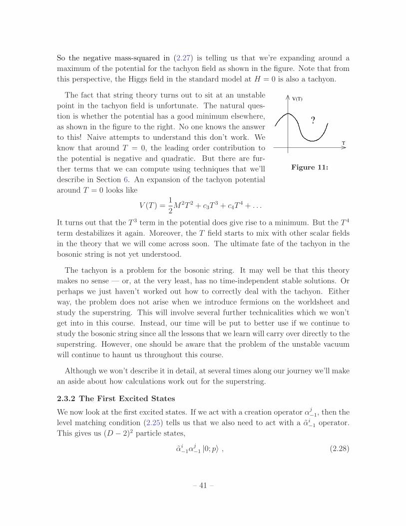
So the negative mass-squared in (2.27) is telling us that we’re expanding around a

maximum of the potential for the tachyon field as shown in the figure. Note that from

this perspective, the Higgs field in the standard model at H = 0 is also a tachyon.

The fact that string theory turns out to sit at an unstable

T

V(T)

?

Figure 11:

point in the tachyon field is unfortunate. The natural ques-

tion is whether the potential has a good minimum elsewhere,

as shown in the figure to the right. No one knows the answer

to this! Naive attempts to understand this don’t work. We

know that around T = 0, the leading order contribution to

the potential is negative and quadratic. But there are fur-

ther terms that we can compute using techniques that we’ll

describe in Section 6. An expansion of the tachyon potential

around T = 0 looks like

V (T ) =1

2M2T 2 + c

3

T 3 + c4

T 4 + . . .

It turns out that the T 3 term in the potential does give rise to a minimum. But the T 4

term destabilizes it again. Moreover, the T field starts to mix with other scalar fields

in the theory that we will come across soon. The ultimate fate of the tachyon in the

bosonic string is not yet understood.

The tachyon is a problem for the bosonic string. It may well be that this theory

makes no sense — or, at the very least, has no time-independent stable solutions. Or

perhaps we just haven’t worked out how to correctly deal with the tachyon. Either

way, the problem does not arise when we introduce fermions on the worldsheet and

study the superstring. This will involve several further technicalities which we won’t

get into in this course. Instead, our time will be put to better use if we continue to

study the bosonic string since all the lessons that we learn will carry over directly to the

superstring. However, one should be aware that the problem of the unstable vacuum

will continue to haunt us throughout this course.

Although we won’t describe it in detail, at several times along our journey we’ll make

an aside about how calculations work out for the superstring.

2.3.2 The First Excited States

We now look at the first excited states. If we act with a creation operator ↵j�1

, then the

level matching condition (2.25) tells us that we also need to act with a ↵i�1

operator.

This gives us (D � 2)2 particle states,

↵i�1

↵j�1

|0; pi , (2.28)

– 41 –

each of which has mass

M2 =4

↵0

✓1� D � 2

24

◆.

But now we seem to have a problem. Our states have space indices i, j = 1, . . . , D� 2.

The operators ↵i and ↵i each transform in the vector representation of SO(D � 2) ⇢SO(1, D�1) which is manifest in lightcone gauge. But ultimately we want these states

to fit into some representation of the full Lorentz SO(1, D � 1) group. That looks as

if it’s going to be hard to arrange. This is the first manifestation of the comment that

we made after equation (2.12): it’s tricky to see Lorentz invariance in lightcone gauge.

To proceed, let’s recall Wigner’s classification of representations of the Poincare

group. We start by looking at massive particles in R1,D�1. After going to the rest

frame of the particle by setting pµ = (p, 0, . . . , 0), we can watch how any internal

indices transform under the little group SO(D � 1) of spatial rotations. The upshot

of this is that any massive particle must form a representation of SO(D � 1). But the

particles described by (2.28) have (D � 2)2 states. There’s no way to package these

states into a representation of SO(D� 1) and this means that there’s no way that the

first excited states of the string can form a massive representation of the D-dimensional

Poincare group.

It looks like we’re in trouble. Thankfully, there’s a way out. If the states are massless,

then we can’t go to the rest frame. The best that we can do is choose a spacetime

momentum for the particle of the form pµ = (p, 0, . . . , 0, p). In this case, the particles

fill out a representation of the little group SO(D�2). This means that massless particles

get away with having fewer internal states than massive particles. For example, in four

dimensions the photon has two polarization states, but a massive spin-1 particle must

have three.

The first excited states (2.28) happily sit in a representation of SO(D�2). We learn

that if we want the quantum theory to preserve the SO(1, D � 1) Lorentz symmetry

that we started with, then these states will have to be massless. And this is only the

case if the dimension of spacetime is

D = 26 .

This is our first derivation of the critical dimension of the bosonic string.

Moreover, we’ve found that our theory contains a bunch of massless particles. And

massless particles are interesting because they give rise to long range forces. Let’s look

– 42 –

more closely at what massless particles the string has given us. The states (2.28) trans-

form in the 24⌦ 24 representation of SO(24). These decompose into three irreducible

representations:

traceless symmetric � anti-symmetric � singlet (=trace)

To each of these modes, we associate a massless field in spacetime such that the string

oscillation can be identified with a quantum of these fields. The fields are:

Gµ⌫(X) , Bµ⌫(X) , �(X) (2.29)

Of these, the first is the most interesting and we shall have more to say momentarily.

The second is an anti-symmetric tensor field which is usually called the anti-symmetric

tensor field. It also goes by the names of the “Kalb-Ramond field” or, in the language

of di↵erential geometry, the “2-form”. The scalar field is called the dilaton. These three

massless fields are common to all string theories. We’ll learn more about the role these

fields play later in the course.

The particle in the symmetric traceless representation of SO(24) is particularly in-

teresting. This is a massless spin 2 particle. However, there are general arguments,

due originally to Feynman and Weinberg, that any theory of interacting massless spin

two particles must be equivalent to general relativity2. We should therefore identify

the field Gµ⌫(X) with the metric of spacetime. Let’s pause briefly to review the thrust

of these arguments.

Why Massless Spin 2 = General Relativity

Let’s call the spacetime metric Gµ⌫(X). We can expand around flat space by writing

Gµ⌫ = ⌘µ⌫ + hµ⌫(X) .

Then the Einstein-Hilbert action has an expansion in powers of h. If we truncate to

quadratic order, we simply have a free theory which we may merrily quantize in the

usual canonical fashion: we promote hµ⌫ to an operator and introduce the associated

creation and annihilation operators aµ⌫ and a†µ⌫ . This way of looking at gravity is

anathema to those raised in the geometrical world of general relativity. But from a

particle physics language it is very standard: it is simply the quantization of a massless

spin 2 field, hµ⌫ .

2A very readable description of this can be found in the first few chapters of the Feynman Lectures

on Gravitation.

– 43 –

However, even on this simple level, there is a problem due to the indefinite signature

of the spacetime Minkowski metric. The canonical quantization relations of the creation

and annihilation operators are schematically of the form,

[aµ⌫ , a†⇢�] ⇠ ⌘µ⇢⌘⌫� + ⌘µ�⌘⌫⇢

But this will lead to a Hilbert space with negative norm states coming from acting with

time-like creation operators. For example, the one-graviton state of the form,

a†0i|0i (2.30)

su↵ers from a negative norm. This should be becoming familiar by now: it is the usual

problem that we run into if we try to covariantly quantize a gauge theory. And, indeed,

general relativity is a gauge theory. The gauge transformations are di↵eomorphisms.

We would hope that this saves the theory of quantum gravity from these negative norm

states.

Let’s look a little more closely at what the gauge symmetry looks like for small fluctu-

ations hµ⌫ . We’ve butchered the Einstein-Hilbert action and left only terms quadratic

in h. Including all the index contractions, we find

SEH =M2

pl

2

Zd4x

@µh

⇢⇢@⌫h

µ⌫ � @⇢hµ⌫@µh⇢⌫ +1

2@⇢hµ⌫@

⇢hµ⌫ � 1

2@µh

⌫⌫@

µh⇢⇢

�+ . . .

One can check that this truncated action is invariant under the gauge symmetry,

hµ⌫ �! hµ⌫ + @µ⇠⌫ + @⌫⇠µ (2.31)

for any function ⇠µ(X). The gauge symmetry is the remnant of di↵eomorphism invari-

ance, restricted to small deviations away from flat space. With this gauge invariance

in hand one can show that, just like QED, the negative norm states decouple from all

physical processes.

To summarize, theories of massless spin 2 fields only make sense if there is a gauge

symmetry to remove the negative norm states. In general relativity, this gauge symme-

try descends from di↵eomorphism invariance. The argument of Feynman and Weinberg

now runs this logic in reverse. It goes as follows: suppose that we have a massless, spin

2 particle. Then, at the linearized level, it must be invariant under the gauge symmetry

(2.31) in order to eliminate the negative norm states. Moreover, this symmetry must

survive when interaction terms are introduced. But the only way to do this is to ensure

that the resulting theory obeys di↵eomorpism invariance. That means the theory of

any interacting, massless spin 2 particle is Einstein gravity, perhaps supplemented by

higher derivative terms.

– 44 –

We haven’t yet shown that string theory includes interactions for hµ⌫ but we will

come to this later in the course. More importantly, we will also explicitly see how

Einstein’s field equations arise directly in string theory.

A Comment on Spacetime Gauge Invariance

We’ve surreptitiously put µ, ⌫ = 0, . . . , 25 indices on the spacetime fields, rather than

i, j = 1, . . . , 24. The reason we’re allowed to do this is because both Gµ⌫ and Bµ⌫ enjoy

a spacetime gauge symmetry which allows us to eliminate appropriate modes. Indeed,

this is exactly the gauge symmetry (2.31) that entered the discussion above. It isn’t

possible to see these spacetime gauge symmetries from the lightcone formalism of the

string since, by construction, we find only the physical states (although, by consistency

alone, the gauge symmetries must be there). One of the main advantages of pushing

through with the covariant calculation is that it does allow us to see how the spacetime

gauge symmetry emerges from the string worldsheet. Details can be found in Green,

Schwarz and Witten. We’ll also briefly return to this issue in Section 5.

2.3.3 Higher Excited States

We rescued the Lorentz invariance of the first excited states by choosing D = 26 to

ensure that they are massless. But now we’ve used this trick once, we still have to

worry about all the other excited states. These also carry indices that take the range

i, j = 1, . . . , D � 2 = 24 and, from the mass formula (2.26), they will all be massive

and so must form representations of SO(D � 1). It looks like we’re in trouble again.

Let’s examine the string at level N = N = 2. In the right-moving sector, we now

have two di↵erent states: ↵i�1

↵j�1

|0i and ↵i�2

|0i. The same is true for the left-moving

sector, meaning that the total set of states at level 2 is (in notation that is hopefully

obvious, but probably technically wrong)

(↵i�1

↵j�1

� ↵i�2

)⌦ (↵i�1

↵j�1

� ↵i�2

)|0; pi .

These states have mass M2 = 4/↵0. How many states do we have? In the left-moving

sector, we have,

1

2

(D � 2)(D � 1) + (D � 2) = 1

2

D(D � 1)� 1 .

But, remarkably, that does fit nicely into a representation of SO(D � 1), namely the

traceless symmetric tensor representation.

In fact, one can show that all excited states of the string fit nicely into SO(D � 1)

representations. The only consistency requirement that we need for Lorentz invariance

is to fix up the first excited states: D = 26.

– 45 –

Note that if we are interested in a fundamental theory of quantum gravity, then all

these excited states will have masses close to the Planck scale so are unlikely to be

observable in particle physics experiments. Nonetheless, as we shall see when we come

to discuss scattering amplitudes, it is the presence of this infinite tower of states that

tames the ultra-violet behaviour of gravity.

2.4 Lorentz Invariance Revisited

The previous discussion allowed to us to derive both the critical dimension and the

spectrum of string theory in the quickest fashion. But the derivation creaks a little in

places. The calculation of the Casimir energy is unsatisfactory the first time one sees

it. Similarly, the explanation of the need for massless particles at the first excited level

is correct, but seems rather cheap considering the huge importance that we’re placing

on the result.

As I’ve mentioned a few times already, we’ll shortly do better and gain some physical

insight into these issues, in particular the critical dimension. But here I would just like

to briefly sketch how one can be a little more rigorous within the framework of lightcone

quantization. The question, as we’ve seen, is whether one preserves spacetime Lorentz

symmetry when we quantize in lightcone gauge. We can examine this more closely.

Firstly, let’s go back to the action for free scalar fields (1.30) before we imposed

lightcone gauge fixing. Here the full Poincare symmetry was manifest: it appears as a

global symmetry on the worldsheet,

Xµ ! ⇤µ⌫X

⌫ + cµ (2.32)

But recall that in field theory, global symmetries give rise to Noether currents and

their associated conserved charges. What are the Noether currents associated to this

Poincare transformation? We can start with the translations Xµ ! Xµ + cµ. A quick

computation shows that the current is,

P↵µ = T@↵Xµ (2.33)

which is indeed a conserved current since @↵P↵µ = 0 is simply the equation of motion.

Similarly, we can compute the 1

2

D(D � 1) currents associated to Lorentz transforma-

tions. They are,

J↵µ⌫ = P↵

µX⌫ � P↵⌫ Xµ

It’s not hard to check that @↵J↵µ⌫ = 0 when the equations of motion are obeyed.

– 46 –

The conserved charges arising from this current are given by Mµ⌫ =Rd�J⌧

µ⌫ . Using

the mode expansion (1.36) for Xµ, these can be written as

Mµ⌫ = (pµx⌫ � p⌫xµ)� i1Xn=1

1

n

�↵⌫�n↵

µn � ↵µ

�n↵⌫n

�� i

1Xn=1

1

n

�↵⌫�n↵

µn � ↵µ

�n↵⌫n

�⌘ lµ⌫ + Sµ⌫ + Sµ⌫

The first piece, lµ⌫ , is the orbital angular momentum of the string while the remaining

pieces Sµ⌫ and Sµ⌫ tell us the angular momentum due to excited oscillator modes.

Classically, these obey the Poisson brackets of the Lorentz algebra. Moreover, if we

quantize in the covariant approach, the corresponding operators obey the commutation

relations of the Lorentz Lie algebra, namely

[M⇢�,M⌧⌫ ] = ⌘�⌧M⇢⌫ � ⌘⇢⌧M�⌫ + ⌘⇢⌫M�⌧ � ⌘�⌫M⇢⌧

However, things aren’t so easy in lightcone gauge. Lorentz invariance is not guaranteed

and, in general, is not there. The right way to go about looking for it is to make sure

that the Lorentz algebra above is reproduced by the generators Mµ⌫ . It turns out that

the smoking gun lies in the commutation relation,

[Mi�,Mj�] = 0

Does this equation hold in lightcone gauge? The problem is that it involves the op-

erators p� and ↵�n , both of which are fixed by (2.17) and (2.18) in terms of the other

operators. So the task is to compute this commutation relation [Mi�,Mj�], given the

commutation relations (2.21) for the physical degrees of freedom, and check that it van-

ishes. To do this, we re-instate the ordering ambiguity a and the number of spacetime

dimension D as arbitrary variables and proceed.

The part involving orbital angular momenta li� is fairly straightforward. (Actually,

there’s a small subtlety because we must first make sure that the operator lµ⌫ is Hermi-

tian by replacing xµp⌫ with 1

2

(xµp⌫ + p⌫xµ)). The real di�culty comes from computing

the commutation relations [Si�, Sj�]. This is messy3. After a tedious computation,

one finds,

[Mi�,Mj�] =2

(p+)2

Xn>0

✓D � 2

24� 1

�n+

1

n

a� D � 2

24

�◆(↵i

�n↵jn � ↵j

�n↵in) + (↵ $ ↵)

3The original, classic, paper where lightcone quantization was first implemented is Goddard, Gold-

stone, Rebbi and Thorn “Quantum Dynamics of a Massless Relativistic String”, Nucl. Phys. B56

(1973). A pedestrian walkthrough of this calculation can be found in the lecture notes by Gleb Aru-

tyunov. A link is given on the course webpage.

– 47 –

The right-hand side does not, in general, vanish. We learn that the relativistic string

can only be quantized in flat Minkowski space if we pick,

D = 26 and a = 1 .

2.5 A Nod to the Superstring

We won’t provide details of the superstring in this course, but will pause occasionally

to make some pertinent comments. Although what follows is nothing more than a list

of facts, it will hopefully be helpful in orienting you when you do come to study this

material.

The key di↵erence between the bosonic string and the superstring is the addition of

fermionic modes on its worldsheet. The resulting worldsheet theory is supersymmetric.

(At least in the so-called Neveu-Schwarz-Ramond formalism). Hence the name “super-

string”. Applying the kind of quantization procedure we’ve discussed in this section,

one finds the following results:

• The critical dimension of the superstring is D = 10.

• There is no tachyon in the spectrum.

• The massless bosonic fields Gµ⌫ , Bµ⌫ and � are all part of the spectrum of the

superstring. In this context, Bµ⌫ is sometimes referred to as the Neveu-Schwarz

2-form. There are also massless spacetime fermions, as well as further massless

bosonic fields. As we now discuss, the exact form of these extra bosonic fields

depends on exactly what superstring theory we consider.

While the bosonic string is unique, there are a number of discrete choices that one

can make when adding fermions to the worldsheet. This gives rise to a handful of

di↵erent perturbative superstring theories. (Although later developments reveal that

they are actually all part of the same framework which sometimes goes by the name of

M-theory). The most important of these discrete options is whether we add fermions in

both the left-moving and right-moving sectors of the string, or whether we choose the

fermions to move only in one direction, usually taken to be right-moving. This gives

rise to two di↵erent classes of string theory.

• Type II strings have both left and right-moving worldsheet fermions. The result-

ing spacetime theory in D = 10 dimensions has N = 2 supersymmetry, which

means 32 supercharges.

• Heterotic strings have just right-moving fermions. The resulting spacetime theory

has N = 1 supersymmetry, or 16 supercharges.

– 48 –

In each of these cases, there is then one further discrete choice that we can make.

This leaves us with four superstring theories. In each case, the massless bosonic fields

include Gµ⌫ , Bµ⌫ and � together with a number of extra fields. These are:

• Type IIA: In the type II theories, the extra massless bosonic excitations of the

string are referred to as Ramond-Ramond fields. For Type IIA, they are a 1-

form Cµ and a 3-form Cµ⌫⇢. Each of these is to be thought of as a gauge field.

The gauge invariant information lies in the field strengths which take the form

F = dC.

• Type IIB: The Ramond-Ramond gauge fields consist of a scalar C, a 2-form Cµ⌫

and a 4-form Cµ⌫⇢�. The 4-form is restricted to have a self-dual field strength:

F5

= ?F5

. (Actually, this statement is almost true...we’ll look a little closer at

this in Section 7.3.3).

• Heterotic SO(32): The heterotic strings do not have Ramond-Ramond fields.

Instead, each comes with a non-Abelian gauge field in spacetime. The heterotic

strings are named after the gauge group. For example, the Heterotic SO(32)

string gives rise to an SO(32) Yang-Mills theory in ten dimensions.

• Heterotic E8

⇥E8

: The clue is in the name. This string gives rise to an E8

⇥E8

Yang-Mills field in ten-dimensions.

It is sometimes said that there are five perturbative superstring theories in ten dimen-

sions. Here we’ve only mentioned four. The remaining theory is called Type I and

includes open strings moving in flat ten dimensional space as well as closed strings.

We’ll mention it in passing in the following section.

– 49 –