2. MANIPULATOR KINEMATICS - ene.ttu.ee · PDF fileManipulators with parallel kinematics Kinematics of mobile robots 2.1. Position vectors and their transformation

2. MANIPULATOR KINEMATICS

Position vectors and their transformations Direct and inverse kinematics of manipulators Transformation of velocity and torque vectors Classification of kinematical chains of manipulator Cartesian, polar cylindrical and spherical and angular coordinates of manipulators Multilink manipulators and manipulators with flexible links Manipulators with parallel kinematics Kinematics of mobile robots

2.1. Position vectors and their transformation Manipulator kinematics is the field of science that investigates the motion of manipulator links without regard to the forces that cause it. In that case the motion is determined with trajectory, i.e. positions, velocity, acceleration, jerk and other higher derivative components.

PAr

The location of a point A in Cartesian coordinates {A} is determined by vector (Fig 2.1), the individual element of which are projections to the three orthogonal axes of coordinates x, y, z, respectively. The projections px, py and pz can be considered as three orthogonal vectors.

.⎥⎥⎥

⎦

⎤

⎢⎢⎢

⎣

⎡=

z

y

xA

ppp

Pr

(2.1)

The orientation of a body in Cartesian space {A} is determined by three unit vectors

BBB zyx rrr ,, that are attached to the body. These orthogonal unit vectors form the Cartesian coordinate system {B} that can be called body coordinates {B}. Therefore, the orientation of a body in space coordinates can be described by the rotation of body coordinates {B} relative to the reference coordinates {A}. The unit vector Bxr can be described in Cartesian space coordinates {A} with three projections to coordinate axes xA, yA, zA. In the same way, other unit vectors Byr Bzr and can be described.

{A}

px

x

y

z

PA

py

pz

OA

Figure 2.1. Position vector of a point in Cartesian coordinates

32

Generally

⎥⎥⎥

⎦

⎤

⎢⎢⎢

⎣

⎡

=

BZ

BY

BX

BA

xxx

Xr

. (2.2)

⎥⎥⎥

⎦

⎤

⎢⎢⎢

⎣

⎡

=

BZ

BY

BX

BA

yyy

Yr

⎥⎥⎥

⎦

⎤

⎢⎢⎢

⎣

⎡

=

BZ

BY

BX

BA

zzz

Zr

BAZr

Three vectors: , and BA Xr

BAYr

will form the rotation matrix , which describes the orientation of coordinates {B} relative to coordinates {A}.

BAR

[ .,, BA

BA

BA

BZ

BZ

BZ

BY

BY

BY

BX

BX

BX

AB ZYX

zyxzyxzyx

Rrrr

=⎥⎥⎥

⎦

⎤

⎢⎢⎢

⎣

⎡

= ]

}

(2.3)

The position of coordinates {B} relative to coordinates {A} (Fig. 2.2) is defined by the position vector of the origin of coordinates {B} in coordinates {A} and rotation matrix

BO

APr

B

AR.

{ } { .,B BOAA

B PRr

= (2.4)

PBr

The position vector in translated coordinates {B} relative to coordinates {A} (Fig. 2.3) is defined by the sum of two vectors

.BOABA PPPrrr

+= (2.5)

PBr

The position vector in rotated coordinates {B} relative to coordinates {A} is defined by the rotation matrix . In this case the position vector PA

rRA

B is determined as the scalar product of the rotation matrix and the position vector PB

rBAR (2.6).

{A} zA

xB

OA

APBO

{B}

xA

yB

zB

yA

OB

Figure 2.2 Determination of manipulator gripper or tool orientation

33

xA

{Α}

APBO AP

BP

OB

zB

yB

xB

zA

yA

{Β}

OA

Figure 2.3 Position vectors in translated coordinates {A} and {B}

.PRP BAB

Arr

⋅= (2.6) The rotation matrix describes the rotation of coordinates {B} relative to coordinates {A}. We can use the rotation matrix to describe inversely coordinates {A} relative to coordinates {B}. This transformation will be described by the rotation matrix . It is known from the course of linear algebra that the inverse of matrix with orthonormal columns is equal to its transpose. The transpose of the matrix is defined by the change of elements of rows and columns.

RAB

RBA

.1 TA

BAB

BA RRR == − (2.7) The program MathCAD Symbolics helps us to calculate and we can easily demonstrate that the inverse of the rotation matrix is equal to its transpose. , because the nominator of elements in rotation matrix

TAB

AB RR =−1

1−R is equal to one.

Rcos α( )sin α( )

0

sin α( )−

cos α( )0

0

0

1

⎛⎜⎜⎝

⎞⎟⎟⎠

:=

RTcos α( )sin α( )−

0

sin α( )cos α( )

0

0

0

1

⎛

α

⎜⎜⎜⎝

⎞⎟⎟⎟⎠

→

R 1−

cos α( )cos α( )2 sin α( )2

+( )sin α( )−

cos α( )2 sin α( )2+( )0

sin α( )cos α( )2 sin α( )2

+( )cos α( )

cos α( )2 sin α( )2+( )0

0

0

1

⎡⎢⎢⎢⎢⎢⎣

⎤⎥⎥⎥⎥⎥⎦

→

34

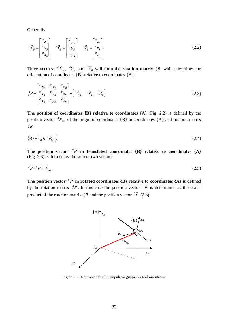
The matrix with orthogonal elements the norm of which is equal to 1 (orthogonal unit vectors) is called orthonormal. The transposed matrix is the matrix with transposed rows and columns. The inverse matrix is calculated by the formula

),(det

11jiR

RR =− (2.8)

where Rji is an adjunct matrix. The inverse matrix of the orthonormal matrix is equal to the transposed matrix. Because the rotation matrix is orthonormal, its inverse matrix can be found as its transpose. The product of the matrix and its inverse gives a unit matrix. The unit matrix has diagonal elements equal to 1, and all other elements equal to 0. The scalar product of matrixes can be calculated by using the formula:

c a bik ij ikj

n

= ⋅=∑ ( )

1

. (2.9)

The formula can be used for the calculation of product 2.6. In this case the matrix aij is the rotation matrix and bjk is the position vector PB

rPAr

. The result cik is the position vector , where (i = 1...3; j = 1...3; k = 1).

PBr

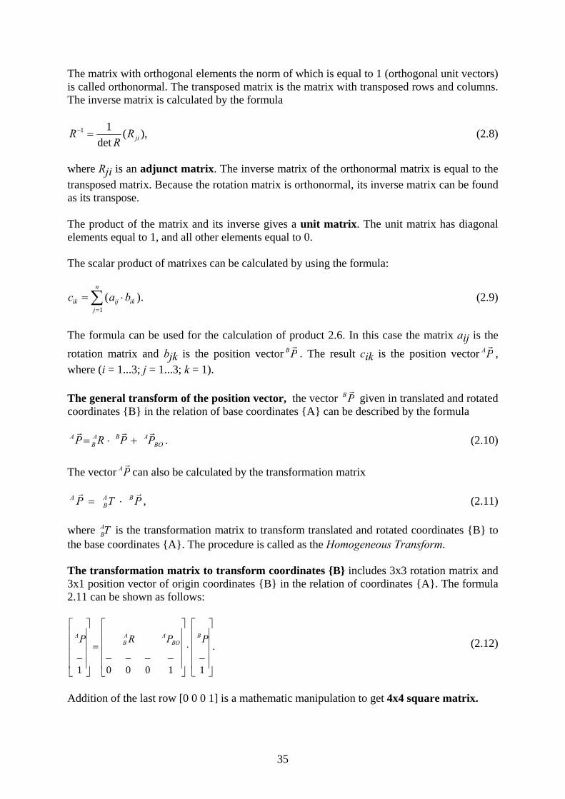
The general transform of the position vector, the vector given in translated and rotated coordinates {B} in the relation of base coordinates {A} can be described by the formula

.BOABA

BA PPRP

rrr+⋅= (2.10)

PAr

The vector can also be calculated by the transformation matrix

,PTP BAB

Arr

⋅= (2.11) where B is the transformation matrix to transform translated and rotated coordinates {B} to the base coordinates {A}. The procedure is called as the Homogeneous Transform.

AT

The transformation matrix to transform coordinates {B} includes 3x3 rotation matrix and 3x1 position vector of origin coordinates {B} in the relation of coordinates {A}. The formula 2.11 can be shown as follows:

.

1_

1000____

1_

⎥⎥⎥⎥

⎦

⎤

⎢⎢⎢⎢

⎣

⎡

⋅

⎥⎥⎥⎥

⎦

⎤

⎢⎢⎢⎢

⎣

⎡

=

⎥⎥⎥⎥

⎦

⎤

⎢⎢⎢⎢

⎣

⎡PPRP B

BOAA

BA

(2.12)

Addition of the last row [0 0 0 1] is a mathematic manipulation to get 4x4 square matrix.

35

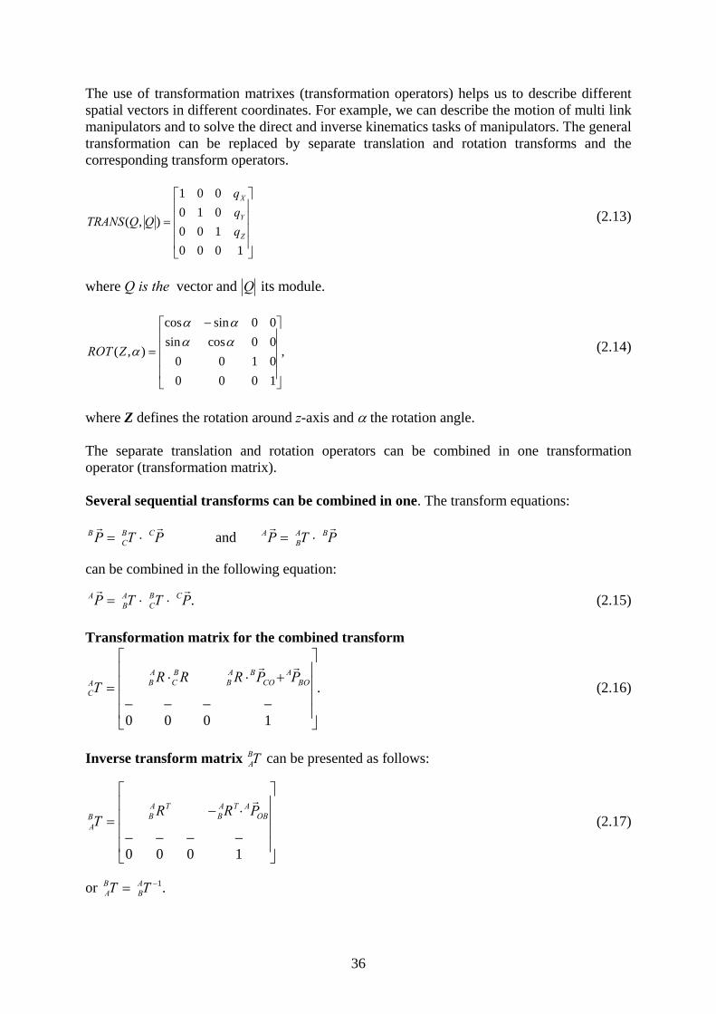
The use of transformation matrixes (transformation operators) helps us to describe different spatial vectors in different coordinates. For example, we can describe the motion of multi link manipulators and to solve the direct and inverse kinematics tasks of manipulators. The general transformation can be replaced by separate translation and rotation transforms and the corresponding transform operators.

⎥⎥⎥⎥

⎦

⎤

⎢⎢⎢⎢

⎣

⎡

=

1000100010001

),(Z

Y

X

qqq

QQTRANS (2.13)

where Q is the vector and its module. Q

,

1000010000cossin00sincos

),(

⎥⎥⎥⎥

⎦

⎤

⎢⎢⎢⎢

⎣

⎡ −

=αααα

αZROT (2.14)

where Z defines the rotation around z-axis and α the rotation angle. The separate translation and rotation operators can be combined in one transformation operator (transformation matrix). Several sequential transforms can be combined in one. The transform equations:

PTP CBC

Brr

⋅= PTP BAB

Arr

⋅= and can be combined in the following equation:

.PTTP CBC

AB

Arr

⋅⋅= (2.15) Transformation matrix for the combined transform

.

1000____

⎥⎥⎥⎥

⎦

⎤

⎢⎢⎢⎢

⎣

⎡+⋅⋅

= BOA

COBA

BBC

ABA

C

PPRRRT

rr

(2.16)

Inverse transform matrix can be presented as follows: A

BT

⎥⎥⎥⎥

⎦

⎤

⎢⎢⎢⎢

⎣

⎡⋅−

=

1000____

OBATA

BTA

BBA

PRRT

r

(2.17)

or .1−= TT AB

BA

36

The transformation matrix AB is not orthonormal (consisting only of orthogonal unit vectors)

and therefore its inverse matrix is not equal to the transposed matrix. T

By solving transform equations it is possible to find solutions for any unknown transform if sufficient transform conditions exist. For example, if we know the conditions

TTT AD

EA

ED ⋅= and TTTT C

DBC

EB

ED ⋅⋅=

then .TTTTT CD

BC

EB

AD

EA ⋅⋅==

Consequently,

.11 −− ⋅⋅= TTTT CD

AD

EB

BC (2.18) Euler angles. The rotation matrix is not the only way to define the orientation of a body. We can define the orientation of a body also by three independent angles. The nine elements of the rotation matrix are mutually dependent and there are six conditions, including three conditions for the longitude of the unit vector

;1ˆ =X ;1ˆ =Y ;1ˆ =Z (2.19) and three conditions for their orthogonal location exist.

;0ˆˆ =⋅YX (2.20)

;0ˆˆ =⋅ZX 0ˆˆ =⋅ZY

The following calculation using the MathCAD program illustrates the issue of scalar or dot product and cross product of orthogonal vectors. The dot product of two orthogonal or parallel vectors with magnitude 5 gives

0

5

0

⎛⎜⎜⎜⎝

⎞⎟⎟⎟⎠

5

0

0

⎛⎜⎜⎜⎝

⎞⎟⎟⎟⎠

⋅ 0=

5

0

0

⎛⎜⎜⎜⎝

⎞⎟⎟⎟⎠

5

0

0

⎛⎜⎜⎜⎝

⎞⎟⎟⎟⎠

⋅ 25=

αsin⋅⋅⋅=× banba rrrThe cross product of the same vectors gives

5

0

0

⎛⎜⎜⎜⎝

⎞⎟⎟⎟⎠

0

5

0

⎛⎜⎜⎜⎝

⎞⎟⎟⎟⎠

×

0

0

25

⎛⎜⎜⎜⎝

⎞⎟⎟⎟⎠

=

5

0

0

⎛⎜⎜⎜⎝

⎞⎟⎟⎟⎠

5

0

0

⎛⎜⎜⎜⎝

⎞⎟⎟⎟⎠

×

0

0

0

⎛⎜⎜⎜⎝

⎞⎟⎟⎟⎠

=

,

br

where the resultant vector is orthogonal to the unit vector arnr and . Hence, the scalar or dot product of two orthogonal vectors is equal to zero, but their cross product is an orthogonal vector the magnitude of which equals the scalar product of two magnitudes. To conclude we can declare that any rotation of the coordinate system can be described by three independent variables. Mostly three independent angles: roll, pitch and yaw angles are used in this case (Fig. 2.4). The rotation angle on yz-plane if rotation happens around x axis is defined by the roll angle α, the rotation angle on xz-plane if rotation happens around y axis is

37

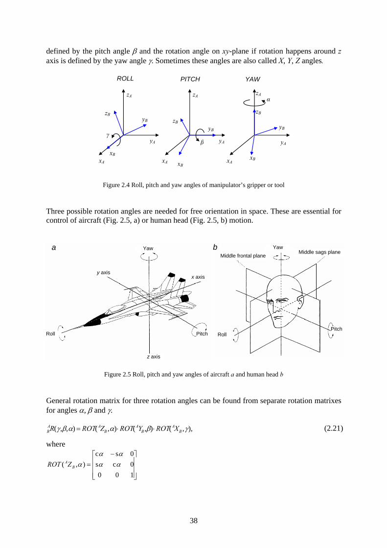
defined by the pitch angle β and the rotation angle on xy-plane if rotation happens around z axis is defined by the yaw angle γ. Sometimes these angles are also called X, Y, Z angles.

ROLL PITCH YAW

zB

xB

yB

yA

zA

xA

zB

xB

yB

yA

zA

xA

zB

xB

yB

yA

zA

xA

β

α

γ

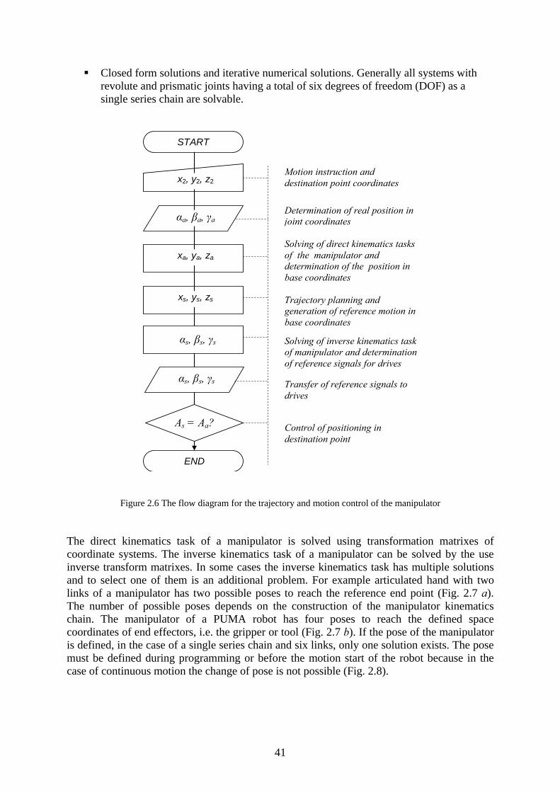
Figure 2.4 Roll, pitch and yaw angles of manipulator’s gripper or tool Three possible rotation angles are needed for free orientation in space. These are essential for control of aircraft (Fig. 2.5, a) or human head (Fig. 2.5, b) motion.

Figure 2.5 Roll, pitch and yaw angles of aircraft a and human head b

General rotation matrix for three rotation angles can be found from separate rotation matrixes for angles α, β and γ. BA A

BA

BA

BR ROT Z ROT Y ROT X( , , ) ( , ) ( , ) ( , ),γ β α α β γ= ⋅ ⋅ (2.21) where

⎥⎥⎥

⎦

⎤

⎢⎢⎢

⎣

⎡ −=

1000cs0sc

),( αααα

αBAZROT

Middle frontal planeMiddle sags plane

Roll Pitch

Yaw

Roll

z axis

y axis x axis

Yaw

Pitch

a b

38

⎥⎥⎥

⎦

⎤

⎢⎢⎢

⎣

⎡

−=

ββ

βββ

c0s010

s0c),( B

AYROT

⎥⎥⎥

⎦

⎤

⎢⎢⎢

⎣

⎡−=γγγγγ

cs0sc0001

),( BAXROT

In this case and also in future examples the first letters s and c are used instead of functions sine and cosine to reduce the formula. General rotation matrix for angles α, β and γ is

⎥⎥⎥

⎦

⎤

⎢⎢⎢

⎣

⎡

⋅⋅−⋅−⋅⋅⋅+⋅⋅⋅⋅+⋅⋅⋅−⋅⋅⋅

=γβγββ

γαγβαγαγβαβαγαγβαγαγβαβα

αβγccscs

sccssccssscssscsccsscccc

),,(RAB

(2.22)

The MathCAD program is very convenient for the calculation of matrix products. For symbolic calculations the toolbox MathCAD Symbolic can be used. The following example shows the use of MathCAD Symbolic toolbox for the calculation of matrixes product using symbolic elements.

T1

cos α( )sin α( )

0

0

sin α( )−

cos α( )0

0

0

0

1

0

x

y

z

1

⎛⎜⎜⎜⎜⎝

⎞⎟⎟⎟⎟⎠

:=

T2

cos β( )0

sin β( )0

sin β( )−

0

cos β( )0

0

1

0

0

a

0

1

⎛

z

h

⎜⎜⎜⎜⎝

⎞⎟⎟⎟⎟⎠

:=

T T1:=

T

cos α( ) cos β( )⋅

sin α( ) cos β( )⋅

sin β( )0

cos α( )− sin β( )⋅

sin α( )− sin β( )⋅

cos β( )0

sin α( )−

cos α( )0

0

cos α( ) a⋅ x+

sin α( ) a⋅ y+

h z+

1

⎛

h

T2⋅T2

⎞⎜ ⎟⎜⎜

⎟⎟→

⎜ ⎟⎝ ⎠

The transformation matrix written in the symbolic mode can be used for solving tasks of inverse kinematics. In this case the links of rotation angles α and β will be determined if the gripper positioning coordinates x, y and z are known.

39

2.2. Description of manipulator kinematics Control procedure of a robot includes several sequential steps to realize the program instruction and reference motion between a given starting and a destination positioning point (x , y2 2, z ) in a robot’s working envelope. Generally these steps are as follows: 2 1. Detection of signals from position sensors located on the drive motor shaft and

determination of rotation angles (e.g. α , βa a, γa) of manipulator links in the joint coordinate system.

2. Calculation of the real location of the manipulator gripper or the tool in the base or world Cartesian coordinate system x , y , za a a, i.e. solving the direct kinematics task of the manipulator using angles (αa, β , γ ) in joint coordinates. a a

3. Comparison of the real position with the given motion destination point location in the base or world coordinates; planning of motion trajectory between the start and destination points in a robot’s working envelope space; determination of reference time diagrams for position, velocity, acceleration and jerk of manipulator gripper or tool, using linear or circular interpolation for trajectory generation.

4. Determination of motion time dependent reference coordinates in the Cartesian coordinate system (projections x , y , z ). r r r

5. Determination of motion time dependent joint reference coordinates (α , β , γr r r), i.e. solving the inverse kinematics tasks of the manipulator and transfer of the reference signals to manipulator joint drives.

6. Cyclic repeating of steps 1…5 and stopping the motion in the destination positioning point.

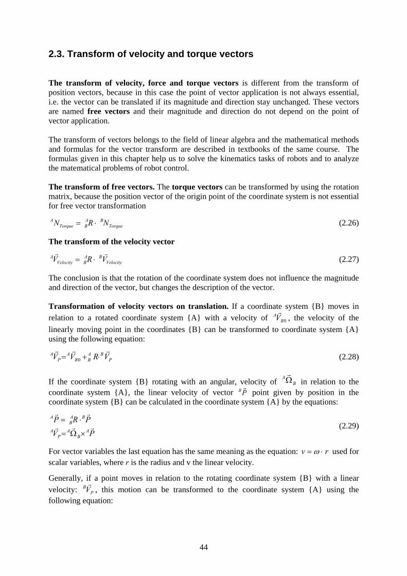
The flow diagram for the trajectory and motion control of manipulator is shown in Fig. 2.6. Direct kinematics of a manipulator To solve a direct kinematics task of a manipulator, the position of the gripper or the tool centre point and gripper or tool orientation coordinates in the base or world coordinates are calculated if the joint angles measured by drive sensors are known in joint coordinates. In other words, the gripper or tool location is calculated according to the measured angles of manipulator joints (links). Inverse kinematics of a manipulator To solve an inverse kinematics task of a manipulator, the location of all manipulator joints (links) in joint coordinates is calculated if the gripper or tool reference position and orientation angles are calculated by the trajectory planner in the base or world Cartesian coordinates. Methods for solving direct kinematics tasks

Geometric method (using basic formulas of geometry and trigonometry) Matrix method (using transformation matrixes of coordinate systems)

Methods for solving of inverse kinematics tasks

Definition of manipulator joints relative locations (pose) if multiple solutions exist.

40

Closed form solutions and iterative numerical solutions. Generally all systems with revolute and prismatic joints having a total of six degrees of freedom (DOF) as a single series chain are solvable.

Motion instruction and destination point coordinates

Determination of real position in joint coordinates Solving of direct kinematics tasks of the manipulator and determination of the position in base coordinates Trajectory planning and generation of reference motion in base coordinates Solving of inverse kinematics task of manipulator and determination of reference signals for drives

Transfer of reference signals to drives

Control of positioning in destination point

START

x2, y2, z2

αa, βa, γa

xa, ya, za

xs, ys, zs

αs, βs, γs

αs, βs, γs

As = Aa?

END

Figure 2.6 The flow diagram for the trajectory and motion control of the manipulator The direct kinematics task of a manipulator is solved using transformation matrixes of coordinate systems. The inverse kinematics task of a manipulator can be solved by the use inverse transform matrixes. In some cases the inverse kinematics task has multiple solutions and to select one of them is an additional problem. For example articulated hand with two links of a manipulator has two possible poses to reach the reference end point (Fig. 2.7 a). The number of possible poses depends on the construction of the manipulator kinematics chain. The manipulator of a PUMA robot has four poses to reach the defined space coordinates of end effectors, i.e. the gripper or tool (Fig. 2.7 b). If the pose of the manipulator is defined, in the case of a single series chain and six links, only one solution exists. The pose must be defined during programming or before the motion start of the robot because in the case of continuous motion the change of pose is not possible (Fig. 2.8).

41

Figure 2.7 Different poses of an articulated robot hand a, and manipulator of PUMA robot b if end effector coordinates are referred to

o

o

A1

A2L12

0 -x x

y

A1

A2 o

o

-x x0

y

Figure 2.8 Example of linear motion using articulated robot hand and impossible change of pose during this motion

To solve the inverse kinematics task of a manipulator, the roll, pitch and jaw angles of robot hand must be calculated using numerical values of given rotation matrix elements. If the rotation matrix has numerical elements rij

⎥⎥⎥

⎦

⎤

⎢⎢⎢

⎣

⎡=

333231

232221

131211

rrrrrrrrr

RAB (2.23)

and if we compare matrixes 2.22 and 2.23 and their elements, the angles of the orientation of the coordinate system can be calculated as follows:

42

)cos/,cos/(2tanarc)(2tanarc

)cos/,cos/(2tan

1121

221

211,31

3332

ββαβ

ββγ

rrrrr

rrA

=

+−=

=

(2.24)

where arctan2(rij) is the function of two arguments (y, x). For example, arctan2(2, 2) = 45°. Inverse kinematics equations can be solved using the MathCAD program and its operators Given and Find α 0:= β 0:= r1 6:= r2 4:=

Givencos α( ) cos β( )⋅ sin α( ) sin β( )⋅−( ) r2⋅ cos α( )( ) r1⋅+ 6

sin α( ) cos β( )⋅ cos α( ) sin β( )⋅+( ) r2⋅ sin α( )( ) r1⋅+ 4

α

β

⎛⎜⎝

⎞⎟⎠

Find α β,( ):=

α 0→

β 12π⋅→

The inverse kinematics equations are often transcendental equations, i.e. these equations have a solution that can not be described analytically with the help of known mathematical expressions. The transcendental equations can be solved numerically. The other way to solve the transcendental equations is using supplementary auxiliary functions and substitute variables. The trigonometric functions can be replaced with new algebraic functions and a new variable u.

( )

2

2

2

12sin

11cos

2/tan

uuuu

u

+=

+−

=

=

α

α

α

(2.25)

After that substitution, the transcendental equations are transformed to polynomials that have an analytical solution.

43

2.3. Transform of velocity and torque vectors The transform of velocity, force and torque vectors is different from the transform of position vectors, because in this case the point of vector application is not always essential, i.e. the vector can be translated if its magnitude and direction stay unchanged. These vectors are named free vectors and their magnitude and direction do not depend on the point of vector application. The transform of vectors belongs to the field of linear algebra and the mathematical methods and formulas for the vector transform are described in textbooks of the same course. The formulas given in this chapter help us to solve the kinematics tasks of robots and to analyze the matematical problems of robot control. The transform of free vectors. The torque vectors can be transformed by using the rotation matrix, because the position vector of the origin point of the coordinate system is not essential for free vector transformation

TorqueBA

BTorqueA NRN ⋅= (2.26)

The transform of the velocity vector

VelocityBA

BVelocityA VRV

rr⋅= (2.27)

The conclusion is that the rotation of the coordinate system does not influence the magnitude and direction of the vector, but changes the description of the vector. Transformation of velocity vectors on translation. If a coordinate system {B} moves in relation to a rotated coordinate system {A} with a velocity of 0B

AVr

, the velocity of the linearly moving point in the coordinates {B} can be transformed to coordinate system {A} using the following equation:

PBA

BBA

PA VRVV

rrr⋅+= 0 (2.28)

BAΩr

If the coordinate system {B} rotating with an angular, velocity of in relation to the coordinate system {A}, the linear velocity of vector PB

r point given by position in the

coordinate system {B} can be calculated in the coordinate system {A} by the equations:

PV

PRPA

BA

PA

BAB

A

rrr

rr

×Ω=

⋅= (2.29)

rv ⋅= ωFor vector variables the last equation has the same meaning as the equation: used for scalar variables, where r is the radius and v the linear velocity. Generally, if a point moves in relation to the rotating coordinate system {B} with a linear velocity: P

BVr

, this motion can be transformed to the coordinate system {A} using the following equation:

44

( ) PVV AB

AP

BAP

Arrrr

×Ω+= or (2.30)

PRVRV BABB

AP

BABP

Arrrr

⋅×Ω+⋅= (2.31) If the coordinate system {B} rotates and translates simultaneously the transformation of the velocity vector can be done by equation (2.32) similar to (2.31), but in this case the velocity vector of the origin point of coordinates {B} must be added.

PRVRVV BABB

AP

BABB

AP

Arrrrr

⋅×Ω+⋅+= 0 (2.32) Velocities of manipulator links The planar manipulator on the xy-plane is shown in Fig. 2.9. The stationary base coordinates of the manipulator are x0y0. Around the origin of coordinates (point O) rotates link 1 having longitude L . The second link has longitude L1 2 and is connected with the revolute joint to link 1. The relative rotation angles of links are α and α1 2. The angular velocity is the derivative of angular position. Consequently

222

111

ωαα

ωαα

==

==

&

&

dtddt

d

(2.33)

The angular velocities of links in the stationary base coordinates if rotating around z-axis are

⎥⎥⎥

⎦

⎤

⎢⎢⎢

⎣

⎡=Ω

1

10 0

0

ω

r

⎥⎥⎥

⎦

⎤

⎢⎢⎢

⎣

⎡

+=Ω

21

20 0

0

ωω

r2

03

0 Ω=Ωrr

(2.34)

y3

α1

α2

L1

L2

x3

y2

x2

y0 y1 x1

x0OV1 = 0

V2

V3

Figure 2.9 Planar articulated hand of the manipulator The linear velocity vector of the origin point of the coordinate system is defined by projections of the velocity vector to the corresponding axes of the coordinate system.

45

⎥⎥⎥

⎦

⎤

⎢⎢⎢

⎣

⎡=

000

11Vr

(2.35)

⎥⎥⎥

⎦

⎤

⎢⎢⎢

⎣

⎡=

0cossin

211

211

22 αω

αωLL

Vr

(⎥⎥⎥

⎦

⎤

⎢⎢⎢

⎣

⎡++=

0cos

sin

212211

211

33 ωωαω

αωLL

LVr

)

The manipulator has the following rotation and translation matrixes:

⎥⎥⎥

⎦

⎤

⎢⎢⎢

⎣

⎡ −=

10000

11

1101 cs

scR (2.36)

⎥⎥⎥

⎦

⎤

⎢⎢⎢

⎣

⎡ −=

10000

22

2212 cs

scR

⎥⎥⎥

⎦

⎤

⎢⎢⎢

⎣

⎡=

100010001

23 R

and

⎥⎥⎥⎥

⎦

⎤

⎢⎢⎢⎢

⎣

⎡ −

=

100001000000

11

11

01

cssc

T (2.37)

⎥⎥⎥⎥

⎦

⎤

⎢⎢⎢⎢

⎣

⎡ −

=

1000010000

0

22

122

12

csLsc

T

⎥⎥⎥⎥

⎦

⎤

⎢⎢⎢⎢

⎣

⎡

=

100001000010

001 2

23

L

T

The summary rotation matrix is

⎥⎥⎥

⎦

⎤

⎢⎢⎢

⎣

⎡ −=⋅⋅=

10000

1212

121223

12

01

03 cs

scRRRR (2.38)

where

( )21cos αα +212112 ssccc −= = ( )21sin αα +.212112 sccss += =

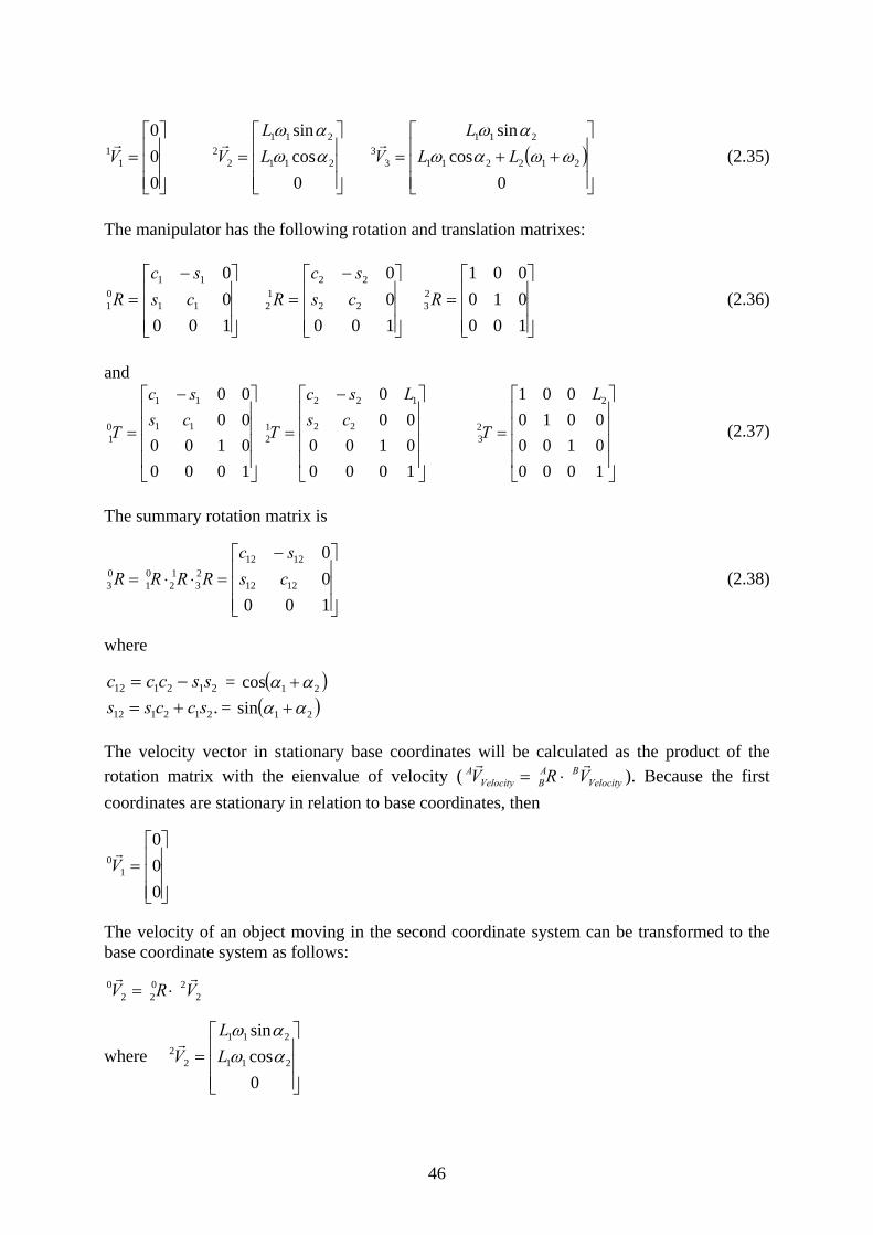
The velocity vector in stationary base coordinates will be calculated as the product of the rotation matrix with the eienvalue of velocity ( Velocity

BABVelocity

A VRVrr

⋅= ). Because the first coordinates are stationary in relation to base coordinates, then

⎥⎥⎥

⎦

⎤

⎢⎢⎢

⎣

⎡=

000

10Vr

The velocity of an object moving in the second coordinate system can be transformed to the base coordinate system as follows:

220

220 VRV

rr⋅=

where ⎥⎥⎥

⎦

⎤

⎢⎢⎢

⎣

⎡=

0cossin

211

211

22 αω

αωLL

Vr

46

and (2.39)

( )( )

⎥⎥⎥

⎦

⎤

⎢⎢⎢

⎣

⎡−=

0cossin

111

111

20 αω

αωLL

Vr

(⎥⎥⎥

⎦

⎤

⎢⎢⎢

⎣

⎡++=

0cos

sin

212211

211

33 ωωαω

αωLL

LVr

) (2.40)

( ) ( )[ ]( ) ([

⎥⎥⎥

⎦

⎤

⎢⎢⎢

⎣

⎡+++++−−

=0

coscossinsin

21212111

21212111

30 ααωωαω

ααωωαωLLLL

Vr

330

330 VRV

rr⋅= )] (2.41)

The solution can be easily found with the help of theMathCAD Symbolic program.

MathCAD calculates

Using the operator Simplify we get the following matrix expression:

Jacobian matrixes or Jacobians are used to describe of multidimensional derivatives of vectors. Because the velocity vector is the time related derivative of the position vector, the velocity vectors can be found using Jacobians. In the case of the six coordinate (six links) manipulator the Jacobian is a matrix with dimensions 6 x 6. The Jacobian of the manipulator with two coordinates (see Fig. 2.11) has dimensions 2 x 2.

Ω⋅=rr

JV 00 Jacobian matrix consists of components of linear velocity vectors ω and ω1 2. For previously described vectors ja 3

3Vr

30Vr

(⎥⎥⎥

⎦

⎤

⎢⎢⎢

⎣

⎡++=

0cos

sin

212211

211

33 ωωαω

αωLL

LVr

) and ( ) ( )[ ]( ) ([ ]

⎥⎥⎥

⎦

⎤

⎢⎢⎢

⎣

⎡+++++−−

=0

coscossinsin

21212111

21212111

30 ααωωαω

ααωωαωLLLL

Vr

)

the following Jacobians or Jacobian matrixes can be found:

47

( ) ⎥⎦

⎤⎢⎣

⎡+

=2221

213 0LLcL

sLJ α (2.42)

( ) ⎥⎦

⎤⎢⎣

⎡+

−−−=

12212211

122122110

cLcLcLsLsLsL

J α

In the base coordinates the velocity vector can be found as the product of Jacobian and angular velocities. The example of this product is calculated with the help of the MathCAD Symbolic program.

L1 sin α2( )⋅

L1 cos α2( )⋅ L2+

0

L2

⎛⎜⎝

⎞⎟⎠

ω1

ω2

⎛⎜⎝

⎞⎟⎠

⋅L1 sin α2( )⋅ ω1⋅

L1 cos α2( )⋅ L2+( ) ω1⋅ L2 ω2⋅+

⎡⎢⎣

⎤⎥⎦

→

L1− sin α1( )⋅ L2 sin α1 α2+( )⋅−

L1 cos α1( ) L2 cos α1 α2+( )⋅+

L2− sin α1 α2+( )⋅

L2 cos α1 α2+( )⋅

⎛⎜⎝

⎞⎟⎠

ω1

ω2

⎛⎜⎝

⎞⎟⎠

⋅L1− sin α1( )⋅ L2 sin α1 α2+( )⋅−( ) ω1⋅ L2 sin α1 α2+( )⋅ ω2⋅−

L1 cos α1( )⋅ L2 cos α1 α2+( )⋅+( ) ω1⋅ L2 cos α1 α2+( )⋅ ω2⋅+

⎡⎢⎣

⎤⎥⎦

→

2.4. Kinematics chains of manipulators The kinematics chains of manipulators are composed from spatially coupled joints. The number of joints and types of kinematics pairs determines the manipulator’s degree of freedom (DOF). For spatial transfer and orientation of objects the manipulator must have minimally six degrees of freedom (three of them for object translation and other three for object orientation). To use all six degrees of freedom, a robot must have six drives, each of which realizes one motion in one coordinate. Possible spatial motions and kinematics pairs used in robots are shown in Fig. 2.10. All mechanisms can be divided into planar and spatial mechanisms. Description of these mechanisms is on website http://www.cs.cmu.edu/People/rapidproto/mechanisms/chpt4.html Joints of kinematics chains are coupled with the help of kinematics couplings. In the case of planar mechanisms, the kinematics pairs of the fifth order are used. The kinematics pairs of the fifth order are revolute pairs and prismatic pairs. The kinematics behaviours of kinematics couplings are defined by degrees of freedom, DOF and constraints: 0 degrees of freedom - 6 constraints 1 degree of freedom – 5 constraints – the kinematics pair of the fifth order 2 degrees of freedom – 4 constraints – the kinematics pair of the fourth order etc. Most of manipulators have kinematics joints with revolute and prismatic pairs (Fig. 2.10). The revolute pair R allows rotational and prismatic pair T translational motion in one coordinate of polar, angular or Cartesian coordinate system. Each revolute or prismatic kinematics pair gives one degree of freedom to a manipulator. Consequently, for full spatial motion and orientation of objects a six link manipulator with revolute or prismatic pairs is needed.

48

Some manipulators have links joined with kinematics pairs having more than one degree of freedom. For example, spherical joint has three degrees of freedom (three constrains) and is considered as the joint of the third degree. In the case of the fourth or third degree joints in the manipulator chain, the number of manipulator links needed for full spatial motion is less than six. Generally the number L of the degrees of freedom can be calculated from the structural equation of kinematics chain.

12345 23456 pppppnL −−−−−= , (2.43) where n is the number of moving links in the chain and p …p1 5 is the number of kinematics pairs of different order. a b

x

z

y

Figure 2.10. Possible motions of an object in space a and kinematics pairs of yhe fifth order b The formula (2.43) can be used to calculate the number of degrees of freedom of different manipulation mechanisms. It can also be used to calculate the number degrees of freedom of a human hand. Regarding, that a human hand has three links: upper arm, forearm and flat of the hand and each link has spherical joints, the number of degrees of freedom of human hand is

9333636 3 =⋅−⋅=−= pnL (2.44) If the kinematics chain of the manipulator contains only kinematics pairs of the fifth order, then

556 pnL −= (2.45) In some cases the total number degrees of freedom of the manipulator is less than six and the robot cannot be used for universal orientation of objects in space. To use a manipulator having less than 6 degrees of freedom, in industry the additional mechanism of orientation must be added to the robot system. Objects can be put in order, e.g. on the feeding conveyor. In the case of the manipulator with planar mechanism the lower kinematics pairs (revolute and prismatic pairs) can form 2n different structures of kinematical chains (where n is the number of series links in the chain).

49

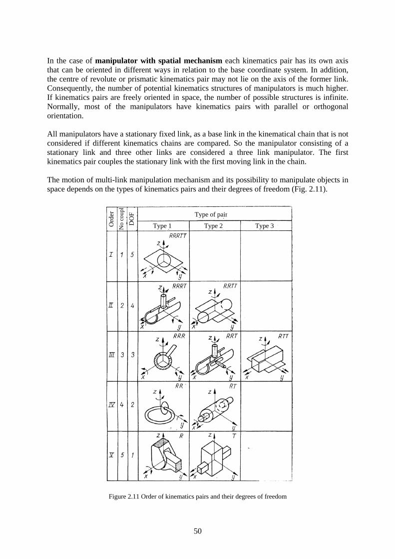
In the case of manipulator with spatial mechanism each kinematics pair has its own axis that can be oriented in different ways in relation to the base coordinate system. In addition, the centre of revolute or prismatic kinematics pair may not lie on the axis of the former link. Consequently, the number of potential kinematics structures of manipulators is much higher. If kinematics pairs are freely oriented in space, the number of possible structures is infinite. Normally, most of the manipulators have kinematics pairs with parallel or orthogonal orientation. All manipulators have a stationary fixed link, as a base link in the kinematical chain that is not considered if different kinematics chains are compared. So the manipulator consisting of a stationary link and three other links are considered a three link manipulator. The first kinematics pair couples the stationary link with the first moving link in the chain. The motion of multi-link manipulation mechanism and its possibility to manipulate objects in space depends on the types of kinematics pairs and their degrees of freedom (Fig. 2.11).

Figure 2.11 Order of kinematics pairs and their degrees of freedom

Type of pair

Type 1 Type 2 Type 3DO

F N

o co

upl

No

coup

lO

rder

O

rder

50

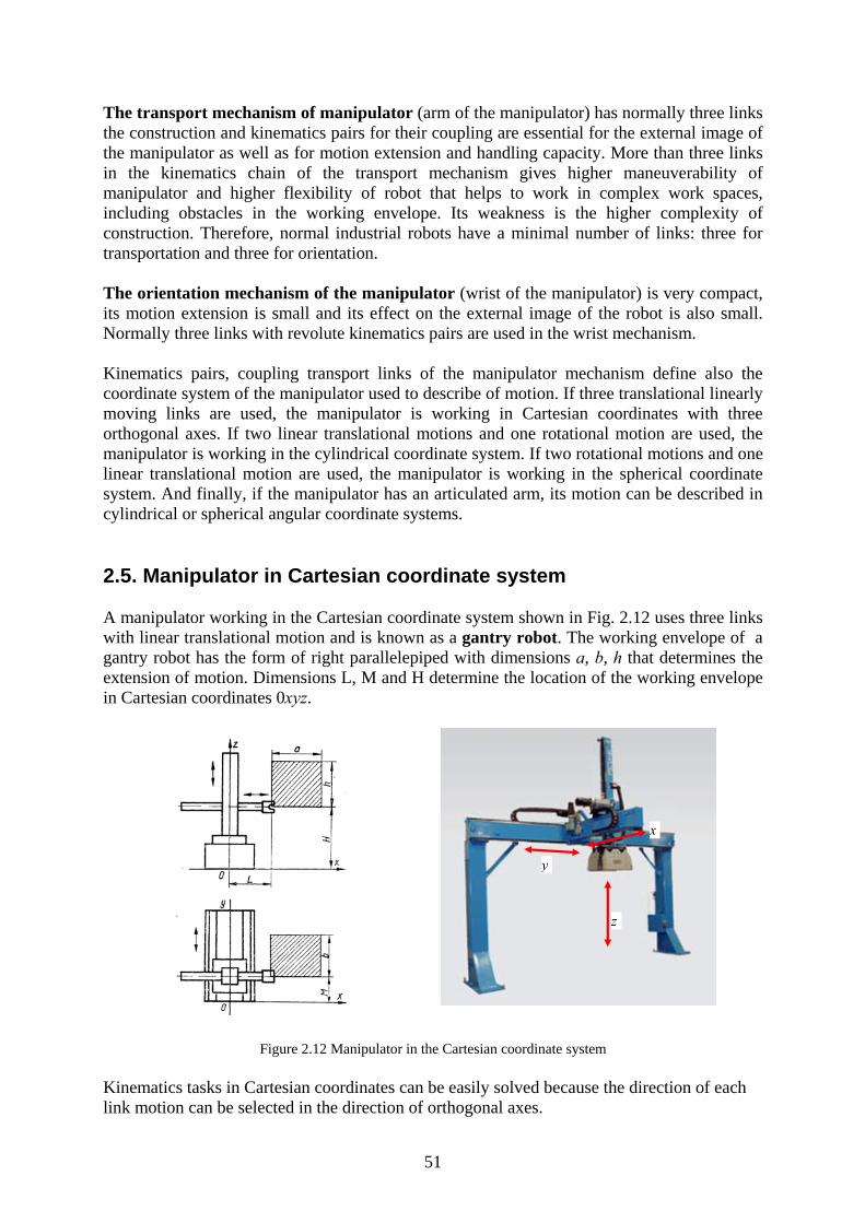
The transport mechanism of manipulator (arm of the manipulator) has normally three links the construction and kinematics pairs for their coupling are essential for the external image of the manipulator as well as for motion extension and handling capacity. More than three links in the kinematics chain of the transport mechanism gives higher maneuverability of manipulator and higher flexibility of robot that helps to work in complex work spaces, including obstacles in the working envelope. Its weakness is the higher complexity of construction. Therefore, normal industrial robots have a minimal number of links: three for transportation and three for orientation. The orientation mechanism of the manipulator (wrist of the manipulator) is very compact, its motion extension is small and its effect on the external image of the robot is also small. Normally three links with revolute kinematics pairs are used in the wrist mechanism. Kinematics pairs, coupling transport links of the manipulator mechanism define also the coordinate system of the manipulator used to describe of motion. If three translational linearly moving links are used, the manipulator is working in Cartesian coordinates with three orthogonal axes. If two linear translational motions and one rotational motion are used, the manipulator is working in the cylindrical coordinate system. If two rotational motions and one linear translational motion are used, the manipulator is working in the spherical coordinate system. And finally, if the manipulator has an articulated arm, its motion can be described in cylindrical or spherical angular coordinate systems. 2.5. Manipulator in Cartesian coordinate system A manipulator working in the Cartesian coordinate system shown in Fig. 2.12 uses three links with linear translational motion and is known as a gantry robot. The working envelope of a gantry robot has the form of right parallelepiped with dimensions a, b, h that determines the extension of motion. Dimensions L, M and H determine the location of the working envelope in Cartesian coordinates 0xyz.

x

z

y

Figure 2.12 Manipulator in the Cartesian coordinate system

Kinematics tasks in Cartesian coordinates can be easily solved because the direction of each link motion can be selected in the direction of orthogonal axes.

51

2.6. Manipulator in cilindrical coordinate system The working envelope of a manipulator in the cylindrical coordinate system is the part of a hollow cylinder. Examples of manipulators in the cylindrical coordinate system are shown in Figs. 2.13 and 2.14. The base or the world coordinate system is bound to the manipulator stationary base. More information about manipulator coordinate systems can be found from website http://prime.jsc.nasa.gov/ROV/types.html

Figure 2.13. Manipulator in the cylindrical coordinate system: a working envelope for vertical axis robot, b working envelope for horizontal axis robot, examples of Versatran, Seiko RT3300 and Fanuc M300 robots

The following is the mathematical description of the manipulator shown in Fig 2.14. Position vector

z

y

x

A

ppp

P =r

, (2.46)

where

52

( )(

hZp

RbpRbp

z

cy

cx

+=

++= )++=αααααα

sinsincoscos

(2.47)

A

z2

z0

z1

x2

y2

y0

x0

y1

x1

Z

R

α

PA

αc

α

h

b

y3

z3

x3

Figure 2.14 Calculation scheme for the manipulator working in the cylindrical coordinate system

Equations describing geometrical components of the position vector can be used to solve manipulator kinematics tasks. This method is named the geometrical method of solution of manipulator kinematics tasks. Complexity of the equations and their solving procedure depends on the configuration of the manipulator and used coordinate system. Principally, these equations can be used for direct as well as for indirect kinematics tasks. Difficulties can exist if the equations are transcendental. In this case there are no general solutions but only numerical values for solution exist. Rotation matrixes

1000cossin0sincos

01 αα

αα −=R

1000cossin0sincos

12 cc

cc

R αααα −

= (2.48)

Transformation matrixes

100000100100

001

23

R

T

−

=

1000100

00cossin00sincos

01 ZT

αααα −

=

1000100

00cossin0sincos

12 h

b

T cc

cc

αααα −

= (2.49)

Articulated arm manipulator working in cylindrical coordinates (i.e. SCARA-type manipulator) has also a hollow cylinder form working envelope. It must be added that the cylinder axis may be vertical or horizontal. That kind of robots are shown in Fig. 2.15. The kinematics of the SCARA-type robot is shown in Fig. 2.16.

53

The motion of the horizontal articulated arm robot is described by simple equations and a simple solution exists for direct as well as for indirect kinematics tasks. The position of manipulator’s tool or gripper is defined by point A, location of which may be determined in the Cartesian coordinates 0xyz or in cylindrical coordinates 0α1α z. 2

Figure 2.15 Articulated arm robots working in the cylindrical coordinate system: with the horizontal axis and vertical axis

A

z0

z1

y0

x0

Z

α1 PA

b

y3

z3

x3

x1

y1

α2

z2

x2

y2

x

y

α1

L1

α2

L2

xA

yA

A

Figure 2.16 Calculation scheme for the articulated arm robot working in the cylindrical coordinate system

The manipulator direct kinematics task can be solved using the following system of equations:

( )(

aa

a

a

zzLLyLLx

=++=++=

21211

21211

sinsincoscos

ααα )ααα

(2.50)

Using equations (2.50) it is possible also to solve the inverse kinematics task of the manipulator, but it must be considered that the calculation of angles α , and α1 2 may be complicated. Because of this the other solution based on the geometrical construction in Fig. 2.17 can be used to solve the inverse kinematics task of the manipulator.

54

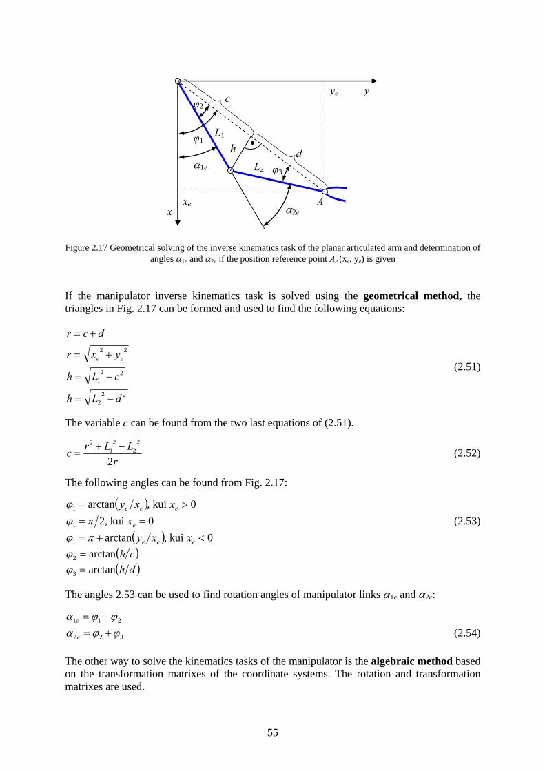
x

y

α1e

L1

α2e

L2

xe

ye

A

c

dhφ1

φ2

φ3

Figure 2.17 Geometrical solving of the inverse kinematics task of the planar articulated arm and determination of

angles α if the position reference point A and α (x , y ) is given 1e 2e e e e

If the manipulator inverse kinematics task is solved using the geometrical method, the triangles in Fig. 2.17 can be formed and used to find the following equations:

222

221

22

dLh

cLh

yxr

dcr

ee

−=

−=

+=

+=

(2.51)

The variable c can be found from the two last equations of (2.51).

rLLrc

2

22

21

2 −+= (2.52)

The following angles can be found from Fig. 2.17:

( )

( ) 0kui,arctan0kui,2

0kui,arctan

1

1

1

<+===

>=

eee

e

eee

xxyx

xxy

πϕπϕ

ϕ (2.53)

( )charctan2 =ϕ ( )dharctan3 =ϕ

The angles 2.53 can be used to find rotation angles of manipulator links α1e and α2e:

211 ϕϕα −=e

322 ϕϕα +=e (2.54) The other way to solve the kinematics tasks of the manipulator is the algebraic method based on the transformation matrixes of the coordinate systems. The rotation and transformation matrixes are used.

55

In the case of the manipulator (Fig. 2.16), coordinate system 3 is rotated by 90º around z-axis of coordinate system 2 and then once 90º around x-axis. Rotation matrixes

1000cossin0sincos

11

1101 αα

αα −=R

1000cossin0sincos

22

2212 αα

αα −=R (2.55)

Transformation matrixes

1000100

00cossin00sincos

11

11

01 hT

αααα −

=

100000100001

100 2

23

r

T =

1000100

00cossin0sincos

22

122

12 b

r

Tαααα −

= (2.56)

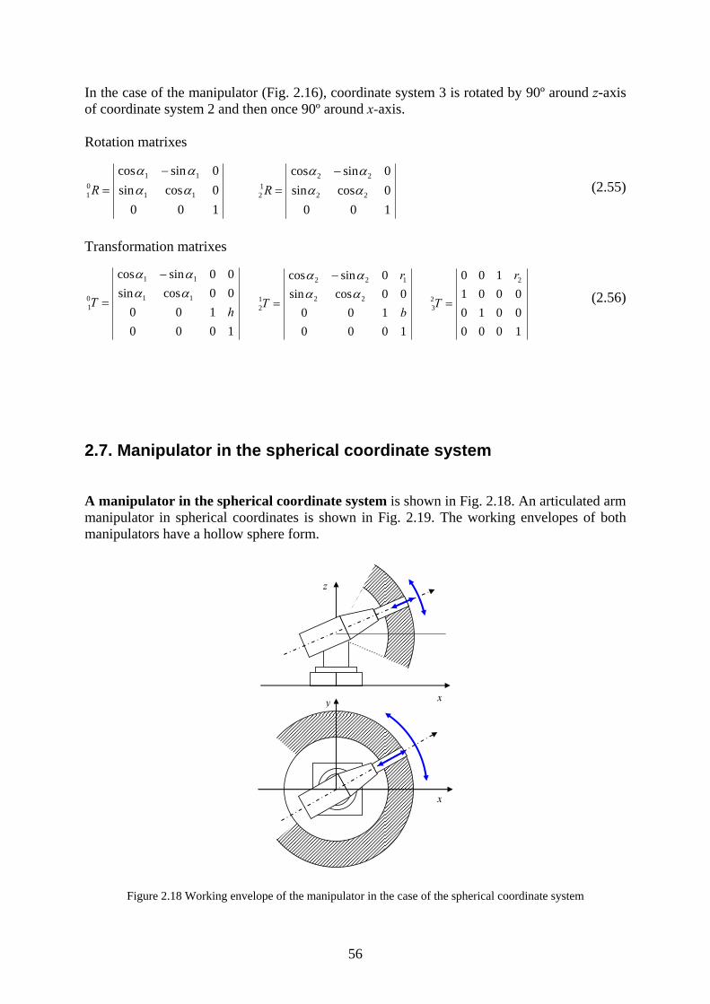
2.7. Manipulator in the spherical coordinate system A manipulator in the spherical coordinate system is shown in Fig. 2.18. An articulated arm manipulator in spherical coordinates is shown in Fig. 2.19. The working envelopes of both manipulators have a hollow sphere form.

y

x

z

x

Figure 2.18 Working envelope of the manipulator in the case of the spherical coordinate system

56

J5 axis

J3 axis

J2 axis

J6 axis

J4 axis

J1 axis Base

Shoulder

Elbow

Wrist

ÕlavarsMechanical interface for connection of gripper

Wrist

Forearm

Trunk

Upper arm

Shoulder

Figure 2.19 Articulated arm robots working in the spherical coordinates: a 6 DOF manipulator of Mitsubishi Co and b PUMA 560 manipulator of Unimation Co

A

z0

z2

y0

x0

h

α3

PA

r1x2y2

α1 x3

r2

b

z3

y3

y4

z4

x4

aα2 z1

y1x1

Figure 2.20 Calculation scheme for the articulated arm manipulator working in the spherical angular coordinates Coordinates of the manipulator second link (Fig. 2.20) are rotated 90º around z coordinate of the first link, rotated 90º around the x coordinate and then rotated by α around z-axis. 2 Transformation matrixes of coordinate systems:

1000010000cossin00sincos

11

11

01

αααα −

=T

10001cossin

00sincos000

22

2212 h

a

Tαααα −

=

57

1000100

00cossin0sincos

11

111

23 b

r

T−

−

=αααα

100000010010

100 2

34 −

=

r

T (2.57)

Rotation matrix of the component of the transformation matrix can be found as the product of two rotation matrixes. The first describes the right angle rotation around z and x axis and the second describes the rotation by α

T12

around z axis. 2

1cossin0sincos000

1000cossin0sincos

010001100

22

2222

2212

αααααα

αα−=

−×=R (2.58)

Pr

0Position vector in coordinates 0 can be found as the product of transformation matrix and vector

T04

Pr

4

PTPrr

404

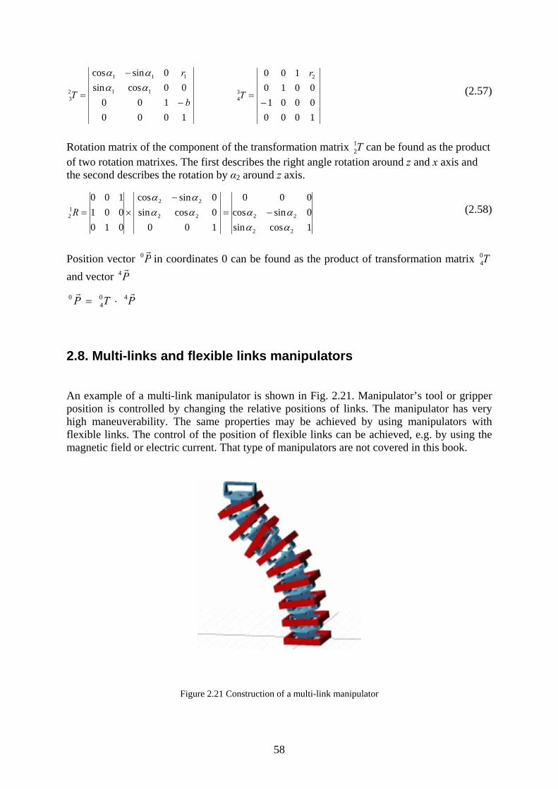
0 ⋅= 2.8. Multi-links and flexible links manipulators An example of a multi-link manipulator is shown in Fig. 2.21. Manipulator’s tool or gripper position is controlled by changing the relative positions of links. The manipulator has very high maneuverability. The same properties may be achieved by using manipulators with flexible links. The control of the position of flexible links can be achieved, e.g. by using the magnetic field or electric current. That type of manipulators are not covered in this book.

Figure 2.21 Construction of a multi-link manipulator

58

2.9. Parallel kinematics of manipulators Traditionally manipulators have a series configuration of links. In this case the drives of moving links are also located on the link chain and normally they are placed on previous links in relation to the moved link. It means that weight of each drive is a payload for the previous drive. In the case of wrist it is very difficult to locate massive drives near the gripper or tool. The solution is the location of all wrist drives on the last transportation link of the manipulator and use of complex multi-coordinate manipulator transmission gears (manipulator transmission mechanisms). With the help of these transmission mechanisms drives can be removed farther from the gripper or tool, but the weight of drives is still a problem in terms of better dynamical properties of a robot. A new direction in the development of industrial robotics is to use manipulators with parallel kinematics. Because these robots have totally different external image of the body of a traditional robot on several columns (legs), they are named as Trepod or Hexapod (Fig. 2.22) or (Figs. 2.23 and 2.24). The same type of a robot is also the ABB robot FlexPicker. Additional information about manipulators with parallel kinematics is available on websites: http://www.parallemic.org/Terminology/General.html http://www.parallemic.org/SiteMap.html Advantages of manipulators having parallel kinematics structure:

3-6 motors driving small weight links and one gripper or tool of a manipulator. Due to small weight and mass and little moment of inertia the robot has very high dynamic properties.

positioning errors of links cannot be summed higher rigidity (mechanical accuracy) no moving connection cables higher accuracy and repeatability higher reliability

Robot image from website: http://www.parallemic.org/Reviews/Review002.html

Figure 2.22 Three-leg manipulator with parallel kinematics in the suspended pose

59

Spherical joint S

Spherical joint S Fixed base

Moving platform

Translational- pair P

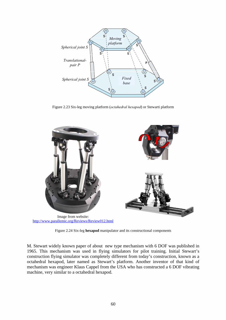
Figure 2.23 Six-leg moving platform (octahedral hexapod) or Stewarti platform

Image from website: http://www.parallemic.org/Reviews/Review012.html

Figure 2.24 Six-leg hexapod manipulator and its constructional components

M. Stewart widely known paper of about new type mechanism with 6 DOF was published in 1965. This mechanism was used in flying simulators for pilot training. Initial Stewart’s construction flying simulator was completely different from today’s construction, known as a octahedral hexapod, later named as Stewart’s platform. Another inventor of that kind of mechanism was engineer Klaus Cappel from the USA who has constructed a 6 DOF vibrating machine, very similar to a octahedral hexapod.

60

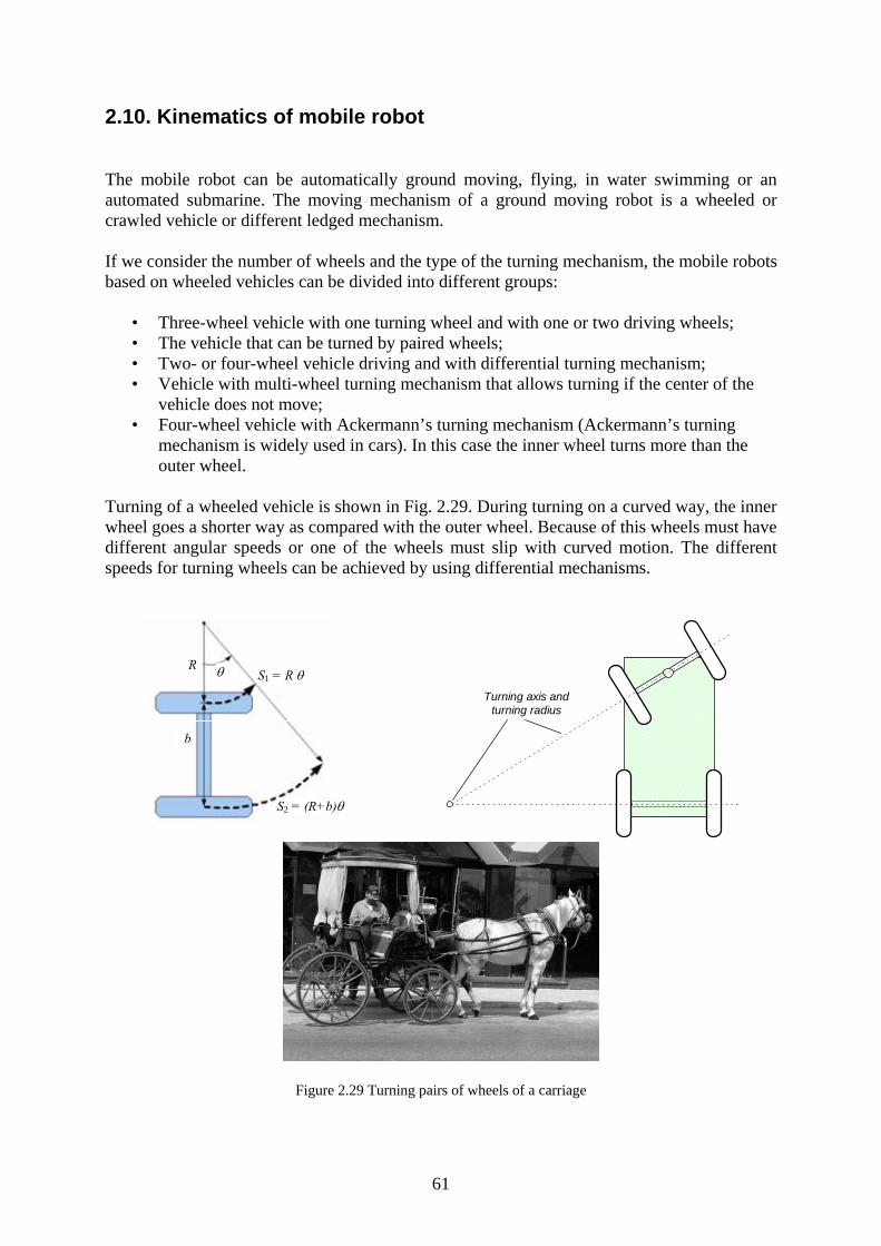
2.10. Kinematics of mobile robot The mobile robot can be automatically ground moving, flying, in water swimming or an automated submarine. The moving mechanism of a ground moving robot is a wheeled or crawled vehicle or different ledged mechanism. If we consider the number of wheels and the type of the turning mechanism, the mobile robots based on wheeled vehicles can be divided into different groups:

• Three-wheel vehicle with one turning wheel and with one or two driving wheels; • The vehicle that can be turned by paired wheels; • Two- or four-wheel vehicle driving and with differential turning mechanism; • Vehicle with multi-wheel turning mechanism that allows turning if the center of the

vehicle does not move; • Four-wheel vehicle with Ackermann’s turning mechanism (Ackermann’s turning

mechanism is widely used in cars). In this case the inner wheel turns more than the outer wheel.

Turning of a wheeled vehicle is shown in Fig. 2.29. During turning on a curved way, the inner wheel goes a shorter way as compared with the outer wheel. Because of this wheels must have different angular speeds or one of the wheels must slip with curved motion. The different speeds for turning wheels can be achieved by using differential mechanisms.

Turning axis and turning radius

b

S2 = (R+b)θ

S1 = R θ θ R

Figure 2.29 Turning pairs of wheels of a carriage

61

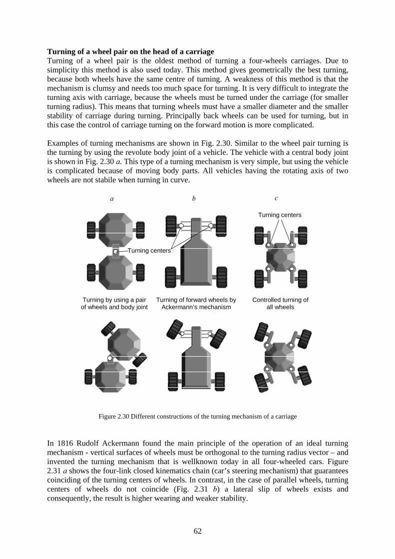
Turning of a wheel pair on the head of a carriage Turning of a wheel pair is the oldest method of turning a four-wheels carriages. Due to simplicity this method is also used today. This method gives geometrically the best turning, because both wheels have the same centre of turning. A weakness of this method is that the mechanism is clumsy and needs too much space for turning. It is very difficult to integrate the turning axis with carriage, because the wheels must be turned under the carriage (for smaller turning radius). This means that turning wheels must have a smaller diameter and the smaller stability of carriage during turning. Principally back wheels can be used for turning, but in this case the control of carriage turning on the forward motion is more complicated. Examples of turning mechanisms are shown in Fig. 2.30. Similar to the wheel pair turning is the turning by using the revolute body joint of a vehicle. The vehicle with a central body joint is shown in Fig. 2.30 a. This type of a turning mechanism is very simple, but using the vehicle is complicated because of moving body parts. All vehicles having the rotating axis of two wheels are not stabile when turning in curve.

Turning by using a pair of wheels and body joint

Turning of forward wheels by Ackermann’s mechanism

Controlled turning of all wheels

Turning centers

Turning centers

a b c

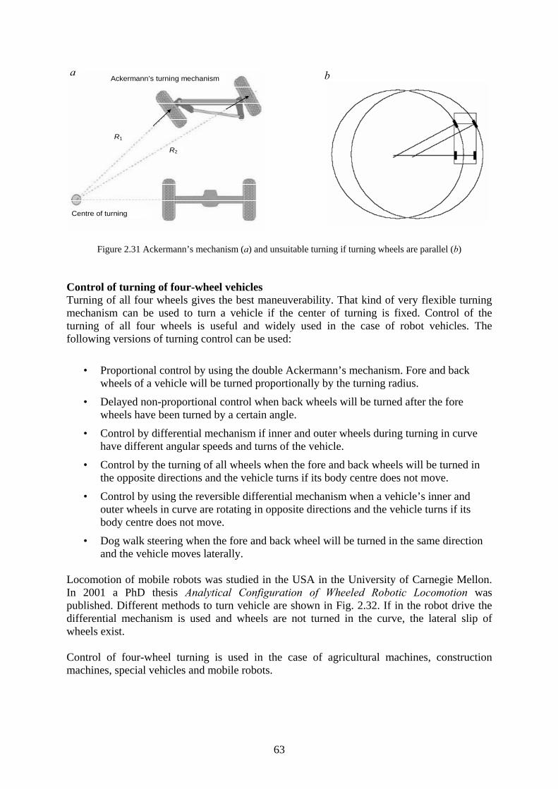
Figure 2.30 Different constructions of the turning mechanism of a carriage In 1816 Rudolf Ackermann found the main principle of the operation of an ideal turning mechanism - vertical surfaces of wheels must be orthogonal to the turning radius vector – and invented the turning mechanism that is wellknown today in all four-wheeled cars. Figure 2.31 a shows the four-link closed kinematics chain (car’s steering mechanism) that guarantees coinciding of the turning centers of wheels. In contrast, in the case of parallel wheels, turning centers of wheels do not coincide (Fig. 2.31 b) a lateral slip of wheels exists and consequently, the result is higher wearing and weaker stability.

62

Centre of turning

Ackermann’s turning mechanism

R1

R2

a b

Figure 2.31 Ackermann’s mechanism (a) and unsuitable turning if turning wheels are parallel (b) Control of turning of four-wheel vehicles Turning of all four wheels gives the best maneuverability. That kind of very flexible turning mechanism can be used to turn a vehicle if the center of turning is fixed. Control of the turning of all four wheels is useful and widely used in the case of robot vehicles. The following versions of turning control can be used:

• Proportional control by using the double Ackermann’s mechanism. Fore and back wheels of a vehicle will be turned proportionally by the turning radius.

• Delayed non-proportional control when back wheels will be turned after the fore wheels have been turned by a certain angle.

• Control by differential mechanism if inner and outer wheels during turning in curve have different angular speeds and turns of the vehicle.

• Control by the turning of all wheels when the fore and back wheels will be turned in the opposite directions and the vehicle turns if its body centre does not move.

• Control by using the reversible differential mechanism when a vehicle’s inner and outer wheels in curve are rotating in opposite directions and the vehicle turns if its body centre does not move.

• Dog walk steering when the fore and back wheel will be turned in the same direction and the vehicle moves laterally.

Locomotion of mobile robots was studied in the USA in the University of Carnegie Mellon. In 2001 a PhD thesis Analytical Configuration of Wheeled Robotic Locomotion was published. Different methods to turn vehicle are shown in Fig. 2.32. If in the robot drive the differential mechanism is used and wheels are not turned in the curve, the lateral slip of wheels exist. Control of four-wheel turning is used in the case of agricultural machines, construction machines, special vehicles and mobile robots.

63

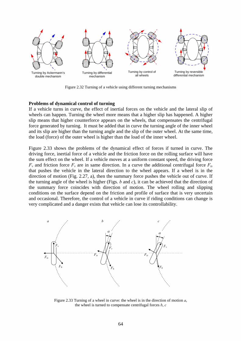
Turning by control ofall wheels

Turning by reversible differential mechanism

Turning by differential mechanism

Turning by Ackermann’s double mechanism

Figure 2.32 Turning of a vehicle using different turning mechanisms

Problems of dynamical control of turning If a vehicle turns in curve, the effect of inertial forces on the vehicle and the lateral slip of wheels can happen. Turning the wheel more means that a higher slip has happened. A higher slip means that higher counterforce appears on the wheels, that compensates the centrifugal force generated by turning. It must be added that in curve the turning angle of the inner wheel and its slip are higher than the turning angle and the slip of the outer wheel. At the same time, the load (force) of the outer wheel is higher than the load of the inner wheel. Figure 2.33 shows the problems of the dynamical effect of forces if turned in curve. The driving force, inertial force of a vehicle and the friction force on the rolling surface will have the sum effect on the wheel. If a vehicle moves at a uniform constant speed, the driving force Fv and friction force Fv are in same direction. In a curve the additional centrifugal force Fts that pushes the vehicle in the lateral direction to the wheel appears. If a wheel is in the direction of motion (Fig. 2.27, a), then the summary force pushes the vehicle out of curve. If the turning angle of the wheel is higher (Figs. b and c), it can be achieved that the direction of the summary force coincides with direction of motion. The wheel rolling and slipping conditions on the surface depend on the friction and profile of surface that is very uncertain and occasional. Therefore, the control of a vehicle in curve if riding conditions can change is very complicated and a danger exists that vehicle can lose its controllability.

a b

Fh

Fv

Fts

Fh

Fv

Fts

c

Fh

Fv

Fts

α α

Figure 2.33 Turning of a wheel in curve: the wheel is in the direction of motion a, the wheel is turned to compensate centrifugal forces b, c

64

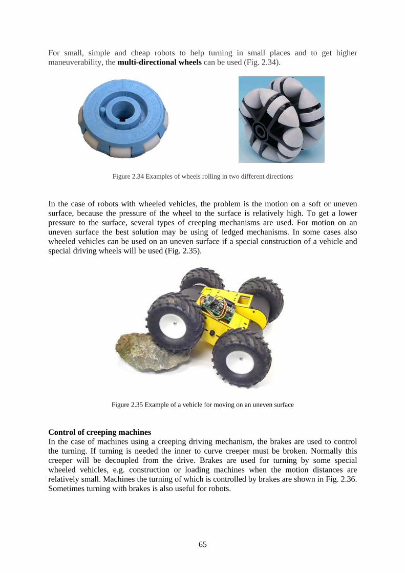
For small, simple and cheap robots to help turning in small places and to get higher maneuverability, the multi-directional wheels can be used (Fig. 2.34).

Figure 2.34 Examples of wheels rolling in two different directions In the case of robots with wheeled vehicles, the problem is the motion on a soft or uneven surface, because the pressure of the wheel to the surface is relatively high. To get a lower pressure to the surface, several types of creeping mechanisms are used. For motion on an uneven surface the best solution may be using of ledged mechanisms. In some cases also wheeled vehicles can be used on an uneven surface if a special construction of a vehicle and special driving wheels will be used (Fig. 2.35).

Figure 2.35 Example of a vehicle for moving on an uneven surface Control of creeping machines In the case of machines using a creeping driving mechanism, the brakes are used to control the turning. If turning is needed the inner to curve creeper must be broken. Normally this creeper will be decoupled from the drive. Brakes are used for turning by some special wheeled vehicles, e.g. construction or loading machines when the motion distances are relatively small. Machines the turning of which is controlled by brakes are shown in Fig. 2.36. Sometimes turning with brakes is also useful for robots.

65

Figure 2.36 Machines using a crawling driving mechanism and brakes for turning (Photos of Uwe Berg from Internet)

Walking robots or ledged robots Walking or ledged robots are copied from nature. Depending on the number of legs, walking robots can be divided as follows:

• One-leg robots • Two-leg robots • Three-leg robots • Four-leg robots • Six-leg robots • Eight-leg robots • Multi-leg robots (hundred-leg robots)

If one- or two-leg robots are used, an additional problem of keeping balance appears. Generally to control balance of a robot, dynamic feedback from acceleration sensors is needed. Three-leg robots are used seldom because the same problem to keep balance if the third leg is moved exist. Mainly three-leg robots are useful for climbing. Phases of motion of a two-leg walking mechanism are shown in Fig. 2.37.

1 432

II I II I III II I

Figure 2.37 Phases of motion of a two-leg walking mechanism Walking starts if the weight of a body is transferred to the stretched leg (II) and free leg movement in the direction of motion. In the second phase of walking, leg (I) is in its final forward position. In the third phase of walking, this leg will be put to ground. In the fourth phase of walking, the weight of a body will be transferred to leg (I). These phases will be repeated cyclically and the free leg (II) will be moved in the direction of walking motion.

66

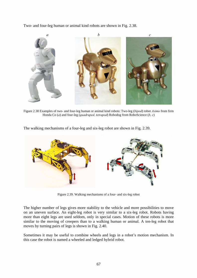
Two- and four-leg human or animal kind robots are shown in Fig. 2.38.

a b c

Figure 2.38 Examples of two- and four-leg human or animal kind robots: Two-leg (bipod) robot Asimo from firm

Honda Co (a) and four-leg (quadruped, tetrapod) Robodog from RoboScience (b, c) The walking mechanisms of a four-leg and six-leg robot are shown in Fig. 2.39.

Figure 2.39. Walking mechanisms of a four- and six-leg robot The higher number of legs gives more stability to the vehicle and more possibilities to move on an uneven surface. An eight-leg robot is very similar to a six-leg robot. Robots having more than eight legs are used seldom, only in special cases. Motion of these robots is more similar to the moving of creepers than to a walking human or animal. A ten-leg robot that moves by turning pairs of legs is shown in Fig. 2.40. Sometimes it may be useful to combine wheels and legs in a robot’s motion mechanism. In this case the robot is named a wheeled and ledged hybrid robot.

67

Figure 2.40 Ten-leg robot that moves by the turning pairs of legs Hybrid vehicles using legs and wheels Legs give more possibilities to overcome obstacles but wheels have a simpler construction and the motion is more efficient. Examples of hybrid robots are shown in Fig. 2.41.

Figure 2.41 Hybrid vehicles using legs and wheels

Three-leg climbing robot. The kinematics of a three-leg climbing robot is shown in Fig. 2.42. Two legs of the robot are used for holding and the third leg moves to the new place of holding. Legs move using the chain of leg links coupled by the revolute kinematics pairs.

Holding leg 1 Holding leg 2

Holding place 3 Free leg 3

Kinematics chain

Pelvis of legs

Figure 2.42 Climbing mechanism

68