Subsea Production System for Gas Field Offshore Brazil - 1 - Federal University of Rio de Janeiro Naval Architecture and Ocean Engineering Department International Student Offshore Design Competition 2005 Subsea Production System for Gas Field Offshore Brazil Tiago Pace Estefen Daniel Santos Werneck Diogo do Amaral Macedo Amante João Paulo Carrijo Jorge Leandro Cerqueira Trovoado Faculty Advisor: Prof. Segen F. Estefen

Welcome message from author
This document is posted to help you gain knowledge. Please leave a comment to let me know what you think about it! Share it to your friends and learn new things together.
Transcript
Subsea Production System for Gas Field Offshore Brazil
- 1 -
Federal University of Rio de Janeiro Naval Architecture and Ocean Engineering Department
International Student Offshore Design Competition 2005
Subsea Production System for Gas Field Offshore Brazil
Tiago Pace Estefen Daniel Santos Werneck
Diogo do Amaral Macedo Amante João Paulo Carrijo Jorge
Leandro Cerqueira Trovoado
Faculty Advisor: Prof. Segen F. Estefen
Subsea Production System for Gas Field Offshore Brazil
- 2 -
CONTENTS LIST OF FIGURES 05 LIST OF TABLE 07 EXECUTIVE SUMMARY 08 ACKNOWLEDGEMENTS 14 1. INTRODUCTION 15 1.1 Team Organization 16 2. SYSTEM DESIGN 18 2.1. Sub-systems, Equipments and Components 18 2.1.1. Pipes 18 2.1.2. Umbilical Cable 18 2.1.3. Control System 19 2.1.4. Wet Christmas Tree (X-Tree) 19 2.1.5. Manifold 19 2.1.6. Pipe Line End Manifold - PLEM 20 2.1.7. Pipe Line End Termination – PLET 20 2.1.8. Jumper 20
2.2. Layout of the System 21 2.2.1. Semi-submersible 22 2.2.2. Jacket 23 2.2.3. Subsea to Beach 24 3. SUBSEA PROCESSING 26 3.1. Hydrates 26 3.2. Types of Thermal Insulation 27 3.2.1. Thermal Insulation Adopted 27 3.3. Gas State Properties 28 3.4. Temperature and Pressure Profile Determination 29 3.4.1. Temperature Profile 29 3.4.2. Pressure Profile 31 3.4.3. Scenario 1: Semi-Submersible 31 3.4.4. Scenario 2: Jacket 33 3.4.5. Scenario 3: Subsea to Beach 36 3.5.Transient Regime 39 3.6. Mono Ethylene Glycol 40 3.6.1. Recycle 41 3.6.2. MEG Calculation 43 3.7. Concluding Remarks 43 4. FLOWLINES AND RISERS 44 4.1. Design of Flowlines and Rigid Risers 44
4.1.1. Local Buckling Due to Longitudinal Strain and External Overpressure 45 4.1.2. Propagation Buckling 47 4.1.3. Local Buckling Due to Bending Moment, Effective Axial Force and Internal Overpressure 47
4.1.4. Material Properties 49 4.1.5. Results 49
4.2 Riser Analyzes Considering Top Motions 50 4.2.1. Semi-submersible Platform Gas - Production Riser 50
4.2.1.1. System Configuration 50 4.2.1.2. Relevant Parameters 51 4.2.1.3. Soil Data 51 4.2.1.4. Structural Properties 51 4.2.1.5. Environmental Data 52 4.2.1.6. Extreme Offset 52
Subsea Production System for Gas Field Offshore Brazil
- 3 -
4.2.1.7. Numerical Model 52 4.2.1.8. Global Analysis Results – Import Riser 53
4.2.1.9. Considerations about the Results for Import Flexible Risers 55 4.2.2. Semi-Submersible Platform Gas Export Riser 55
4.2.2.1. System Configuration 56 4.2.2.2. Relevant Analysis Parameters 57 4.2.2.3. Structural Properties 57 4.2.2.4. Numerical Model 58 4.2.2.5. Global Analysis Results – Export Riser 60 4.2.2.6. Considerations about the Results for Export Hybrid Risers 62
4.3. Pipe installation 62 4.3.1. S-Lay Method 63 4.3.2. J-Lay method 63 4.3.3. Reel Method 63 4.3.4. Definition of the Installation Method 64
4.4 Pipe Maintenance - Inspection and Cleaning 64 4.4.1 Geometric Pig 65
4.4.2 Corrosion Pig 66 5. SUBSEA SYSTEM DESIGN 67 5.1. Wet Christmas Tree (X-Tree) 67
5.1.2. X-Tree installation Method 67 5.1.3. X-Tree Arrangement and Operation 68 5.1.4. Description of selected X-Tree Components 70
5.1.4.1. Choke 70 5.1.4.2. Base for the Flowlines 70 5.1.4.3. Tubing Hanger 70 5.1.4.4. Vertical Connection Module (VCM) 70 5.1.5.5. Tree Cap 70
5.2. Manifold 70 5.2.1. Manifold Installation 71 5.2.2. Manifold Arrangement and Operation 71
5.3. PLEM 73 5.3.1. PLEM Definition 73 5.3.2. PLEM Arrangement, Operability and Installation 73
5.4. PLET 74 5.4.1. PLET Definition 74 5.4.2. PLET Arrangement, Operation and Installation 74
5.5. Control Systems 74 5.5.1. Hydraulic Direct 74 5.5.2. Multiplex Electro Hydraulic 75
5.6 Equipment General Arrangement 75 5.7. Subsea Compression and Separation 77 5.7.1. Subsea Separation 77 5.7.2. Subsea Compression 77 5.7.3. Process Description 77 6. RISK ASSESSMENT 79 6.1. Scenario 1: Semi-Submersible 79 6.2. Scenario 2: Jacket 80 6.3. Scenario 3: Subsea to Beach 82 6.4. Concluding Remarks 84 6.4.1. Total Production Loss 84 6.4.2. Partial Production Loss 85 6.4.3. The Best Scenario 85 7. COSTS 86 7.1. Net Present Value (NPV) 86
Subsea Production System for Gas Field Offshore Brazil
- 4 -
7.2. Master Schedule 86 7.3. MEG/Insulation Analysis 90 7.4. Cost Analysis for the Three Scenarios 91 7.5. Concluding Remarks 97 8. CONCLUSIONS 98 9. REFERENCES 100 APPENDIX A 101 APPENDIX B 109 APPENDIX C 111
Subsea Production System for Gas Field Offshore Brazil
- 5 -
List of Figures Figure 1.1: Gantt Chart for UFRJ Team 17 Figure 2.1: Rigid and Flexible Pipes 18 Figure 2.2: Umbilical Cable 19 Figure 2.3: Pipe Line End Manifold 20 Figure 2.4: Pipe Line End Termination 20 Figure 2.5: Jumper 21 Figure 2.6: Wells Layout for Tucunaré Gas Field 22 Figure 2.7: Semi-Submersible Platform Arrangement 23 Figure 2.8: Jacket Platform Arrangement 24 Figure 2.9: Subsea to Beach Arrangement 25 Figure 3.1: Hydrate Plug Removed from a Gas Pipeline 26 Figure 3.2: Phase Diagram Showing the Conditions under which Hydrates will Form 28 Figure 3.3: Temperature Profile with Flow Rate of 10 million m3 / day, Scenario 1: Semi-Submersible 31 Figure 3.4: Basic Diagram of a Collection System, Scenario 1: Semi-Submersible 32 Figure 3.5: Pressure Profile with Flow Rate of 10 million m3 / day, for Scenario 1: Semi-Submersible 32 Figure 3.6: Thermodynamic State (pressure, temperature) in the Phase Equilibrium Diagram of Gas Hydrate, Scenario 1: Semi-Submersible 33 Figure 3.7: Temperature Profile with Flow Rate of 10 million m3 / day, Scenario 2: Jacket 34 Figure 3.8: Basic Diagram of a Collection System, Scenario 2: Jacket 34 Figure 3.9: Pressure Profile for Scenario 2 with Flow rate of 10 million m3 / day, Scenario 2: Jacket 35 Figure 3.10: Thermodynamic State (pressure, temperature) in the Phase Equilibrium Diagram of Gas Hydrate, Scenario 2: Jackets 35 Figure 3.11: Temperature Profile with Flow Rate of 10 million m3 / day, Scenario 3: Subsea to Beach 36 Figure 3.12: Basic Diagram of a Collection System, Scenario 3: Subsea to Beach 37 Figure 3.13: Pressure Profile with Flow Rate of 10 million m3 / day, Scenario 3: Subsea to Beach 37 Figure 3.14: Thermodynamic State (pressure, temperature) in the Phase Equilibrium Diagram of Gas Hydrate, scenario 3: Subsea to Beach 38 Figure 3.15: OLGA Results for Scenario 3 with Flow Rate of 20 million m3/day 38 Figure 3.16: Temperature and Pressure Profile for Scenario 3 with Flow Rate of 20 million m3/day. 39 Figure 3.17: OLGA Results for Transient Analysis at Production Shut Down 39 Figure 3.18: Time Required for Pressure Drop, Scenario 3. 40 Figure 3.19: Full Reclamation MEG Process 41 Figure 3.20: Photo of MEG Process 42 Figure 3.21: MEG Concentration 43 Figure 4.1: System Configuration 50 Figure 4.2: Numerical Model 53 Figure 4.3: Offset Near and Far 54 Figure 4.4: Single Line Offset Riser 56 Figure 4.5: System Configuration 57 Figure 4.6: Numerical Model 59 Figure 4.7: Offset Near and Far 60 Figure 4.8: Von Mises Stresses Acting on Rigid Riser 61 Figure 4.9: Tensile Forces Acting on the Rigid Riser 61 Figure 4.10: Tensile Forces Acting on the Flexible Riser 61 Figure 4.11: S-Lay Method 63 Figure 4.12: J-Lay Method 63 Figure 4.13: Reel Method 64
Subsea Production System for Gas Field Offshore Brazil
- 6 -
Figure 4.14: PIG Prototype 65 Figure 4.15: Geometrical Pig 66 Figure 4.16: Corrosion Pig 66 Figure 5.1: Connection with One VCM 67 Figure 5.2: Vertical X-Tree 68 Figure 5.3: Schematic Representation of X-Tree GLL/DLL 69 Figure 5.4: Manifold Submarine for 4 wells 72 Figure 5.5: Manifold Recoverable Module 73 Figure 5.6: PLEM Arrangement 73 Figure 5.7: PLET Arrangement 74 Figure 5.8: Equipment General Arrangement 76 Figure 6.1: Fault Tree for the Semi-submersible Scenario 80 Figure 6.2: Fault Tree for Jacket Scenario 82 Figure 6.3: Fault Tree for Subsea to Beach Scenario 84 Figure 7.1: Semi-Submersible Master Schedule 87 Figure 7.2: Jacket Master Schedule 88 Figure 7.3: Subsea to Beach Master Schedule 89 Figure 7.4: Semi-Submersible Probability NPV Analysis 95 Figure 7.5: Jacket Probability NPV Analysis 96 Figure 7.6: Subsea to Beach Probability NPV Analysis 96
Subsea Production System for Gas Field Offshore Brazil
- 7 -
List of Tables Table 1.1: Team Assignments 16 Table 4.1: Safety Class Resistance Factor 45 Table 4.2: Pressure Load Effect Factor 45 Table 4.3: Fabrication Factor 46 Table 4.4: Load Effect Factors and Load Combinations 48 Table 4.5: Semi-submersible Platform 49 Table 4.6: Jacket Platform 49 Table 4.7: Subsea to Beach 49 Table 4.8: Data for Static and Dynamic Analyzes 51 Table 4.9: Soil Data 51 Table 4.10: Flexible pipe Data 51 Table 4.11: Flexjoint Data 52 Table 4.12: Model Mesh 53 Table 4.13: Results for Centenary Wave Combined with Decenary Current 54 Table 4.14: Results for Decenary Wave with Centenary Current 54 Table 4.15: Ratios Between Obtained Results and Limitations for CW/DC 55 Table 4.16: Ratios Between Obtained Results and Limitations for DW/CC 55 Table 4.17: Data for Static and Dynamic Analyzes 57 Table 4.18: Rigid Pipe Data 57 Table 4.19: Flexible Pipe Data 58 Table 4.20: Buoy Data 58 Table 4.21: Flexjoint data 58 Table 4.22: Model Mesh 59 Table 4.23: Curvature Radius 62 Table 7.1: MEG/Insulation Analysis for Scenario 2 90 Table 7.2: MEG/Insulation Analysis for Scenario 3 91 Table 7.3: Loan Data 92 Table 7.4: Semi-Submersible Cost Analysis 92 Table 7.5: Jacket Platform Cost Analysis 93 Table 7.6: Subsea to Beach Cost Analys 94
- 8 -
EXECUTIVE SUMMARY
SUBSEA PRODUCTION SYSTEM FOR GAS FIELD OFFSHORE BRAZIL
The increase of natural gas in the energy matrix all over the world has posed a strong
demand on offshore exploration and production. Although some new concepts for floating gas
storage have been proposed, options associated with subsea production system and pipeline
export to shore should be better investigated in order to improve performance for the field
proven concepts and to propose innovative unmanned subsea design.
Subsea production systems for gas field offshore Brazil are studied. The project consists
of a layout for submarine production of a gas condensate field called Tucunaré supposed to
enter in operation in four years time. The field is located at a distance of 160 km from the
Brazilian coast at a water depth of 500 m. Water depths decrease reaching 180 m at 140 km
from the coast and then progressively up to the beach. Reservoir data indicate pressure of 530
bar and average temperature of 140 oC. Production is based on eight subsea wells with initial
flow rate of 20 million m3 per day of gas and 2,000 m3 per day of condensate.
Three different options of subsea production systems are studied:
• Scenario 1: Semi-submersible distant 160 km from the coast at water depth of 500 m;
• Scenario 2: Jacket platform distant 140 km from the coast at water depth of 180 m;
• Scenario 3: Subsea to Beach system (without platform).
The methodology used to define and develop the design was based on field proven
technology and new concepts introduced into the design with the support of both computer
simulations and code recommendations for structural integrity, heat transfer and risk
assessment.
The report has been organized in order to cover the 8 declared competencies in specific
chapters, except for Construction, Fabrication and Installation which are treated in chapters 3,
- 9 -
4 and 5 (Subsea Processing, Pipelines and Flowlines; Subsea System Design). Strength and
Structural Design as well as Riser Design are included in chapter 4 (Pipelines and Flowlines).
Risers and pipelines have been design in accordance with DnV recommendations (OS-
F101 and OS-F201). Risk assessment of the designed subsea systems followed the ABS
Guide (Risk Evaluation for the Classification of Marine-Related Facilities).
In this Summary, the main results associated with the 8 declared competencies are
outlined below.
System Design
In order to better present the respective system design, general subsea arrangements were
developed. The semi-submersible was initially considered due to the water depth of 500
meters and its field proven concept, suitable for Brazilian offshore environmental conditions.
The subsea arrangement is constituted of 8 satellite wells with 8” flowline/risers for
production and a hybrid riser configuration (single line offset riser tower - SLOR) for
exportation to shore.
Since the water depth decreases significantly along 20 km into shore direction, reaching
180 meters, the Jacket platform came out as an option. This system presents some advantages
in relation to the Semi-submersible, as the deck motions are not sensitive to waves and
currents. Due to the well distance from the platform, two parallel manifolds capable of
receiving 4 wells each are employed. The manifold headers are connected to Pipe Line End
Manifold (PLEM) by rigid jumpers. Another two similar jumpers connect the PLEM to two
independent Pipe Line End Terminate (PLET). From those equipments, two rigid 18”
flowlines are used as production lines. From the platform, a 22” rigid pipe is responsible for
exportation to shore.
An innovative technological solution represented by an association of subsea production
and direct export to the beach, Subsea to Beach, appeared to be another interesting alternative.
- 10 -
Without a stationary production unit, crew and continuous support vessels are not necessary,
reducing both operational expenditures and human risk. Similar subsea arrangement as
employed for the Jacket scenario is used up to the PLEM. Then, two 22” rigid jumpers are
connected to the PLETs and two pipelines with same diameters export the gas to the onshore
terminal.
Subsea System Design
The subsea system is associated with the overall process and all the equipments involved
in the arrangement. It is designed in a way that safety, environment protection, flow assurance
and reliability are considered for the gas exploitation. Operational and maintenance aspects
were taken into account for the design of the equipments. X-Tree, manifold, PLEM and PLET
were developed to guarantee the safety barriers and operational flexibility in emergency
situations.
Subsea Processing
As gas wells are being developed, hydrate formation in the production system has become
a major concern. Several options are available to manage hydrate formation. Two solutions
were analyzed, thermal insulation and continuous injection of Mono Ethylene Glicol (MEG).
For the three scenarios a series of analyzes have been carried out to determine the
thermodynamic state (pressure and temperature) in the phase equilibrium diagram of gas
hydrate to assure that the flow are out of the hydrate envelope. Analyzing Subsea to Beach,
which represents the most challenging scenario for flow assurance, with flow rate of 10
million m3 per day (by the end of the design life), it has been estimated the U value of 1.05
W/m2 °C for the two export pipelines (22” diameter). For these pipelines, the thermal
insulation proposed was the polypropylene, with solid outer layer of 0.25” and foam inner
layer of 1”. That was enough to insulate the pipeline with an arrival temperature to the
onshore terminal of 14 °C. Finally, using the computer program OLGA for production shut
- 11 -
down and consequent pressure drop, it has been confirmed the insulation adequacy.
Alternatively, continuous injection of MEG was also considered as a tool to prevent the gas
hydrate formation. The necessary quantity of MEG was estimated so that a comparative
economic analysis with the pipe insulation can be made.
Strength and Structural Design / Riser Design
The structural design of rigid pipes (flowlines and rigid pipes) for each of the scenarios
proposed was accomplished using the ultimate limit state, based on criteria related to rigid
pipe local buckling. The DNV recommendations were adopted for the three failure modes,
local buckling due to bending moment, effective axial force and internal overpressure, local
buckling due to longitudinal compressive strain and external overpressure and propagation
buckling. An Excel spread sheet was developed according with DnV criteria and standard
thickness selected as in API Specification for Line Pipe.
The semi-submersible arrangement is the only one subjected to environmental loads
(waves and currents) induced motions. This dynamic behavior affects the riser structural
response, therefore riser structural analyzes under extreme loading were conducted for the
semi-submersible scenario.
Static and dynamic global analyzes for production and export risers were accomplished,
taking into consideration wave and current extreme loading conditions with two return period
combinations, centenary wave with decenary current and decenary wave with centenary
current. Offset directions considered were near, far and transverse. The ANFLEX, especial
purpose program, was used for these riser analyzes. Results for the risers were checked
against the correspondent limit values provided by manufacturer in the cases of flexibles and
verified using API-RP 2RD for steel pipes. Parameters of interest for design verification are
curvature radius, axial forces and Von Mises stresses. The proposed pipes are in compliance
with the both code and manufacturer limitations.
- 12 -
Construction, Fabrication and Installation
Installation methods have been evaluated for flexible and rigid pipes. The reel method is
recommended for the flexible pipes. Due to the large diameter of the rigid riser it is
recommended the installation by the J-lay method. Same approach has been adopted for rigid
flowlines with diameters of 18” and 22”, i.e. installation by J-lay method. All rigid pipes are
API X-65 steel grade and with diameter to thickness ratios of 39 for 18” and 35 for 22”.
X-Tree installation is performed using the guidelineless procedure with vertical
connection module, contributing to optimize the costs due to independent installations of X-
Tree and flowline. Manifolds are installed diverless due to water depth beyond 300 m.
Risk Assessment
Risk assessment for the proposed subsea production systems are performed using fault
tree analyzes to better understand the respective system weakness and to propose safety
improvement measures. Production loss has been assumed as the top failure event.
Total production loss has an associated failure probability substantially smaller than that
for the partial production loss. Therefore, the most reliable scenario should take into
consideration small production losses during the project life cycle. In this case, the satellite
wells with dynamic risers (scenario 1) are the less attractive alternative.
Although equivalent in terms of partial production loss, scenario 3 is more reliable than
scenario 2 for total production loss. Therefore, based on the qualitative risk assessment for
production loss, the scenario 3 can be indicated as the best option for the offshore gas field
considered in this project. The possibility of gas/water subsea separation and subsea gas
compression, before export to onshore terminal, could mean an outstanding advantage for
Subsea to Beach scenario in relation to both Semi-submersible and Jacket scenarios.
- 13 -
Costs
Costs are treated considering the system life cycle, including both capital (CAPEX) and
operational (OPEX) expenditures as well as the investment return due to the gas production
during the field proposed design life of 20 years.
Using prices raised in the market, Gantt charts were created to better evaluate each
scenario, including the schedule of the activities involved. Utilizing a loan, the Net Present
Value (NPV) and the total cost were calculated for each scenario, considering two
possibilities of income, oil barrel as 45 and 20 US dollars. Both considerations resulted in
positive NPVs for all scenarios. The best return of US$643.21 million was obtained for
Subsea to Beach. In addition, a cost analysis has been performed about the continuous use of
MEG injection or thermal insulation to prevent hydrate formation for scenarios 2 and 3.
Thermal insulation turn out as the winner for both exploitation systems with at least 10% less
expenditure.
Closing Remarks
Subsea to Beach scenario is the best option according to the main results from the project.
However, additional technological developments associated with subsea gas/water separation
and subsea gas compression are strongly recommended in order to improve the system
reliability and consequently have this option commercially available in the near future.
Aspects related to subsea equipment reliability and remote control are also of paramount
importance for the unmanned Subsea to Beach concept.
Subsea Production System for Gas Field Offshore Brazil
- 14 -
ACKNOWLEDGEMENTS The UFRJ Team acknowledge the project industrial tutor Edson Luiz Labanca, from Petrobras, for his strong support and experience in Subsea Engineering. Special thanks to:
• Francisco Quaranta, COPPE/UFRJ • Su Jian, COPPE/UFRJ • José Antonio Figueiredo, Petrobras
The UFRJ Team would like to thank the following individuals and companies:
• Ana Paula, CBO • Cassiano Marins, COPPE/UFRJ • Cezar Paulo, Petrobras • Celso Noronha, Petrobras • Elisio Caetano, Petrobras • Igor Victorino, Petrobras • Ivan Noville, Petrobras • Luiz Felipe Assis, EP/UFRJ • M.T.R. Camargo, Petrobras • Marcos Arcifa, Petrobras • Roberto de Souza Albernaz, Petrobras • Paulo Couto, FMC • Paulo Olinto, FMC
Subsea Production System for Gas Field Offshore Brazil
- 15 -
1. INTRODUCTION Subsea production systems for gas field offshore Brazil are proposed. The project consists of layouts for submarine production of a gas condensate field called Tucunaré supposed to enter in operation in four years time. The field is located at a distance of 160 km from the Brazilian coast at a water depth of 500 m. Water depths decrease reaching 180 m at 140 km from the coast and then progressively up to the beach. Reservoir data indicated pressure of 530 bar and average temperature of 140oC. Production will be based on 8 subsea wells with an initial flow rate of 20 million m3 per day of gas and 2,000 m3 per day of condensate. The main objective of this project is to indicate the best alternative for the subsea production system to be implemented in the described gas field, considering technical feasibility, operational reliability and the best financial return for the investment. Three different scenarios for the subsea production systems are proposed:
• Scenario 1: Semi-submersible distant 160 km from the coast at water depth of 500 m; • Scenario 2: Jacket platform distant 140 km from the coast at water depth of 180 m; • Scenario 3: Subsea to Beach system (no platform).
Initially, general arrangements for the subsea production systems are implemented to obtain the respective positions of the equipments, i.e. christmas trees (X-Trees), manifolds, jumpers, flowlines, production and export risers, gas process plant, control umbilicals and long distance pipelines. The general arrangements aim at operational flexibility and system redundancy. Possibility of flow maneuver and maintenance procedures in emergency situations are also analyzed for each scenario. As gas wells are being developed flow assurance is also taken in account in order to avoid hydrate formation which could block the lines and stop production. Two solutions are analyzed, thermal insulation and continuous injection of Mono Ethylene Glycol (MEG). A series of analyzes are performed using commercial software, such as OLGA, PIPESIM and PVTSIM, and analytical solution to describe the thermodynamic state (pressure and temperature) in the phase equilibrium diagram of gas hydrate. Based on these results it is possible to assure that the gas flow is out of the hydrate envelope. Flowlines and risers are designed according to DnV recommendations for rigid pipes, including installation, operational and accidental loads (propagation buckling). Due to the movements induced on the semi-submersible platform by the environmental loads, numerical analyzes are performed using the special purpose software ANFLEX. Extreme loading conditions associated with waves and currents are considered to estimate the structural response of the production catenary flexible riser and the export hybrid riser configuration (SLOR). Aspects related to the installation methods are discussed in order to define the most appropriate ones. Maintenance is also discussed in the context of data acquisition using instrumented pig, including geometric defects, corrosion and hydrate removal. The equipments are selected according to three proposed scenarios. Based on these equipments the respective subsea arrangements are proposed. The subsea arrangement for scenario 1, semi-submersible, is established by eight satellite wells. Differently, scenarios 2 and 3 have subsea arrangements including manifolds, PLEM and PLETS. Vertical X-Tree is employed in all scenarios. Risk assessment is performed based on fault tree analyzes for the three scenarios. The selected top event is defined as the partial production loss. Cara Fault Tree commercial software is employed to describe all the three subsea scenarios. Due to the lack of a reliable data base to perform a quantitative risk analyzes to evaluate the respective failure probabilities, qualitative risk assessment is then carried out. The three scenarios are studied in terms of operational reliability in order to recommend the best option and possible improvements for the overall performance.
Subsea Production System for Gas Field Offshore Brazil
- 16 -
Costs play an important role in the definition of the most attractive option for the proposed subsea arrangements. Cost analysis is based on both capital and operational expenditures, production rate, gas price and loan interest rates. Net present value approach is used to estimate the respective scenario profit. Uncertainties associated with the prices raised from the market are accounted for by utilizing the software @Risk. Finally, conclusions derived from the above described chapters are presented with focus on different aspects of subsea system design in order to highlight the main features of the considered scenarios and to propose future developments to improve the overall performance. 1.1 Team Organization The group of students responsible for the project is constituted of five undergraduate students from the Course in Naval Architecture and Ocean Engineering of the Federal University of Rio de Janeiro. The group was organized in order to cover the eight areas of competencies proposed for the ISODC project. Tasks were distributed according to the student ability and availability, shown in Table 1.1. The process was flexible and everyone has participated in all areas with a continuous exchange of information. The members are introduced below: Tiago Pace Estefen - Team Leader Daniel Santos Werneck Diogo do Amaral Macedo Amante João Paulo Carrijo Jorge Leandro Cerqueira Trovoado The team leader role was to coordinate the team activities and participate in technical discussions with the other members. He also lead most of the industry contacts. The project was conducted in the Submarine Technology Lab – COPPE/Federal University of Rio de Janeiro.
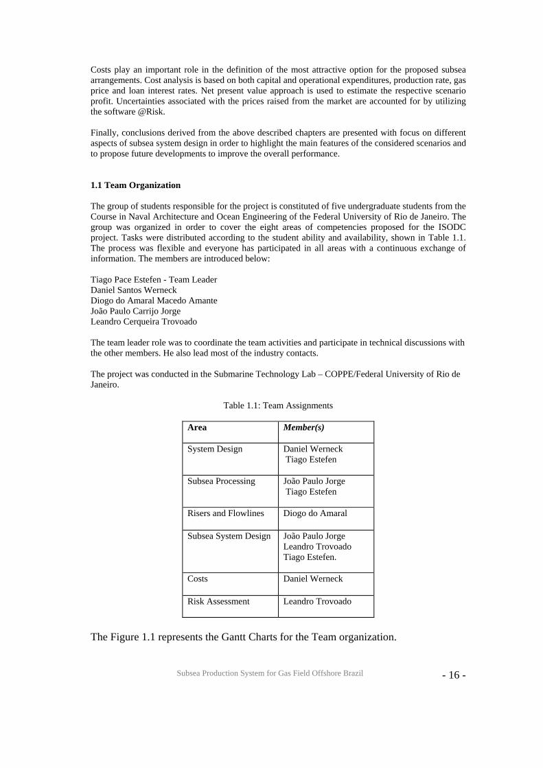
Table 1.1: Team Assignments
Area
Member(s)
System Design
Daniel Werneck Tiago Estefen
Subsea Processing
João Paulo Jorge Tiago Estefen
Risers and Flowlines
Diogo do Amaral
Subsea System Design João Paulo Jorge Leandro Trovoado Tiago Estefen.
Costs
Daniel Werneck
Risk Assessment
Leandro Trovoado
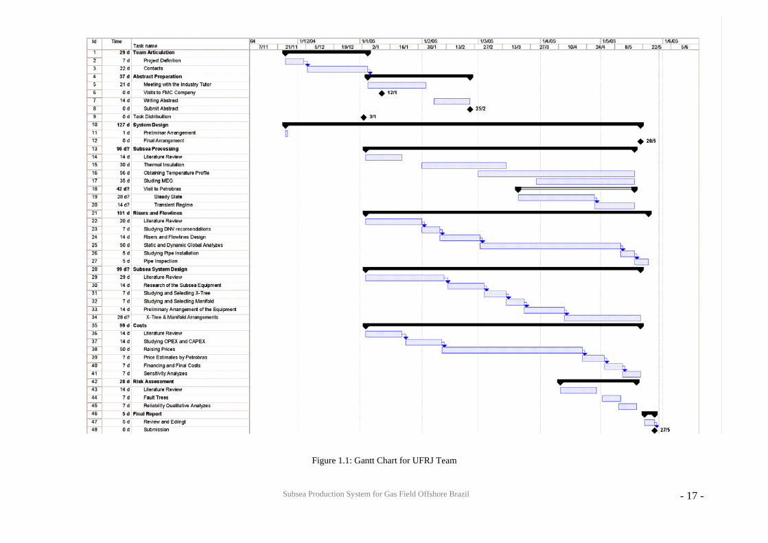
The Figure 1.1 represents the Gantt Charts for the Team organization.
Subsea Production System for Gas Field Offshore Brazil
- 17 -
Figure 1.1: Gantt Chart for UFRJ Team
Subsea Production System for Gas Field Offshore Brazil
- 18 -
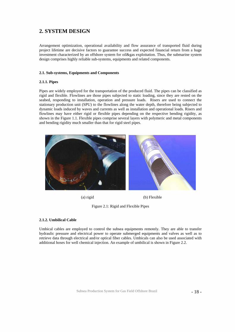
2. SYSTEM DESIGN Arrangement optimization, operational availability and flow assurance of transported fluid during project lifetime are decisive factors to guarantee success and expected financial return from a huge investment characterized by an offshore system for oil&gas exploitation. Thus, the submarine system design comprises highly reliable sub-systems, equipments and related components. 2.1. Sub-systems, Equipments and Components 2.1.1. Pipes Pipes are widely employed for the transportation of the produced fluid. The pipes can be classified as rigid and flexible. Flowlines are those pipes subjected to static loading, since they are rested on the seabed, responding to installation, operation and pressure loads. Risers are used to connect the stationary production unit (SPU) to the flowlines along the water depth, therefore being subjected to dynamic loads induced by waves and currents as well as installation and operational loads. Risers and flowlines may have either rigid or flexible pipes depending on the respective bending rigidity, as shown in the Figure 1.1. Flexible pipes comprise several layers with polymeric and metal components and bending rigidity much smaller than that for rigid steel pipes.
(a) rigid (b) Flexible
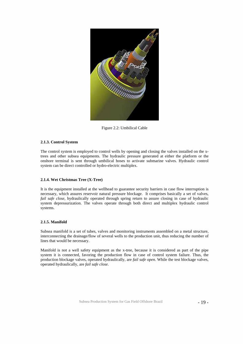
Figure 2.1: Rigid and Flexible Pipes 2.1.2. Umbilical Cable Umbical cables are employed to control the subsea equipments remotely. They are able to transfer hydraulic pressure and electrical power to operate submerged equipments and valves as well as to retrieve data through electrical and/or optical fiber cables. Umbicals can also be used associated with additional hoses for well chemical injection. An example of umbilical is shown in Figure 2.2.
Subsea Production System for Gas Field Offshore Brazil
- 19 -
Figure 2.2: Umbilical Cable 2.1.3. Control System The control system is employed to control wells by opening and closing the valves installed on the x-trees and other subsea equipments. The hydraulic pressure generated at either the platform or the onshore terminal is sent through umbilical hoses to activate submarine valves. Hydraulic control system can be direct controlled or hydro-electric multiplex. 2.1.4. Wet Christmas Tree (X-Tree) It is the equipment installed at the wellhead to guarantee security barriers in case flow interruption is necessary, which assures reservoir natural pressure blockage. It comprises basically a set of valves, fail safe close, hydraulically operated through spring return to assure closing in case of hydraulic system depressurization. The valves operate through both direct and multiplex hydraulic control systems. 2.1.5. Manifold Subsea manifold is a set of tubes, valves and monitoring instruments assembled on a metal structure, interconnecting the drainage/flow of several wells to the production unit, thus reducing the number of lines that would be necessary. Manifold is not a well safety equipment as the x-tree, because it is considered as part of the pipe system it is connected, favoring the production flow in case of control system failure. Thus, the production blockage valves, operated hydraulically, are fail safe open. While the test blockage valves, operated hydraulically, are fail safe close.
Subsea Production System for Gas Field Offshore Brazil
- 20 -
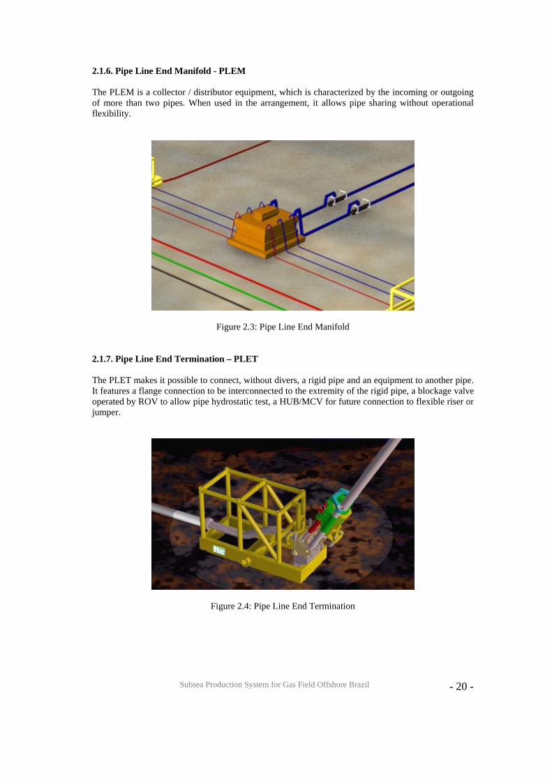
2.1.6. Pipe Line End Manifold - PLEM The PLEM is a collector / distributor equipment, which is characterized by the incoming or outgoing of more than two pipes. When used in the arrangement, it allows pipe sharing without operational flexibility.
Figure 2.3: Pipe Line End Manifold 2.1.7. Pipe Line End Termination – PLET The PLET makes it possible to connect, without divers, a rigid pipe and an equipment to another pipe. It features a flange connection to be interconnected to the extremity of the rigid pipe, a blockage valve operated by ROV to allow pipe hydrostatic test, a HUB/MCV for future connection to flexible riser or jumper.
Figure 2.4: Pipe Line End Termination
Subsea Production System for Gas Field Offshore Brazil
- 21 -
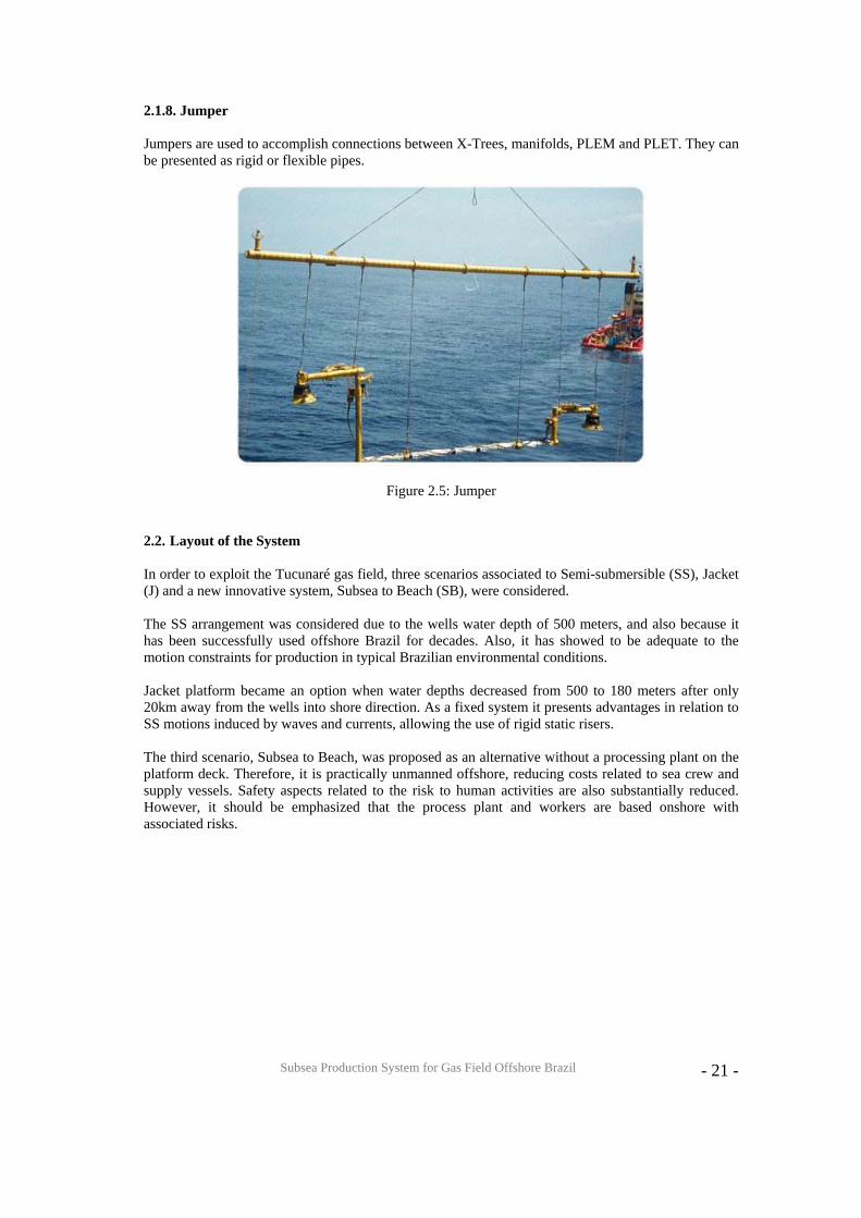
2.1.8. Jumper Jumpers are used to accomplish connections between X-Trees, manifolds, PLEM and PLET. They can be presented as rigid or flexible pipes.
Figure 2.5: Jumper 2.2. Layout of the System In order to exploit the Tucunaré gas field, three scenarios associated to Semi-submersible (SS), Jacket (J) and a new innovative system, Subsea to Beach (SB), were considered. The SS arrangement was considered due to the wells water depth of 500 meters, and also because it has been successfully used offshore Brazil for decades. Also, it has showed to be adequate to the motion constraints for production in typical Brazilian environmental conditions. Jacket platform became an option when water depths decreased from 500 to 180 meters after only 20km away from the wells into shore direction. As a fixed system it presents advantages in relation to SS motions induced by waves and currents, allowing the use of rigid static risers. The third scenario, Subsea to Beach, was proposed as an alternative without a processing plant on the platform deck. Therefore, it is practically unmanned offshore, reducing costs related to sea crew and supply vessels. Safety aspects related to the risk to human activities are also substantially reduced. However, it should be emphasized that the process plant and workers are based onshore with associated risks.
Subsea Production System for Gas Field Offshore Brazil
- 22 -
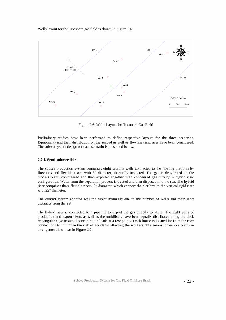
Wells layout for the Tucunaré gas field is shown in Figure 2.6
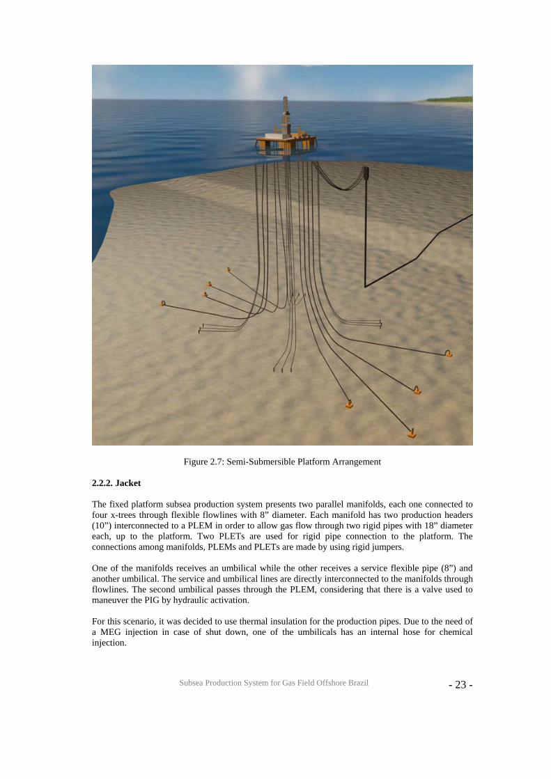
Figure 2.6: Wells Layout for Tucunaré Gas Field Preliminary studies have been performed to define respective layouts for the three scenarios. Equipments and their distribution on the seabed as well as flowlines and riser have been considered. The subsea system design for each scenario is presented below. 2.2.1. Semi-submersible The subsea production system comprises eight satellite wells connected to the floating platform by flowlines and flexible risers with 8” diameter, thermally insulated. The gas is dehydrated on the process plant, compressed and then exported together with condensed gas through a hybrid riser configuration. Water from the separation process is treated and then disposed into the sea. The hybrid riser comprises three flexible risers, 8” diameter, which connect the platform to the vertical rigid riser with 22” diameter. The control system adopted was the direct hydraulic due to the number of wells and their short distances from the SS. The hybrid riser is connected to a pipeline to export the gas directly to shore. The eight pairs of production and export risers as well as the umbilicals have been equally distributed along the deck rectangular edge to avoid concentration loads at a few points. Deck house is located far from the riser connections to minimize the risk of accidents affecting the workers. The semi-submersible platform arrangement is shown in Figure 2.7.
0 500 1000
500 m
505 m
495 m
SCALE (Meter)
W-1
W-7
W-6
W-5
W-4
W-3
W-2
W-8
SHORE DIRECTION
Subsea Production System for Gas Field Offshore Brazil
- 23 -
Figure 2.7: Semi-Submersible Platform Arrangement 2.2.2. Jacket The fixed platform subsea production system presents two parallel manifolds, each one connected to four x-trees through flexible flowlines with 8” diameter. Each manifold has two production headers (10”) interconnected to a PLEM in order to allow gas flow through two rigid pipes with 18” diameter each, up to the platform. Two PLETs are used for rigid pipe connection to the platform. The connections among manifolds, PLEMs and PLETs are made by using rigid jumpers. One of the manifolds receives an umbilical while the other receives a service flexible pipe (8”) and another umbilical. The service and umbilical lines are directly interconnected to the manifolds through flowlines. The second umbilical passes through the PLEM, considering that there is a valve used to maneuver the PIG by hydraulic activation. For this scenario, it was decided to use thermal insulation for the production pipes. Due to the need of a MEG injection in case of shut down, one of the umbilicals has an internal hose for chemical injection.
Subsea Production System for Gas Field Offshore Brazil
- 24 -
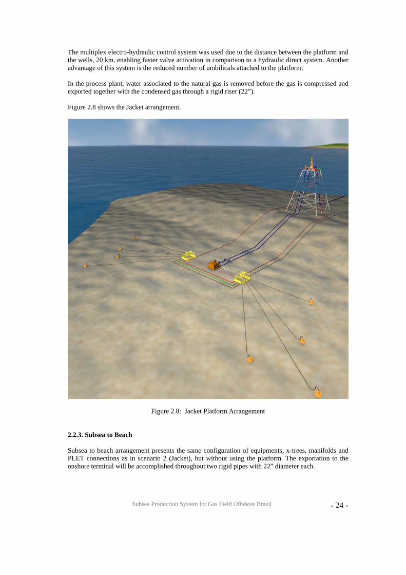
The multiplex electro-hydraulic control system was used due to the distance between the platform and the wells, 20 km, enabling faster valve activation in comparison to a hydraulic direct system. Another advantage of this system is the reduced number of umbilicals attached to the platform. In the process plant, water associated to the natural gas is removed before the gas is compressed and exported together with the condensed gas through a rigid riser (22”). Figure 2.8 shows the Jacket arrangement.
Figure 2.8: Jacket Platform Arrangement 2.2.3. Subsea to Beach Subsea to beach arrangement presents the same configuration of equipments, x-trees, manifolds and PLET connections as in scenario 2 (Jacket), but without using the platform. The exportation to the onshore terminal will be accomplished throughout two rigid pipes with 22” diameter each.
Subsea Production System for Gas Field Offshore Brazil
- 25 -
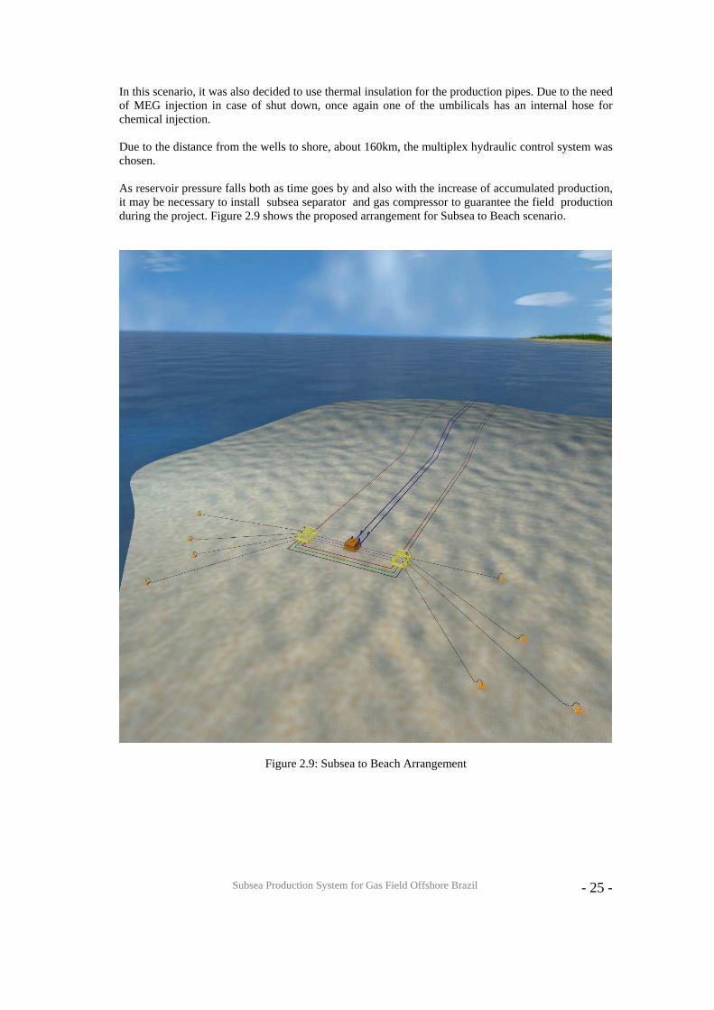
In this scenario, it was also decided to use thermal insulation for the production pipes. Due to the need of MEG injection in case of shut down, once again one of the umbilicals has an internal hose for chemical injection. Due to the distance from the wells to shore, about 160km, the multiplex hydraulic control system was chosen. As reservoir pressure falls both as time goes by and also with the increase of accumulated production, it may be necessary to install subsea separator and gas compressor to guarantee the field production during the project. Figure 2.9 shows the proposed arrangement for Subsea to Beach scenario.
Figure 2.9: Subsea to Beach Arrangement

Subsea Production System for Gas Field Offshore Brazil
- 26 -
3. SUBSEA PROCESSING This chapter describes the technical challenges and solutions of flow assurance for gas production in accordance to the environmental conditions of the analyzed field. The biggest problem when studying a gas field is to avoid the formation of hydrates. Two solutions were analyzed, thermal insulation and continuous injection of Mono Ethylene Glycol (MEG). In order to obtain thermal insulation that complies with project specifications, temperature profiles in steady-state production conditions for the three different scenarios will be initially calculated based on a theoretical approach. The pressure profile, in steady-state, will be determined using the computer program PIPESIM. The analyses of the transient regime will be carried out using the computer program OLGA. Shut down production and line depressurization will be simulated. After that, the continuous injection of thermodynamic inhibitor, MEG, and its volume needed to avoid the hydrate formation will be analyzed. 3.1. Hydrates Hydrates are ice-like solid crystalline normally formed at high pressure and low temperatures in the presence of water. They are the result of the combination of natural gas light component molecules with water molecules. These gather around the gas molecules, forming a sort of cavity that capsules the gas. Figure 3.1 illustrates a hydrate removed from a pipe.
Figure 3.1: Hydrate Plug Removed from a Gas Pipeline. Once defined gas composition, flow assurance study is summarized in three fundamental analyses: thermodynamic, fluid dynamic and heat transfer. The thermodynamic analysis defines state properties such as specific heat for constant pressure and constant volume (Cp and Cv) and specific mass (ρ). These will be used to determine pressure and temperature profile along the line. Therefore, with temperature and pressure data along the line, it is possible to determine hydrate formation points. In case there is hydrate formation, prevention and dissociation methods should be proposed. The most adopted methods to avoid hydrate formation are:
Subsea Production System for Gas Field Offshore Brazil
- 27 -
• Water removal; • Line heating; • Line depressurization; • Line thermal insulation; • Use of thermodynamic inhibitors.
3.2. Types of Thermal Insulation Pipeline thermal insulation is one of the means currently adopted to keep production free of hydrate formation and assure production flow. The definition of the thermal insulation is extremely peculiar to the particular submarine system in analysis (distances to be covered, well outflow, pressure and temperature data). Currently, several thermal insulation systems are known that vary according to the material used for assembly and insulation. Among them, the following can be highlighted:
i. Fully external insulation – insulation is placed directly on insulated surface and solid, synthetic and synthetic-composed materials are used. It is particularly appropriate for equipment with a more complex geometry.
ii. Multi-layer insulation – it is a kind of fully external insulation, generally composed by a solid layer and a foam layer, where each layer performs a specific function. The advantage of the multi-layer system is that the thickness and density of each layer can be customized to both project’s thermal and structural requirements. iii. Module insulation – it consists of pre-manufactured insulation sections mounted on the structure to be insulated without being directly attached to it. Synthetic and synthetic-composed materials are generally used for it. One of the advantages of this type of insulation is that it can be removed during its useful life. However, it has the disadvantage of possible presence of clearances due to faulty fit between the attached parts, which causes heat transfer through convection in these clearances, thus decreasing the insulation capacity. iv. Pipe-in-Pipe – it involves two tubes concentrically positioned, where empty space between them is filled up with insulating material. The main advantage of this scheme is the capacity to deal with high insulating capacity materials that cannot be used if they were not protected with an external pipeline. The main disadvantage is in set-up and manufacture costs in comparison with single wall pipes.
3.2.1. Thermal Insulation Adopted The thermal insulation proposed, polypropylene foam, for rigid pipes consists in a multi-layer anti-rusty protection applied to pipe surface. The surface has to be previously cleaned and prepared according to pre-set standards. This system is appropriate to offshore installations, due to its good mechanic and thermal resistance features, and it is generally used for water depths up to 600 meters. After a previous visual inspection of pipes and of pre-heating/ jetting of pipe external surface, the system is applied as description below.
• Primer (1st layer) The function of primer is to form a barrier thin layer closely bonded to the metal surface and with excellent chemical resistance properties. Pipe surface fully coating with primer layer provides both high resistance to the cathodic unbounded and a perfect chemical adherence between subsequent layers, providing the pipe with high resistance to coating peeling. It is applied by electrostatic guns.
Subsea Production System for Gas Field Offshore Brazil
- 28 -
• Adhesive (2nd layer) The function of the adhesive in coating is to optimize adhesion between the subsequent layer of polypropylene foam and the primer layer, through the combination of reactive effects, providing a perfect chemical adherence. It is applied by lateral extrusion.
• Polypropylene Foam (3rd. Layer)
Polypropylene foam provides excellent thermal resistance properties. The thickness of this layer depends on project’s requirements (function of global heat transfer coefficient, U value). It is applied by lateral extrusion.
• Polypropylene Solid (4th. Layer)
Polypropylene solid is the outer layer of this system. It provides system with protection against ultra-violet rays. It is applied by lateral extrusion.
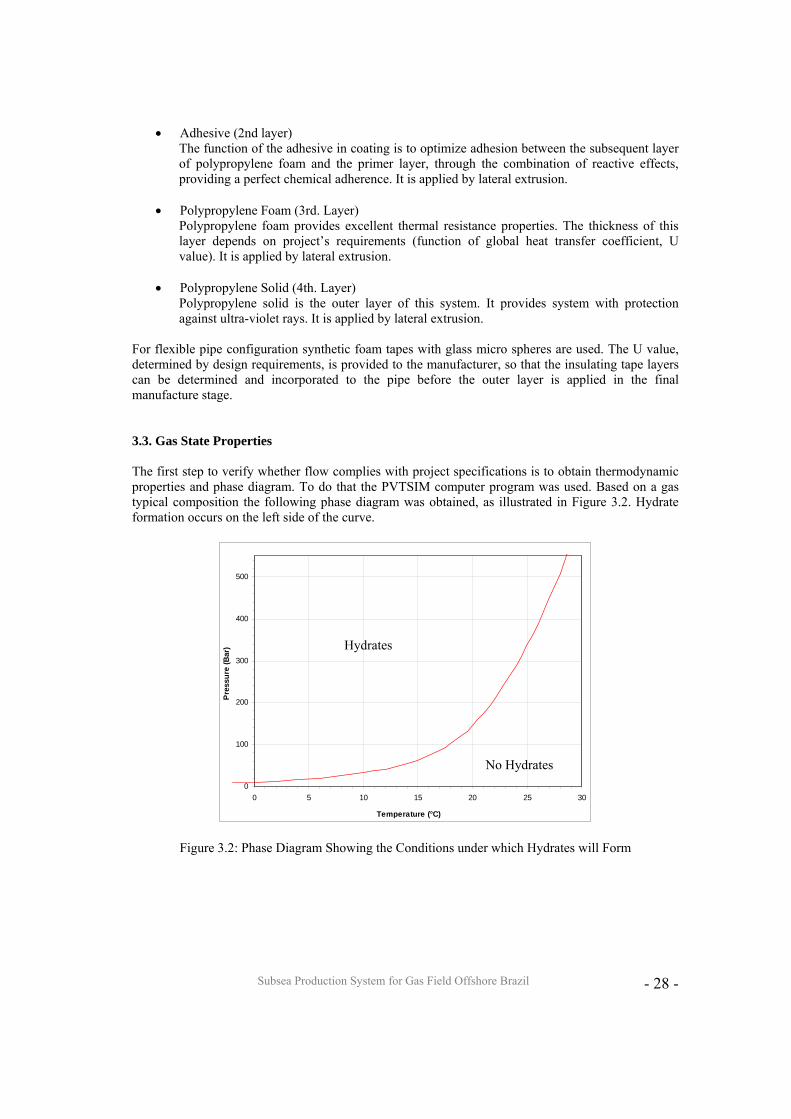
For flexible pipe configuration synthetic foam tapes with glass micro spheres are used. The U value, determined by design requirements, is provided to the manufacturer, so that the insulating tape layers can be determined and incorporated to the pipe before the outer layer is applied in the final manufacture stage. 3.3. Gas State Properties The first step to verify whether flow complies with project specifications is to obtain thermodynamic properties and phase diagram. To do that the PVTSIM computer program was used. Based on a gas typical composition the following phase diagram was obtained, as illustrated in Figure 3.2. Hydrate formation occurs on the left side of the curve.
Figure 3.2: Phase Diagram Showing the Conditions under which Hydrates will Form
0
100
200
300
400
500
0 5 10 15 20 25 30
Temperature (°C)
Pre
ssur
e (B
ar) Hydrates
No Hydrates
Subsea Production System for Gas Field Offshore Brazil
- 29 -
3.4. Temperature and Pressure Profile Determination 3.4.1. Temperature Profile Temperature profiles, in steady-state, were determined for the three scenarios. The theoretical analysis of the problem [1] considered some simplifying hypotheses.
• Flow steady-state and heat exchange (that is, no problem variable is dependent on time); • Unidimensional heat transfer (radial); • Mixture is idealized homogeneous, that is, monophase flow; • Only mixture temperature variation in the longitudinal direction is considered; • Physical properties for the mixture and the structure are independent on temperature and
pressure. Thus, the equation of heat in cylinder coordinates ( zr ,,θ ) for each pipe layer is given by:
01=⎟
⎠⎞
⎜⎝⎛
∂∂
∂∂
rTr
rr (3.1)
Heat transfer rate in radial direction (Fourier’s Law) is expressed by:
rTkAQ∂∂
−= (3.2)
where k is material thermal conductivity and A is the area normal to thermal flow. The analytical solution of the equation (3.1) allows the determination of temperature radial distribution T (r) on the pipe, in function of temperatures on inner and outer surface. It can also be proved that the heat transfer rate Q is constant, independent on r. The global heat transfer coefficient U of the composite structure is related to total thermal resistance. This can be defined as heat transfer rate per unit of inner surface area, iA , by temperature variation
between internal fluids (mixture, fT ) and external (sea water, wT ), as in the equation below.
)( wfi TTAQU−
= (3.3)
From the solution of equation (3.1), considering only heat flow per convection between the mixture and pipe inner wall and disregarding thermal resistance of contact and of the steel, the following expression for global heat transfer coefficient based on iA is written in the following equation.
⎟⎟⎠
⎞⎜⎜⎝
⎛
++++⎟
⎟⎠
⎞⎜⎜⎝
⎛
+++⎟⎟
⎠
⎞⎜⎜⎝
⎛++
=
foamsteel
solid
solid
i
foami
foam
foam
i
i
steel
steel
i
i ttRt
kR
tRt
kR
Rt
kR
h
U
1
1ln1ln1ln11
(3.4)
where
=ih convection heat transfer coefficient between mixture and pipe inner wall;
Subsea Production System for Gas Field Offshore Brazil
- 30 -
=steelk steel thermal conductivity (inner layer)
=foamk PP foam thermal conductivity (intermediary layer)
=solidk PP solid thermal conductivity (outer layer);
=iR inner radius;
=steelt steel thickness;
=foamt PP foam thickness;
=solidt PP solid thickness; The equation of mixture energy transportation, idealized as a homogeneous mixture, with one-dimensional flow in steady-state, can be written as:
))(2( wfif
pff TTRUds
dTcm −−= π& (3.5)
where
fm& = mass flow rate of the mixture;
pfc = specific heat of the mixture;
fT = mixture temperature in a determined position along the pipeline;
wT = sea water temperature in a determined position along the pipeline;
U = global heat transfer coefficient. For the problem being studied, was chosen 0=s at well head. The equation (3.5) is an first order ordinary differential equation with constant coefficients that has a simple analytical solution, which can be obtained from initial condition fT = 0T in 0=s . The
solution is as follow:
( ) pff cmRUs
mm eTTTTπ2
0
−
−+= (3.6)
With a desired exit temperature endT at Ls = the value of U can be estimate by rearranging algebraically the solution (3.6).
LRcm
TTTTU
i
pff
m
m
π2ln
0
⋅⎟⎟⎠
⎞⎜⎜⎝
⎛−−
−= (3.7)
U values and temperature profiles for the three scenarios will be calculated. To obtain U and temperature profile, the program MATLAB 6.5, whose calculations are presented in the Appendix A.
Subsea Production System for Gas Field Offshore Brazil
- 31 -
3.4.2. Pressure Profile
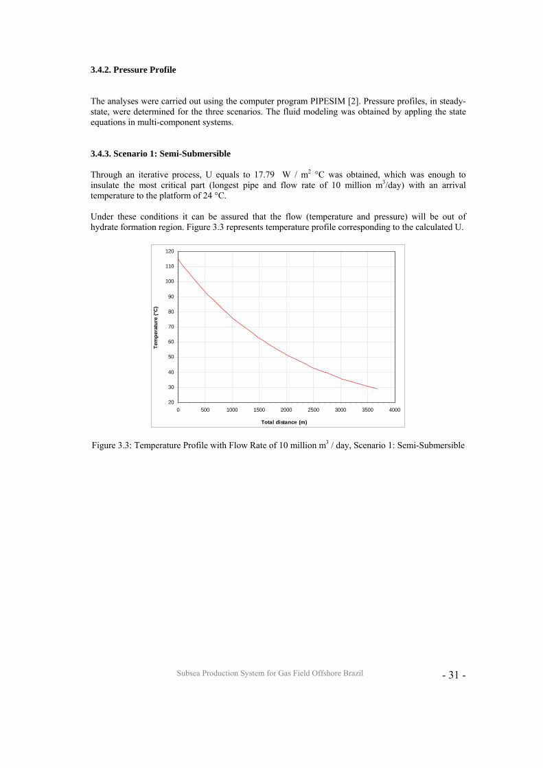
The analyses were carried out using the computer program PIPESIM [2]. Pressure profiles, in steady-state, were determined for the three scenarios. The fluid modeling was obtained by appling the state equations in multi-component systems. 3.4.3. Scenario 1: Semi-Submersible Through an iterative process, U equals to 17.79 W / m2 °C was obtained, which was enough to insulate the most critical part (longest pipe and flow rate of 10 million m3/day) with an arrival temperature to the platform of 24 °C. Under these conditions it can be assured that the flow (temperature and pressure) will be out of hydrate formation region. Figure 3.3 represents temperature profile corresponding to the calculated U.
20
30
40
50
60
70
80
90
100
110
120
0 500 1000 1500 2000 2500 3000 3500 4000
Total distance (m)
Tem
pera
ture
(°C)
Figure 3.3: Temperature Profile with Flow Rate of 10 million m3 / day, Scenario 1: Semi-Submersible
Subsea Production System for Gas Field Offshore Brazil
- 32 -
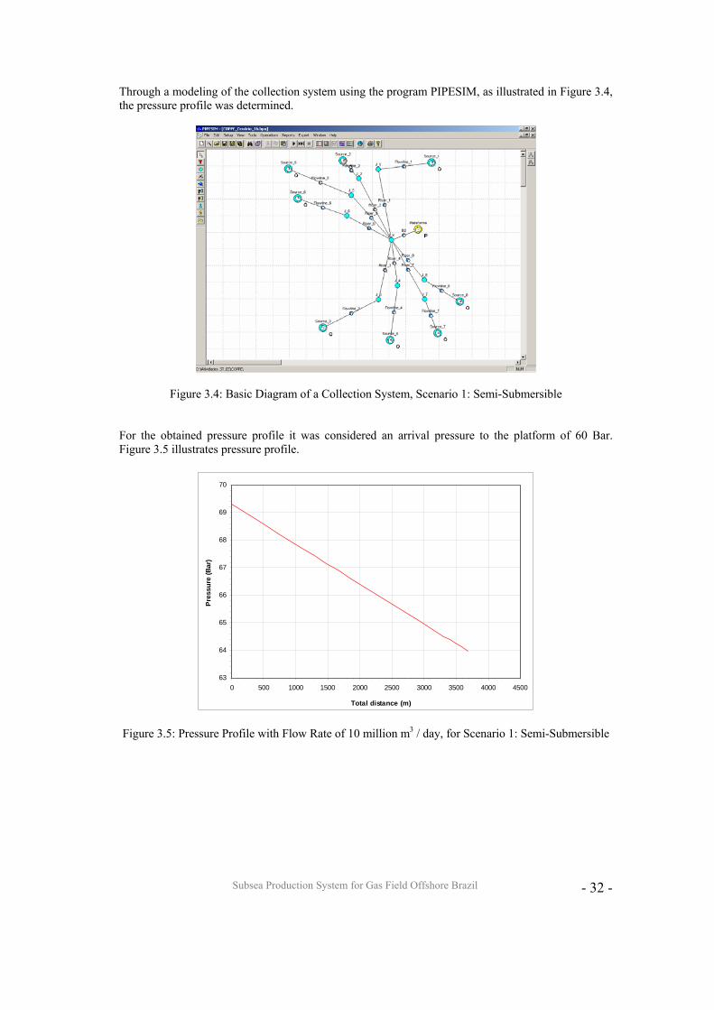
Through a modeling of the collection system using the program PIPESIM, as illustrated in Figure 3.4, the pressure profile was determined.
Figure 3.4: Basic Diagram of a Collection System, Scenario 1: Semi-Submersible For the obtained pressure profile it was considered an arrival pressure to the platform of 60 Bar. Figure 3.5 illustrates pressure profile.
63
64
65
66
67
68
69
70
0 500 1000 1500 2000 2500 3000 3500 4000 4500
Total distance (m)
Pres
sure
(Bar
)
Figure 3.5: Pressure Profile with Flow Rate of 10 million m3 / day, for Scenario 1: Semi-Submersible
Subsea Production System for Gas Field Offshore Brazil
- 33 -
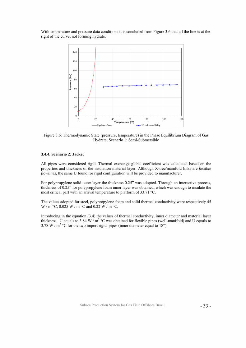
With temperature and pressure data conditions it is concluded from Figure 3.6 that all the line is at the right of the curve, not forming hydrate.
0
20
40
60
80
100
120
140
0 20 40 60 80 100 120Temperature (°C)
Pres
sure
(Bar
)
Hydrate Curve 10 million m3/day
Figure 3.6: Thermodynamic State (pressure, temperature) in the Phase Equilibrium Diagram of Gas Hydrate, Scenario 1: Semi-Submersible
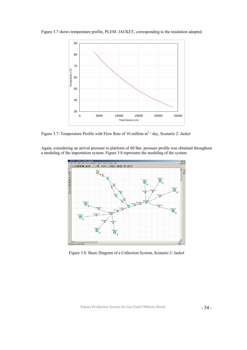
3.4.4. Scenario 2: Jacket All pipes were considered rigid. Thermal exchange global coefficient was calculated based on the properties and thickness of the insulation material layer. Although X-tree/manifold links are flexible flowlines, the same U found for rigid configuration will be provided to manufacturer. For polypropylene solid outer layer the thickness 0.25” was adopted. Through an interactive process, thickness of 0.25” for polypropylene foam inner layer was obtained, which was enough to insulate the most critical part with an arrival temperature to platform of 33.71 °C. The values adopted for steel, polypropylene foam and solid thermal conductivity were respectively 45 W / m °C, 0.025 W / m °C and 0.22 W / m °C. Introducing in the equation (3.4) the values of thermal conductivity, inner diameter and material layer thickness, U equals to 3.84 W / m2 °C was obtained for flexible pipes (well-manifold) and U equals to 3.78 W / m2 °C for the two import rigid pipes (inner diameter equal to 18”).
Subsea Production System for Gas Field Offshore Brazil
- 34 -
Figure 3.7 shows temperature profile, PLEM- JACKET, corresponding to the insulation adopted.
30
40
50
60
70
80
90
0 5000 10000 15000 20000 25000Total Distance (m)
Tem
pera
ture
(°C
)
Figure 3.7: Temperature Profile with Flow Rate of 10 million m3 / day, Scenario 2: Jacket
Again, considering an arrival pressure to platform of 60 Bar, pressure profile was obtained throughout a modeling of the importation system. Figure 3.8 represents the modeling of the system.
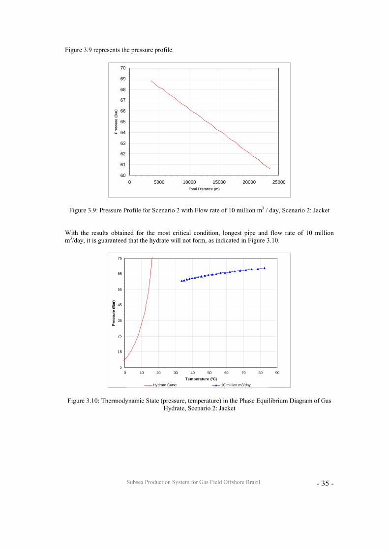
Figure 3.8: Basic Diagram of a Collection System, Scenario 2: Jacket
Subsea Production System for Gas Field Offshore Brazil
- 35 -
Figure 3.9 represents the pressure profile.
60
61
62
63
64
65
66
67
68
69
70
0 5000 10000 15000 20000 25000Total Distance (m)
Pre
ssur
e (B
ar)
Figure 3.9: Pressure Profile for Scenario 2 with Flow rate of 10 million m3 / day, Scenario 2: Jacket With the results obtained for the most critical condition, longest pipe and flow rate of 10 million m3/day, it is guaranteed that the hydrate will not form, as indicated in Figure 3.10.
5
15
25
35
45
55
65
75
0 10 20 30 40 50 60 70 80 90Temperature (°C)
Pre
ssur
e (B
ar)
Hydrate Curve 10 million m3/day Figure 3.10: Thermodynamic State (pressure, temperature) in the Phase Equilibrium Diagram of Gas
Hydrate, Scenario 2: Jacket
Subsea Production System for Gas Field Offshore Brazil
- 36 -
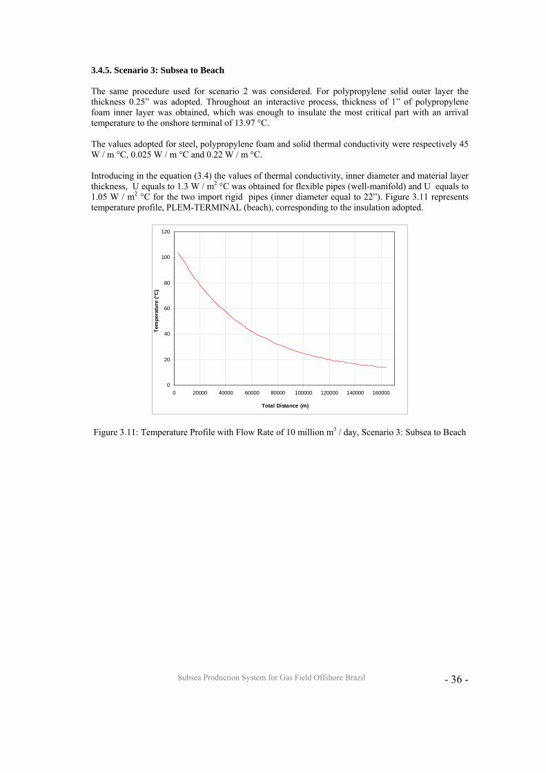
3.4.5. Scenario 3: Subsea to Beach The same procedure used for scenario 2 was considered. For polypropylene solid outer layer the thickness 0.25” was adopted. Throughout an interactive process, thickness of 1” of polypropylene foam inner layer was obtained, which was enough to insulate the most critical part with an arrival temperature to the onshore terminal of 13.97 °C. The values adopted for steel, polypropylene foam and solid thermal conductivity were respectively 45 W / m °C, 0.025 W / m °C and 0.22 W / m °C. Introducing in the equation (3.4) the values of thermal conductivity, inner diameter and material layer thickness, U equals to 1.3 W / m2 °C was obtained for flexible pipes (well-manifold) and U equals to 1.05 W / m2 °C for the two import rigid pipes (inner diameter equal to 22”). Figure 3.11 represents temperature profile, PLEM-TERMINAL (beach), corresponding to the insulation adopted.
0
20
40
60
80
100
120
0 20000 40000 60000 80000 100000 120000 140000 160000
Total Distance (m)
Tem
pera
ture
(°C)
Figure 3.11: Temperature Profile with Flow Rate of 10 million m3 / day, Scenario 3: Subsea to Beach
Subsea Production System for Gas Field Offshore Brazil
- 37 -
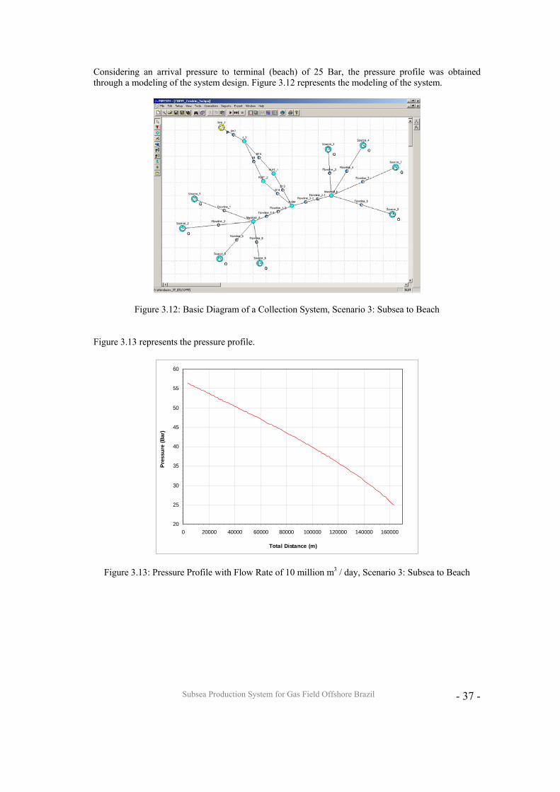
Considering an arrival pressure to terminal (beach) of 25 Bar, the pressure profile was obtained through a modeling of the system design. Figure 3.12 represents the modeling of the system.
Figure 3.12: Basic Diagram of a Collection System, Scenario 3: Subsea to Beach Figure 3.13 represents the pressure profile.
20
25
30
35
40
45
50
55
60
0 20000 40000 60000 80000 100000 120000 140000 160000
Total Distance (m)
Pre
ssur
e (B
ar)
Figure 3.13: Pressure Profile with Flow Rate of 10 million m3 / day, Scenario 3: Subsea to Beach
Subsea Production System for Gas Field Offshore Brazil
- 38 -
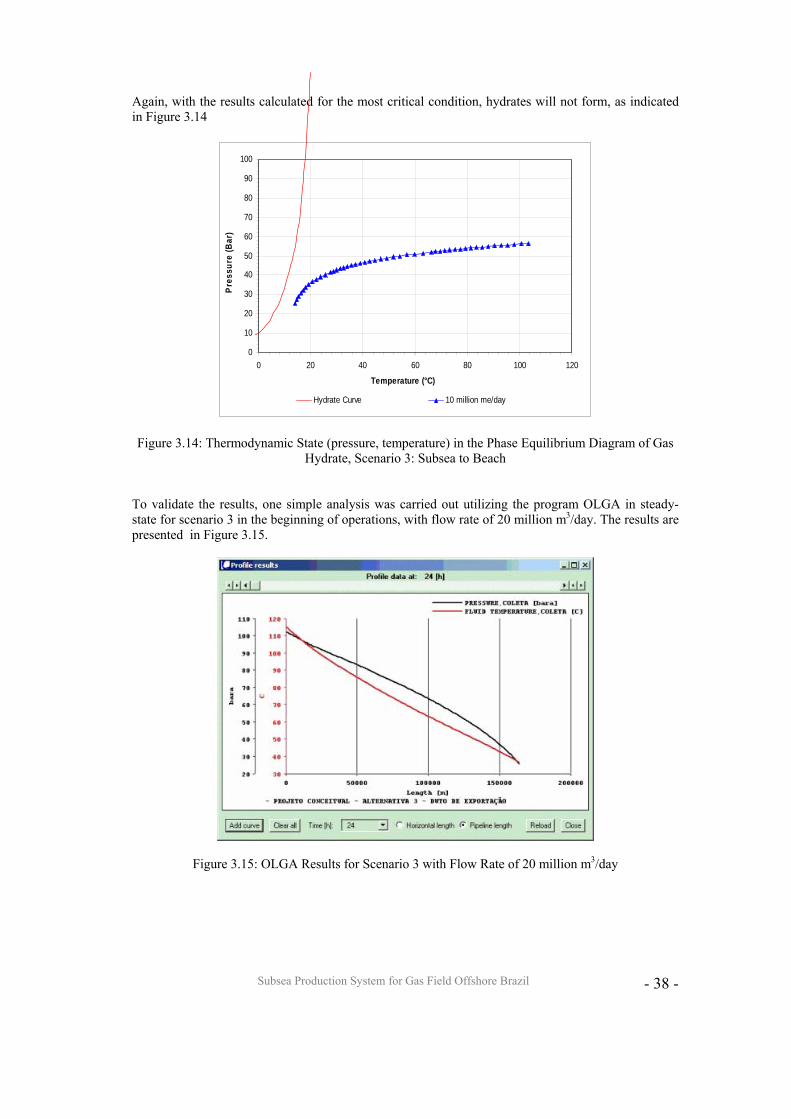
Again, with the results calculated for the most critical condition, hydrates will not form, as indicated in Figure 3.14
0
10
20
30
40
50
60
70
80
90
100
0 20 40 60 80 100 120
Temperature (°C)
Pres
sure
(Bar
)
Hydrate Curve 10 million me/day
Figure 3.14: Thermodynamic State (pressure, temperature) in the Phase Equilibrium Diagram of Gas Hydrate, Scenario 3: Subsea to Beach
To validate the results, one simple analysis was carried out utilizing the program OLGA in steady-state for scenario 3 in the beginning of operations, with flow rate of 20 million m3/day. The results are presented in Figure 3.15.
Figure 3.15: OLGA Results for Scenario 3 with Flow Rate of 20 million m3/day
Subsea Production System for Gas Field Offshore Brazil
- 39 -
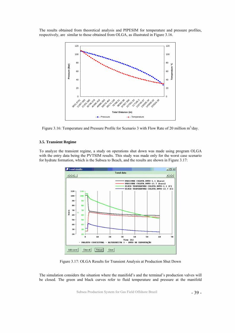
The results obtained from theoretical analysis and PIPESIM for temperature and pressure profiles, respectively, are similar to those obtained from OLGA, as illustrated in Figure 3.16.
0
20
40
60
80
100
120
3601
.6741
1160
7.093
2120
1.585
3079
6.078
4039
0.418
4998
5.093
5957
9.464
6917
4.139
7876
8.51
8836
2.88
9795
7.556
1075
51.93
1171
46.3
1267
40.97
1363
35.34
1459
30.02
1555
24.39
Total Distance (m)
Pres
sure
(Bar
)
0
20
40
60
80
100
120
Tem
pera
ture
°C
Pressure Temperature
Figure 3.16: Temperature and Pressure Profile for Scenario 3 with Flow Rate of 20 million m3/day.
3.5. Transient Regime To analyze the transient regime, a study on operations shut down was made using program OLGA with the entry data being the PVTSIM results. This study was made only for the worst case scenario for hydrate formation, which is the Subsea to Beach, and the results are shown in Figure 3.17:
Figure 3.17: OLGA Results for Transient Analysis at Production Shut Down The simulation considers the situation where the manifold’s and the terminal’s production valves will be closed. The green and black curves refer to fluid temperature and pressure at the manifold
Subsea Production System for Gas Field Offshore Brazil
- 40 -
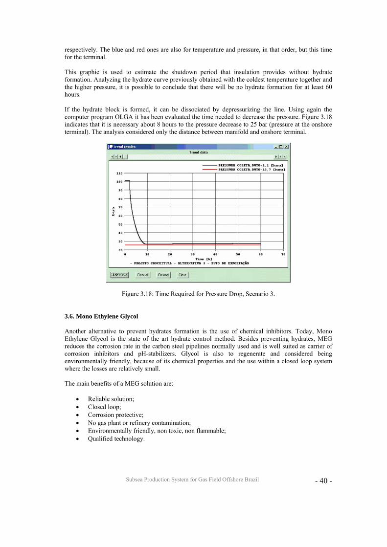
respectively. The blue and red ones are also for temperature and pressure, in that order, but this time for the terminal. This graphic is used to estimate the shutdown period that insulation provides without hydrate formation. Analyzing the hydrate curve previously obtained with the coldest temperature together and the higher pressure, it is possible to conclude that there will be no hydrate formation for at least 60 hours. If the hydrate block is formed, it can be dissociated by depressurizing the line. Using again the computer program OLGA it has been evaluated the time needed to decrease the pressure. Figure 3.18 indicates that it is necessary about 8 hours to the pressure decrease to 25 bar (pressure at the onshore terminal). The analysis considered only the distance between manifold and onshore terminal.
Figure 3.18: Time Required for Pressure Drop, Scenario 3. 3.6. Mono Ethylene Glycol Another alternative to prevent hydrates formation is the use of chemical inhibitors. Today, Mono Ethylene Glycol is the state of the art hydrate control method. Besides preventing hydrates, MEG reduces the corrosion rate in the carbon steel pipelines normally used and is well suited as carrier of corrosion inhibitors and pH-stabilizers. Glycol is also to regenerate and considered being environmentally friendly, because of its chemical properties and the use within a closed loop system where the losses are relatively small. The main benefits of a MEG solution are:
• Reliable solution; • Closed loop; • Corrosion protective; • No gas plant or refinery contamination; • Environmentally friendly, non toxic, non flammable; • Qualified technology.
Subsea Production System for Gas Field Offshore Brazil
- 41 -
In a closed loop system, Rich MEG arriving at the production unit must be regenerated to Lean MEG quality, 90-95 wt% MEG, before being re-injected at the subsea producers. There are two ways to do that:
I-Regeneration by evaporating water only. The MEG is returned to 90-95 wt% by boiling off the water at temperatures around 150°C. All salts and non-volatile chemicals remain in the MEG and are accumulated, if there is a continuous supply;
II-Full reclamation, which is an alternative if there is a “significant” formation water production. This is a low-pressure (100 to 150 mbar) that runs about 110°C. Both MEG and water are evaporated in a boiler and distilled to give 90-95 wt% Lean MEG and pure water. All salts and non-volatile components remain in the boiler and can be handle in different ways. Salts that precipitate in the boiler can be separated out, while small particles and soluble chemicals are more difficult to remove.
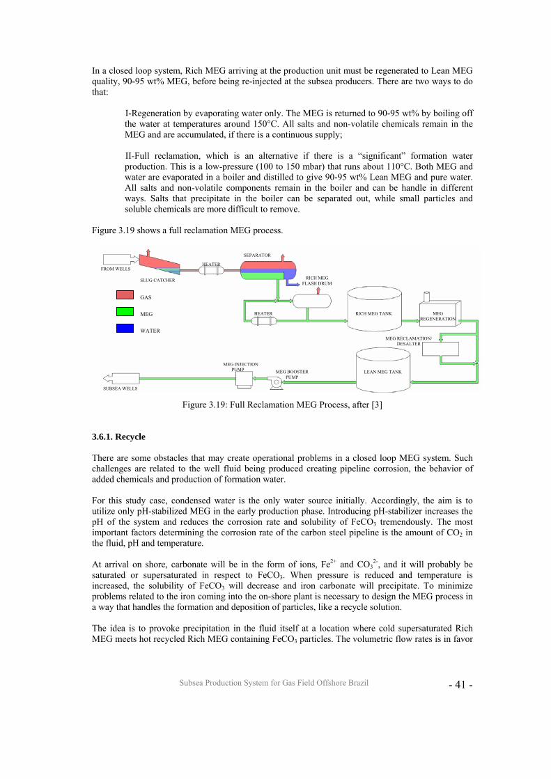
Figure 3.19 shows a full reclamation MEG process.
Figure 3.19: Full Reclamation MEG Process, after [3] 3.6.1. Recycle There are some obstacles that may create operational problems in a closed loop MEG system. Such challenges are related to the well fluid being produced creating pipeline corrosion, the behavior of added chemicals and production of formation water. For this study case, condensed water is the only water source initially. Accordingly, the aim is to utilize only pH-stabilized MEG in the early production phase. Introducing pH-stabilizer increases the pH of the system and reduces the corrosion rate and solubility of FeCO3 tremendously. The most important factors determining the corrosion rate of the carbon steel pipeline is the amount of CO2 in the fluid, pH and temperature. At arrival on shore, carbonate will be in the form of ions, Fe2+ and CO3
2-, and it will probably be saturated or supersaturated in respect to FeCO3. When pressure is reduced and temperature is increased, the solubility of FeCO3 will decrease and iron carbonate will precipitate. To minimize problems related to the iron coming into the on-shore plant is necessary to design the MEG process in a way that handles the formation and deposition of particles, like a recycle solution. The idea is to provoke precipitation in the fluid itself at a location where cold supersaturated Rich MEG meets hot recycled Rich MEG containing FeCO3 particles. The volumetric flow rates is in favor
FROM WELLS
SLUG CATCHER
SEPARATOR
HEATER
HEATER
RICH MEG TANK MEG REGENERATION
LEAN MEG TANK
MEG RECLAMATION/ DESALTER
SUBSEA WELLS
MEG INJECTION PUMP MEG BOOSTER
PUMP
RICH MEG
FLASH DRUM
GAS
MEG
WATER
Subsea Production System for Gas Field Offshore Brazil
- 42 -
of the recycle stream, and heating takes place in the recycle loop itself to avoid high temperature difference across the heater. To avoid accumulation of particle in the system, one or more solutions can be used. Some particle removal alternatives are mentioned below:
• Use of filters; • Settling by gravity using the long retention times in large glycol storage tanks; • Use of centrifugal forces.
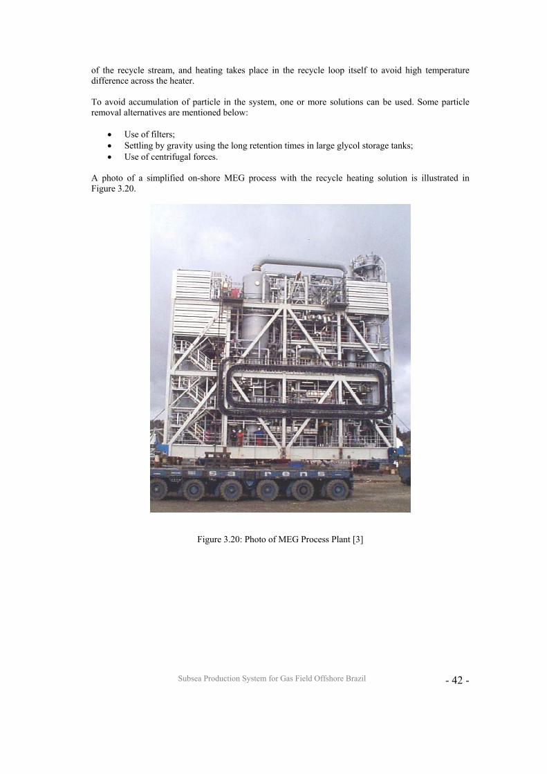
A photo of a simplified on-shore MEG process with the recycle heating solution is illustrated in Figure 3.20.
Figure 3.20: Photo of MEG Process Plant [3]
Subsea Production System for Gas Field Offshore Brazil
- 43 -
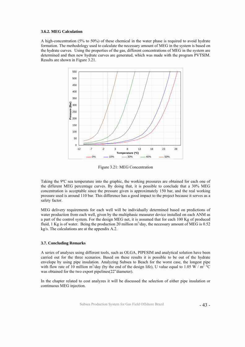
3.6.2. MEG Calculation A high-concentration (5% to 50%) of these chemical in the water phase is required to avoid hydrate formation. The methodology used to calculate the necessary amount of MEG in the system is based on the hydrate curves. Using the properties of the gas, different concentrations of MEG in the system are determined and then new hydrate curves are generated, which was made with the program PVTSIM. Results are shown in Figure 3.21.
0
50
100
150
200
250
300
350
400
450
500
550
-12 -7 -2 3 8 13 18 23 28Temperature (ºC)
Pres
sure
(Bar
)
0% 10% 30% 40% 50%
Figure 3.21: MEG Concentration Taking the 9ºC sea temperature into the graphic, the working pressures are obtained for each one of the different MEG percentage curves. By doing that, it is possible to conclude that a 30% MEG concentration is acceptable since the pressure given is approximately 150 bar, and the real working pressure used is around 110 bar. This difference has a good impact to the project because it serves as a safety factor. MEG delivery requirements for each well will be individually determined based on predictions of water production from each well, given by the multiphasic measurer device installed on each ANM as a part of the control system. For the design MEG net, it is assumed that for each 100 Kg of produced fluid, 1 Kg is of water. Being the production 20 million m3/day, the necessary amount of MEG is 0.52 kg/s. The calculations are at the appendix A.2. 3.7. Concluding Remarks A series of analyses using different tools, such as OLGA, PIPESIM and analytical solution have been carried out for the three scenarios. Based on these results it is possible to be out of the hydrate envelope by using pipe insulation. Analyzing Subsea to Beach for the worst case, the longest pipe with flow rate of 10 million m3/day (by the end of the design life), U value equal to 1.05 W / m2 °C was obtained for the two export pipelines(22”diameter). In the chapter related to cost analyzes it will be discussed the selection of either pipe insulation or continuous MEG injection.
Subsea Production System for Gas Field Offshore Brazil
- 44 -
4. FLOWLINES AND RISERS This chapter covers the design of flowlines and rigid risers for each of the scenarios. The diameters have been established considering flow and pressure values obtained from the reservoir data as previously discussed. The only scenario involving riser top movements is that associated with the semi-submersible platform, due to the action of waves and currents. Therefore, the riser response to these movements under extreme loading has been determined for this scenario. Pipes for both fixed platform and subsea to beach concepts are under static loading. Movements on the jacket main deck are neglected and subsea to beach has no riser. In this chapter was also accomplished a study for the pipe installation and description of the installation methods to be used. Pipelines need especial planning program for inspection and maintenance. In this context some equipments to detect geometric defects and corrosion as well as for hydrate removal are presented. 4.1. Design of Flowlines and Rigid Risers The design was accomplished using the ultimate limit state method, which is the main criterion related to rigid pipe local buckling (pipe wall bucking). DNV [5] recommendations were adopted for three different failures mode: local buckling due to bending moment, effective axial force and internal overpressure; local buckling due to longitudinal compressive strain and external overpressure; and propagation buckling. Limit states and design equations for this criterion were development based on experimental tests and structural reliability technique. The following nomenclature is used to define the criteria:
• Pc = collapse pressure • Pi = internal pressure • Pe = external pressure • Pp = plastic collapse pressure • Pel = elastic collapse pressure • t = nominal wall thickness of pipe • D = nominal outside diameter • E = Young`s modulus • ν = Poisson coefficient • σy = yield stress • f0 = ovality • ε = design compressive strain • εc = collapse compressive strain • γε = resistance factor, strain resistance • pld = local design pressure • Md = design bending moment • σu = tensile strength to be used in design • Sd = design effective axial force • ∆pd = design differential overpressure • Mp = plastic moment resistance • Sp = characteristic plastic axial force resistance • Pb(t) = burst pressure • αc = flow stress parameter
Subsea Production System for Gas Field Offshore Brazil
- 45 -
4.1.1. Local Buckling Due to Longitudinal Strain and External Overpressure Pipe members subjected to longitudinal compressive strain and external overpressure shall be designed to satisfy the following condition:
1
)(
8.0
≤
⋅
+⎟⎟⎟⎟
⎠
⎞
⎜⎜⎜⎜
⎝
⎛
mSC
C
e
C PP
γγγεε
ε
45≤tD and ei PP < (4.1)
In the analyzed scenarios, the effect of longitudinal deformation due to the bending can be neglected. Therefore, the equation is simplified as:
SCm
ce
PPγγ
≤ (4.2)
where: γm is the material resistance factor, γm = 1.15 γSC is the safety class resistance factor shown in the Table 4.1.
Table 4.1: Safety Class Resistance Factor, scγ
Safety Class Low Normal High γSC 1.046 1.138 1.308
High safety class has been assumed in the design. The external pressure is given by:
pe ρ.g.h.γP = (4.3) The pressure load effect factor, γp, is obtained from the Table 4.2 according to the limit state.
Table 4.2: Pressure Load Effect Factor
Limit States γP Serviceability (SLS) &
Ultimate (ULS) 1.05
Fatigue (FLS) 1.00
Accidental (ALS) 1.00
In this design γp = 1.00 was assumed. The characteristic collapse pressure (Pc) must be calculated by the following expression:
( ) ( )tDfPPPPPPP opelcpcelc =−− 22 (4.4)
where the elastic collapse pressure and plastic collapse pressure are given by:
Subsea Production System for Gas Field Offshore Brazil
- 46 -
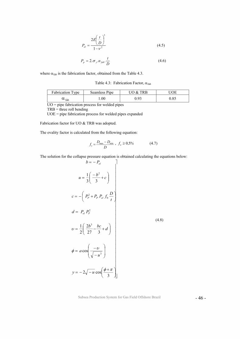
2
3
1
2
ν−
⎟⎠⎞
⎜⎝⎛
=DtE
Pel (4.5)
Dt..α.P fabyp σ2= (4.6)
where αfab is the fabrication factor, obtained from the Table 4.3.
Table 4.3: Fabrication Factor, αfab
Fabrication Type Seamless Pipe UO & TRB UOE
fabα 1.00 0.93 0.85 UO = pipe fabrication process for welded pipes TRB = three roll bending UOE = pipe fabrication process for welded pipes expanded Fabrication factor for UO & TRB was adopted. The ovality factor is calculated from the following equation:
DDDfo minmax −= , %,fo 50≥ (4.7)
The solution for the collapse pressure equation is obtained calculating the equations below:
⎥⎥⎥⎥⎥⎥⎥⎥⎥⎥⎥⎥⎥⎥⎥⎥⎥⎥⎥⎥⎥⎥⎥⎥⎥⎥⎥
⎦
⎤
⎟⎠⎞
⎜⎝⎛ +
−−=
⎟⎟
⎠
⎞
⎜⎜
⎝
⎛
−
−=
⎟⎟⎠
⎞⎜⎜⎝
⎛+−=
=
⎟⎠⎞
⎜⎝⎛ +−=
⎟⎟⎠
⎞⎜⎜⎝
⎛+
−=
−=
3cos2
cos
3272
21
331
3
3
2
02
2
πφ
υφ
υ
uy
ua
dbcb
PPd
tDfPPPc
cbu
Pb
Pel
elPP
el
(4.8)
Subsea Production System for Gas Field Offshore Brazil
- 47 -
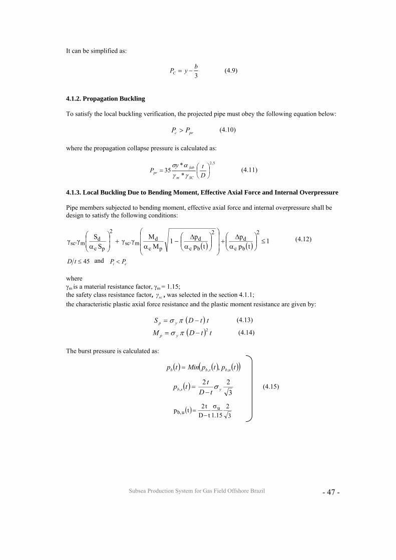
It can be simplified as:
3byPC −= (4.9)
4.1.2. Propagation Buckling To satisfy the local buckling verification, the projected pipe must obey the following equation below:
prc PP > (4.10) where the propagation collapse pressure is calculated as:
5,2
**
35 ⎟⎠⎞
⎜⎝⎛=Dty
PSCm
fabpr γγ
ασ (4.11)
4.1.3. Local Buckling Due to Bending Moment, Effective Axial Force and Internal Overpressure Pipe members subjected to bending moment, effective axial force and internal overpressure shall be design to satisfy the following conditions:
( ) ( ) 1tp
ptp
p1M
M.γγS
S.γγ2
bc
d2
bc
d
pc
dmsc
2
pc
dmsc ≤⎟⎟
⎠
⎞⎜⎜⎝
⎛α∆
+⎟⎟⎟
⎠
⎞
⎜⎜⎜
⎝
⎛
⎟⎟⎠
⎞⎜⎜⎝
⎛α∆
−α
+⎟⎟⎠
⎞⎜⎜⎝
⎛
α (4.12)
45≤tD and ei PP < where γm is a material resistance factor, γm = 1.15; the safety class resistance factor, scγ , was selected in the section 4.1.1; the characteristic plastic axial force resistance and the plastic moment resistance are given by:
( ) ttDS yp −= πσ (4.13)
( ) ttDM yp2−= πσ (4.14)
The burst pressure is calculated as:
( ) ( ) ( )( )tptpMintp ubsbb ,, ,=
( )3
22, ysb tD
ttp σ−
=
( )3
215.1tD
t2tp uu,b
σ−
=
(4.15)
Subsea Production System for Gas Field Offshore Brazil
- 48 -
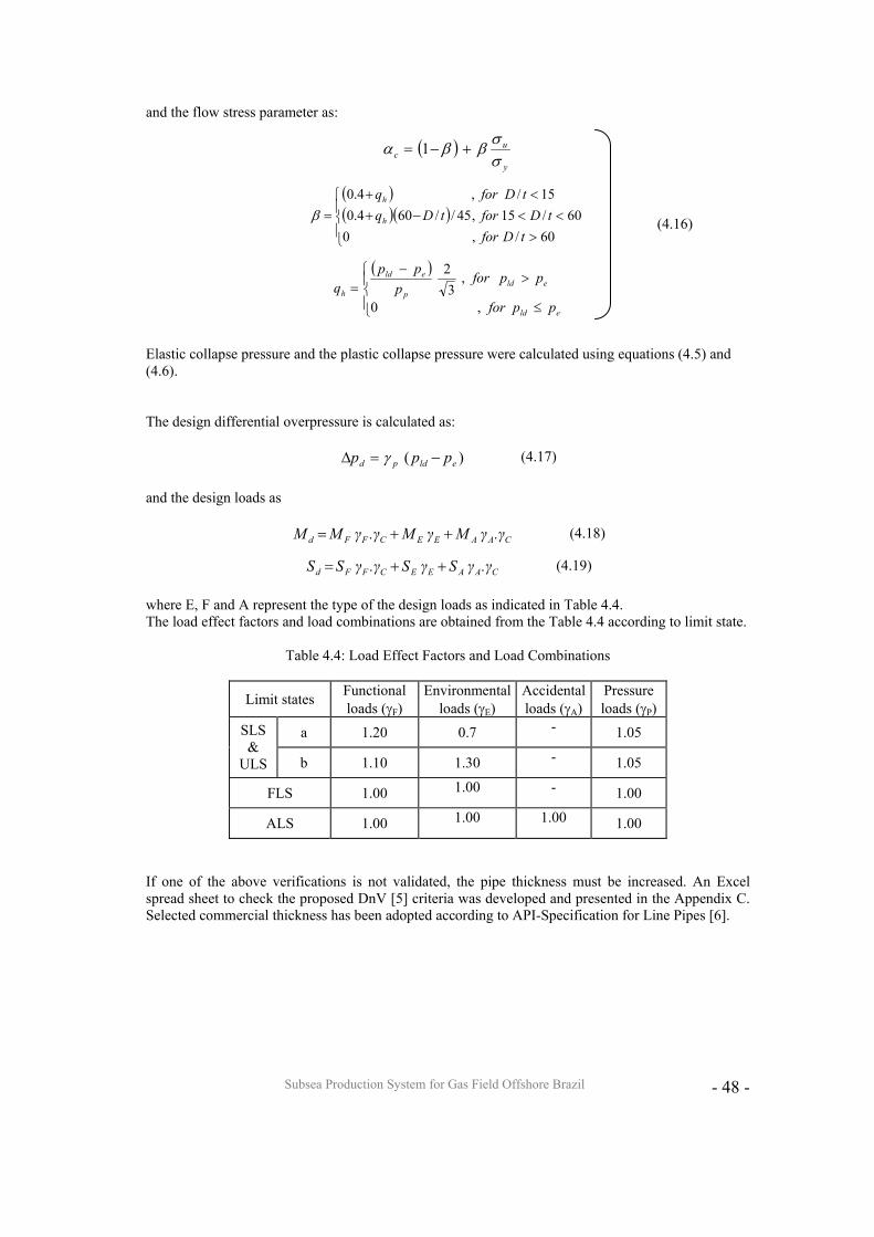
and the flow stress parameter as:
( )y
uc σ
σββα +−= 1
( )( )( )⎪⎩
⎪⎨
⎧
><<−+
<+=
60/,060/15,45//604.0
15/,4.0
tDfortDfortDq
tDforq
h
h
β
( )
⎪⎩
⎪⎨⎧
≤
>−
=
eld
eldp
eld
h
ppfor
ppforppp
q,0
,3
2
Elastic collapse pressure and the plastic collapse pressure were calculated using equations (4.5) and (4.6). The design differential overpressure is calculated as:
)( eldpd ppp −=∆ γ (4.17)
and the design loads as
CAAEECFFd .γγMγM.γγMM ++= (4.18)
CAAEECFFd .γγSγS.γγSS ++= (4.19)
where E, F and A represent the type of the design loads as indicated in Table 4.4. The load effect factors and load combinations are obtained from the Table 4.4 according to limit state.
Table 4.4: Load Effect Factors and Load Combinations
Limit states Functional loads (γF)
Environmental loads (γE)
Accidental loads (γA)
Pressure loads (γP)
a 1.20 0.7 - 1.05 SLS &
ULS b 1.10 1.30 - 1.05
FLS 1.00 1.00 - 1.00
ALS 1.00 1.00 1.00 1.00
If one of the above verifications is not validated, the pipe thickness must be increased. An Excel spread sheet to check the proposed DnV [5] criteria was developed and presented in the Appendix C. Selected commercial thickness has been adopted according to API-Specification for Line Pipes [6].
(4.16)
Subsea Production System for Gas Field Offshore Brazil
- 49 -
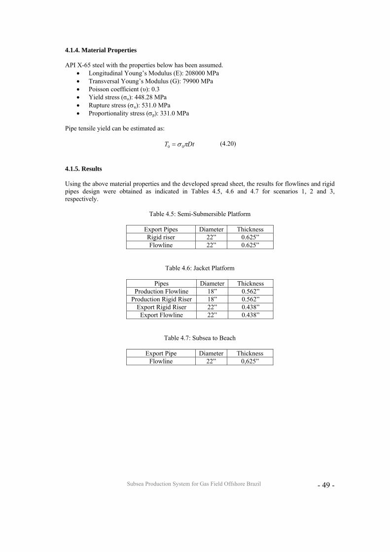
4.1.4. Material Properties API X-65 steel with the properties below has been assumed.
• Longitudinal Young’s Modulus (E): 208000 MPa • Transversal Young’s Modulus (G): 79900 MPa • Poisson coefficient (υ): 0.3 • Yield stress (σo): 448.28 MPa • Rupture stress (σu): 531.0 MPa • Proportionality stress (σp): 331.0 MPa
Pipe tensile yield can be estimated as:
DtT πσ 00 = (4.20) 4.1.5. Results Using the above material properties and the developed spread sheet, the results for flowlines and rigid pipes design were obtained as indicated in Tables 4.5, 4.6 and 4.7 for scenarios 1, 2 and 3, respectively.
Table 4.5: Semi-Submersible Platform
Export Pipes Diameter Thickness Rigid riser 22” 0.625” Flowline 22” 0.625”
Table 4.6: Jacket Platform
Pipes Diameter Thickness Production Flowline 18” 0.562”
Production Rigid Riser 18” 0.562” Export Rigid Riser 22” 0.438”
Export Flowline 22” 0.438”
Table 4.7: Subsea to Beach
Export Pipe Diameter Thickness Flowline 22” 0,625”
Subsea Production System for Gas Field Offshore Brazil
- 50 -
4.2 Riser Analyzes Considering Top Motions Analysis related to SS export and import (production) riser extreme loading conditions will be presented in the following sections. Extreme loadings from environmental conditions generate platform movements called offset. Static and dynamic global analyses for export and production risers were accomplished, taking into consideration wave and current extreme loadings with two return period combinations: centenary wave with decenary current and decenary wave with centenary current. The offset directions considered were near, far and transverse. ANFLEX computer program [7] developed jointly by COPPE and PETROBRAS was used for these analyses.
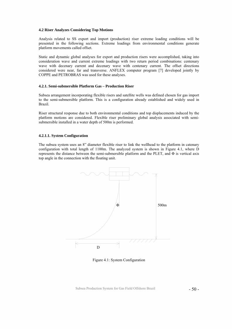
4.2.1. Semi-submersible Platform Gas – Production Riser Subsea arrangement incorporating flexible risers and satellite wells was defined chosen for gas import to the semi-submersible platform. This is a configuration already established and widely used in Brazil. Riser structural response due to both environmental conditions and top displacements induced by the platform motions are considered. Flexible riser preliminary global analysis associated with semi-submersible installed in a water depth of 500m is performed. 4.2.1.1. System Configuration The subsea system uses an 8” diameter flexible riser to link the wellhead to the platform in catenary configuration with total length of 1100m. The analyzed system is shown in Figure 4.1, where D represents the distance between the semi-submersible platform and the PLET, and Φ is vertical axis top angle in the connection with the floating unit.
Figure 4.1: System Configuration
500m
D
Φ
Subsea Production System for Gas Field Offshore Brazil
- 51 -
4.2.1.2. Relevant Parameters
Relevant parameters considered in the analysis are listed in Table 4.8. The adopted scenario was for 500m water depth. RAO´s and offsets used in the analysis are similar to those obtained from a similar platform to be installed in Campos Basin, offshore Brazil.
Table 4.8: Data for Static and Dynamic Analysis
Top angle 12º * Morrison coefficient 2.0 Drag coefficient 1.2 Riser total length (m) 1100
* Top angle value for the cases analyzed complies with technical specification [8].
4.2.1.3. Soil Data
Table 4.9 refers to soil data and presents the reaction coefficients used for superficial supporting condition, in compliance with Petrobras technical specifications [8].
Table 4.9: Soil Data
4.2.1.4. Structural Properties
Flexible riser and flex joint data are listed in Tables 4.10 and 4.11
Table 4.10: Flexible Pipe Data
Soil Modeling Horizontal
Axial friction coefficient 0.35
Lateral friction coefficient 0.5
Axial elastic deflection limit (m) 0.35
Lateral elastic deflection limit (m) 0.2597
Vertical spring stiffness (kN/m/m) 5.86
Length (m) 1100
Internal diameter (m) 0.2032
External diameter (m) 0.2896
Weigth in air (empty, kN/m) 1.031
Weigth in water (empty, kN/m) 0.3679
Axial stiffness (EA, kN) 625500
Bending stiffness (EI, kN.m2) 93.415
Subsea Production System for Gas Field Offshore Brazil
52
Table 4.11: Flexjoint Data
X stiffness (KN/m) 2.08x10⁸ Y stiffness (KN/m) 2.08x10⁸ Z stiffness (KN/m) 2.08x10⁸
RX stiffness (KN.m/deg) 4.5 RY stiffness (KN.m/deg) 4.5 RZ stiffness (KN.m/deg) 4.5
4.2.1.5. Environmental Data
Environmental data related to Campos Basin Intermediary Central (IC) region were used in compliance to technical specifications [9] for two extreme condition combinations corresponding to centenary wave with decenary current (CW/DC) and to decenary wave with centenary current (DW/CC). Both in collinear configuration. 4.2.1.6. Extreme Offset
Offset value used for global analysis takes the following errors into account:
• Platform positioning error, equal to 10 meters; • Submarine equipment positioning error (well, manifold) equal to 7.5 meters; • Static offset corresponding to 10% of the water depth.
4.2.1.7. Numerical Model
The numerical model adopted for analysis, as shown in Figure 4.2, has the following features:
• Top angle: 12 degrees • Number of segments: 3 • Flexible riser 1st segment length: 600m • Flexible riser 2nd segment length: 500m • Total length: 1100m • Boundary condition at platform interface: Flexjoint
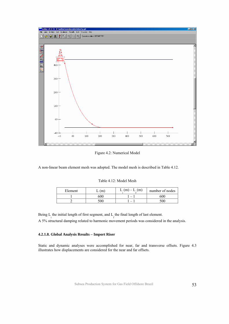
Subsea Production System for Gas Field Offshore Brazil
53
Figure 4.2: Numerical Model A non-linear beam element mesh was adopted. The model mesh is described in Table 4.12.
Table 4.12: Model Mesh
Element L (m) Li (m) – L
f (m) number of nodes
1 600 1 – 1 600 2 500 1 – 1 500
Being Li the initial length of first segment, and L
f the final length of last element.
A 5% structural damping related to harmonic movement periods was considered in the analysis.
4.2.1.8. Global Analysis Results – Import Riser
Static and dynamic analyses were accomplished for near, far and transverse offsets. Figure 4.3 illustrates how displacements are considered for the near and far offsets.
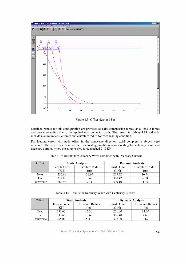
Subsea Production System for Gas Field Offshore Brazil
54
Figure 4.3: Offset Near and Far
Obtained results for this configuration are provided as axial compressive forces, axial tensile forces and curvature radius due to the applied environmental loads. The results in Tables 4.13 and 4.14 include maximum tensile forces and curvature radius for each loading condition.
For loading cases with static offset in the transverse direction, axial compressive forces were observed. The worst case was verified for loading condition corresponding to centenary wave and decenary current, where the compressive force reached 21.2 KN.
Table 4.13: Results for Centenary Wave combined with Decenary Current
Static Analysis Dynamic Analysis Offset Tensile Force
(KN) Curvature Radius
(m) Tensile Force
(KN) Curvature Radius
(m) Near 256.60 21.80 227.72 16.54 Far 332.00 9.49 380.42 6.58
Transverse 262.96 7.71 339.10 4.33
Table 4.14: Results for Decenary Wave with Centenary Current
Static Analysis Dynamic Analysis Offset
Tensile Force (KN)
Curvature Radius (m)
Tensile Force (KN)
Curvature Radius (m)
Near 256.60 17.30 221.00 14.20 Far 333.60 10.69 376.40 7.60
Transverse 265.00 5.43 328.30 3.69
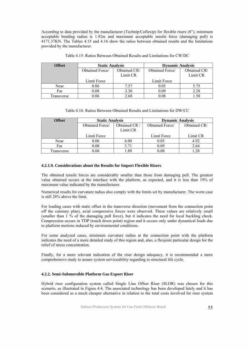
Subsea Production System for Gas Field Offshore Brazil
55
According to data provided by the manufacturer (Technip/Coflexip) for flexible risers (8”), minimum acceptable bending radius is 1.92m and maximum acceptable tensile force (damaging pull) is 4171.37KN. The Tables 4.15 and 4.16 show the ratios between obtained results and the limitations provided by the manufacturer.
Table 4.15: Ratios Between Obtained Results and Limitations for CW/DC
Static Analysis Dynamic Analysis Offset Obtained Force/
Limit Force
Obtained CR/ Limit CR
Obtained Force/
Limit Force
Obtained CR/ Limit CR
Near 0.06 7.57 0.05 5.75 Far 0.08 3.30 0.09 2.28
Transverse 0.06 2.68 0.08 1.50
Table 4.16: Ratios Between Obtained Results and Limitations for DW/CC
Static Analysis Dynamic Analysis Offset Obtained Force/
Limit Force
Obtained CR / Limit CR
Obtained Force/
Limit Force
Obtained CR/
Limit CR Near 0.06 6.00 0.05 4.92 Far 0.08 3.71 0.09 2.64
Transverse 0.06 1.89 0.08 1.28 4.2.1.9. Considerations about the Results for Import Flexible Risers The obtained tensile forces are considerably smaller than those from damaging pull. The greatest value obtained occurs at the interface with the platform, as expected, and it is less than 19% of maximum value indicated by the manufacturer.
Numerical results for curvature radius also comply with the limits set by manufacturer. The worst case is still 28% above the limit.
For loading cases with static offset in the transverse direction (movement from the connection point off the catenary plan), axial compressive forces were observed. These values are relatively small (smaller than 1 % of the damaging pull force), but it indicates the need for local buckling check. Compression occurs in TDP (touch down point) region and it occurs only under dynamical loads due to platform motions induced by environmental conditions.
For some analyzed cases, minimum curvature radius at the connection point with the platform indicates the need of a more detailed study of this region and, also, a flexjoint particular design for the relief of stress concentration.
Finally, for a more relevant indication of the riser design adequacy, it is recommended a more comprehensive study to assure system serviceability regarding to structural life cycle.
4.2.2. Semi-Submersible Platform Gas Export Riser Hybrid riser configuration system called Single Line Offset Riser (SLOR) was chosen for this scenario, as illustrated in Figure 4.4. The associated technology has been developed lately and it has been considered as a much cheaper alternative in relation to the total costs involved for riser system
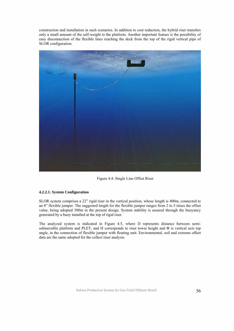
Subsea Production System for Gas Field Offshore Brazil
56
construction and installation in such scenarios. In addition to cost reduction, the hybrid riser transfers only a small amount of the self-weight to the platform. Another important feature is the possibility of easy disconnection of the flexible lines reaching the deck from the top of the rigid vertical pipe of SLOR configuration.
Figure 4.4: Single Line Offset Riser
4.2.2.1. System Configuration SLOR system comprises a 22” rigid riser in the vertical position, whose length is 400m, connected to an 8” flexible jumper. The suggested length for the flexible jumper ranges from 2 to 5 times the offset value, being adopted 300m in the present design. System stability is assured through the buoyancy generated by a buoy installed at the top of rigid riser. The analyzed system is indicated in Figure 4.5, where D represents distance between semi-submersible platform and PLET, and H corresponds to riser tower height and Φ is vertical axis top angle, in the connection of flexible jumper with floating unit. Environmental, soil and extreme offset data are the same adopted for the collect riser analysis.
Subsea Production System for Gas Field Offshore Brazil
57
Figure 4.5: System Configuration
4.2.2.2. Relevant Analysis Parameters
RAO´s and offsets were the same adopted for the collect riser analysis. Other relevant parameters are indicated in Table 4.17.
Table 4.17: Data for Static and Dynamic Analyzes
Top angle 12º * Morrison coefficient 2.0 Drag coefficient 1.2 Riser total length (m) 700
* Top angle value for the analyzed cases complies with Petrobras technical specifications [9]. 4.2.2.3. Structural Properties
Tables 4.18 to 4.21 list the main structural data associated with rigid pipe, flexible pipe, buoy and flexjoint, respectively.
Table 4.18: Rigid Pipe Data
Length (m) 400
Internal diameter (m) 0.52705
External diameter (m) 0.5588
Elastic modulus (E, kN/m2) 204000000
Hydrodynamic diameter (m) 0.5588
500 m
H
Φ
D
Subsea Production System for Gas Field Offshore Brazil
58
Table 4.19: Flexible Pipe Data
Table 4.20: Buoy Data
* The buoyance force was calculated as: Buoyance force (T) = 2 Psub (4.12) Psub
= Psteel
+ Pfluid– Psubvol (4.13)
where: Psub= submerse weight (obtained from ANFLEX program) Psteel= steel weight Pfluid
= internal fluid weight
Psubvol = submerse volume weight
Table 4.21: Flexjoint data
X stiffness (KN/m) 2.08.108 Y stiffness (KN/m) 2.08.108 Z stiffness (KN/m) 2.08.108 RX stiffness (KN.m/deg) 4.5 RY stiffness (KN.m/deg) 4.5 RZ stiffness (KN.m/deg) 4.5
4.2.2.4. Numerical Model
The numerical model adopted for analysis, as shown in Figure 4.6, has the following features:
• Top angle: 12º
Length (m) 300
Internal diameter (m) 0.2032
External diameter (m) 0.2896
Weight in air (empty, kN/m) 1.031
Weight in water (empty, kN/m) 0.3679
Axial stiffness (EA, kN) 625500
Bending stiffness (EI, kN.m2) 93.415
Buoyancy force (kN) * 3230 Weight (kN) 386
Area X (m2) 95.4
Area Y (m2) 95.4
Area Z (m2) 22.1
Morison inertia coefficient 2.0 Morison drag coefficient 1.88
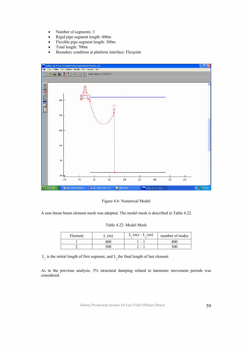
Subsea Production System for Gas Field Offshore Brazil
59
• Number of segments: 3 • Rigid pipe segment length: 400m • Flexible pipe segment length: 300m • Total length: 700m • Boundary condition at platform interface: Flexjoint
Figure 4.6: Numerical Model
A non-linear beam element mesh was adopted. The model mesh is described in Table 4.22.
Table 4.22: Model Mesh
Element L (m) L
i (m) – L
f (m) number of nodes
1 400 1 – 1 400 2 300 1 – 1 300
L
i is the initial length of first segment, and L
f the final length of last element.
As in the previous analysis, 5% structural damping related to harmonic movement periods was considered.
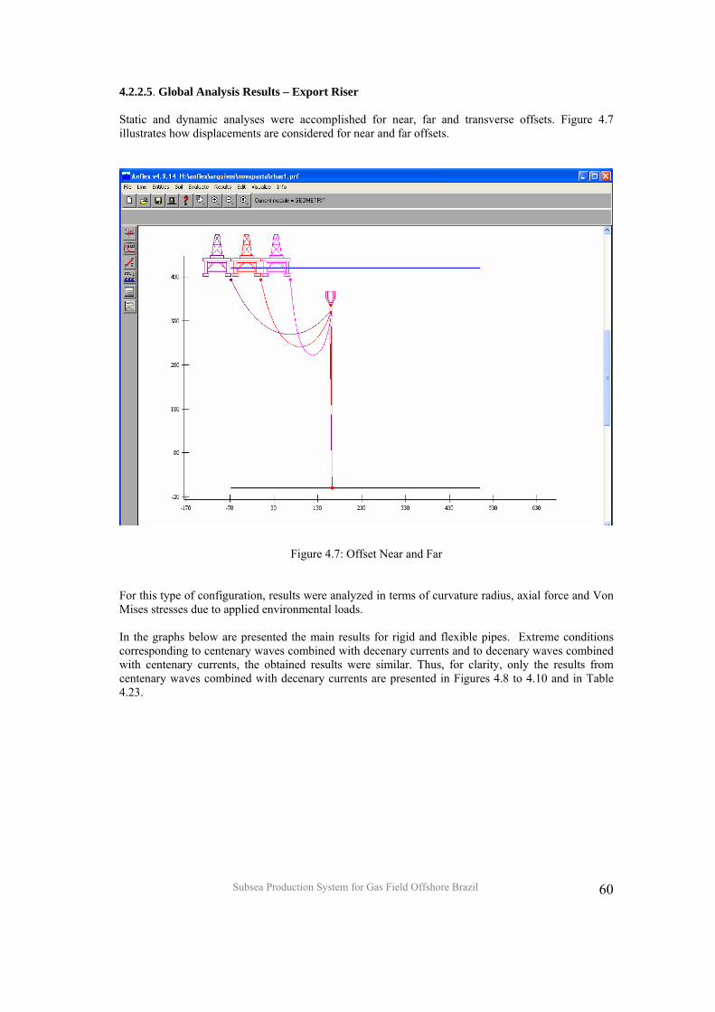
Subsea Production System for Gas Field Offshore Brazil
60
4.2.2.5. Global Analysis Results – Export Riser Static and dynamic analyses were accomplished for near, far and transverse offsets. Figure 4.7 illustrates how displacements are considered for near and far offsets.
Figure 4.7: Offset Near and Far For this type of configuration, results were analyzed in terms of curvature radius, axial force and Von Mises stresses due to applied environmental loads. In the graphs below are presented the main results for rigid and flexible pipes. Extreme conditions corresponding to centenary waves combined with decenary currents and to decenary waves combined with centenary currents, the obtained results were similar. Thus, for clarity, only the results from centenary waves combined with decenary currents are presented in Figures 4.8 to 4.10 and in Table 4.23.
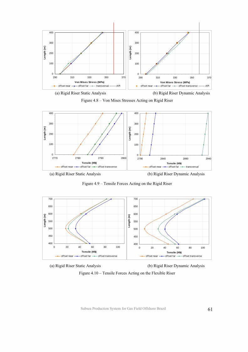
Subsea Production System for Gas Field Offshore Brazil
61
(a) Rigid Riser Static Analysis (b) Rigid Riser Dynamic Analysis
Figure 4.8 – Von Mises Stresses Acting on Rigid Riser
(a) Rigid Riser Static Analysis (b) Rigid Riser Dynamic Analysis
Figure 4.9 – Tensile Forces Acting on the Rigid Riser
(a) Rigid Riser Static Analysis (b) Rigid Riser Dynamic Analysis
Figure 4.10 – Tensile Forces Acting on the Flexible Riser
0
100
200
300
400
2770 2780 2790 2800
Tensile (KN)
Leng
th (m
)
offset near offset far offset transverse
0
100
200
300
400
2790 2840 2890 2940
Tensile (KN)
Leng
th (m
)
offset near offset far transversal
400
450
500
550
600
650
700
0 20 40 60 80 100
Tensile (KN)
Leng
th (m
)
offset near offset far offset transverse
400
450
500
550
600
650
700
0 20 40 60 80 100
Tensile (KN)
Leng
th (m
)
offset near offset far offset transverse
0
100
200
300
400
290 310 330 350 370
Von Mises Stress (MPa)
Leng
th (m
)
offset near offset far transversal API
0
100
200
300
400
290 310 330 350 370
Von Mises Stress (MPa)
Leng
th (m
)
offset near offset far offset transverse API
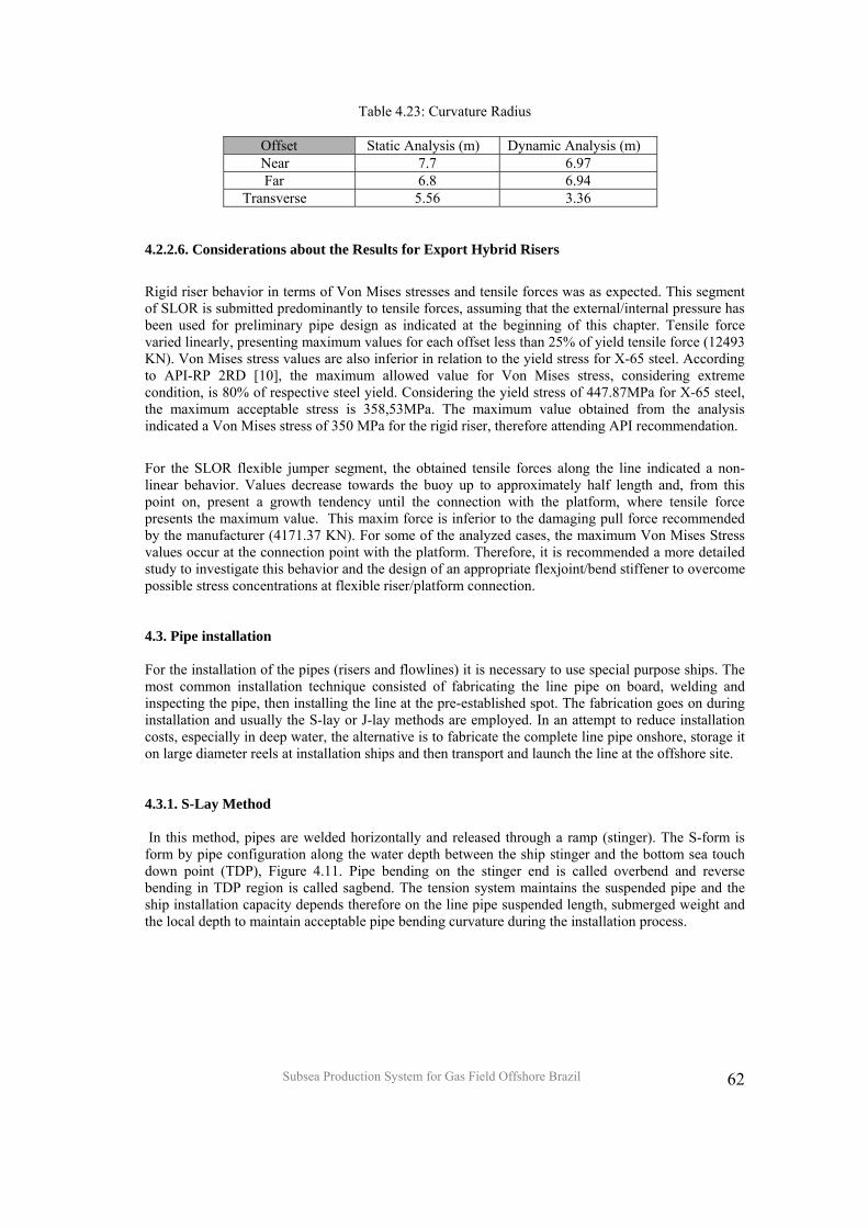
Subsea Production System for Gas Field Offshore Brazil
62
Table 4.23: Curvature Radius
Offset Static Analysis (m) Dynamic Analysis (m) Near 7.7 6.97 Far 6.8 6.94 Transverse 5.56 3.36
4.2.2.6. Considerations about the Results for Export Hybrid Risers
Rigid riser behavior in terms of Von Mises stresses and tensile forces was as expected. This segment of SLOR is submitted predominantly to tensile forces, assuming that the external/internal pressure has been used for preliminary pipe design as indicated at the beginning of this chapter. Tensile force varied linearly, presenting maximum values for each offset less than 25% of yield tensile force (12493 KN). Von Mises stress values are also inferior in relation to the yield stress for X-65 steel. According to API-RP 2RD [10], the maximum allowed value for Von Mises stress, considering extreme condition, is 80% of respective steel yield. Considering the yield stress of 447.87MPa for X-65 steel, the maximum acceptable stress is 358,53MPa. The maximum value obtained from the analysis indicated a Von Mises stress of 350 MPa for the rigid riser, therefore attending API recommendation.
For the SLOR flexible jumper segment, the obtained tensile forces along the line indicated a non-linear behavior. Values decrease towards the buoy up to approximately half length and, from this point on, present a growth tendency until the connection with the platform, where tensile force presents the maximum value. This maxim force is inferior to the damaging pull force recommended by the manufacturer (4171.37 KN). For some of the analyzed cases, the maximum Von Mises Stress values occur at the connection point with the platform. Therefore, it is recommended a more detailed study to investigate this behavior and the design of an appropriate flexjoint/bend stiffener to overcome possible stress concentrations at flexible riser/platform connection. 4.3. Pipe installation For the installation of the pipes (risers and flowlines) it is necessary to use special purpose ships. The most common installation technique consisted of fabricating the line pipe on board, welding and inspecting the pipe, then installing the line at the pre-established spot. The fabrication goes on during installation and usually the S-lay or J-lay methods are employed. In an attempt to reduce installation costs, especially in deep water, the alternative is to fabricate the complete line pipe onshore, storage it on large diameter reels at installation ships and then transport and launch the line at the offshore site. 4.3.1. S-Lay Method In this method, pipes are welded horizontally and released through a ramp (stinger). The S-form is form by pipe configuration along the water depth between the ship stinger and the bottom sea touch down point (TDP), Figure 4.11. Pipe bending on the stinger end is called overbend and reverse bending in TDP region is called sagbend. The tension system maintains the suspended pipe and the ship installation capacity depends therefore on the line pipe suspended length, submerged weight and the local depth to maintain acceptable pipe bending curvature during the installation process.
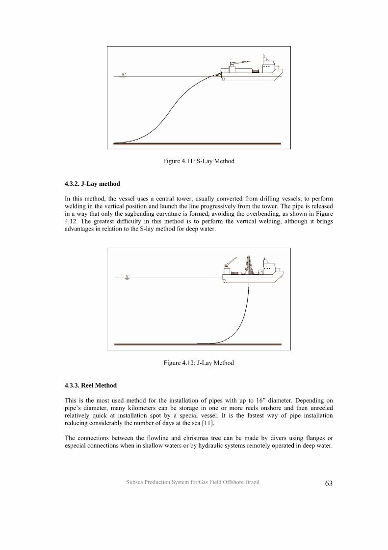
Subsea Production System for Gas Field Offshore Brazil
63
Figure 4.11: S-Lay Method
4.3.2. J-Lay method In this method, the vessel uses a central tower, usually converted from drilling vessels, to perform welding in the vertical position and launch the line progressively from the tower. The pipe is released in a way that only the sagbending curvature is formed, avoiding the overbending, as shown in Figure 4.12. The greatest difficulty in this method is to perform the vertical welding, although it brings advantages in relation to the S-lay method for deep water.
Figure 4.12: J-Lay Method 4.3.3. Reel Method This is the most used method for the installation of pipes with up to 16” diameter. Depending on pipe’s diameter, many kilometers can be storage in one or more reels onshore and then unreeled relatively quick at installation spot by a special vessel. It is the fastest way of pipe installation reducing considerably the number of days at the sea [11]. The connections between the flowline and christmas tree can be made by divers using flanges or especial connections when in shallow waters or by hydraulic systems remotely operated in deep water.

Subsea Production System for Gas Field Offshore Brazil
64
Pipes can be fully built onshore, becoming much easier the welding and inspection activities. However, pipes will be submitted to few bending cycles, which should be analyzed in a more elaborated and careful design project in order to avoid future operational problems. Once pipes are wounded on the reel, they are rectified afterwards to compensate plastic deformations. Reeling and unreeling operations may increase pipe ovality and magnify possible weld defects, therefore reducing ultimate strength and fatigue life, respectively. Installation process for the Reel method is shown in Figure 4.13.
Figure 4.13: Reel Method 4.3.4. Definition of the Installation Method For defining installation method to be used, cost and especially frequent use in national offshore activities were taken into account. For flexible risers the reel method was chosen due to its time and cost advantages in comparison to other methods. For rigid pipes due to restriction for diameters above 16", this method was not considered. Thus, the J-lay method, broadly used in Campos Basin, was selected as the best option. 4.4 Pipe Maintenance - Inspection and Cleaning Pipelines need especial planning for maintenance, in particular cleaning and inspection techniques to assure both equipment integrity and optimal flow. Recently, there has been an increase of instrumented pig passages to measure wall thickness along the pipe and identify points with reduced thickness, caused by local corrosive process. Pigs aimed at removing hydrates are more related to flow assurance. The pigs resemble to a cylinder of diameter slightly inferior to that of the pipeline and go throughout the line, removing substances accumulated on the walls. The conventional ones just clean; the intelligent ones, instrumented, make a diagnosis of the pipeline. The intelligent pigs carry a cylindrical vessel with computers and sensors to measure the pipe wall thickness and indicate corrosion and dent points. Figure 4.14 display a picture of a pig prototype, being prepared for tests in a pipeline closed loop, at PETROBRAS Research Center.
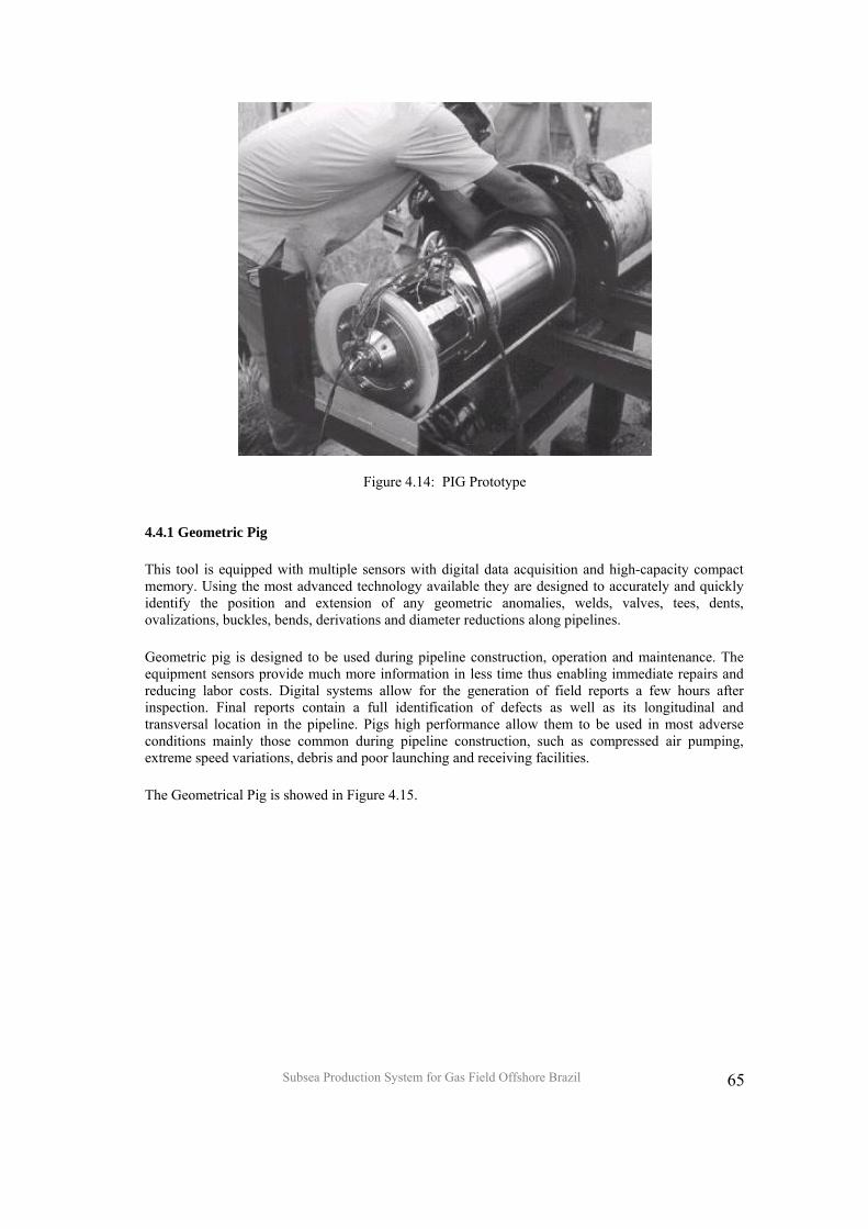
Subsea Production System for Gas Field Offshore Brazil
65
Figure 4.14: PIG Prototype
4.4.1 Geometric Pig
This tool is equipped with multiple sensors with digital data acquisition and high-capacity compact memory. Using the most advanced technology available they are designed to accurately and quickly identify the position and extension of any geometric anomalies, welds, valves, tees, dents, ovalizations, buckles, bends, derivations and diameter reductions along pipelines.
Geometric pig is designed to be used during pipeline construction, operation and maintenance. The equipment sensors provide much more information in less time thus enabling immediate repairs and reducing labor costs. Digital systems allow for the generation of field reports a few hours after inspection. Final reports contain a full identification of defects as well as its longitudinal and transversal location in the pipeline. Pigs high performance allow them to be used in most adverse conditions mainly those common during pipeline construction, such as compressed air pumping, extreme speed variations, debris and poor launching and receiving facilities.
The Geometrical Pig is showed in Figure 4.15.
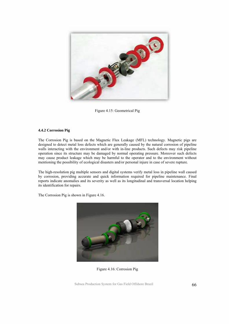
Subsea Production System for Gas Field Offshore Brazil
66
Figure 4.15: Geometrical Pig
4.4.2 Corrosion Pig
The Corrosion Pig is based on the Magnetic Flux Leakage (MFL) technology. Magnetic pigs are designed to detect metal loss defects which are generally caused by the natural corrosion of pipeline walls interacting with the environment and/or with in-line products. Such defects may risk pipeline operation since its structure may be damaged by normal operating pressure. Moreover such defects may cause product leakage which may be harmful to the operator and to the environment without mentioning the possibility of ecological disasters and/or personal injure in case of severe rupture.
The high-resolution pig multiple sensors and digital systems verify metal loss in pipeline wall caused by corrosion, providing accurate and quick information required for pipeline maintenance. Final reports indicate anomalies and its severity as well as its longitudinal and transversal location helping its identification for repairs.
The Corrosion Pig is shown in Figure 4.16.
Figure 4.16: Corrosion Pig
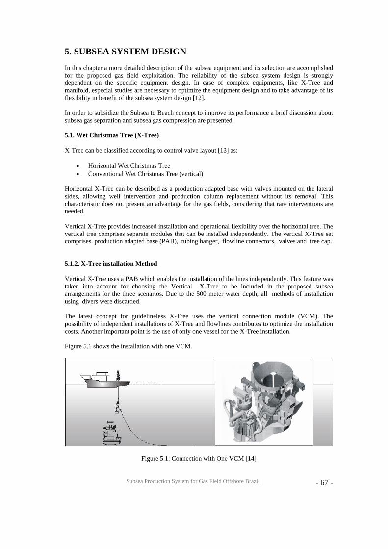
Subsea Production System for Gas Field Offshore Brazil
- 67 -
5. SUBSEA SYSTEM DESIGN In this chapter a more detailed description of the subsea equipment and its selection are accomplished for the proposed gas field exploitation. The reliability of the subsea system design is strongly dependent on the specific equipment design. In case of complex equipments, like X-Tree and manifold, especial studies are necessary to optimize the equipment design and to take advantage of its flexibility in benefit of the subsea system design [12]. In order to subsidize the Subsea to Beach concept to improve its performance a brief discussion about subsea gas separation and subsea gas compression are presented. 5.1. Wet Christmas Tree (X-Tree) X-Tree can be classified according to control valve layout [13] as:
• Horizontal Wet Christmas Tree • Conventional Wet Christmas Tree (vertical)
Horizontal X-Tree can be described as a production adapted base with valves mounted on the lateral sides, allowing well intervention and production column replacement without its removal. This characteristic does not present an advantage for the gas fields, considering that rare interventions are needed. Vertical X-Tree provides increased installation and operational flexibility over the horizontal tree. The vertical tree comprises separate modules that can be installed independently. The vertical X-Tree set comprises production adapted base (PAB), tubing hanger, flowline connectors, valves and tree cap. 5.1.2. X-Tree installation Method Vertical X-Tree uses a PAB which enables the installation of the lines independently. This feature was taken into account for choosing the Vertical X-Tree to be included in the proposed subsea arrangements for the three scenarios. Due to the 500 meter water depth, all methods of installation using divers were discarded. The latest concept for guidelineless X-Tree uses the vertical connection module (VCM). The possibility of independent installations of X-Tree and flowlines contributes to optimize the installation costs. Another important point is the use of only one vessel for the X-Tree installation. Figure 5.1 shows the installation with one VCM.
Figure 5.1: Connection with One VCM [14]
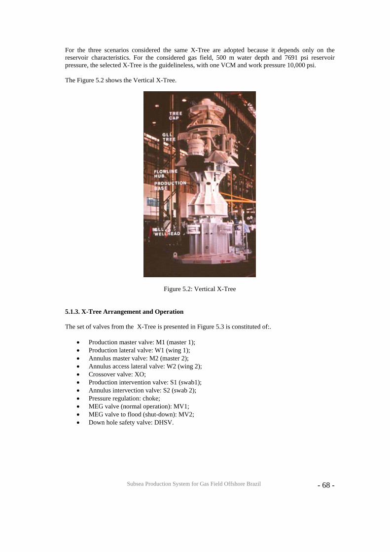
Subsea Production System for Gas Field Offshore Brazil
- 68 -
For the three scenarios considered the same X-Tree are adopted because it depends only on the reservoir characteristics. For the considered gas field, 500 m water depth and 7691 psi reservoir pressure, the selected X-Tree is the guidelineless, with one VCM and work pressure 10,000 psi. The Figure 5.2 shows the Vertical X-Tree.
Figure 5.2: Vertical X-Tree
5.1.3. X-Tree Arrangement and Operation The set of valves from the X-Tree is presented in Figure 5.3 is constituted of:.
• Production master valve: M1 (master 1); • Production lateral valve: W1 (wing 1); • Annulus master valve: M2 (master 2); • Annulus access lateral valve: W2 (wing 2); • Crossover valve: XO; • Production intervention valve: S1 (swab1); • Annulus intervection valve: S2 (swab 2); • Pressure regulation: choke; • MEG valve (normal operation): MV1; • MEG valve to flood (shut-down): MV2; • Down hole safety valve: DHSV.
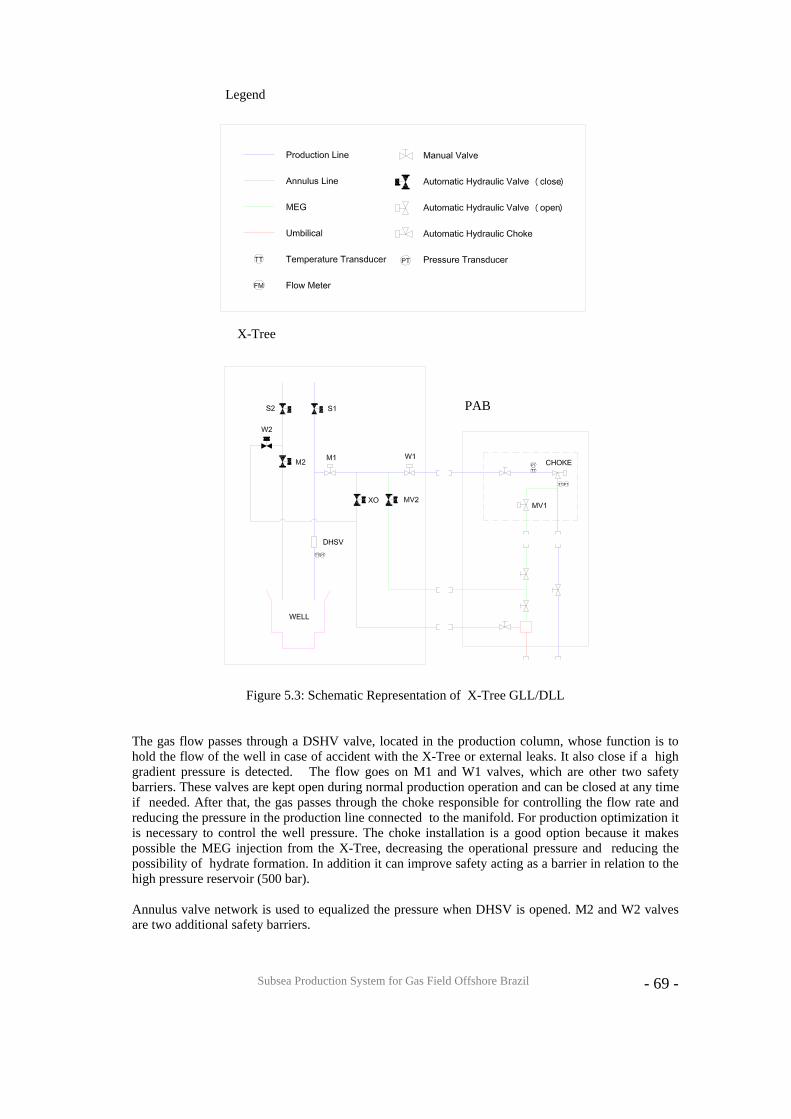
Subsea Production System for Gas Field Offshore Brazil
- 69 -
Figure 5.3: Schematic Representation of X-Tree GLL/DLL The gas flow passes through a DSHV valve, located in the production column, whose function is to hold the flow of the well in case of accident with the X-Tree or external leaks. It also close if a high gradient pressure is detected. The flow goes on M1 and W1 valves, which are other two safety barriers. These valves are kept open during normal production operation and can be closed at any time if needed. After that, the gas passes through the choke responsible for controlling the flow rate and reducing the pressure in the production line connected to the manifold. For production optimization it is necessary to control the well pressure. The choke installation is a good option because it makes possible the MEG injection from the X-Tree, decreasing the operational pressure and reducing the possibility of hydrate formation. In addition it can improve safety acting as a barrier in relation to the high pressure reservoir (500 bar). Annulus valve network is used to equalized the pressure when DHSV is opened. M2 and W2 valves are two additional safety barriers.
X-Tree
Legend
PAB
Subsea Production System for Gas Field Offshore Brazil
- 70 -
The Crossover valve is interconnected between the annulus line and the production line, being used, for example, to overcome an obstruction caused by hydrate formation. MEG network is used to inject this hydrate inhibitor. During the normal operation of the system, the MEG is injected right after the Choke through a MV1 valve, where the line pressure is smaller. Another way of doing it, is to inject through MV2 valve, usually to flood the X-Tree lines during shut down. Finally, S1 and S2 valves, located in the production and annulus lines respectively. These are intervention valves which are kept closed, being opened only when an intervention in the well is necessary. 5.1.4. Description of selected X-Tree Components 5.1.4.1. Choke Chokes are used to obtain flow and pressure control aiming at optimizing production and safety. The performance principle is based on the pressure drop by choking the section. 5.1.4.2. Base for the Flowlines This equipment supports the flowlines and control lines, leveling them in relation to the Xmas Tree. 5.1.4.3. Tubing Hanger It is responsible for the interface between the production tubing and the X-Tree. It supports the weight of the production tubing and it is anchored and locked at the production adapted base. It has also the function of sealing the annulus formed between the well coating and the production tubing. 5.1.4.4. Vertical Connection Module (VCM) The vertical connection module (VCM) has a similar function as the MLF (mandril line flow) used in CVD. The BAP optimizes the intervention resources because the X-tree installation can be performed by a drill barge and pipes and umbilicals by independent installation vessel. 5.1.5.5. Tree Cap Tree cap makes the interconnection between the stationary production unit or onshore terminal and the X-tree functions. As it is an important control equipment, it was decided to use a recoverable tree cap for easy maintenance. 5.2. Manifold Manifolds can be classified according to their function and way of installation. Regarding its function, in general, they can be classified as:
• Collecting Manifold – It collects the flow from several pipes into a single pipe; • Distribution Manifold – It distributes the flow from a single pipe to several pipes;
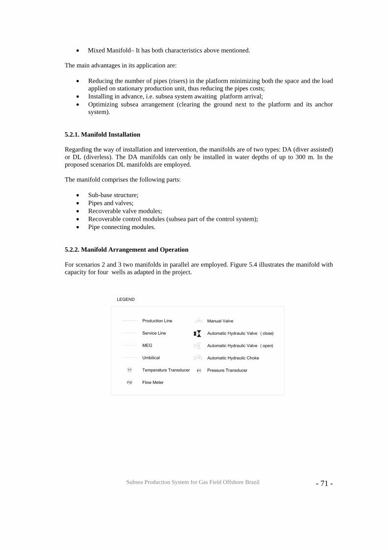
Subsea Production System for Gas Field Offshore Brazil
- 71 -
• Mixed Manifold– It has both characteristics above mentioned. The main advantages in its application are:
• Reducing the number of pipes (risers) in the platform minimizing both the space and the load applied on stationary production unit, thus reducing the pipes costs;
• Installing in advance, i.e. subsea system awaiting platform arrival; • Optimizing subsea arrangement (clearing the ground next to the platform and its anchor
system). 5.2.1. Manifold Installation Regarding the way of installation and intervention, the manifolds are of two types: DA (diver assisted) or DL (diverless). The DA manifolds can only be installed in water depths of up to 300 m. In the proposed scenarios DL manifolds are employed. The manifold comprises the following parts:
• Sub-base structure; • Pipes and valves; • Recoverable valve modules; • Recoverable control modules (subsea part of the control system); • Pipe connecting modules.
5.2.2. Manifold Arrangement and Operation For scenarios 2 and 3 two manifolds in parallel are employed. Figure 5.4 illustrates the manifold with capacity for four wells as adapted in the project.
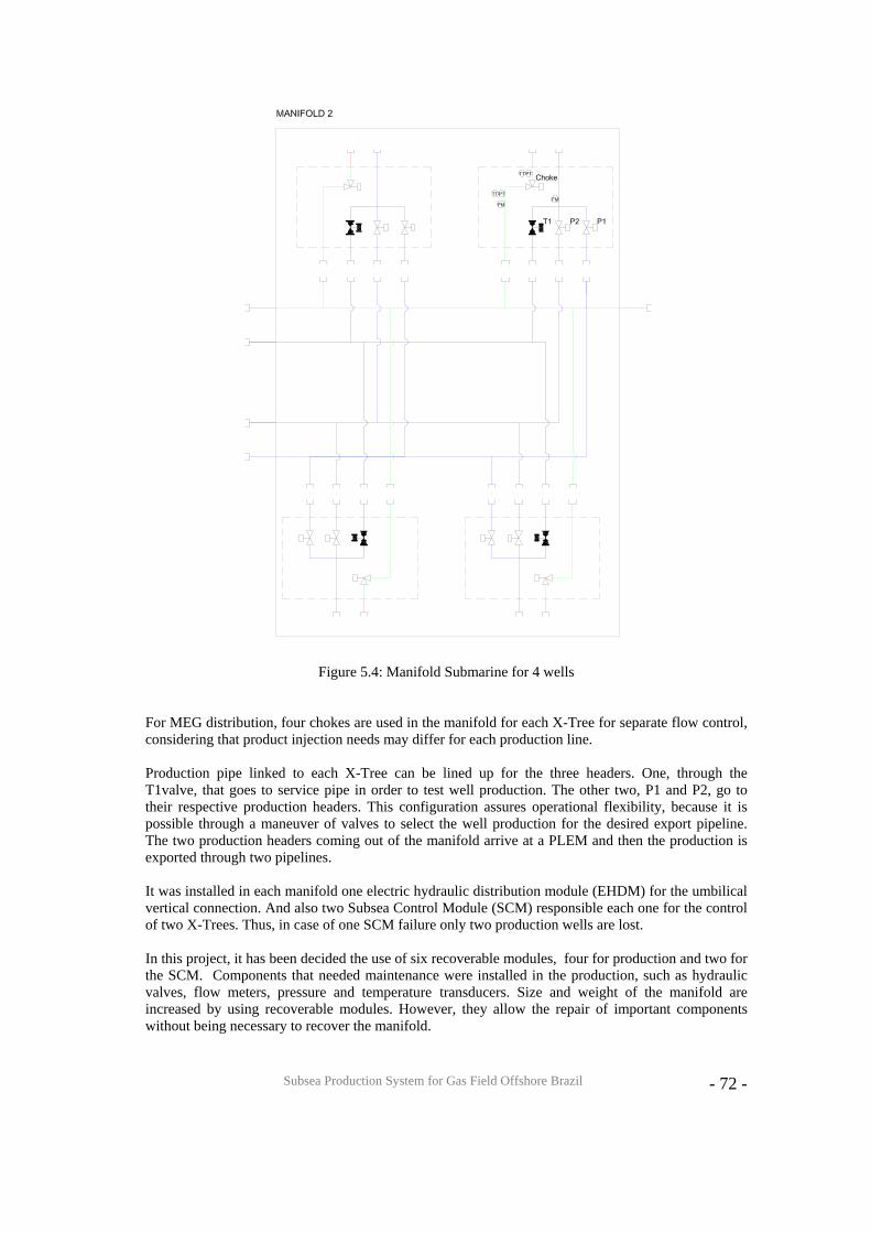
Subsea Production System for Gas Field Offshore Brazil
- 72 -
Figure 5.4: Manifold Submarine for 4 wells For MEG distribution, four chokes are used in the manifold for each X-Tree for separate flow control, considering that product injection needs may differ for each production line. Production pipe linked to each X-Tree can be lined up for the three headers. One, through the T1valve, that goes to service pipe in order to test well production. The other two, P1 and P2, go to their respective production headers. This configuration assures operational flexibility, because it is possible through a maneuver of valves to select the well production for the desired export pipeline. The two production headers coming out of the manifold arrive at a PLEM and then the production is exported through two pipelines. It was installed in each manifold one electric hydraulic distribution module (EHDM) for the umbilical vertical connection. And also two Subsea Control Module (SCM) responsible each one for the control of two X-Trees. Thus, in case of one SCM failure only two production wells are lost. In this project, it has been decided the use of six recoverable modules, four for production and two for the SCM. Components that needed maintenance were installed in the production, such as hydraulic valves, flow meters, pressure and temperature transducers. Size and weight of the manifold are increased by using recoverable modules. However, they allow the repair of important components without being necessary to recover the manifold.
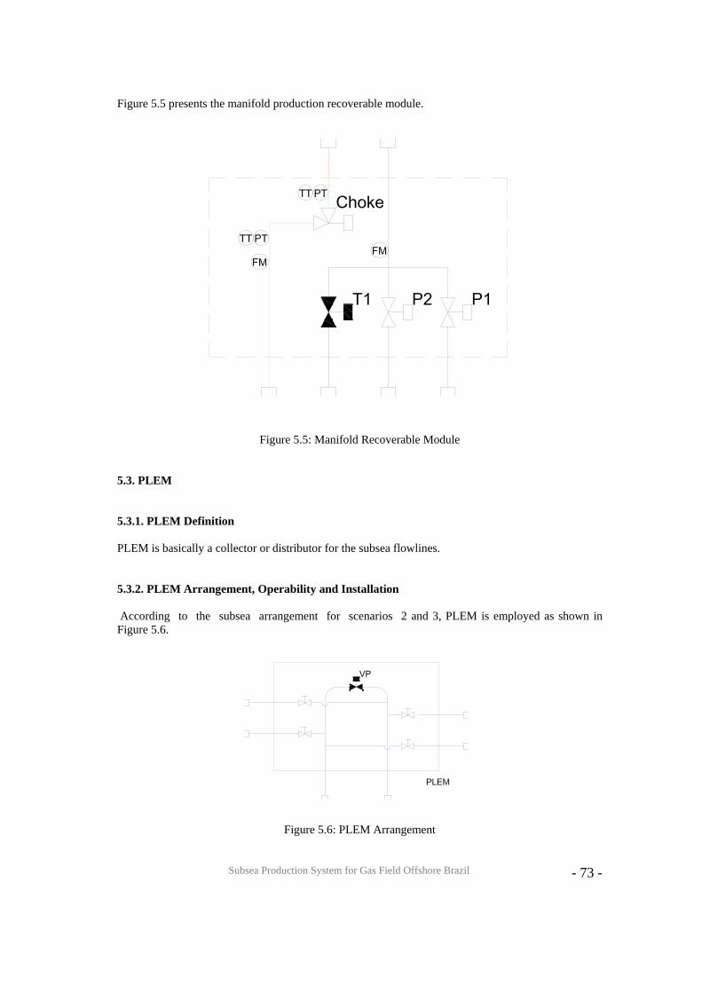
Subsea Production System for Gas Field Offshore Brazil
- 73 -
Figure 5.5 presents the manifold production recoverable module.
Figure 5.5: Manifold Recoverable Module 5.3. PLEM 5.3.1. PLEM Definition PLEM is basically a collector or distributor for the subsea flowlines. 5.3.2. PLEM Arrangement, Operability and Installation According to the subsea arrangement for scenarios 2 and 3, PLEM is employed as shown in Figure 5.6.
Figure 5.6: PLEM Arrangement
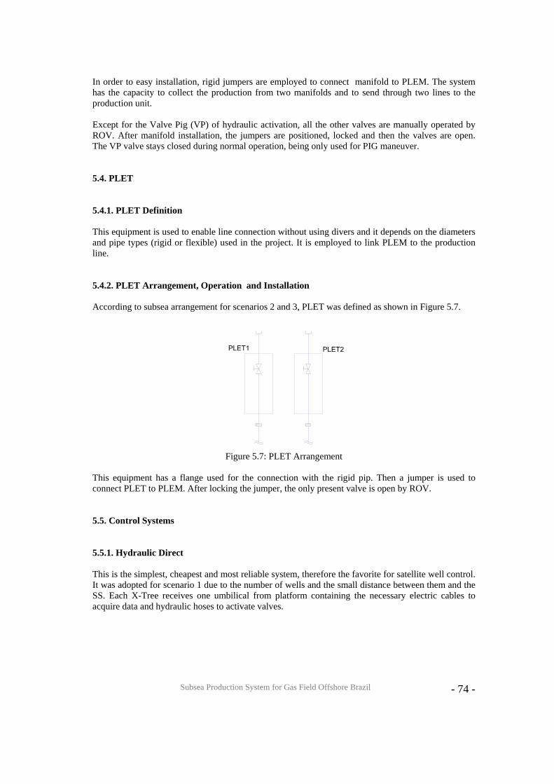
Subsea Production System for Gas Field Offshore Brazil
- 74 -
In order to easy installation, rigid jumpers are employed to connect manifold to PLEM. The system has the capacity to collect the production from two manifolds and to send through two lines to the production unit. Except for the Valve Pig (VP) of hydraulic activation, all the other valves are manually operated by ROV. After manifold installation, the jumpers are positioned, locked and then the valves are open. The VP valve stays closed during normal operation, being only used for PIG maneuver. 5.4. PLET 5.4.1. PLET Definition This equipment is used to enable line connection without using divers and it depends on the diameters and pipe types (rigid or flexible) used in the project. It is employed to link PLEM to the production line. 5.4.2. PLET Arrangement, Operation and Installation According to subsea arrangement for scenarios 2 and 3, PLET was defined as shown in Figure 5.7.
Figure 5.7: PLET Arrangement
This equipment has a flange used for the connection with the rigid pip. Then a jumper is used to connect PLET to PLEM. After locking the jumper, the only present valve is open by ROV. 5.5. Control Systems 5.5.1. Hydraulic Direct This is the simplest, cheapest and most reliable system, therefore the favorite for satellite well control. It was adopted for scenario 1 due to the number of wells and the small distance between them and the SS. Each X-Tree receives one umbilical from platform containing the necessary electric cables to acquire data and hydraulic hoses to activate valves.
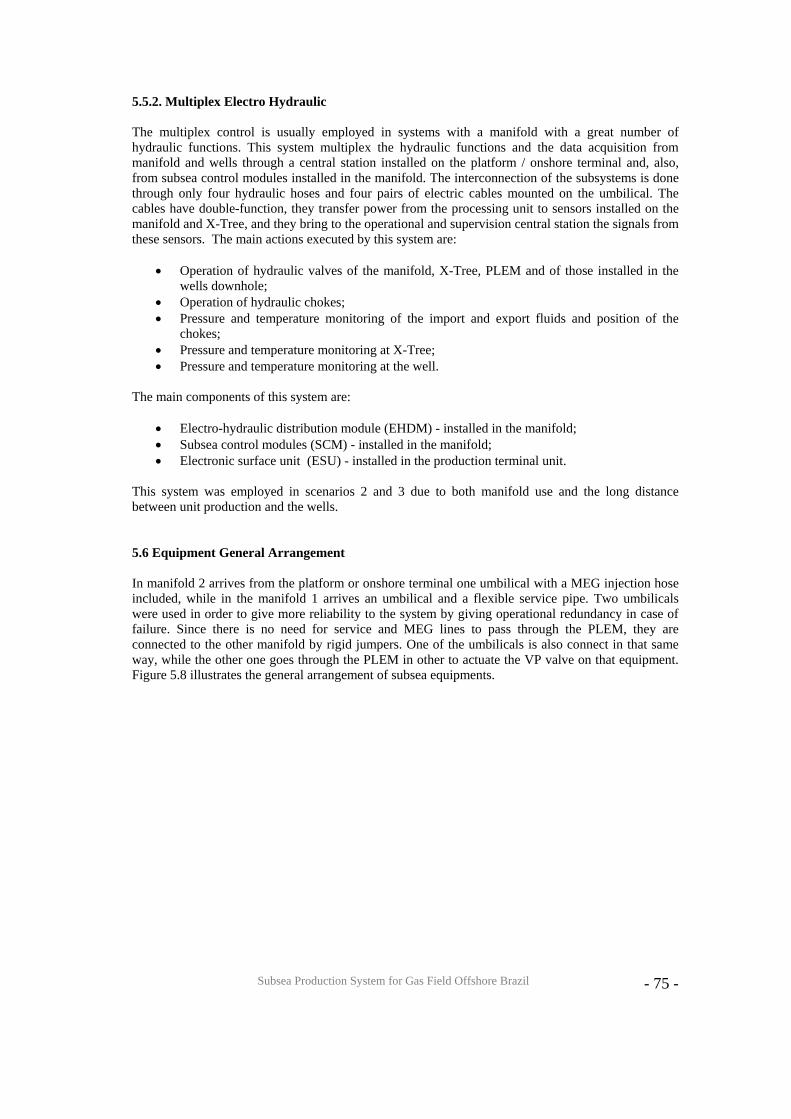
Subsea Production System for Gas Field Offshore Brazil
- 75 -
5.5.2. Multiplex Electro Hydraulic The multiplex control is usually employed in systems with a manifold with a great number of hydraulic functions. This system multiplex the hydraulic functions and the data acquisition from manifold and wells through a central station installed on the platform / onshore terminal and, also, from subsea control modules installed in the manifold. The interconnection of the subsystems is done through only four hydraulic hoses and four pairs of electric cables mounted on the umbilical. The cables have double-function, they transfer power from the processing unit to sensors installed on the manifold and X-Tree, and they bring to the operational and supervision central station the signals from these sensors. The main actions executed by this system are:
• Operation of hydraulic valves of the manifold, X-Tree, PLEM and of those installed in the wells downhole;
• Operation of hydraulic chokes; • Pressure and temperature monitoring of the import and export fluids and position of the
chokes; • Pressure and temperature monitoring at X-Tree; • Pressure and temperature monitoring at the well.
The main components of this system are:
• Electro-hydraulic distribution module (EHDM) - installed in the manifold; • Subsea control modules (SCM) - installed in the manifold; • Electronic surface unit (ESU) - installed in the production terminal unit.
This system was employed in scenarios 2 and 3 due to both manifold use and the long distance between unit production and the wells. 5.6 Equipment General Arrangement In manifold 2 arrives from the platform or onshore terminal one umbilical with a MEG injection hose included, while in the manifold 1 arrives an umbilical and a flexible service pipe. Two umbilicals were used in order to give more reliability to the system by giving operational redundancy in case of failure. Since there is no need for service and MEG lines to pass through the PLEM, they are connected to the other manifold by rigid jumpers. One of the umbilicals is also connect in that same way, while the other one goes through the PLEM in other to actuate the VP valve on that equipment. Figure 5.8 illustrates the general arrangement of subsea equipments.
Subsea Production System for Gas Field Offshore Brazil
76
Figure 5.8: Equipment General Arrangement
Subsea Production System for Gas Field Offshore Brazil
- 77 -
5.7. Subsea Compression and Separation Reservoir pressure drops throughout the field production lifetime. This will impact production rate and profitability, especially for the Subsea to Beach case due to the 160km of production pipelines. Because of that, the use of a subsea compressor was considered. Before compression can be made, it is necessary to separate the water associated with de gas and the condensate. For that, it is essential to also install a subsea separator. This system is focused on the following process [15]:
• Separation of water, gas and condensate; • Re-injection of the separated water into the reservoir; • Compression of the dehydrated gas; • Mixture the compressed gas with the condensate; • Export the gas and condensate mixture.
The installation of this two equipments, subsea separator and subsea compressor, would solve the pressure drop problem, conferring profitability and a series of advantages to the Subsea to Beach scenario:
• Draw out of the field production; • Better field management. The separation of water would help on hydrate prevention; • Reduced environment impact. The separated water can be re-injected into the reservoir.
5.7.1. Subsea Separation The economic potential of subsea separation has been known for some time. Yet, while there are a substantial number of subsea pump systems in operation, there are only two subsea separation stations installed. One is the Troll Pilot for water separation and reinjection, operated by Norsk Hydro in the North Sea. The second installation is the VASP system for gas-liquid separation and boosting operated by Petrobras in Brazil. There are interrelated reasons why the development of subsea separation applications has lagged. First, some components of such a system would have to be newly designed and qualified. Second, a system incorporating new technology carries a higher potential risk. In addition to undemonstrated performance, both durability and ease of maintenance would need to be addressed to reduce the unknown aspect of the risk. Accordingly, plans for any new design must include qualification to minimize the risk of a new technology. 5.7.2. Subsea Compression The subsea compression equipment is the biggest challenge for the proposed implementation. Because it is a totally new technology, the potential risk is high, as said before. Accordingly to the site gepower.com, GE and KOP are working to develop a 12.5 MW compression unit with market expectation for 2008, so the possibility on using such equipment is set to 2020, after approximately 10 years research. 5.7.3. Process Description All production is directed to de subsea separator, which will be responsible for separating the water, the condensate and the gas. The gas is then compressed and put together with the condensate. At this point the mixture is exported through production pipelines to the terminal. The separated water is then re-injected in the field.

Subsea Production System for Gas Field Offshore Brazil
- 78 -
For system optimization, it is better to position the equipments as near to the field as possible. For scenario 3 the appropriated place is near the PLEM.
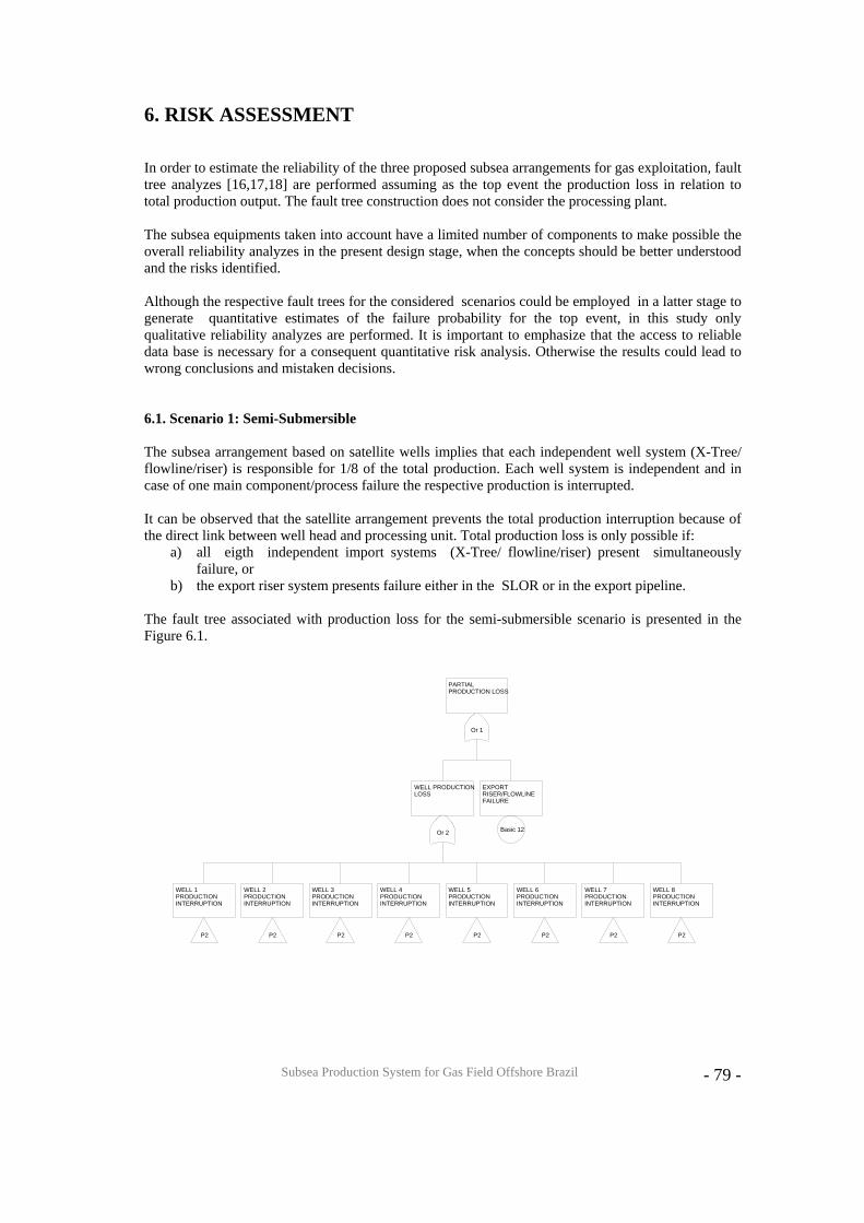
Subsea Production System for Gas Field Offshore Brazil
- 79 -
6. RISK ASSESSMENT In order to estimate the reliability of the three proposed subsea arrangements for gas exploitation, fault tree analyzes [16,17,18] are performed assuming as the top event the production loss in relation to total production output. The fault tree construction does not consider the processing plant. The subsea equipments taken into account have a limited number of components to make possible the overall reliability analyzes in the present design stage, when the concepts should be better understood and the risks identified. Although the respective fault trees for the considered scenarios could be employed in a latter stage to generate quantitative estimates of the failure probability for the top event, in this study only qualitative reliability analyzes are performed. It is important to emphasize that the access to reliable data base is necessary for a consequent quantitative risk analysis. Otherwise the results could lead to wrong conclusions and mistaken decisions. 6.1. Scenario 1: Semi-Submersible The subsea arrangement based on satellite wells implies that each independent well system (X-Tree/ flowline/riser) is responsible for 1/8 of the total production. Each well system is independent and in case of one main component/process failure the respective production is interrupted. It can be observed that the satellite arrangement prevents the total production interruption because of the direct link between well head and processing unit. Total production loss is only possible if:
a) all eigth independent import systems (X-Tree/ flowline/riser) present simultaneously failure, or
b) the export riser system presents failure either in the SLOR or in the export pipeline. The fault tree associated with production loss for the semi-submersible scenario is presented in the Figure 6.1.
cence - Not for commercial use
PARTIALPRODUCTION LOSS
Or 1
WELL PRODUCTIONLOSS
Or 2
WELL 1PRODUCTIONINTERRUPTION
P2
WELL 2PRODUCTIONINTERRUPTION
P2
WELL 3PRODUCTIONINTERRUPTION
P2
WELL 4PRODUCTIONINTERRUPTION
P2
WELL 5PRODUCTIONINTERRUPTION
P2
WELL 6PRODUCTIONINTERRUPTION
P2
WELL 7PRODUCTIONINTERRUPTION
P2
WELL 8PRODUCTIONINTERRUPTION
P2
EXPORTRISER/FLOWLINEFAILURE
Basic 12
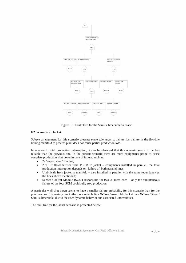
Subsea Production System for Gas Field Offshore Brazil
- 80 -
P2
WELL PRODUCTIONINTERRUPTION
Or 2
UMBILICAL FAILURE
Basic 1
X-TREE FAILURE
Or 2
AILURE IN THECONNECTIONS
Basic 6
VALVES FAILURE
Or 13
MASTER 1 FAILURE
Basic 7
WING 1 FAILURE
Basic 8
DHSV FAILURE
Basic 9
CHOKE FAILURE
Basic 10
8" FLOWLINE/RISERFAILURE
Or 15
HYDRATE BLOCK
Basic 4
STRUCTURALFAILURE
Basic 5
Figure 6.1: Fault Tree for the Semi-submersible Scenario 6.2. Scenario 2: Jacket Subsea arrangement for this scenario presents some tolerances to failure, i.e. failure in the flowline linking manifold to process plant does not cause partial production loss. In relation to total production interruption, it can be observed that this scenario seems to be less reliable than the previous one. In the present scenario there are more equipments prone to cause complete production shut down in case of failure, such as:
• 22" export riser/flowline; • 2 x 18" flowline/riser from PLEM to jacket – equipments installed in parallel, the total
production interruption depends on failure of both parallel lines; • Umbilicals from jacket to manifold – also installed in parallel with the same redundancy as
the lines above mentioned; • Subsea Control Module (SCM) responsible for two X-Trees each – only the simultaneous
failure of the four SCM could fully stop production. A particular well shut down seems to have a smaller failure probability for this scenario than for the previous one. It is mainly due to the more reliable link X-Tree / manifold / Jacket than X-Tree / Riser / Semi-submersible, due to the riser dynamic behavior and associated uncertainties. The fault tree for the jacket scenario is presented below.
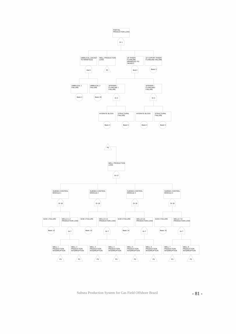
Subsea Production System for Gas Field Offshore Brazil
- 81 -
cence - Not for commercial usePARTIALPRODUCTION LOSS
Or 1
UMBILICAL (JACKETTO MANIFOLD)
And 1
UMBILICAL 1FAILURE
Basic 2
UMBILICAL 2FAILURE
Basic 20
WELL PRODUCTIONLOSS
P2
18" RISER/FLOWLINE(MANIFOLD TOJACKET)
End 2
18"RISER /FLOWLINE 1FAILURE
Or 3
HYDRATE BLOCK
Basic 4
STRUCTURALFAILURE
Basic 5
18"RISER /FLOWLINE2FAILURE
Or 3
HYDRATE BLOCK
Basic 4
STRUCTURALFAILURE
Basic 5
22" EXPORT RISER/FLOWLINE FAILURE
Basic 3
P2
WELL PRODUCTIONLOSS
Or 17
SUBSEA CONTROLMODULE 1
Or 18
SCM 1 FAILURE
Basic 12
WELLS 1-2PRODUCTION LOSS
Or 7
WELL 1PRODUCTIONINTERRUPTION
P3
WELL 2PRODUCTIONINTERRUPTION
P3
SUBSEA CONTROLMODULE 2
Or 18
SCM 2 FAILURE
Basic 13
WELLS 3-4PRODUCTION LOSS
Or 7
WELL 3PRODUCTIONINTERRUPTION
P3
WELL 4PRODUCTIONINTERRUPTION
P3
SUBSEA CONTROLMODULE 3
Or 18
SCM 3 FAILURE
Basic 14
WELLS 5-6PRODUCTION LOSS
Or 7
WELL 5PRODUCTIONINTERRUPTION
P3
WELL 6PRODUCTIONINTERRUPTION
P3
SUBSEA CONTROLMODULE 4
Or 18
SCM 4 FAILURE
Basic 15
WELLS 7-8PRODUCTION LOSS
Or 7
WELL 7PRODUCTIONINTERRUPTION
P3
WELL 8PRODUCTIONINTERRUPTION
P3
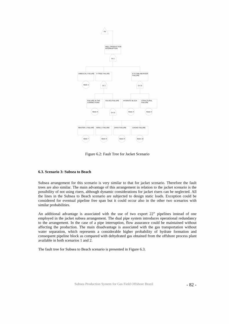
Subsea Production System for Gas Field Offshore Brazil
- 82 -
P3
WELL PRODUCTIONINTERRUPTION
Or 2
UMBILICAL FAILURE
Basic 1
X-TREE FAILURE
Or 2
FAILURE IN THECONNECTIONS
Basic 6
VALVES FAILURE
Or 13
MASTER 1 FAILURE
Basic 7
WING 1 FAILURE
Basic 8
DHSV FAILURE
Basic 9
CHOKE FAILURE
Basic 10
8" FLOWLINE/RISERFAILURE
Or 15
HYDRATE BLOCK
Basic 4
STRUCTURALFAILURE
Basic 5
Figure 6.2: Fault Tree for Jacket Scenario
6.3. Scenario 3: Subsea to Beach
Subsea arrangement for this scenario is very similar to that for jacket scenario. Therefore the fault trees are also similar. The main advantage of this arrangement in relation to the jacket scenario is the possibility of not using risers, although dynamic considerations for jacket risers can be neglected. All the lines in the Subsea to Beach scenario are subjected to design static loads. Exception could be considered for eventual pipeline free span but it could occur also in the other two scenarios with similar probabilities. An additional advantage is associated with the use of two export 22” pipelines instead of one employed in the jacket subsea arrangement. The dual pipe system introduces operational redundancy to the arrangement. In the case of a pipe interruption, flow assurance could be maintained without affecting the production. The main disadvantage is associated with the gas transportation without water separation, which represents a considerable higher probability of hydrate formation and consequent pipeline block as compared with dehydrated gas obtained from the offshore process plant available in both scenarios 1 and 2. The fault tree for Subsea to Beach scenario is presented in Figure 6.3.
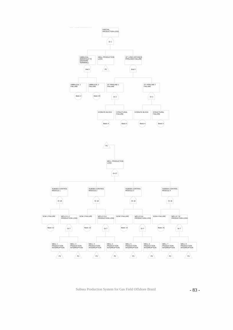
Subsea Production System for Gas Field Offshore Brazil
- 83 -
cence - Not for commercial usePARTIALPRODUCTION LOSS
Or 1
UMBILICAL(MANIFOLD TOONSHORETERMINAL)
And 1
UMBILICAL 1FAILURE
Basic 2
UMBILICAL 2FAILURE
Basic 20
WELL PRODUCTIONLOSS
P2
22" LONG DISTANCEPIPELINES FAILURE
End 2
22" PIPELINE 1FAILURE
Or 3
hYDRATE BLOCK
Basic 4
STRUCTURALFAILURE
Basic 5
22" PIPELINE 2FAILURE
Or 3
hYDRATE BLOCK
Basic 4
STRUCTURALFAILURE
Basic 5
P2
WELL PRODUCTIONLOSS
Or 17
SUBSEA CONTROLMODULE 1
Or 18
SCM 1 FAILURE
Basic 12
WELLS 1-2PRODUCTION LOSS
Or 7
WELL 1PRODUCTIONINTERRUPTION
P3
WELL 2PRODUCTIONINTERRUPTION
P3
SUBSEA CONTROLMODULE 2
Or 18
SCM 2 FAILURE
Basic 13
WELLS 3-4PRODUCTION LOSS
Or 7
WELL 3PRODUCTIONINTERRUPTION
P3
WELL 4PRODUCTIONINTERRUPTION
P3
SUBSEA CONTROLMODULE 3
Or 18
SCM 3 FAILURE
Basic 14
WELLS 5-6PRODUCTION LOSS
Or 7
WELL 5PRODUCTIONINTERRUPTION
P3
WELL 6PRODUCTIONINTERRUPTION
P3
SUBSEA CONTROLMODULE 4
Or 18
SCM 4 FAILURE
Basic 15
WELLS 7-8PRODUCTION LOSS
Or 7
WELL 7PRODUCTIONINTERRUPTION
P3
WELL 8PRODUCTIONINTERRUPTION
P3
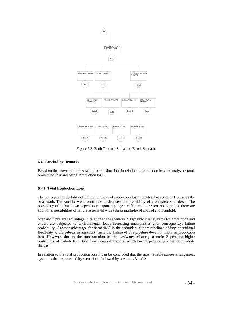
Subsea Production System for Gas Field Offshore Brazil
- 84 -
P3
WELL PRODUCTIONINTERRUPTION
Or 2
UMBILICAL FAILURE
Basic 1
X-TREE FAILURE
Or 2
CONNECTIONSEMPTYING
Basic 6
VALVES FAILURE
Or 13
MASTER 1 FAILURE
Basic 7
WING 1 FAILURE
Basic 8
DHSV FAILURE
Basic 9
CHOKE FAILURE
Basic 10
8" FLOWLINE/RISERFAILURE
Or 15
hYDRATE BLOCK
Basic 4
STRUCTURALFAILURE
Basic 5
Figure 6.3: Fault Tree for Subsea to Beach Scenario
6.4. Concluding Remarks Based on the above fault trees two different situations in relation to production loss are analyzed: total production loss and partial production loss. 6.4.1. Total Production Loss The conceptual probability of failure for the total production loss indicates that scenario 1 presents the best result. The satellite wells contribute to decrease the probability of a complete shut down. The possibility of a shut down depends on export pipe system failure. For scenarios 2 and 3, there are additional possibilities of failure associated with subsea multiplexed control and manifold. Scenario 3 presents advantage in relation to the scenario 2. Dynamic riser systems for production and export are subjected to environmental loads increasing uncertainties and, consequently, failure probability. Another advantage for scenario 3 is the redundant export pipelines adding operational flexibility to the subsea arrangement, since the failure of one pipeline does not imply in production loss. However, due to the transportation of the gas/water mixture, scenario 3 presents higher probability of hydrate formation than scenarios 1 and 2, which have separation process to dehydrate the gas. In relation to the total production loss it can be concluded that the most reliable subsea arrangement system is that represented by scenario 1, followed by scenarios 3 and 2.
Subsea Production System for Gas Field Offshore Brazil
- 85 -
6.4.2. Partial Production Loss The partial production loss considers only one well interruption. Analyzing the subsea arrangements and respective fault trees it can be observed that scenarios 2 and 3 are more reliable than scenario 1. As already mentioned the advantage of on-bottom import system using manifolds and electro-hydraulic multiplex control reflects on smaller failure probability if compared with the import and export dynamic risers in scenario 1. In general, it can be concluded that scenarios 2 and 3 are more reliable than scenario 1 for partial production loss. In this case it is difficult to distinguish scenarios 2 and 3. Although scenario 3 has two redundant export pipelines, the transport of water/gas mixture increases the probability of hydrate formation if compared with scenario 2, although in this scenario there is no pipeline redundancy. 6.4.3. The Best Scenario Considering that the total production loss is associated with a failure probability substantially smaller than for the partial production loss, the indication of the most reliable scenario should take into consideration small production losses during the project life cycle. The satellite wells associated with dynamic risers again put the scenario 1 as the less attractive alternative. Although equivalent in terms of partial production loss, scenario 3 is more reliable than scenario 2 for total production loss. Therefore, based on the qualitative risk assessment for production loss, the scenario 3 can be indicated as the best option for the offshore gas field considered in this project. However, the possibility of gas/water subsea separation and subsea gas compression, before export to onshore terminal, could mean an outstanding advantage for Subsea to Beach scenario in relation to both Semi-submersible and Jacket scenarios. In addition, the possibility of only one export pipeline could be considered for the Subsea to Beach scenario for dehydrated gas.
Subsea Production System for Gas Field Offshore Brazil
- 86 -
7. COSTS When determining the best subsea system design, the costs always play an important role. Profitability is one of main objectives of an investment, so the capability of generating profit is of paramount importance. The total cost when developing a subsea exploitation field is a function of several income and expense factors such as capital expenditures (CAPEX), operational expenditures (OPEX), production rate, product price, frequency of component failures and intervention vessels [19]. Because the value of a project is based on its capability to generate future cash flow, the investment alternatives can only be compared if measured at the same time. To do that, economists use a well know method called Net Present Value (NPV), which will be considered in this chapter. Cost analysis to implement each scenario and all the other costs associated with operation and maintenance aspects are treated. 7.1. Net Present Value (NPV) This method measures the present value of all future income or expense during the project’s life cycle. Projects with positive NPV values mean the investment worth more than it costs.
∑= +
+−=n
tt
t
KCF
INPV1 )1(
where I = inicial investment
tCF = cash flow at time t
K = discount rate t = time (period) 7.2. Master Schedule In order to organize the cost study, the team felt it was necessary to create a construction Master Schedule of each scenario, which helped determining the payments period for use of the NPV method. To do that, a market research was made to find out delivery and installation times for the subsea equipments, pipelines and platforms. To better resume the information that was gathered, Gantt charts were used. Marine related industries commonly use Gantt charts to organize a project by breaking down its complexity. With that in mind, the group developed each scenario Master Schedule, and assumed a bid process to take place in order to get the best combination of price and time delivery in the market. By doing this, competition was assured since the winner for each project area (platform construction, equipments and pipelines) would be the one with the best prices. Also, the delivery times would be guaranteed. The next pages show the preliminary Master Schedule in Figures 7.1, 7.2 and 7.3 respectively for scenarios 1, 2 and 3.
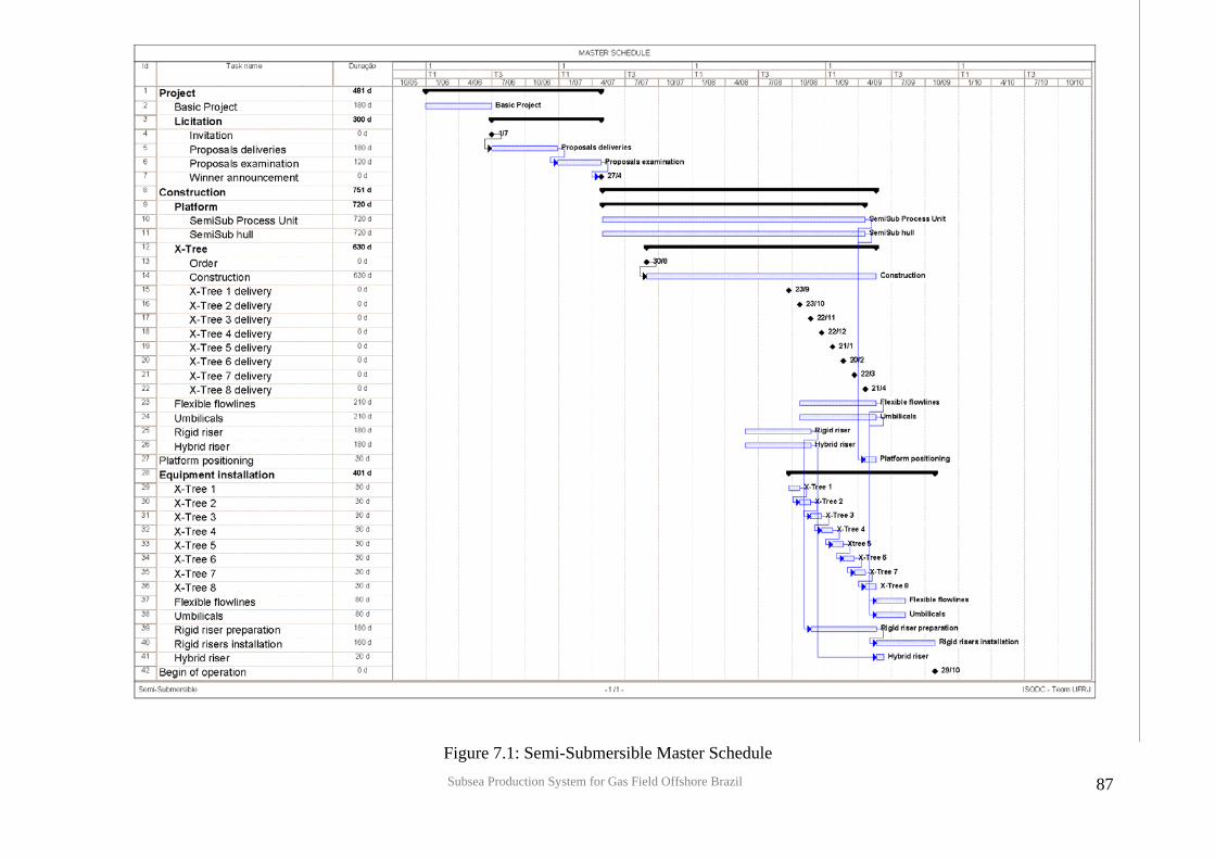
Subsea Production System for Gas Field Offshore Brazil
87
Figure 7.1: Semi-Submersible Master Schedule
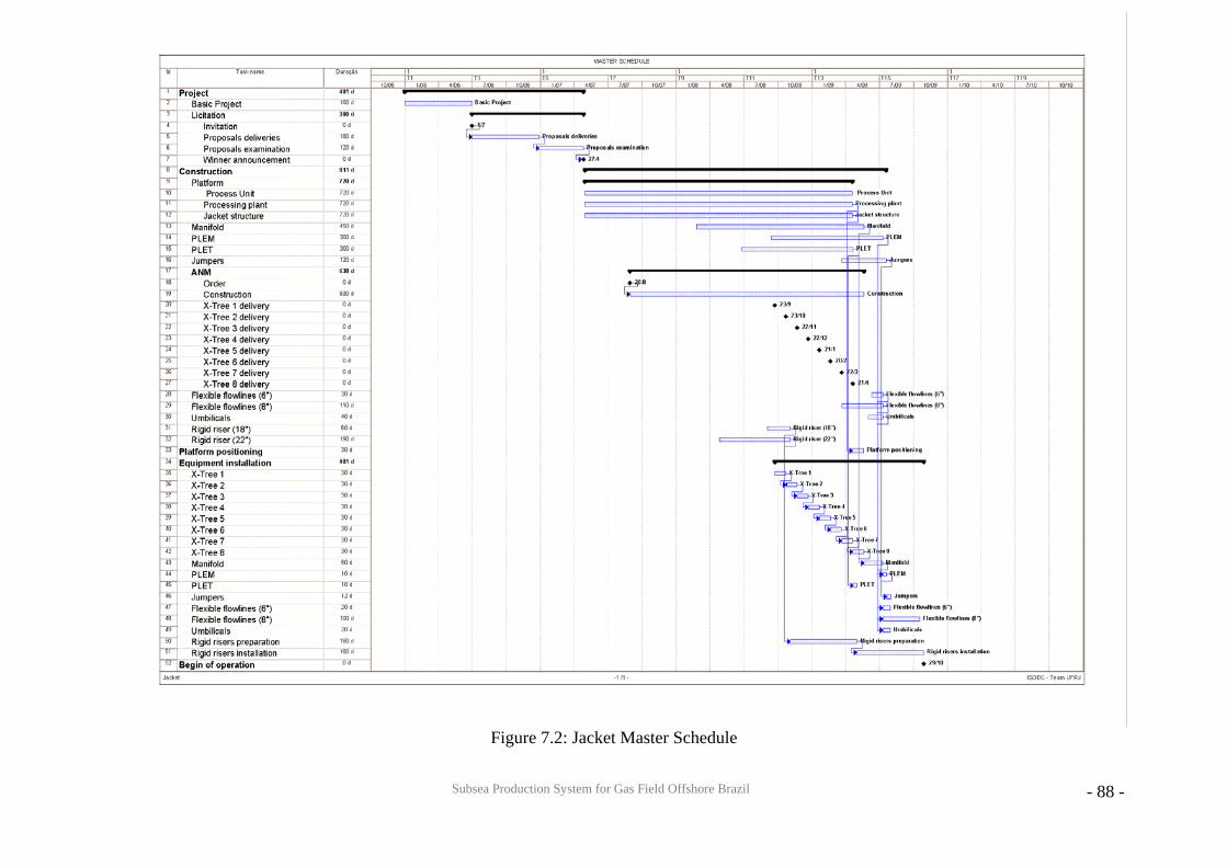
Subsea Production System for Gas Field Offshore Brazil
- 88 -
Figure 7.2: Jacket Master Schedule
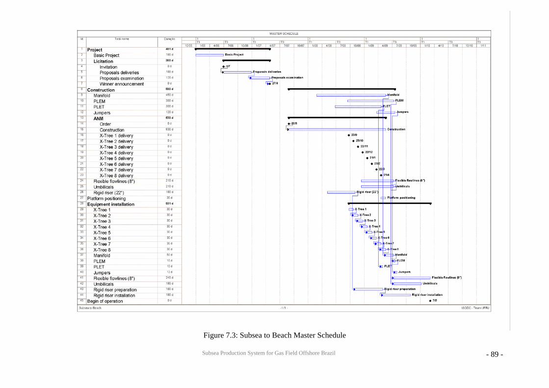
Subsea Production System for Gas Field Offshore Brazil
- 89 -
Figure 7.3: Subsea to Beach Master Schedule
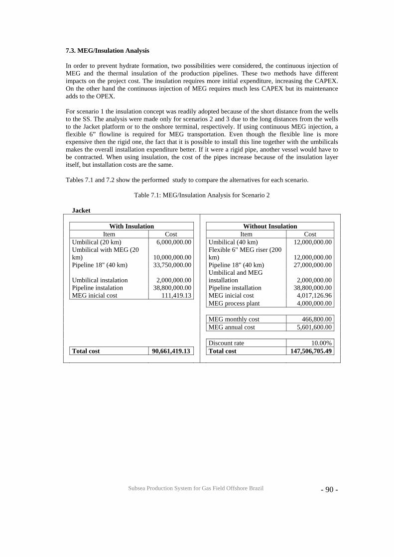
Subsea Production System for Gas Field Offshore Brazil
- 90 -
7.3. MEG/Insulation Analysis In order to prevent hydrate formation, two possibilities were considered, the continuous injection of MEG and the thermal insulation of the production pipelines. These two methods have different impacts on the project cost. The insulation requires more initial expenditure, increasing the CAPEX. On the other hand the continuous injection of MEG requires much less CAPEX but its maintenance adds to the OPEX. For scenario 1 the insulation concept was readily adopted because of the short distance from the wells to the SS. The analysis were made only for scenarios 2 and 3 due to the long distances from the wells to the Jacket platform or to the onshore terminal, respectively. If using continuous MEG injection, a flexible 6” flowline is required for MEG transportation. Even though the flexible line is more expensive then the rigid one, the fact that it is possible to install this line together with the umbilicals makes the overall installation expenditure better. If it were a rigid pipe, another vessel would have to be contracted. When using insulation, the cost of the pipes increase because of the insulation layer itself, but installation costs are the same. Tables 7.1 and 7.2 show the performed study to compare the alternatives for each scenario.
Table 7.1: MEG/Insulation Analysis for Scenario 2
Jacket With Insulation Without Insulation Item Cost Item Cost Umbilical (20 km) 6,000,000.00 Umbilical (40 km) 12,000,000.00
Umbilical with MEG (20 km) 10,000,000.00
Flexible 6" MEG riser (200 km) 12,000,000.00
Pipeline 18" (40 km) 33,750,000.00 Pipeline 18" (40 km) 27,000,000.00
Umbilical instalation 2,000,000.00 Umbilical and MEG installation 2,000,000.00
Pipeline instalation 38,800,000.00 Pipeline installation 38,800,000.00 MEG inicial cost 111,419.13 MEG inicial cost 4,017,126.96 MEG process plant 4,000,000.00 MEG monthly cost 466,800.00 MEG annual cost 5,601,600.00 Discount rate 10.00% Total cost 90,661,419.13 Total cost 147,506,705.49
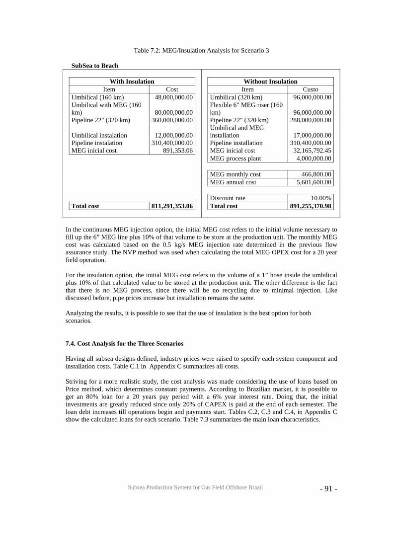
Subsea Production System for Gas Field Offshore Brazil
- 91 -
Table 7.2: MEG/Insulation Analysis for Scenario 3
SubSea to Beach With Insulation Without Insulation Item Cost Item Custo Umbilical (160 km) 48,000,000.00 Umbilical (320 km) 96,000,000.00
Umbilical with MEG (160 km) 80,000,000.00
Flexible 6" MEG riser (160 km) 96,000,000.00
Pipeline 22" (320 km) 360,000,000.00 Pipeline 22" (320 km) 288,000,000.00
Umbilical instalation 12,000,000.00 Umbilical and MEG installation 17,000,000.00
Pipeline instalation 310,400,000.00 Pipeline installation 310,400,000.00 MEG inicial cost 891,353.06 MEG inicial cost 32,165,792.45 MEG process plant 4,000,000.00 MEG monthly cost 466,800.00 MEG annual cost 5,601,600.00 Discount rate 10.00% Total cost 811,291,353.06 Total cost 891,255,370.98 In the continuous MEG injection option, the initial MEG cost refers to the initial volume necessary to fill up the 6” MEG line plus 10% of that volume to be store at the production unit. The monthly MEG cost was calculated based on the 0.5 kg/s MEG injection rate determined in the previous flow assurance study. The NVP method was used when calculating the total MEG OPEX cost for a 20 year field operation. For the insulation option, the initial MEG cost refers to the volume of a 1” hose inside the umbilical plus 10% of that calculated value to be stored at the production unit. The other difference is the fact that there is no MEG process, since there will be no recycling due to minimal injection. Like discussed before, pipe prices increase but installation remains the same. Analyzing the results, it is possible to see that the use of insulation is the best option for both scenarios. 7.4. Cost Analysis for the Three Scenarios Having all subsea designs defined, industry prices were raised to specify each system component and installation costs. Table C.1 in Appendix C summarizes all costs. Striving for a more realistic study, the cost analysis was made considering the use of loans based on Price method, which determines constant payments. According to Brazilian market, it is possible to get an 80% loan for a 20 years pay period with a 6% year interest rate. Doing that, the initial investments are greatly reduced since only 20% of CAPEX is paid at the end of each semester. The loan debt increases till operations begin and payments start. Tables C.2, C.3 and C.4, in Appendix C show the calculated loans for each scenario. Table 7.3 summarizes the main loan characteristics.
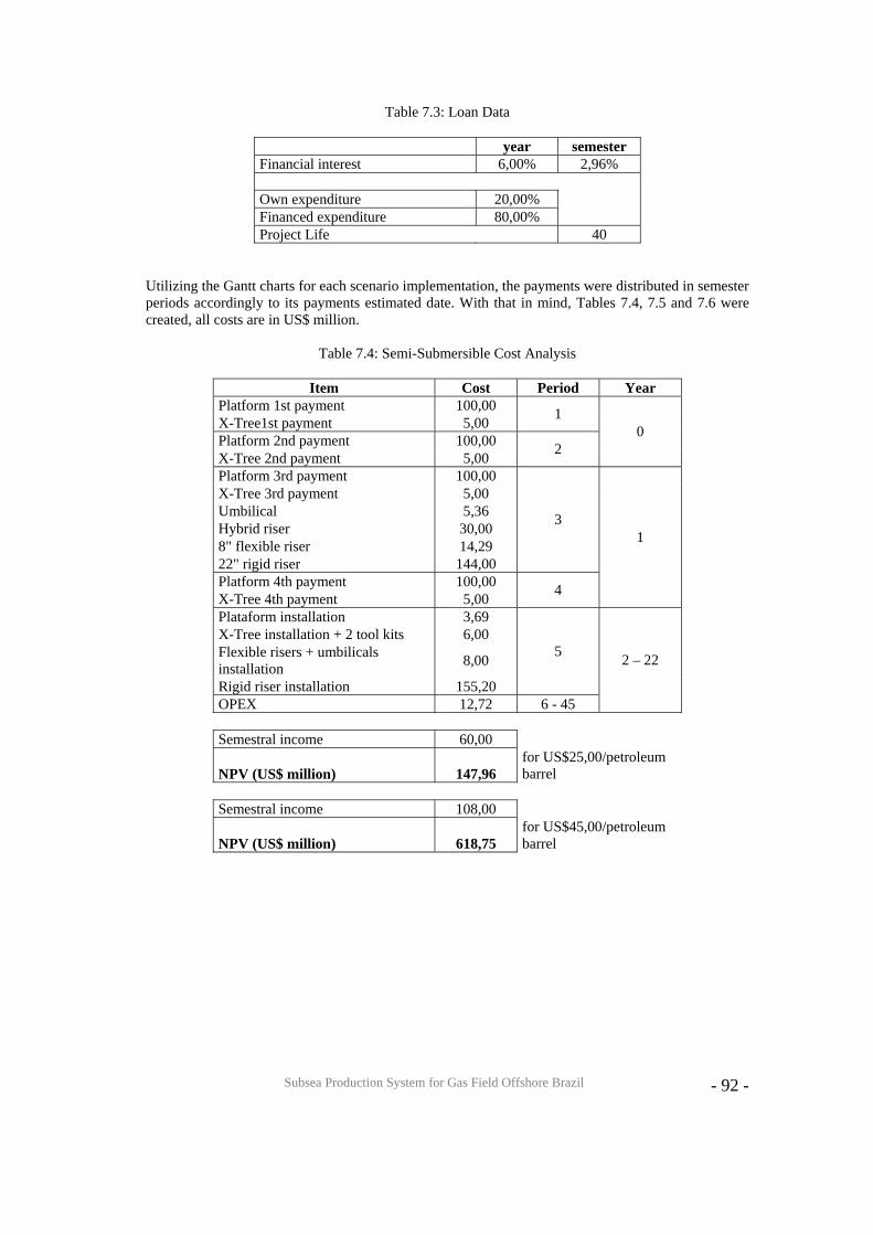
Subsea Production System for Gas Field Offshore Brazil
- 92 -
Table 7.3: Loan Data
year semester Financial interest 6,00% 2,96% Own expenditure 20,00% Financed expenditure 80,00% Project Life 40
Utilizing the Gantt charts for each scenario implementation, the payments were distributed in semester periods accordingly to its payments estimated date. With that in mind, Tables 7.4, 7.5 and 7.6 were created, all costs are in US$ million.
Table 7.4: Semi-Submersible Cost Analysis
Item Cost Period Year
Platform 1st payment 100,00 X-Tree1st payment 5,00 1
Platform 2nd payment 100,00 X-Tree 2nd payment 5,00 2
0
Platform 3rd payment 100,00 X-Tree 3rd payment 5,00 Umbilical 5,36 Hybrid riser 30,00 8" flexible riser 14,29 22" rigid riser 144,00
3
Platform 4th payment 100,00 X-Tree 4th payment 5,00 4
1
Plataform installation 3,69 X-Tree installation + 2 tool kits 6,00 Flexible risers + umbilicals installation 8,00
Rigid riser installation 155,20
5
OPEX 12,72 6 - 45
2 – 22
Semestral income 60,00
NPV (US$ million) 147,96 for US$25,00/petroleum barrel
Semestral income 108,00
NPV (US$ million) 618,75 for US$45,00/petroleum barrel
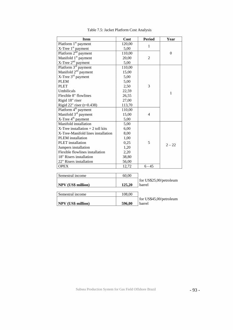
Subsea Production System for Gas Field Offshore Brazil
- 93 -
Table 7.5: Jacket Platform Cost Analysis
Item Cost Period Year Platform 1st payment 120,00 X-Tree 1st payment 5,00 1
Platform 2nd payment 110,00 Manifold 1st payment 20,00 X-Tree 2nd payment 5,00
2 0
Platform 3rd payment 110,00 Manifold 2nd payment 15,00 X-Tree 3rd payment 5,00 PLEM 5,00 PLET 2,50 Umbilicals 22,59 Flexible 8" flowlines 26,55 Rigid 18" riser 27,00 Rigid 22" riser (t=0.438) 113,70
3
Platform 4th payment 110,00 Manifold 3rd payment 15,00 X-Tree 4th payment 5,00
4
1
Manifold installation 5,00 X-Tree installation + 2 toll kits 6,00 X-Tree-Manifold lines installation 8,00 PLEM installation 1,00 PLET installation 0,25 Jumpers installation 1,20 Flexible flowlines installation 2,20 18" Risers installation 38,80 22" Risers installation 56,00
5
OPEX 12,72 6 - 45
2 – 22
Semestral income 60,00
NPV (US$ million) 125,20 for US$25,00/petroleum barrel
Semestral income 108,00
NPV (US$ million) 596,00 for US$45,00/petroleum barrel
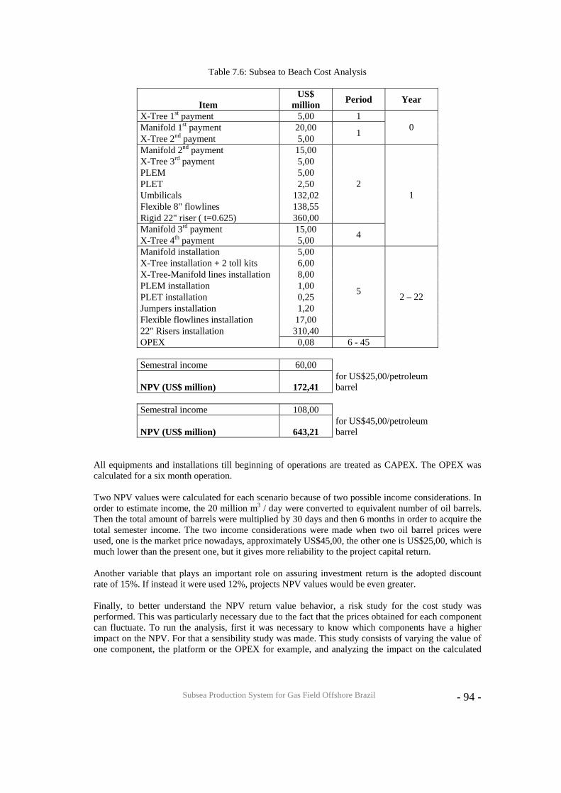
Subsea Production System for Gas Field Offshore Brazil
- 94 -
Table 7.6: Subsea to Beach Cost Analysis
Item US$
million Period Year
X-Tree 1st payment 5,00 1 Manifold 1st payment 20,00 X-Tree 2nd payment 5,00 1 0
Manifold 2nd payment 15,00 X-Tree 3rd payment 5,00 PLEM 5,00 PLET 2,50 Umbilicals 132,02 Flexible 8" flowlines 138,55 Rigid 22" riser ( t=0.625) 360,00
2
Manifold 3rd payment 15,00 X-Tree 4th payment 5,00 4
1
Manifold installation 5,00 X-Tree installation + 2 toll kits 6,00 X-Tree-Manifold lines installation 8,00 PLEM installation 1,00 PLET installation 0,25 Jumpers installation 1,20 Flexible flowlines installation 17,00 22" Risers installation 310,40
5
OPEX 0,08 6 - 45
2 – 22
Semestral income 60,00
NPV (US$ million) 172,41 for US$25,00/petroleum barrel
Semestral income 108,00
NPV (US$ million) 643,21 for US$45,00/petroleum barrel
All equipments and installations till beginning of operations are treated as CAPEX. The OPEX was calculated for a six month operation. Two NPV values were calculated for each scenario because of two possible income considerations. In order to estimate income, the 20 million m3 / day were converted to equivalent number of oil barrels. Then the total amount of barrels were multiplied by 30 days and then 6 months in order to acquire the total semester income. The two income considerations were made when two oil barrel prices were used, one is the market price nowadays, approximately US$45,00, the other one is US$25,00, which is much lower than the present one, but it gives more reliability to the project capital return. Another variable that plays an important role on assuring investment return is the adopted discount rate of 15%. If instead it were used 12%, projects NPV values would be even greater. Finally, to better understand the NPV return value behavior, a risk study for the cost study was performed. This was particularly necessary due to the fact that the prices obtained for each component can fluctuate. To run the analysis, first it was necessary to know which components have a higher impact on the NPV. For that a sensibility study was made. This study consists of varying the value of one component, the platform or the OPEX for example, and analyzing the impact on the calculated
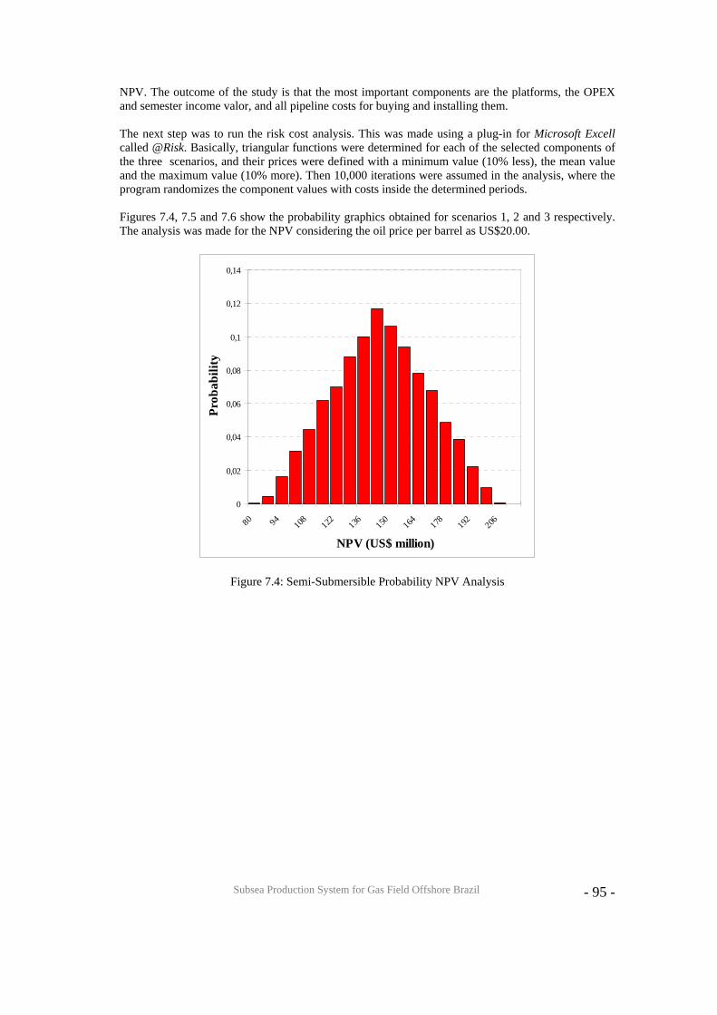
Subsea Production System for Gas Field Offshore Brazil
- 95 -
NPV. The outcome of the study is that the most important components are the platforms, the OPEX and semester income valor, and all pipeline costs for buying and installing them. The next step was to run the risk cost analysis. This was made using a plug-in for Microsoft Excell called @Risk. Basically, triangular functions were determined for each of the selected components of the three scenarios, and their prices were defined with a minimum value (10% less), the mean value and the maximum value (10% more). Then 10,000 iterations were assumed in the analysis, where the program randomizes the component values with costs inside the determined periods. Figures 7.4, 7.5 and 7.6 show the probability graphics obtained for scenarios 1, 2 and 3 respectively. The analysis was made for the NPV considering the oil price per barrel as US$20.00.
0
0,02
0,04
0,06
0,08
0,1
0,12
0,14
80 94108 122 136 150 164 178 192 20
6
NPV (US$ million)
Prob
abili
ty
Figure 7.4: Semi-Submersible Probability NPV Analysis
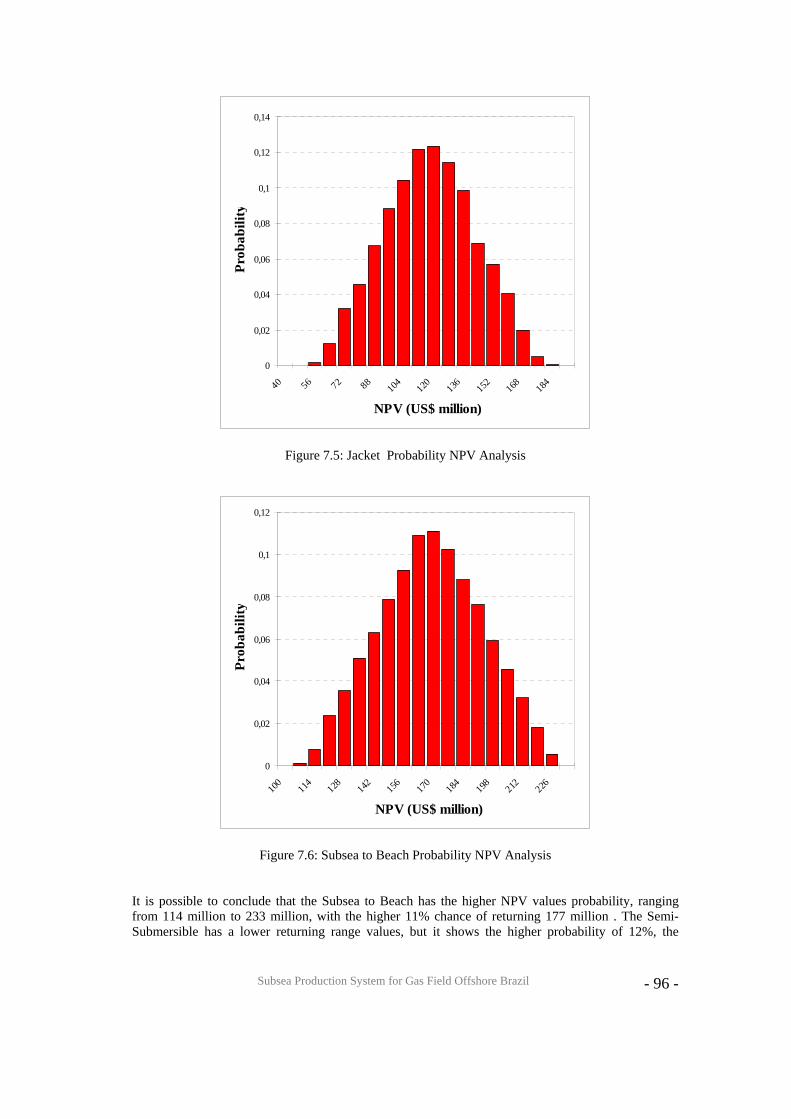
Subsea Production System for Gas Field Offshore Brazil
- 96 -
0
0,02
0,04
0,06
0,08
0,1
0,12
0,14
40 56 72 88104 120 136 152 168 184
NPV (US$ million)
Prob
abili
ty
Figure 7.5: Jacket Probability NPV Analysis
0
0,02
0,04
0,06
0,08
0,1
0,12
100 114 128 142 156 170 184 198 212 226
NPV (US$ million)
Prob
abili
ty
Figure 7.6: Subsea to Beach Probability NPV Analysis It is possible to conclude that the Subsea to Beach has the higher NPV values probability, ranging from 114 million to 233 million, with the higher 11% chance of returning 177 million . The Semi-Submersible has a lower returning range values, but it shows the higher probability of 12%, the
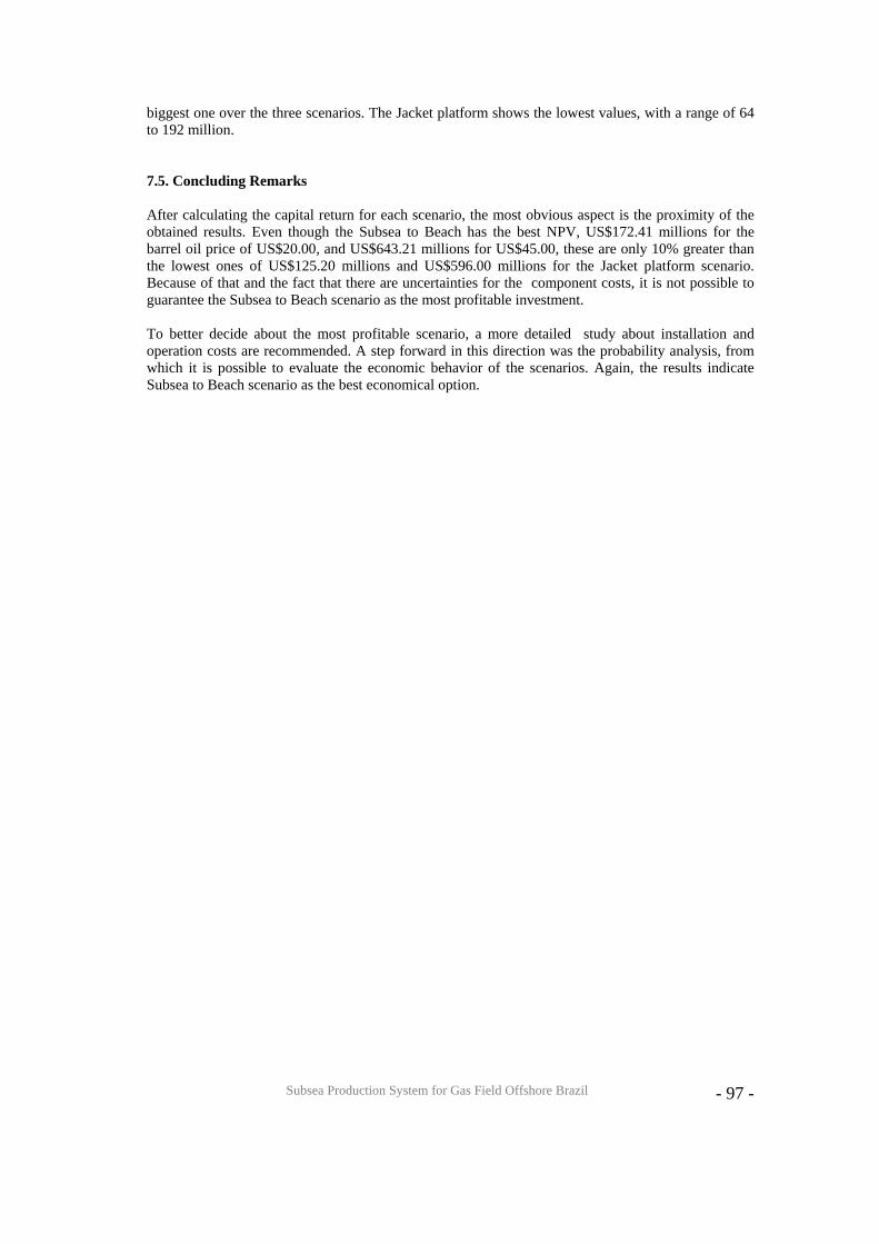
Subsea Production System for Gas Field Offshore Brazil
- 97 -
biggest one over the three scenarios. The Jacket platform shows the lowest values, with a range of 64 to 192 million. 7.5. Concluding Remarks After calculating the capital return for each scenario, the most obvious aspect is the proximity of the obtained results. Even though the Subsea to Beach has the best NPV, US$172.41 millions for the barrel oil price of US$20.00, and US$643.21 millions for US$45.00, these are only 10% greater than the lowest ones of US$125.20 millions and US$596.00 millions for the Jacket platform scenario. Because of that and the fact that there are uncertainties for the component costs, it is not possible to guarantee the Subsea to Beach scenario as the most profitable investment. To better decide about the most profitable scenario, a more detailed study about installation and operation costs are recommended. A step forward in this direction was the probability analysis, from which it is possible to evaluate the economic behavior of the scenarios. Again, the results indicate Subsea to Beach scenario as the best economical option.
Subsea Production System for Gas Field Offshore Brazil
- 98 -
8. CONCLUSIONS Three subsea production systems have been proposed for a gas field offshore Brazil. The considered scenarios considered Semi-submersible platform (SS), Jacket platform (J) and Subsea to Beach (SB). Aspects related to structural integrity, subsea processing, risk assessment and costs have been considered to provide the necessary support for the development of the subsea production systems. In order to analyze the subsea processing different tools, such as OLGA, PIPESIM and analytical solution have been employed for the three scenarios. Based on these results it is realized that the gas mixture can be maintained out of the hydrate envelope by using appropriate pipe insulation. Analyzing Subsea to Beach for the worst case, the longest pipe with flow rate of 10 million m3 per day (by the end of the design life), U value equal to 1.05 W / m2 °C was obtained for the two 22” pipelines. Flow assurance are feasible for all scenarios. The most critical scenario is the SB because it needs either pipeline insulation or MEG continuous injection. Structural and strength analyzes have been performed for the flowlines and risers in order to determine thickness requirements for the rigid steel pipes and to verify the structural response of flexible pipes in relation to the limit values provided by the manufacturer. The critical structural check is related with the dynamic risers in the SS scenario. Extreme loading represented by wave and current loads were considered in the analyzes. The results indicated both tensile forces and curvature radius within the safety margins. Installation procedures have been discussed in relation to flowlines/risers, X-trees and manifolds. Due to the pipeline diameters (18” and 22”) J-lay method is recommended. For the flexible pipes (8”) the conventional reel installation is indicated. X-trees and manifolds are to be installed diverless due to the water depth of 500 m. In the case of the X-trees the guidelineless procedure associated with vertical control module is recommended to allow independency between flowline and X-Tree installations, reducing costs with additional vessel mobilization. Risk assessment has been conducted for production loss. Fault trees constructed for each scenario have been analyzed in terms of qualitative risk approach. The conceptual probability of failure for the total production loss indicates that scenario 1 presents the best result. The satellite wells contribute to decrease the probability of a shut down. The possibility of a shut down depends on export pipe system failure. For scenarios 2 and 3, there are additional possibilities of failure associated with subsea multiplexed control and manifold. In relation to the total production loss it was concluded that the most reliable subsea arrangement system is that represented by scenario 1, followed by scenarios 3 and 2. The partial production loss considers only one well interruption. Analyzing the subsea arrangements and respective fault trees it can be observed that scenarios 2 and 3 are more reliable than scenario 1. As already mentioned the advantage of on-bottom import system using manifolds and electro-hydraulic multiplex control reflects on smaller failure probability if compared with the import and export dynamic risers in scenario 1. In general, it can be concluded that scenarios 2 and 3 are more reliable than scenario 1 for partial production loss. In this case it is difficult to distinguish scenarios 2 and 3. Although scenario 3 has two redundant export pipelines, the transport of water/gas mixture increases the probability of hydrate formation if compared with scenario 2, although in this scenario there is no pipeline redundancy. Considering that the total production loss is associated with a failure probability substantially smaller than for the partial production loss, the indication of the most reliable scenario should take into consideration small production losses during the project life cycle. The satellite wells associated with dynamic risers put the scenario 1 as the less attractive alternative. Although equivalent in terms of partial production loss, scenario 3 is more reliable than scenario 2 for total production loss. Therefore,
Subsea Production System for Gas Field Offshore Brazil
- 99 -
based on the qualitative risk assessment for production loss, the scenario 3 can be indicated as the best option for the offshore gas field considered in this project. However, the possibility of gas/water subsea separation and subsea gas compression, before export to onshore terminal, could mean an outstanding advantage for Subsea to Beach scenario in relation to both Semi-submersible and Jacket scenarios. Cost analysis indicates close capital returns for the three scenarios. Subsea to Beach has the best NPV, US$172.41 millions for the oil barrel oil of US$20.00, and US$643.21 millions for US$45.00. These are only 10% greater than the lowest ones for the Jacket scenario. As general conclusion the Subsea to Beach scenario is the best option according to the main results from the project. However, additional technological developments associated with subsea gas/water separation and subsea gas compression are strongly recommended in order to have this option commercially available in the near future. Aspects related to subsea equipment reliability and remote control are also of paramount importance for the unmanned Subsea to Beach concept.
Subsea Production System for Gas Field Offshore Brazil
- 100 -
9. REFERENCES [1] Su J., Regis, C. R. and Botto A. Thermal analysis of combined active heating and passive insulation of deepwater pipelines. OMAE 02/ Pipe-28491,2002. [2] PIPESIM User Guide , Baker Jardine Petroleum & Software,2000. [3] Borrehaug, A., Loken, K-P, Raghavendra, K. and Waalmann, J.G. – Deepwater subsea to beach gas developments- Flow Assurance Challenges and Solutions, DOT, New Orleans, 2004 [4] Wilson, A., Holm, H. Ormen Lange – Flow assurance challenges, OTC 16555, 2004. [5] Det Norske Veritas. Submarine pipeline systems. Offshore Standard, Norway, 2000. [6] American Petroleum Institute (API 5L) – Specification for Line Pipe – 2000. [7] ANFLEX4914/ User’s Manual – Version 5.7, CENPES/PDEP/MC, December, 2001. [8] Petrobras`s Technical Specification ET-3549.00-6500-291-PPC-001- Rev A, 2001. [9] Petrobras`s Technical Specification ET-3010.00-1500-960-PPC-003- Rev 0, 2000. [10] American Petroleum Institute – Design of Risers for Floating Production Systems (FPSs) – Recommended Practice 2RD – First Edition, 1998. [11] Castello, X. – Effects of the Installation Process on the Structural Strength of Sandwich Pipes, M.Sc. Thesis, COPPE/UFRJ, 2005 (In Portuguese). [12] Labanca, E.L. – Methodology to Select Subsea Layout Based on Operational Efficiency, M.Sc. Thesis, COPPE/UFRJ, 2005 (In Portuguese). [13] Albernaz, R.S. – Data Bank Proposition for Wet Christmas Tree Reliability Study, M.Sc. Thesis, COPPE/UFRJ, 2005 (In Portuguese). [14] Garcia, J.E.L. and Figueiredo, M.W. – Wet Christmas Tree, Petrobras Notes, 1999. [15] Fantoft, R. and Hendriks, T. – Deepwater subsea separation – Technical challenges and solutions, DOT, New Orleans, 2004. [16] Rausand, M. – Risk and Reliability in Subsea Engineering, Technical Notes, NTNU, August 1999. [17] Kuo, C. – Managing Ship Safety, LLP ed., London, 1998. [18] American Bureau of Shipping – Guide for Risk Evaluation for the Classification of Marine-Related Facilities, June 2003. [19] Gustavsson, F., Eriksen, R. and Anthonsen, H. – Developing an offshore inspection, maintenance and repair strategy for Ormen Lange, DOT, New Orleans, 2004.
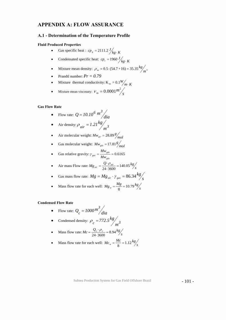
Subsea Production System for Gas Field Offshore Brazil
- 101 -
APPENDIX A: FLOW ASSURANCE A.1 - Determination of the Temperature Profile
Fluid Produced Properties
• Gas specific heat : KkgJcpg ⋅= 2.2111
• Condensated specific heat: KkgJcpc ⋅=1960
• Mixture mean density: 335.3516)+(54.70.5m
kgm =⋅=ρ
• Prandtl number: 0.79=Pr • Mixture thermal conductivity: Km
W⋅0.1=K m
• Mixture mean viscosuty: sm2
m 0.0001=ν
Gas Flow Rate
• Flow rate: diam10.10Q
36=
• Air density: 3air mkg21.1=ρ
• Air molecular weight: molgMwair 89.28=
• Gas molecular weight: molgMwgás 81.17=
• Gas relative gravity: 6165.0==gás
gásgas Mw
Mwγ
• Air mass Flow rate: skgQ
Mg airair 05.140
360024=
⋅⋅
=ρ
• Gas mass flow rate: skgMgMg gasair 34.86=⋅= γ
• Mass flow rate for each well: skgMg
Mg w 79.108
==
Condensed Flow Rate
• Flow rate: diam1000Q
3c =
• Condensed density: 3c mkg5.772=ρ
• Mass flow rate: skgQ
Mc cc 94.8360024
=⋅⋅
=ρ
• Mass flow rate for each well: skgMcMcw 12.1
8==
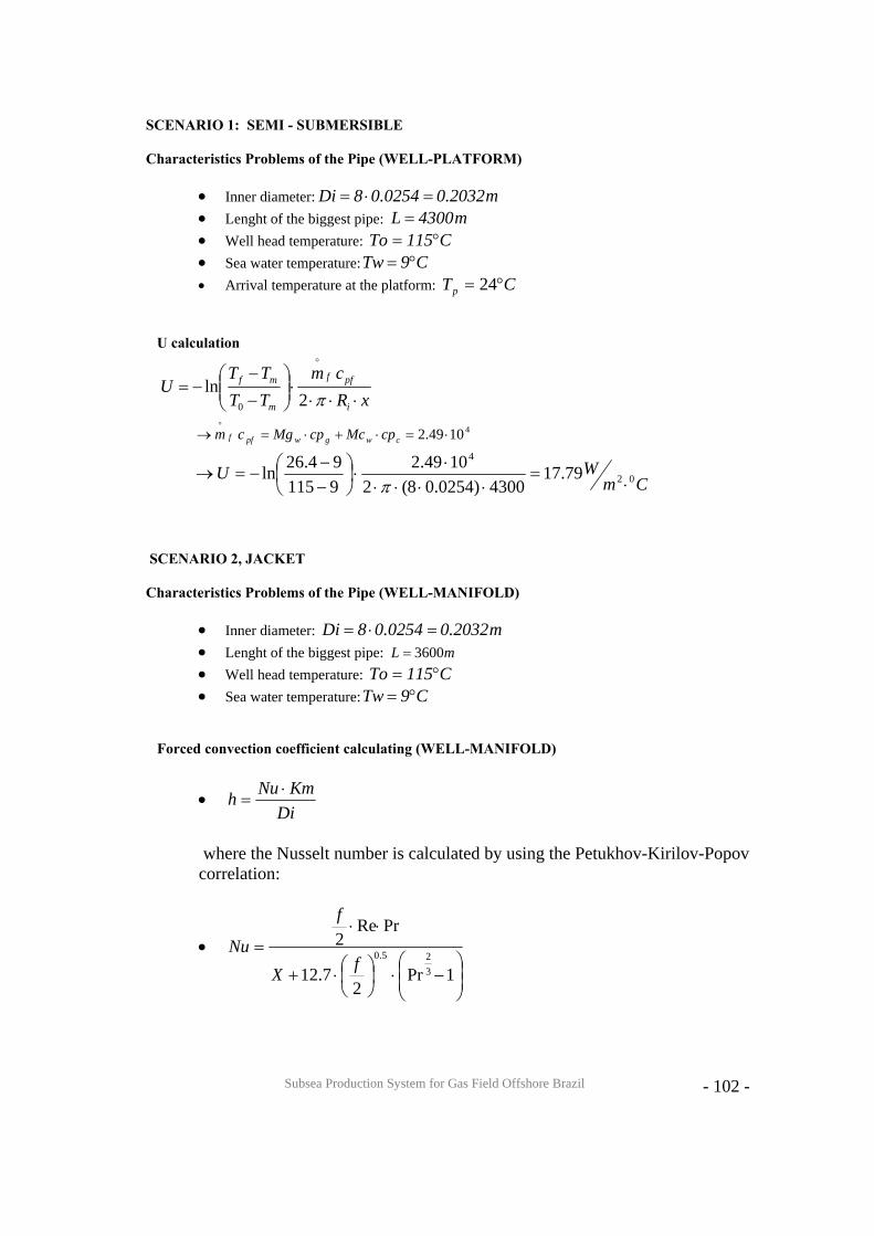
Subsea Production System for Gas Field Offshore Brazil
- 102 -
SCENARIO 1: SEMI - SUBMERSIBLE Characteristics Problems of the Pipe (WELL-PLATFORM)
• Inner diameter: m2032.00254.08Di =⋅= • Lenght of the biggest pipe: m4300L = • Well head temperature: C115To °= • Sea water temperature: C9Tw °= • Arrival temperature at the platform: CTp °= 24
U calculation
xRcm
TTTT
Ui
pff
m
mf
⋅⋅⋅⋅⎟⎟⎠
⎞⎜⎜⎝
⎛−
−−=
π2ln
0
o
41049.2 ⋅=⋅+⋅=→ cwgwpff cpMccpMgcmo
CmWU 02
4
79.174300)0254.08(2
1049.2911594.26ln
⋅=
⋅⋅⋅⋅⋅
⋅⎟⎠⎞
⎜⎝⎛
−−
−=→π
SCENARIO 2, JACKET Characteristics Problems of the Pipe (WELL-MANIFOLD)
• Inner diameter: m2032.00254.08Di =⋅= • Lenght of the biggest pipe: mL 3600= • Well head temperature: C115To °= • Sea water temperature: C9Tw °=
Forced convection coefficient calculating (WELL-MANIFOLD)
• Di
KmNuh ⋅=
where the Nusselt number is calculated by using the Petukhov-Kirilov-Popov correlation:
•
⎟⎟⎠
⎞⎜⎜⎝
⎛−⋅⎟
⎠⎞
⎜⎝⎛⋅+
⋅⋅=
1Pr2
7.12
PrRe2
325.0fX
f
Nu
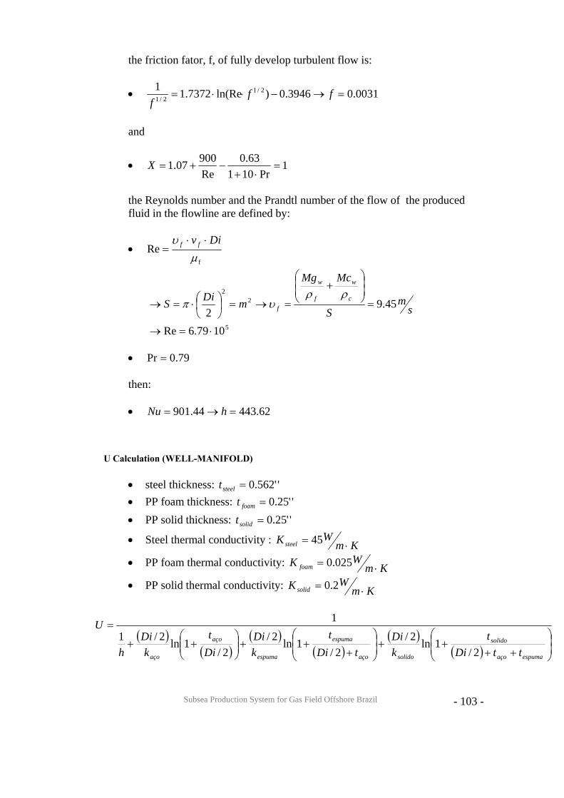
Subsea Production System for Gas Field Offshore Brazil
- 103 -
the friction fator, f, of fully develop turbulent flow is:
• 0031.03946.0)ln(Re7372.11 2/12/1 =→−⋅⋅= ff
f
and
• 1Pr101
63.0Re90007.1 =
⋅+−+=X
the Reynolds number and the Prandtl number of the flow of the produced fluid in the flowline are defined by:
• f
Reµ
υ Div ff ⋅⋅=
5
22
1079.6Re
45.92⋅=→
=⎟⎟⎠
⎞⎜⎜⎝
⎛+
=→=⎟⎠⎞
⎜⎝⎛⋅=→ s
mS
McMg
mDiS c
w
f
w
f
ρρυπ
• 79.0Pr = then: • 62.44344.901 =→= hNu
U Calculation (WELL-MANIFOLD)
• steel thickness: ''562.0=steelt • PP foam thickness: ''25.0=foamt • PP solid thickness: ''25.0=solidt
• Steel thermal conductivity : KmWKsteel ⋅= 45
• PP foam thermal conductivity: KmWK foam ⋅= 025.0
• PP solid thermal conductivity: KmWKsolid ⋅= 2.0
( )( )
( )( )
( )( ) ⎟
⎟⎠
⎞⎜⎜⎝
⎛
++++⎟
⎟⎠
⎞⎜⎜⎝
⎛
+++⎟⎟
⎠
⎞⎜⎜⎝
⎛++
=
espumaaço
solido
solidoaço
espuma
espuma
aço
aço ttDit
kDi
tDit
kDi
Dit
kDi
h
U
2/1ln2/
2/1ln2/
2/1ln2/1
1
Subsea Production System for Gas Field Offshore Brazil
- 104 -
KmWU
⋅= 284.3
Determination of the Temperature Profile (WELL-MANIFOLD)
• ( )⎟⎟⎟
⎠
⎞
⎜⎜⎜
⎝
⎛⋅⋅⋅
−⋅−+=
pff
imm
cm
xUDTTTT
o
πexp0
( ) CUT 044.832.24975
3600)0254.08(exp91159)3600( =⎟⎠⎞
⎜⎝⎛ ⋅⋅⋅⋅−⋅−+=→π
Characteristics problems of the pipe (PLEM-JACKET)
• Inner diameter: mDi 4572.00254.018 =⋅= • Lenght of the biggest pipe: mL 20000= • Exit PLEM temperature: CTTo °=−= 53.1031)3600( • Sea water temperature: CTm °= 9
Convection Coefficient Calculating (PLEM - JACKET)
• 79.0Pr =
sm
S
McMg
mDiS c
w
f
w
f 93.142
22
=⎟⎟⎠
⎞⎜⎜⎝
⎛+
=→=⎟⎠⎞
⎜⎝⎛⋅=→
ρρυπ
• 61041.2Re ⋅=
• 999.0Pr101
63.0Re90007.1 =
⋅+−+=X
• 99.03946.0)ln(Re7372.11 2/12/1 =→−⋅⋅= ff
f
• 31811Pr
27.12
PrRe2
325.0 =
⎟⎟⎠
⎞⎜⎜⎝
⎛−⋅⎟
⎠⎞
⎜⎝⎛⋅+
⋅⋅=
fX
f
Nu
• 74.695=h
Subsea Production System for Gas Field Offshore Brazil
- 105 -
U calculation (PLEM- JACKET)
( )( )
( )( )
( )( ) ⎟
⎟⎠
⎞⎜⎜⎝
⎛
++++⎟
⎟⎠
⎞⎜⎜⎝
⎛
+++⎟⎟
⎠
⎞⎜⎜⎝
⎛++
=
espumaaço
solido
solidoaço
espuma
espuma
aço
aço ttDit
kDi
tDit
kDi
Dit
kDi
h
U
2/1ln2/
2/1ln2/
2/1ln2/1
1
KmWU
⋅= 278.3
Determination of the Temperature Profile (PLEM-JACKET)
• ( )⎟⎟⎟
⎠
⎞
⎜⎜⎜
⎝
⎛⋅⋅⋅
−⋅−+=
pff
imm
cm
xUDTTTT
o
πexp0
( ) CUT 071.3399900.6
20000)0254.018(exp953.1039)20000( =⎟⎠⎞
⎜⎝⎛ ⋅⋅⋅⋅−⋅−+=→π
Scenario 3: SUBSEA TO BEACH Characteristics problems of the pipe (WELL-MANIFOLD)
• Inner diameter: m2032.00254.08Di =⋅= • Lenght of the biggest pipe: mL 3600= • Well head temperature: C115To °= • Sea water temperature: C9Tw °=
Forced Convection Coefficient Calculating (WELL - MANIFOLD)
• 79.0Pr =
sm
S
McMg
mDiS c
w
f
w
f 45.92
22
=⎟⎟⎠
⎞⎜⎜⎝
⎛+
=→=⎟⎠⎞
⎜⎝⎛⋅=→
ρρυπ
• 51079.6Re ⋅=
• =⋅+
−+=Pr101
63.0Re90007.1X
• 0031.03946.0)ln(Re7372.11 2/12/1 =→−⋅⋅= ff
f
Subsea Production System for Gas Field Offshore Brazil
- 106 -
• 44.9011Pr
27.12
PrRe2
325.0 =
⎟⎟⎠
⎞⎜⎜⎝
⎛−⋅⎟
⎠⎞
⎜⎝⎛⋅+
⋅⋅=
fX
f
Nu
• 62.443=h
U Calculation (WELL - MANIFOLD)
( )( )
( )( )
( )( ) ⎟
⎟⎠
⎞⎜⎜⎝
⎛
++++⎟
⎟⎠
⎞⎜⎜⎝
⎛
+++⎟⎟
⎠
⎞⎜⎜⎝
⎛++
=
espumaaço
solido
solidoaço
espuma
espuma
aço
aço ttDit
kDi
tDit
kDi
Dit
kDi
h
U
2/1ln2/
2/1ln2/
2/1ln2/1
1
KmWU
⋅= 2299.1
Determination of the Temperature Profile (WELL-MANIFOLD):
• ( )⎟⎟⎟
⎠
⎞
⎜⎜⎜
⎝
⎛⋅⋅⋅
−⋅−+=
pff
imm
cm
xUDTTTT
o
πexp0
( ) Ccm
UTpff
053.1043600)0254.08(exp91159)3600( =⎟⎟⎟
⎠
⎞
⎜⎜⎜
⎝
⎛⋅⋅⋅⋅
−⋅−+=→o
π
Characteristics Problems of the Pipe (PLEM-TERMINAL):
• Inner diameter: mDi 5588.00254.022 =⋅= • Lenght of the biggest pipe: mL 160000= • Exit PLEM temperature: CTTo °=−= 53.1031)3600( • Sea water temperature: CTm °= 9
Forced Convection Coefficient Calculating (PLEM - TERMINAL)
• 79.0Pr =
sm
S
McMg
mDiS c
w
f
w
f 102
22
=⎟⎟⎠
⎞⎜⎜⎝
⎛+
=→=⎟⎠⎞
⎜⎝⎛⋅=→
ρρυπ
• 61097.1Re ⋅=
Subsea Production System for Gas Field Offshore Brazil
- 107 -
• 999.0Pr101
63.0Re90007.1 =
⋅+−+=X
• 0026.03946.0)ln(Re7372.11 2/12/1 =→−⋅⋅= ff
f
• 7.7471Pr
27.12
PrRe2
325.0 =
⎟⎟⎠
⎞⎜⎜⎝
⎛−⋅⎟
⎠⎞
⎜⎝⎛⋅+
⋅⋅=
fX
f
Nu
• .133=h
U Calculation (PLEM - TERMINAL)
( )( )
( )( )
( )( ) ⎟
⎟⎠
⎞⎜⎜⎝
⎛
++++⎟
⎟⎠
⎞⎜⎜⎝
⎛
+++⎟⎟
⎠
⎞⎜⎜⎝
⎛++
=
espumaaço
solido
solidoaço
espuma
espuma
aço
aço ttDit
kDi
tDit
kDi
Dit
kDi
h
U
2/1ln2/
2/1ln2/
2/1ln2/1
1
KmWU
⋅= 2047.1
Determination of the Temperature Profile (PLEM - TERMINAL)
• ( )⎟⎟⎟
⎠
⎞
⎜⎜⎜
⎝
⎛⋅⋅⋅
−⋅−+=
pff
imm
cm
xUDTTTT
o
πexp0
( ) CUT 09.136.99900
20000)0254.022(exp953.1039)160000( =⎟⎠⎞
⎜⎝⎛ ⋅⋅⋅⋅−⋅−+=→π
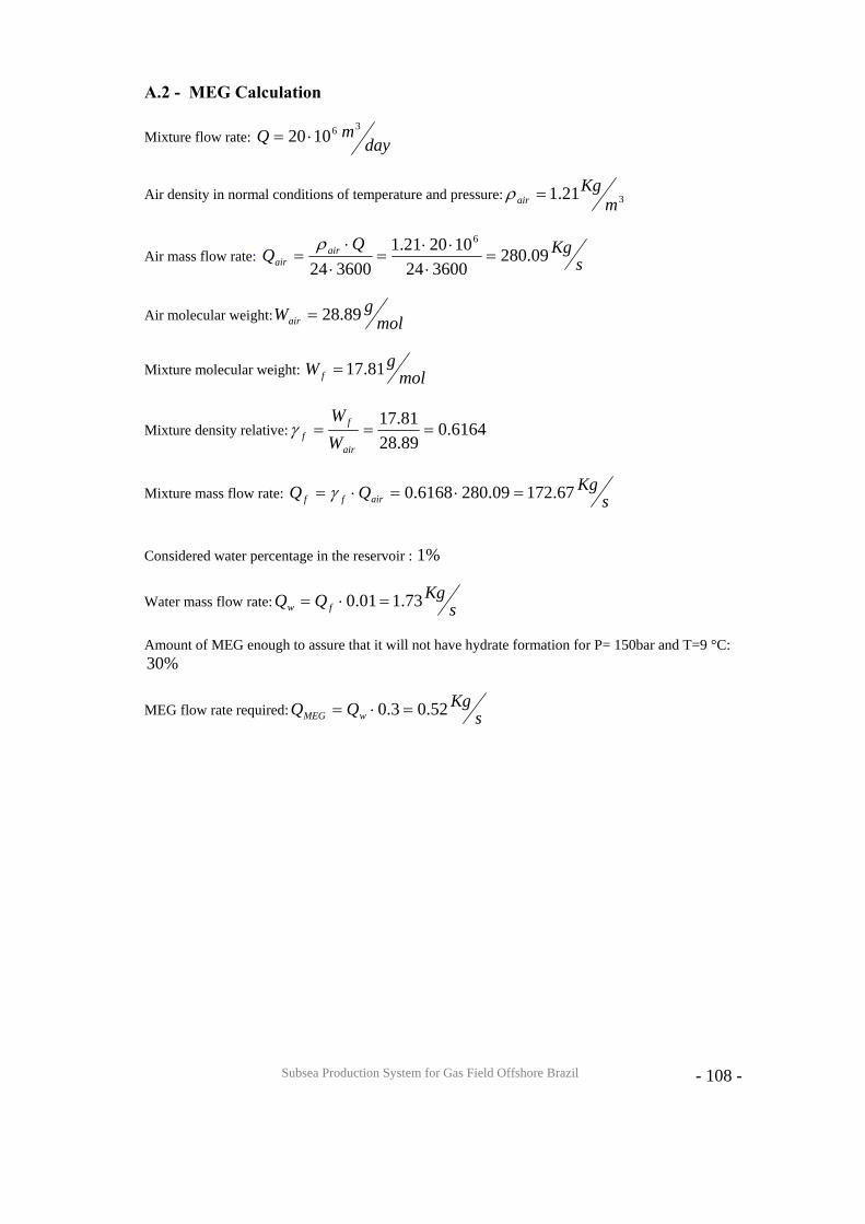
Subsea Production System for Gas Field Offshore Brazil
- 108 -
A.2 - MEG Calculation
Mixture flow rate: daymQ
361020 ⋅=
Air density in normal conditions of temperature and pressure: 321.1 mKg
air =ρ
Air mass flow rate: sKgQ
Q airair 09.280
360024102021.1
360024
6
=⋅
⋅⋅=
⋅⋅
=ρ
Air molecular weight: molgWair 89.28=
Mixture molecular weight: molgW f 81.17=
Mixture density relative: 6164.089.2881.17
===air
ff W
Wγ
Mixture mass flow rate: sKgQQ airff 67.17209.2806168.0 =⋅=⋅= γ
Considered water percentage in the reservoir : %1
Water mass flow rate: sKgQQ fw 73.101.0 =⋅=
Amount of MEG enough to assure that it will not have hydrate formation for P= 150bar and T=9 °C:
%30
MEG flow rate required: sKgQQ wMEG 52.03.0 =⋅=
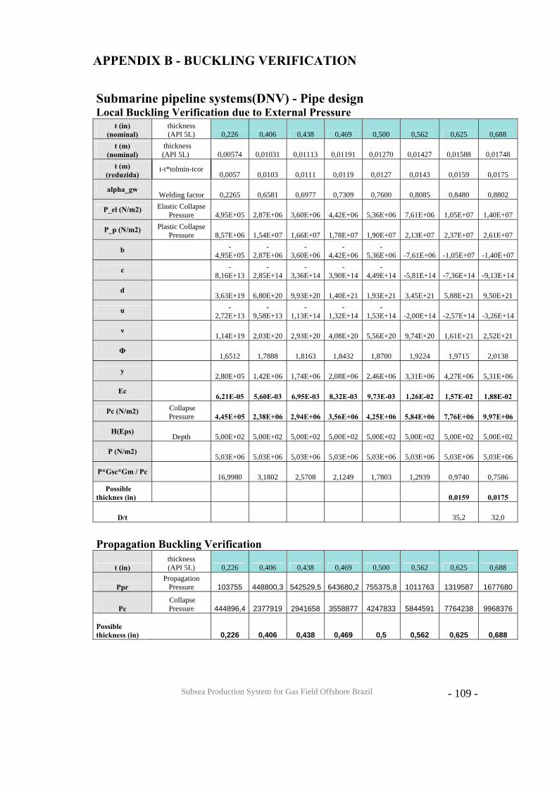
Subsea Production System for Gas Field Offshore Brazil
- 109 -
APPENDIX B - BUCKLING VERIFICATION
Submarine pipeline systems(DNV) - Pipe design Local Buckling Verification due to External Pressure
t (in) (nominal)
thickness (API 5L) 0,226 0,406 0,438 0,469 0,500 0,562 0,625 0,688
t (m) (nominal)
thickness (API 5L) 0,00574 0,01031 0,01113 0,01191 0,01270 0,01427 0,01588 0,01748
t (m) (reduzida)
t-t*tolmin-tcor 0,0057 0,0103 0,0111 0,0119 0,0127 0,0143 0,0159 0,0175
alpha_gw Welding factor 0,2265 0,6581 0,6977 0,7309 0,7600 0,8085 0,8480 0,8802
P_el (N/m2) Elastic Collapse Pressure 4,95E+05 2,87E+06 3,60E+06 4,42E+06 5,36E+06 7,61E+06 1,05E+07 1,40E+07
P_p (N/m2) Plastic Collapse Pressure 8,57E+06 1,54E+07 1,66E+07 1,78E+07 1,90E+07 2,13E+07 2,37E+07 2,61E+07
b
-4,95E+05
-2,87E+06
-3,60E+06
-4,42E+06
-5,36E+06 -7,61E+06 -1,05E+07 -1,40E+07
c
-8,16E+13
-2,85E+14
-3,36E+14
-3,90E+14
-4,49E+14 -5,81E+14 -7,36E+14 -9,13E+14
d 3,63E+19 6,80E+20 9,93E+20 1,40E+21 1,93E+21 3,45E+21 5,88E+21 9,50E+21
u
-2,72E+13
-9,58E+13
-1,13E+14
-1,32E+14
-1,53E+14 -2,00E+14 -2,57E+14 -3,26E+14
ν 1,14E+19 2,03E+20 2,93E+20 4,08E+20 5,56E+20 9,74E+20 1,61E+21 2,52E+21
Ф 1,6512 1,7888 1,8163 1,8432 1,8700 1,9224 1,9715 2,0138
y 2,80E+05 1,42E+06 1,74E+06 2,08E+06 2,46E+06 3,31E+06 4,27E+06 5,31E+06
Ec 6,21E-05 5,60E-03 6,95E-03 8,32E-03 9,73E-03 1,26E-02 1,57E-02 1,88E-02
Pc (N/m2) Collapse Pressure 4,45E+05 2,38E+06 2,94E+06 3,56E+06 4,25E+06 5,84E+06 7,76E+06 9,97E+06
H(Eps) Depth 5,00E+02 5,00E+02 5,00E+02 5,00E+02 5,00E+02 5,00E+02 5,00E+02 5,00E+02
P (N/m2) 5,03E+06 5,03E+06 5,03E+06 5,03E+06 5,03E+06 5,03E+06 5,03E+06 5,03E+06
P*Gsc*Gm / Pc 16,9980 3,1802 2,5708 2,1249 1,7803 1,2939 0,9740 0,7586
Possible thicknes (in) 0,0159 0,0175
D/t 35,2 32,0
Propagation Buckling Verification
t (in) thickness (API 5L) 0,226 0,406 0,438 0,469 0,500 0,562 0,625 0,688
Ppr Propagation
Pressure 103755 448800,3 542529,5 643680,2 755375,8 1011763 1319587 1677680
Pc Collapse Pressure 444896,4 2377919 2941658 3558877 4247833 5844591 7764238 9968376
Possible thickness (in) 0,226 0,406 0,438 0,469 0,5 0,562 0,625 0,688
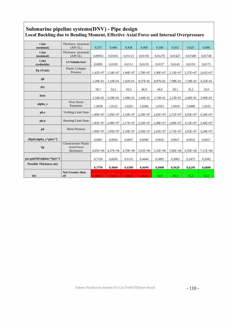
Subsea Production System for Gas Field Offshore Brazil
- 110 -
Submarine pipeline systems(DNV) - Pipe design Local Buckling due to Bending Moment, Effective Axial Force and Internal Overpressure
t (in) (nominal)
Thickness (nominal) (API 5L) 0,375 0,406 0,438 0,469 0,500 0,562 0,625 0,688
t (in) (nominal)
Thickness (nominal) (API 5L) 0,00953 0,01031 0,01113 0,01191 0,01270 0,01427 0,01588 0,01748
t (m) (reduzida)
t-t*tolmin-tcor 0,0095 0,0103 0,0111 0,0119 0,0127 0,0143 0,0159 0,0175
Pp (N/m2) Plastic Collapse Pressure 1,42E+07 1,54E+07 1,66E+07 1,78E+07 1,90E+07 2,13E+07 2,37E+07 2,61E+07
qh 1,20E-01 1,10E-01 1,02E-01 9,57E-02 8,97E-02 7,98E-02 7,18E-02 6,52E-02
D/t 58,7 54,2 50,2 46,9 44,0 39,1 35,2 32,0
beta 1,54E-02 6,59E-02 1,09E-01 1,44E-01 1,74E-01 2,22E-01 2,60E-01 2,90E-01
alpha_c Flow Stress Parameter 1,0028 1,0122 1,0201 1,0266 1,0321 1,0410 1,0480 1,0535
pb,s Yielding Limit State 1,80E+07 1,95E+07 2,10E+07 2,26E+07 2,41E+07 2,71E+07 3,03E+07 3,34E+07
pb,u Bursting Limit State 1,85E+07 2,00E+07 2,17E+07 2,32E+07 2,48E+07 2,80E+07 3,12E+07 3,44E+07
pb Burst Pressure 1,80E+07 1,95E+07 2,10E+07 2,26E+07 2,41E+07 2,71E+07 3,03E+07 3,34E+07
(Dpd/(alpha_c*pb))^2 0,0067 0,0056 0,0047 0,0040 0,0035 0,0027 0,0022 0,0017
Sp Characteristic Plastic
Axial Force Resistance 4,05E+06 4,37E+06 4,70E+06 5,02E+06 5,33E+06 5,96E+06 6,59E+06 7,21E+06
gsc.gm(Sd/(alphac*Sp))^2 0,7159 0,6030 0,5131 0,4444 0,3891 0,3063 0,2472 0,2043
Possible Thickness (m) 0,3750 0,4060 0,4380 0,4690 0,5000 0,5620 0,6250 0,6880
D/t Not Greater than 45 58,7 54,2 50,2 46,9 44,0 39,1 35,2 32,0
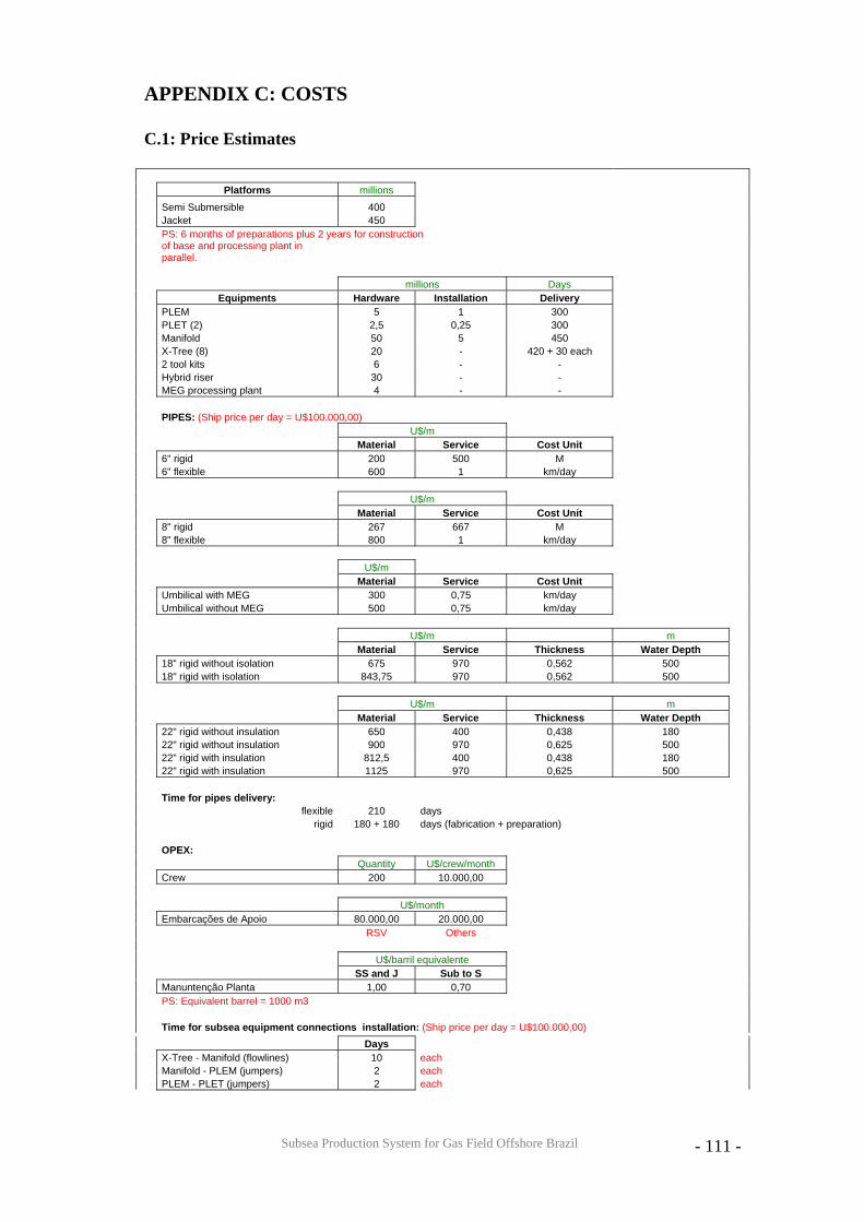
Subsea Production System for Gas Field Offshore Brazil
- 111 -
APPENDIX C: COSTS C.1: Price Estimates
Platforms millions
Semi Submersible 400 Jacket 450 PS: 6 months of preparations plus 2 years for construction
of base and processing plant in parallel.
millions Days Equipments Hardware Installation Delivery PLEM 5 1 300 PLET (2) 2,5 0,25 300 Manifold 50 5 450 X-Tree (8) 20 - 420 + 30 each 2 tool kits 6 - - Hybrid riser 30 - - MEG processing plant 4 - - PIPES: (Ship price per day = U$100.000,00) U$/m Material Service Cost Unit 6" rigid 200 500 M 6" flexible 600 1 km/day U$/m Material Service Cost Unit 8" rigid 267 667 M 8" flexible 800 1 km/day U$/m Material Service Cost Unit Umbilical with MEG 300 0,75 km/day Umbilical without MEG 500 0,75 km/day U$/m m Material Service Thickness Water Depth 18" rigid without isolation 675 970 0,562 500 18" rigid with isolation 843,75 970 0,562 500 U$/m m Material Service Thickness Water Depth 22" rigid without insulation 650 400 0,438 180 22" rigid without insulation 900 970 0,625 500 22" rigid with insulation 812,5 400 0,438 180 22" rigid with insulation 1125 970 0,625 500 Time for pipes delivery: flexible 210 days rigid 180 + 180 days (fabrication + preparation) OPEX: Quantity U$/crew/month Crew 200 10.000,00 U$/month Embarcações de Apoio 80.000,00 20.000,00 RSV Others U$/barril equivalente SS and J Sub to S Manuntenção Planta 1,00 0,70 PS: Equivalent barrel = 1000 m3 Time for subsea equipment connections installation: (Ship price per day = U$100.000,00) Days X-Tree - Manifold (flowlines) 10 each Manifold - PLEM (jumpers) 2 each PLEM - PLET (jumpers) 2 each
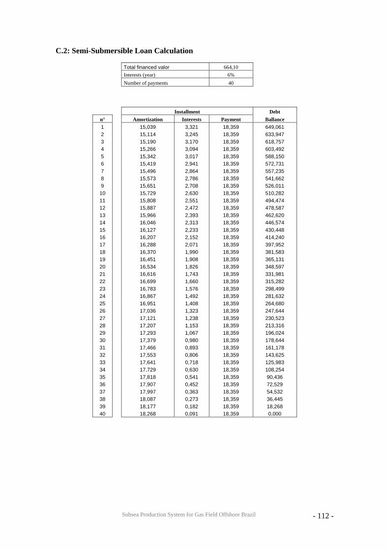
Subsea Production System for Gas Field Offshore Brazil
- 112 -
C.2: Semi-Submersible Loan Calculation
Total financed valor 664,10 Interests (year) 6% Number of payments 40
Installment Debt n° Amortization Interests Payment Ballance 1 15,039 3,321 18,359 649,061 2 15,114 3,245 18,359 633,947 3 15,190 3,170 18,359 618,757 4 15,266 3,094 18,359 603,492 5 15,342 3,017 18,359 588,150 6 15,419 2,941 18,359 572,731 7 15,496 2,864 18,359 557,235 8 15,573 2,786 18,359 541,662 9 15,651 2,708 18,359 526,011
10 15,729 2,630 18,359 510,282 11 15,808 2,551 18,359 494,474 12 15,887 2,472 18,359 478,587 13 15,966 2,393 18,359 462,620 14 16,046 2,313 18,359 446,574 15 16,127 2,233 18,359 430,448 16 16,207 2,152 18,359 414,240 17 16,288 2,071 18,359 397,952 18 16,370 1,990 18,359 381,583 19 16,451 1,908 18,359 365,131 20 16,534 1,826 18,359 348,597 21 16,616 1,743 18,359 331,981 22 16,699 1,660 18,359 315,282 23 16,783 1,576 18,359 298,499 24 16,867 1,492 18,359 281,632 25 16,951 1,408 18,359 264,680 26 17,036 1,323 18,359 247,644 27 17,121 1,238 18,359 230,523 28 17,207 1,153 18,359 213,316 29 17,293 1,067 18,359 196,024 30 17,379 0,980 18,359 178,644 31 17,466 0,893 18,359 161,178 32 17,553 0,806 18,359 143,625 33 17,641 0,718 18,359 125,983 34 17,729 0,630 18,359 108,254 35 17,818 0,541 18,359 90,436 36 17,907 0,452 18,359 72,529 37 17,997 0,363 18,359 54,532 38 18,087 0,273 18,359 36,445 39 18,177 0,182 18,359 18,268 40 18,268 0,091 18,359 0,000
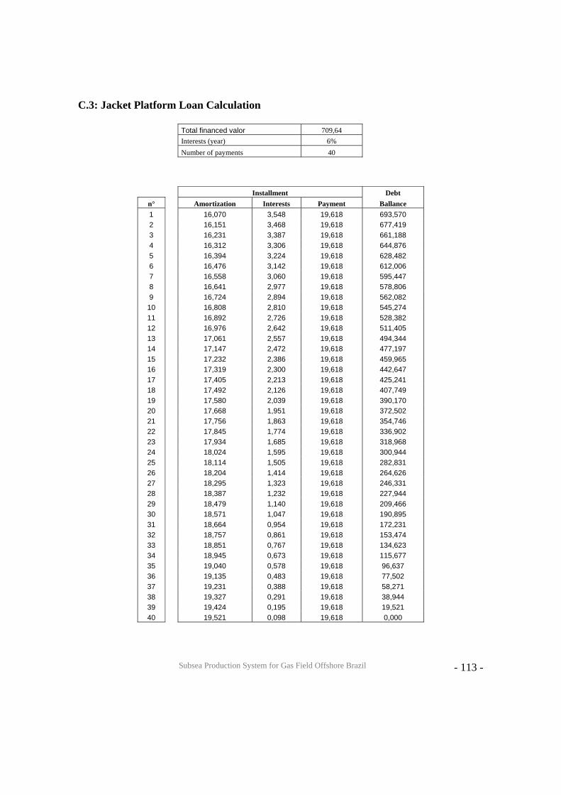
Subsea Production System for Gas Field Offshore Brazil
- 113 -
C.3: Jacket Platform Loan Calculation
Total financed valor 709,64 Interests (year) 6% Number of payments 40
Installment Debt n° Amortization Interests Payment Ballance 1 16,070 3,548 19,618 693,570 2 16,151 3,468 19,618 677,419 3 16,231 3,387 19,618 661,188 4 16,312 3,306 19,618 644,876 5 16,394 3,224 19,618 628,482 6 16,476 3,142 19,618 612,006 7 16,558 3,060 19,618 595,447 8 16,641 2,977 19,618 578,806 9 16,724 2,894 19,618 562,082
10 16,808 2,810 19,618 545,274 11 16,892 2,726 19,618 528,382 12 16,976 2,642 19,618 511,405 13 17,061 2,557 19,618 494,344 14 17,147 2,472 19,618 477,197 15 17,232 2,386 19,618 459,965 16 17,319 2,300 19,618 442,647 17 17,405 2,213 19,618 425,241 18 17,492 2,126 19,618 407,749 19 17,580 2,039 19,618 390,170 20 17,668 1,951 19,618 372,502 21 17,756 1,863 19,618 354,746 22 17,845 1,774 19,618 336,902 23 17,934 1,685 19,618 318,968 24 18,024 1,595 19,618 300,944 25 18,114 1,505 19,618 282,831 26 18,204 1,414 19,618 264,626 27 18,295 1,323 19,618 246,331 28 18,387 1,232 19,618 227,944 29 18,479 1,140 19,618 209,466 30 18,571 1,047 19,618 190,895 31 18,664 0,954 19,618 172,231 32 18,757 0,861 19,618 153,474 33 18,851 0,767 19,618 134,623 34 18,945 0,673 19,618 115,677 35 19,040 0,578 19,618 96,637 36 19,135 0,483 19,618 77,502 37 19,231 0,388 19,618 58,271 38 19,327 0,291 19,618 38,944 39 19,424 0,195 19,618 19,521 40 19,521 0,098 19,618 0,000
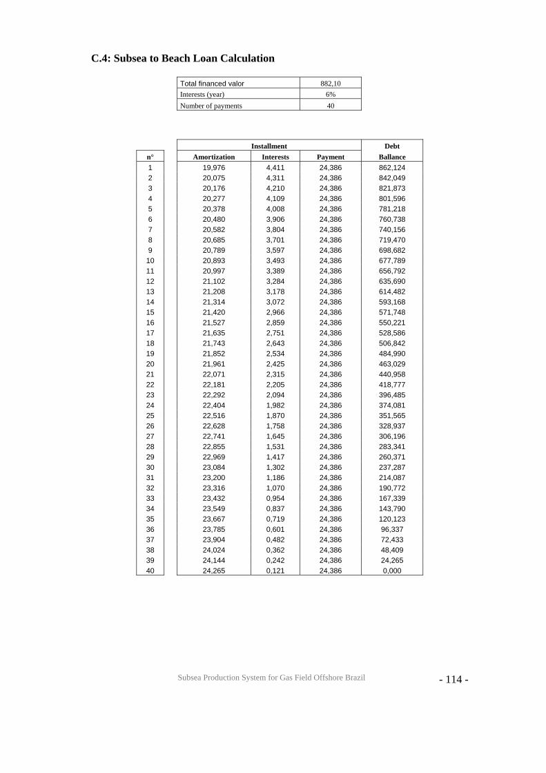
Subsea Production System for Gas Field Offshore Brazil
- 114 -
C.4: Subsea to Beach Loan Calculation
Total financed valor 882,10 Interests (year) 6% Number of payments 40
Installment Debt n° Amortization Interests Payment Ballance 1 19,976 4,411 24,386 862,124 2 20,075 4,311 24,386 842,049 3 20,176 4,210 24,386 821,873 4 20,277 4,109 24,386 801,596 5 20,378 4,008 24,386 781,218 6 20,480 3,906 24,386 760,738 7 20,582 3,804 24,386 740,156 8 20,685 3,701 24,386 719,470 9 20,789 3,597 24,386 698,682
10 20,893 3,493 24,386 677,789 11 20,997 3,389 24,386 656,792 12 21,102 3,284 24,386 635,690 13 21,208 3,178 24,386 614,482 14 21,314 3,072 24,386 593,168 15 21,420 2,966 24,386 571,748 16 21,527 2,859 24,386 550,221 17 21,635 2,751 24,386 528,586 18 21,743 2,643 24,386 506,842 19 21,852 2,534 24,386 484,990 20 21,961 2,425 24,386 463,029 21 22,071 2,315 24,386 440,958 22 22,181 2,205 24,386 418,777 23 22,292 2,094 24,386 396,485 24 22,404 1,982 24,386 374,081 25 22,516 1,870 24,386 351,565 26 22,628 1,758 24,386 328,937 27 22,741 1,645 24,386 306,196 28 22,855 1,531 24,386 283,341 29 22,969 1,417 24,386 260,371 30 23,084 1,302 24,386 237,287 31 23,200 1,186 24,386 214,087 32 23,316 1,070 24,386 190,772 33 23,432 0,954 24,386 167,339 34 23,549 0,837 24,386 143,790 35 23,667 0,719 24,386 120,123 36 23,785 0,601 24,386 96,337 37 23,904 0,482 24,386 72,433 38 24,024 0,362 24,386 48,409 39 24,144 0,242 24,386 24,265 40 24,265 0,121 24,386 0,000
Related Documents