1,2, Yanlin Ge 1,2 1,2,* , Huijun Feng 1,2

entropy

Article

Power and Thermal Efficiency Optimization of an IrreversibleSteady-Flow Lenoir Cycle

Ruibo Wang 1,2, Yanlin Ge 1,2, Lingen Chen 1,2,* , Huijun Feng 1,2 and Zhixiang Wu 1,2

�����������������

Citation: Wang, R.; Ge, Y.; Chen, L.;

Feng, H.; Wu, Z. Power and Thermal

Efficiency Optimization of an

Irreversible Steady-Flow Lenoir

Cycle. Entropy 2021, 23, 425.

https://doi.org/10.3390/e23040425

Academic Editor: Michel Feidt

Received: 15 March 2021

Accepted: 31 March 2021

Published: 2 April 2021

Publisher’s Note: MDPI stays neutral

with regard to jurisdictional claims in

published maps and institutional affil-

iations.

Copyright: © 2021 by the authors.

Licensee MDPI, Basel, Switzerland.

This article is an open access article

distributed under the terms and

conditions of the Creative Commons

Attribution (CC BY) license (https://

creativecommons.org/licenses/by/

4.0/).

1 Institute of Thermal Science and Power Engineering, Wuhan Institute of Technology, Wuhan 430205, China;[email protected] (R.W.); [email protected] (Y.G.); [email protected] (H.F.);[email protected] (Z.W.)

2 School of Mechanical & Electrical Engineering, Wuhan Institute of Technology, Wuhan 430205, China* Correspondence: [email protected]

Abstract: Using finite time thermodynamic theory, an irreversible steady-flow Lenoir cycle modelis established, and expressions of power output and thermal efficiency for the model are derived.Through numerical calculations, with the different fixed total heat conductances (UT) of two heatexchangers, the maximum powers (Pmax), the maximum thermal efficiencies (ηmax), and the corre-sponding optimal heat conductance distribution ratios (uLP(opt)) and (uLη(opt)) are obtained. Theeffects of the internal irreversibility are analyzed. The results show that, when the heat conductancesof the hot- and cold-side heat exchangers are constants, the corresponding power output and thermalefficiency are constant values. When the heat source temperature ratio (τ) and the effectivenesses ofthe heat exchangers increase, the corresponding power output and thermal efficiency increase. Whenthe heat conductance distributions are the optimal values, the characteristic relationships of P− uL

and η − uL are parabolic-like ones. When UT is given, with the increase in τ, the Pmax, ηmax, uLP(opt),and uLη(opt) increase. When τ is given, with the increase in UT , Pmax and ηmax increase, while uLP(opt)and uLη(opt) decrease.

Keywords: finite time thermodynamics; irreversible Lenoir cycle; cycle power; thermal efficiency;heat conductance distribution; performance optimization

1. Introduction

Finite time thermodynamic (FTT) theory [1–4] has been applied to the performanceanalysis and optimization of heat engine (HEG) cycles, and fruitful results have beenachieved for both reciprocating and steady-flow cycle models. For the steady-flow models,FTT was also termed as finite physical dimensions thermodynamics by Feidt [5–10]. Thefamous thermal efficiency formula η = 1−

√TL/TH , where TH and TL are the temperatures

of the heat source and heat sink of a HEG, was derived by Moutier [11] in 1872, Cotterill [12]in 1890, and Novikov [13] and Chambadel [14] in 1957 for steady-flow power plants, whilethe systematical analysis combining thermodynamics with heat transfer for Carnot cyclewas performed by Curzon and Ahlborn [15] in 1975 for reciprocating model, and FTTdevelopment was promoted by Berry’s group [4].

A large number of works have been performed for reciprocating (finite time) mod-els [16–25] by applying FTT. While finite size is the major feature for steady-flow devices,such as closed gas rubine (Brayton cycle) power plants and steam (Rankine cycle) andorganic Rankine cycle power plants, many scholars have performed FTT studies for varioussteady-flow cycles with the power output (POW), thermal efficiency (TEF), exergy effi-ciency, profit rate, and ecological function as the optimization goals, under the conditionsof different losses and heat transfer laws [26–51].

Lenoir [52] first proposed the Lenoir cycle (LC) model in 1860. The simple LC consistsof only three processes of constant-volume endothermic, adiabatic expansion, and constant-pressure exothermic; the LC is also called the triangular cycle. According to the cycle

Entropy 2021, 23, 425. https://doi.org/10.3390/e23040425 https://www.mdpi.com/journal/entropy

Entropy 2021, 23, 425 2 of 11

form, LC can be divided into steady-flow and reciprocating. Georgiou [53] first usedclassical thermodynamics to study the performances of simple, regenerated, and modifiedregenerated steady-flow Lenoir cycles (SFLCs).

Following on from [53], Shen et al. [54] applied FTT theory to optimize the POW andTEF characteristics of the endoreversible SFLC with only the loss of heat resistance, andthey studied the influences of heat source temperature ratio and total heat conductance(HC) on cycle performance. Ahmadi et al. [55] used a genetic algorithm to carry outmultiobjective optimization for endoreversible SFLC, and they obtained the optimal valuesof ecological performance coefficient and thermal economy under different temperatureratios.

In this paper, an irreversible SFLC model will be established on the basis of [54], whilethe cycle performance will be analyzed and optimized with the POW and TEF as objectivefunctions, the optimal HC distributions of hot- and cold-side heat exchangers (HACHEX) ofthe cycle will be studied under different fixed total HCs, and the characteristic relationshipsbetween POW and TEF versus HC distribution are obtained. The effect of the internalirreversibility will be analyzed.

2. Cycle Model

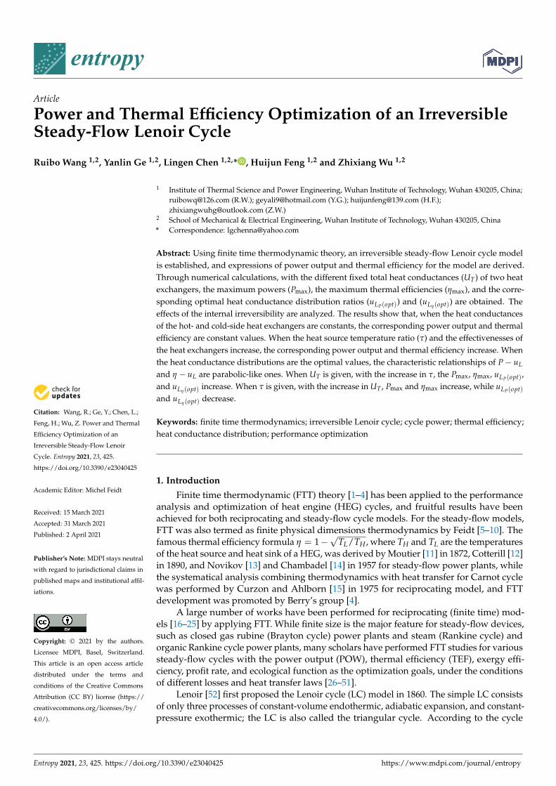
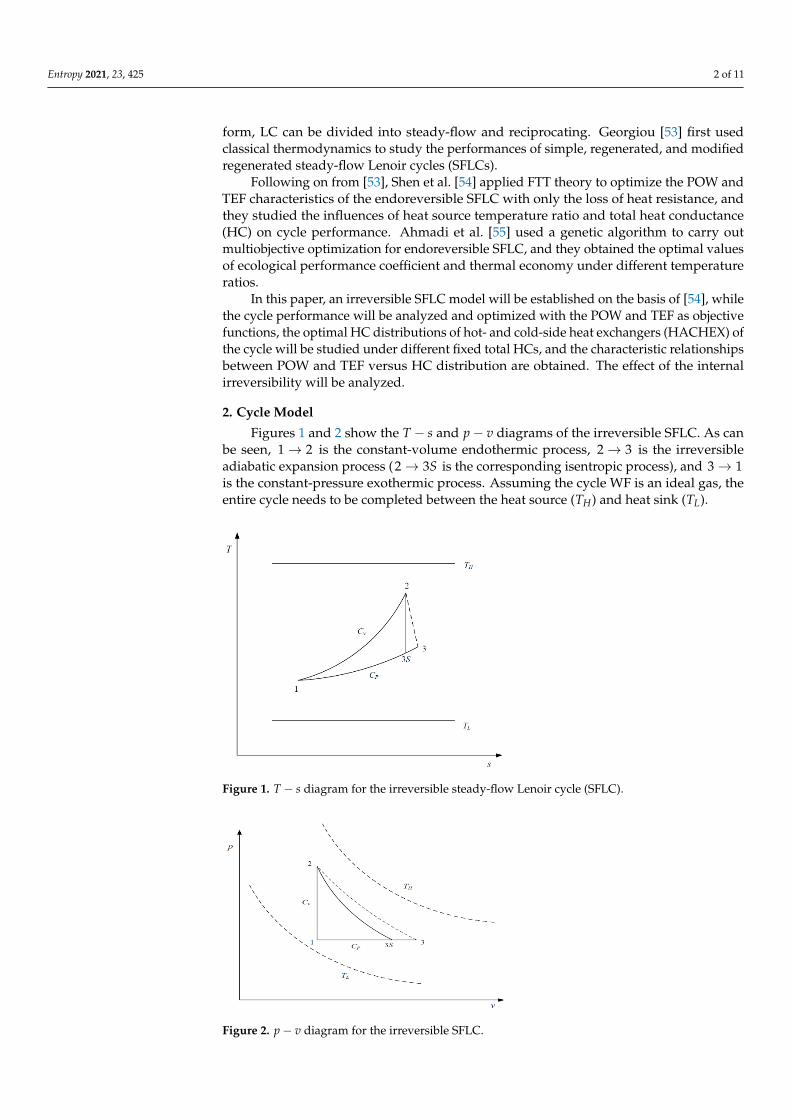
Figures 1 and 2 show the T− s and p− v diagrams of the irreversible SFLC. As canbe seen, 1→ 2 is the constant-volume endothermic process, 2→ 3 is the irreversibleadiabatic expansion process (2→ 3S is the corresponding isentropic process), and 3→ 1is the constant-pressure exothermic process. Assuming the cycle WF is an ideal gas, theentire cycle needs to be completed between the heat source (TH) and heat sink (TL).

Entropy 2021, 23, x FOR PEER REVIEW 2 of 12

Lenoir [52] first proposed the Lenoir cycle (LC) model in 1860. The simple LC consists

of only three processes of constant-volume endothermic, adiabatic expansion, and con-

stant-pressure exothermic; the LC is also called the triangular cycle. According to the cycle

form, LC can be divided into steady-flow and reciprocating. Georgiou [53] first used clas-

sical thermodynamics to study the performances of simple, regenerated, and modified

regenerated steady-flow Lenoir cycles (SFLCs).

Following on from [53], Shen et al. [54] applied FTT theory to optimize the POW and

TEF characteristics of the endoreversible SFLC with only the loss of heat resistance, and

they studied the influences of heat source temperature ratio and total heat conductance

(HC) on cycle performance. Ahmadi et al. [55] used a genetic algorithm to carry out mul-

tiobjective optimization for endoreversible SFLC, and they obtained the optimal values of

ecological performance coefficient and thermal economy under different temperature ra-

tios.

In this paper, an irreversible SFLC model will be established on the basis of [54],

while the cycle performance will be analyzed and optimized with the POW and TEF as

objective functions, the optimal HC distributions of hot- and cold-side heat exchangers

(HACHEX) of the cycle will be studied under different fixed total HCs, and the character-

istic relationships between POW and TEF versus HC distribution are obtained. The effect

of the internal irreversibility will be analyzed.

2. Cycle Model

Figures 1 and 2 show the T s and p v diagrams of the irreversible SFLC. As can

be seen, 1 2 is the constant-volume endothermic process, 2 3 is the irreversible ad-

iabatic expansion process ( 2 3S is the corresponding isentropic process), and 3 1 is

the constant-pressure exothermic process. Assuming the cycle WF is an ideal gas, the en-

tire cycle needs to be completed between the heat source ( HT ) and heat sink ( LT ).

Figure 1. T s diagram for the irreversible steady-flow Lenoir cycle (SFLC). Figure 1. T − s diagram for the irreversible steady-flow Lenoir cycle (SFLC).Entropy 2021, 23, x FOR PEER REVIEW 3 of 12

Figure 2. p v diagram for the irreversible SFLC.

In the actual work of the HEG, there are irreversible losses during compression and

expansion processes; thus, the irreversible expansion efficiency E is defined to describe

the irreversible loss during the expansion process.

2 3

2 3

E

S

T T

T T

, (1)

where iT ( 2,3,3i S ) is the corresponding state point temperature.

Assuming that the heat transfer between the WF and heat reservoir obeys the law of

Newton heat transfer, according to the theory of the heat exchanger (HEX) and the ideal

gas properties, the cycle heat absorbing and heat releasing rates are, respectively,

1 2 1 2 1( ) ( )v H H vQ mC E T T mC T T , (2)

3 1 3 3 1( ) ( )P L L PQ mC E T T mC T T , (3)

where m is the mass flow rate of the WF, vC ( PC ) is the constant-volume (constant-pres-

sure) SH ( =P vC kC , k is the cycle SH ratio), and HE ( LE ) is the effectiveness of hot-side

(cold-side) HEX.

The relationships among the effectivenesses with the corresponding heat transfer

unit numbers ( HN , LN ) and HCs ( HU , LU ) are as follows:

/ ( )H H vN U mC , (4)

/ ( )L L vN U mkC , (5)

1 exp( )H HE N , (6)

1 exp( )L LE N . (7)

3. Analysis and Discussion

3.1. Power and Thermal Efficiency Expressions

According to the second law of thermodynamics, after a cycle process, the total en-

tropy change of the WF is equal to zero; thus, one finds

2 1 3 1ln( / ) ln( / ) 0v P SC T T C T T . (8)

From Equation (8), one obtains

32

1 1

( )kSTT

T T .

(9)

From Equations (2) and (3), one has

Figure 2. p− v diagram for the irreversible SFLC.

Entropy 2021, 23, 425 3 of 11

In the actual work of the HEG, there are irreversible losses during compression andexpansion processes; thus, the irreversible expansion efficiency ηE is defined to describethe irreversible loss during the expansion process.

ηE =T2 − T3

T2 − T3S, (1)

where Ti (i = 2, 3, 3S) is the corresponding state point temperature.Assuming that the heat transfer between the WF and heat reservoir obeys the law of

Newton heat transfer, according to the theory of the heat exchanger (HEX) and the idealgas properties, the cycle heat absorbing and heat releasing rates are, respectively,

.Q1→2 =

.mCvEH(TH − T1) =

.mCv(T2 − T1), (2)

.Q3→1 =

.mCPEL(T3 − TL) =

.mCP(T3 − T1), (3)

where.

m is the mass flow rate of the WF, Cv(CP) is the constant-volume (constant-pressure)SH (CP = kCv, k is the cycle SH ratio), and EH(EL) is the effectiveness of hot-side (cold-side)HEX.

The relationships among the effectivenesses with the corresponding heat transfer unitnumbers (NH , NL) and HCs (UH , UL) are as follows:

NH = UH/(.

mCv), (4)

NL = UL/(.

mkCv), (5)

EH = 1− exp(−NH), (6)

EL = 1− exp(−NL). (7)

3. Analysis and Discussion3.1. Power and Thermal Efficiency Expressions

According to the second law of thermodynamics, after a cycle process, the total entropychange of the WF is equal to zero; thus, one finds

Cv ln(T2/T1)− CP ln(T3S/T1) = 0. (8)

From Equation (8), one obtains

T2

T1= (

T3ST1

)k. (9)

From Equations (2) and (3), one has

T2 = EH(TH − T1) + T1, (10)

T3 = (ELTL − T1)/(EL − 1). (11)

Combining Equations (1), (9), and (10) with Equation (11) yields

T1 =EHTH(ηE − 1) + (T1 − ELTL)/(1− EL)

{(1− EH)(1− ηE) + {[EHTH + (1− EH)T1]/T1}1k ηE}

. (12)

From Equations (2), (3) and (9)–(11), the POW and TEF expressions of the irreversibleSFLC can be obtained as

P =.

Q1→2 −.

Q3→1 =.

mCv[EH(TH − T1)−kEL(T1 − TL)

1− EL], (13)

Entropy 2021, 23, 425 4 of 11

η = P/.

Q1→2 = 1− kEL(T1 − TL)

EH(1− EL)(TH − T1). (14)

When ηE = 1, Equation (12) simplifies to

T1 − ELTL = (1− EL)[EHTH + (1− EH)T1]1k T1

1− 1k . (15)

Equation (15) in this paper is consistent with Equation (15) in [54], where T1 wasobtained for the endoreversible SFLC. Combining Equations (13)–(15) and using the nu-merical solution method, the POW and TEF characteristics of the endoreversible SFLCin [54] can be obtained.

3.2. Case with Given Hot- and Cold-Side HCs

The working cycles of common four-branch HEGs, such as Carnot, Brayton, and Ottoengines, can be roughly divided into four processes: compression, endothermic, expansion,and exothermic. Compared with these common four-stroke cycles, the biggest feature ofthe SFLC is the lack of a gas compression process, presenting a relatively rare three-branchcycle model.

When the hot- and cold-side HCs are constant, it can be seen from Equations (4)–(7)that the effectivenesses of the HACHEX which are directly related to each cycle state pointtemperature will be fixed values; as a result, the POW and TEF will also be fixed values.

3.3. Case with Variable Hot- and Cold-Side HCs When Total HC Is Given

When the HC changes, the POW and TEF of the cycle will also change; therefore, theHC can be optimized and the optimal POW and TEF can be obtained. Assuming the totalHC is a constant,

UL + UH = UT . (16)

Defining the HC distribution ratio as uL = ULUT

(0 < uL < 1), from Equations (4)–(7),the effectivenesses of the HACHEX can be represented as

EH = 1− exp[−(1− uL)UT/(.

mCv)], (17)

EL = 1− exp[−uLUT/(.

mkCv)]. (18)

Combining Equations (12)–(14) and (17) with Equation (18) and using a numericalsolution method, the characteristic relationships between POW and the hot- and cold-sideHC distribution ratio, as well as between TEF and the hot- and cold-side HC distributionratio, can be obtained.

4. Numerical Examples

It is assumed that the working fluid is air. Therefore, its constant-volume specific heatand specific heat ratio are Cv = 0.7165 kJ/(kg·K) and k = 1.4. The turbine efficiency of thegas turbine is about ηE = 0.92 in general. According to the [51–55],

.m = 1.1165 kg/s and

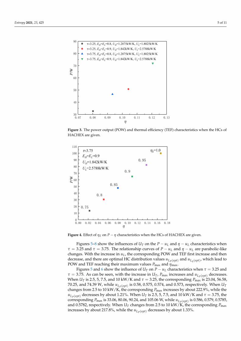
TL = 320 K were set.Figure 3 shows the POW and TEF characteristics when the HCs of the HACHEX and

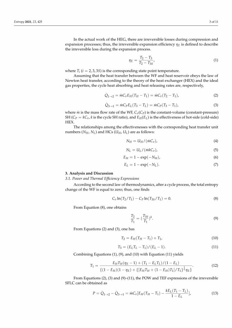
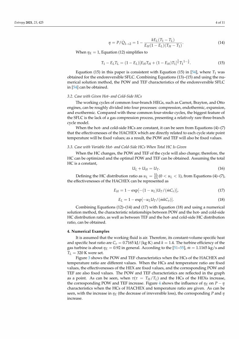
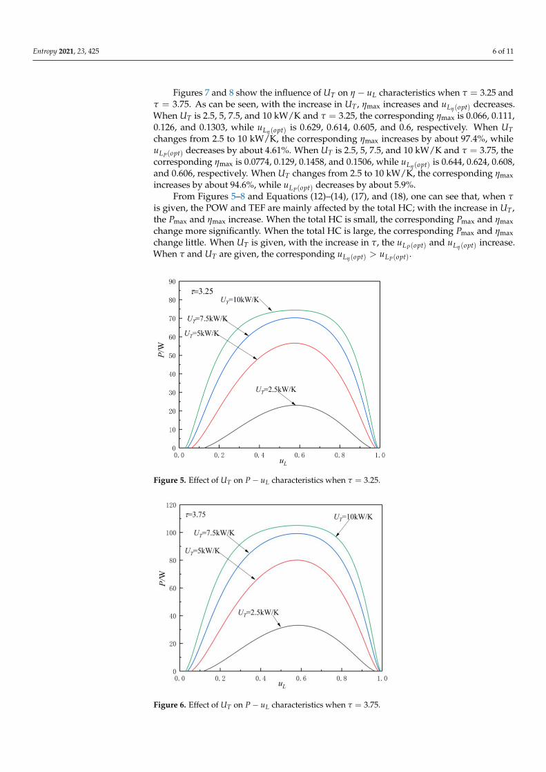
temperature ratio are different values. When the HCs and temperature ratio are fixedvalues, the effectivenesses of the HEX are fixed values, and the corresponding POW andTEF are also fixed values. The POW and TEF characteristics are reflected in the graphas a point. As can be seen, when τ(τ = TH/TL) and the HCs of the HEXs increase,the corresponding POW and TEF increase. Figure 4 shows the influence of ηE on P− ηcharacteristics when the HCs of HACHEX and temperature ratio are given. As can beseen, with the increase in ηE (the decrease of irreversible loss), the corresponding P and ηincrease.

Entropy 2021, 23, 425 5 of 11

Entropy 2021, 23, x FOR PEER REVIEW 5 of 12

4. Numerical Examples

It is assumed that the working fluid is air. Therefore, its constant-volume specific heat

and specific heat ratio are 0.7165kJ / (kg K)vC and 1.4k . The turbine efficiency of the

gas turbine is about =0.92E in general. According to the [51–55], 1.1165kg/ sm and

=320KLT were set.

Figure 3 shows the POW and TEF characteristics when the HCs of the HACHEX and

temperature ratio are different values. When the HCs and temperature ratio are fixed val-

ues, the effectivenesses of the HEX are fixed values, and the corresponding POW and TEF

are also fixed values. The POW and TEF characteristics are reflected in the graph as a

point. As can be seen, when ( = /H LT T ) and the HCs of the HEXs increase, the corre-

sponding POW and TEF increase. Figure 4 shows the influence of E on -P charac-

teristics when the HCs of HACHEX and temperature ratio are given. As can be seen, with

the increase in E (the decrease of irreversible loss), the corresponding P and in-

crease.

Figure 3. The power output (POW) and thermal efficiency (TEF) characteristics when the HCs of

HACHEX are given.

Figure 4. Effect of E on -P characteristics when the HCs of HACHEX are given.

Figure 3. The power output (POW) and thermal efficiency (TEF) characteristics when the HCs ofHACHEX are given.

Entropy 2021, 23, x FOR PEER REVIEW 5 of 12

4. Numerical Examples

It is assumed that the working fluid is air. Therefore, its constant-volume specific heat

and specific heat ratio are 0.7165kJ / (kg K)vC and 1.4k . The turbine efficiency of the

gas turbine is about =0.92E in general. According to the [51–55], 1.1165kg/ sm and

=320KLT were set.

Figure 3 shows the POW and TEF characteristics when the HCs of the HACHEX and

temperature ratio are different values. When the HCs and temperature ratio are fixed val-

ues, the effectivenesses of the HEX are fixed values, and the corresponding POW and TEF

are also fixed values. The POW and TEF characteristics are reflected in the graph as a

point. As can be seen, when ( = /H LT T ) and the HCs of the HEXs increase, the corre-

sponding POW and TEF increase. Figure 4 shows the influence of E on -P charac-

teristics when the HCs of HACHEX and temperature ratio are given. As can be seen, with

the increase in E (the decrease of irreversible loss), the corresponding P and in-

crease.

Figure 3. The power output (POW) and thermal efficiency (TEF) characteristics when the HCs of

HACHEX are given.

Figure 4. Effect of E on -P characteristics when the HCs of HACHEX are given. Figure 4. Effect of ηE on P− η characteristics when the HCs of HACHEX are given.

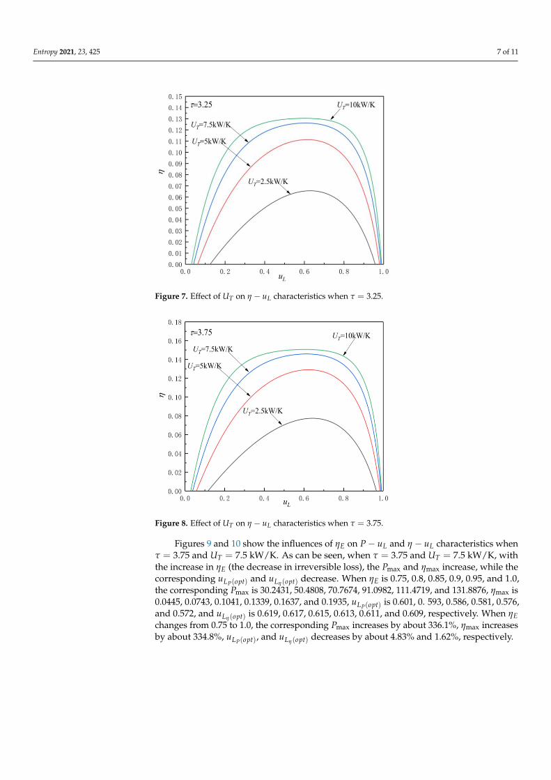
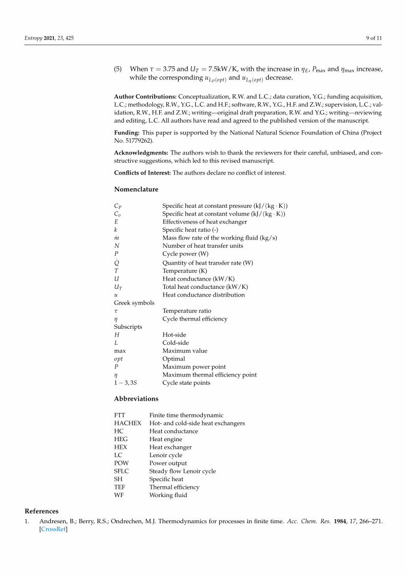
Figures 5–8 show the influences of UT on the P− uL and η − uL characteristics whenτ = 3.25 and τ = 3.75. The relationship curves of P− uL and η − uL are parabolic-likechanges. With the increase in uL, the corresponding POW and TEF first increase and thendecrease, and there are optimal HC distribution values uLP(opt) and uLη(opt), which lead toPOW and TEF reaching their maximum values Pmax and ηmax.

Figures 5 and 6 show the influence of UT on P− uL characteristics when τ = 3.25 andτ = 3.75. As can be seen, with the increase in UT , Pmax increases and uLP(opt) decreases.When UT is 2.5, 5, 7.5, and 10 kW/K and τ = 3.25, the corresponding Pmax is 23.04, 56.58,70.25, and 74.39 W, while uLP(opt) is 0.58, 0.575, 0.574, and 0.573, respectively. When UTchanges from 2.5 to 10 kW/K, the corresponding Pmax increases by about 222.9%, while theuLP(opt) decreases by about 1.21%. When UT is 2.5, 5, 7.5, and 10 kW/K and τ = 3.75, thecorresponding Pmax is 33.06, 80.06, 90.24, and 105.06 W, while uLP(opt) is 0.586, 0.579, 0.5785,and 0.5782, respectively. When UT changes from 2.5 to 10 kW/K, the corresponding Pmaxincreases by about 217.8%, while the uLP(opt) decreases by about 1.33%.

Entropy 2021, 23, 425 6 of 11

Figures 7 and 8 show the influence of UT on η − uL characteristics when τ = 3.25 andτ = 3.75. As can be seen, with the increase in UT , ηmax increases and uLη(opt) decreases.When UT is 2.5, 5, 7.5, and 10 kW/K and τ = 3.25, the corresponding ηmax is 0.066, 0.111,0.126, and 0.1303, while uLη(opt) is 0.629, 0.614, 0.605, and 0.6, respectively. When UTchanges from 2.5 to 10 kW/K, the corresponding ηmax increases by about 97.4%, whileuLP(opt) decreases by about 4.61%. When UT is 2.5, 5, 7.5, and 10 kW/K and τ = 3.75, thecorresponding ηmax is 0.0774, 0.129, 0.1458, and 0.1506, while uLη(opt) is 0.644, 0.624, 0.608,and 0.606, respectively. When UT changes from 2.5 to 10 kW/K, the corresponding ηmaxincreases by about 94.6%, while uLP(opt) decreases by about 5.9%.

From Figures 5–8 and Equations (12)–(14), (17), and (18), one can see that, when τis given, the POW and TEF are mainly affected by the total HC; with the increase in UT ,the Pmax and ηmax increase. When the total HC is small, the corresponding Pmax and ηmaxchange more significantly. When the total HC is large, the corresponding Pmax and ηmaxchange little. When UT is given, with the increase in τ, the uLP(opt) and uLη(opt) increase.When τ and UT are given, the corresponding uLη(opt) > uLP(opt).

Entropy 2021, 23, x FOR PEER REVIEW 6 of 12

Figures 5–8 show the influences of TU on the - LP u and - Lu characteristics when

=3.25 and =3.75 . The relationship curves of - LP u and - Lu are parabolic-like

changes. With the increase in Lu , the corresponding POW and TEF first increase and then

decrease, and there are optimal HC distribution values ( )PL optu and

( )L optu

, which lead to

POW and TEF reaching their maximum values maxP and max .

Figures 5 and 6 show the influence of TU on - LP u characteristics when =3.25

and =3.75 . As can be seen, with the increase in TU , maxP increases and ( )PL optu de-

creases. When TU is 2.5, 5, 7.5, and 10 kW/K and =3.25 , the corresponding maxP is

23.04, 56.58, 70.25, and 74.39 W , while( )PL optu is 0.58, 0.575, 0.574, and 0.573, respectively.

When TU changes from 2.5 to 10 kW/K , the corresponding

maxP increases by about

222.9%, while the ( )PL optu decreases by about 1.21%. When TU is 2.5, 5, 7.5, and 10

kW/K and =3.75 , the corresponding maxP is 33.06, 80.06, 90.24, and 105.06 W, while

( )PL optu is 0.586, 0.579, 0.5785, and 0.5782, respectively. When TU changes from 2.5 to 10

kW/K , the corresponding maxP increases by about 217.8%, while the ( )PL optu decreases

by about 1.33%.

Figures 7 and 8 show the influence of TU on - Lu characteristics when =3.25

and =3.75 . As can be seen, with the increase in TU , max increases and ( )L optu

de-

creases. When TU is 2.5, 5, 7.5, and 10 kW/K and =3.25 , the corresponding max is

0.066, 0.111, 0.126, and 0.1303, while ( )L optu

is 0.629, 0.614, 0.605, and 0.6, respectively.

When TU changes from 2.5 to 10 kW/K , the corresponding max increases by about

97.4%, while ( )PL optu decreases by about 4.61%. When TU is 2.5, 5, 7.5, and 10 kW/K

and =3.75 , the corresponding max is 0.0774, 0.129, 0.1458, and 0.1506, while ( )L optu

is

0.644, 0.624, 0.608, and 0.606, respectively. When TU changes from 2.5 to 10 kW/K , the

corresponding max increases by about 94.6%, while ( )PL optu decreases by about 5.9%.

From Figures 5–8 and Equations (12)–(14), (17), and (18), one can see that, when

is given, the POW and TEF are mainly affected by the total HC; with the increase in TU ,

the maxP and max increase. When the total HC is small, the corresponding maxP and

max change more significantly. When the total HC is large, the corresponding maxP and

max change little. When TU is given, with the increase in , the ( )PL optu and

( )L optu

in-

crease. When and TU are given, the corresponding ( ) ( )PL opt L optu u

.

Figure 5. Effect of UT on P− uL characteristics when τ = 3.25.

Entropy 2021, 23, x FOR PEER REVIEW 7 of 12

Figure 5. Effect of TU on - LP u characteristics when =3.25 .

Figure 6. Effect of TU on - LP u characteristics when =3.75 .

Figure 7. Effect of TU on - Lu characteristics when =3.25 .

Figure 6. Effect of UT on P− uL characteristics when τ = 3.75.

Entropy 2021, 23, 425 7 of 11

Entropy 2021, 23, x FOR PEER REVIEW 7 of 12

Figure 5. Effect of TU on - LP u characteristics when =3.25 .

Figure 6. Effect of TU on - LP u characteristics when =3.75 .

Figure 7. Effect of TU on - Lu characteristics when =3.25 . Figure 7. Effect of UT on η − uL characteristics when τ = 3.25.Entropy 2021, 23, x FOR PEER REVIEW 8 of 12

Figure 8. Effect of TU on - Lu characteristics when =3.75 .

Figures 9 and 10 show the influences of E on - LP u and - Lu characteristics when

=3.75 and 7.5kW/KTU . As can be seen, when =3.75 and 7.5kW/KTU , with the

increase in E (the decrease in irreversible loss), the maxP and max increase, while the

corresponding ( )PL optu and

( )L optu

decrease. When E is 0.75, 0.8, 0.85, 0.9, 0.95, and 1.0,

the corresponding maxP is 30.2431, 50.4808, 70.7674, 91.0982, 111.4719, and 131.8876,

max

is 0.0445, 0.0743, 0.1041, 0.1339, 0.1637, and 0.1935, ( )PL optu is 0.601, 0. 593, 0.586, 0.581,

0.576, and 0.572, and ( )L optu

is 0.619, 0.617, 0.615, 0.613, 0.611, and 0.609, respectively.

When E changes from 0.75 to 1.0, the corresponding maxP increases by about 336.1%,

max increases by about 334.8%, ( )PL optu , and

( )L optu

decreases by about 4.83% and 1.62%,

respectively.

Figure 9. Effect of E on - LP u characteristics.

Figure 8. Effect of UT on η − uL characteristics when τ = 3.75.

Figures 9 and 10 show the influences of ηE on P− uL and η − uL characteristics whenτ = 3.75 and UT = 7.5 kW/K. As can be seen, when τ = 3.75 and UT = 7.5 kW/K, withthe increase in ηE (the decrease in irreversible loss), the Pmax and ηmax increase, while thecorresponding uLP(opt) and uLη(opt) decrease. When ηE is 0.75, 0.8, 0.85, 0.9, 0.95, and 1.0,the corresponding Pmax is 30.2431, 50.4808, 70.7674, 91.0982, 111.4719, and 131.8876, ηmax is0.0445, 0.0743, 0.1041, 0.1339, 0.1637, and 0.1935, uLP(opt) is 0.601, 0. 593, 0.586, 0.581, 0.576,and 0.572, and uLη(opt) is 0.619, 0.617, 0.615, 0.613, 0.611, and 0.609, respectively. When ηEchanges from 0.75 to 1.0, the corresponding Pmax increases by about 336.1%, ηmax increasesby about 334.8%, uLP(opt), and uLη(opt) decreases by about 4.83% and 1.62%, respectively.

Entropy 2021, 23, 425 8 of 11

Entropy 2021, 23, x FOR PEER REVIEW 8 of 12

Figure 8. Effect of TU on - Lu characteristics when =3.75 .

Figures 9 and 10 show the influences of E on - LP u and - Lu characteristics when

=3.75 and 7.5kW/KTU . As can be seen, when =3.75 and 7.5kW/KTU , with the

increase in E (the decrease in irreversible loss), the maxP and max increase, while the

corresponding ( )PL optu and

( )L optu

decrease. When E is 0.75, 0.8, 0.85, 0.9, 0.95, and 1.0,

the corresponding maxP is 30.2431, 50.4808, 70.7674, 91.0982, 111.4719, and 131.8876,

max

is 0.0445, 0.0743, 0.1041, 0.1339, 0.1637, and 0.1935, ( )PL optu is 0.601, 0. 593, 0.586, 0.581,

0.576, and 0.572, and ( )L optu

is 0.619, 0.617, 0.615, 0.613, 0.611, and 0.609, respectively.

When E changes from 0.75 to 1.0, the corresponding maxP increases by about 336.1%,

max increases by about 334.8%, ( )PL optu , and

( )L optu

decreases by about 4.83% and 1.62%,

respectively.

Figure 9. Effect of E on - LP u characteristics. Figure 9. Effect of ηE on P− uL characteristics.Entropy 2021, 23, x FOR PEER REVIEW 9 of 12

Figure 10. Effect of E on - Lu characteristics.

5. Conclusions

In this paper, an irreversible SFLC model is established on the basis of [54], while the

POW and TEF characteristics of the irreversible SFLC were studied using FTT theory, and

the influences of , TU and E on maxP , max , ( )PL optu , and

( )L optu

were analyzed. The

main conclusions are as follows:

(1) When the HCs are constants, the corresponding POW and TEF are fixed values. When

and the HCs of the HEXs increase, the corresponding POW and TEF increase.

When and HCs of the HEXs are constants, with the increase in E (the decrease

in irreversible loss), the corresponding P and increase.

(2) When the distribution of HCs can be optimized, the relationships of - LP u and - Lu

are parabolic-like ones.

(3) When TU is given, with the increase in , maxP , max , ( )PL optu , and

( )L optu

increase.

(4) When is given, with the increase in TU , maxP and max increase, while ( )PL optu

and ( )L optu

decrease. When and TU are given, the corresponding

( )L optu

is big-

ger than ( )PL optu .

(5) When =3.75 and 7.5kW/KTU , with the increase in E , maxP and max increase,

while the corresponding ( )PL optu and

( )L optu

decrease.

Author Contributions: Conceptualization, R.W. and L.C.; data curation, Y.G.; funding acquisition,

L.C.; methodology, R.W., Y.G., L.C. and H.F.; software, R.W., Y.G., H.F. and Z.W.; supervision, L.C.;

validation, R.W., H.F. and Z.W.; writing—original draft preparation, R.W. and Y.G.; writing—re-

viewing and editing, L.C. All authors have read and agreed to the published version of the manu-

script.

Funding: This paper is supported by the National Natural Science Foundation of China (Project No.

51779262).

Acknowledgments: The authors wish to thank the reviewers for their careful, unbiased, and con-

structive suggestions, which led to this revised manuscript.

Conflicts of Interest: The authors declare no conflicts of interest.

Nomenclature

PC Specific heat at constant pressure ( kJ/ (kg K) )

Figure 10. Effect of ηE on η − uL characteristics.

5. Conclusions

In this paper, an irreversible SFLC model is established on the basis of [54], whilethe POW and TEF characteristics of the irreversible SFLC were studied using FTT theory,and the influences of τ, UT and ηE on Pmax, ηmax, uLP(opt), and uLη(opt) were analyzed. Themain conclusions are as follows:

(1) When the HCs are constants, the corresponding POW and TEF are fixed values.When τ and the HCs of the HEXs increase, the corresponding POW and TEF increase.When τ and HCs of the HEXs are constants, with the increase in ηE (the decrease inirreversible loss), the corresponding P and η increase.

(2) When the distribution of HCs can be optimized, the relationships of P− uL and η− uLare parabolic-like ones.

(3) When UT is given, with the increase in τ, Pmax, ηmax, uLP(opt), and uLη(opt) increase.(4) When τ is given, with the increase in UT , Pmax and ηmax increase, while uLP(opt) and

uLη(opt) decrease. When τ and UT are given, the corresponding uLη(opt) is bigger thanuLP(opt).

Entropy 2021, 23, 425 9 of 11

(5) When τ = 3.75 and UT = 7.5kW/K, with the increase in ηE, Pmax and ηmax increase,while the corresponding uLP(opt) and uLη(opt) decrease.

Author Contributions: Conceptualization, R.W. and L.C.; data curation, Y.G.; funding acquisition,L.C.; methodology, R.W., Y.G., L.C. and H.F.; software, R.W., Y.G., H.F. and Z.W.; supervision, L.C.; val-idation, R.W., H.F. and Z.W.; writing—original draft preparation, R.W. and Y.G.; writing—reviewingand editing, L.C. All authors have read and agreed to the published version of the manuscript.

Funding: This paper is supported by the National Natural Science Foundation of China (ProjectNo. 51779262).

Acknowledgments: The authors wish to thank the reviewers for their careful, unbiased, and con-structive suggestions, which led to this revised manuscript.

Conflicts of Interest: The authors declare no conflict of interest.

Nomenclature

CP Specific heat at constant pressure (kJ/(kg ·K))Cv Specific heat at constant volume (kJ/(kg ·K))E Effectiveness of heat exchangerk Specific heat ratio (-).

m Mass flow rate of the working fluid (kg/s)N Number of heat transfer unitsP Cycle power (W).

Q Quantity of heat transfer rate (W)T Temperature (K)U Heat conductance (kW/K)UT Total heat conductance (kW/K)u Heat conductance distributionGreek symbolsτ Temperature ratioη Cycle thermal efficiencySubscriptsH Hot-sideL Cold-sidemax Maximum valueopt OptimalP Maximum power pointη Maximum thermal efficiency point1− 3, 3S Cycle state points

Abbreviations

FTT Finite time thermodynamicHACHEX Hot- and cold-side heat exchangersHC Heat conductanceHEG Heat engineHEX Heat exchangerLC Lenoir cyclePOW Power outputSFLC Steady flow Lenoir cycleSH Specific heatTEF Thermal efficiencyWF Working fluid

References1. Andresen, B.; Berry, R.S.; Ondrechen, M.J. Thermodynamics for processes in finite time. Acc. Chem. Res. 1984, 17, 266–271.

[CrossRef]

Entropy 2021, 23, 425 10 of 11

2. Andresen, B. Current trends in finite-time thermodynamics. Angew. Chem. Int. Ed. 2011, 50, 2690–2704. [CrossRef]3. Feidt, M. The history and perspectives of efficiency at maximum power of the Carnot engine. Entropy 2017, 19, 369. [CrossRef]4. Berry, R.S.; Salamon, P.; Andresen, B. How it all began. Entropy 2020, 22, 908. [CrossRef] [PubMed]5. Feidt, M. Finite Physical Dimensions Optimal Thermodynamics 1. Fundamental; ISTE Press and Elsevier: London, UK, 2017.6. Feidt, M. Finite Physical Dimensions Optimal Thermodynamics 2. Complex. Systems; ISTE Press and Elsevier: London, UK, 2018.7. Blaise, M.; Feidt, M.; Maillet, D. Influence of the working fluid properties on optimized power of an irreversible finite dimensions

Carnot engine. Energy Convers. Manag. 2018, 163, 444–456. [CrossRef]8. Feidt, M.; Costea, M. From finite time to finite physical dimensions thermodynamics: The Carnot engine and Onsager’s relations

revisited. J. Non-Equilib. Thermodyn. 2018, 43, 151–162. [CrossRef]9. Dumitrascu, G.; Feidt, M.; Popescu, A.; Grigorean, S. Endoreversible trigeneration cycle design based on finite physical dimensions

thermodynamics. Energies 2019, 12, 3165.10. Feidt, M.; Costea, M.; Feidt, R.; Danel, Q.; Périlhon, C. New criteria to characterize the waste heat recovery. Energies 2020, 13, 789.

[CrossRef]11. Moutier, J. Éléments de Thermodynamique; Gautier-Villars: Paris, France, 1872.12. Cotterill, J.H. Steam Engines, 2nd ed.; E & F.N. Spon: London, UK, 1890.13. Novikov, I.I. The efficiency of atomic power stations (A review). J. Nucl. Energy 1957, 7, 125–128. [CrossRef]14. Chambadal, P. Les Centrales Nucleaires; Armand Colin: Paris, France, 1957; pp. 41–58.15. Curzon, F.L.; Ahlborn, B. Efficiency of a Carnot engine at maximum power output. Am. J. Phys. 1975, 43, 22–24. [CrossRef]16. Hoffman, K.H.; Burzler, J.; Fischer, A.; Schaller, M.; Schubert, S. Optimal process paths for endoreversible systems. J. Non-Equilib.

Thermodyn. 2003, 28, 233–268. [CrossRef]17. Zaeva, M.A.; Tsirlin, A.M.; Didina, O.V. Finite time thermodynamics: Realizability domain of heat to work converters.

J. Non-Equilib. Thermodyn. 2019, 44, 181–191. [CrossRef]18. Masser, R.; Hoffmann, K.H. Endoreversible modeling of a hydraulic recuperation system. Entropy 2020, 22, 383. [CrossRef]19. Masser, R.; Khodja, A.; Scheunert, M.; Schwalbe, K.; Fischer, A.; Paul, R.; Hoffmann, K.H. Optimized piston motion for an

alpha-type Stirling engine. Entropy 2020, 22, 700. [CrossRef]20. Muschik, W.; Hoffmann, K.H. Modeling, simulation, and reconstruction of 2-reservoir heat-to-power processes in finite-time

thermodynamics. Entropy 2020, 22, 997. [CrossRef]21. Andresen, B.; Essex, C. Thermodynamics at very long time and space scales. Entropy 2020, 22, 1090. [CrossRef]22. Scheunert, M.; Masser, R.; Khodja, A.; Paul, R.; Schwalbe, K.; Fischer, A.; Hoffmann, K.H. Power-optimized sinusoidal piston

motion and its performance gain for an Alpha-type Stirling engine with limited regeneration. Energies 2020, 13, 4564. [CrossRef]23. Chen, L.G.; Feng, H.J.; Ge, Y.L. Maximum energy output chemical pump configuration with an infinite-low- and a finite-high-

chemical potential mass reservoirs. Energy Convers. Manag. 2020, 223, 113261. [CrossRef]24. Qi, C.Z.; Ding, Z.M.; Chen, L.G.; Ge, Y.L.; Feng, H.J. Modeling and performance optimization of an irreversible two-stage

combined thermal Brownian heat engine. Entropy 2021, 23, 419. [CrossRef]25. Chen, L.G.; Meng, Z.W.; Ge, Y.L.; Wu, F. Performance analysis and optimization for irreversible combined Carnot heat engine

working with ideal quantum gases. Entropy 2021, 23. in press.26. Bejan, A. Theory of heat transfer-irreversible power plant. Int. J. Heat Mass Transf. 1988, 31, 1211–1219. [CrossRef]27. Morisaki, T.; Ikegami, Y. Maximum power of a multistage Rankine cycle in low-grade thermal energy conversion. Appl. Therm.

Eng. 2014, 69, 78–85. [CrossRef]28. Sadatsakkak, S.A.; Ahmadi, M.H.; Ahmadi, M.A. Thermodynamic and thermo-economic analysis and optimization of an

irreversible regenerative closed Brayton cycle. Energy Convers. Manag. 2015, 94, 124–129. [CrossRef]29. Yasunaga, T.; Ikegami, Y. Application of finite time thermodynamics for evaluation method of heat engines. Energy Proc. 2017,

129, 995–1001. [CrossRef]30. Yasunaga, T.; Fontaine, K.; Morisaki, T.; Ikegami, Y. Performance evaluation of heat exchangers for application to ocean thermal

energy conversion system. Ocean Therm. Energy Convers. 2017, 22, 65–75.31. Yasunaga, T.; Noguchi, T.; Morisaki, T.; Ikegami, Y. Basic heat exchanger performance evaluation method on OTEC. J. Mar. Sci.

Eng. 2018, 6, 32. [CrossRef]32. Fontaine, K.; Yasunaga, T.; Ikegami, Y. OTEC maximum net power output using Carnot cycle and application to simplify heat

exchanger selection. Entropy 2019, 21, 1143. [CrossRef]33. Fawal, S.; Kodal, A. Comparative performance analysis of various optimization functions for an irreversible Brayton cycle

applicable to turbojet engines. Energy Convers. Manag. 2019, 199, 111976. [CrossRef]34. Yasunaga, T.; Ikegami, Y. Finite-time thermodynamic model for evaluating heat engines in ocean thermal energy conversion.

Entropy 2020, 22, 211. [CrossRef]35. Yu, X.F.; Wang, C.; Yu, D.R. Minimization of entropy generation of a closed Brayton cycle based precooling-compression system

for advanced hypersonic airbreathing engine. Energy Convers. Manag. 2020, 209, 112548. [CrossRef]36. Arora, R.; Arora, R. Thermodynamic optimization of an irreversible regenerated Brayton heat engine using modified ecological

criteria. J. Therm. Eng. 2020, 6, 28–42. [CrossRef]37. Liu, H.T.; Zhai, R.R.; Patchigolla, K.; Turner, P.; Yang, Y.P. Analysis of integration method in multi-heat-source power generation

systems based on finite-time thermodynamics. Energy Convers. Manag. 2020, 220, 113069. [CrossRef]

Entropy 2021, 23, 425 11 of 11

38. Gonca, G.; Sahin, B.; Cakir, M. Performance assessment of a modified power generating cycle based on effective ecological powerdensity and performance coefficient. Int. J. Exergy 2020, 33, 153–164. [CrossRef]

39. Karakurt, A.S.; Bashan, V.; Ust, Y. Comparative maximum power density analysis of a supercritical CO2 Brayton power cycle.J. Therm. Eng. 2020, 6, 50–57. [CrossRef]

40. Ahmadi, M.H.; Dehghani, S.; Mohammadi, A.H.; Feidt, M.; Barranco-Jimenez, M.A. Optimal design of a solar driven heat enginebased on thermal and thermo-economic criteria. Energy Convers. Manag. 2013, 75, 635–642. [CrossRef]

41. Ahmadi, M.H.; Mohammadi, A.H.; Dehghani, S.; Barranco-Jimenez, M.A. Multi-objective thermodynamic-based optimization ofoutput power of Solar Dish-Stirling engine by implementing an evolutionary algorithm. Energy Convers. Manag. 2013, 75, 438–445.[CrossRef]

42. Ahmadi, M.H.; Ahmadi, M.A.; Mohammadi, A.H.; Feidt, M.; Pourkiaei, S.M. Multi-objective optimization of an irreversibleStirling cryogenic refrigerator cycle. Energy Convers. Manag. 2014, 82, 351–360. [CrossRef]

43. Ahmadi, M.H.; Ahmadi, M.A.; Mehrpooya, M.; Hosseinzade, H.; Feidt, M. Thermodynamic and thermo-economic analysisand optimization of performance of irreversible four-temperature-level absorption refrigeration. Energy Convers. Manag. 2014,88, 1051–1059. [CrossRef]

44. Ahmadi, M.H.; Ahmadi, M.A. Thermodynamic analysis and optimization of an irreversible Ericsson cryogenic refrigerator cycle.Energy Convers. Manag. 2015, 89, 147–155. [CrossRef]

45. Jokar, M.A.; Ahmadi, M.H.; Sharifpur, M.; Meyer, J.P.; Pourfayaz, F.; Ming, T.Z. Thermodynamic evaluation and multi-objectiveoptimization of molten carbonate fuel cell-supercritical CO2 Brayton cycle hybrid system. Energy Convers. Manag. 2017,153, 538–556. [CrossRef]

46. Han, Z.H.; Mei, Z.K.; Li, P. Multi-objective optimization and sensitivity analysis of an organic Rankine cycle coupled with aone-dimensional radial-inflow turbine efficiency prediction model. Energy Convers. Manag. 2018, 166, 37–47. [CrossRef]

47. Ghasemkhani, A.; Farahat, S.; Naserian, M.M. Multi-objective optimization and decision making of endoreversible combinedcycles with consideration of different heat exchangers by finite time thermodynamics. Energy Convers. Manag. 2018, 171, 1052–1062.[CrossRef]

48. Ahmadi, M.H.; Jokar, M.A.; Ming, T.Z.; Feidt, M.; Pourfayaz, F.; Astaraei, F.R. Multi-objective performance optimization ofirreversible molten carbonate fuel cell–Braysson heat engine and thermodynamic analysis with ecological objective approach.Energy 2018, 144, 707–722. [CrossRef]

49. Tierney, M. Minimum exergy destruction from endoreversible and finite-time thermodynamics machines and their concomitantindirect energy. Energy 2020, 197, 117184. [CrossRef]

50. Yang, H.; Yang, C.X. Derivation and comparison of thermodynamic characteristics of endoreversible aircraft environmentalcontrol systems. Appl. Therm. Eng. 2020, 180, 115811. [CrossRef]

51. Tang, C.Q.; Chen, L.G.; Feng, H.J.; Ge, Y.L. Four-objective optimization for an irreversible closed modified simple Brayton cycle.Entropy 2021, 23, 282. [CrossRef] [PubMed]

52. Lichty, C. Combustion Engine Processes; McGraw-Hill: New York, NY, USA, 1967.53. Georgiou, D.P. Useful work and the thermal efficiency in the ideal Lenoir with regenerative preheating. J. Appl. Phys. 2008,

88, 5981–5986. [CrossRef]54. Shen, X.; Chen, L.G.; Ge, Y.L.; Sun, F.R. Finite-time thermodynamic analysis for endoreversible Lenoir cycle coupled to constant-

temperature heat reservoirs. Int. J. Energy Environ. 2017, 8, 272–278.55. Ahmadi, M.H.; Nazari, M.A.; Feidt, M. Thermodynamic analysis and multi-objective optimisation of endoreversible Lenoir heat

engine cycle based on the thermo-economic performance criterion. Int. J. Ambient Energy 2019, 40, 600–609. [CrossRef]