1 Weakly Supervised Top-down Salient Object … Weakly Supervised Top-down Salient Object Detection Hisham Cholakkal, Jubin Johnson, and Deepu Rajan Abstract—Top-down saliency models

1

Weakly Supervised Top-down Salient ObjectDetection

Hisham Cholakkal, Jubin Johnson, and Deepu Rajan

Abstract—Top-down saliency models produce a probability map that peaks at target locations specified by a task/goal such as objectdetection. They are usually trained in a fully supervised setting involving pixel-level annotations of objects. We propose a weaklysupervised top-down saliency framework using only binary labels that indicate the presence/absence of an object in an image. First,the probabilistic contribution of each image region to the confidence of a CNN-based image classifier is computed through abacktracking strategy to produce top-down saliency. From a set of saliency maps of an image produced by fast bottom-up saliencyapproaches, we select the best saliency map suitable for the top-down task. The selected bottom-up saliency map is combined with thetop-down saliency map. Features having high combined saliency are used to train a linear SVM classifier to estimate feature saliency.This is integrated with combined saliency and further refined through a multi-scale superpixel-averaging of saliency map. We evaluatethe performance of the proposed weakly supervised top-down saliency against fully supervised approaches and achievestate-of-the-art performance. Experiments are carried out on seven challenging datasets and quantitative results are compared with 36closely related approaches across 4 different applications.

Index Terms—Top-down saliency, salient object detection, weakly supervised training, object segmentation, semantic segmentation,object localization, object detection, CNN image classifier.

F

1 INTRODUCTION

T HE human visual system has the ability to zero-in rapidly ontosalient regions in an image. Recently, there has been much

interest among computer vision researchers to model this processknown as visual saliency, which is attributed to the phenomenonof visual attention. It is beneficial in applications such as objectdetection/segmentation [1], [2], image retargeting [3] etc., sinceidentification of salient regions reduces the search space for suchhigh-level tasks. Salient regions in an image are indicated by aprobability map called the saliency map. Fig. 1 shows saliencymaps in the form of heat maps, where red indicates higher saliency.

In many instances, the salient region corresponds to a specificobject in an image, in which case salient object detection becomesa more apt term, wherein pixels belonging to a salient object areassigned high saliency values. Broadly, there are two approachesto salient object detection: bottom-up (BU) [4] and top-down (TD)[5]. The feature contrast at a location plays the central role in BUsalient object detection, with no regard to the semantic contentsof the scene, although high-level concepts like faces have beenused in conjunction with visual cues like color and shape [6]. Theassumption that the salient object ‘pops out’ does not hold whenthere is little or no contrast between the object and the background.Furthermore, the notion of a salient object is not well-defined inBU models as seen in Fig. 1 (b, c, d) where recent methods [7],[4] and [8] show the potted plant in the background as salient to auser searching for the cat.

TD salient object detection is task-oriented and utilizes priorknowledge about the object class. For example, in semanticsegmentation [9], a pixel is assigned to a particular object class,and a saliency map that aids in this segmentation must invariablybe generated by a top-down approach. Fig. 1(e, f, g, h) show the

• H. Cholakkal, J. Johnson, and D. Rajan are with the School of ComputerScience and Engineering, Nanyang Technological University, Singapore,639798. E-mail: hisham002, jubin001, [email protected].

saliency maps produced by the proposed method for person, cat,sofa and potted plant categories, respectively. TD saliency is alsoviewed as a focus-of-attention mechanism by which BU salientpoints that are unlikely to be part of the object are pruned [10].

Most methods for TD saliency detection learn object classes ina fully supervised manner using pixel-level labeling of objects [5],[11], [12]. Weakly supervised learning (WSL) alleviates the needfor user-intensive annotation by utilizing only class labels forimages. Moosmann et al. [13] propose a weakly supervised TDsaliency method for image classification that employs iterativerefinement of object hypothesis on a training image. Our methoddoes not require any iterations, yet achieves state-of-the-art resultscompared to even fully supervised approaches [5], [14]. Wefirst train a convolutional neural network (CNN) image classifierusing image-level representation of CNN features, that gives aconfidence score on the presence of an object in an image. Theprobabilistic contribution of each discriminative feature to thisconfidence score is represented in a TD saliency map, which iscombined with a BU saliency map that is selected from severalcandidate BU maps through a novel selection strategy. Next, thesaliency of each feature is separately evaluated using a dedicatedfeature classifier, as a means to assign non-zero saliency valuesto features from non-discriminative object regions, based on theirdissimilarity with the background features. Saliency inference at apixel involves combining the image classifier-based saliency mapand the feature classifier-based saliency map.

A preliminary version of this paper was presented at CVPR2016 [15]. The current version is revised with the following mod-ifications: (i) sparse codes of SIFT features in [15] are replacedwith CNN features; (ii) for a given task, a saliency-weighted max-pooling strategy is proposed to select a BU saliency map amongseveral candidates, which is combined with TD saliency map; (iii)since CNN features span larger spatial neighborhood comparedto SIFT features, contextual saliency in [15] is replaced with

arX

iv:1

611.

0534

5v2

[cs

.CV

] 1

7 N

ov 2

016

2

(a) (b) (c) (d)

(e) (f) (g) (h)

Fig. 1. Comparison of proposed top-down salient object detectionwith bottom-up methods. (a) Input image, bottom-up saliency maps of(b)MB [7], (c) MST [4], and (d) HC [8]; proposed top-down saliency mapsfor (e) person (f) cat (g) sofa and (h) potted plant categories.

CNN feature saliency; (iv) multi-scale averaging of saliency valueswithin each superpixel is carried out to improve accuracy alongobject boundaries. These modifications lead not only to betterperformance than [15], but also with recent fully supervised TDapproaches as shown in Fig. 2. Besides illustrating the accuracyof saliency maps produced by the proposed method, we alsodemonstrate the usefulness of our TD salient object detection forweakly supervised applications in semantic segmentation, objectsegmentation, object localization and object detection.

2 RELATED WORK

We review related work in top-down saliency and relevant appli-cations of CNN under weak supervision.

2.1 Top-down saliency frameworksKanan et al. [16] proposed a TD saliency approach which usesobject appearance in conjunction with a location prior. Ineffec-tiveness of this prior largely affects the accuracy based on theposition of the object within the image. Closer to our framework,Yang and Yang [5] proposed a fully supervised TD saliencymodel that jointly learns a conditional random field (CRF) anddictionary using sparse codes of SIFT features as latent variables.The inability to discriminate between objects having similar parts(e.g. wheels of car and motorbike) causes a large number of falsedetections. Kocak et al. [11] improved upon this by replacingSIFT features with the first and second order statistics of color,edge orientation and pixel location within a superpixel, alongwith objectness [17]. Although this improved the accuracy indistinguishing objects from background, it failed to discriminatebetween object categories, causing large number of false detec-tions if the test image contained objects from other categories, asshown in Fig. 2 (b). Blocking artifacts are also observed in thesaliency map at the superpixel boundaries because the superpixelsare extracted on a single scale alone. Khan and Tappen [18] usedlabel and location-dependent smoothness constraint in a sparsecode formulation to produce a smooth saliency map comparedto conventional sparse coding, but with additional computational

cost. A joint framework for image classification and TD saliencyis proposed in [19].

Zhu et al. [20] proposed a contextual-pooling based approachwhere LLC [21] codes of SIFT features are max-pooled in alocal neighborhood followed by log-linear model learning. Byreplacing LLC codes with locality-constrained contextual sparsecoding (LCCSC), Cholakkal et al. [12] improved on [20] witha carefully chosen category-specific dictionary learned from theannotated object area. Discriminative models [10], [22], [23] oftenrepresent a few patches on the object as salient and not the entireobject. Hence, such models end up with low recall rates comparedto [11], [24]. In [23], the task of image classification is improvedusing discriminative spatial saliency to weight visual features.

Recently, a fully supervised, CNN-based TD saliency methodwas proposed that utilized visual association of query images withmultiple object exemplars [14]. They followed a two-stage deepmodel where the first stage learnt object-to-object association andthe second stage learnt object-to-background discrimination. Eachpatch, extracted using a sliding window, is resized to 224 × 224and input separately to the CNN. There are approximately 500patches in an image of size 500 × 400, resulting in 500 forwardpasses through the network. Training the model required morethan a week on a GPU. Our approach needs only one forwardpass to extract CNN features for the entire image, which reducesthe computation time significantly. It is still able to produce bettersaliency maps (Fig. 2 (f)) compared to [14] (Fig. 2 (e)). CNN-based saliency approaches [25], [26], [27], [28] learn category-independent salient features [29] from a large number of fully an-notated training images [8]. Training or fine-tuning these saliencymodels [26], [28] took multiple days, even after initializing theirmodels with convolutional filter weights pre-trained for imageclassification on ImageNet [30].

The use of weak supervision in TD saliency has largely beenleft unexamined. Gao et al. [10] used a weakly supervised set-ting where bottom-up features are combined with discriminativefeatures that maximize the mutual information to the categorylabel. Higher saliency values are assigned only to the featureswhich are discriminative for a category in an image classificationtask, limiting its use in applications such as object segmentation,where all pixels of the object need to be identified accurately.In [13], a joint framework using classifier and TD saliency isused for object categorization by sampling representative windowscontaining the object. Their iterative strategy leads to inaccuratesaliency estimation if the initialized windows do not contain theobject.

2.2 CNN-based weakly supervised frameworks

Recently, CNN has been used in a number of weakly supervisedobject localization approaches [31], [32], [33], [34]. Multiple-instance learning is applied on CNN features in [33]. In [31],image regions are masked out to identify regions causing maximalactivation. The outputs of CNN on multiple overlapping patchesare utilized for object localization in [34]. All these approachesneed multiple forward passes on a network to localize objects,which makes them computationally less efficient. Oquab et al. [32]applied global max-pooling to localize a point on objects. Globalmax-pooling is replaced by average pooling in [35] to help identifythe full extent of the object as well. The underlying assumption isthat the loss for average pooling enables the network to identifydiscriminative object regions. However, the spatial information is

3

(a) (b) (c) (d) (e) (f)

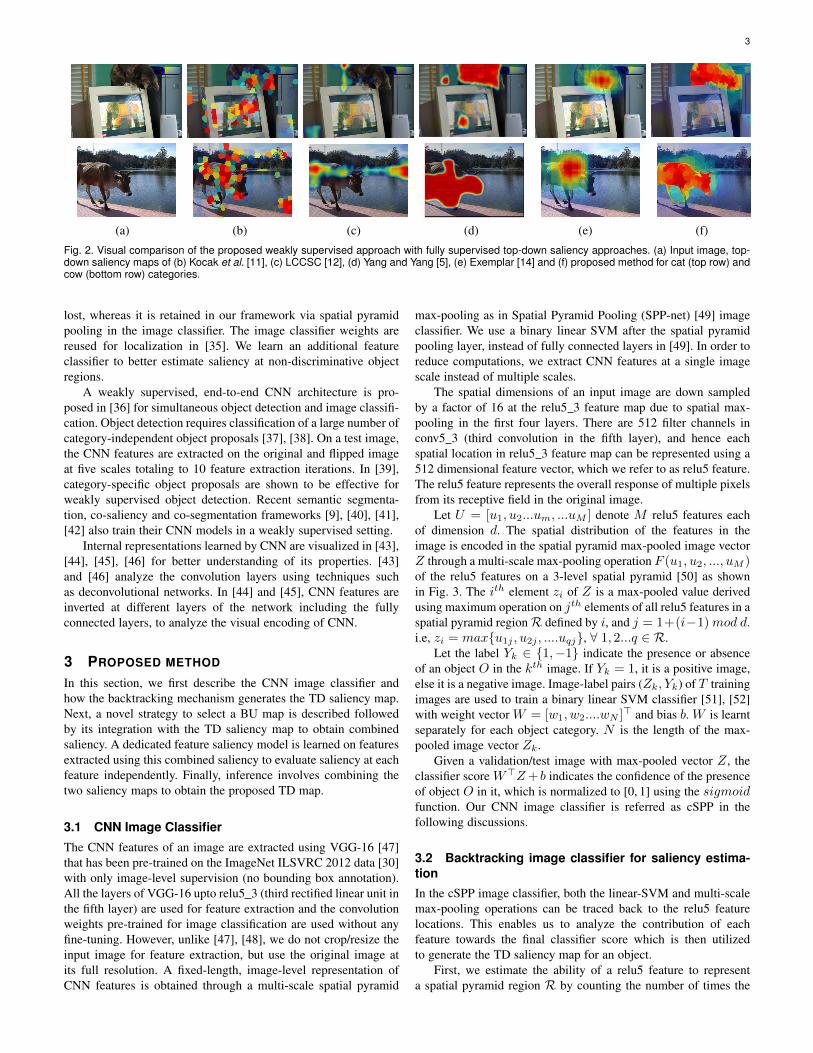
Fig. 2. Visual comparison of the proposed weakly supervised approach with fully supervised top-down saliency approaches. (a) Input image, top-down saliency maps of (b) Kocak et al. [11], (c) LCCSC [12], (d) Yang and Yang [5], (e) Exemplar [14] and (f) proposed method for cat (top row) andcow (bottom row) categories.

lost, whereas it is retained in our framework via spatial pyramidpooling in the image classifier. The image classifier weights arereused for localization in [35]. We learn an additional featureclassifier to better estimate saliency at non-discriminative objectregions.

A weakly supervised, end-to-end CNN architecture is pro-posed in [36] for simultaneous object detection and image classifi-cation. Object detection requires classification of a large number ofcategory-independent object proposals [37], [38]. On a test image,the CNN features are extracted on the original and flipped imageat five scales totaling to 10 feature extraction iterations. In [39],category-specific object proposals are shown to be effective forweakly supervised object detection. Recent semantic segmenta-tion, co-saliency and co-segmentation frameworks [9], [40], [41],[42] also train their CNN models in a weakly supervised setting.

Internal representations learned by CNN are visualized in [43],[44], [45], [46] for better understanding of its properties. [43]and [46] analyze the convolution layers using techniques suchas deconvolutional networks. In [44] and [45], CNN features areinverted at different layers of the network including the fullyconnected layers, to analyze the visual encoding of CNN.

3 PROPOSED METHOD

In this section, we first describe the CNN image classifier andhow the backtracking mechanism generates the TD saliency map.Next, a novel strategy to select a BU map is described followedby its integration with the TD saliency map to obtain combinedsaliency. A dedicated feature saliency model is learned on featuresextracted using this combined saliency to evaluate saliency at eachfeature independently. Finally, inference involves combining thetwo saliency maps to obtain the proposed TD map.

3.1 CNN Image Classifier

The CNN features of an image are extracted using VGG-16 [47]that has been pre-trained on the ImageNet ILSVRC 2012 data [30]with only image-level supervision (no bounding box annotation).All the layers of VGG-16 upto relu5 3 (third rectified linear unit inthe fifth layer) are used for feature extraction and the convolutionweights pre-trained for image classification are used without anyfine-tuning. However, unlike [47], [48], we do not crop/resize theinput image for feature extraction, but use the original image atits full resolution. A fixed-length, image-level representation ofCNN features is obtained through a multi-scale spatial pyramid

max-pooling as in Spatial Pyramid Pooling (SPP-net) [49] imageclassifier. We use a binary linear SVM after the spatial pyramidpooling layer, instead of fully connected layers in [49]. In order toreduce computations, we extract CNN features at a single imagescale instead of multiple scales.

The spatial dimensions of an input image are down sampledby a factor of 16 at the relu5 3 feature map due to spatial max-pooling in the first four layers. There are 512 filter channels inconv5 3 (third convolution in the fifth layer), and hence eachspatial location in relu5 3 feature map can be represented using a512 dimensional feature vector, which we refer to as relu5 feature.The relu5 feature represents the overall response of multiple pixelsfrom its receptive field in the original image.

Let U = [u1, u2...um, ...uM ] denote M relu5 features eachof dimension d. The spatial distribution of the features in theimage is encoded in the spatial pyramid max-pooled image vectorZ through a multi-scale max-pooling operation F (u1, u2, ..., uM )of the relu5 features on a 3-level spatial pyramid [50] as shownin Fig. 3. The ith element zi of Z is a max-pooled value derivedusing maximum operation on jth elements of all relu5 features in aspatial pyramid regionR defined by i, and j = 1+(i−1)mod d.i.e, zi = maxu1j , u2j , ....uqj, ∀ 1, 2...q ∈ R.

Let the label Yk ∈ 1,−1 indicate the presence or absenceof an object O in the kth image. If Yk = 1, it is a positive image,else it is a negative image. Image-label pairs (Zk, Yk) of T trainingimages are used to train a binary linear SVM classifier [51], [52]with weight vector W = [w1, w2....wN ]> and bias b. W is learntseparately for each object category. N is the length of the max-pooled image vector Zk.

Given a validation/test image with max-pooled vector Z , theclassifier score W>Z+ b indicates the confidence of the presenceof object O in it, which is normalized to [0, 1] using the sigmoidfunction. Our CNN image classifier is referred as cSPP in thefollowing discussions.

3.2 Backtracking image classifier for saliency estima-tionIn the cSPP image classifier, both the linear-SVM and multi-scalemax-pooling operations can be traced back to the relu5 featurelocations. This enables us to analyze the contribution of eachfeature towards the final classifier score which is then utilizedto generate the TD saliency map for an object.

First, we estimate the ability of a relu5 feature to representa spatial pyramid region R by counting the number of times the

4

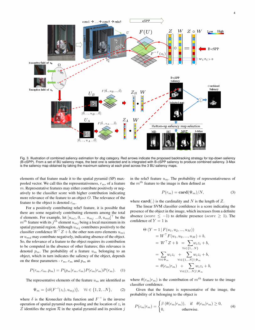
Fig. 3. Illustration of combined saliency estimation for dog category. Red arrows indicate the proposed backtracking strategy for top-down saliency(B-cSPP). From a set of BU saliency maps, the best one is selected and is integrated with B-cSPP saliency to produce combined saliency. 3-Maxis the saliency map obtained by taking the maximum saliency at each pixel across the 3 BU saliency maps.

elements of that feature made it to the spatial pyramid (SP) max-pooled vector. We call this the representativeness, rm, of a featurem. Representative features may either contribute positively or neg-atively to the classifier score with higher contribution indicatingmore relevance of the feature to an object O. The relevance of thefeature to the object is denoted cm.

For a positively contributing relu5 feature, it is possible thatthere are some negatively contributing elements among the totald elements. For example, let [um1, 0, ... umj ...0, umd]

> be themth feature with its jth element umj being a local maximum in itsspatial pyramid region. Although umj contributes positively to theclassifier confidence W>Z + b, the other non-zero elements um1

or umd may contribute negatively, indicating absence of the object.So, the relevance of a feature to the object requires its contributionto be computed in the absence of other features; this relevance isdenoted pm. The probability of a feature um belonging to anobject, which in turn indicates the saliency of the object, dependson the three parameters - rm, cm and pm as

P (rm, cm, pm) = P (pm|rm, cm)P (cm|rm)P (rm). (1)

The representative elements of the feature um are identified as

Ψm = iδ(F−1(zi), umj), ∀i ∈ 1, 2, ..N, (2)

where δ is the Kronecker delta function and F−1 is the inverseoperation of spatial pyramid max-pooling and the location of zi inZ identifies the region R in the spatial pyramid and its position j

in the relu5 feature um. The probability of representativeness ofthe mth feature to the image is then defined as

P (rm) = card(Ψm)/N, (3)

where card(.) is the cardinality and N is the length of Z.The linear SVM classifier confidence is a score indicating the

presence of the object in the image, which increases from a definiteabsence (score ≤ −1) to definite presence (score ≥ 1). Theconfidence of Y = 1 is

Θ (Y = 1 |F (u1, u2, ..., uM ))

= W>F (u1, u2, ..., uM ) + b,

= W>Z + b =∑

∀i∈1,..N

wizi + b,

=∑∀i∈Ψm

wizi +∑

∀i∈1,..N\Ψm

wizi + b,

= θ(cm|rm) +∑

∀i∈1,..N\Ψm

wizi + b,

where θ(cm|rm) is the contribution of mth feature to the imageclassifier confidence.

Given that the feature is representative of the image, theprobability of it belonging to the object is

P (cm|rm) =

β (θ(cm|rm)), if θ(cm|rm) ≥ 0,

0, otherwise.(4)

5

where β is the sigmoid function that maps the confidence scoreto [0, 1]. Using the above probabilities, we select a set Ω of allfeatures that contribute positively to the classifier confidence as

Ω = P (cm|rm)P (rm) > 0, ∀m = 1, 2, ..., M. (5)

The net contribution of a feature m ∈ Ω in the absence ofother features is

P (pm|rm, cm) = β (W>F (~0.., um, ...,~0) + b), (6)

where F (~0.., um, ...,~0) is the spatial pyramid max-pooling oper-ation performed by replacing all features except um with a zerovector ~0 of size d to form max-pooled vector Zm.

Implementation. Fig. 3 illustrates three relu5 features uA, uBand uC . The confidence of the presence of object O in an imageis indicated by the classifier score W>Z + b as mentioned inthe previous section and the element zi of Z has a correspondingweight wi. The elements from the Hadamard product W Z withwizi > 0 mark the features uA and uB that contribute positivelyto the classifier confidence through a F−1(.) operation, i.e the setΩ. The contribution of feature uA in the absence of other featuresis evaluated using max-pooling operations F (~0.., uA, ..,~0) inwhich all features except uA are replaced with ~0 forming max-pooled vector ZA. The saliency of a feature m is given by

P (rm, cm, pm) =

β (W>F (~0.., um, ..,~0) + b) if m ∈ Ω,

0 otherwise.(7)

Since this TD saliency of a feature is arrived at by backtracking thecSPP classifier, we call it B-cSPP saliency and the correspondingsaliency map as B-cSPP saliency map. The feature uA from theobject (dog) region is assigned high B-cSPP saliency while uBfrom background is assigned zero B-cSPP saliency.

3.3 Selection of bottom-up saliency mapAs mentioned in Section 1, TD saliency helps prune out spu-rious BU saliency points to obtain a more accurate focus-of-attention [5], [10]. In this section, we propose a novel strategyto select the best saliency map from a set of BU maps based onsaliency-weighted max pooling [19].

State-of-the-art BU saliency approaches [4], [7] can producea category-independent saliency map for an image within 40milliseconds. They assume image boundaries as the backgroundwhile approaches such as [8] focus on feature contrast to esti-mate saliency. These approaches do not require any training andgive reasonably good results. Since BU saliency maps are task-independent from a user’s perspective, the definition of ‘goodsaliency map’ varies based on the application. For example,consider Fig. 1, where four different objects are present. If a usersearches for a ‘person’ in the image, BU approaches [4], [7] thatassume image boundary as the background fail to produce a ‘goodsaliency map’. In such scenarios, an approach [8] that does not usesuch assumptions can produce better results. Thus, our objectiveis to develop a strategy to select a BU saliency method for aparticular image that is best suited for the task at hand.

Our cSPP image classifier (W, b) which was trained to esti-mate the presence of object O in an image is employed to select aBU saliency map suitable for the task of identifying image regionsthat belong to object O. To achieve a one-to-one correspondencebetween pixels in the BU saliency map and the relu5 features, wedownsample the saliency maps to the spatial resolution of feature

map at relu5 3 , i.e, by a factor of 16. From nρ BU saliencymaps, we need to select one for which features that belong to anobject are assigned high saliency and those that do not belong toan object are assigned low saliency. For a max-pooled vector Z ofan image, the SVM predicts a confidence score W>Z + b whichis proportional to the confidence of object presence in that image.i.e,

Θ (Y = 1 |Z)

= W>Z + b =∑

∀i∈1,..N

wizi + b,

=∑∀i∈ I+

wizi +∑∀i∈I−

wizi + b.

Θ (Y = 1 |Z) =∑∀i∈I+

wizi−∑∀i∈I−

|wi|zi + b (8)

where

I+ = i | wi > 0, ∀i ∈ 1, 2, ..N,

I− = i | wi < 0, ∀i ∈ 1, 2, ..N.

Ideally, features belonging to object O contribute positively tothe classifier confidence and hence they correspond to elementsin Z whose indices belong to I+, while the background featuresresult in I− indices. It is to be noted that zi is non-negative sinceit is derived from relu5 through max-pooling operation.

First, the mth feature um is weighted with ρtm, the BUsaliency value for that feature estimated by tth approach. i.e,um = um × ρtm. The saliency-weighted relu5 features U =[u1 , u2...um, ...uM ] are used to estimate the saliency-weightedmax-pooled vector Z and similar to Eq. (8), the modified confi-dence score B(t) = Θ (Y = 1 | Z) due to the tth BU map iscomputed as,

B(t) =∑∀i∈I+


|wi|zi + b. (9)

If higher values in the saliency map produced by algorithm t fallsexactly on the object regions, the second summation will be largelyreduced, due to weighting background indices with low saliencyvalues and hence B(t) will be high. If some of the backgroundalso garners high saliency, then B will be relatively low. In orderto reinforce the above assertion, we invert the saliency map (bysubtracting saliency values from the maximum saliency valuein the image), and recompute the saliency-weighted max-pooledvector Z and B(t) using same procedure. i.e,

B(t) =∑∀i∈I+


|wi|zi + b. (10)

If all object regions are assigned with higher saliency values inEq. (10), higher weights are assigned to the background regionsand lower weights to the salient regions, leading to a lower scoreof B(t). Combining the above two observations, an ideal saliencymap should maximize

B(t)− B(t) =∑∀i∈I+

wi(zi − zi)−∑∀i∈I−|wi| (zi − zi). (11)

In order to prevent the selection of a map that assigns highsaliency to the entire image, we impose a penalty of 1 − µt onsaliency map t with a mean saliency µt. Combining the aboveobservations, the final objective function to select a BU saliencymap is

6

B(t) = ∑∀i∈I+

wi(zi− zi)−∑∀i∈I−|wi| (zi− zi)×(1−µt). (12)

If the saliency map of tth algorithm is not aligned with the object,then the false positives will increase zi and decrease z in I−, thusincreasing the second term of Eq. (12). False negatives will reducezi and increase z reducing the first term. Hence an inaccurateBU saliency map will result in low B(t). The saliency map thatmaximizes Eq. (12) is selected.

In addition to choosing individual BU saliency maps, we alsoanalyze whether a combination of these maps has an effect onimproving TD saliency. To this end, we combine saliency mapsby picking the maximum saliency for each pixel and use Eq. (12)to select the best map from a set of saliency maps that includesthe maximum map. In this section, we have assumed that the SVMweights learnt for an object is accurate and that the object appearsonly at locations where wi are positive. Although this may not bealways true, we retain this assumption since object locations arenot available in a weakly supervised setting.

The B-cSPP saliency map and the selected bottom up saliencymap are combined through a simple multiplication as shown inFig. 3. We denote this combined saliency map as H. Following[5], [10], [11], we also characterize our category-specific saliencyinference framework as TD saliency even though there is a bottom-up component.

3.4 Feature saliency trainingImage classifiers trained on image-level representation of featureshave shown to be effective in discriminative TD saliency estima-tion [10], [15], [23]. The combined saliency map H takes non-zero values only at discriminative image regions whose featuresmake positive contribution to the image classifier confidence.The assumption is that the object appears only at grids in thespatial pyramid where wi are positive, which may not be trueacross all images. Our objective is not limited to identifyingthe discriminative image regions, but to assign higher saliencyvalues to all pixels belonging to the salient object. In order toindependently estimate the saliency value of each relu5 feature,we also learn a top-down feature saliency model that uses alinear SVM learnt on positive and negative relu5 features from thetraining images. Since feature-level annotation is not available, weuse object features extracted using the combined saliency map Hto train the model.

From positive training images of object O, relu5 features withH saliency greater than 0.5 are selected as positive features withlabel l = +1. In order to prevent training features from non-discriminative object regions of positive images with negativelabel, only those features at which both B-cSSP and BU saliencyare selected as negative features with label l = −1. Additionally,random features are selected from negative images with labell = −1. A linear SVM model with weight v and bias bv islearned. Since the relu5 features are already computed for B-cSPP,learning of linear SVM is the only additional computation requiredto train this top-down model. The saliency map obtained fromfeature saliency is denoted L.

3.5 Saliency inferenceFor inference on a test image, the combined saliencyH and featuresaliency are first integrated followed by multi-scale superpixel

averaging and finally associated with the confidence of the imageclassifier to obtain the saliency at a pixel. While the combinedsaliency is obtained as described in Section 3.3, the featuresaliency for a feature um is the probability of the feature belongingto an object computed by applying a sigmod function β to thelinear SVM score,

P (l = 1 | um, v) = β (vTum + bv). (13)

The feature saliency and combined saliency values are integratedusing a mean operation to form the saliency map, Sp = H+L

2 .

3.5.1 Multi-scale superpixel-averaging of saliency mapThe low resolution saliency map Sp is upsampled to the originalimage size using bicubic interpolation. As a consequence, saliencyvalues may not be uniform within a superpixel. Also, the saliencymap will not be edge-aware with object regions spreading to thebackground. Hence, a multi-scale superpixel-averaging strategy isemployed. The mean saliency at a superpixel (obtained by SLICsegmentation [53]) is assigned to every pixel in it. This processis repeated at multiple scales by varying the SLIC parameters.The resulting maps are averaged to produce a smooth, pixel-levelsaliency map Spix that uniformly highlights the salient object andalso produces a sharp transition at object boundaries.

3.5.2 Integrating with image classifier confidenceFor a given image, the TD saliency map Spix indicates theprobable pixels that belong to object O. Since the presence of aspecific object in a test image is not known apriori for applicationssuch as semantic segmentation and object detection, the saliencymap needs to be estimated for both positive and negative images.Hence, it is beneficial to integrate Spix with a confidence scorethat indicates the presence of object O in at least one pixel in theimage. For this, we use the same cSPP image classifiers learntearlier for each category. The SVM associated with the cSPPimage classifier gives a confidence score Φ(O) for a particularobject O as Θ (Y = 1 |Z). These scores are scaled between 0and 1 as

Φ(O) =exp(Φ(O))

max1≤j≤nc

exp(Φ(j)), (14)

where, nc is the total number of categories. Unlike soft-max thatsums to 1, we normalize the score with the maximum becausemultiple categories can simultaneously appear in an image such asin PASCAL VOC-2012 [54]. In such scenarios, softmax will endup assigning a lower value to all positive categories. However, ourobjective is to identify the relative confidence across categories,and assign 1 to the most probable category. To reduce falsedetections from less probable categories, we assume values ofΦ(O) that are less than 0.5 as less important, and replace itwith 0. This limits the number of probable object categories perimage to less than 5 categories in most images, and hence thecategory-specific saliency map Spix needs to be computed only forthese few probable object categories. We compute the classifier-weighted, category-specific score for each object O,

Scateg(O) = Spix(O) · Φ(O). (15)

3.5.3 Category-independent salient object detectionThe proposed category-specific TD saliency map Scateg inEq. (15) can be used to compute the category-independent saliency

7

value Sind, by computing the maximum saliency value at eachpixel (x,y) as

Sind(x, y) = max1≤j≤nc

Scateg(j)(x, y).

Since the bottom-up information is integrated to Scateg throughthe combined saliency map H, the Sind(x, y) gives an accurateestimate of saliency maps under free-viewing condition.

4 APPLICATIONS

TD saliency [5], [11], [14], [15] and tasks like object detection,localization and segmentation mainly differ in their granularityof representation. Object detection produces a tight rectangularbounding box around all instances of objects belonging to user-defined categories. It is necessary to identify both the locationas well as the extent of each object. The process of identifyingthe location of a particular object in an image, without markingthe extent of the object, is referred to as object localization [32].Object segmentation, also referred to as semantic object selectionproduces a binary mask with ‘1’ indicating all pixels that belong toa user-defined object category. It differs from the task of semanticsegmentation, where the objective is to classify each pixel in theimage to one of predefined classes. In this section, we detail theuse of our TD saliency framework for the above applications in aweakly supervised setting.

Semantic segmentation. The category-specific saliency mapsin the proposed framework can be easily adapted for semanticsegmentation. In the saliency map, a pixel with Scateg(O) < 0.5is less likely to belong to an object O. The pixels at which themaximum saliency across all categories is less than 0.5 is morelikely to be background. Hence, the additional map correspondingto the background category is generated as a uniform map withScateg = 0.5. We assign to each pixel the category for which itssaliency is the maximum.

Object segmentation. Conventional object segmentation ap-proaches use scribbles or rectangular boxes to indicate the objectof interest, while in our approach, only the semantic label of theobject of interest is input to the system, similar to the semanticobject selection [55]. We threshold our TD saliency map toidentify definite foreground and background regions in an image,followed by Grab-cut [56] to accurately segment out the objectof interest. Being a weakly supervised approach, framework iscomparable to co-segmentation approaches that segment out acommon object from a given set of images. We learn a modelfor the common object, which helps to achieve faster inference fora newly added test image, whereas co-segmentation approachesneed to re-segment every image in the set upon encountering anew image.

Object localization. Object localization deals with locatingobject O within a positive image. Here, only the location of theobject needs to be identified, not its extent. The peaks of oursaliency map, Spix indicates the location of object O,

Loc (O) = argmax(x, y)

SPix(O)(x, y).

Object detection. In object detection, multiple instances of thesame object category need to be identified separately. This is morechallenging than localization and especially so in a weakly super-vised setting. Conventional object detectors such as R-CNN [1],[36] need to classify thousands of category-independent objectproposals generated using selective search [37], [38]. This incurs

46.9 47

47.5

48.6

46

49.950.1

50.6

51.5

45

46

47

48

49

50

51

52

MST GP EQCUT MB 5-Max 3-Select 4-Select 5-Select 6-Select

Pix

el-le

ve

l P

recis

ion

rate

at E

ER

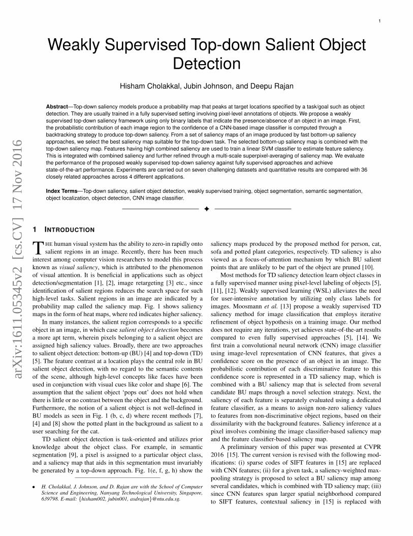
3-Select: MB+MST 4-Select: MB+MST+HC

5-Select: MB+MST+HC+GP 6-Select: B+MST+HC+GP+EQCUT

5-Max: Pixel max. of 5 maps

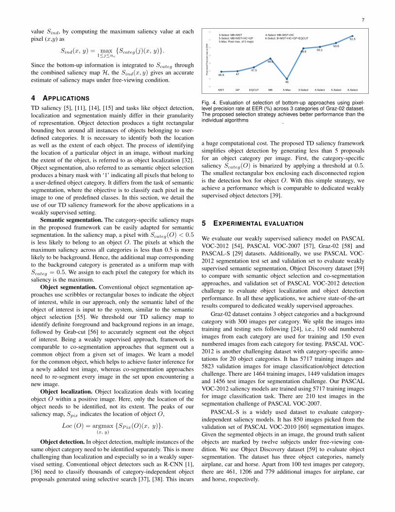
Fig. 4. Evaluation of selection of bottom-up approaches using pixel-level precision rate at EER (%) across 3 categories of Graz-02 dataset.The proposed selection strategy achieves better performance than theindividual algorithms .

a huge computational cost. The proposed TD saliency frameworksimplifies object detection by generating less than 5 proposalsfor an object category per image. First, the category-specificsaliency Scateg(O) is binarized by applying a threshold at 0.5.The smallest rectangular box enclosing each disconnected regionis the detection box for object O. With this simple strategy, weachieve a performance which is comparable to dedicated weaklysupervised object detectors [39].

5 EXPERIMENTAL EVALUATION

We evaluate our weakly supervised saliency model on PASCALVOC-2012 [54], PASCAL VOC-2007 [57], Graz-02 [58] andPASCAL-S [29] datasets. Additionally, we use PASCAL VOC-2012 segmentation test set and validation set to evaluate weaklysupervised semantic segmentation, Object Discovery dataset [59]to compare with semantic object selection and co-segmentationapproaches, and validation set of PASCAL VOC-2012 detectionchallenge to evaluate object localization and object detectionperformance. In all these applications, we achieve state-of-the-artresults compared to dedicated weakly supervised approaches.

Graz-02 dataset contains 3 object categories and a backgroundcategory with 300 images per category. We split the images intotraining and testing sets following [24], i.e., 150 odd numberedimages from each category are used for training and 150 evennumbered images from each category for testing. PASCAL VOC-2012 is another challenging dataset with category-specific anno-tations for 20 object categories. It has 5717 training images and5823 validation images for image classification/object detectionchallenge. There are 1464 training images, 1449 validation imagesand 1456 test images for segmentation challenge. Our PASCALVOC-2012 saliency models are trained using 5717 training imagesfor image classification task. There are 210 test images in thesegmentation challenge of PASCAL VOC-2007.

PASCAL-S is a widely used dataset to evaluate category-independent saliency models. It has 850 images picked from thevalidation set of PASCAL VOC-2010 [60] segmentation images.Given the segmented objects in an image, the ground truth salientobjects are marked by twelve subjects under free-viewing con-dition. We use Object Discovery dataset [59] to evaluate objectsegmentation. The dataset has three object categories, namelyairplane, car and horse. Apart from 100 test images per category,there are 461, 1206 and 779 additional images for airplane, carand horse, respectively.

8

(a) (b) (c) (d) (e)

Fig. 5. Qualitative results at individual stages of the proposed method.(a) Input image, (b) B-cSPP saliency map, (c) (b) + bottom-up saliency,(d) (c) + feature saliency, (e) (d) + superpixel averaging.

5.1 Evaluation of selection of bottom-up saliency map

Fig. 4 illustrates the performance of the proposed strategy forselection of BU saliency map on positive test images, evaluatedusing mean of pixel-level precision rates at EER across all 3 objectcategories of Graz-02 dataset. Comparing the individual perfor-mances of 5 recent unsupervised algorithms HC [8], GP [61],EQCUT [62], MST [4] and MB [7] showed that MB outperformsothers while HC has the lowest precision rate at EER. Since theY-axis of the graph in Fig. 4 is limited to a range between 45 and53, HC with mean precision rate at EER of 29.84% is not shown.Across individual categories, MB gives the best performance inbike category while EQCUT outperforms others in car and personcategories.

First, we evaluate the performance of a maximum map formedby pixel-level maximum operation across the saliency maps ofthese 5 algorithms. Since the false positives from all the mapsaccumulate due to maximum operation, the mean precision rate atEER of this maximum map drops to 46% and denoted 5-Max inFig. 4. Thus, combining BU maps without top-down informationabout the task can deteriorate the quality of the map.

Next, the proposed strategy to select the best saliency mapamong MB, MST and their maximum map is evaluated andshown as 3-Select in Fig. 4. Although MB outperforms MST inall the 3 categories, a performance boost of 1.3% is observedas a result of the selection of saliency map from MB, MST ormaximum map for those images on which it outperforms others.The same procedure is repeated for the maps of MB, MST, HCand their maximum map and denoted 4-Select. In all the threecategories, the performance of newly added HC algorithm is muchlower than other approaches (less than 35%). We still observe animprovement of 0.2% in the mean precision rate at EER of 4-Select. Our approach automatically selects the best performingMB for 50.7% of the total images, 33.5% from MST, and only8.5% from least performing HC. The remaining 7.3% are selectedfrom the maximum map.

Similarly, addition of GP improved the accuracy by 0.5% in5-Select. It is to be noted that MST, HC and GP are not thebest performing algorithms in any of the individual categories,but their addition resulted in a gradual increase in the averageaccuracy. This shows that even though these algorithms haveinferior performance in majority of the images in all 3 categories,they give better quality saliency maps for few images and theproposed selection strategy is able to accurately select thosesaliency maps.

Finally, 6-Select uses saliency maps of MB, MST, HC, GP,EQCUT, and the maximum map. In bike category, the largestnumber of maps are selected from MB (28% of bike images),which is the best performing algorithm for that category. Similarly,the largest number of car maps (23.3% ) are selected from

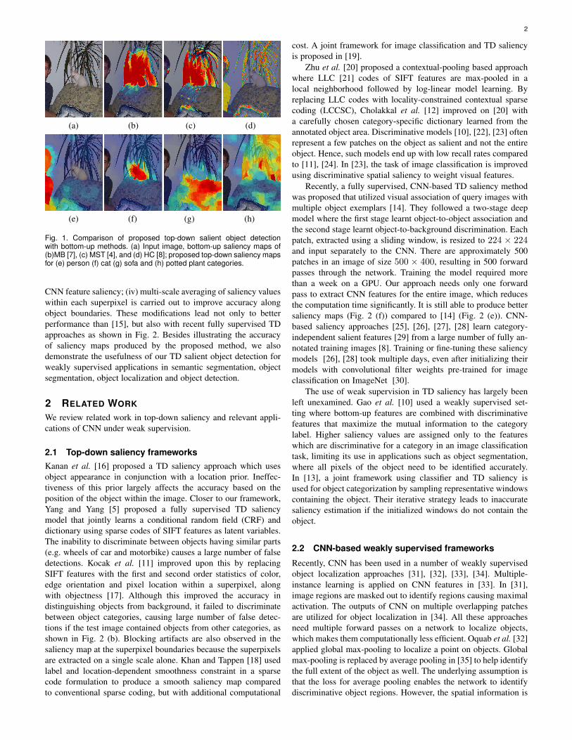
59.6

43.6

34.1

1.8

16

9.5

34.1

-8 2 12 22 32 42 52 62

+ Superpixel Averaging

+ Feature saliency

+ Bottom-up Selection

B-cSPP saliency

Improvement in accuracy due to each component

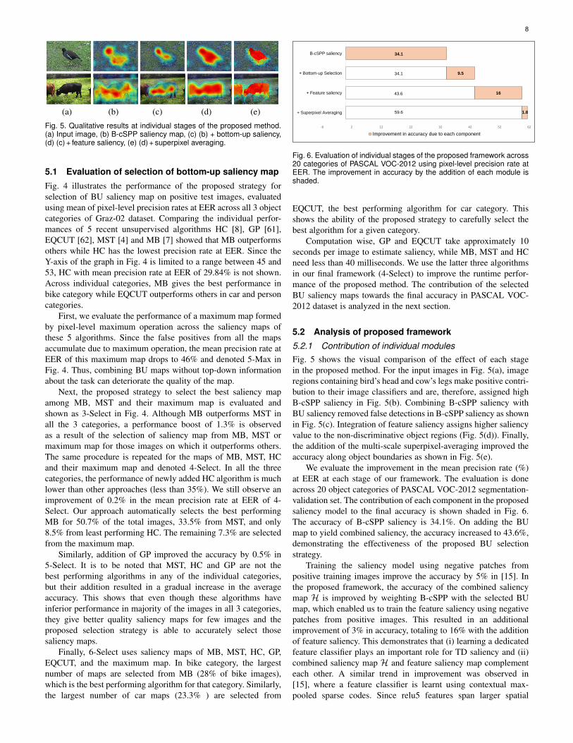
Fig. 6. Evaluation of individual stages of the proposed framework across20 categories of PASCAL VOC-2012 using pixel-level precision rate atEER. The improvement in accuracy by the addition of each module isshaded.

EQCUT, the best performing algorithm for car category. Thisshows the ability of the proposed strategy to carefully select thebest algorithm for a given category.

Computation wise, GP and EQCUT take approximately 10seconds per image to estimate saliency, while MB, MST and HCneed less than 40 milliseconds. We use the latter three algorithmsin our final framework (4-Select) to improve the runtime perfor-mance of the proposed method. The contribution of the selectedBU saliency maps towards the final accuracy in PASCAL VOC-2012 dataset is analyzed in the next section.

5.2 Analysis of proposed framework

5.2.1 Contribution of individual modulesFig. 5 shows the visual comparison of the effect of each stagein the proposed method. For the input images in Fig. 5(a), imageregions containing bird’s head and cow’s legs make positive contri-bution to their image classifiers and are, therefore, assigned highB-cSPP saliency in Fig. 5(b). Combining B-cSPP saliency withBU saliency removed false detections in B-cSPP saliency as shownin Fig. 5(c). Integration of feature saliency assigns higher saliencyvalue to the non-discriminative object regions (Fig. 5(d)). Finally,the addition of the multi-scale superpixel-averaging improved theaccuracy along object boundaries as shown in Fig. 5(e).

We evaluate the improvement in the mean precision rate (%)at EER at each stage of our framework. The evaluation is doneacross 20 object categories of PASCAL VOC-2012 segmentation-validation set. The contribution of each component in the proposedsaliency model to the final accuracy is shown shaded in Fig. 6.The accuracy of B-cSPP saliency is 34.1%. On adding the BUmap to yield combined saliency, the accuracy increased to 43.6%,demonstrating the effectiveness of the proposed BU selectionstrategy.

Training the saliency model using negative patches frompositive training images improve the accuracy by 5% in [15]. Inthe proposed framework, the accuracy of the combined saliencymap H is improved by weighting B-cSPP with the selected BUmap, which enabled us to train the feature saliency using negativepatches from positive images. This resulted in an additionalimprovement of 3% in accuracy, totaling to 16% with the additionof feature saliency. This demonstrates that (i) learning a dedicatedfeature classifier plays an important role for TD saliency and (ii)combined saliency map H and feature saliency map complementeach other. A similar trend in improvement was observed in[15], where a feature classifier is learnt using contextual max-pooled sparse codes. Since relu5 features span larger spatial

9

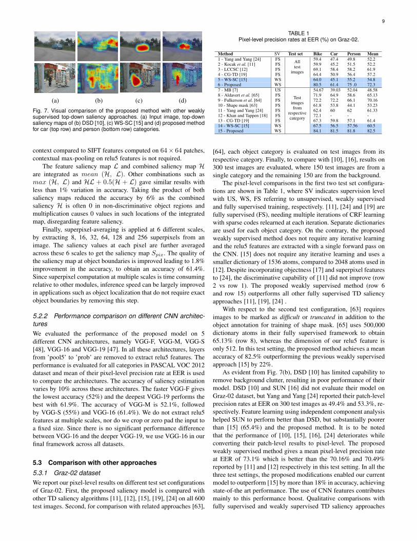
(a) (b) (c) (d)

Fig. 7. Visual comparison of the proposed method with other weaklysupervised top-down saliency approaches. (a) Input image, top-downsaliency maps of (b) DSD [10], (c) WS-SC [15] and (d) proposed methodfor car (top row) and person (bottom row) categories.

context compared to SIFT features computed on 64× 64 patches,contextual max-pooling on relu5 features is not required.

The feature saliency map L and combined saliency map Hare integrated as mean (H, L). Other combinations such asmax (H, L) and HL + 0.5(H + L) gave similar results withless than 1% variation in accuracy. Taking the product of bothsaliency maps reduced the accuracy by 6% as the combinedsaliency H is often 0 in non-discriminative object regions andmultiplication causes 0 values in such locations of the integratedmap, disregarding feature saliency.

Finally, superpixel-averaging is applied at 6 different scales,by extracting 8, 16, 32, 64, 128 and 256 superpixels from animage. The saliency values at each pixel are further averagedacross these 6 scales to get the saliency map Spix. The quality ofthe saliency map at object boundaries is improved leading to 1.8%improvement in the accuracy, to obtain an accuracy of 61.4%.Since superpixel computation at multiple scales is time consumingrelative to other modules, inference speed can be largely improvedin applications such as object localization that do not require exactobject boundaries by removing this step.

5.2.2 Performance comparison on different CNN architec-turesWe evaluated the performance of the proposed model on 5different CNN architectures, namely VGG-F, VGG-M, VGG-S[48], VGG-16 and VGG-19 [47]. In all these architectures, layersfrom ’pool5’ to ’prob’ are removed to extract relu5 features. Theperformance is evaluated for all categories in PASCAL VOC 2012dataset and mean of their pixel-level precision rate at EER is usedto compare the architectures. The accuracy of saliency estimationvaries by 10% across these architectures. The faster VGG-F givesthe lowest accuracy (52%) and the deepest VGG-19 performs thebest with 61.9%. The accuracy of VGG-M is 52.1%, followedby VGG-S (55%) and VGG-16 (61.4%). We do not extract relu5features at multiple scales, nor do we crop or zero pad the input toa fixed size. Since there is no significant performance differencebetween VGG-16 and the deeper VGG-19, we use VGG-16 in ourfinal framework across all datasets.

5.3 Comparison with other approaches

5.3.1 Graz-02 datasetWe report our pixel-level results on different test set configurationsof Graz-02. First, the proposed saliency model is compared withother TD saliency algorithms [11], [12], [15], [19], [24] on all 600test images. Second, for comparison with related approaches [63],

TABLE 1Pixel-level precision rates at EER (%) on Graz-02.

Method SV Test set Bike Car Person Mean1 - Yang and Yang [24] FS 59.4 47.4 49.8 52.22 - Kocak et al. [11] FS 59.9 45.2 51.5 52.23 - LCCSC [12] FS 69.1 58.4 58.2 61.94 - CG-TD [19] FS 64.4 50.9 56.4 57.25 - WS-SC [15] WS 64.0 45.1 55.2 54.86 - Proposed WS

Alltest

images

80.5 61.4 75 .0 72.37 - MB [7] US 54.67 39.03 52.04 48.588 - Aldavert et al. [65] FS 71.9 64.9 58.6 65.139 - Fulkerson et al. [64] FS 72.2 72.2 66.1 70.1610 - Shape mask [63] FS 61.8 53.8 44.1 53.2311 - Yang and Yang [24] FS 62.4 60 62 61.3312 - Khan and Tappen [18] FS 72.1 - - -13 - CG-TD [19] FS 67.3 59.8 57.1 61.414 - WS-SC [15] WS 67.5 56.5 57.56 60.515 - Proposed WS

Testimagesfrom

respectivecategory

84.1 81.5 81.8 82.5

[64], each object category is evaluated on test images from itsrespective category. Finally, to compare with [10], [16], results on300 test images are evaluated, where 150 test images are from asingle category and the remaining 150 are from the background.

The pixel-level comparisons in the first two test set configura-tions are shown in Table 1, where SV indicates supervision levelwith US, WS, FS referring to unsupervised, weakly supervisedand fully supervised training, respectively. [11], [24] and [19] arefully supervised (FS), needing multiple iterations of CRF learningwith sparse codes relearned at each iteration. Separate dictionariesare used for each object category. On the contrary, the proposedweakly supervised method does not require any iterative learningand the relu5 features are extracted with a single forward pass onthe CNN. [15] does not require any iterative learning and uses asmaller dictionary of 1536 atoms, compared to 2048 atoms used in[12]. Despite incorporating objectness [17] and superpixel featuresto [24], the discriminative capability of [11] did not improve (row2 vs row 1). The proposed weakly supervised method (row 6and row 15) outperforms all other fully supervised TD saliencyapproaches [11], [19], [24] .

With respect to the second test configuration, [63] requiresimages to be marked as difficult or truncated in addition to theobject annotation for training of shape mask. [65] uses 500,000dictionary atoms in their fully supervised framework to obtain65.13% (row 8), whereas the dimension of our relu5 feature isonly 512. In this test setting, the proposed method achieves a meanaccuracy of 82.5% outperforming the previous weakly supervisedapproach [15] by 22%.

As evident from Fig. 7(b), DSD [10] has limited capability toremove background clutter, resulting in poor performance of theirmodel. DSD [10] and SUN [16] did not evaluate their model onGraz-02 dataset, but Yang and Yang [24] reported their patch-levelprecision rates at EER on 300 test images as 49.4% and 53.3%, re-spectively. Feature learning using independent component analysishelped SUN to perform better than DSD, but substantially poorerthan [15] (65.4%) and the proposed method. It is to be notedthat the performance of [10], [15], [16], [24] deteriorates whileconverting their patch-level results to pixel-level. The proposedweakly supervised method gives a mean pixel-level precision rateat EER of 73.1% which is better than the 70.16% and 70.49%reported by [11] and [12] respectively in this test setting. In all thethree test settings, the proposed modifications enabled our currentmodel to outperform [15] by more than 18% in accuracy, achievingstate-of-the art performance. The use of CNN features contributesmainly to this performance boost. Qualitative comparisons withfully supervised and weakly supervised TD saliency approaches

10

TABLE 2Pixel-level precision rates at EER on validation set of PASCAL VOC-2012 segmentation dataset.The proposed weakly supervised approach

outperforms all fully supervised approaches including [14], which is based on CNN, in 14 out of 20 classes and in mean accuracy.

Method SV plane bike bird boat botl bus car cat chair cow table dog horse moto pers plant sheep sofa train tv MeanYang [24] FS 14.7 28.1 9.8 6.1 2.2 24.1 30.2 17.3 6.2 7.6 10.3 11.5 12.5 24.1 36.7 2.2 20.4 12.3 26.1 10.2 15.6Kocak [11] FS 46.5 45.0 33.1 60.2 25.8 48.4 31.4 64.4 19.8 32.2 44.7 30.1 41.8 72.1 33.0 40.5 38.6 12.2 64.6 23.6 40.4Exemplar [14] FS 55.9 37.9 45.6 43.8 47.3 83.6 57.8 69.4 22.7 68.5 37.1 72.8 63.7 69.0 57.5 43.9 66.6 38.3 75.1 56.7 56.2Oquab [32] WS 48.9 42.9 37.9 47.1 31.4 68.4 39.9 66.2 27.2 54.0 38.3 48.5 56.5 70.1 43.2 42.6 52.2 34.8 68.1 43.4 48.1Proposed WS 71.2 22.3 74.9 39.9 52.5 82.7 58.9 83.4 27.1 81.1 49.3 82.4 77.9 74.2 69.8 31.9 81.4 49.8 63.2 53.3 61.4

TABLE 3Precision rates at EER(%) on PASCAL VOC-2007.

Method Yang andYang [24] LCCSC [12] CG-TD [19] WS-SC [15] Proposed

Supervision FS FS FS WS WSMean of

20 classes 16.7 23.4 23.81 18.6 42.1

are shown in Fig. 2 and Fig. 7, respectively.

5.3.2 PASCAL VOC-2012 segmentation dataset

In Table 2, we compare a recent CNN-based fully supervisedTD saliency [14] with our method by evaluating on PASCALVOC-2012 segmentation-validation set consisting of 1449 images.Similar to [14], each object category is evaluated only on positiveimages of that category. We did not fine-tune the convolutionlayers for this dataset, which took nearly 8 days on a GPU in [14].Moreover, we only need a single CNN forward pass to extractfeatures, while [14] requires 500 forward passes for an image.The presence of multiple, visually similar object classes in a singleimage is challenging for a weakly supervised approach. Inspite ofthis, we outperform the state-of-the art fully supervised approach[14] and the CNN-based weakly supervised object localizationapproach [32] in mean accuracy by 5% and 13%, respectively.We outperform [32] in 15 out of the 20 categories. The top-downselection of BU approach along with feature saliency plays animportant role in this improved performance, especially in classeslike aeroplane and sheep.

5.3.3 PASCAL VOC-2007 segmentation dataset

Following [11], [12] and [24], the saliency models are evaluatedon 210 segmentation test images. We used the models trainedon PASCAL VOC-2012 training set in this experiment. Separatesparse codes of size 512 are computed for each category in [11],[24] and [19]. [15] uses sparse coding on a common dictionaryof 1536 atoms for all object classes. Similarly, a common featurecode of 20 × 512 = 10240 elements is used in [12]. In ourmethod, we compute 512 dimensional relu5 features which arecommon for all object categories.

Table 3 compares the pixel-level performance of the proposedWS method and patch-level results of FS top-down saliencyapproaches [12], [24] (these approaches did not report their pixel-level results on this dataset). We outperform [24], [19] and [12] inalmost all categories and in mean precision rate at EER across 20classes. A performance drop of 5 to 10% is reported by [66] whileconverting patch-level results of [24] to pixel-level, which furtherincreases the performance gain of the proposed approach. Khanand Tappen [18] report pixel-level precision rates at EER onlyfor cow category (8.5%) which is much lower than the proposedweakly supervised approach (52.3%).

58

61.1 61.6

76

6869

66.9 67.5

56

58

60

62

64

66

68

70

72

74

76

BL MST MB DHSNet MCDL MDF LEGS Proposed

Unsupervised

Fully Supervised

Weakly Supervised

F-m

easu

re s

core

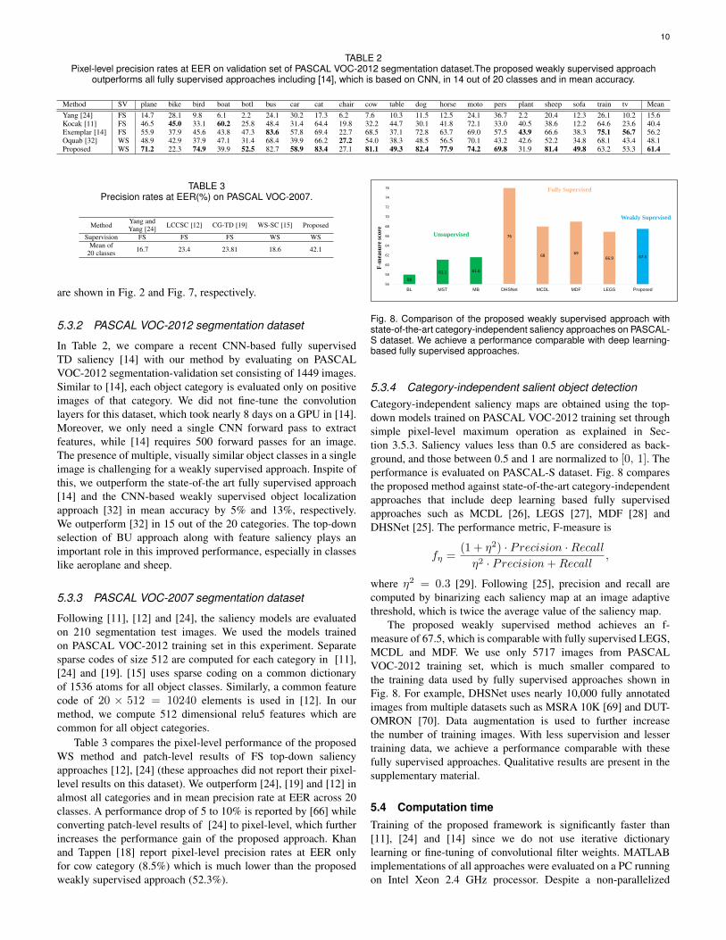
Fig. 8. Comparison of the proposed weakly supervised approach withstate-of-the-art category-independent saliency approaches on PASCAL-S dataset. We achieve a performance comparable with deep learning-based fully supervised approaches.

5.3.4 Category-independent salient object detectionCategory-independent saliency maps are obtained using the top-down models trained on PASCAL VOC-2012 training set throughsimple pixel-level maximum operation as explained in Sec-tion 3.5.3. Saliency values less than 0.5 are considered as back-ground, and those between 0.5 and 1 are normalized to [0, 1]. Theperformance is evaluated on PASCAL-S dataset. Fig. 8 comparesthe proposed method against state-of-the-art category-independentapproaches that include deep learning based fully supervisedapproaches such as MCDL [26], LEGS [27], MDF [28] andDHSNet [25]. The performance metric, F-measure is

fη =(1 + η2) · Precision ·Recallη2 · Precision+Recall

,

where η2 = 0.3 [29]. Following [25], precision and recall arecomputed by binarizing each saliency map at an image adaptivethreshold, which is twice the average value of the saliency map.

The proposed weakly supervised method achieves an f-measure of 67.5, which is comparable with fully supervised LEGS,MCDL and MDF. We use only 5717 images from PASCALVOC-2012 training set, which is much smaller compared tothe training data used by fully supervised approaches shown inFig. 8. For example, DHSNet uses nearly 10,000 fully annotatedimages from multiple datasets such as MSRA 10K [69] and DUT-OMRON [70]. Data augmentation is used to further increasethe number of training images. With less supervision and lessertraining data, we achieve a performance comparable with thesefully supervised approaches. Qualitative results are present in thesupplementary material.

5.4 Computation timeTraining of the proposed framework is significantly faster than[11], [24] and [14] since we do not use iterative dictionarylearning or fine-tuning of convolutional filter weights. MATLABimplementations of all approaches were evaluated on a PC runningon Intel Xeon 2.4 GHz processor. Despite a non-parallelized

11

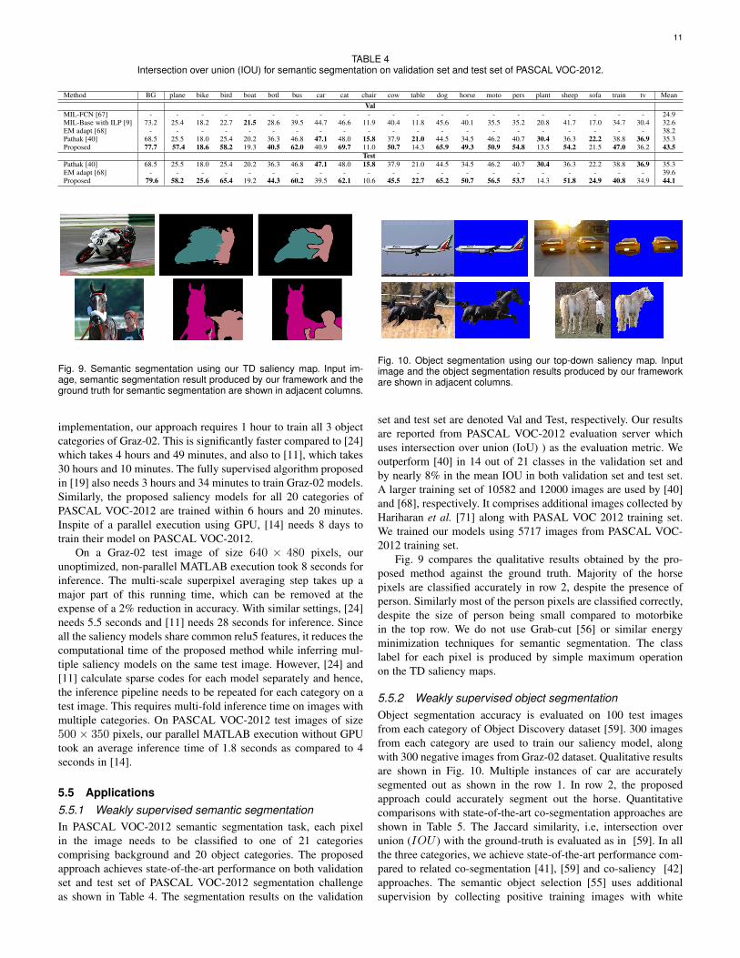
TABLE 4Intersection over union (IOU) for semantic segmentation on validation set and test set of PASCAL VOC-2012.

Method BG plane bike bird boat botl bus car cat chair cow table dog horse moto pers plant sheep sofa train tv MeanVal

MIL-FCN [67] - - - - - - - - - - - - - - - - - - - - - 24.9MIL-Base with ILP [9] 73.2 25.4 18.2 22.7 21.5 28.6 39.5 44.7 46.6 11.9 40.4 11.8 45.6 40.1 35.5 35.2 20.8 41.7 17.0 34.7 30.4 32.6EM adapt [68] - - - - - - - - - - - - - - - - - - - - - 38.2Pathak [40] 68.5 25.5 18.0 25.4 20.2 36.3 46.8 47.1 48.0 15.8 37.9 21.0 44.5 34.5 46.2 40.7 30.4 36.3 22.2 38.8 36.9 35.3Proposed 77.7 57.4 18.6 58.2 19.3 40.5 62.0 40.9 69.7 11.0 50.7 14.3 65.9 49.3 50.9 54.8 13.5 54.2 21.5 47.0 36.2 43.5

TestPathak [40] 68.5 25.5 18.0 25.4 20.2 36.3 46.8 47.1 48.0 15.8 37.9 21.0 44.5 34.5 46.2 40.7 30.4 36.3 22.2 38.8 36.9 35.3EM adapt [68] - - - - - - - - - - - - - - - - - - - - - 39.6Proposed 79.6 58.2 25.6 65.4 19.2 44.3 60.2 39.5 62.1 10.6 45.5 22.7 65.2 50.7 56.5 53.7 14.3 51.8 24.9 40.8 34.9 44.1

Fig. 9. Semantic segmentation using our TD saliency map. Input im-age, semantic segmentation result produced by our framework and theground truth for semantic segmentation are shown in adjacent columns.

implementation, our approach requires 1 hour to train all 3 objectcategories of Graz-02. This is significantly faster compared to [24]which takes 4 hours and 49 minutes, and also to [11], which takes30 hours and 10 minutes. The fully supervised algorithm proposedin [19] also needs 3 hours and 34 minutes to train Graz-02 models.Similarly, the proposed saliency models for all 20 categories ofPASCAL VOC-2012 are trained within 6 hours and 20 minutes.Inspite of a parallel execution using GPU, [14] needs 8 days totrain their model on PASCAL VOC-2012.

On a Graz-02 test image of size 640 × 480 pixels, ourunoptimized, non-parallel MATLAB execution took 8 seconds forinference. The multi-scale superpixel averaging step takes up amajor part of this running time, which can be removed at theexpense of a 2% reduction in accuracy. With similar settings, [24]needs 5.5 seconds and [11] needs 28 seconds for inference. Sinceall the saliency models share common relu5 features, it reduces thecomputational time of the proposed method while inferring mul-tiple saliency models on the same test image. However, [24] and[11] calculate sparse codes for each model separately and hence,the inference pipeline needs to be repeated for each category on atest image. This requires multi-fold inference time on images withmultiple categories. On PASCAL VOC-2012 test images of size500 × 350 pixels, our parallel MATLAB execution without GPUtook an average inference time of 1.8 seconds as compared to 4seconds in [14].

5.5 Applications5.5.1 Weakly supervised semantic segmentationIn PASCAL VOC-2012 semantic segmentation task, each pixelin the image needs to be classified to one of 21 categoriescomprising background and 20 object categories. The proposedapproach achieves state-of-the-art performance on both validationset and test set of PASCAL VOC-2012 segmentation challengeas shown in Table 4. The segmentation results on the validation

Fig. 10. Object segmentation using our top-down saliency map. Inputimage and the object segmentation results produced by our frameworkare shown in adjacent columns.

set and test set are denoted Val and Test, respectively. Our resultsare reported from PASCAL VOC-2012 evaluation server whichuses intersection over union (IoU) ) as the evaluation metric. Weoutperform [40] in 14 out of 21 classes in the validation set andby nearly 8% in the mean IOU in both validation set and test set.A larger training set of 10582 and 12000 images are used by [40]and [68], respectively. It comprises additional images collected byHariharan et al. [71] along with PASAL VOC 2012 training set.We trained our models using 5717 images from PASCAL VOC-2012 training set.

Fig. 9 compares the qualitative results obtained by the pro-posed method against the ground truth. Majority of the horsepixels are classified accurately in row 2, despite the presence ofperson. Similarly most of the person pixels are classified correctly,despite the size of person being small compared to motorbikein the top row. We do not use Grab-cut [56] or similar energyminimization techniques for semantic segmentation. The classlabel for each pixel is produced by simple maximum operationon the TD saliency maps.

5.5.2 Weakly supervised object segmentationObject segmentation accuracy is evaluated on 100 test imagesfrom each category of Object Discovery dataset [59]. 300 imagesfrom each category are used to train our saliency model, alongwith 300 negative images from Graz-02 dataset. Qualitative resultsare shown in Fig. 10. Multiple instances of car are accuratelysegmented out as shown in the row 1. In row 2, the proposedapproach could accurately segment out the horse. Quantitativecomparisons with state-of-the-art co-segmentation approaches areshown in Table 5. The Jaccard similarity, i.e, intersection overunion (IOU ) with the ground-truth is evaluated as in [59]. In allthe three categories, we achieve state-of-the-art performance com-pared to related co-segmentation [41], [59] and co-saliency [42]approaches. The semantic object selection [55] uses additionalsupervision by collecting positive training images with white

12

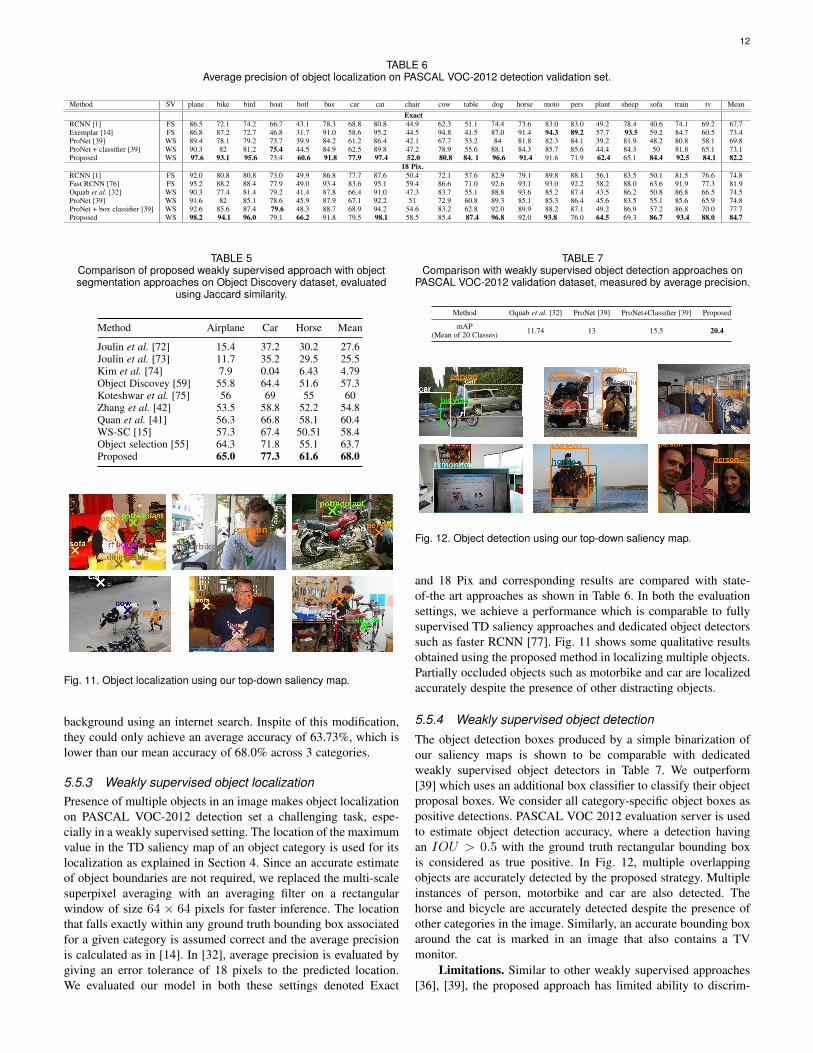
TABLE 6Average precision of object localization on PASCAL VOC-2012 detection validation set.

Method SV plane bike bird boat botl bus car cat chair cow table dog horse moto pers plant sheep sofa train tv MeanExact

RCNN [1] FS 86.5 72.1 74.2 66.7 43.1 78.3 68.8 80.8 44.9 62.3 51.1 74.4 73.6 83.0 83.0 49.2 78.4 40.6 74.1 69.2 67.7Exemplar [14] FS 86.8 87.2 72.7 46.8 31.7 91.0 58.6 95.2 44.5 94.8 41.5 87.0 91.4 94.3 89.2 57.7 93.5 59.2 84.7 60.5 73.4ProNet [39] WS 89.4 78.1 79.2 73.7 39.9 84.2 61.2 86.4 42.1 67.7 53.2 84 81.8 82.3 84.1 39.2 81.9 48.2 80.8 58.1 69.8ProNet + classifier [39] WS 90.3 82 81.2 75.4 44.5 84.9 62.5 89.8 47.2 78.9 55.6 88.1 84.3 85.7 85.6 44.4 84.3 50 81.8 65.1 73.1Proposed WS 97.6 93.1 95.6 73.4 60.6 91.8 77.9 97.4 52.0 80.8 84. 1 96.6 91.4 91.6 71.9 62.4 65.1 84.4 92.5 84.1 82.2

18 Pix.RCNN [1] FS 92.0 80.8 80.8 73.0 49.9 86.8 77.7 87.6 50.4 72.1 57.6 82.9 79.1 89.8 88.1 56.1 83.5 50.1 81.5 76.6 74.8Fast RCNN [76] FS 95.2 88.2 88.4 77.9 49.0 93.4 83.6 95.1 59.4 86.6 71.0 92.6 93.1 93.0 92.2 58.2 88.0 63.6 91.9 77.3 81.9Oquab et al. [32] WS 90.3 77.4 81.4 79.2 41.4 87.8 66.4 91.0 47.3 83.7 55.1 88.8 93.6 85.2 87.4 43.5 86.2 50.8 86.8 66.5 74.5ProNet [39] WS 91.6 82 85.1 78.6 45.9 87.9 67.1 92.2 51 72.9 60.8 89.3 85.1 85.3 86.4 45.6 83.5 55.1 85.6 65.9 74.8ProNet + box classifier [39] WS 92.6 85.6 87.4 79.6 48.3 88.7 68.9 94.2 54.6 83.2 62.8 92.0 89.9 88.2 87.1 49.2 86.9 57.2 86.8 70.0 77.7Proposed WS 98.2 94.1 96.0 79.1 66.2 91.8 79.5 98.1 58.5 85.4 87.4 96.8 92.0 93.8 76.0 64.5 69.3 86.7 93.4 88.0 84.7

TABLE 5Comparison of proposed weakly supervised approach with objectsegmentation approaches on Object Discovery dataset, evaluated

using Jaccard similarity.

Method Airplane Car Horse Mean

Joulin et al. [72] 15.4 37.2 30.2 27.6Joulin et al. [73] 11.7 35.2 29.5 25.5Kim et al. [74] 7.9 0.04 6.43 4.79Object Discovey [59] 55.8 64.4 51.6 57.3Koteshwar et al. [75] 56 69 55 60Zhang et al. [42] 53.5 58.8 52.2 54.8Quan et al. [41] 56.3 66.8 58.1 60.4WS-SC [15] 57.3 67.4 50.51 58.4Object selection [55] 64.3 71.8 55.1 63.7Proposed 65.0 77.3 61.6 68.0

Fig. 11. Object localization using our top-down saliency map.

background using an internet search. Inspite of this modification,they could only achieve an average accuracy of 63.73%, which islower than our mean accuracy of 68.0% across 3 categories.

5.5.3 Weakly supervised object localizationPresence of multiple objects in an image makes object localizationon PASCAL VOC-2012 detection set a challenging task, espe-cially in a weakly supervised setting. The location of the maximumvalue in the TD saliency map of an object category is used for itslocalization as explained in Section 4. Since an accurate estimateof object boundaries are not required, we replaced the multi-scalesuperpixel averaging with an averaging filter on a rectangularwindow of size 64 × 64 pixels for faster inference. The locationthat falls exactly within any ground truth bounding box associatedfor a given category is assumed correct and the average precisionis calculated as in [14]. In [32], average precision is evaluated bygiving an error tolerance of 18 pixels to the predicted location.We evaluated our model in both these settings denoted Exact

TABLE 7Comparison with weakly supervised object detection approaches on

PASCAL VOC-2012 validation dataset, measured by average precision.

Method Oquab et al. [32] ProNet [39] ProNet+Classifier [39] Proposed

mAP(Mean of 20 Classes) 11.74 13 15.5 20.4

Fig. 12. Object detection using our top-down saliency map.

and 18 Pix and corresponding results are compared with state-of-the art approaches as shown in Table 6. In both the evaluationsettings, we achieve a performance which is comparable to fullysupervised TD saliency approaches and dedicated object detectorssuch as faster RCNN [77]. Fig. 11 shows some qualitative resultsobtained using the proposed method in localizing multiple objects.Partially occluded objects such as motorbike and car are localizedaccurately despite the presence of other distracting objects.

5.5.4 Weakly supervised object detection

The object detection boxes produced by a simple binarization ofour saliency maps is shown to be comparable with dedicatedweakly supervised object detectors in Table 7. We outperform[39] which uses an additional box classifier to classify their objectproposal boxes. We consider all category-specific object boxes aspositive detections. PASCAL VOC 2012 evaluation server is usedto estimate object detection accuracy, where a detection havingan IOU > 0.5 with the ground truth rectangular bounding boxis considered as true positive. In Fig. 12, multiple overlappingobjects are accurately detected by the proposed strategy. Multipleinstances of person, motorbike and car are also detected. Thehorse and bicycle are accurately detected despite the presence ofother categories in the image. Similarly, an accurate bounding boxaround the cat is marked in an image that also contains a TVmonitor.

Limitations. Similar to other weakly supervised approaches[36], [39], the proposed approach has limited ability to discrim-

13

inate among multiple instances of an object which are spatiallyadjacent. This causes low performance for object detection, com-pared to state-of-the-art fully supervised object detectors [78].Examples are provided in the supplementary material.

6 CONCLUSION

In this paper, a CNN feature-based weakly supervised salientobject detection approach is proposed. A novel strategy to selecta BU saliency map that suits a top-down task is proposed.Contribution of relu5 features at different spatial locations areestimated to compute a novel B-cSPP saliency. The top-downB-cSPP saliency is integrated with the BU saliency map andproduces a combined saliency which is further integrated with fea-ture saliency. The proposed weakly supervised top-down saliencymodel achieves state-of-the-art performance in top-down salientobject detection by outperforming even fully supervised CNN-based approaches. Moreover, the top-down saliency maps ofdifferent object categories are combined to produce a category-independent saliency map that can estimate salient objects underfree-viewing condition. Finally, through quantitative comparisons,we demonstrated the usefulness of proposed saliency map for fourdifferent applications. We plan to extend our framework to videosfor weakly supervised salient object detection.

REFERENCES

[1] R. Girshick, J. Donahue, T. Darrell, and J. Malik, “Rich feature hierar-chies for accurate object detection and semantic segmentation,” in Proc.IEEE Conf. Comput. Vis. Pattern Recognit., 2014, pp. 580–587.

[2] Y. Jia and M. Han, “Category-independent object-level saliency detec-tion,” in Proc. IEEE Int. Conf. Comput. Vis., 2013.

[3] D. Vaquero, M. Turk, K. Pulli, M. Tico, and N. Gelfand, “A survey of im-age retargeting techniques,” in SPIE Optical Engineering + Applications,2010, pp. 779–814.

[4] W.-C. Tu, S. He, Q. Yang, and S.-Y. Chien, “Real-time salient objectdetection with a minimum spanning tree,” in Proc. IEEE Conf. Comput.Vis. Pattern Recognit., June 2016.

[5] J. Yang and M.-H. Yang, “Top-down visual saliency via joint crf anddictionary learning,” IEEE Trans. Pattern Anal. Mach. Intell., 2016.

[6] T. Liu, Z. Yuan, J. Sun, J. Wang, N. Zheng, X. Tang, and H.-Y. Shum,“Learning to detect a salient object,” IEEE Trans. Pattern Anal. Mach.Intell., vol. 33, no. 2, pp. 353–367, 2011.

[7] J. Zhang, S. Sclaroff, Z. Lin, X. Shen, B. Price, and R. Mech, “Minimumbarrier salient object detection at 80 fps,” in Proc. IEEE Int. Conf.Comput. Vis., 2015.

[8] M. M. Cheng, N. J. Mitra, X. Huang, P. H. S. Torr, and S. M. Hu, “Globalcontrast based salient region detection,” IEEE Trans. Pattern Anal. Mach.Intell., vol. 37, no. 3, pp. 569–582, March 2015.

[9] P. O. Pinheiro and R. Collobert, “Weakly supervised semantic segmen-tation with convolutional networks,” in Proc. IEEE Conf. Comput. Vis.Pattern Recognit., vol. 2, no. 5, 2015, p. 6.

[10] D. Gao, S. Han, and N. Vasconcelos, “Discriminant saliency, the detec-tion of suspicious coincidences, and applications to visual recognition,”IEEE Trans. Pattern Anal. Mach. Intell., vol. 31, no. 6, pp. 989–1005,2009.

[11] A. Kocak, K. Cizmeciler, A. Erdem, and E. Erdem, “Top down saliencyestimation via superpixel-based discriminative dictionaries,” in Proc.British Mach. Vis. Conf., 2014.

[12] H. Cholakkal, D. Rajan, and J. Johnson, “Top-down saliency withlocality-constrained contextual sparse coding,” in Proc. British Mach.Vis. Conf., 2015.

[13] F. Moosmann, E. Nowak, and F. Jurie, “Randomized clustering forestsfor image classification,” IEEE Trans. Pattern Anal. Mach. Intell., vol. 30,no. 9, pp. 1632–1646, Sept 2008.

[14] S. He, R. W. Lau, and Q. Yang, “Exemplar-driven top-down saliencydetection via deep association,” in Proc. IEEE Conf. Comput. Vis. PatternRecognit., 2016.

[15] H. Cholakkal, J. Johnson, and D. Rajan, “Backtracking scspm imageclassifier for weakly supervised top-down saliency,” in Proc. IEEE Conf.Comput. Vis. Pattern Recognit., 2016.

[16] C. Kanan, M. H. Tong, L. Zhang, and G. W. Cottrell, “Sun: Top-downsaliency using natural statistics,” Vis. cogn., vol. 17, no. 6-7, pp. 979–1003, 2009.

[17] B. Alexe, T. Deselaers, and V. Ferrari, “What is an object?” in Proc.IEEE Conf. Comput. Vis. Pattern Recognit., 2010.

[18] N. Khan and M. F. Tappen, “Discriminative dictionary learning withspatial priors.” in Proc. Int. Conf. Image Proc., 2013.

[19] H. Cholakkal, J. Johnson, and D. Rajan, “A classifier-guided approachfor top-down salient object detection,” Signal Process. Image Commun.,vol. 45, pp. 24–40, 2016.

[20] J. Zhu, Y. Qiu, R. Zhang, J. Huang, and W. Zhang, “Top-down saliencydetection via contextual pooling,” J. Signal Process. Syst., vol. 74, no. 1,pp. 33–46, 2014.

[21] J. Wang, J. Yang, K. Yu, F. Lv, T. Huang, and Y. Gong, “Locality-constrained linear coding for image classification,” in Proc. IEEE Conf.Comput. Vis. Pattern Recognit., 2010.

[22] B. Yao, A. Khosla, and L. Fei-Fei, “Combining randomization anddiscrimination for fine-grained image categorization,” in Proc. IEEEConf. Comput. Vis. Pattern Recognit., 2011.

[23] G. Sharma, F. Jurie, and C. Schmid, “Discriminative spatial saliencyfor image classification,” in Proc. IEEE Conf. Comput. Vis. PatternRecognit., 2012, pp. 3506–3513.

[24] J. Yang and M.-H. Yang, “Top-down visual saliency via joint crf anddictionary learning,” in Proc. IEEE Conf. Comput. Vis. Pattern Recognit.,2012.

[25] N. Liu and J. Han, “Dhsnet: Deep hierarchical saliency network forsalient object detection,” in Proc. IEEE Conf. Comput. Vis. PatternRecognit., June 2016.

[26] R. Zhao, W. Ouyang, H. Li, and X. Wang, “Saliency detection bymulti-context deep learning,” in Proc. IEEE Conf. Comput. Vis. PatternRecognit., 2015, pp. 1265–1274.

[27] L. Wang, H. Lu, X. Ruan, and M.-H. Yang, “Deep networks for saliencydetection via local estimation and global search,” in Proc. IEEE Conf.Comput. Vis. Pattern Recognit., June 2015.

[28] G. Li and Y. Yu, “Visual saliency based on multiscale deep features,” inProc. IEEE Conf. Comput. Vis. Pattern Recognit., June 2015.

[29] Y. Li, X. Hou, C. Koch, J. M. Rehg, and A. L. Yuille, “The secrets ofsalient object segmentation,” in Proc. IEEE Conf. Comput. Vis. PatternRecognit., 2014.

[30] O. Russakovsky, J. Deng, H. Su, J. Krause, S. Satheesh, S. Ma, Z. Huang,A. Karpathy, A. Khosla, M. Bernstein, A. C. Berg, and L. Fei-Fei,“ImageNet Large Scale Visual Recognition Challenge,” Int. J. Comput.Vision, 2015.

[31] A. Bergamo, L. Bazzani, D. Anguelov, and L. Torresani, “Self-taughtobject localization with deep networks,” arXiv preprint arXiv:1409.3964,2014.

[32] M. Oquab, L. Bottou, I. Laptev, and J. Sivic, “Is object localization forfree?-weakly-supervised learning with convolutional neural networks,” inProc. IEEE Conf. Comput. Vis. Pattern Recognit., 2015, pp. 685–694.

[33] R. G. Cinbis, J. Verbeek, and C. Schmid, “Weakly supervised objectlocalization with multi-fold multiple instance learning,” IEEE Trans.Pattern Anal. Mach. Intell., 2016.

[34] M. Oquab, L. Bottou, I. Laptev, and J. Sivic, “Learning and transferringmid-level image representations using convolutional neural networks,” inProc. IEEE Conf. Comput. Vis. Pattern Recognit., 2014, pp. 1717–1724.

[35] Z. Bolei, K. Aditya, L. Agata, O. Aude, and T. Antonio, “Learning deepfeatures for discriminative localization,” in Proc. IEEE Conf. Comput.Vis. Pattern Recognit., 2016.

[36] H. Bilen and A. Vedaldi, “Weakly supervised deep detection networks,”in Proc. IEEE Conf. Comput. Vis. Pattern Recognit., 2016.

[37] J. R. Uijlings, K. E. van de Sande, T. Gevers, and A. W. Smeulders,“Selective search for object recognition,” Int. J. Comput. Vision, vol.104, no. 2, pp. 154–171, 2013.

[38] C. L. Zitnick and P. Dollar, “Edge boxes: Locating object proposals fromedges,” in Proc. Eur. Conf. Comput. Vis., 2014, pp. 391–405.

[39] C. Sun, M. Paluri, R. Collobert, R. Nevatia, and L. Bourdev, “Pronet:Learning to propose object-specific boxes for cascaded neural networks,”in Proc. IEEE Conf. Comput. Vis. Pattern Recognit., 2016.

[40] D. Pathak, P. Krahenbuhl, and T. Darrell, “Constrained convolutionalneural networks for weakly supervised segmentation,” in Proc. IEEE Int.Conf. Comput. Vis., 2015, pp. 1796–1804.

[41] R. Quan, J. Han, D. Zhang, and F. Nie, “Object co-segmentation viagraph optimized-flexible manifold ranking,” in Proc. IEEE Conf. Com-put. Vis. Pattern Recognit., June 2016.

[42] D. Zhang, J. Han, C. Li, J. Wang, and X. Li, “Detection of co-salientobjects by looking deep and wide,” Int. J. Comput. Vision, pp. 1–18,2016.

14

[43] M. D. Zeiler and R. Fergus, “Visualizing and understanding convolu-tional networks,” in Proc. Eur. Conf. Comput. Vis., 2014, pp. 818–833.

[44] A. Mahendran and A. Vedaldi, “Understanding deep image represen-tations by inverting them,” in Proc. IEEE Conf. Comput. Vis. PatternRecognit., 2015, pp. 5188–5196.

[45] A. Dosovitskiy and T. Brox, “Inverting convolutional networks withconvolutional networks,” CoRR abs/1506.02753, 2015.

[46] B. Zhou, A. Khosla, A. Lapedriza, A. Oliva, and A. Torralba, “Objectdetectors emerge in deep scene cnns,” arXiv preprint arXiv:1412.6856,2014.

[47] K. Simonyan and A. Zisserman, “Very deep convolutional networks forlarge-scale image recognition,” CoRR, vol. abs/1409.1556, 2014.

[48] K. Chatfield, K. Simonyan, A. Vedaldi, and A. Zisserman, “Return ofthe devil in the details: Delving deep into convolutional nets,” in Proc.British Mach. Vis. Conf., 2014.

[49] K. He, X. Zhang, S. Ren, and J. Sun, “Spatial pyramid pooling indeep convolutional networks for visual recognition,” IEEE Trans. PatternAnal. Mach. Intell., vol. 37, no. 9, pp. 1904–1916, 2015.

[50] S. Lazebnik, C. Schmid, and J. Ponce, “Beyond bags of features: Spatialpyramid matching for recognizing natural scene categories,” in Proc.IEEE Conf. Comput. Vis. Pattern Recognit., 2006.

[51] A. Vedaldi and B. Fulkerson, “VLFeat: An open and portable library ofcomputer vision algorithms,” http://www.vlfeat.org/, 2008.

[52] S. Shalev-Shwartz and T. Zhang, “Stochastic dual coordinate ascentmethods for regularized loss minimization,” J. Mach. Learn. Res., vol. 14,no. Feb, pp. 567–599, 2013.

[53] R. Achanta, A. Shaji, K. Smith, A. Lucchi, P. Fua, and S. Susstrunk,“Slic superpixels compared to state-of-the-art superpixel methods,” IEEETrans. Pattern Anal. Mach. Intell., vol. 34, no. 11, pp. 2274–2281, 2012.

[54] M. Everingham, L. Van Gool, C. K. I. Williams, J. Winn,and A. Zisserman, “The PASCAL Visual Object ClassesChallenge 2012 (VOC2012) Results,” http://www.pascal-network.org/challenges/VOC/voc2012/workshop/index.html.

[55] E. Ahmed, S. Cohen, and B. Price, “Semantic object selection,” in Proc.IEEE Conf. Comput. Vis. Pattern Recognit., 2014.

[56] C. Rother, V. Kolmogorov, and A. Blake, “Grabcut: Interactive fore-ground extraction using iterated graph cuts,” ACM Trans. Graphics,vol. 23, no. 3, pp. 309–314, 2004.


[58] A. Opelt, A. Pinz, M. Fussenegger, and P. Auer, “Generic object recog-nition with boosting,” IEEE Trans. Pattern Anal. Mach. Intell., vol. 28,no. 3, pp. 416–431, 2006.

[59] M. Rubinstein, A. Joulin, J. Kopf, and C. Liu, “Unsupervised joint objectdiscovery and segmentation in internet images,” in Proc. IEEE Conf.Comput. Vis. Pattern Recognit., 2013.


[61] P. Jiang, N. Vasconcelos, and J. Peng, “Generic promotion of diffusion-based salient object detection,” in Proc. IEEE Int. Conf. Comput. Vis.,2015, pp. 217–225.

[62] C. Aytekin, E. C. Ozan, S. Kiranyaz, and M. Gabbouj, “Visual saliencyby extended quantum cuts,” in Proc. Int. Conf. Image Proc., 2015, pp.1692–1696.

[63] M. Marcin and S. Cordelia, “Accurate object recognition with shapemasks,” Int. J. Comput. Vision, vol. 97, no. 2, pp. 191–209, 2012.

[64] F. Brian, V. Andrea, and S. Stefano, “Class segmentation and objectlocalization with superpixel neighborhoods,” in Proc. IEEE Int. Conf.Comput. Vis., 2009.

[65] D. Aldavert, A. Ramisa, R. L. de Mantaras, and R. Toledo, “Fast androbust object segmentation with the integral linear classifier,” in Proc.IEEE Conf. Comput. Vis. Pattern Recognit., 2010.

[66] Khan, Nazar, Tappen, and M. F, “Discriminative dictionary learning withspatial priors.” in Proc. Int. Conf. Image Proc., 2013.

[67] D. Pathak, E. Shelhamer, J. Long, and T. Darrell, “Fully convolutionalmulti-class multiple instance learning,” in Proc. ICLR, 2015.

[68] G. Papandreou, L.-C. Chen, K. Murphy, and A. L. Yuille, “Weakly-andsemi-supervised learning of a dcnn for semantic image segmentation,” inProc. IEEE Int. Conf. Comput. Vis., 2015.

[69] B. Ali, C. Ming-Ming, J. Huaizu, and L. Jia, “Salient object detection:A benchmark,” IEEE Trans. Image Process., vol. 24, no. 12, pp. 5706–5722, 2015.

[70] C. Yang, L. Zhang, H. Lu, X. Ruan, and M.-H. Yang, “Saliency detectionvia graph-based manifold ranking,” in Proc. IEEE Conf. Comput. Vis.Pattern Recognit., 2013, pp. 3166–3173.

[71] B. Hariharan, P. Arbelaez, L. Bourdev, S. Maji, and J. Malik, “Semanticcontours from inverse detectors,” in Proc. IEEE Int. Conf. Comput. Vis.,2011, pp. 991–998.

[72] A. Joulin, F. Bach, and J. Ponce, “Discriminative clustering for imageco-segmentation,” in Proc. IEEE Conf. Comput. Vis. Pattern Recognit.,2010.

[73] J. Armand, B. Francis, and P. Jean, “Multi-class cosegmentation,” inProc. IEEE Conf. Comput. Vis. Pattern Recognit., 2012.

[74] G. Kim, E. P. Xing, L. Fei-Fei, and T. Kanade, “Distributed cosegmen-tation via submodular optimization on anisotropic diffusion,” in Proc.IEEE Int. Conf. Comput. Vis., 2011.

[75] K. R. Jerripothula, J. Cai, and J. Yuan, “Object detection with discrimi-natively trained part-based models,” IEEE Trans. Multimedia, 2016.

[76] R. Girshick, “Fast r-cnn,” in Proc. IEEE Int. Conf. Comput. Vis., 2015,pp. 1440–1448.

[77] S. Ren, K. He, R. Girshick, and J. Sun, “Faster r-cnn: Towards real-timeobject detection with region proposal networks,” in Proc. Adv. NeuralInf. Process. Syst., 2015, pp. 91–99.

[78] J. Redmon, S. Divvala, R. Girshick, and A. Farhadi, “You only lookonce: Unified, real-time object detection,” in Proc. IEEE Conf. Comput.Vis. Pattern Recognit., 2016.

Hisham Cholakkal received the Bachelor ofTechnology degree in electronics and communi-cation engineering from Calicut University, India,in 2006 and the Master of Technology degree insignal processing from Indian Institute of Tech-nology Guwahati, India in 2009. From 2009 to2012 he worked at Central Research Lab ofBharat Electronic Limited, Bangalore, India andAdvanced Digital Sciences Center, Singapore.He is currently pursuing the PhD degree with theSchool of Computer Science and Engineering,

Nanyang Technological University, Singapore. His current research in-terests includes computer vision, image processing and machine learn-ing.

Jubin Johnson received the Bachelor of Tech-nology degree in electronics and communicationengineering from Vellore Institute of Technology,India in 2010. From 2010 to 2012, he worked atWipro Technologies, India. He is currently pursu-ing the PhD degree with the School of ComputerScience and Engineering, Nanyang Technolog-ical University, Singapore. His current researchinterests include computer vision, image andvideo processing, and computer graphics

Deepu Rajan received the Bachelor of Engi-neering degree in electronics and communica-tion engineering from the Birla Institute of Tech-nology, Ranchi, India, the M.S. degree in electri-cal engineering from Clemson University, Clem-son, SC, USA, and the Ph.D. degree from theIndian Institute of Technology Bombay, Mum-bai, India. He is an Associate Professor withthe School of Computer Science and Engineer-ing, Nanyang Technological University, Singa-pore. From 1992 to 2002, he was a Lecturer

with the Department of Electronics, Cochin University of Science andTechnology, Cochin, India. His current research interests include imageprocessing, computer vision, and multimedia signal processing.

http://www.vlfeat.org/

1 Weakly Supervised Top-down Salient Object … Weakly Supervised Top-down Salient Object Detection Hisham Cholakkal, Jubin Johnson, and Deepu Rajan Abstract—Top-down saliency models

Documents