1 Modeling Flow Fields in Stirred Tanks Reacting Flows - Lecture 7 Instructor: André Bakker © André Bakker (2006)

1

Modeling Flow Fields in Stirred Tanks

Reacting Flows - Lecture 7

Instructor: André Bakker

© André Bakker (2006)

2

Outline• Coordinate systems.

• Impeller modeling methods.– Transient vs. steady state.– Different impeller types.

• Model setup.– Numerics recommendations.– Turbulence models.

• Post-processing.– Power number and torque.– Flow rates and pumping number.– Shear rates.

3

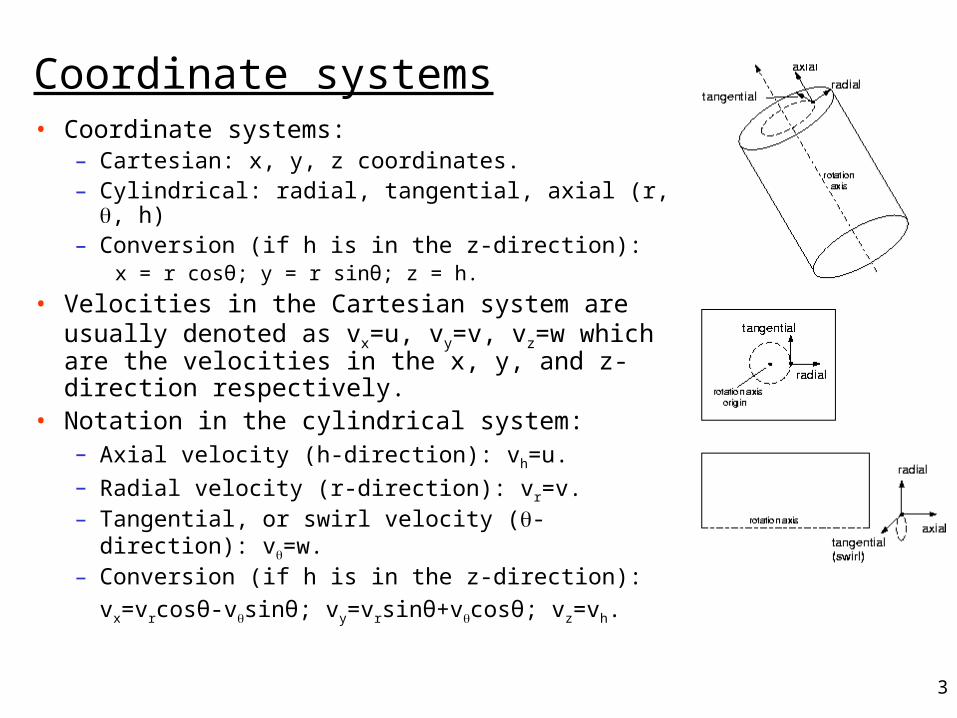
Coordinate systems• Coordinate systems:

– Cartesian: x, y, z coordinates.– Cylindrical: radial, tangential, axial (r, , h)– Conversion (if h is in the z-direction):

x = r cosθ; y = r sinθ; z = h.

• Velocities in the Cartesian system are usually denoted as vx=u, vy=v, vz=w which are the velocities in the x, y, and z-direction respectively.

• Notation in the cylindrical system:– Axial velocity (h-direction): vh=u.– Radial velocity (r-direction): vr=v.– Tangential, or swirl velocity (-direction): v=w.– Conversion (if h is in the z-direction):

vx=vrcosθ-vsinθ; vy=vrsinθ+vcosθ; vz=vh.

4

What can you calculate?• Flow field:

– Pumping rate.– Average velocities in fluid bulk, and important locations, such as

near feeds, at the bottom, around cooling coils.

• Pressure field:– Most commonly used to calculate impeller torque and power draw.– Other forces: such as on baffles.

• Additional physics:– Particle tracking.– Mixing times, RTD.– Temperature.– Species mixing.– Reactions.– Multiphase flow, such as solids suspension, or gas dispersion.

5

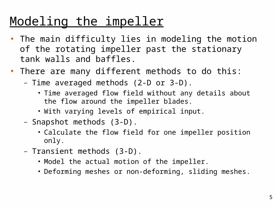
Modeling the impeller• The main difficulty lies in modeling the motion of the rotating

impeller past the stationary tank walls and baffles.

• There are many different methods to do this:– Time averaged methods (2-D or 3-D).

• Time averaged flow field without any details about the flow around the impeller blades.

• With varying levels of empirical input.

– Snapshot methods (3-D).• Calculate the flow field for one impeller position only.

– Transient methods (3-D).• Model the actual motion of the impeller.

• Deforming meshes or non-deforming, sliding meshes.

6

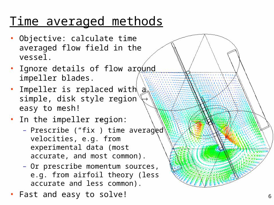
Time averaged methods• Objective: calculate time averaged flow

field in the vessel.

• Ignore details of flow around impeller blades.

• Impeller is replaced with a simple, disk style region easy to mesh!

• In the impeller region:– Prescribe (“fix”) time averaged

velocities, e.g. from experimental data (most accurate, and most common).

– Or prescribe momentum sources, e.g. from airfoil theory (less accurate and less common).

• Fast and easy to solve!

7

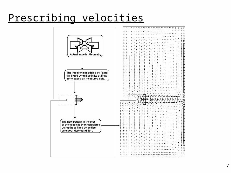
Prescribing velocities

8

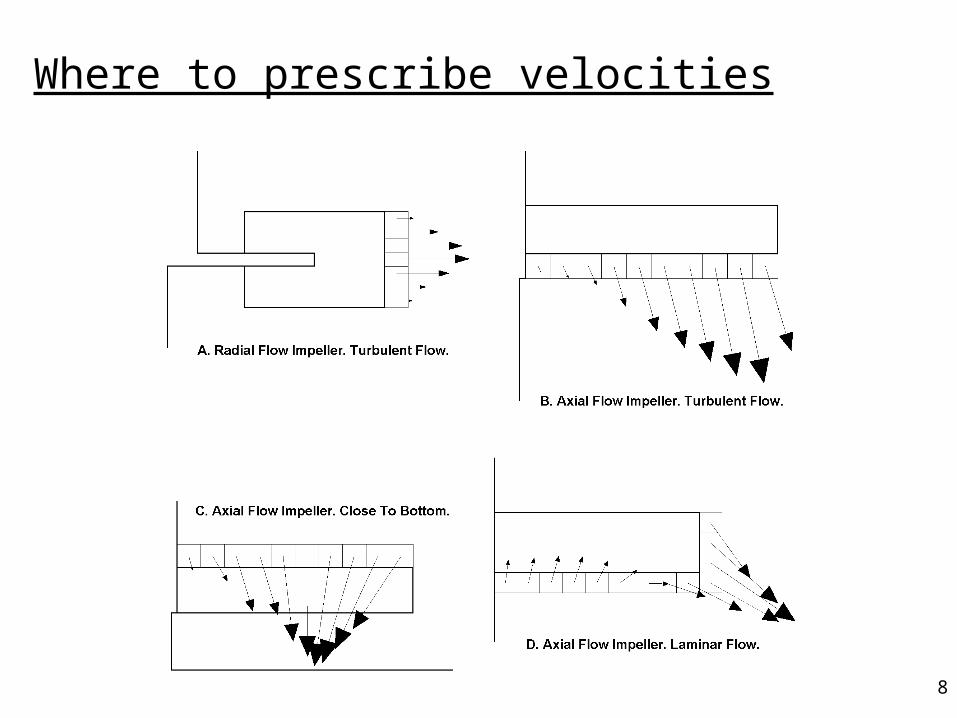
Where to prescribe velocities

9

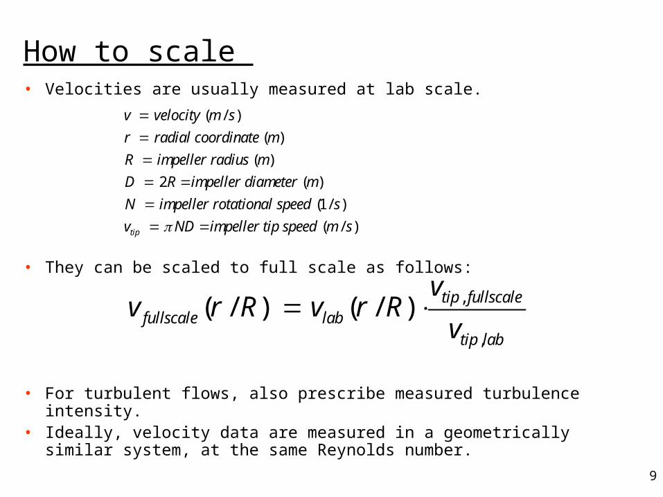
How to scale • Velocities are usually measured at lab scale.

• They can be scaled to full scale as follows:

• For turbulent flows, also prescribe measured turbulence intensity.• Ideally, velocity data are measured in a geometrically similar system, at

the same Reynolds number.

( / )

( )

( )

2 ( )

(1/ )

( / )tip

v velocity m s

r radial coordinate m

R impeller radius m

D R impeller diameter m

N impeller rotational speed s

v ND impeller tip speed m s

,

,

( / ) ( / ) tip fullscalefullscale lab

tip lab

vv r R v r R

v

10

When to use a time averaged method• It is the only impeller modeling method suitable for 2-D

calculations.

• The main advantages for 3-D calculations are:– Easy meshing with fewer cells than other methods.– Fast flow field calculations.– Fast species mixing and particle tracking calculations.

• The main disadvantage is:– You need velocity data for the particular impeller at the particular

Reynolds number. Note: this data can come from experiment or other CFD simulations.

– Hard to use for multiphase flows (e.g. gas-liquid flows).

• When is it useful: if you want to do many parametric reaction studies for the same system.

11

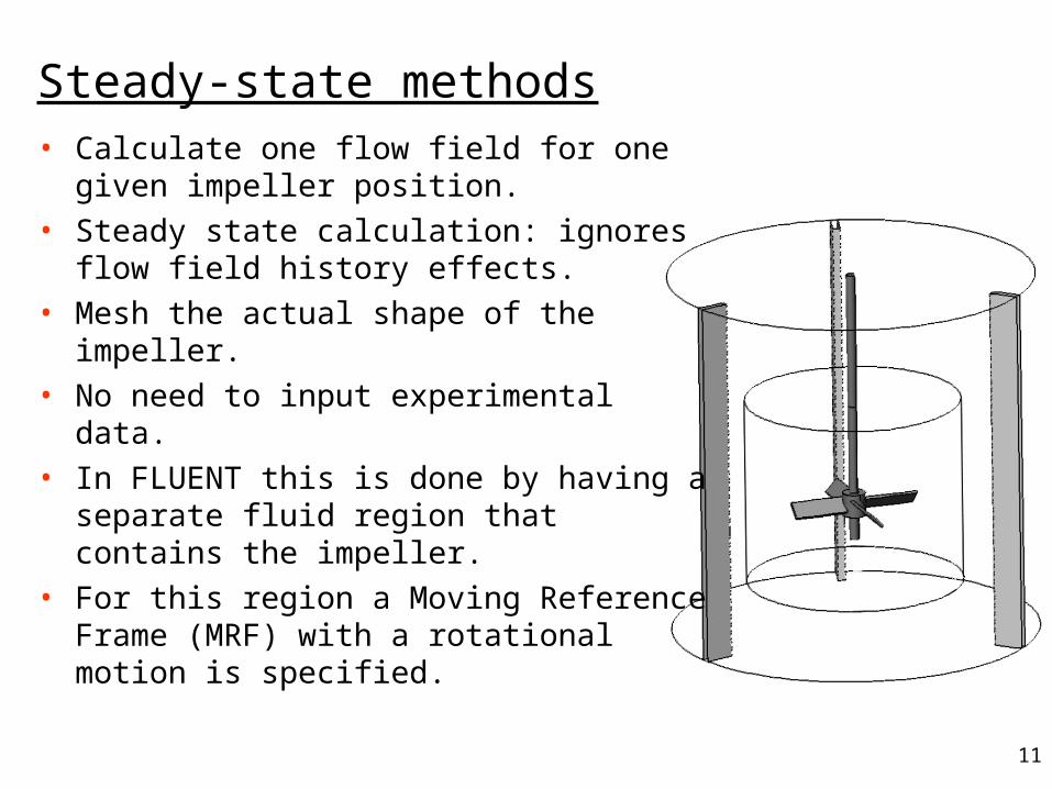
Steady-state methods• Calculate one flow field for one given

impeller position.

• Steady state calculation: ignores flow field history effects.

• Mesh the actual shape of the impeller.

• No need to input experimental data.

• In FLUENT this is done by having a separate fluid region that contains the impeller.

• For this region a Moving Reference Frame (MRF) with a rotational motion is specified.

12

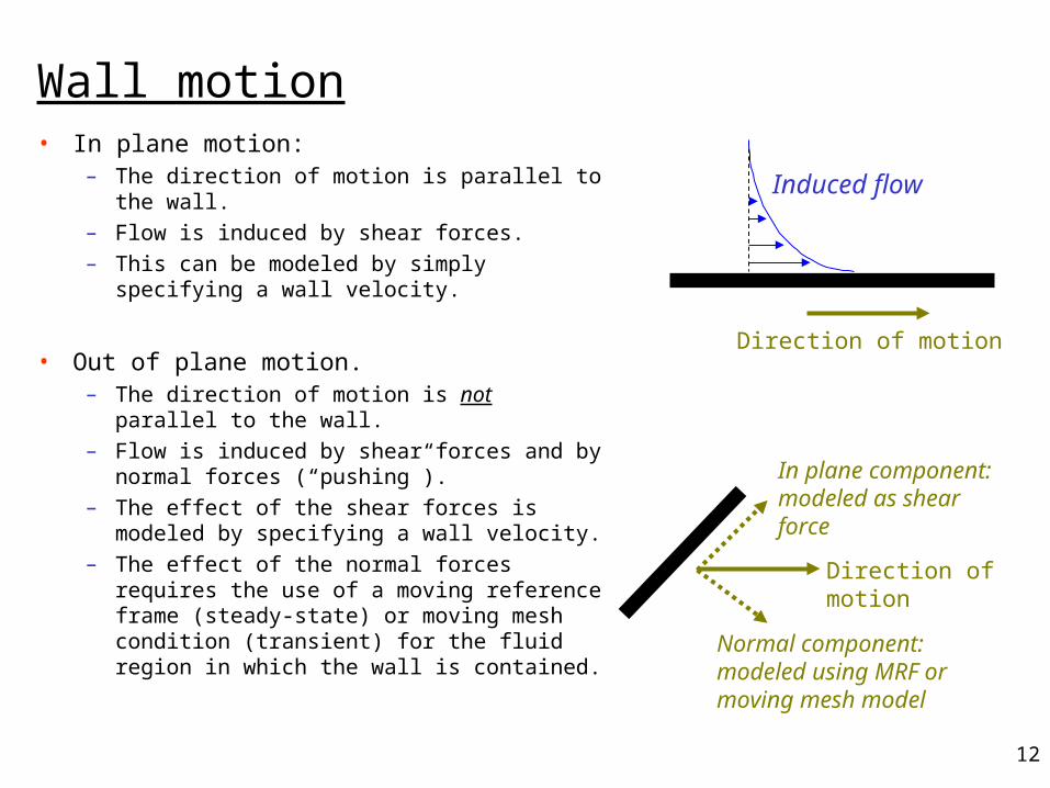
Wall motion• In plane motion:

– The direction of motion is parallel to the wall.– Flow is induced by shear forces.– This can be modeled by simply specifying a

wall velocity.

• Out of plane motion.– The direction of motion is not parallel to the

wall.– Flow is induced by shear forces and by

normal forces (“pushing”).– The effect of the shear forces is modeled by

specifying a wall velocity.– The effect of the normal forces requires the

use of a moving reference frame (steady-state) or moving mesh condition (transient) for the fluid region in which the wall is contained.

Direction of motion

Induced flow

Direction of motion

In plane component: modeled as shear force

Normal component: modeled using MRF or moving mesh model

13

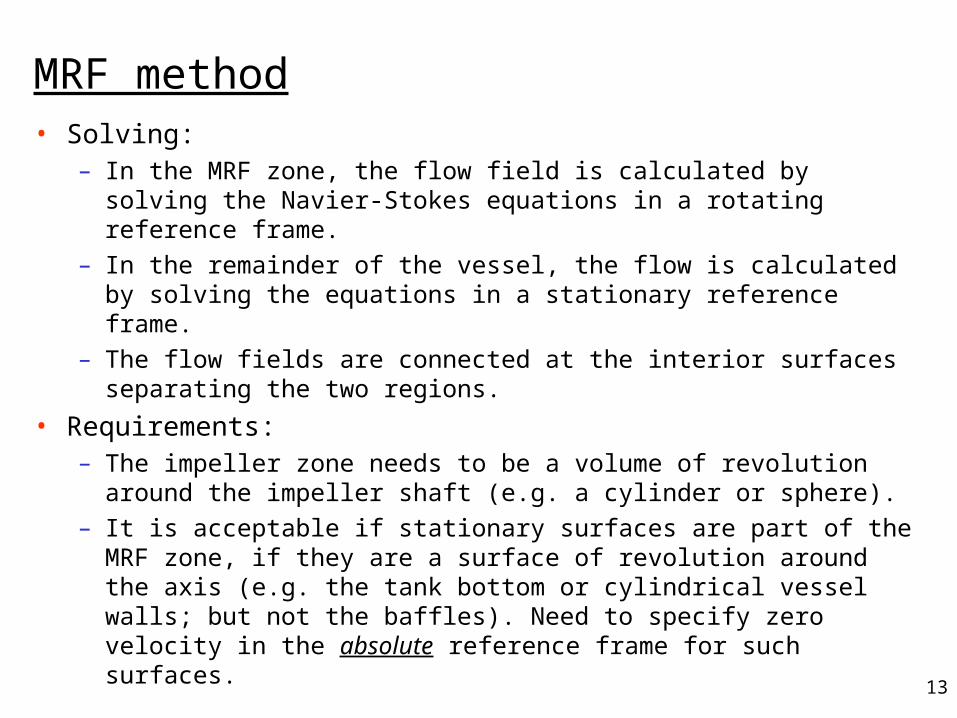
MRF method• Solving:

– In the MRF zone, the flow field is calculated by solving the Navier-Stokes equations in a rotating reference frame.

– In the remainder of the vessel, the flow is calculated by solving the equations in a stationary reference frame.

– The flow fields are connected at the interior surfaces separating the two regions.

• Requirements: – The impeller zone needs to be a volume of revolution around the

impeller shaft (e.g. a cylinder or sphere). – It is acceptable if stationary surfaces are part of the MRF zone, if

they are a surface of revolution around the axis (e.g. the tank bottom or cylindrical vessel walls; but not the baffles). Need to specify zero velocity in the absolute reference frame for such surfaces.

14

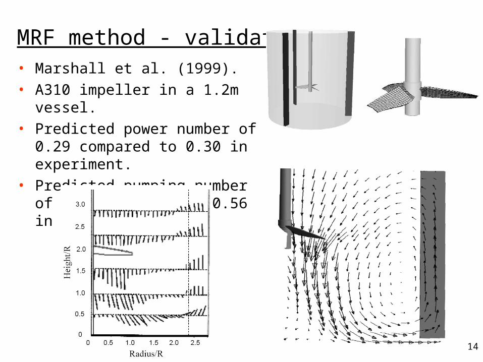
MRF method - validation• Marshall et al. (1999).

• A310 impeller in a 1.2m vessel.

• Predicted power number of 0.29 compared to 0.30 in experiment.

• Predicted pumping number of 0.52 compared to 0.56 in experiment.

15

When to use MRF• When experimental impeller data is not available.

• When the impeller geometry is known.

• When relatively short calculation times are desired.

• When transient flow field effects are not important:– Impellers on a central shaft in an unbaffled cylindrical vessel.– In baffled vessels when impeller-baffle interaction effects are of

minor importance.

16

Unsteady methods• A full time-dependent calculation is performed.

• Mesh the actual shape of the impeller.

• During the calculations, the impeller actually moves with respect to the stationary geometry components, such as the baffles.

• Because the geometry changes during the calculations, the mesh has to change as well.

• How to do this:– Moving/deforming mesh (MDM) method: Have one mesh, and

deform or remesh this every time step for the new impeller position.– Overset mesh method: Have a mesh for the solid geometry of the

impeller, move this through the stationary mesh for the fluid, and calculate intersections every time step.

– Sliding mesh method (called Moving Mesh in FLUENT).

17

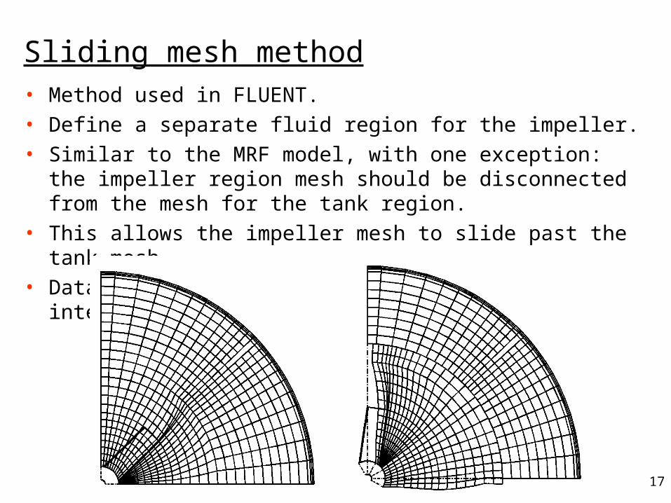
Sliding mesh method• Method used in FLUENT.

• Define a separate fluid region for the impeller.

• Similar to the MRF model, with one exception: the impeller region mesh should be disconnected from the mesh for the tank region.

• This allows the impeller mesh to slide past the tank mesh.

• Data is interchanged by defining grid interfaces.

18

When to use the sliding mesh method• Advantages:

– Fewest assumptions: suitable for widest range of cases.– Time-dependent solution is good for:

• Impeller-baffle interaction.

• Start-up or periodic transient flow details.

• Disadvantages:– CPU intensive.– Requires many cycles to reach “steady-state”.– Time scales for sliding mesh may not be compatible with time scales

of other processes (blending, solid suspension, etc.).

• Use when:– When there is strong interaction between impeller and walls or

baffles (e.g. systems with off-center or angled shafts).– Certain species or particle tracking calculations.

19

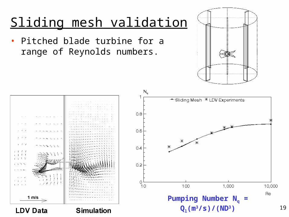
Sliding mesh validation• Pitched blade turbine for a range of

Reynolds numbers.

Pumping Number Nq = Ql(m3/s)/(ND3)

20

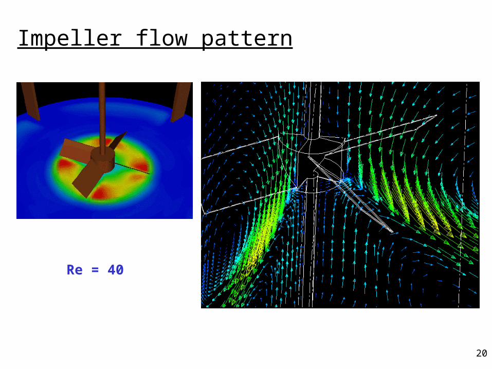
Impeller flow pattern

Re = 40

21

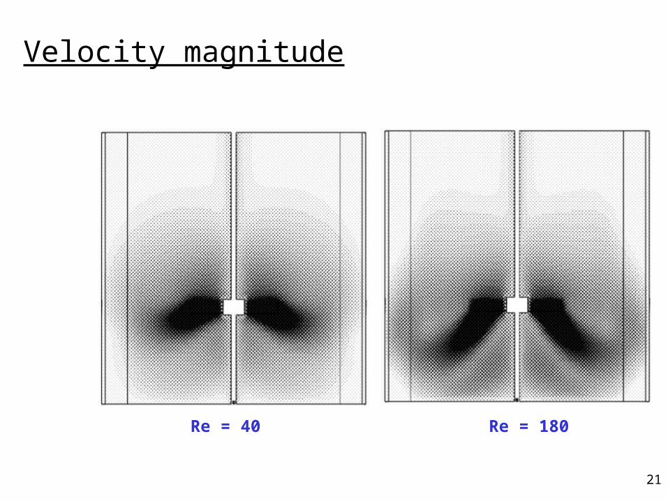
Velocity magnitude

Re = 40 Re = 180

22

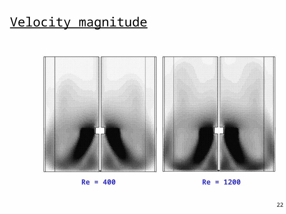
Velocity magnitude

Re = 400 Re = 1200

23

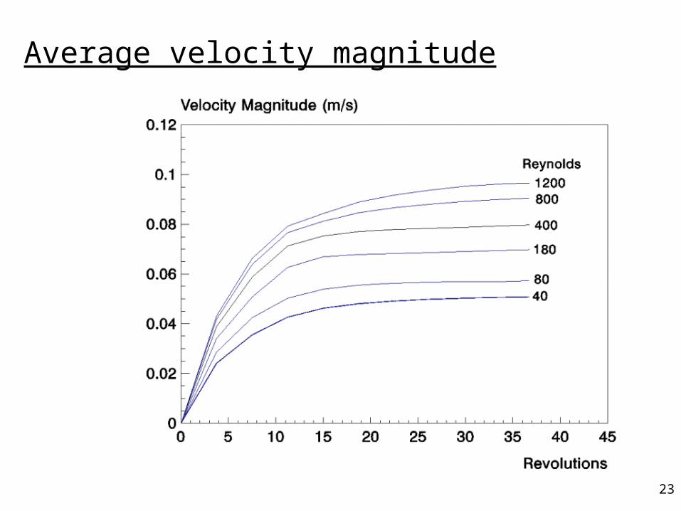
Average velocity magnitude

24

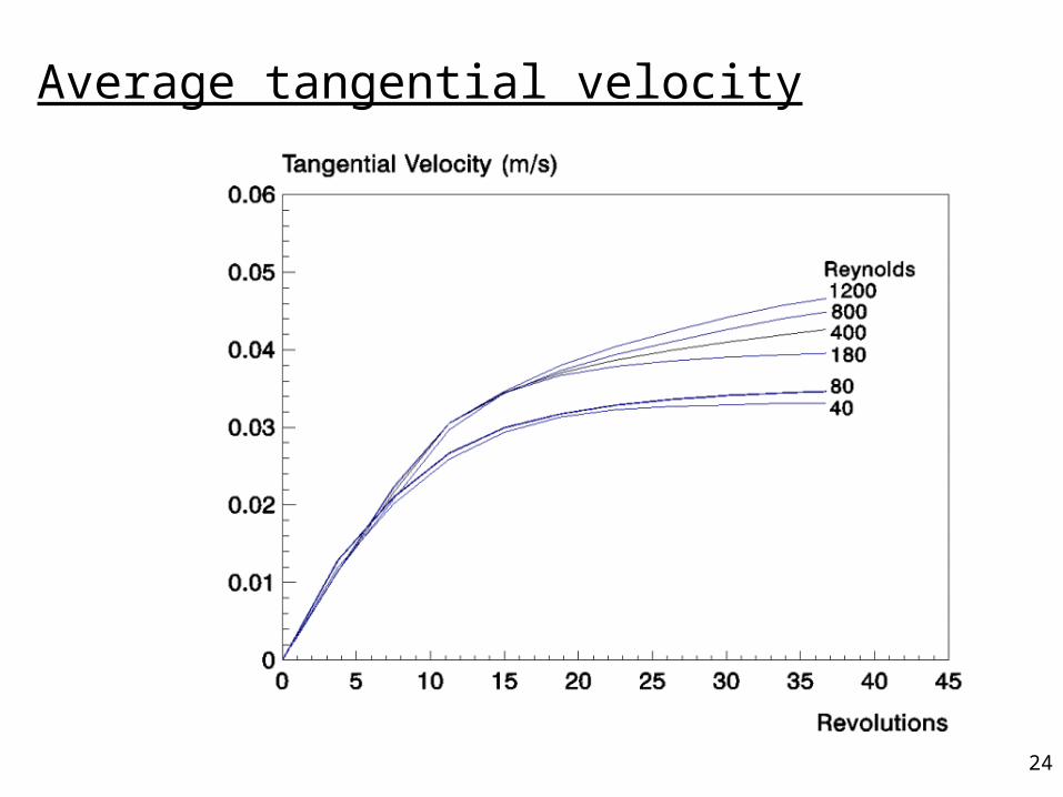
Average tangential velocity

25

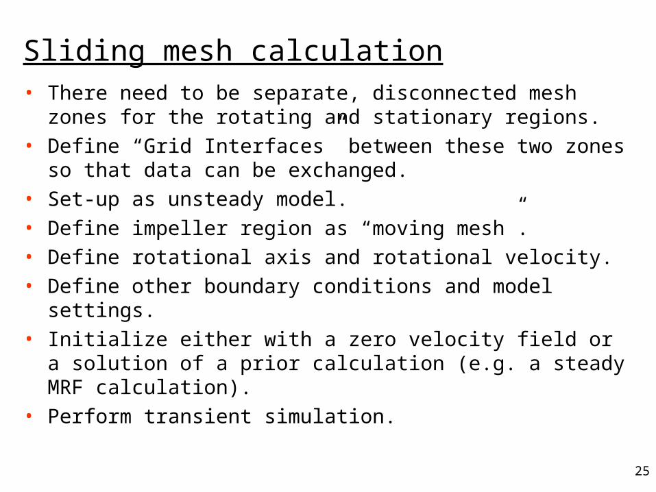
Sliding mesh calculation• There need to be separate, disconnected mesh zones for the

rotating and stationary regions.

• Define “Grid Interfaces” between these two zones so that data can be exchanged.

• Set-up as unsteady model.

• Define impeller region as “moving mesh”.

• Define rotational axis and rotational velocity.

• Define other boundary conditions and model settings.

• Initialize either with a zero velocity field or a solution of a prior calculation (e.g. a steady MRF calculation).

• Perform transient simulation.

26

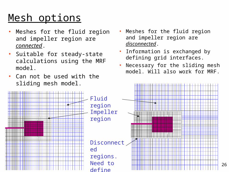
Mesh options• Meshes for the fluid region and

impeller region are connected.• Suitable for steady-state

calculations using the MRF model.

• Can not be used with the sliding mesh model.

• Meshes for the fluid region and impeller region are disconnected.

• Information is exchanged by defining grid interfaces.

• Necessary for the sliding mesh model. Will also work for MRF.

Fluid region

Impeller region

Disconnected regions. Need to define grid interfaces.

27

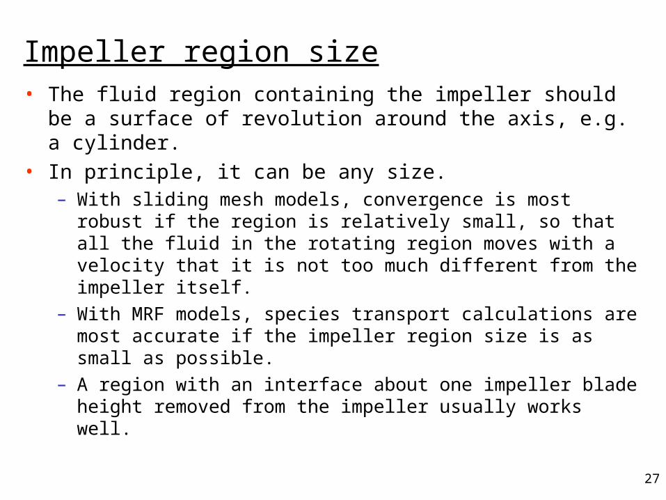
Impeller region size• The fluid region containing the impeller should be a surface of

revolution around the axis, e.g. a cylinder.

• In principle, it can be any size.– With sliding mesh models, convergence is most robust if the region

is relatively small, so that all the fluid in the rotating region moves with a velocity that it is not too much different from the impeller itself.

– With MRF models, species transport calculations are most accurate if the impeller region size is as small as possible.

– A region with an interface about one impeller blade height removed from the impeller usually works well.

28

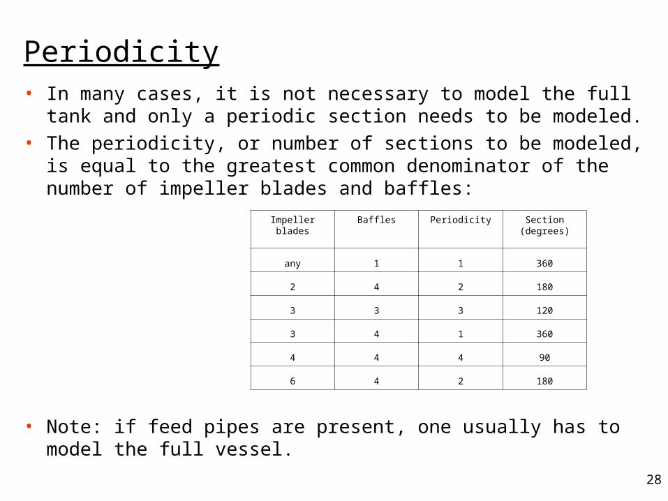
Periodicity• In many cases, it is not necessary to model the full tank and only

a periodic section needs to be modeled.

• The periodicity, or number of sections to be modeled, is equal to the greatest common denominator of the number of impeller blades and baffles:

• Note: if feed pipes are present, one usually has to model the full vessel.

Impeller blades Baffles Periodicity Section (degrees)

any 1 1 360

2 4 2 180

3 3 3 120

3 4 1 360

4 4 4 90

6 4 2 180

29

Liquid surface• The liquid surface usually deforms as a result of the liquid motion.

• If the deformation is large, and strong surface vortices form, air may be entrained from the headspace. – This may or may not be desirable.– Usually the system is designed to prevent this.

• In most baffled vessels, this deformation is usually small compared to the scale of the vessel.

• The liquid surface can in most cases be modeled as flat and frictionless (e.g. with a zero-shear or symmetry boundary condition).

• For systems where surface deformation is important, a free-surface multiphase model (e.g. VOF) has to be used.– This is very CPU time intensive and should be avoided if possible.

30

Model setup and convergence• Turbulence models:

– Unbaffled vessels: always use the Reynolds stress model (RSM).– Baffled vessels: the k- realizable model works well for most flows.

• Numerics:– Always use second order or higher numerics for the final solution.– For tetrahedral meshes, use the node-based gradient scheme.

• Initialization:– Initialize velocities to zero (in absolute reference frame).– Initialize k and to lower values than FLUENT default, e.g. 0.01 and

0.001 respectively (instead of 1).

• Convergence:– Default residual convergence criteria are usually not tight enough.– Monitor torque (moment) on the impeller, average tangential

velocity, and average velocity magnitude.

31

Flow field results• Flow field can be visualized by means of vector plots, contour

plots, iso-surfaces and pathlines.– Quickly shows if the number of impellers is sufficient.– Shows if material from feed pipes will go to the impeller or not.

• Quantitative data that can be extracted from the flow field and used in standard design procedures is:– Impeller torque and power draw.– Impeller pumping rate.– Shear rates, and effective viscosities.– Average velocities, and local velocities in regions of interest.

32

• Calculate power number of the impeller:– Either as data needed for your other analysis.– Or, if already known, as validation of the simulation result.

• Calculate power draw from the torque M(Nm) on the impeller (in FLUENT called the moment:

• And calculate the power number Po:

• Note: in principle the power draw can also be calculated as the volume integral of the energy dissipation rate , but this is usually less reliable.

3 1 3 5

( )Po

( ) ( ) ( )

P W

kg m N s D m

The power number

1( ) 2 ( ) ( )P W N s M Nm

33

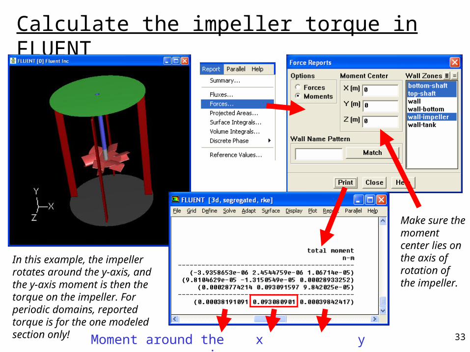
Calculate the impeller torque in FLUENT

Moment around the x y z axis

In this example, the impeller rotates around the y-axis, and the y-axis moment is then the torque on the impeller. For periodic domains, reported torque is for the one modeled section only!

Make sure the moment center lies on the axis of rotation of the impeller.

34

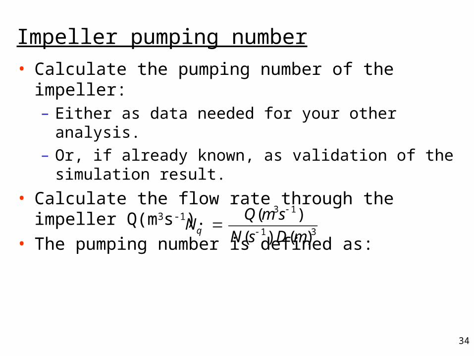
Impeller pumping number

• Calculate the pumping number of the impeller:– Either as data needed for your other analysis.– Or, if already known, as validation of the simulation

result.

• Calculate the flow rate through the impeller Q(m3s-1).

• The pumping number is defined as: 3 1

1 3

( )

( ) ( )q

Q m sN

N s D m

35

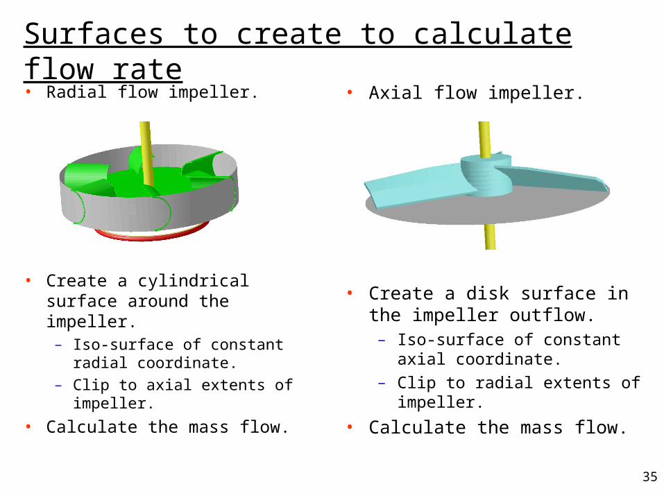
Surfaces to create to calculate flow rate• Radial flow impeller.

• Create a cylindrical surface around the impeller.– Iso-surface of constant radial

coordinate.

– Clip to axial extents of impeller.

• Calculate the mass flow.

• Axial flow impeller.

• Create a disk surface in the impeller outflow.– Iso-surface of constant axial

coordinate.

– Clip to radial extents of impeller.

• Calculate the mass flow.

36

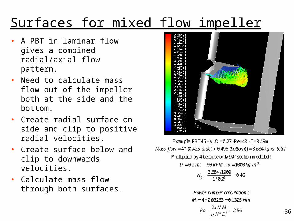
Surfaces for mixed flow impeller• A PBT in laminar flow gives a

combined radial/axial flow pattern.

• Need to calculate mass flow out of the impeller both at the side and the bottom.

• Create radial surface on side and clip to positive radial velocities.

• Create surface below and clip to downwards velocities.

• Calculate mass flow through both surfaces.

o

3

3

Example: PBT45 - W/D =0.27 -Re=40 - T=0.49m

4*(0.425 ( ) 0.496 ( )) 3.684 /

Multiplied by 4 because only 90 section modeled!

0.2 ; 60 ; 1000 /

3.684 /10000.46

1*0.2q

Mass flow side bottom kg s total

D m RPM kg m

N

Power number calculatio

3 5

:

4*0.03263 0.1305

22.56

n

M Nm

N MPo

N D

37

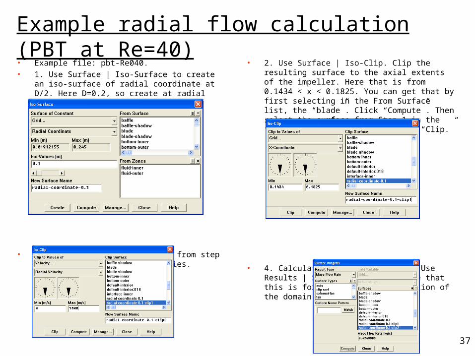
Example radial flow calculation (PBT at Re=40)• Example file: pbt-Re040.• 1. Use Surface | Iso-Surface to create an iso-surface of

radial coordinate at D/2. Here D=0.2, so create at radial coordinate=0.1.

• 3. Clip the surface resulting from step 2, to positive radial velocities.

• 2. Use Surface | Iso-Clip. Clip the resulting surface to the axial extents of the impeller. Here that is from 0.1434 < x < 0.1825. You can get that by first selecting in the From Surface list, the “blade”. Click “Compute”. Then select the surface from Step 1 in the “From Surface” list and then use “Clip.”

• 4. Calculate the Mass Flow Rate. Use Results | Surface Integrals. Note that this is for the one periodic section of the domain only.

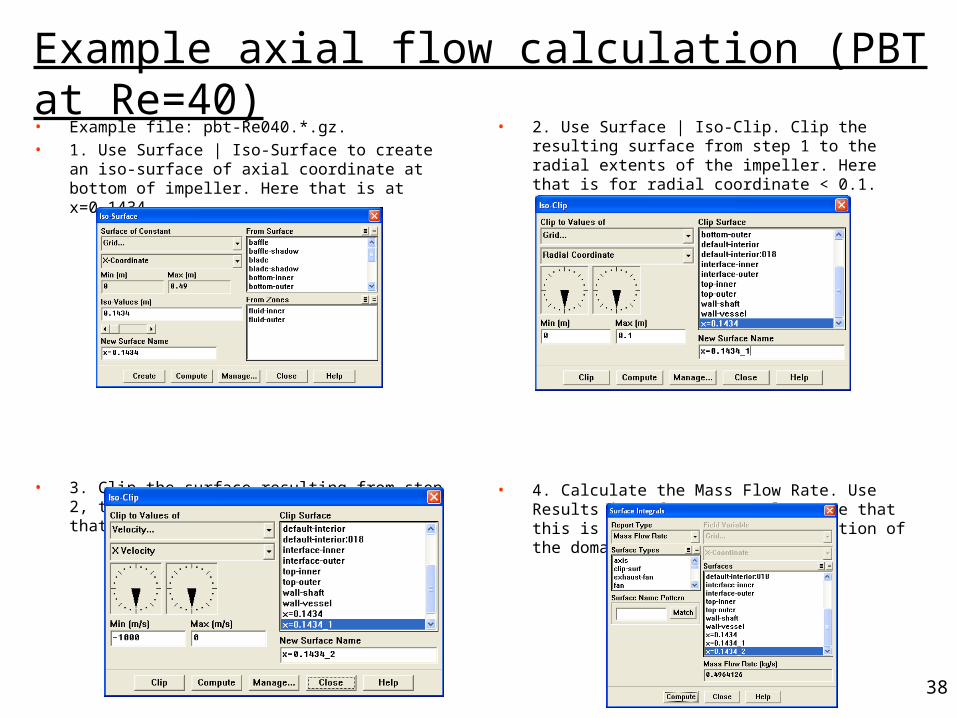
38

• 2. Use Surface | Iso-Clip. Clip the resulting surface from step 1 to the radial extents of the impeller. Here that is for radial coordinate < 0.1.

• 4. Calculate the Mass Flow Rate. Use Results | Surface Integrals. Note that this is for the one periodic section of the domain only.

• Example file: pbt-Re040.*.gz.• 1. Use Surface | Iso-Surface to create an iso-surface of

axial coordinate at bottom of impeller. Here that is at x=0.1434.

• 3. Clip the surface resulting from step 2, to downward axial velocities. Here that is for x-velocities < 0.

Example axial flow calculation (PBT at Re=40)

39

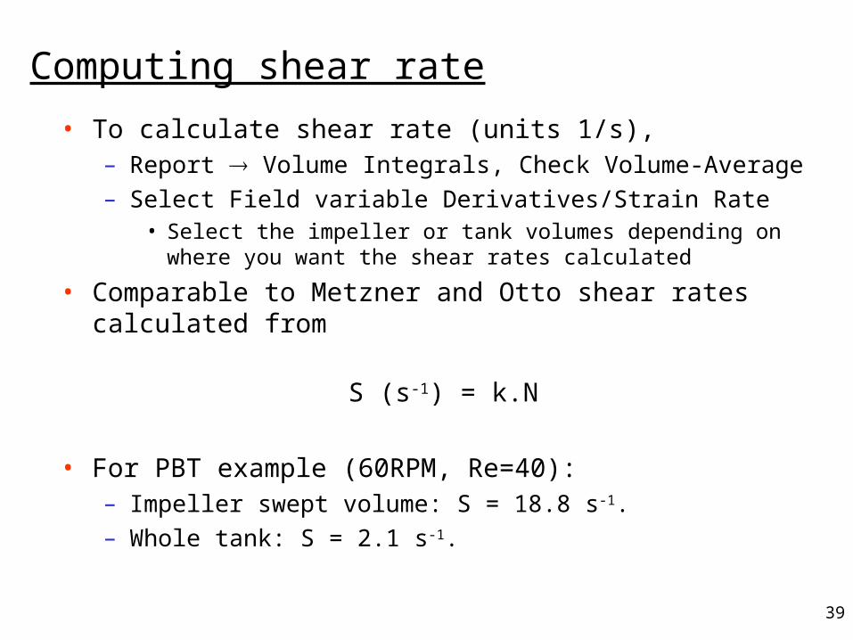
Computing shear rate

• To calculate shear rate (units 1/s), – Report Volume Integrals, Check Volume-Average– Select Field variable Derivatives/Strain Rate

• Select the impeller or tank volumes depending on where you want the shear rates calculated

• Comparable to Metzner and Otto shear rates calculated from

S (s-1) = k.N

• For PBT example (60RPM, Re=40):– Impeller swept volume: S = 18.8 s-1.– Whole tank: S = 2.1 s-1.

40

Conclusion• Main problem is the modeling of the impeller.

• Different impeller models are available.– Time averaged (e.g. “fix velocity”)– Steady state MRF.– Unsteady sliding mesh.

• In addition to flow fields, parameters needed as inputs to empirical correlations can be obtained:– Power number.– Pumping number.– Shear rates.