1 Introduction to quantum mechanics · 1 Introduction to quantum mechanics Quantum mechanics is the basic tool needed to describe, understand and devise NMR experiments. Fortunately

1–1

1 Introduction to quantum mechanics

Quantum mechanics is the basic tool needed to describe, understand and deviseNMR experiments. Fortunately for NMR spectroscopists, the quantummechanics of nuclear spins is quite straightforward and many usefulcalculations can be done by hand, quite literally "on the back of an envelope".This simplicity comes about from the fact that although there are a very largenumber of molecules in an NMR sample they are interacting very weakly withone another. Therefore, it is usually adequate to think about only one moleculeat a time. Even in one molecule, the number of spins which are interactingsignificantly with one another (i.e. are coupled) is relatively small, so thenumber of possible quantum states is quite limited.

The discussion will begin with revision of some mathematical conceptsfrequently encountered in quantum mechanics and NMR.

0DWKHPDWLFDOFRQFHSWV

1.1.1 Complex numbers

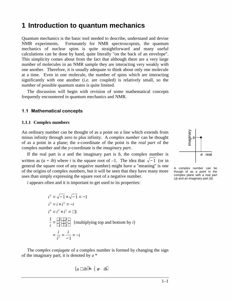
An ordinary number can be thought of as a point on a line which extends fromminus infinity through zero to plus infinity. A complex number can be thoughtof as a point in a plane; the x-coordinate of the point is the real part of thecomplex number and the y-coordinate is the imaginary part.

If the real part is a and the imaginary part is b, the complex number is

written as (a + ib) where i is the square root of –1. The idea that − 1 (or ingeneral the square root of any negative number) might have a "meaning" is oneof the origins of complex numbers, but it will be seen that they have many moreuses than simply expressing the square root of a negative number.

i appears often and it is important to get used to its properties:

i

i i i i

i i i

i i

i

ii

i

i

ii

2

3 2

4 2 2

2

1 1 1

1

1 1

1

= − × − = −

= × = −

= × = +

=

= =−

= −

multiplying top and bottom by

The complex conjugate of a complex number is formed by changing the signof the imaginary part; it is denoted by a *

( ) ( )a ib a ib+ = −*

real

imag

inar

y

b

a

A complex number can bethough of as a point in thecomplex plane with a real part(a) and an imaginary part (b).

1–2

The square magnitude of a complex number C is denoted C 2 and is found

by multiplying C by its complex conjugate; C 2 is always real

( )

( )( )

if C a ib

C C C

a ib a ib

a b

= +

= ×= + −

= +

2

2 2

*

These various properties are used when manipulating complex numbers:

( ) ( ) ( ) ( )( ) ( ) ( ) ( )

( )( )

( )( )

( )( ) ( )

( )( )( )

( )( )( )

( ) ( )( )

addition:

multiplication:

division:

multiplying top and bottom by

a ib c id a c i b d

a ib c id ac bd i ad bc

a ib

c id

a ib

c id

c id

c idc id

a ib c id

c d

a ib c id

c d

ac bd i bc ad

c d

+ + + = + + ++ × + = − + +

++

=++

×++

+

=+ +

+=

+ −+

=+ + −

+

*

**

*2 2 2 2 2 2

Using these relationships it is possible to show that

( ) ( )C D E C D E× × × = × × ×K K* * * *

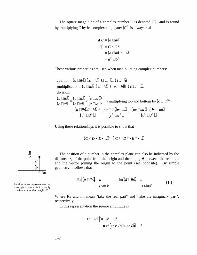
The position of a number in the complex plane can also be indicated by thedistance, r, of the point from the origin and the angle, θ, between the real axisand the vector joining the origin to the point (see opposite). By simplegeometry it follows that

( )[ ] ( )[ ]Re Im

cos sin

a ib a a ib b

r r

+ = + == =θ θ

[1.1]

Where Re and Im mean "take the real part" and "take the imaginary part",respectively.

In this representation the square amplitude is

( )

( )a ib a b

r r

+ = +

= + =

2 2 2

2 2 2 2cos sinθ θ

Re

Im

a

br

An alternative representation ofa complex number is to specifya distance, r, and an angle, θ.

1–3

where the identity cos2θ + sin2θ = 1 has been used.

1.1.2 Exponentials and complex exponentials

The exponential function, ex or exp(x), is defined as the power series

( )exp ! ! !x x x x= + + + +1 12

2 13

3 14

4 K

The number e is the base of natural logarithms, so that ln(e) = 1.Exponentials have the following properties

( ) ( ) ( ) ( ) ( )[ ] ( )( ) ( ) ( ) ( )

( ) ( )( )( ) ( ) ( )

exp exp exp exp exp exp

exp exp – exp exp

expexp

exp

expexp exp

0 1 2

0 1

1

2= × = + =

× = − = =

− = = × −

A B A B A A

A A A A

AA

A

BA B

The complex exponential is also defined in terms of a power series:

( ) ( ) ( ) ( )exp ! ! !i i i iθ θ θ θ= + + + +1 12

2 13

3 14

4K

By comparing this series expansion with those for sinθ and cosθ it can easilybe shown that

( )exp cos sini iθ θ θ= + [1.2]

This is a very important relation which will be used frequently. For negativeexponents there is a similar result

( ) ( ) ( )exp cos sin

cos sin

− = − + −= −

i i

i

θ θ θθ θ

[1.3]

where the identities ( )cos cos− =θ θ and ( )sin sin− = −θ θ have been used.

By comparison of Eqns. [1.1] and [1.2] it can be seen that the complexnumber (a + ib) can be written

( ) ( )a ib r i+ = exp θ

where r = a2 + b2 and tanθ = (b/a).

1–4

In the complex exponential form, the complex conjugate is found bychanging the sign of the term in i

( )( )

if

then

C r i

C r i

== −exp

* exp

θθ

It follows that

( ) ( )( ) ( )

C CC

r i r i

r i i r

r

2

2 2

2

0

== −

= − =

=

*

exp exp

exp exp

θ θθ θ

Multiplication and division of complex numbers in the (r,θ) format isstraightforward

( ) ( )

( ) ( ) ( )( )( )( ) ( ) ( ) ( )( )

let and thenC r i D s i

C r i ri C D rs i

C

D

r i

s i

r

si i

r

si

= =

= = − × = +

= = − = −

exp exp

expexp exp

exp

expexp exp exp

θ φ

θθ θ φ

θφ

θ φ θ φ

1 1 1

1.1.2.1 Relation to trigonometric functions

Starting from the relation

( )exp cos sini iθ θ θ= +

it follows that, as cos(–θ) = cosθ and sin(–θ) = – sinθ,

( )exp cos sin− = −i iθ θ θ

From these two relationships the following can easily be shown

( ) ( ) ( ) ( )[ ]( ) ( ) ( ) ( )[ ]

exp exp cos cos exp exp

exp exp sin sin exp exp

i i i i

i i i i ii

θ θ θ θ θ θ

θ θ θ θ θ θ

+ − = = + −

− − = = − −

2

2

12

12

or

or

1–5

1.1.3 Circular motion

In NMR basic form of motion is for magnetization to precess about a magneticfield. Viewed looking down the magnetic field, the tip of the magnetizationvector describes a circular path. It turns out that complex exponentials are avery convenient and natural way of describing such motion.

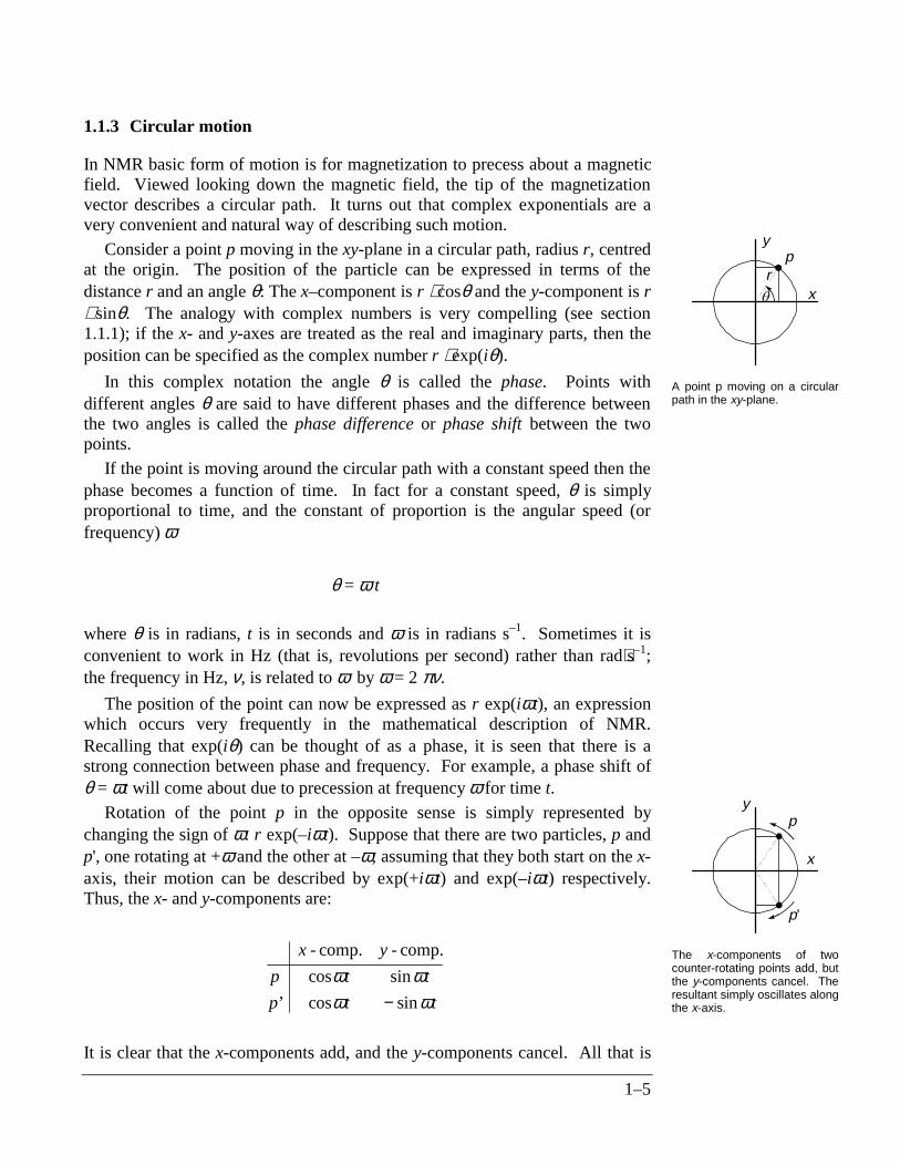
Consider a point p moving in the xy-plane in a circular path, radius r, centredat the origin. The position of the particle can be expressed in terms of thedistance r and an angle θ: The x–component is r ⋅ cosθ and the y-component is r⋅ sinθ. The analogy with complex numbers is very compelling (see section1.1.1); if the x- and y-axes are treated as the real and imaginary parts, then theposition can be specified as the complex number r ⋅ exp(iθ).

In this complex notation the angle θ is called the phase. Points withdifferent angles θ are said to have different phases and the difference betweenthe two angles is called the phase difference or phase shift between the twopoints.

If the point is moving around the circular path with a constant speed then thephase becomes a function of time. In fact for a constant speed, θ is simplyproportional to time, and the constant of proportion is the angular speed (orfrequency) ω

θ = ω t

where θ is in radians, t is in seconds and ω is in radians s–1. Sometimes it isconvenient to work in Hz (that is, revolutions per second) rather than rad⋅s–1;the frequency in Hz, ν, is related to ω by ω = 2 πν.

The position of the point can now be expressed as r exp(iωt), an expressionwhich occurs very frequently in the mathematical description of NMR.Recalling that exp(iθ) can be thought of as a phase, it is seen that there is astrong connection between phase and frequency. For example, a phase shift ofθ = ωt will come about due to precession at frequency ω for time t.

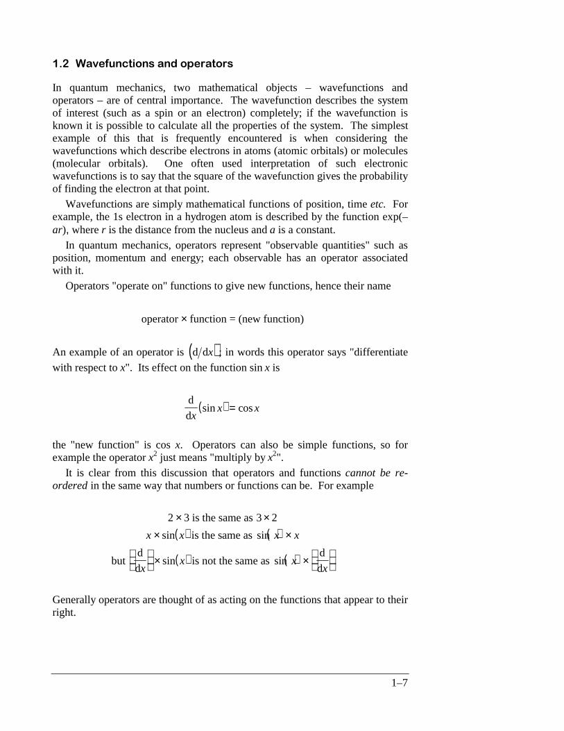
Rotation of the point p in the opposite sense is simply represented bychanging the sign of ω: r exp(–iωt). Suppose that there are two particles, p andp', one rotating at +ω and the other at –ω; assuming that they both start on the x-axis, their motion can be described by exp(+iωt) and exp(–iωt) respectively.Thus, the x- and y-components are:

x y

p t t

p t t

- comp. - comp.

cos sin

’ cos sin

ω ωω ω−

It is clear that the x-components add, and the y-components cancel. All that is

x

y

rp

A point p moving on a circularpath in the xy-plane.

x

yp

p’

The x-components of twocounter-rotating points add, butthe y-components cancel. Theresultant simply oscillates alongthe x-axis.

1–6

left is a component along the x-axis which is oscillating back and forth atfrequency ω. In the complex notation this result is easy to see as by Eqns. [1.2]and [1.3], exp(iω t) + exp( - iω t) = 2cosω t. In words, a point oscillating alonga line can be represented as two counter-rotating points.

1–7

:DYHIXQFWLRQVDQGRSHUDWRUV

In quantum mechanics, two mathematical objects – wavefunctions andoperators – are of central importance. The wavefunction describes the systemof interest (such as a spin or an electron) completely; if the wavefunction isknown it is possible to calculate all the properties of the system. The simplestexample of this that is frequently encountered is when considering thewavefunctions which describe electrons in atoms (atomic orbitals) or molecules(molecular orbitals). One often used interpretation of such electronicwavefunctions is to say that the square of the wavefunction gives the probabilityof finding the electron at that point.

Wavefunctions are simply mathematical functions of position, time etc. Forexample, the 1s electron in a hydrogen atom is described by the function exp(–ar), where r is the distance from the nucleus and a is a constant.

In quantum mechanics, operators represent "observable quantities" such asposition, momentum and energy; each observable has an operator associatedwith it.

Operators "operate on" functions to give new functions, hence their name

operator × function = (new function)

An example of an operator is ( )d dx ; in words this operator says "differentiate

with respect to x". Its effect on the function sin x is

( )d

dxx xsin cos=

the "new function" is cos x. Operators can also be simple functions, so forexample the operator x2 just means "multiply by x2".

It is clear from this discussion that operators and functions cannot be re-ordered in the same way that numbers or functions can be. For example

( ) ( )

( ) ( )

2 3 3 2× ×× ×

× ×

is the same as

is the same as

but d

d is not the same as

d

d

x x x x

xx x

x

sin sin

sin sin

Generally operators are thought of as acting on the functions that appear to theirright.

1–8

1.2.1 Eigenfunctions and eigenvalues

Generally, operators act on functions to give another function:

operator × function = (new function)

However, for a given operator there are some functions which, when actedupon, are regenerated, but multiplied by a constant

operator × function = constant × (function) [1.4]

Such functions are said to be eigenfunctions of the operator and the constantsare said to be the associated eigenvalues.

If the operator is $Q (the hat is to distinguish it as an operator) then Eqn.[1.4] can be written more formally as

$Qf qfq q= [1.5]

where fq is an eigenfunction of $Q with eigenvalue q; there may be more thatone eigenfunction each with different eigenvalues. Equation [1.5] is known asthe eigenvalue equation.

For example, is exp(ax), where a is a constant, an eigenfunction of the

operator ( )d dx ? To find out the operator and function are substituted into the

left-hand side of the eigenvalue equation, Eqn. [1.5]

( ) ( ) d

dxax a ax

=exp exp

It is seen that the result of operating on the function is to generate the originalfunction times a constant. Therefore exp(ax) is an eigenfunction of the operator

( )d dx with eigenvalue a.

Is sin(ax), where a is a constant, an eigenfunction of the operator ( )d dx ?

As before, the operator and function are substituted into the left-hand side of theeigenvalue equation.

( ) ( )

( )

d

d

constant

xax a ax

ax

=

≠ ×

sin cos

sin

1–9

As the original function is not regenerated, sin(ax) is not an eigenfunction of the

operator ( )d dx .

1.2.2 Normalization and orthogonality

A function, ψ, is said to be normalised if

( )ψ ψ τ*∫ =d 1

where, as usual, the * represents the complex conjugate. The notation dτ istaken in quantum mechanics to mean integration over the full range of allrelevant variables e.g. in three-dimensional space this would mean the range – ∞ to + ∞ for all of x, y and z.

Two functions ψ and φ are said to be orthogonal if

( )ψ φ τ*∫ =d 0

It can be shown that the eigenfunctions of an operator are orthogonal to oneanother, provided that they have different eigenvalues.

( )if and

then d

$ $

*

Qf qf Qf q f

f f

q q q q

q q

= = ′

=

′ ′

′∫ τ 0

1.2.3 Bra-ket notation

This short-hand notation for wavefunctions is often used in quantum mechanics.A wavefunction is represented by a "ket" K ; labels used to distinguishdifferent wavefunctions are written in the ket. For example

f q fq q is written or sometimes

It is a bit superfluous to write fq inside the ket.

The complex conjugate of a wavefunction is written as a "bra" K ; forexample

( )f qq ′ ′* is written

1–10

The rule is that if a bra appears on the left and a ket on the right, integrationover dτ is implied. So

( )′ ′∫q q f fq q implies d* τ

sometimes the middle vertical lines are merged: ′q q .

Although it takes a little time to get used to, the bra-ket notation is verycompact. For example, the normalization and orthogonality conditions can bewritten

q q q q= ′ =1 0

A frequently encountered integral in quantum mechanics is

ψ ψ τi jQ* $∫ d

where ψi and ψj are wavefunctions, distinguished by the subscripts i and j. Inbra-ket notation this integral becomes

i Q j$ [1.6]

as before, the presence of a bra on the left and a ket on the right impliesintegration over dτ. Note that in general, it is not allowed to re-order theoperator and the wavefunctions (section 1.2). The integral of Eqn. [1.6] is often

called a matrix element, specifically the ij element, of the operator $Q .

In the bra-ket notation the eigenvalue equation, Eqn. [1.5], becomes

$Q q q q=

Again, this is very compact.

1.2.4 Basis sets

The position of any point in three-dimensional space can be specified by givingits x-, y- and z-components. These three components form a completedescription of the position of the point; two components would be insufficientand adding a fourth component along another axis would be superfluous. Thethree axes are orthogonal to one another; that is any one axis does not have acomponent along the other two.

1–11

In quantum mechanics there is a similar idea of expressing a wavefunction interms of a set of other functions. For example, ψ may be expressed as a linearcombination of other functions

ψ = + + +a a a1 2 31 2 3 K

where the |i⟩ are called the basis functions and the ai are coefficients (numbers).Often there is a limited set of basis functions needed to describe any

particular wavefunction; such a set is referred to as a complete basis set.Usually the members of this set are orthogonal and can be chosen to benormalized, i.e.

i j i i= =0 1

1.2.5 Expectation values

A postulate of quantum mechanics is that if a system is described by awavefunction ψ then the value of an observable quantity represented by the

operator $Q is given by the expectation value, $Q , defined as

$* $

*Q

Q=

∫∫ψ ψ τ

ψ ψ τ

d

d

or in the bra-ket notation

$$

QQ

=ψ ψψ ψ

1–12

6SLQRSHUDWRUV

1.3.1 Spin angular momentum

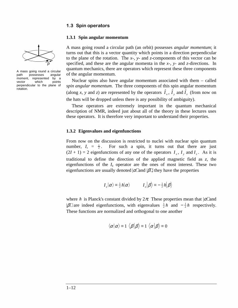
A mass going round a circular path (an orbit) possesses angular momentum; itturns out that this is a vector quantity which points in a direction perpendicularto the plane of the rotation. The x-, y- and z-components of this vector can bespecified, and these are the angular momenta in the x-, y- and z-directions. Inquantum mechanics, there are operators which represent these three componentsof the angular momentum.

Nuclear spins also have angular momentum associated with them – calledspin angular momentum. The three components of this spin angular momentum

(along x, y and z) are represented by the operators $ , $ $I I Ix y z and (from now on

the hats will be dropped unless there is any possibility of ambiguity).These operators are extremely important in the quantum mechanical

description of NMR, indeed just about all of the theory in these lectures usesthese operators. It is therefore very important to understand their properties.

1.3.2 Eigenvalues and eigenfunctions

From now on the discussion is restricted to nuclei with nuclear spin quantumnumber, I, = 1

2 . For such a spin, it turns out that there are just(2I + 1) = 2 eigenfunctions of any one of the operators I I Ix y z, and . As it is

traditional to define the direction of the applied magnetic field as z, theeigenfunctions of the Iz operator are the ones of most interest. These twoeigenfunctions are usually denoted |α⟩ and |β⟩; they have the properties

I Iz zα α β β= = −12

12h h

where h is Planck's constant divided by 2π. These properties mean that |α⟩ and|β⟩ are indeed eigenfunctions, with eigenvalues 1

2 h and − 12 h respectively.

These functions are normalized and orthogonal to one another

α α β β α β= = =1 1 0

p

A mass going round a circularpath possesses angularmoment, represented by avector which pointsperpendicular to the plane ofrotation.

1–13

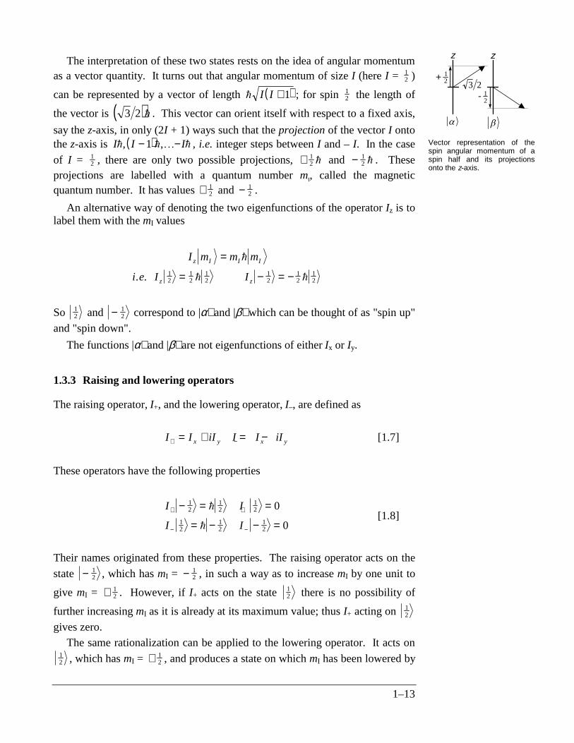
The interpretation of these two states rests on the idea of angular momentumas a vector quantity. It turns out that angular momentum of size I (here I = 1

2 )

can be represented by a vector of length ( )h I I + 1 ; for spin 12 the length of

the vector is ( )3 2 h . This vector can orient itself with respect to a fixed axis,

say the z-axis, in only (2I + 1) ways such that the projection of the vector I ontothe z-axis is ( )I I Ih h K h, ,− −1 , i.e. integer steps between I and – I. In the case

of I = 12 , there are only two possible projections, + 1

2 h and − 12 h . These

projections are labelled with a quantum number mI, called the magneticquantum number. It has values + 1

2 and − 12 .

An alternative way of denoting the two eigenfunctions of the operator Iz is tolabel them with the mI values

I m m m

i e I I

z I I I

z z

=

= − = −

h

h h. . 12

12

12

12

12

12

So 12 and − 1

2 correspond to |α⟩ and |β⟩ which can be thought of as "spin up"

and "spin down".

The functions |α⟩ and |β⟩ are not eigenfunctions of either Ix or Iy.

1.3.3 Raising and lowering operators

The raising operator, I+, and the lowering operator, I–, are defined as

I I iI I I iIx y x y+ −= + = − [1.7]

These operators have the following properties

I I

I I

+ +

− −

− = =

= − − =

12

12

12

12

12

12

0

0

h

h[1.8]

Their names originated from these properties. The raising operator acts on the

state − 12 , which has mI = − 1

2 , in such a way as to increase mI by one unit to

give mI = + 12 . However, if I+ acts on the state 1

2 there is no possibility of

further increasing mI as it is already at its maximum value; thus I+ acting on 12

gives zero.The same rationalization can be applied to the lowering operator. It acts on

12 , which has mI = + 1

2 , and produces a state on which mI has been lowered by

z z

12+

12-

3 2

Vector representation of thespin angular momentum of aspin half and its projectionsonto the z-axis.

1–14

one i.e. mI = − 12 . However, the mI value can be lowered no further so I– acting

on − 12 gives zero.

Using the definitions of Eqn. [1.7], Ix and Iy can be expressed in terms of theraising and lowering operators:

( ) ( )I I I I I Ix y i= + = −+ − + −12

12

Using these, and the properties given in Eqn. [1.8], it is easy to work out theeffect that Ix and Iy have on the states |α⟩ and |β⟩; for example

( )I I I

I I

x α αα α

β

β

= +

= +

= +

=

+ −

+ −

12

12

12

12

12

0 h

h

By a similar method it can be found that

I I I i I ix x y yα β β α α β β α= = = = −12

12

12

12h h h h [1.9]

These relationships all show that |α⟩ and |β⟩ are not eigenfunctions of Ix and Iy.

+DPLOWRQLDQV

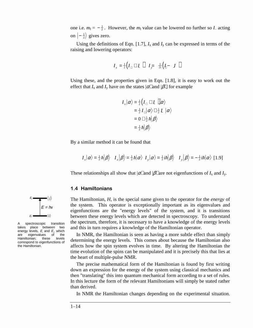
The Hamiltonian, H, is the special name given to the operator for the energy ofthe system. This operator is exceptionally important as its eigenvalues andeigenfunctions are the "energy levels" of the system, and it is transitionsbetween these energy levels which are detected in spectroscopy. To understandthe spectrum, therefore, it is necessary to have a knowledge of the energy levelsand this in turn requires a knowledge of the Hamiltonian operator.

In NMR, the Hamiltonian is seen as having a more subtle effect than simplydetermining the energy levels. This comes about because the Hamiltonian alsoaffects how the spin system evolves in time. By altering the Hamiltonian thetime evolution of the spins can be manipulated and it is precisely this that lies atthe heart of multiple-pulse NMR.

The precise mathematical form of the Hamiltonian is found by first writingdown an expression for the energy of the system using classical mechanics andthen "translating" this into quantum mechanical form according to a set of rules.In this lecture the form of the relevant Hamiltonians will simply be stated ratherthan derived.

In NMR the Hamiltonian changes depending on the experimental situation.

i

j

Ei

Ej

E = h ν

A spectroscopic transitiontakes place between twoenergy levels, Ei and Ej, whichare eigenvalues of theHamiltonian; these levelscorrespond to eigenfunctions ofthe Hamiltonian.

1–15

There is one Hamiltonian for the spin or spins in the presence of the appliedmagnetic field, but this Hamiltonian changes when a radio-frequency pulse isapplied.

1.4.1 Free precession

Free precession is when the spins experience just the applied magnetic field, B0,traditionally taken to be along the z-axis.

1.4.1.1 One spin

The free precession Hamiltonian, Hfree, is

Hfree = γB0hIz

where γ is the gyromagnetic ratio, a constant characteristic of a particularnuclear species such as proton or carbon-13. The quantity γB0h has the units ofenergy, which is expected as the Hamiltonian is the operator for energy.However, it turns out that it is much more convenient to write the Hamiltonianin units of angular frequency (radians s–1), which is achieved by dividing theexpression for Hfree by h to give

Hfree = γB0Iz

To be consistent it is necessary then to divide all of the operators by h. As aresult all of the factors of h disappear from many of the equations given abovee.g. they become:

I Iz zα α β β= = −12

12 [1.10]

I I+ −= =β α α βh [1.11]

I I I i I ix x y yα β β α α β β α= = = = −12

12

12

12 [1.12]

From now on, the properties of the wavefunctions and operators will be used inthis form. The quantity γB0, which has dimensions of angular frequency (rad s–

1), is often called the Larmor frequency, ω0.

Eigenfunctions and eigenvalues

The eigenfunctions and eigenvalues of Hfree are a set of functions, |i⟩, which

1–16

satisfy the eigenvalue equation:

H i i

I i ii

z i

free ==

εω ε0

It is already known that |α⟩ and |β⟩ are eigenfunctions of Iz, so it follows thatthey are also eigenfunctions of any operator proportional to Iz:

H I zfree α ω αω α

==

0

12 0

and likewise H I zfree β ω β ω β= = −012 0 .

So, |α⟩ and |β⟩ are eigenfunctions of Hfree with eigenvalues 12 0ω and − 12 0ω ,

respectively. These two eigenfunctions correspond to two energy levels and a

transition between them occurs at frequency ( )( )12 0

12 0 0ω ω ω− − = .

1.4.1.2 Several spins

If there is more then one spin, each simply contributes a term to Hfree;subscripts are used to indicate that the operator applies to a particular spin

H I Iz zfree = + +ω ω0 1 1 0 2 2, , K

where I1z is the operator for the first spin, I2z is that for the second and so on.Due to the effects of chemical shift, the Larmor frequencies of the spins may bedifferent and so they have been written as ω0,i.

Eigenfunctions and eigenvalues

As Hfree separates into a sum of terms, the eigenfunctions turn out to be aproduct of the eigenfunctions of the separate terms; as the eigenfunctions ofω0,1I1z are already known, it is easy to find those for the whole Hamiltonian.

As an example, consider the Hamiltonian for two spins

H I Iz zfree = +ω ω0 1 1 0 2 2, ,

From section 1.4.1.1, it is known that, for spin 1

1–17

ω α ω α ω β ω β0 1 1 112 0 1 0 1 1 1

12 0 2 1, , ,I Iz z= = −and

likewise for spin 2

ω α ω α ω β ω β0 2 2 212 0 2 2 0 2 2 2

12 0 2 2, , , ,I Iz z= = −and

Consider the function |β1⟩|α2⟩, which is a product of one of the eigenfunctionsfor spin 1 with one for spin 2. To show that this is an eigenfunction of Hfree, theHamiltonian is applied to the function

( )

( )

H I I

I I

I

z z

z z

z

free β α ω ω β α

ω β α ω β α

ω β α ω β α

ω β α ω β α

ω ω β α

1 2 0 1 1 0 2 2 1 2

0 1 1 1 2 0 2 2 1 2

12 0 1 1 2 0 2 1 2 2

12 0 1 1 2

12 0 2 1 2

12 0 1

12 0 2 1 2

= +

= +

= − +

= − +

= − +

, ,

, ,

, ,

, ,

, ,

As the action of Hfree on |β1⟩|α2⟩ is to regenerate the function, then it has beenshown that the function is indeed an eigenfunction, with eigenvalue

( )− +12 0 1

12 0 2ω ω, , . Some comment in needed on these manipulation needed

between lines 2 and 3 of the above calculation. The order of the function |β1⟩and the operator I2z were changed between lines 2 and 3. Generally, as wasnoted above, it is not permitted to reorder operators and functions; however it ispermitted in this case as the operator refers to spin 2 but the function refers tospin 1. The operator has no effect, therefore, on the function and so the two canbe re-ordered.

There are four possible products of the single-spin eigenfunctions and eachof these can be shown to be an eigenfunction. The table summarises the results;in it, the shorthand notation has been used in which |β1⟩|α2⟩ is denoted |βα⟩ i.e.it is implied by the order of the labels as to which spin they apply to

Eigenfunctions and eigenvalues for two spinseigenfunction mI,1 mI,2 M eigenvalue

αα + 12 + 1

21 + +1

2 0 112 0 2ω ω, ,

αβ + 12 − 1

20 + −1

2 0 112 0 2ω ω, ,

βα − 12 + 1

20 − +1

2 0 112 0 2ω ω, ,

ββ − 12 − 1

21 − −1

2 0 112 0 2ω ω, ,

1–18

Also shown in the table are the mI values for the individual spins and thetotal magnetic quantum number, M, which is simply the sum of the mI values ofthe two spins.

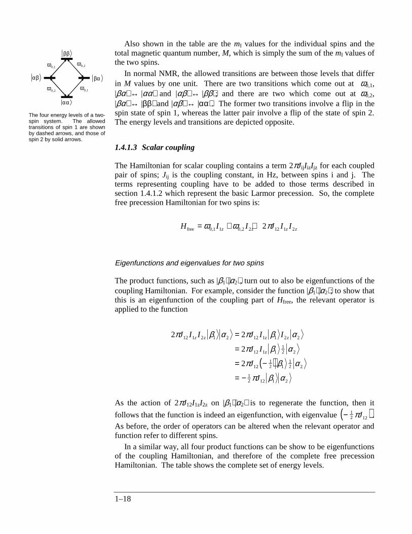
In normal NMR, the allowed transitions are between those levels that differin M values by one unit. There are two transitions which come out at ω0,1,|βα⟩ ↔ |αα⟩ and |αβ⟩ ↔ |ββ⟩; and there are two which come out at ω0,2,|βα⟩ ↔ |ββ⟩ and |αβ⟩ ↔ |αα⟩. The former two transitions involve a flip in thespin state of spin 1, whereas the latter pair involve a flip of the state of spin 2.The energy levels and transitions are depicted opposite.

1.4.1.3 Scalar coupling

The Hamiltonian for scalar coupling contains a term 2πJijIizIjz for each coupledpair of spins; Jij is the coupling constant, in Hz, between spins i and j. Theterms representing coupling have to be added to those terms described insection 1.4.1.2 which represent the basic Larmor precession. So, the completefree precession Hamiltonian for two spins is:

H I I J I Iz z z zfree = + +ω ω π0 1 1 0 2 2 12 1 22, ,

Eigenfunctions and eigenvalues for two spins

The product functions, such as |β1⟩|α2⟩, turn out to also be eigenfunctions of thecoupling Hamiltonian. For example, consider the function |β1⟩|α2⟩; to show thatthis is an eigenfunction of the coupling part of Hfree, the relevant operator isapplied to the function

( )

2 2

2

2

12 1 2 1 2 12 1 1 2 2

12 1 112 2

1212 1

12 2

12 12 1 2

π β α π β α

π β α

π β α

π β α

J I I J I I

J I

J

J

z z z z

z

=

=

= −

= −

As the action of 2πJ12I1zI2z on |β1⟩|α2⟩ is to regenerate the function, then it

follows that the function is indeed an eigenfunction, with eigenvalue ( )− 12 12πJ .

As before, the order of operators can be altered when the relevant operator andfunction refer to different spins.

In a similar way, all four product functions can be show to be eigenfunctionsof the coupling Hamiltonian, and therefore of the complete free precessionHamiltonian. The table shows the complete set of energy levels.

αβ

ββ

βα

αα

ω0 1,

ω0 1,

ω 0 2,

ω0 2,

The four energy levels of a two-spin system. The allowedtransitions of spin 1 are shownby dashed arrows, and those ofspin 2 by solid arrows.

1–19

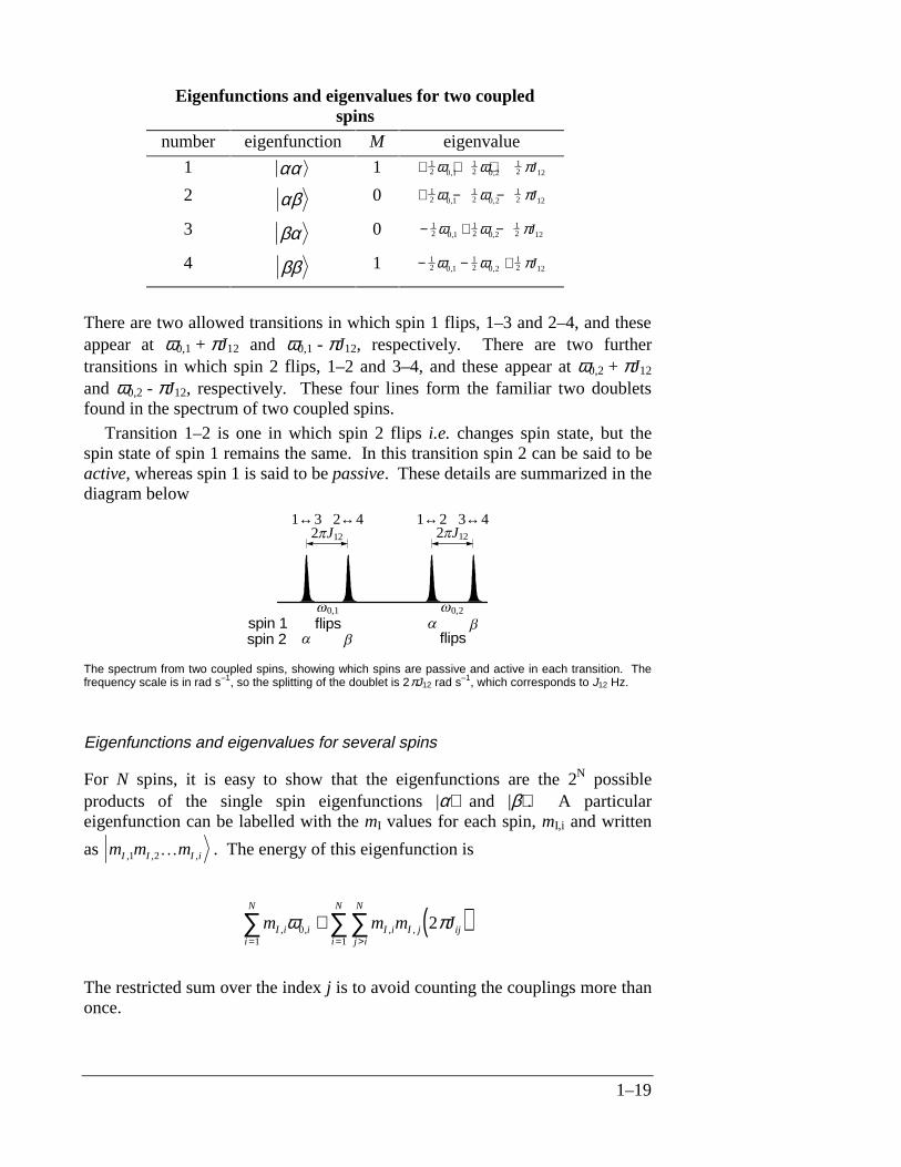
There are two allowed transitions in which spin 1 flips, 1–3 and 2–4, and theseappear at ω0,1 + πJ12 and ω0,1 - πJ12, respectively. There are two furthertransitions in which spin 2 flips, 1–2 and 3–4, and these appear at ω0,2 + πJ12

and ω0,2 - πJ12, respectively. These four lines form the familiar two doubletsfound in the spectrum of two coupled spins.

Transition 1–2 is one in which spin 2 flips i.e. changes spin state, but thespin state of spin 1 remains the same. In this transition spin 2 can be said to beactive, whereas spin 1 is said to be passive. These details are summarized in thediagram below

2 J122 J12

1↔3 2↔4 1↔2 3↔4

0,1 0,2

flipsflips

spin 1spin 2

The spectrum from two coupled spins, showing which spins are passive and active in each transition. Thefrequency scale is in rad s–1, so the splitting of the doublet is 2πJ12 rad s–1, which corresponds to J12 Hz.

Eigenfunctions and eigenvalues for several spins

For N spins, it is easy to show that the eigenfunctions are the 2N possibleproducts of the single spin eigenfunctions |α⟩ and |β⟩. A particulareigenfunction can be labelled with the mI values for each spin, mI,i and written

as m m mI I I i, , ,1 2K . The energy of this eigenfunction is

( )m m m JI ii

N

i I i I j ijj i

N

i

N

, , , ,= >=∑ ∑∑+

10

1

2ω π

The restricted sum over the index j is to avoid counting the couplings more thanonce.

Eigenfunctions and eigenvalues for two coupledspins

number eigenfunction M eigenvalue

1 αα 1 + + +12 0 1

12 0 2

12 12ω ω π, , J

2 αβ 0 + − −12 0 1

12 0 2

12 12ω ω π, , J

3 βα 0 − + −12 0 1

12 0 2

12 12ω ω π, , J

4 ββ 1 − − +12 0 1

12 0 2

12 12ω ω π, , J

1–20

1.4.2 Pulses

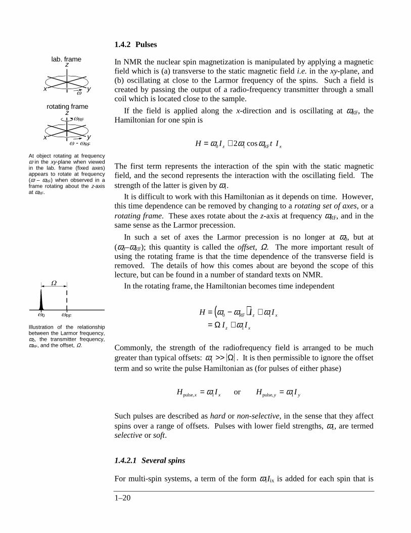
In NMR the nuclear spin magnetization is manipulated by applying a magneticfield which is (a) transverse to the static magnetic field i.e. in the xy-plane, and(b) oscillating at close to the Larmor frequency of the spins. Such a field iscreated by passing the output of a radio-frequency transmitter through a smallcoil which is located close to the sample.

If the field is applied along the x-direction and is oscillating at ωRF, theHamiltonian for one spin is

H I t Iz x= +ω ω ω0 12 cos RF

The first term represents the interaction of the spin with the static magneticfield, and the second represents the interaction with the oscillating field. Thestrength of the latter is given by ω1.

It is difficult to work with this Hamiltonian as it depends on time. However,this time dependence can be removed by changing to a rotating set of axes, or arotating frame. These axes rotate about the z-axis at frequency ωRF, and in thesame sense as the Larmor precession.

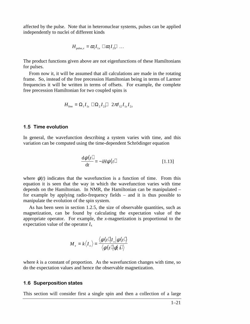
In such a set of axes the Larmor precession is no longer at ω0, but at(ω0–ωRF); this quantity is called the offset, Ω. The more important result ofusing the rotating frame is that the time dependence of the transverse field isremoved. The details of how this comes about are beyond the scope of thislecture, but can be found in a number of standard texts on NMR.

In the rotating frame, the Hamiltonian becomes time independent

( )H I I

I Iz x

z x

= − += +

ω ω ωω

0 1

1

RF

Ω

Commonly, the strength of the radiofrequency field is arranged to be muchgreater than typical offsets: ω1 >> Ω . It is then permissible to ignore the offsetterm and so write the pulse Hamiltonian as (for pulses of either phase)

H I H Ix x y ypulse, pulse,or= =ω ω1 1

Such pulses are described as hard or non-selective, in the sense that they affectspins over a range of offsets. Pulses with lower field strengths, ω1, are termedselective or soft.

1.4.2.1 Several spins

For multi-spin systems, a term of the form ω1Iix is added for each spin that is

lab. frame

x y

z

rotating frame

x y

zRF

- RF

At object rotating at frequencyω in the xy-plane when viewedin the lab. frame (fixed axes)appears to rotate at frequency(ω – ωRF) when observed in aframe rotating about the z-axisat ωRF.

0 RF

Illustration of the relationshipbetween the Larmor frequency,ω0, the transmitter frequency,ωRF, and the offset, Ω.

1–21

affected by the pulse. Note that in heteronuclear systems, pulses can be appliedindependently to nuclei of different kinds

H I Ix x xpulse, = + +ω ω1 1 1 2 K

The product functions given above are not eigenfunctions of these Hamiltoniansfor pulses.

From now it, it will be assumed that all calculations are made in the rotatingframe. So, instead of the free precession Hamiltonian being in terms of Larmorfrequencies it will be written in terms of offsets. For example, the completefree precession Hamiltonian for two coupled spins is

H I I J I Iz z z zfree = + +Ω Ω1 1 2 2 12 1 22π

7LPHHYROXWLRQ

In general, the wavefunction describing a system varies with time, and thisvariation can be computed using the time-dependent Schrödinger equation

( ) ( )d

d

ψψ

t

tiH t= − [1.13]

where ψ(t) indicates that the wavefunction is a function of time. From thisequation it is seen that the way in which the wavefunction varies with timedepends on the Hamiltonian. In NMR, the Hamiltonian can be manipulated –for example by applying radio-frequency fields – and it is thus possible tomanipulate the evolution of the spin system.

As has been seen in section 1.2.5, the size of observable quantities, such asmagnetization, can be found by calculating the expectation value of theappropriate operator. For example, the x-magnetization is proportional to theexpectation value of the operator Ix

( ) ( )( ) ( )

M k It I t

t tx x

x= =ψ ψ

ψ ψ

where k is a constant of proportion. As the wavefunction changes with time, sodo the expectation values and hence the observable magnetization.

6XSHUSRVLWLRQVWDWHV

This section will consider first a single spin and then a collection of a large

1–22

number of non-interacting spins, called an ensemble. For example, the singlespin might be an isolated proton in a single molecule, while the ensemble wouldbe a normal NMR sample made up of a large number of such molecules. In anNMR experiment, the observable magnetization comes from the whole sample;often it is called the bulk magnetization to emphasize this point. Each spin inthe sample makes a small contribution to the bulk magnetization. Theprocesses of going from a system of one spin to one of many is called ensembleaveraging.

The wavefunction for one spin can be written

( )ψ α βα βt c t c t= +( ) ( )

where cα(t) and cβ(t) are coefficients which depend on time and which ingeneral are complex numbers. Such a wavefunction is called a superpositionstate, the name deriving from the fact that it is a sum of contributions fromdifferent wavefunctions.

In elementary quantum mechanics it is all too easy to fall into the erroneousview that "the spin must be either up or down, that is in state α or state β". Thissimply is not true; quantum mechanics makes no such claim.

1.6.1 Observables

The x-, y- and z-magnetizations are proportional to the expectation values of theoperators Ix, Iy and Iz. For brevity, cα(t) will be written cα, the time dependencebeing implied.

Consider first the expectation value of Iz (section 1.2.5)

( ) ( )( )( )

( ) ( )

Ic c I c c

c c c c

c c I c c I c c I c c I

c c c c c c c c

c c c c c c c c

c

z

z

z z a z z

a

a

=+ +

+ +

=+ + +

+ + +

=+ + − + −

α β α β

α β α β

α α β α β β β

α α β α β β β

α α β α β β β

α

α β α β

α β α β

α α β α α β β βα α β α α β β β

α α β α α β β β

* *

* *

* * * *

* * * *

* * * *

*

12

12

12

12

( ) ( )

( )( )

c c c c c c c

c c c c c c c c

c c c c

c c c c

c c c c

a

a

α β α β β β

α α β α β β β

α α β β

α α β β

α α β β

× + × + × + ×

=× + × + − × + − ×

+

=−

+

1 0 0 1

1 0 0 1

1

2

12

12

12

12

* * *

* * * *

* *

* *

* *

Iz|α⟩ = (1/2) |α⟩

Iz|β⟩ = –(1/2) |β⟩

⟨α|β⟩ = ⟨β|α⟩ = 0

⟨α|α⟩ = ⟨β|β⟩ = 1

1–23

Extensive use has been made of the facts that the two wavefunctions |α⟩ and |β⟩are normalized and orthogonal to one another (section 1.3.2), and that the effectof Iz on these wavefunctions is know (Eqn. [1.10]).

To simplify matters, it will be assumed that the wavefunction ψ(t) isnormalized so that ⟨ψ |ψ⟩ = 1; this implies that c c c cα α β β

* *+ = 1 .

Using this approach, it is also possible to determine the expectation values ofIx and Iy. In summary:

( ) ( )( )

I c c c c I c c c c

I c c c c

z x

yi

= − = +

= −

12

12

2

α α β β β α α β

β α α β

* * * *

* *[1.14]

It is interesting to note that if the spin were to be purely in state |α⟩, such that cα

= 1, cβ = 0, there would be no x- and no y-magnetization. The fact that suchmagnetization is observed in an NMR experiment implies that the spins must bein superposition states.

The coefficients cα and cβ are in general complex, and it is sometimes usefulto rewrite them in the (r/φ) format (see section 1.1.2)

( ) ( )( ) ( )

c r i c r i

c r i c r i

α α α β α β

α α α β β β

φ φ

φ φ

= =

= − = −

exp exp

exp exp* *

Using these, the expectation values for Ix,y,z become:

( ) ( )( )

I r r I r r

I r r

z x

y

= − = −

= −

12

2 2α β α β α β

α β α β

φ φ

φ φ

cos

sin

The normalization condition, c c c cα α β β* *+ = 1 , becomes ( )r rα β

2 2 1+ = in this

format. Recall that the r's are always positive and real.

1.6.1.1 Comment on these observables

The expectation value of Iz can take any value between 12 (when rα = 1,

rβ = 0) and − 12 (when rα = 0, rβ = 1). This is in contrast to the quantum number

mI which is restricted to values ± 12 ("spin up or spin down"). Likewise, the

expectation values of Ix and Iy can take any values between − 12 and +1

2 ,depending on the exact values of the coefficients.

1–24

1.6.1.2 Ensemble averages; bulk magnetization

In order to compute, say, the x-magnetization from the whole sample, it isnecessary to add up the individual contributions from each spin:

I I I Ix x x x= + + +1 2 3

K

where I x is the ensemble average, that is the sum over the whole sample.

The contribution from the ith spin, ⟨Ix⟩i, can be calculate using Eqn. [1.14].

( ) ( ) ( )( )

( )

I I I I

c c c c c c c c c c c c

c c c c

r r

x x x x= + + +

= + + + + + +

= +

= −

1 2 3

12 1

12 2

12 3

12

K

Kβ α β α β α β α β α β α

β α β α

α β α βφ φ

* * * * * *

* *

cos

On the third line the over-bar is short hand for the average written out explicitlyin the previous line. The fourth line is the same as the third, but expressed inthe (r,φ) format (Eqn. [1.15]).

The contribution from each spin depends on the values of rα,β and φα,β whichin general it would be quite impossible to know for each of the enormousnumber of spins in the sample. However, when the spins are in equilibrium it isreasonable to assume that the phases φα,β of the individual spins are distributedrandomly. As ⟨Ix⟩ = rα rβ cos(φα - φβ) for each spin, the random phases result inthe cosine term being randomly distributed in the range –1 to +1, and as a resultthe sum of all these terms is zero. That is, at equilibrium

I Ix yeq eq= =0 0

This is in accord with the observation that at equilibrium there is no transversemagnetization.

The situation for the z-magnetization is somewhat different:

1–25

( ) ( ) ( )( ) ( )( )

I I I I

r r r r r r

r r r r r r

r r

z z z z= + + +

= − + − + −

= + + + − + + +

= −

1 2 3

12 1

21

2 12 2

22

2 12 3

23

2

12 1

22

23

2 12 1

22

23

2

12

2 2

K

K K

α β α β α β

α α α β β β

α β

, , , , , ,

, , , , , ,

Note that the phases φ do not enter into this expression, and recall that the r'sare positive.

This is interpreted in the following way. In the superposition statecα |α⟩ + cβ |β⟩, c c rα α α

* = 2 can be interpreted as the probability of finding the

spin in state |α⟩, and c c rβ β β* = 2 as likewise the probability of finding the spin in

state |β⟩. The idea is that if the state of any one spin is determined byexperiment the outcome is always either |α⟩ or |β⟩. However, if a large numberof spins are taken, initially all in identical superposition states, and the spinstates of these determined, a fraction c cα α

* would be found to be in state |α⟩,

and a fraction c cβ β* in state |β⟩.

From this it follows that

I P Pz = −12

12α β

where Pα and Pβ are the total probabilities of finding the spins in state |α⟩ or |β⟩,respectively. These total probabilities can be identified with the populations oftwo levels |α⟩ or |β⟩. The z-magnetization is thus proportional to the populationdifference between the two levels, as expected. At equilibrium, this populationdifference is predicted by the Boltzmann distribution.

1.6.2 Time dependence

The time dependence of the system is found by solving the time dependentSchrödinger equation, Eqn. [1.13]. From its form, it is clear that the exactnature of the time dependence will depend on the Hamiltonian i.e. it will bedifferent for periods of free precession and radiofrequency pulses.

1.6.2.1 Free precession

The Hamiltonian (in a fixed set of axes, not a rotating frame) is ω0Iz and at time= 0 the wavefunction will be assumed to be

1–26

( )

( )[ ] ( )[ ]ψ α β

φ α φ β

α β

α α β β

0 0 0

0 0 0 0

= +

= +

c c

r i r i

( ) ( )

( ) exp ( ) exp

The time dependent Schrödinger equation can therefore be written as

( )

[ ] [ ][ ]

d

d

d

d

ψψ

α βω α β

ω α β

α βα β

α β

t

tiH

c t c t

ti I c t c t

i c t c t

z

= −

+= − +

= − −

( ) ( )( ) ( )

( ) ( )

0

012

12

where use has been made of the properties of Iz when acting on thewavefunctions |α⟩ and |β⟩ (section 1.4 Eqn. [1.10]). Both side of this equationare left-multiplied by ⟨α|, and the use is made of the orthogonality of |α⟩ and |β⟩

[ ] [ ]d

dd

d

α α α βω α α α β

ω

α βα β

αα

c t c t

ti c t c t

c t

ti c t

( ) ( )( ) ( )

( )( )

+= − −

= −

012

12

12 0

The corresponding equation for cβ is found by left multiplying by ⟨β|.

d

d

c t

ti c t

ββω

( )( )= 1

2 0

These are both standard differential equations whose solutions are well know:

( ) ( )c t c i t c t c i tα α β βω ω( ) ( ) exp ( ) ( ) exp= − =0 012 0

12 0

All that happens is that the coefficients oscillate in phase, at the Larmorfrequency.

To find the time dependence of the expectation values of Ix,y,z, theseexpressions for cα,β(t) are simply substituted into Eqn. [1.14]

Iz|α⟩ = (1/2) |α⟩

Iz|β⟩ = –(1/2) |β⟩

⟨α|β⟩ = ⟨β|α⟩ = 0

⟨α|α⟩ = ⟨β|β⟩ = 1

1–27

( ) ( ) ( ) ( ) ( )( )( ) ( ) ( ) ( )

( ) ( ) ( ) ( )( ) ( ) ( ) ( )

I t c t c t c t c t

c c i t i t

c c i t i t

c c c c

z = −

= −

− −

= −

12

12

12 0

12 0

12

12 0

12 0

12

12

0 0

0 0

0 0 0 0

α α β β

α α

β β

α α β β

ω ω

ω ω

* *

*

*

* *

exp exp

exp exp

As expected, the z-component does not vary with time, but remains fixed at itsinitial value. However, the x- and y-components vary according to thefollowing which can be found in the same way

( ) ( ) ( ) ( ) ( )( )( ) ( ) ( ) ( ) ( )( )

I t r r t

I t r r t

x

y

= − +

= − +

12 0

12 0

0 0 0 0

0 0 0 0

α β β α

α β β α

ω φ φ

ω φ φ

cos

sin

Again, as expected, these components oscillate at the Larmor frequency.

1.6.2.2 Pulses

More interesting is the effect of radiofrequency pulses, for which theHamiltonian (in the rotating frame) is ω1Ix. Solving the Schrödinger equation isa little more difficult than for the case above, and yields the result

( ) ( ) ( )( ) ( ) ( )

c t c t ic t

c t c t ic t

α α β

β β α

ω ω

ω ω

= −

= −

0 0

0 0

12 1

12 1

12 1

12 1

cos sin

cos sin

In contrast to free precession, the pulse actually causes that coefficients tochange, rather than simply to oscillate in phase. The effect is thus much moresignificant.

A lengthy, but straightforward, calculation gives the following result for ⟨Iy⟩

( ) ( ) ( ) ( ) ( )( )( ) ( ) ( ) ( )( )

I t c c c c t

c c c c t

yi= −

− −

2 1

12 1

0 0 0 0

0 0 0 0

α β α β

α α β β

ω

ω

* *

* *

cos

sin[1.16]

The first term in brackets on the right is simply ⟨Iy⟩ at time zero (compare Eqn.[1.14]). The second term is ⟨Iz⟩ at time zero (compare Eqn. [1.14]). So, ⟨Iy⟩(t)can be written

( ) ( ) ( )I t I t I ty y z= −0 01 1cos sinω ω

1–28

This result is hardly surprising. It simply says that if a pulse is applied aboutthe x-axis, a component which was initially along z ⟨Iz⟩(0) is rotated towards y.The rotation from z to y is complete when ω1t = π/2, i.e. a 90° pulse.

The result of Eqn. [1.16] applies to just one spin. To make it apply to thewhole sample, the ensemble average must be taken

( ) ( ) ( )I t I t I ty y z= −0 01 1cos sinω ω [1.17]

Suppose that time zero corresponds to equilibrium. As discussed above, atequilibrium then ensemble average of the y components is zero, but the zcomponents are not, so

( )I t I ty z= −eq

sinω1

where ⟨Iz⟩eq is the equilibrium ensemble average of the z components. In words,Eqn. [1.17] says that the pulse rotates the equilibrium magnetization from z to –y, just as expected.

1.6.3 Coherences

Transverse magnetization is associated in quantum mechanics with what isknown as a coherence. It was seen above that at equilibrium there is notransverse magnetization, not because each spin does not make a contribution,but because these contributions are random and so add up to zero. However, atequilibrium the z-components do not cancel one another, leading to a netmagnetization along the z-direction.

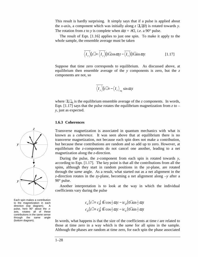
During the pulse, the z-component from each spin is rotated towards y,according to Eqn. [1.17]. The key point is that all the contributions from all thespins, although they start in random positions in the yz-plane, are rotatedthrough the same angle. As a result, what started out as a net alignment in thez-direction rotates in the zy-plane, becoming a net alignment along –y after a90° pulse.

Another interpretation is to look at the way in which the individualcoefficients vary during the pulse

( ) ( ) ( )( ) ( ) ( )

c t c t ic t

c t c t ic t

α α β

β β α

ω ω

ω ω

= −

= −

0 0

0 0

12 1

12 1

12 1

12 1

cos sin

cos sin

In words, what happens is that the size of the coefficients at time t are related tothose at time zero in a way which is the same for all spins in the sample.Although the phases are random at time zero, for each spin the phase associated

y

y

z

z

Each spin makes a contributionto the magnetization in eachdirection (top diagram). Apulse, here 90° about the x-axis, rotates all of thesecontributions in the same sensethrough the same angle(bottom diagram).

1–29

with cα at time zero is transferred to cβ, and vice versa. It is this correlation ofphases between the two coefficients which leads to an overall observable signalfrom the sample.

'HQVLW\PDWUL[

The approach used in the previous section is rather inconvenient for calculatingthe outcome of NMR experiments. In particular, the need for ensembleaveraging after the calculation has been completed is especially difficult. Itturns out that there is an alternative way of casting the Schrödinger equationwhich leads to a much more convenient framework for calculation – this isdensity matrix theory. This theory, can be further modified to give an operatorversion which is generally the most convenient for calculations in multiplepulse NMR.

First, the idea of matrix representations of operators needs to be introduced.

1.7.1 Matrix representations

An operator, Q, can be represented as a matrix in a particular basis set offunctions. A basis set is a complete set of wavefunctions which are adequatefor describing the system, for example in the case of a single spin the twofunctions |α⟩ and |β⟩ form a suitable basis. In larger spin systems, more basisfunctions are needed, for example the four product functions described insection 1.4.1.2 form such a basis for a two spin system.

The matrix form of Q is defined in this two-dimensional representation isdefined as

QQ Q

Q Q=

α α α ββ α β β

Each of the matrix elements, Qij, is calculated from an integral of the form⟨i|Q|j⟩, where |i⟩ and |j⟩ are two of the basis functions. The matrix element Qij

appears in the ith row and the jth column.

1.7.1.1 One spin

Particularly important are the matrix representations of the angular momentumoperators. For example, Iz:

Iz|α⟩ = (1/2) |α⟩

Iz|β⟩ = –(1/2) |β⟩

⟨α|β⟩ = ⟨β|α⟩ = 0

⟨α|α⟩ = ⟨β|β⟩ = 1

1–30

II I

I Izz z

z z

=

=−−

=−

α α α ββ α β β

α α α ββ α β β

12

12

12

12

12

12

0

0

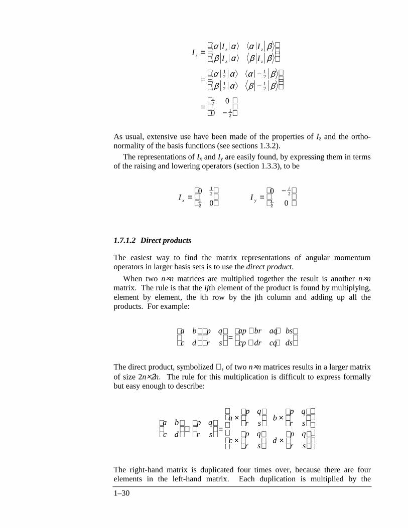
As usual, extensive use have been made of the properties of Iz and the ortho-normality of the basis functions (see sections 1.3.2).

The representations of Ix and Iy are easily found, by expressing them in termsof the raising and lowering operators (section 1.3.3), to be

I Ix y

i

i=

=

−

0

0

0

0

12

12

2

2

1.7.1.2 Direct products

The easiest way to find the matrix representations of angular momentumoperators in larger basis sets is to use the direct product.

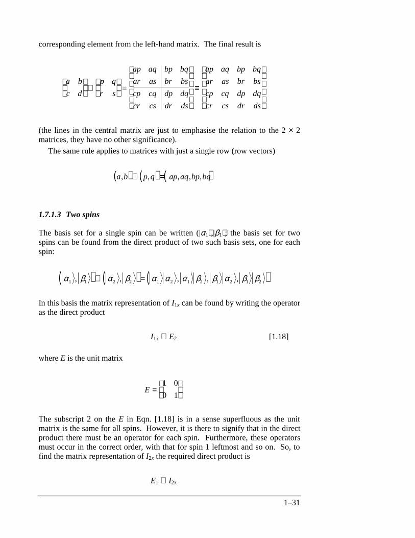
When two n×n matrices are multiplied together the result is another n×nmatrix. The rule is that the ijth element of the product is found by multiplying,element by element, the ith row by the jth column and adding up all theproducts. For example:

a b

c d

p q

r s

ap br aq bs

cp dr cq ds

=

+ ++ +

The direct product, symbolized ⊗, of two n×n matrices results in a larger matrixof size 2n×2n. The rule for this multiplication is difficult to express formallybut easy enough to describe:

a b

c d

p q

r s

ap q

r sb

p q

r s

cp q

r sd

p q

r s

⊗

=

×

×

×

×

The right-hand matrix is duplicated four times over, because there are fourelements in the left-hand matrix. Each duplication is multiplied by the

1–31

corresponding element from the left-hand matrix. The final result is

a b

c d

p q

r s

ap aq bp bq

ar as br bs

cp cq dp dq

cr cs dr ds

ap aq bp bq

ar as br bs

cp cq dp dq

cr cs dr ds

⊗

=

≡

(the lines in the central matrix are just to emphasise the relation to the 2 × 2matrices, they have no other significance).

The same rule applies to matrices with just a single row (row vectors)

( ) ( ) ( )a b p q ap aq bp bq, , , , ,⊗ =

1.7.1.3 Two spins

The basis set for a single spin can be written (|α1⟩,|β1⟩; the basis set for twospins can be found from the direct product of two such basis sets, one for eachspin:

( ) ( ) ( )α β α β α α α β β α β β1 1 2 2 1 2 1 2 1 2 1 2, , , , ,⊗ =

In this basis the matrix representation of I1x can be found by writing the operatoras the direct product

I1x ⊗ E2 [1.18]

where E is the unit matrix

E =

1 0

0 1

The subscript 2 on the E in Eqn. [1.18] is in a sense superfluous as the unitmatrix is the same for all spins. However, it is there to signify that in the directproduct there must be an operator for each spin. Furthermore, these operatorsmust occur in the correct order, with that for spin 1 leftmost and so on. So, tofind the matrix representation of I2x the required direct product is

E1 ⊗ I2x

1–32

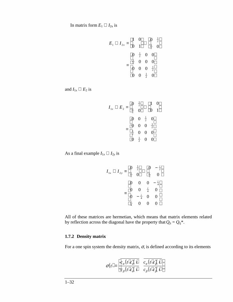
In matrix form E1 ⊗ I2x is

E I x1 2

12

12

12

12

12

12

1 0

0 1

0

0

0 0 0

0 0 0

0 0 0

0 0 0

⊗ =

⊗

=

and I1x ⊗ E2 is

I Ex1 2

12

12

12

12

12

12

0

0

1 0

0 1

0 0 0

0 0 0

0 0 0

0 0 0

⊗ =

⊗

=

As a final example I1x ⊗ I2y is

I Ix y

i

i

i

i

i

i

1 2

12

12

2

2

4

4

4

4

0

0

0

0

0 0 0

0 0 0

0 0 0

0 0 0

⊗ =

⊗

−

=

−

−

All of these matrices are hermetian, which means that matrix elements relatedby reflection across the diagonal have the property that Qji = Qij*.

1.7.2 Density matrix

For a one spin system the density matrix, σ, is defined according to its elements

( )( ) ( ) ( ) ( )( ) ( ) ( ) ( )

σ α α α β

β α β β

tc t c t c t c t

c t c t c t c t=

* *

* *

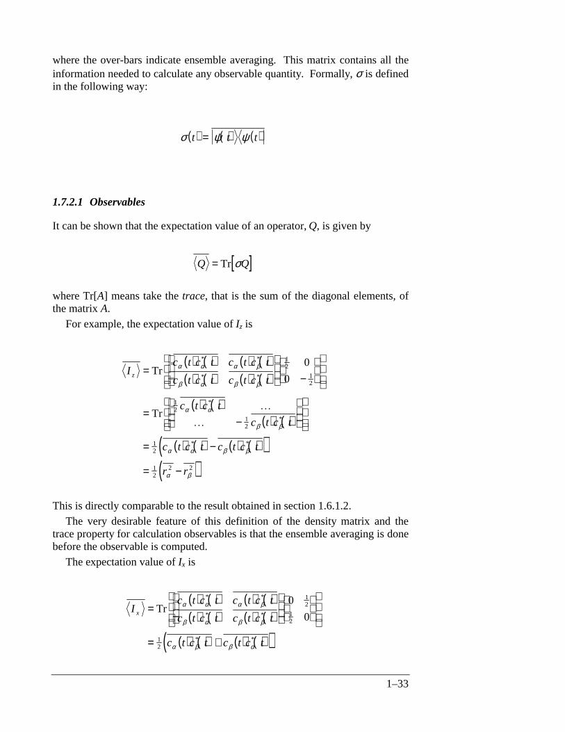
1–33

where the over-bars indicate ensemble averaging. This matrix contains all theinformation needed to calculate any observable quantity. Formally, σ is definedin the following way:

( ) ( ) ( )σ ψ ψt t t=

1.7.2.1 Observables

It can be shown that the expectation value of an operator, Q, is given by

[ ]Q Q= Tr σ

where Tr[A] means take the trace, that is the sum of the diagonal elements, ofthe matrix A.

For example, the expectation value of Iz is

( ) ( ) ( ) ( )( ) ( ) ( ) ( )

( ) ( )( ) ( )

( ) ( ) ( ) ( )( )( )

Ic t c t c t c t

c t c t c t c t

c t c t

c t c t

c t c t c t c t

r r

z =

−

=−

= −

= −

Tr

Tr

α α α β

β α β β

α α

β β

α α β β

α β

* *

* *

*

*

* *

12

12

12

12

12

12

2 2

0

0

K

K

This is directly comparable to the result obtained in section 1.6.1.2.The very desirable feature of this definition of the density matrix and the

trace property for calculation observables is that the ensemble averaging is donebefore the observable is computed.

The expectation value of Ix is

( ) ( ) ( ) ( )( ) ( ) ( ) ( )

( ) ( ) ( ) ( )( )

Ic t c t c t c t

c t c t c t c t

c t c t c t c t

x =

= +

Tr α α α β

β α β β

α β β α

* *

* *

* *

0

0

12

12

12

1–34

Again, this is directly comparable to the result obtained in section 1.6.1.2The off diagonal elements of the density matrix can contribute to transverse

magnetization, whereas the diagonal elements only contribute to longitudinal

magnetization. In general, a non-zero off-diagonal element ( ) ( )c t c ti j* indicates

a coherence involving levels i and j, whereas a diagonal element, ( ) ( )c t c ti i* ,

indicates the population of level i.From now on the ensemble averaging and time dependence will be taken as

implicit and so the elements of the density matrix will be written simply c ci j*

unless there is any ambiguity.

1.7.2.2 Equilibrium

As described in section 1.6.1.2, at equilibrium the phases of the super-position

states are random and as a result the ensemble averages ( ) ( )c t c tα β* and

( ) ( )c t c tβ α* are zero. This is easily seen by writing then in the r/φ format

( ) ( )c c r i r iα β α α β βφ φ* exp exp= −

= 0 at equilibrium

However, the diagonal elements do not average to zero but rather correspond tothe populations, Pi, of the levels, as was described in section 1.6.1.2

( ) ( )c c r i r i

r

P

α α α α α α

α

α

φ φ* exp exp= −

==

2

The equilibrium density matrix for one spin is thus

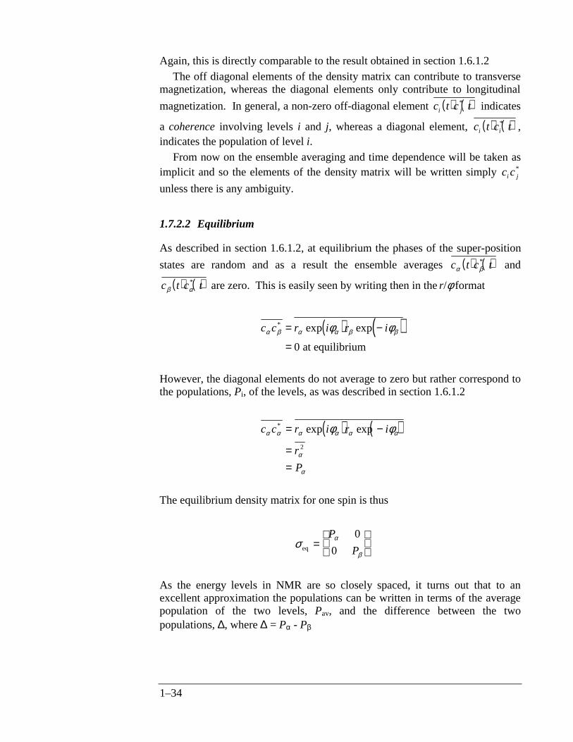
σ α

βeq =

P

P

0

0

As the energy levels in NMR are so closely spaced, it turns out that to anexcellent approximation the populations can be written in terms of the averagepopulation of the two levels, Pav, and the difference between the twopopulations, ∆, where ∆ = Pα - Pβ

1–35

σeqav

av

=+

−

P

P

12

12

0

0

∆∆

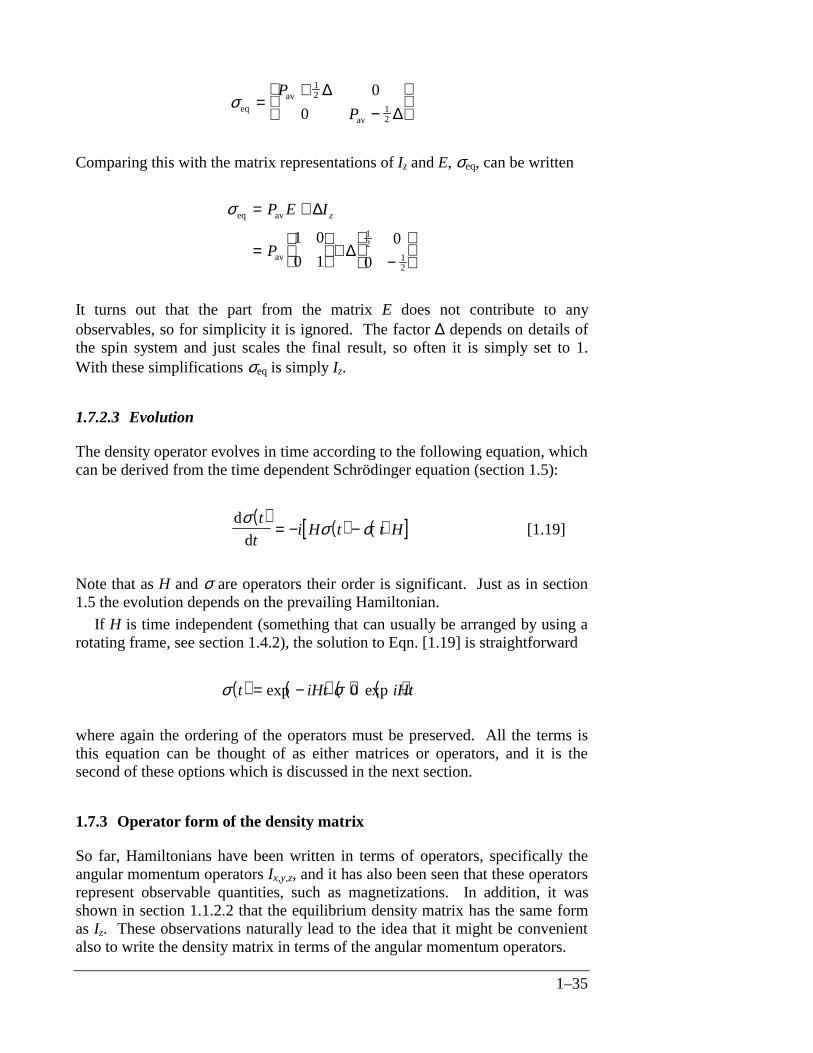
Comparing this with the matrix representations of Iz and E, σeq, can be written

σeq av

av

= +

=

+

−

P E I

P

z∆

∆1 0

0 1

0

0

12

12

It turns out that the part from the matrix E does not contribute to anyobservables, so for simplicity it is ignored. The factor ∆ depends on details ofthe spin system and just scales the final result, so often it is simply set to 1.With these simplifications σeq is simply Iz.

1.7.2.3 Evolution

The density operator evolves in time according to the following equation, whichcan be derived from the time dependent Schrödinger equation (section 1.5):

( ) ( ) ( )[ ]d

d

σσ σ

t

ti H t t H= − − [1.19]

Note that as H and σ are operators their order is significant. Just as in section1.5 the evolution depends on the prevailing Hamiltonian.

If H is time independent (something that can usually be arranged by using arotating frame, see section 1.4.2), the solution to Eqn. [1.19] is straightforward

( ) ( ) ( ) ( )σ σt iHt iHt= −exp exp0

where again the ordering of the operators must be preserved. All the terms isthis equation can be thought of as either matrices or operators, and it is thesecond of these options which is discussed in the next section.

1.7.3 Operator form of the density matrix

So far, Hamiltonians have been written in terms of operators, specifically theangular momentum operators Ix,y,z, and it has also been seen that these operatorsrepresent observable quantities, such as magnetizations. In addition, it wasshown in section 1.1.2.2 that the equilibrium density matrix has the same formas Iz. These observations naturally lead to the idea that it might be convenientalso to write the density matrix in terms of the angular momentum operators.

1–36

Specifically, the idea is to expand the density matrix as a combination of theoperators:

σ(t) = a(t)Iz + b(t)Iy + c(t)Iz

where a, b and c are coefficients which depend on time.

1.7.3.1 Observables

From this form of the density matrix, the expectation value of, for example, Ix

can be computed in the usual way (section 1.7.2.1).

[ ]( )[ ]

[ ] [ ] [ ]

I I

aI bI cI I

aI I bI I cI I

x x

x y z x

x x y x z x

=

= + +

= + +

Tr

Tr

Tr Tr Tr

σ

where to get to the last line the property that the trace of a sum of matrices isequal to the sum of the traces of the matrices has been used.

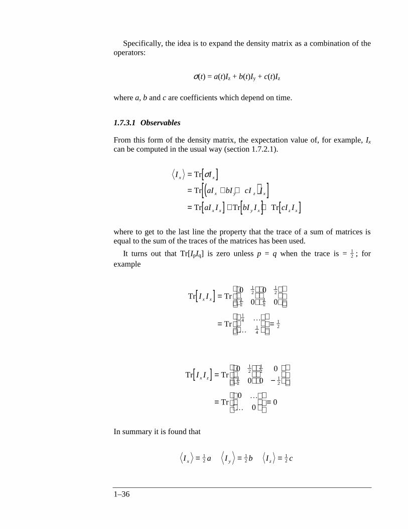
It turns out that Tr[IpIq] is zero unless p = q when the trace is = 12 ; for

example

[ ]Tr Tr

Tr

I Ix x =

=

=

0

0

0

0

12

12

12

12

14

14

12

K

K

[ ]Tr Tr

Tr

I Ix z =

−

=

=

0

0

0

0

0

00

12

12

12

12

K

K

In summary it is found that

I a I b I cx y z= = =12

12

12

1–37

This is a very convenient result. By expressing the density operator in the formσ(t) = a(t)Iz + b(t)Iy + c(t)Iz the x-, y- and z-magnetizations can be deduced justby inspection as being proportional to a(t), b(t), and c(t) respectively (the factorof one half is not important). This approach is further developed in the lecture 2where the product operator method is introduced.

1.7.3.2 Evolution

The evolution of the density matrix follows the equation

( ) ( ) ( ) ( )σ σt iHt iHt= −exp exp0

Often the Hamiltonian will be a sum of terms, for example, in the case of freeprecession for two spins H = Ω1I1z + Ω2I2z. The exponential of the sum of twooperators can be expressed as a product of two exponentials provided theoperators commute

( ) ( ) ( )exp exp expA B A B A B+ = provided and commute

Commuting operators are ones whose effect is unaltered by changing theirorder: i.e. ABψ = BAψ; not all operators commute with one another.

Luckily, operators for different spins do commute so, for the free precessionHamiltonian

( ) [ ]( )( ) ( )

exp exp

exp exp

− = − +

= − −

iHt i I I t

i I t i I t

z z

z z

Ω Ω

Ω Ω1 1 2 2

1 1 2 2

The evolution of the density matrix can then be written

( ) ( ) ( ) ( ) ( ) ( )σ σt i I t i I t i I t i I tz z z z= − −exp exp exp expΩ Ω Ω Ω1 1 2 2 1 1 2 20

The operators for the evolution due to offsets and couplings also commute withone another.

For commuting operators the order is immaterial. This applies also to theirexponentials, e.g. exp(A) B = B exp(A). This property is used in the following

( ) ( ) ( ) ( )( )( )

exp exp exp exp

exp

exp

− = −

= − +

= =

i I t I i I t i I t i I t I

i I t i I t I

I I

z x z z z x

z z x

x x

Ω Ω Ω Ω

Ω Ω1 1 2 1 1 1 1 1 1 2

1 1 1 1 2

2 20

1–38

In words this says that the offset of spin 1 causes no evolution of transversemagnetization of spin 2.

These various properties will be used extensively in lecture 2.