09 Discrete Cosine Transform

388

JJIIJI

Back

Close

Moving into the Frequency Domain

Frequency domains can be obtained through thetransformation from one (Time or Spatial) domain to the other(Frequency) via

• Discrete Cosine Transform (DCT)— Heart of JPEG andMPEG Video, (alt.) MPEG Audio. (New)

• Fourier Transform (FT) — MPEG Audio (See Tutorial 2 —RecallFrom CM0268 and )

Note: We mention some image (and video) examples in this sectionwith DCT (in particular) but also the FT is commonly applied to filtermultimedia data.

389

JJIIJI

Back

Close

Recap: What do frequencies mean in animage?• Large values at high frequency components then the data

is changing rapidly on a short distance scale.e.g. a page of text

• Large low frequency components then the large scale featuresof the picture are more important.e.g. a single fairly simple object which occupies most of theimage.

390

JJIIJI

Back

Close

The Road to CompressionHow do we achieve compression?

• Low pass filter — ignore high frequency noise components

– Only store lower frequency components

• High Pass Filter — Spot Gradual Changes

– If changes to low Eye does not respond so ignore?

391

JJIIJI

Back

Close

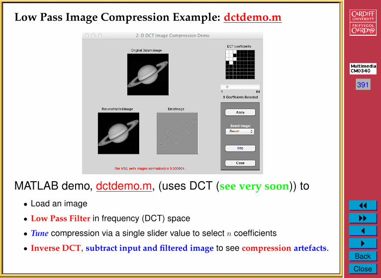
Low Pass Image Compression Example: dctdemo.m

MATLAB demo, dctdemo.m, (uses DCT (see very soon)) to• Load an image

• Low Pass Filter in frequency (DCT) space

• Tune compression via a single slider value to select n coefficients

• Inverse DCT, subtract input and filtered image to see compression artefacts.

392

JJIIJI

Back

Close

Recap: Fourier Transform

The tool which converts a spatial (real space) description ofaudio/image data into one in terms of its frequency componentsis called the Fourier transform

The new version is usually referred to as the Fourier spacedescription of the data.We then essentially process the data:

• E.g. for filtering basically this means attenuating or settingcertain frequencies to zero

We then need to convert data back to real audio/imagery to usein our applications.

The corresponding inverse transformation which turns a Fourierspace description back into a real space one is called theinverse Fourier transform.

393

JJIIJI

Back

Close

The Discrete Cosine Transform (DCT)Relationship between DCT and FFT

DCT (Discrete Cosine Transform) is actually a cut-down versionof the Fourier Transform or the Fast Fourier Transform (FFT):

• Only the real part of FFT

• Computationally simpler than FFT

• DCT — Effective for Multimedia Compression

• DCT MUCH more commonly used (than FFT) in MultimediaImage/Video Compression — more later

• Cheap MPEG Audio Variant — more later

394

JJIIJI

Back

Close

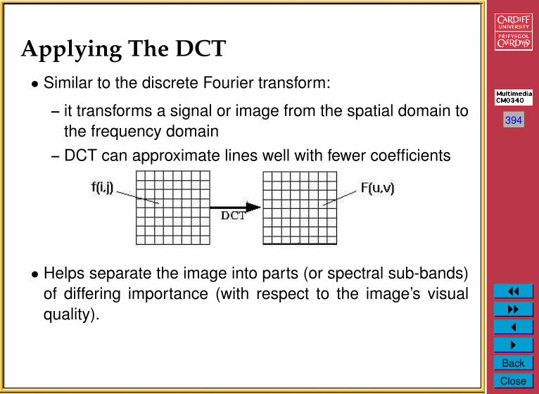
Applying The DCT• Similar to the discrete Fourier transform:

– it transforms a signal or image from the spatial domain tothe frequency domain

– DCT can approximate lines well with fewer coefficients

• Helps separate the image into parts (or spectral sub-bands)of differing importance (with respect to the image’s visualquality).

395

JJIIJI

Back

Close

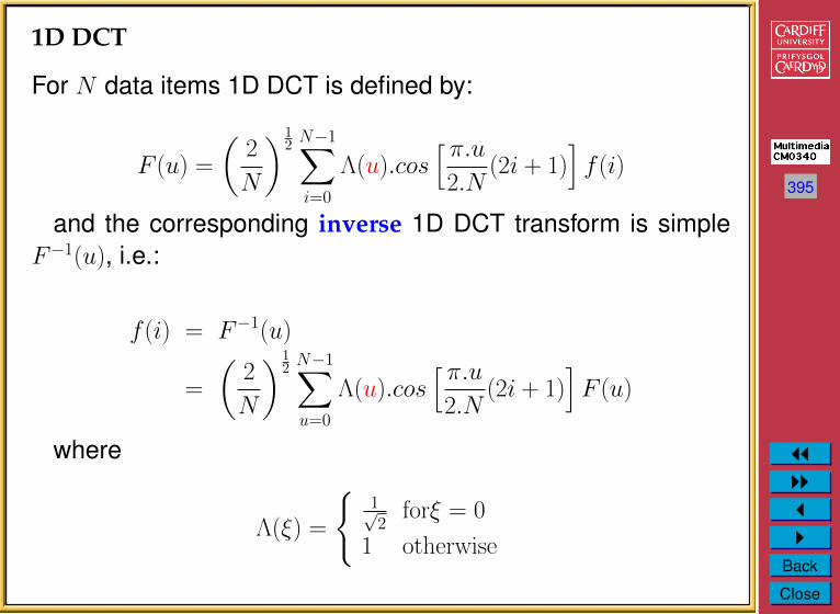
1D DCT

For N data items 1D DCT is defined by:

F (u) =

(2

N

)12N−1∑i=0

Λ(u).cos[ π.u

2.N(2i + 1)

]f (i)

and the corresponding inverse 1D DCT transform is simpleF−1(u), i.e.:

f (i) = F−1(u)

=

(2

N

)12N−1∑u=0

Λ(u).cos[ π.u

2.N(2i + 1)

]F (u)

where

Λ(ξ) =

{1√2

forξ = 0

1 otherwise

396

JJIIJI

Back

Close

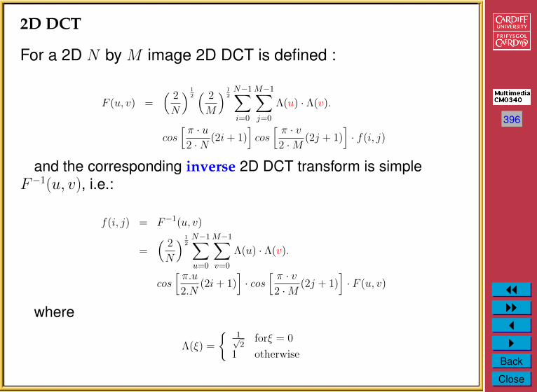
2D DCT

For a 2D N by M image 2D DCT is defined :

F (u, v) =(

2

N

) 12(

2

M

) 12N−1∑i=0

M−1∑j=0

Λ(u) · Λ(v).

cos[π · u2 ·N

(2i+ 1)]cos[π · v2 ·M

(2j + 1)]· f(i, j)

and the corresponding inverse 2D DCT transform is simpleF−1(u, v), i.e.:

f(i, j) = F−1(u, v)

=(

2

N

) 12N−1∑u=0

M−1∑v=0

Λ(u) · Λ(v).

cos[π.u

2.N(2i+ 1)

]· cos

[π · v2 ·M

(2j + 1)]· F (u, v)

where

Λ(ξ) =

{1√2

forξ = 0

1 otherwise

397

JJIIJI

Back

Close

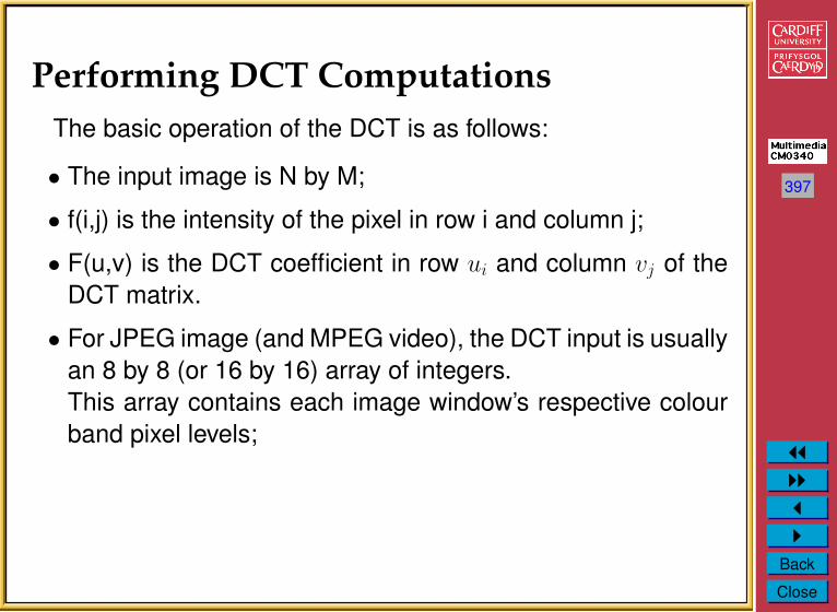
Performing DCT ComputationsThe basic operation of the DCT is as follows:

• The input image is N by M;

• f(i,j) is the intensity of the pixel in row i and column j;

• F(u,v) is the DCT coefficient in row ui and column vj of theDCT matrix.

• For JPEG image (and MPEG video), the DCT input is usuallyan 8 by 8 (or 16 by 16) array of integers.This array contains each image window’s respective colourband pixel levels;

398

JJIIJI

Back

Close

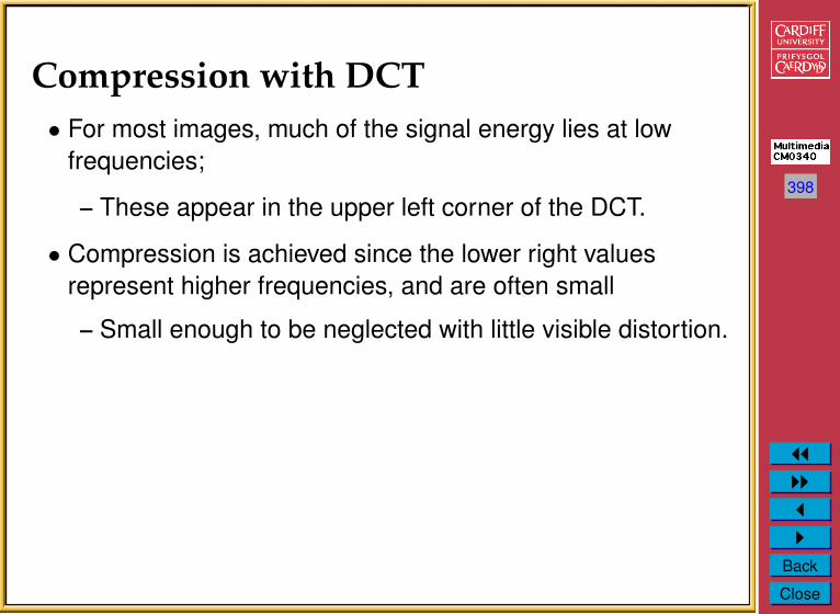
Compression with DCT• For most images, much of the signal energy lies at low

frequencies;

– These appear in the upper left corner of the DCT.

• Compression is achieved since the lower right valuesrepresent higher frequencies, and are often small

– Small enough to be neglected with little visible distortion.

399

JJIIJI

Back

Close

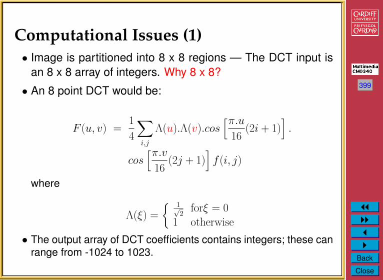
Computational Issues (1)• Image is partitioned into 8 x 8 regions — The DCT input is

an 8 x 8 array of integers. Why 8 x 8?

• An 8 point DCT would be:

F (u, v) =1

4

∑i,j

Λ(u).Λ(v).cos[π.u

16(2i + 1)

].

cos[π.v

16(2j + 1)

]f (i, j)

where

Λ(ξ) =

{ 1√2

forξ = 01 otherwise

• The output array of DCT coefficients contains integers; these canrange from -1024 to 1023.

400

JJIIJI

Back

Close

Computational Issues (2)

• Computationally easier to implement and more efficient toregard the DCT as a set of basis functions

– Given a known input array size (8 x 8) can be precomputedand stored.

– Computing values for a convolution mask (8 x 8 window)that get applied∗ Sum values x pixel the window overlap with image apply

window across all rows/columns of image– The values as simply calculated from DCT formula.

401

JJIIJI

Back

Close

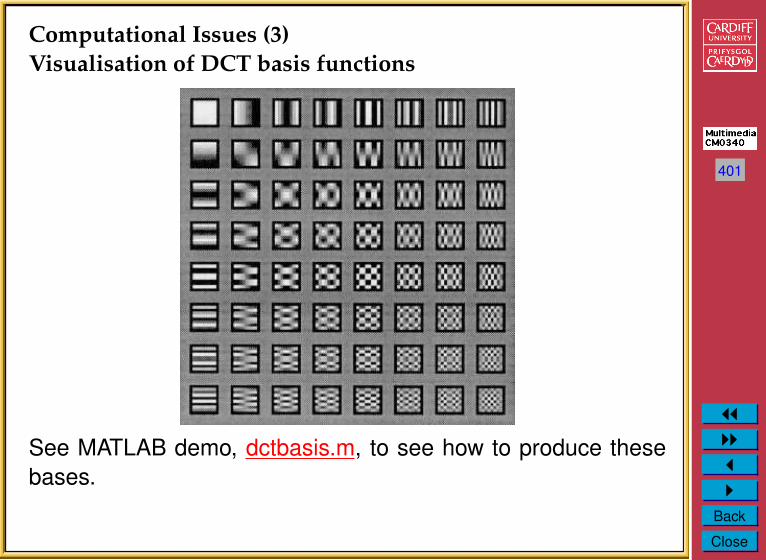
Computational Issues (3)Visualisation of DCT basis functions

See MATLAB demo, dctbasis.m, to see how to produce thesebases.

402

JJIIJI

Back

Close

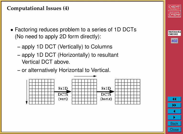
Computational Issues (4)

• Factoring reduces problem to a series of 1D DCTs(No need to apply 2D form directly):

– apply 1D DCT (Vertically) to Columns– apply 1D DCT (Horizontally) to resultant

Vertical DCT above.– or alternatively Horizontal to Vertical.

403

JJIIJI

Back

Close

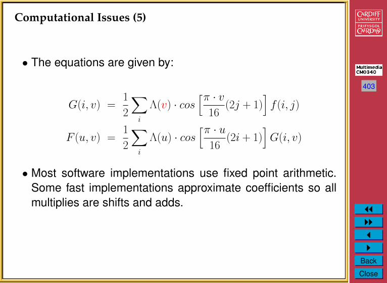
Computational Issues (5)

• The equations are given by:

G(i, v) =1

2

∑i

Λ(v) · cos[π · v

16(2j + 1)

]f (i, j)

F (u, v) =1

2

∑i

Λ(u) · cos[π · u

16(2i + 1)

]G(i, v)

• Most software implementations use fixed point arithmetic.Some fast implementations approximate coefficients so allmultiplies are shifts and adds.

404

JJIIJI

Back

Close

Filtering in the Frequency Domain: Somemore examples

FT and DCT methods pretty similar:

• DCT has less data overheads — no complex array part

• FT captures more frequency ’fidelity’ (e.g. Phase).

Low Pass Filter

Example: Frequencies above the Nyquist Limit,Noise:

• The idea with noise smoothing is to reduce various spuriouseffects of a local nature in the image, caused perhaps by

– noise in the acquisition system,

405

JJIIJI

Back

Close

– arising as a result of transmission of the data, for examplefrom a space probe utilising a low-power transmitter.

406

JJIIJI

Back

Close

Recap: Frequency Space Smoothing Methods

Noise = High Frequencies:

• In audio data many spurious peaks in over a short timescale.

• In an image means there are many rapid transitions (over ashort distance) in intensity from high to low and back againor vice versa, as faulty pixels are encountered.

• Not all high frequency data noise though!

Therefore noise will contribute heavily to the high frequencycomponents of the image when it is considered in Fourier space.

Thus if we reduce the high frequency components — Low-PassFilter, we should reduce the amount of noise in the data.

407

JJIIJI

Back

Close

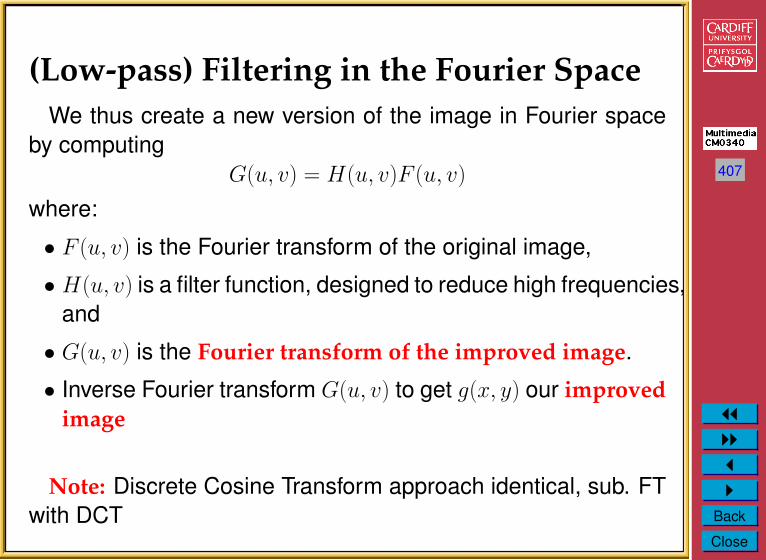
(Low-pass) Filtering in the Fourier SpaceWe thus create a new version of the image in Fourier space

by computingG(u, v) = H(u, v)F (u, v)

where:

• F (u, v) is the Fourier transform of the original image,

• H(u, v) is a filter function, designed to reduce high frequencies,and

• G(u, v) is the Fourier transform of the improved image.

• Inverse Fourier transform G(u, v) to get g(x, y) our improvedimage

Note: Discrete Cosine Transform approach identical, sub. FTwith DCT

408

JJIIJI

Back

Close

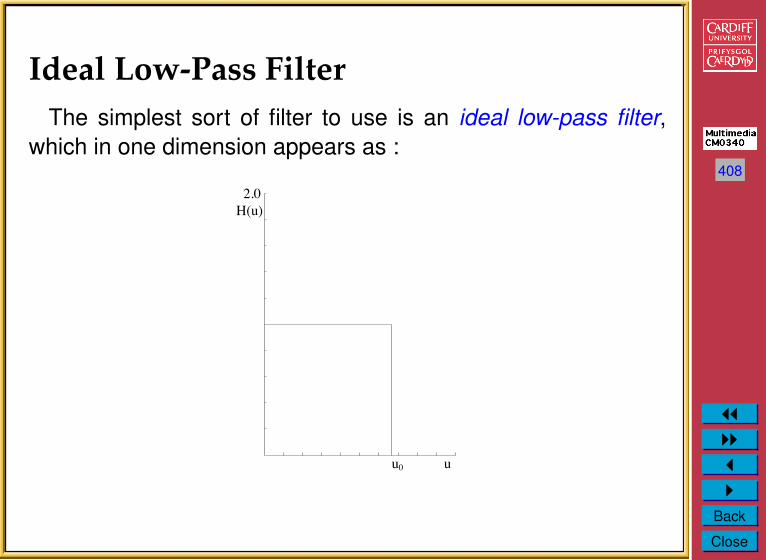
Ideal Low-Pass FilterThe simplest sort of filter to use is an ideal low-pass filter,

which in one dimension appears as :

uu0

2.0

H(u)

409

JJIIJI

Back

Close

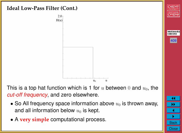
Ideal Low-Pass Filter (Cont.)

uu0

2.0

H(u)

This is a top hat function which is 1 for u between 0 and u0, thecut-off frequency, and zero elsewhere.

• So All frequency space information above u0 is thrown away,and all information below u0 is kept.

• A very simple computational process.

410

JJIIJI

Back

Close

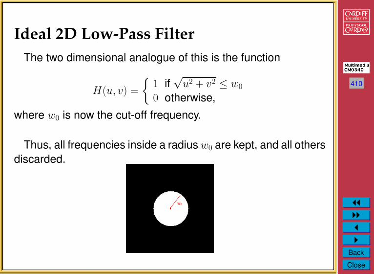
Ideal 2D Low-Pass FilterThe two dimensional analogue of this is the function

H(u, v) =

{1 if√u2 + v2 ≤ w0

0 otherwise,where w0 is now the cut-off frequency.

Thus, all frequencies inside a radius w0 are kept, and all othersdiscarded.

w0

411

JJIIJI

Back

Close

Not So Ideal Low-Pass Filter?

The problem with this filter is that as well as the noise:

• In audio: plenty of other high frequency content

• In Images: edges (places of rapid transition from light todark) also significantly contribute to the high frequencycomponents.

Thus an ideal low-pass filter will tend to blur the data:

• High audio frequencies become muffled

• Edges in images become blurred.

The lower the cut-off frequency is made, the more pronouncedthis effect becomes in useful data content

412

JJIIJI

Back

Close

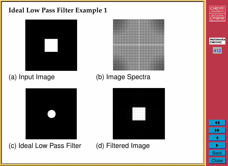
Ideal Low Pass Filter Example 1

(a) Input Image

(c) Ideal Low Pass Filter

(b) Image Spectra

(d) Filtered Image

413

JJIIJI

Back

Close

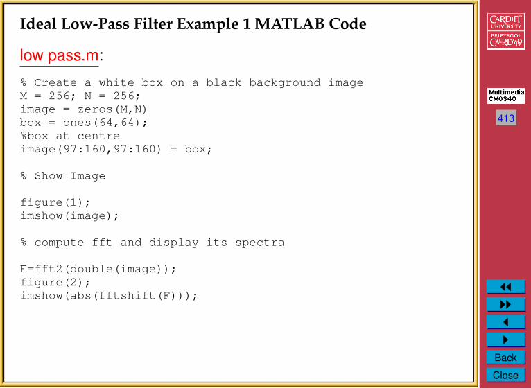
Ideal Low-Pass Filter Example 1 MATLAB Code

low pass.m:

% Create a white box on a black background imageM = 256; N = 256;image = zeros(M,N)box = ones(64,64);%box at centreimage(97:160,97:160) = box;

% Show Image

figure(1);imshow(image);

% compute fft and display its spectra

F=fft2(double(image));figure(2);imshow(abs(fftshift(F)));

414

JJIIJI

Back

Close

Ideal Low-Pass Filter Example 1 MATLAB Code (Cont.)%compute Ideal Low Pass Filteru0 = 20; % set cut off frequency

u=0:(M-1);v=0:(N-1);idx=find(u>M/2);u(idx)=u(idx)-M;idy=find(v>N/2);v(idy)=v(idy)-N;[V,U]=meshgrid(v,u);D=sqrt(U.ˆ2+V.ˆ2);H=double(D<=u0);

% displayfigure(3);imshow(fftshift(H));

% Apply filter and do inverse FFTG=H.*F;g=real(ifft2(double(G)));

% Show Resultfigure(4);imshow(g);

415

JJIIJI

Back

Close

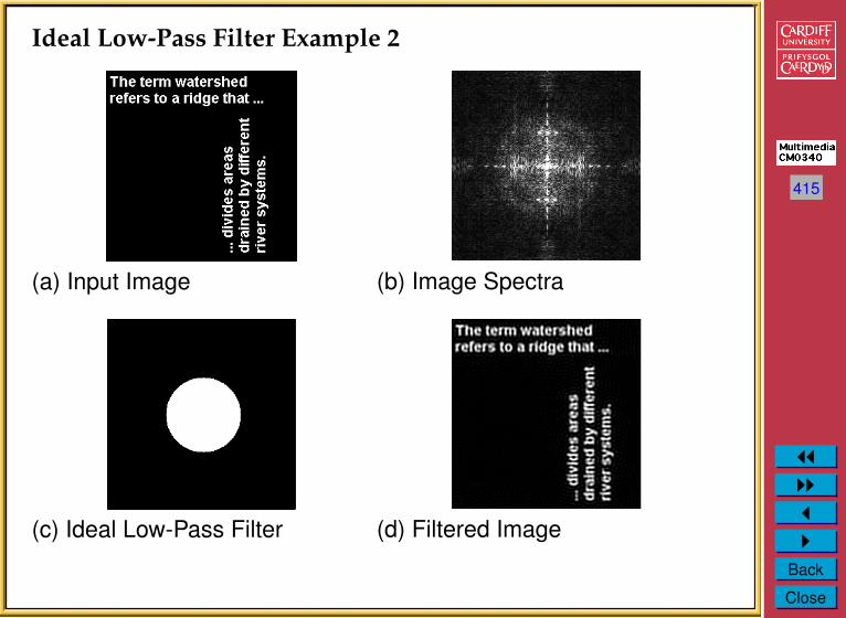
Ideal Low-Pass Filter Example 2

(a) Input Image

(c) Ideal Low-Pass Filter

(b) Image Spectra

(d) Filtered Image

416

JJIIJI

Back

Close

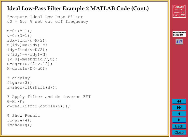
Ideal Low-Pass Filter Example 2 MATLAB Code

lowpass2.m:

% read in MATLAB demo text imageimage = imread(’text.png’);[M N] = size(image)

% Show Image

figure(1);imshow(image);

% compute fft and display its spectra

F=fft2(double(image));figure(2);imshow(abs(fftshift(F))/256);

417

JJIIJI

Back

Close

Ideal Low-Pass Filter Example 2 MATLAB Code (Cont.)%compute Ideal Low Pass Filteru0 = 50; % set cut off frequency

u=0:(M-1);v=0:(N-1);idx=find(u>M/2);u(idx)=u(idx)-M;idy=find(v>N/2);v(idy)=v(idy)-N;[V,U]=meshgrid(v,u);D=sqrt(U.ˆ2+V.ˆ2);H=double(D<=u0);

% displayfigure(3);imshow(fftshift(H));

% Apply filter and do inverse FFTG=H.*F;g=real(ifft2(double(G)));

% Show Resultfigure(4);imshow(g);

418

JJIIJI

Back

Close

Low-Pass Butterworth Filter

Another filter sometimes used is the Butterworth low pass filter.

In the 2D case, H(u, v) takes the form

H(u, v) =1

1 + [(u2 + v2)/w20]n ,

where n is called the order of the filter.

419

JJIIJI

Back

Close

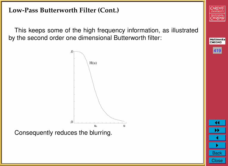
Low-Pass Butterworth Filter (Cont.)

This keeps some of the high frequency information, as illustratedby the second order one dimensional Butterworth filter:

u0 u.0

.0

H(u)

Consequently reduces the blurring.

420

JJIIJI

Back

Close

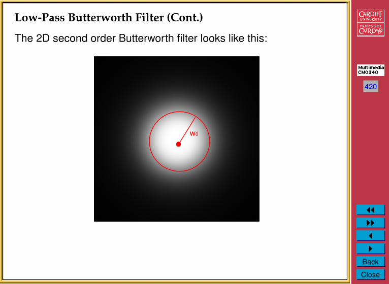
Low-Pass Butterworth Filter (Cont.)

The 2D second order Butterworth filter looks like this:

w0

421

JJIIJI

Back

Close

Butterworth Low Pass Filter Example 1

(a) Input Image

(c) Butterworth Low-Pass Filter

(b) Image Spectra

(d) Filtered Image

422

JJIIJI

Back

Close

Butterworth Low-Pass Filter Example 1 (Cont.)

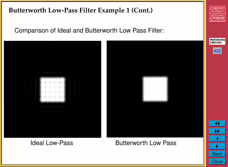
Comparison of Ideal and Butterworth Low Pass Filter:

Ideal Low-Pass Butterworth Low Pass

423

JJIIJI

Back

Close

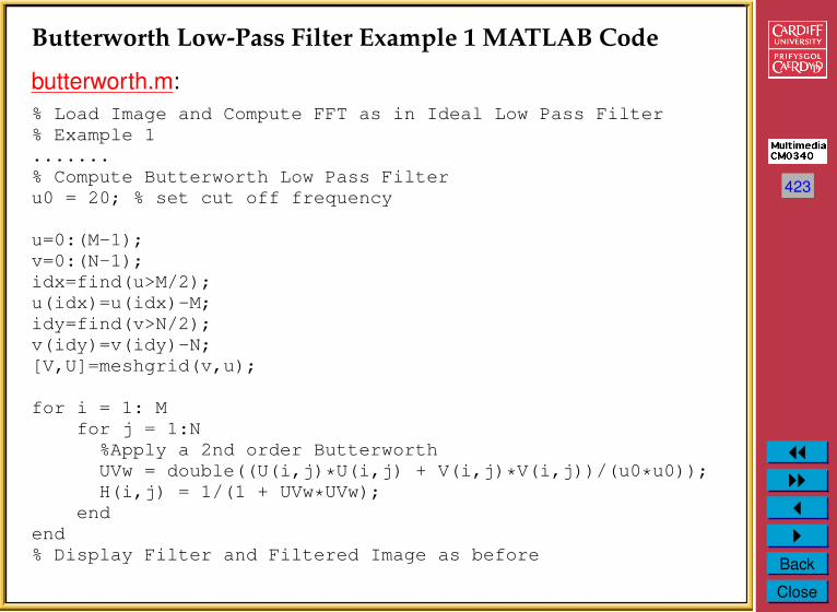
Butterworth Low-Pass Filter Example 1 MATLAB Code

butterworth.m:% Load Image and Compute FFT as in Ideal Low Pass Filter% Example 1.......% Compute Butterworth Low Pass Filteru0 = 20; % set cut off frequency

u=0:(M-1);v=0:(N-1);idx=find(u>M/2);u(idx)=u(idx)-M;idy=find(v>N/2);v(idy)=v(idy)-N;[V,U]=meshgrid(v,u);

for i = 1: Mfor j = 1:N%Apply a 2nd order ButterworthUVw = double((U(i,j)*U(i,j) + V(i,j)*V(i,j))/(u0*u0));H(i,j) = 1/(1 + UVw*UVw);

endend% Display Filter and Filtered Image as before

424

JJIIJI

Back

Close

Butterworth Low-Pass Butterworth Filter Example 2

(a) Input Image

(c) Butterworth Low-Pass Filter

(b) Image Spectra

(d) Filtered Image

425

JJIIJI

Back

Close

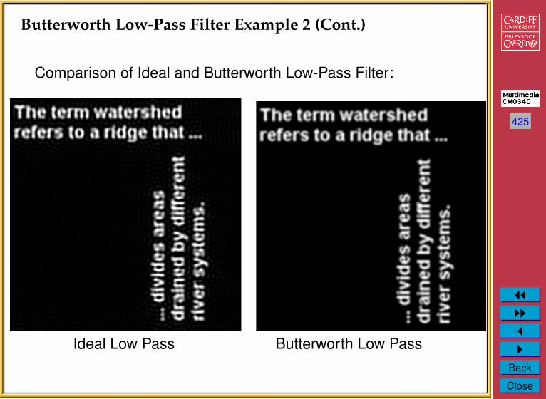
Butterworth Low-Pass Filter Example 2 (Cont.)

Comparison of Ideal and Butterworth Low-Pass Filter:

Ideal Low Pass Butterworth Low Pass

426

JJIIJI

Back

Close

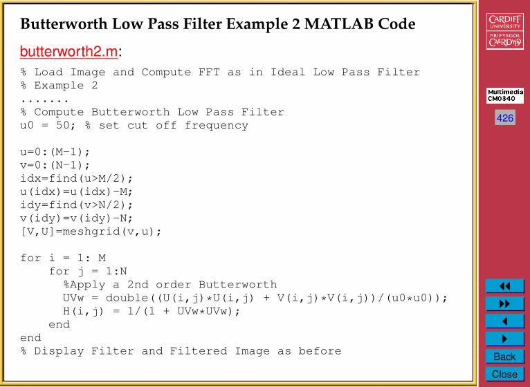
Butterworth Low Pass Filter Example 2 MATLAB Code

butterworth2.m:% Load Image and Compute FFT as in Ideal Low Pass Filter% Example 2.......% Compute Butterworth Low Pass Filteru0 = 50; % set cut off frequency

u=0:(M-1);v=0:(N-1);idx=find(u>M/2);u(idx)=u(idx)-M;idy=find(v>N/2);v(idy)=v(idy)-N;[V,U]=meshgrid(v,u);

for i = 1: Mfor j = 1:N%Apply a 2nd order ButterworthUVw = double((U(i,j)*U(i,j) + V(i,j)*V(i,j))/(u0*u0));H(i,j) = 1/(1 + UVw*UVw);

endend% Display Filter and Filtered Image as before

427

JJIIJI

Back

Close

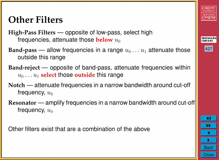
Other FiltersHigh-Pass Filters — opposite of low-pass, select high

frequencies, attenuate those below u0

Band-pass — allow frequencies in a range u0 . . . u1 attenuate thoseoutside this range

Band-reject — opposite of band-pass, attenuate frequencies withinu0 . . . u1 select those outside this range

Notch — attenuate frequencies in a narrow bandwidth around cut-offfrequency, u0

Resonator — amplify frequencies in a narrow bandwidth around cut-offfrequency, u0

Other filters exist that are a combination of the above

428

JJIIJI

Back

Close

ConvolutionSeveral important audio and optical effects can be described in

terms of convolutions.

• In fact the above Fourier filtering is applying convolutions of lowpass filter where the equations are Fourier Transforms of realspace equivalents.

• deblurring — high pass filtering

• reverb — see CM0268.

429

JJIIJI

Back

Close

1D Convolution

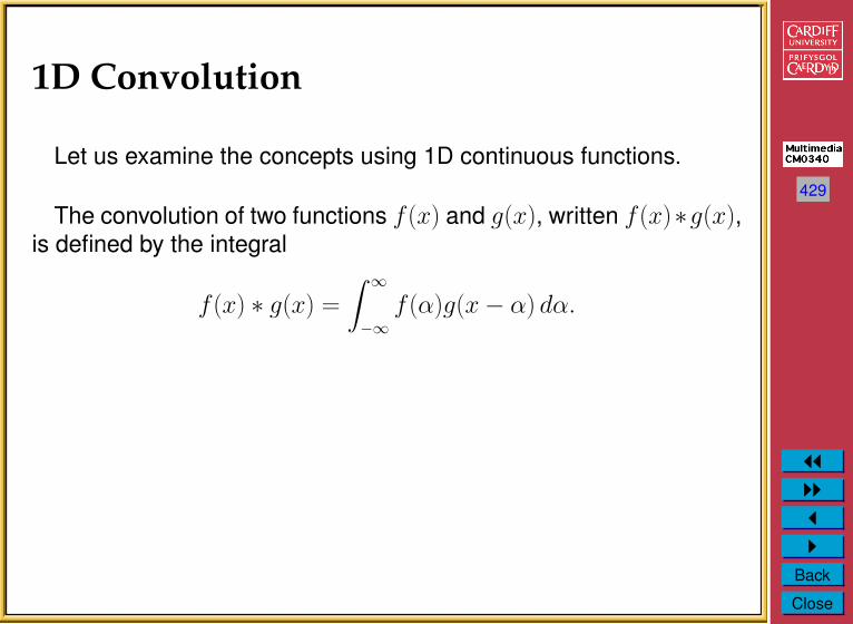
Let us examine the concepts using 1D continuous functions.

The convolution of two functions f (x) and g(x), written f (x)∗g(x),is defined by the integral

f (x) ∗ g(x) =

∫ ∞−∞

f (α)g(x− α) dα.

430

JJIIJI

Back

Close

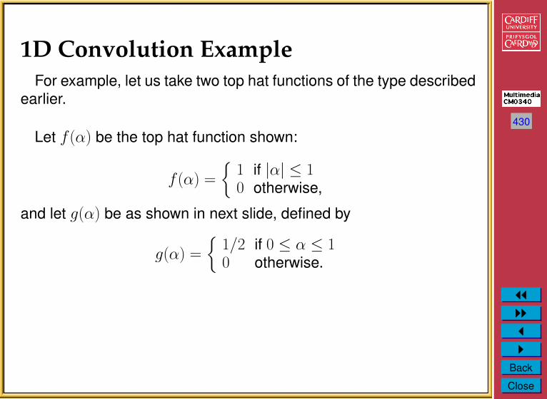
1D Convolution ExampleFor example, let us take two top hat functions of the type described

earlier.

Let f (α) be the top hat function shown:

f (α) =

{1 if |α| ≤ 10 otherwise,

and let g(α) be as shown in next slide, defined by

g(α) =

{1/2 if 0 ≤ α ≤ 10 otherwise.

431

JJIIJI

Back

Close

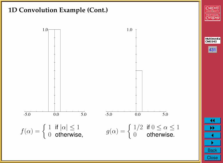
1D Convolution Example (Cont.)

-5.0 5.00.0

1.0

-5.0 5.00.0

1.0

f (α) =

{1 if |α| ≤ 10 otherwise, g(α) =

{1/2 if 0 ≤ α ≤ 10 otherwise.

432

JJIIJI

Back

Close

1D Convolution Example (Cont.)

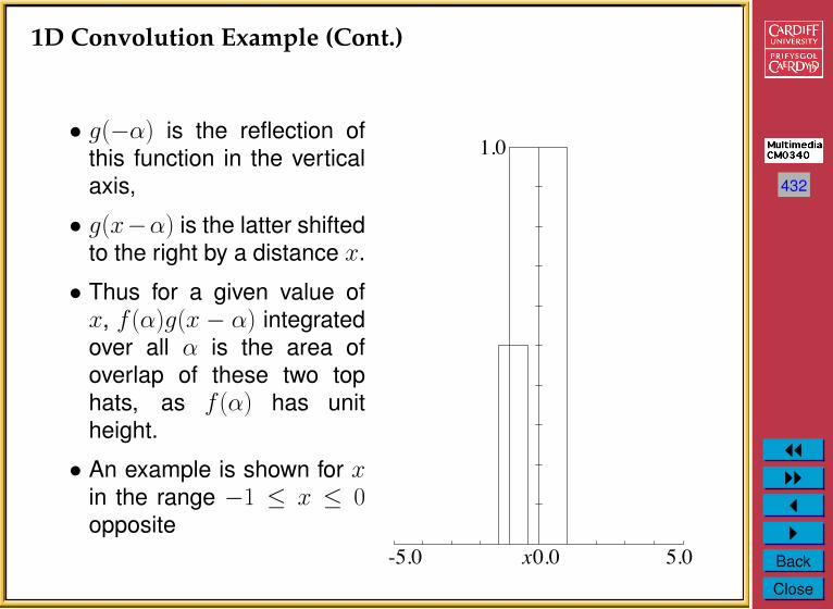
• g(−α) is the reflection ofthis function in the verticalaxis,

• g(x−α) is the latter shiftedto the right by a distance x.

• Thus for a given value ofx, f (α)g(x − α) integratedover all α is the area ofoverlap of these two tophats, as f (α) has unitheight.

• An example is shown for xin the range −1 ≤ x ≤ 0opposite

-5.0 5.00.0

1.0

x

433

JJIIJI

Back

Close

1D Convolution Example (cont.)

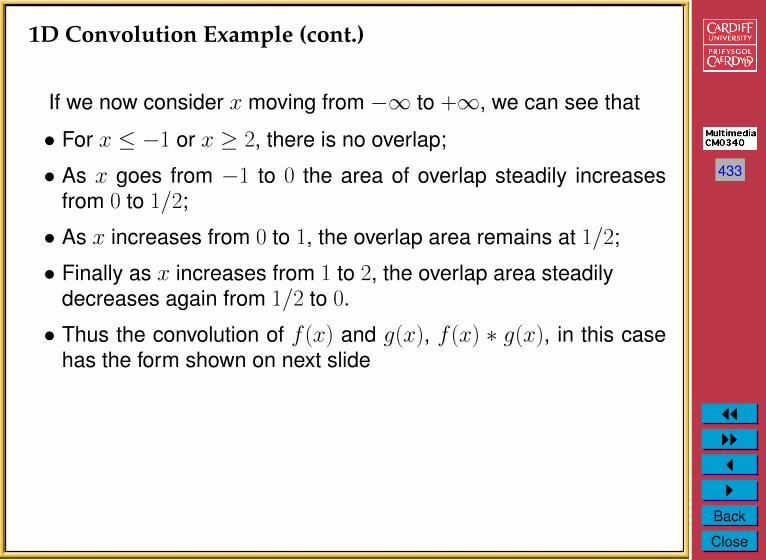
If we now consider x moving from −∞ to +∞, we can see that

• For x ≤ −1 or x ≥ 2, there is no overlap;

• As x goes from −1 to 0 the area of overlap steadily increasesfrom 0 to 1/2;

• As x increases from 0 to 1, the overlap area remains at 1/2;

• Finally as x increases from 1 to 2, the overlap area steadilydecreases again from 1/2 to 0.

• Thus the convolution of f (x) and g(x), f (x) ∗ g(x), in this casehas the form shown on next slide

434

JJIIJI

Back

Close

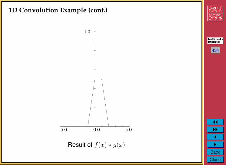
1D Convolution Example (cont.)

-5.0 5.00.0

1.0

Result of f (x) ∗ g(x)

435

JJIIJI

Back

Close

1D Convolution Example (cont.)

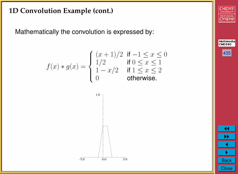
Mathematically the convolution is expressed by:

f (x) ∗ g(x) =

(x + 1)/2 if −1 ≤ x ≤ 01/2 if 0 ≤ x ≤ 11− x/2 if 1 ≤ x ≤ 20 otherwise.

-5.0 5.00.0

1.0

436

JJIIJI

Back

Close

Fourier Transforms and Convolutions

One major reason that Fourier transforms are so important in imageprocessing is the convolution theorem which states that:

If f (x) and g(x) are two functions with Fourier transforms F (u)and G(u), then the Fourier transform of the convolution f (x) ∗ g(x)is simply the product of the Fourier transforms of the two functions,F (u)G(u).

Recall our Low Pass Filter Example (MATLAB CODE)

% Apply filterG=H.*F;

Where F was the Fourier transform of the image, H the filter

437

JJIIJI

Back

Close

Computing Convolutions with the FourierTransformE.g.:

• To apply some reverb to an audio signal, example later

• To compensate for a less than ideal image capture system:

To do this fast convolution we simply:

• Take the Fourier transform of the audio/imperfect image,

• Take the Fourier transform of the function describing the effect ofthe system,

• Multiply by the effect to apply effect to audio data

• To remove/compensate for effect: Divide by the effect to obtainthe Fourier transform of the ideal image.

• Inverse Fourier transform to recover the new audio/ideal image.

This process is sometimes referred to as deconvolution.