05-LME-Ch05

151

Chapter FiveDemand for Labour in CompetitiveLabour Markets

Main Questions

• Labour demand functions are conventionally drawn asdownward sloping (i.e., decreasing functions of themarket wage). Is there any theoretical justification forthis convention? Is there corresponding empiricalsupport?

• Labour demand decisions are made bothsimultaneously with other input decisions and afterfactories and machines have been built. How do labourdemand decisions compare in these twocircumstances, (i.e., how do labour demand decisionsdiffer in the short and long run)?

• What factors affect the elasticity of demand for labour?For example, does it matter whether a firm operatesas a monopolist or a perfect competitor in the productmarket?

• How can we characterize the “competitiveness” ofCanadian labour in an increasingly globalized worldeconomy? How have the productivities and wages ofCanadian workers evolved over time compared to therest of the world?

• How can we use labour demand functions to assessthe impact of outsourcing and globalization on thewages and employment of Canadian workers?

The general principles that determine the demand for any factor of production applyalso to the demand for labour. In contrast to goods and services, factors of production aredemanded not for final use or consumption but as inputs into the production of final goodsand services. Thus the demand for a factor is necessarily linked to the demand for thegoods and services that the factor is used to produce. The demand for land suitable forgrowing wheat is linked to the demand for bread and cereal, just as the demand for con-struction workers is related to the demand for new buildings, roads, and bridges. For thisreason, the demand for factors is called a derived demand.

In discussing firms’ decisions regarding the employment of factors of production, econ-omists usually distinguish between short-run and long-run decisions. The short run isdefined as a period during which one or more factors of production—referred to as fixedfactors—cannot be varied, while the long run is defined as a period during which the firmcan adjust all of its inputs. During both the short and the long run, the state of technicalknowledge is assumed to be fixed; the very long run refers to the period during whichchanges in technical knowledge can occur. The amount of calendar time corresponding toeach of these periods will differ from one industry to another and according to other fac-tors. These periods are useful as a conceptual device for analyzing a firm’s decision-makingrather than for predicting the amount of time taken to adjust to change.

By the demand for labour we mean the quantity of labour services the firm wouldchoose to employ at each wage. This desired quantity will depend on both the firm’s objec-tives and its constraints. Usually we will assume that the firm’s objective is to maximizeprofits. Also examined is the determination of labour demand under the weaker assump-tion of cost minimization. The firm is constrained by the demand conditions in its productmarkets, the supply conditions in its factor markets, and its production function, whichshows the maximum output attainable for various combinations of inputs, given the exist-ing state of technical knowledge. In the short run the firm is further constrained by havingone or more factors of production whose quantities are fixed.

The theory of labour demand examines the quantity of labour services the firm desiresto employ given the market-determined wage rate, or given the labour supply function thatthe firm faces. As was the case with labour supply, our guiding objective is in deriving thetheoretical relationship between labour demand and the market wage, holding other fac-tors constant. In this chapter we will assume that the firm is a perfect competitor in thelabour market. In Chapter 7, we relax this assumption and explore the case where the firmfaces the entire market supply curve, and operates as a monopsonist. In that case, it makesno sense to think of the firm as reacting to a given market wage. However, as we shall see,the basic ingredients of the theory of input demand can easily be adjusted to this problem.

In some circumstances, however, it makes no sense to think of either the firm or thelabour it hires as operating in a competitive market. The employer and employees maynegotiate explicit, or reach implicit, contracts involving both wages and employment.When this is the case, the wage-employment outcomes may not be on the labour demandcurve because the contracts will reflect the preferences of both the employer and theemployees with respect to both wages and employment. Explicit wage-employment con-tracts are discussed in Chapter 15 on unions, and implicit wage-employment contracts arediscussed in Chapter 18 on unemployment (because of the theoretical links betweenimplicit contracts and unemployment). Even under these circumstances, however, we shallsee that the theory of firm behaviour described in this chapter is the foundation foremployment determination outside the perfectly competitive framework.

The chapter ends with an extended discussion on the impact of the global economy onthe demand for Canadian labour. The relative cost and productivity of Canadian labour isexamined, as are the possible channels by which outsourcing and changes in internationaltrade patterns may impact the employment of Canadian workers. In particular, we presentevidence on the impact of trade agreements (like NAFTA) on the Canadian labour market.

CATEGORIZING THE STRUCTURE OF PRODUCT AND LABOUR MARKETS

Because the demand for labour is derived from the output produced by the firm, the wayin which the firm behaves in the product market can have an impact on the demand forlabour, and hence ultimately on wage and employment decisions. In general, the firm’sproduct market behaviour depends on the structure of the industry to which the firmbelongs. In decreasing order of the degree of competition, the four main market structuresare (1) perfect competition, (2) monopolistic competition, (3) oligopoly, and (4) monopoly.

Whereas the structure of the product market affects the firm’s derived demand forlabour, the structure of the labour market affects the labour supply curve that the firmfaces. The supply curve of labour to an individual firm shows the amount of a specific typeof labour (e.g., a particular occupational category) that the firm could employ at variouswage rates. Analogous to the four product market structures there are four labour marketstructures. In decreasing order of the degree of competition the firm faces in hiring labour,these factor market structures are (1) perfect competition, (2) monopsonistic competition,

152 PART 2: Labour Demand

(3) oligopsony, and (4) monopsony. (The “-opsony” ending is traditionally used to denotedepartures from perfect competition in factor markets.)

The product and labour market categorizations are independent in that there is no nec-essary relationship between the structure of the product market in which the firm sells itsoutput and the labour market in which it buys labour services. The extent to which thefirm is competitive in the product market (and hence the nature of its derived demand forlabour curve) need not be related to the extent to which the firm is a competitive buyerof labour (and hence the nature of the supply curve of labour that it faces). The two maybe related, for example if it is a large firm and hence dominates both the labour and prod-uct markets, but they need not be related. Hence for each product market structure, thefirm can behave in at least four different ways as a purchaser of labour. Thus there are atleast 16 different combinations of product and labour market structure that can bear onthe wage and employment decision at the level of the firm.

In general, however, the essence of the wage and employment decision by the firm canbe captured by an examination of the polar cases of perfect competition (in productand/or factor markets), monopoly in the product market, and monopsony in the labourmarket. We will begin by examining the demand for labour in the short run under condi-tions of perfect competition in the labour market.

DEMAND FOR LABOUR IN THE SHORT RUN

The general principles determining labour demand can be explained for the case of a firmthat produces a single output (Q) using two inputs, capital (K), and labour (N). The tech-nological possibilities relating output to any combination of inputs are represented by theproduction function:

Q = F(K,N) (5.1)

In the short run the amount of capital is fixed at K = K0, so the production function is sim-ply a function of N (with K fixed). The quantity of labour services can be varied by chang-ing either the number of employees or hours worked by each employee (or both). For themoment we do not distinguish between variations in the number of employees and hoursworked; however, this aspect of labour demand is discussed in Chapter 6. Also discussedlater is the possibility that labour may be a “quasi-fixed factor” in the short run.

The demand for labour in the short run can be derived by examining the firm’s short-run output and employment decisions. Two decision rules follow from the assumption ofprofit maximization. First, because the costs associated with the fixed factor must bepaid whether or not the firm produces (and whatever amount the firm produces), the firmwill operate as long as it can cover its variable costs (i.e., if total revenue exceeds totalvariable costs). Fixed costs are sunk costs, and their magnitude should not affect what isthe currently most profitable thing to do.

The second decision rule implied by profit maximization is that, if the firm produces atall (i.e., is able to cover its variable costs), it should produce the quantity Q* at which mar-ginal revenue (MR) equals marginal cost (MC). That is, the firm should increase outputuntil the additional cost associated with the last unit produced equals the additional rev-enue associated with that unit.

If the firm is a price-taker, the marginal revenue of another unit sold is the prevailingmarket price. If the firm is a monopolist, or operates in a less than perfectly competitiveproduct market, marginal revenue will be a decreasing function of output (the price mustfall in order for additional units to be sold). With capital fixed, the marginal cost of pro-ducing another unit of output is the wage times the amount of labour required to producethat output. Expanding output beyond the point at which MR = MC will lower profits

153Chapter 5: Demand for Labour in Competitive Labour Markets

because the addition to total revenue will be less than the increase in total cost. Producinga lower output would also reduce profits because, at output levels below Q*, marginal rev-enue exceeds marginal cost; thus increasing output would add more to total revenue thanto total cost, thereby raising profits.

The profit-maximizing decision rules can be stated in terms of the employment of inputsrather than in terms of the quantity of output to produce. Because concepts such as totalrevenue and marginal revenue are defined in terms of units of output, the terminology ismodified for inputs. The total revenue associated with the amount of an input employed iscalled the total revenue product (TRP) of that input;similarly, the change in total revenueassociated with a change in the amount of the input employed is called the marginal rev-enue product (MRP). Both the total and marginal revenue products of labour will dependon the physical productivity of labour as given by the production function, and the mar-ginal revenue received from selling the output of the labour in the product market.

Thus the profit-maximizing decision rules for the employment of the variable input canbe stated as follows:

• The firm should produce, providing the total revenue product of the variable inputexceeds the total costs associated with that input; otherwise the firm should shutdown operations.

• If the firm produces at all, it should expand employment of the variable input to thepoint at which its marginal revenue product equals its marginal cost.

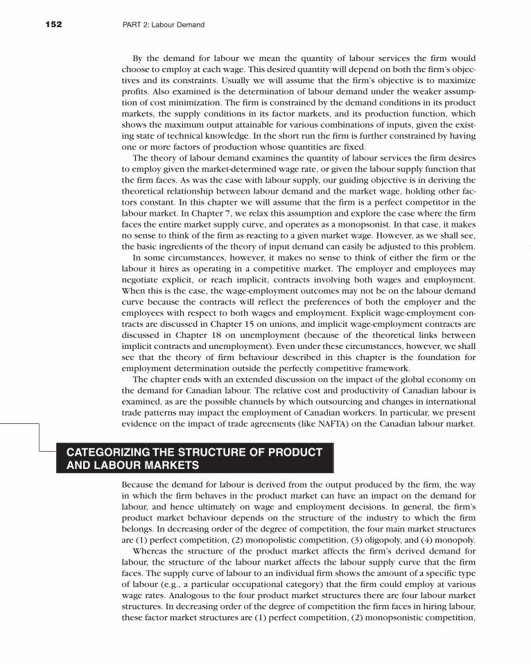
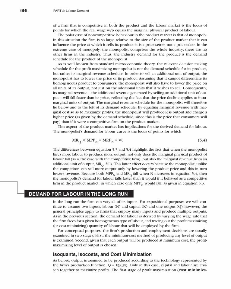
The short-run employment decision of a firm operating in a perfectly competitive labourmarket is shown in Figure 5.1. In a competitive factor market the firm is a price-taker; i.e.,the firm can hire more or less of the factor without affecting the market price. Thus in acompetitive labour market the marginal (and average) cost of labour is the market wagerate. The firm will therefore employ labour until its marginal revenue product equals thewage rate, which implies that the firm’s short-run labour demand curve is its marginal rev-enue product of labour curve. For example, if the wage rate is W0 the firm would employN0* labour services. However, the firm will shut down operations in the short run if thetotal variable cost exceeds the total revenue product of labour, which will be the case ifthe average cost of labour (the wage rate) exceeds the average revenue product of labour(ARP). Thus at wage rates higher than W1 in Figure 5.1 (the point at which the wage rateequals the average product of labour) the firm would choose to shut down operations. Itfollows that the firm’s short-run labour demand curve is its marginal revenue product oflabour curve below the point at which the average and marginal product curves intersect(i.e., below the point at which the ARPN reaches a maximum).

The short-run labour demand curve is downward sloping because of diminishingmarginal returns to labour. Although the average and marginal products may initially riseas more labour is employed, both eventually decline as more units of the variable factor arecombined with a given amount of the fixed factor. Because the firm employs labour in therange in which its marginal revenue product is declining, a reduction in the wage rate isneeded to entice the firm to employ more labour. Similarly, an increase in the wage rate willcause the firm to employ less labour, thus raising its marginal revenue product and restoringequality between the marginal revenue product and marginal cost.

At this point, it may be worth highlighting a common misconception concerning the rea-son for the downward-sloping demand for labour. The demand is for a given homogeneoustype of labour; consequently, it does not slope downward because, as the firm uses morelabour, it uses poorer-quality labour and hence pays a lower wage. It may well be true thatwhen firms expand their work force they often have to use poorer-quality labour.Nevertheless, for analytical purposes it is useful to assume a given, homogeneous type oflabour so that the impact on labour demand of changes in the wage rate for that type oflabour can be analyzed. The change in the productivity of labour that occurs does so because


of changes in the amount of the variable factor combined with a given amount of the fixedfactor, not because the firm is utilizing inferior labour.

WAGES, THE MARGINAL PRODUCTIVITY OF LABOUR,AND COMPETITION IN THE PRODUCT MARKET

The demand schedule of a profit-maximizing firm that is a wage-taker in the labour marketis the locus of points for which the marginal revenue product of labour equals the wagerate. The marginal revenue product of labour (MRPN) equals the marginal revenue of out-put (MRQ) times the marginal physical product of labour (MPPN). Thus there is a rela-tionship between wages and the marginal productivity of labour.

The marginal revenue of output depends on the market structure in the product market.The two polar cases of perfect competition and monopoly are discussed here. A perfectlycompetitive firm is a price-taker in the product market. Because the firm can sell additional(or fewer) units of output without affecting the market price, the marginal revenue of out-put equals the product price; i.e., for a competitive firm

MRPN = MRQ � MPPN = p � MPPN (5.2)

Because it is the product of the market price and the marginal product of labour, thisMPPN term is also sometimes called the value of the marginal product of labour. A firmthat is competitive in both the product and the labour market will thus employ labour serv-ices until the value of the marginal product of labour just equals the wage; i.e., the demandfor labour obeys the equation 5.3:

p � MPPN = MRPN = w (5.3)

Equation 5.3 follows from the MR = MC rule for profit maximization; the MRPN is theincrease in total revenue associated with a unit increase in labour input, while the wage wis the accompanying increase in total cost. Alternatively stated, the labour demand curve


MRPNARPN

N* N*

W1

W0

Wage rate

Employment1 0

Figure 5.1Profit maximizationrequires labour tobe employed untilits marginal cost(the wage) equals itsmarginal benefit(marginal revenueproduct). For thewage, W0, the profit-maximizing employ-ment level is N *0. Atwages higher thanW1, labour costsexceed the value ofoutput, so the firmwill hire no labour.The labour demandschedule is thusMRPN below whereARPN reaches itsmaximum (thethicker part of thecurve on the figure).

The Firm’s Short-Run Demand for Labour

of a firm that is competitive in both the product and the labour market is the locus ofpoints for which the real wage w/p equals the marginal physical product of labour.

The polar case of noncompetitive behaviour in the product market is that of monopoly.In this situation the firm is so large relative to the size of the product market that it caninfluence the price at which it sells its product: it is a price-setter, not a price-taker. In theextreme case of monopoly, the monopolist comprises the whole industry: there are noother firms in the industry. Thus, the industry demand for the product is the demandschedule for the product of the monopolist.

As is well known from standard microeconomic theory, the relevant decision-makingschedule for the profit-maximizing monopolist is not the demand schedule for its product,but rather its marginal revenue schedule. In order to sell an additional unit of output, themonopolist has to lower the price of its product. Assuming that it cannot differentiate itshomogeneous product to consumers, the monopolist will also have to lower the price onall units of its output, not just on the additional units that it wishes to sell. Consequently,its marginal revenue—the additional revenue generated by selling an additional unit of out-put—will fall faster than its price, reflecting the fact that the price decline applies to intra-marginal units of output. The marginal revenue schedule for the monopolist will thereforelie below and to the left of its demand schedule. By equating marginal revenue with mar-ginal cost so as to maximize profits, the monopolist will produce less output and charge ahigher price (as given by the demand schedule, since this is the price that consumers willpay) than if it were a competitive firm on the product market.

This aspect of the product market has implications for the derived demand for labour.The monopolist’s demand for labour curve is the locus of points for which

MRQ � MPPN = MRPN = w. (5.4)

The differences between equation 5.3 and 5.4 highlight the fact that when the monopolisthires more labour to produce more output, not only does the marginal physical product oflabour fall (as is the case with the competitive firm), but also the marginal revenue from anadditional unit of output, MRQ, falls. This latter effect occurs because the monopolist, unlikethe competitor, can sell more output only by lowering the product price and this in turnlowers revenue. Because both MPPN and MRQ fall when N increases in equation 5.4, thenthe monopolist’s demand for labour falls faster than it would if it behaved as a competitivefirm in the product market, in which case only MPPN would fall, as given in equation 5.3.

DEMAND FOR LABOUR IN THE LONG RUN

In the long run the firm can vary all of its inputs. For expositional purposes we will con-tinue to assume two inputs, labour (N) and capital (K) and one output (Q); however, thegeneral principles apply to firms that employ many inputs and produce multiple outputs.As in the previous section, the demand for labour is derived by varying the wage rate thatthe firm faces for a given homogeneous type of labour, and tracing out the profit-maximizing(or cost-minimizing) quantity of labour that will be employed by the firm.

For conceptual purposes, the firm’s production and employment decisions are usuallyexamined in two stages. First, the minimum-cost method of producing any level of outputis examined. Second, given that each output will be produced at minimum cost, the profit-maximizing level of output is chosen.

Isoquants, Isocosts, and Cost MinimizationAs before, output is assumed to be produced according to the technology represented bythe firm’s production function, Q = F(K,N). Only in this case, capital and labour are cho-sen together to maximize profits. The first stage of profit maximization (cost minimiza-


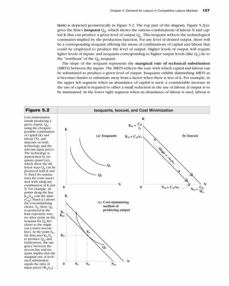
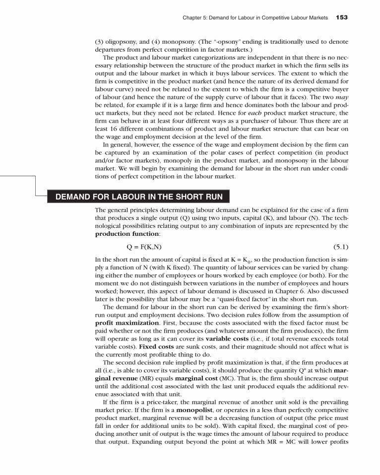
tion) is depicted geometrically in Figure 5.2. The top part of the diagram, Figure 5.2(a),gives the firm’s isoquant Q0, which shows the various combinations of labour N and cap-ital K that can produce a given level of output Q0. This isoquant reflects the technologicalconstraints implied by the production function. For any level of desired output, there willbe a corresponding isoquant offering the menu of combinations of capital and labour thatcould be employed to produce the level of output. Higher levels of output will requirehgher levels of inputs, and isoquants corresponding to higher output levels (like Q1) lie tothe “northeast” of the Q0 isoquant.

The slope of the isoquant represents the marginal rate of technical substitution(MRTS) between the inputs. The MRTS reflects the ease with which capital and labour canbe substituted to produce a given level of output. Isoquants exhibit diminishing MRTS asit becomes harder to substitute away from a factor when there is less of it. For example, inthe upper left segment when an abundance of capital is used, a considerable increase inthe use of capital is required to offset a small reduction in the use of labour, if output is tobe maintained. In the lower right segment when an abundance of labour is used, labour is


K

0N

K

0N

•

K

0N

(a) Isoquants

Q1

Q0

NM = CM/w0

KM = CM/r0

Slope = –w0 /r

0

(b) Isocost

(c) Cost-minimizing method of producing output

Q0

E0

KM

K0

K1

N0N1 NM

CH

W0NH =

CH

r0KH =

•

Figure 5.2Cost minimizationentails producing agiven output, Q0,using the cheapestpossible combinationof capital (K) andlabour (N), anddepends on bothtechnology and therelevant input prices.The technology isrepresented by iso-quants (panel (a)),which show the dif-ferent ways Q0 can beproduced with K andN. Panel (b) summa-rizes the costs associ-ated with using anycombination of K andN. For example, allpoints along the lineKMNM cost the same(CM). Panel (c) showsthe cost-minimizingchoice, E0. Here, Q0is produced in theleast expensive way:no other point on theisoquant for Q0 liescloser to the origin(on a lower isocostline). At the point E0,the firm uses K0,N0to produce Q0, and,furthermore, the tan-gency between theisocost line and iso-quant implies that themarginal rate of tech-nical substitutionequals the ratio ofinput prices (W0/r0).

Isoquants, Isocost, and Cost Minimization

a poor substitute for capital, and considerable labour savings are possible for smallincreases in the use of capital. In the middle segment of the isoquant, labour and capitalare both good substitutes. Successively higher isoquants or levels of output, such as Q1, canbe produced by successively larger amounts of both inputs.

Clearly, under differing technologies, we expect the difficulty of substitution to vary. Ifhoeing requires one hoe per worker, purchasing additional hoes without the workers, orhiring extra workers without hoes, will not allow much of an increase in output. In thatcase, production would be characterized by a low level of substitutability between theinputs. On the other hand, it might be easier to substitute weeding labour for herbicides.One could imagine using a lot of labour, doing all the weeding by hand, or hiring only oneworker to apply large quantities of chemicals. Intermediate combinations would also befeasible. In that case, the level of substitutability will be high. The substitutability of onefactor for another will clearly have an effect on the responsiveness of producers to smallchanges in the relative prices of the two factors.

The firm’s objective will be to choose the least expensive combination of capital andlabour along the isoquant Q0. The costs of purchasing various combinations of capital andlabour will depend on the prices of the inputs. Figure 5.2(b) illustrates the firm’s isocostline KMNM, depicting the various combinations of capital and labour the firm can employ, given their market price and a total cost of CM. Algebraically, the isocost line is CM = rK + wN,where r is the price of capital and w the price of labour, or wage rate.1 The position and shapeof the isocost line can be determined by solving for the two intercepts or endpoints and theslope of the line between them. From the isocost equation, for fixed prices r0 and w0, theseendpoints are NM = CM/w0 when K = 0, and KM = CM/r0 when N = 0. The slope is simplyminus the rise divided by the run or �[CM/r0 � CM/w0] = �w0/r0; that is, the price of labourrelative to the price of capital. This is a straight line as long as w and r are constant for thesegiven types of labour and capital, which is the case when the firm is a price-taker in bothinput markets. Isocost lines will pass through each possible combination of capital and labourthat the firm could hire. For example, a higher isocost line, KHNH, is also depicted in Figure5.2(b). Costs are increasing as the isocost lines move to the northeast (away from the origin).

A profit-maximizing firm will choose the cheapest capital-labour combination that yieldsthe output Q0. In other words, it will choose the combination of K and N on the isoquantQ0 that lies on the isocost line nearest the origin. Figure 5.2(c) combines the isoquants andisocost lines to illustrate the minimum-cost input choice that can be used to produce Q0.This is clearly E0 where the isocost is tangent to the isoquant. That this should be theminimum-cost combination is most easily seen by considering an alternative combination,K1 and N1. The isocost line corresponding to this combination is associated with a highertotal cost of production. In this case, costs could be reduced by using more labour and lesscapital, and moving toward the combination at E0.

As with the consumer optimum described in Chapter 2, the tangency between the iso-quant and isocost lines has an economic interpretation. At the optimum for the firm, theinternal rate of input substitution, given by the marginal rate of technical substitution (theslope of the isoquant) equals the market rate of substitution, given by the relative price oflabour and capital (the slope of the isocost line). This tangency can also be expressed interms of the relative marginal products of capital and labour:

(5.5)MRTS =MPPN

MPPK

=w

r


1If the firm rents its capital equipment, the cost of capital is the rental price. If the firm owns its capital equip-ment, the implicit or opportunity cost of capital depends on the cost of the machinery and equipment, theinterest rate at which funds can be borrowed or lent, and the rate at which the machinery depreciates. In theanalysis that follows, we will assume that the firm is a price-taker in the market for capital.

In the short run, we saw that the value of the marginal product of labour was equal to thewage. In the long run, the relative value of the marginal product of labour is equal to therelative price of labour.

The second stage of profit maximization entails the choice of the optimal level of out-put. The determination of the profit-maximizing level of output (the output at which mar-ginal revenue equals marginal cost) cannot be seen in the isoquant-isocost diagram. Whatis shown is how to produce any output, including the profit-maximizing output, at mini-mum cost.

At E0, the cost-minimizing amounts of labour and capital, respectively used to produceQ0 units of output, are N0 and K0. If Q0 is the profit-maximizing output, this gives us onepoint on the demand curve for labour, as depicted later in Figure 5.3; that is, at the wagerate w0 the firm employs N0 units of labour.

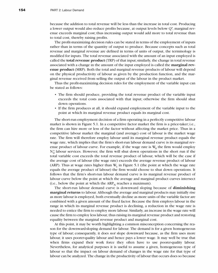
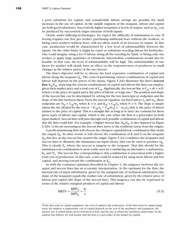
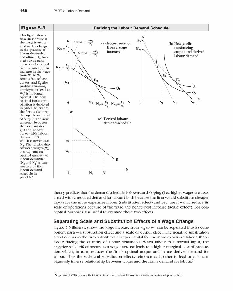
Deriving the Firm’s Labour Demand ScheduleThe complete labour demand schedule, for the long run when the firm can vary both cap-ital and labour, can be obtained simply by varying the wage rate and tracing out the new,equilibrium, profit-maximizing amounts of labour that would be employed. This is illus-trated in Figure 5.3. An increase in the wage from W0 to W1 causes all of the isocost curvesto become steeper. For example, at the initial input combination, K0 and N0, the isocostline rotates from KMNM to KPNP. Clearly, the total cost of continuing to produce Q0 usingK0 and N0 will rise. If the firm chose to rent only capital at the new cost level, C1, it wouldbe able to rent more capital services than before, up to KP = C1/r0. On the other hand, eventhough costs have risen, if the firm spent C1 entirely on labour, it could hire only up to NP= C1/W1. Finally, panel (a) shows that the cost-minimizing (and profit-maximizing) condi-tion no longer holds at E0, because the isoquant is not tangent to the new isocost line.

As depicted in Figure 5.3(b), given the higher wage rate W1, the firm will maximize prof-its by moving to a lower level of output Q1, operating at E1 and employing N1 units oflabour. This yields a second point on the firm’s demand curve for labour depicted in Figure5.3(c); that is, a lower level of employment N1 corresponds to the higher wage rate W1,compared to the original employment of N0 at wage w0.

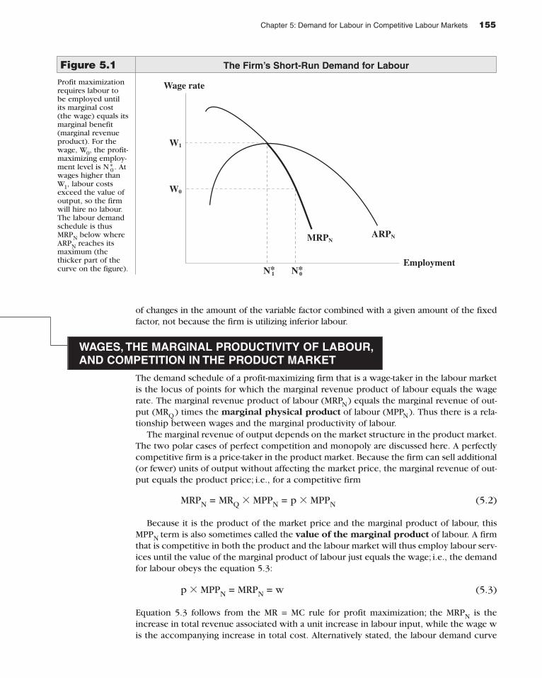
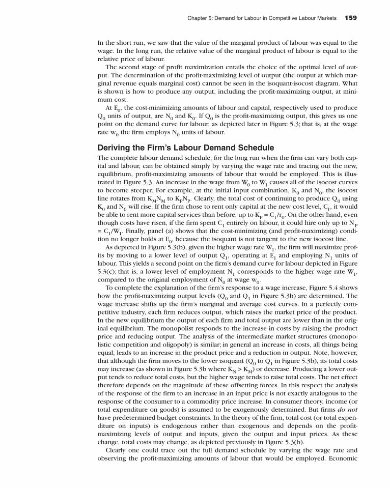
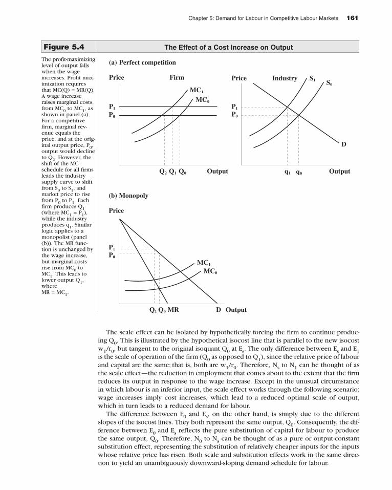
To complete the explanation of the firm’s response to a wage increase, Figure 5.4 showshow the profit-maximizing output levels (Q0 and Q1 in Figure 5.3b) are determined. Thewage increase shifts up the firm’s marginal and average cost curves. In a perfectly com-petitive industry, each firm reduces output, which raises the market price of the product.In the new equilibrium the output of each firm and total output are lower than in the orig-inal equilibrium. The monopolist responds to the increase in costs by raising the productprice and reducing output. The analysis of the intermediate market structures (monopo-listic competition and oligopoly) is similar; in general an increase in costs, all things beingequal, leads to an increase in the product price and a reduction in output. Note, however,that although the firm moves to the lower isoquant (Q0 to Q1 in Figure 5.3b), its total costsmay increase (as shown in Figure 5.3b where KN > KM) or decrease. Producing a lower out-put tends to reduce total costs, but the higher wage tends to raise total costs. The net effecttherefore depends on the magnitude of these offsetting forces. In this respect the analysisof the response of the firm to an increase in an input price is not exactly analogous to theresponse of the consumer to a commodity price increase. In consumer theory, income (ortotal expenditure on goods) is assumed to be exogenously determined. But firms do nothave predetermined budget constraints. In the theory of the firm, total cost (or total expen-diture on inputs) is endogenous rather than exogenous and depends on the profit-maximizing levels of output and inputs, given the output and input prices. As thesechange, total costs may change, as depicted previously in Figure 5.3(b).

Clearly one could trace out the full demand schedule by varying the wage rate andobserving the profit-maximizing amounts of labour that would be employed. Economic


theory predicts that the demand schedule is downward sloping (i.e., higher wages are asso-ciated with a reduced demand for labour) both because the firm would substitute cheaperinputs for the more expensive labour (substitution effect) and because it would reduce itsscale of operations because of the wage and hence cost increase (scale effect). For con-ceptual purposes it is useful to examine these two effects.

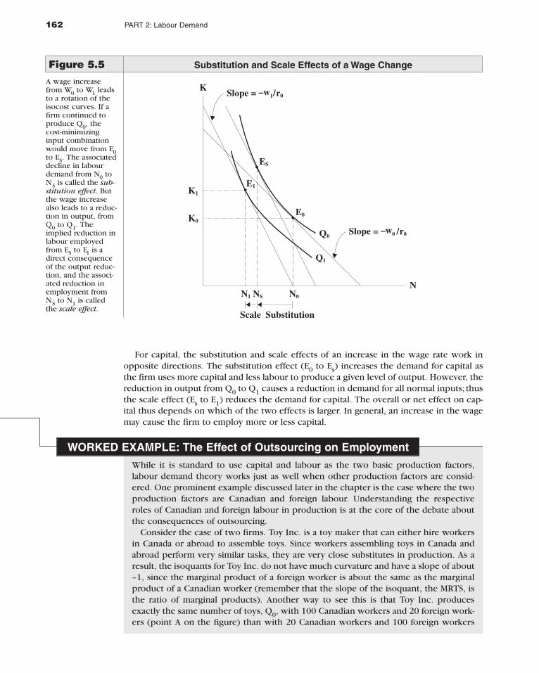
Separating Scale and Substitution Effects of a Wage ChangeFigure 5.5 illustrates how the wage increase from w0 to w1 can be separated into its com-ponent parts—a substitution effect and a scale or output effect. The negative substitutioneffect occurs as the firm substitutes cheaper capital for the more expensive labour, there-fore reducing the quantity of labour demanded. When labour is a normal input, thenegative scale effect occurs as a wage increase leads to a higher marginal cost of produc-tion which, in turn, reduces the firm’s optimal output and hence derived demand forlabour. Thus the scale and substitution effects reinforce each other to lead to an unam-biguously inverse relationship between wages and the firm’s demand for labour.2


W

0N

K

0N

KN

KM

E1

E0

N0

Q0

Q1

N1 NM

(b) New profit- maximizing output and derived labour demand

(c) Derived labour demand schedule

D

N1 N0

w1

w0

0 N0

K0E0

Q0

N

K

KP = C1

r0

NP = C1

w1

Slope = –w1

r0(a) Isocost rotation from a wage increaseSlope =

–w0

r0

NM = C0

w0

KM = C0

r0

•

•

•

•

••

•

Figure 5.3This figure showshow an increase inthe wage is associ-ated with a changein the quantity oflabour demanded,and ultimately, howa labour demandcurve can be tracedout. In panel (a), anincrease in the wagefrom W0 to W1rotates the isocostcurves, and E0 (theprofit-maximizingemployment level atW0) is no longeroptimal. The newoptimal input com-bination is depictedin panel (b), wherethe firm is also pro-ducing a lower levelof output. The newtangency betweenthe isoquant (forQ1) and isocostcurve yields labourdemand of N1,which is lower thanN0. The relationshipbetween wages (W0and W1) and theoptimal quantity oflabour demanded(N0 and N1) is sum-marized by thelabour demandschedule in panel (c).

Deriving the Labour Demand Schedule

2Nagatani (1978) proves that this is true even when labour is an inferior factor of production.

The scale effect can be isolated by hypothetically forcing the firm to continue produc-ing Q0. This is illustrated by the hypothetical isocost line that is parallel to the new isocostw1/r0, but tangent to the original isoquant Q0 at Es. The only difference between Es and E1is the scale of operation of the firm (Q0 as opposed to Q1), since the relative price of labourand capital are the same; that is, both are w1/r0. Therefore, Ns to N1 can be thought of asthe scale effect—the reduction in employment that comes about to the extent that the firmreduces its output in response to the wage increase. Except in the unusual circumstancein which labour is an inferior input, the scale effect works through the following scenario:wage increases imply cost increases, which lead to a reduced optimal scale of output,which in turn leads to a reduced demand for labour.

The difference between E0 and Es, on the other hand, is simply due to the differentslopes of the isocost lines. They both represent the same output, Q0. Consequently, the dif-ference between E0 and Es reflects the pure substitution of capital for labour to producethe same output, Q0. Therefore, N0 to Ns can be thought of as a pure or output-constantsubstitution effect, representing the substitution of relatively cheaper inputs for the inputswhose relative price has risen. Both scale and substitution effects work in the same direc-tion to yield an unambiguously downward-sloping demand schedule for labour.


Price Firm

Output

Price

Output

Price Industry

Output

MC1

MC0

Q1Q2 Q0

P1

P0

(a) Perfect competition

S1 S0

D

q1 q0

P1

P0

(b) Monopoly

P1

P0

MC1

MC0

Q1 Q0 MR D

Figure 5.4The profit-maximizinglevel of output fallswhen the wageincreases. Profit max-imization requiresthat MC(Q) = MR(Q). A wage increaseraises marginal costs,from MC0 to MC1, asshown in panel (a).For a competitivefirm, marginal rev-enue equals theprice, and at the orig-inal output price, P0,output would declineto Q2. However, theshift of the MCschedule for all firmsleads the industrysupply curve to shiftfrom S0 to S1, andmarket price to risefrom P0 to P1. Eachfirm produces Q1(where MC1 = P1),while the industryproduces q1. Similarlogic applies to amonopolist (panel(b)). The MR func-tion is unchanged bythe wage increase,but marginal costsrise from MC0 toMC1. This leads tolower output Q1,where MR = MC1.

The Effect of a Cost Increase on Output

For capital, the substitution and scale effects of an increase in the wage rate work inopposite directions. The substitution effect (E0 to Es) increases the demand for capital asthe firm uses more capital and less labour to produce a given level of output. However, thereduction in output from Q0 to Q1 causes a reduction in demand for all normal inputs; thusthe scale effect (Es to E1) reduces the demand for capital. The overall or net effect on cap-ital thus depends on which of the two effects is larger. In general, an increase in the wagemay cause the firm to employ more or less capital.

WORKED EXAMPLE: The Effect of Outsourcing on Employment

While it is standard to use capital and labour as the two basic production factors,labour demand theory works just as well when other production factors are consid-ered. One prominent example discussed later in the chapter is the case where the twoproduction factors are Canadian and foreign labour. Understanding the respectiveroles of Canadian and foreign labour in production is at the core of the debate aboutthe consequences of outsourcing.

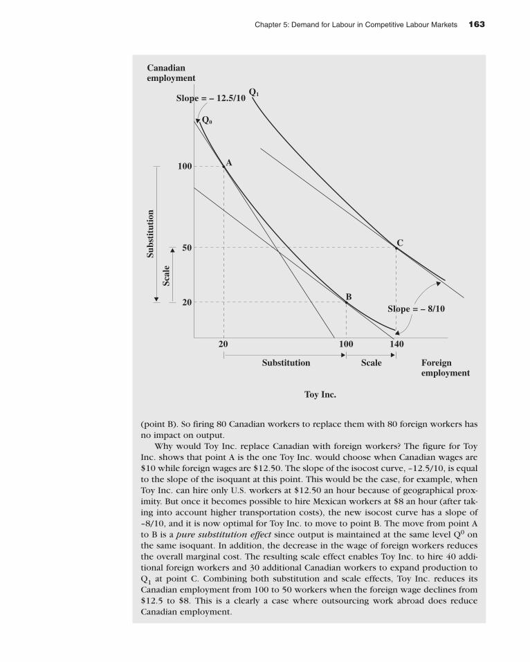
Consider the case of two firms. Toy Inc. is a toy maker that can either hire workersin Canada or abroad to assemble toys. Since workers assembling toys in Canada andabroad perform very similar tasks, they are very close substitutes in production. As aresult, the isoquants for Toy Inc. do not have much curvature and have a slope of about–1, since the marginal product of a foreign worker is about the same as the marginalproduct of a Canadian worker (remember that the slope of the isoquant, the MRTS, isthe ratio of marginal products). Another way to see this is that Toy Inc. producesexactly the same number of toys, Q0, with 100 Canadian workers and 20 foreign work-ers (point A on the figure) than with 20 Canadian workers and 100 foreign workers


Slope = –w1/r0

Slope = –w0 /r0

ES

E0

E1

Q0

Q1

N1 NS N0

N

K

K1

K0

Scale Substitution

•

•

•

Figure 5.5A wage increasefrom W0 to W1 leadsto a rotation of theisocost curves. If afirm continued toproduce Q0, thecost-minimizinginput combinationwould move from E0to ES. The associateddecline in labourdemand from N0 toNS is called the sub-stitution effect. Butthe wage increasealso leads to a reduc-tion in output, fromQ0 to Q1. Theimplied reduction inlabour employedfrom ES to E1 is adirect consequenceof the output reduc-tion, and the associ-ated reduction inemployment fromNS to N1 is calledthe scale effect.

Substitution and Scale Effects of a Wage Change


(point B). So firing 80 Canadian workers to replace them with 80 foreign workers hasno impact on output.

Why would Toy Inc. replace Canadian with foreign workers? The figure for ToyInc. shows that point A is the one Toy Inc. would choose when Canadian wages are$10 while foreign wages are $12.50. The slope of the isocost curve, –12.5/10, is equalto the slope of the isoquant at this point. This would be the case, for example, whenToy Inc. can hire only U.S. workers at $12.50 an hour because of geographical prox-imity. But once it becomes possible to hire Mexican workers at $8 an hour (after tak-ing into account higher transportation costs), the new isocost curve has a slope of–8/10, and it is now optimal for Toy Inc. to move to point B. The move from point Ato B is a pure substitution effect since output is maintained at the same level Q0 onthe same isoquant. In addition, the decrease in the wage of foreign workers reducesthe overall marginal cost. The resulting scale effect enables Toy Inc. to hire 40 addi-tional foreign workers and 30 additional Canadian workers to expand production toQ1 at point C. Combining both substitution and scale effects, Toy Inc. reduces itsCanadian employment from 100 to 50 workers when the foreign wage declines from$12.5 to $8. This is a clearly a case where outsourcing work abroad does reduceCanadian employment.

Q1

Q0

A100

Slope = – 12.5/10

Slope = – 8/10

50

20

20 100 140

B

C•

•

•

Scal

e

Subs

titu

tion

Canadianemployment

Toy Inc.

Scale Foreignemployment

Substitution

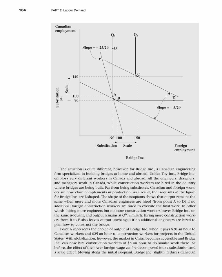
The situation is quite different, however, for Bridge Inc., a Canadian engineeringfirm specialized in building bridges at home and abroad. Unlike Toy Inc., Bridge Inc.employs very different workers in Canada and abroad. All the engineers, designers,and managers work in Canada, while construction workers are hired in the countrywhere bridges are being built. Far from being substitutes, Canadian and foreign work-ers are now close complements in production. As a result, the isoquants in the figurefor Bridge Inc. are L-shaped. The shape of the isoquants shows that output remains thesame when more and more Canadian engineers are hired (from point A to D) if noadditional foreign construction workers are hired to execute the final work. In otherwords, hiring more engineers but no more construction workers leaves Bridge Inc. onthe same isoquant, and output remains at Q0. Similarly, hiring more construction work-ers from B to E also leaves output unchanged if no additional engineers are hired toplan how to construct the bridge.

Point A represents the choice of output of Bridge Inc. when it pays $20 an hour toCanadian workers and $25 an hour to construction workers for projects in the UnitedStates. With globalization, however, the market in China becomes accessible and BridgeInc. can now hire construction workers at $5 an hour to do similar work there. Asbefore, the effect of the lower foreign wage can be decomposed into a substitution anda scale effect. Moving along the initial isoquant, Bridge Inc. slightly reduces Canadian


Q1Q0

A

140

Slope = – 25/20

Slope = – 5/20

10090

90 100 150

B

D

E

C

• •

•

•

•

Scal

e

Subs

titu

tion

Canadianemployment

Bridge Inc.

Scale Foreignemployment

Substitution

employment from 100 to 90 workers (point B) and increases foreign employment from90 to 100 when the foreign wage falls from $25 an hour to $5 an hour. But the lowerforeign wage reduces marginal costs, which leads to an expansion of output to pointC. Bridge Inc. hires 50 additional Canadian workers and 50 additional foreign workersas a result of this scale effect. In the end, the adverse impact of the substitution effecton Canadian employment (10 jobs) is more than offset by the scale effect (50 jobs). Thefact that Bridge Inc. employs more foreign workers than before (150 instead of 90) doesnot result in a decline of Canadian employment. Globalization and outsourcing maythus be good or bad for Canadian employment. Everything depends on whetherCanadian and foreign workers are substitutes or complements in production.

THE RELATIONSHIP BETWEEN THE SHORT- AND THE LONG-RUN LABOUR DEMAND

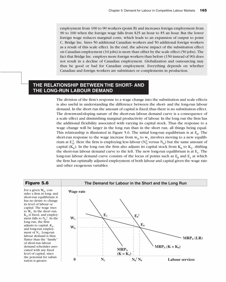
The division of the firm’s response to a wage change into the substitution and scale effectsis also useful in understanding the difference between the short- and the long-run labourdemand. In the short run the amount of capital is fixed; thus there is no substitution effect.The downward-sloping nature of the short-run labour demand curve is a consequence ofa scale effect and diminishing marginal productivity of labour. In the long run the firm hasthe additional flexibility associated with varying its capital stock. Thus the response to awage change will be larger in the long run than in the short run, all things being equal.This relationship is illustrated in Figure 5.6. The initial long-run equilibrium is at E0. Theshort-run response to the wage increase from w0 to w1 involves moving to a new equilib-rium at E 1

0. Here the firm is employing less labour (N10 versus N0) but the same amount of

capital (K0). In the long run the firm also adjusts its capital stock from K0 to K1, shiftingthe short-run labour demand curve to the left. The new long-run equilibrium is at E1. Thelong-run labour demand curve consists of the locus of points such as E0 and E1 at whichthe firm has optimally adjusted employment of both labour and capital given the wage rateand other exogenous variables.


Wage rate

W1

W0

0 N1 N01 N0 Labour services

E1 E01

E0

MRPN

(K = K1)

MRPN (K = K0)

MRPN (LR)

Figure 5.6For a given W0, con-sider a firm in long- andshort-run equilibrium: ithas no desire to changeits level of labour orcapital. The wage risesto W1. In the short run,K0 is fixed, and employ-ment falls to N0

1. In thelong run, the firmadjusts to capital, K1,and long-run employ-ment of N1. Long-runlabour demand is thusflatter than the “family”of short-run labourdemand schedules asso-ciated with any fixedlevel of capital, sincethe potential for substi-tution is greater.

The Demand for Labour in the Short and the Long Run

LABOUR DEMAND UNDER COST MINIMIZATION

Economic analysis generally assumes that firms in the private sector seek to maximize prof-its. However, organizations in the public and quasi-public sectors—such as federal, provin-cial, and municipal public administration, Crown corporations, and educational and healthinstitutions—generally have other goals. These goals will determine the quantity of outputor services provided and the amount of labour and other productive inputs employed.Although the factors that determine the output of these organizations may vary, suchorganizations may seek to produce that output efficiently, that is, at minimum cost.

The distinction between the scale and substitution effects is useful in analyzing thedemand for labour in these circumstances. An organization whose output of goods and/orservices is exogenously determined but that seeks to produce that output at minimum costwill respond to changes in wages by substituting between labour and other inputs. That is,with output fixed (determined by other factors) there will be a pure substitution effect inresponse to changes in the wage rate. Labour demand will therefore be unambiguouslydownward sloping but more inelastic than that of a profit-maximizing firm because of theabsence of an output effect.

Although a cost-minimizing organization will respond to a wage increase by substitutingcapital for labour, its total expenditure on inputs (total costs) will nonetheless rise. Thisaspect is illustrated in Figure 5.5. The equilibrium Es involves greater total costs than theoriginal equilibrium E0. The increase in total costs is, however, less than would be the caseif the organization did not substitute capital for labour in response to the wage increase(i.e., if the firm remained at the point E0 in Figure 5.5).

ELASTICITY OF DEMAND FOR LABOUR

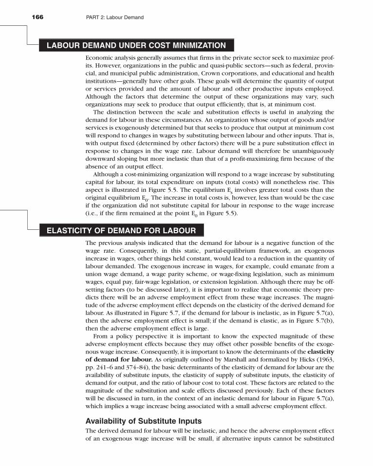
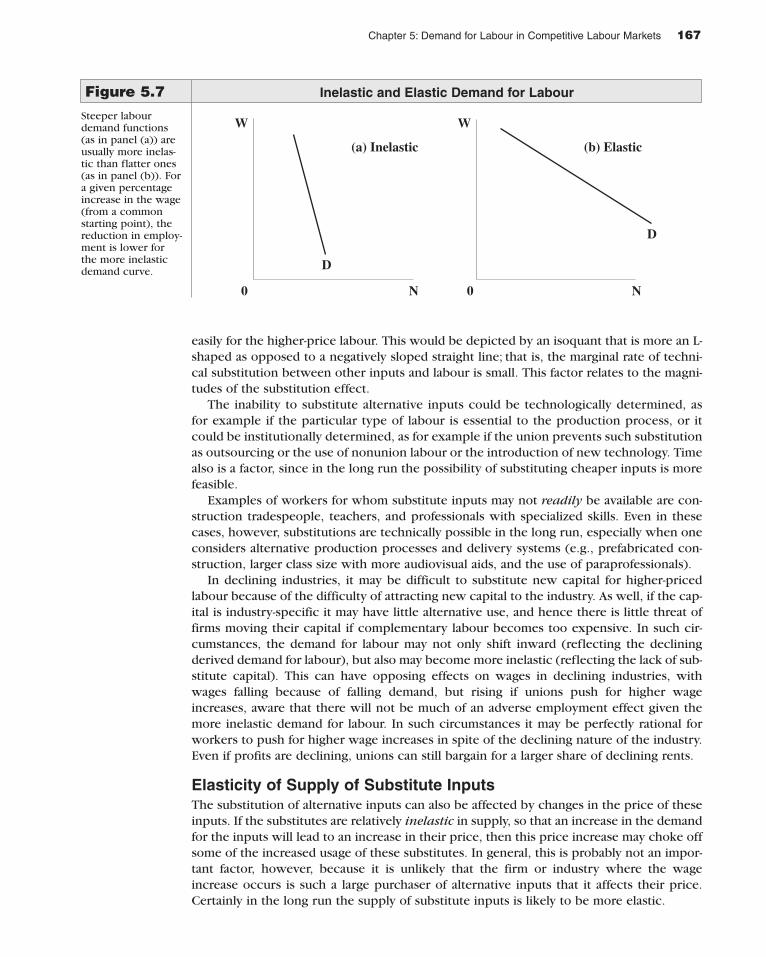
The previous analysis indicated that the demand for labour is a negative function of thewage rate. Consequently, in this static, partial-equilibrium framework, an exogenousincrease in wages, other things held constant, would lead to a reduction in the quantity oflabour demanded. The exogenous increase in wages, for example, could emanate from aunion wage demand, a wage parity scheme, or wage-fixing legislation, such as minimumwages, equal pay, fair-wage legislation, or extension legislation. Although there may be off-setting factors (to be discussed later), it is important to realize that economic theory pre-dicts there will be an adverse employment effect from these wage increases. The magni-tude of the adverse employment effect depends on the elasticity of the derived demand forlabour. As illustrated in Figure 5.7, if the demand for labour is inelastic, as in Figure 5.7(a),then the adverse employment effect is small; if the demand is elastic, as in Figure 5.7(b),then the adverse employment effect is large.

From a policy perspective it is important to know the expected magnitude of theseadverse employment effects because they may offset other possible benefits of the exoge-nous wage increase. Consequently, it is important to know the determinants of the elasticityof demand for labour. As originally outlined by Marshall and formalized by Hicks (1963,pp. 241–6 and 374–84), the basic determinants of the elasticity of demand for labour are theavailability of substitute inputs, the elasticity of supply of substitute inputs, the elasticity ofdemand for output, and the ratio of labour cost to total cost. These factors are related to themagnitude of the substitution and scale effects discussed previously. Each of these factorswill be discussed in turn, in the context of an inelastic demand for labour in Figure 5.7(a),which implies a wage increase being associated with a small adverse employment effect.

Availability of Substitute InputsThe derived demand for labour will be inelastic, and hence the adverse employment effectof an exogenous wage increase will be small, if alternative inputs cannot be substituted


easily for the higher-price labour. This would be depicted by an isoquant that is more an L-shaped as opposed to a negatively sloped straight line; that is, the marginal rate of techni-cal substitution between other inputs and labour is small. This factor relates to the magni-tudes of the substitution effect.

The inability to substitute alternative inputs could be technologically determined, asfor example if the particular type of labour is essential to the production process, or itcould be institutionally determined, as for example if the union prevents such substitutionas outsourcing or the use of nonunion labour or the introduction of new technology. Timealso is a factor, since in the long run the possibility of substituting cheaper inputs is morefeasible.

Examples of workers for whom substitute inputs may not readily be available are con-struction tradespeople, teachers, and professionals with specialized skills. Even in thesecases, however, substitutions are technically possible in the long run, especially when oneconsiders alternative production processes and delivery systems (e.g., prefabricated con-struction, larger class size with more audiovisual aids, and the use of paraprofessionals).

In declining industries, it may be difficult to substitute new capital for higher-pricedlabour because of the difficulty of attracting new capital to the industry. As well, if the cap-ital is industry-specific it may have little alternative use, and hence there is little threat offirms moving their capital if complementary labour becomes too expensive. In such cir-cumstances, the demand for labour may not only shift inward (reflecting the decliningderived demand for labour), but also may become more inelastic (reflecting the lack of sub-stitute capital). This can have opposing effects on wages in declining industries, withwages falling because of falling demand, but rising if unions push for higher wageincreases, aware that there will not be much of an adverse employment effect given themore inelastic demand for labour. In such circumstances it may be perfectly rational forworkers to push for higher wage increases in spite of the declining nature of the industry.Even if profits are declining, unions can still bargain for a larger share of declining rents.

Elasticity of Supply of Substitute InputsThe substitution of alternative inputs can also be affected by changes in the price of theseinputs. If the substitutes are relatively inelastic in supply, so that an increase in the demandfor the inputs will lead to an increase in their price, then this price increase may choke offsome of the increased usage of these substitutes. In general, this is probably not an impor-tant factor, however, because it is unlikely that the firm or industry where the wageincrease occurs is such a large purchaser of alternative inputs that it affects their price.Certainly in the long run the supply of substitute inputs is likely to be more elastic.


W

0 N

W

0 N

D

D

(a) Inelastic (b) Elastic

Figure 5.7Steeper labourdemand functions(as in panel (a)) areusually more inelas-tic than flatter ones(as in panel (b)). Fora given percentageincrease in the wage(from a commonstarting point), thereduction in employ-ment is lower forthe more inelasticdemand curve.

Inelastic and Elastic Demand for Labour

Elasticity of Demand for OutputSince the demand for labour is derived from the output produced by the firm, then theelasticity of the demand for labour will depend on the price-elasticity of the demand forthe output or services produced by the firm. The elasticity of product demand determinesthe magnitude of the scale effect. If the demand for the output produced by the firm isinelastic, so that a price increase (engendered by a wage increase) will not lead to a largereduction in the quantity demanded, then the derived demand for labour will also beinelastic. In such circumstances, the wage increase can be passed on to consumers in theform of higher product prices without there being much of a reduction in the demand forthose products and hence in the derived demand for labour.

This could be the case, for example, in construction, especially nonresidential con-struction where there are few alternatives to building in a particular location. It could alsobe the case in tariff-protected industries, or in public services where few alternatives areavailable, or in most sectors in the short run. On the other hand, in fiercely competitivesectors, such as the garment trades or coal mining, where alternative products are avail-able, then the demand for the product is probably quite price-elastic. In these circum-stances, the derived demand for labour would be elastic and a wage increase would leadto a large reduction in the quantity of labour demanded.

Share of Labour Costs in Total CostsThe extent to which labour cost is an important component of total cost can also affect theresponsiveness of employment to wage changes. Specifically, the demand for labour willbe inelastic, and hence the adverse employment effect of a wage increase small, if labourcost is a small portion of total cost.3 In such circumstances the scale effect would be small;that is, the firm would not have to reduce its output much because the cost increase ema-nating from the wage increase would be small. In addition, there is the possibility that ifwage costs are a small portion of total cost then any wage increase more easily could beabsorbed by the firm or passed on to consumers.

For obvious reasons, this factor is often referred to as the “importance of being unim-portant.” Examples of wage cost for a particular group of workers being a small portion oftotal cost could include construction craftworkers, airline pilots, and employed profes-sionals (e.g., engineers and architects) on many projects. In such circumstances their wageincreases simply may not matter much to the employer, and consequently their wagedemands may not be tempered much by the threat of reduced employment. On the otherhand, the wages of government workers and miners may constitute a large portion of thetotal cost in their respective trades. The resultant elastic demand for labour may therebytemper their wage demands.

Empirical EvidenceClearly, knowledge of the elasticity of demand for particular types of labour is importantfor policymakers, enabling them to predict the adverse employment effects that mayemanate from such factors as minimum wage and equal pay laws, or wage increases asso-ciated with unionization, occupational licensing, or arbitrated wage settlements.Estimates of the elasticity of the demand for the particular type of labour being affectedwould be useful to predict the employment effect of an exogenous wage increase.


3Hicks (1963, pp. 245–46) proves formally that this is true as long as the elasticity of demand for the final prod-uct is greater than the elasticity of substitution between the inputs—that is, as long as consumers can substituteaway from the higher-priced product more easily than producers can substitute away from higher-pricedlabour. This factor thus depends on the magnitude of both the substitution and the scale effects.

However, even without precise numerical estimates, judicious statements still can bemade on the basis of the importance of the various factors that determine the elasticity ofthe demand for labour.

Hamermesh (1986, 1993) reviews the extensive empirical literature that can be used tocalculate estimates of the elasticity of demand for labour. He concludes, largely on the basisof private-sector data from the United States, that the elasticity ranges between �0.15 and�0.75, with �0.30 being a reasonable “best guess.”4 That is, a 1 percent increase in wageswould lead to approximately a one-third of 1 percent reduction in employment. Thisadverse employment effect is roughly equally divided between the substitution and scaleeffect; that is, the substitution and scale effects are approximately equal. Many of the otherpropositions regarding labour demand elasticities also seem to be reflected in the empiri-cal evidence. For example, the labour demand elasticity decreases as the skill level of thelabour increases.

Canadian studies have obtained broadly similar estimates. For example, Woodland(1975) estimates labour demand functions for ten broadly defined Canadian industries(agriculture, manufacturing, forestry, and mining, and so on) for the 1949–1969 period.One labour input and two capital inputs (structures and equipment) are assumed in theempirical analysis. In each of the ten industries, the estimated labour demand curve isdownward sloping. Estimated elasticities of labour demand are between zero and �0.5 inmost industries. Eight of the ten industries exhibited statistically significant substitutionamong inputs. Woodland concludes that changes in relative input prices appear to play asignificant role in determining the demand for factors of production. More recently,Gordon (1996) found that the elasticity of demand for the whole Canadian manufacturingsector was in the –0.1 to –0.3 range for the 1961–86 period.

There are also a number of more recent Canadian studies based on microeconomicindustry- or firm-level data. These studies also yield elasticity estimates in the middle of therange suggested by Hamermesh. Focusing on employment within Bell Canada, Denny et al.(1981) estimate a labour demand elasticity in the neighbourhood of �0.4. Card (1990) ana-lyzes manufacturing employment in unionized firms, using contract-level data, and finds animplied labour demand elasticity of �0.62. In a study of public sector employment, teach-ers in school boards in Ontario, Currie (1991) also estimates an elasticity in the neigh-bourhood of �0.55. Since the technology and market conditions vary across these diversesettings, it is remarkable that the empirical studies paint such a consistent picture of theprice elasticity of the demand for labour.5

CHANGING DEMAND CONDITIONS, GLOBALIZATION, AND OUTSOURCING

Traditionally, labour demand theory has been used to understand how factors like payrolltaxes, union wage settlement, and minimum wages affect the employment decision offirms by raising the cost of labour. For example, in a perfectly competitive labour marketpayroll taxes increase the wage (including taxes) paid by the firm, which reduces itsdemand for labour. As we just saw, the elasticity of employment with respect to the wagealso depends on the availability of other inputs that can be substituted for labour.

Labour demand theory can also be used, however, to shed light on how employmentdecisions of Canadian firms are being reshaped in an increasingly globalized world.Examples of the impact of globalization on domestic employment abound in the popularmedia. Governments and workers are regularly asked to provide tax advantages and wage


www.wto.org

www.sice.oas.org

4Hamermesh (1993, p. 135).5See Hamermesh (1993), especially Chapter 3, for a more detailed, comprehensive summary of these and otherstudies.


concessions to keep (or create) manufacturing plants in Canada. The fear is that multina-tional firms would otherwise open new plants in other parts of the world where labour ischeaper. The threat on employment posed by outsourcing has also attracted a lot of atten-tion in media and political circles, especially in the United States. The fear here is that newinformation and communication technologies, or ICTs, have made it much easier for firmsto outsource some of their business in other parts of the world.

Outsourcing is not a new phenomena in the manufacturing sector. Back in the 1980s, anumber of U.S. firms started building assembly plants in the Maquiladora region ofMexico right next to the U.S. border to exploit much cheaper labour costs. The idea wasto “outsource” the less-skilled assembly work to Mexico while still manufacturing the partsto be assembled (a more skilled task) in the United States. The number of Maquiladoraplants further expanded with the enacting of the North American Free Trade Agreement(NAFTA) between Canada, the United States, and Mexico.

What has changed more recently is that ICTs make it possible to outsource services, andnot simply manufacturing activities, to other countries. Call centres, accounting depart-ments, software development, and even medical diagnosing are being moved to India. Forexample, some U.S. hospitals now send X-rays by e-mail to India where radiologists earn-ing a fraction of the salary of their U.S. counterparts make the diagnostic and e-mail it backto the United States. So while the first wave of outsourcing in the manufacturing sector pre-dominantly affected less-skilled assembly line workers, there is now a fear that even highlytrained professionals may see their jobs “outsourced” to developing countries.

Of course, discussing the impact of globalization on labour markets would not be com-plete without mentioning the staggering economic growth of China. The way things aregoing, some may wonder whether any manufacturing jobs will be left in Canada and otherindustrialized countries in a decade or two. Not to forget, of course, the never-ending tradedisputes between Canada and the United States about softwood lumber, beef, or othergoods and services, or the concern that a high Canadian dollar would force firms to reducetheir work forces. The point is that international trade, globalization, and outsourcing aredominating the jobs debate in Canada, the United States, and many other countries. Labourdemand theory helps clarify the role of these factors and to separate the rhetoric from thehard facts.

The Impact of Trade on a Single Labour MarketThe simplest way to look at the impact of globalization is to start with the case whereCanadian firms compete with foreign firms for the same product. Since the demand forlabour is derived from the output of firms, the demand for labour of Canadian firms will beaffected by changes in the product market conditions. With increased trade liberalization,increased competition from cheaper, foreign-produced goods effectively lowers the pricethat comparable Canadian-produced goods can sell for. In a competitive market, this leadsto a decline in the value of the marginal product of domestic (Canadian) labour, since theMRPN = p � MPPN. This results in a shift inward of the demand curve for Canadian labour.If the wage of Canadian labour remains constant, then this must result in a decline indemand for Canadian labour (all else constant). In order to maintain the profit-maximizationcondition, however, there are two other possible margins of adjustment besides employ-ment. First, the wage rate could decline enough to offset the decrease in the value ofCanadian output. Alternatively, the marginal productivity of labour could increase, offset-ting the price decrease.

In many sectors of the economy, however, there are no such things as “Canadian” and“foreign” firms. Modern corporations, rather, produce goods and services by combiningcapital and labour inputs from Canada and other countries. As we just discussed, ICTs nowmake it possible for small firms, and not just large multinational corporations, to outsourcesome of the work in other countries. The theory of labour demand in the long run is eas-

ily adapted to this setting where Canadian labour is one of several inputs available to firms.Just like firms can substitute capital for labour in the long run, global firms can also sub-stitute foreign labour for Canadian labour. When both foreign (F) and Canadian labour (C)are available, profit maximization requires the maintenance of the condition

. (5.6)

If ICTs or the removal of trade barriers effectively reduces the price of foreign labour (WF ),then we would expect to see a substitution, or outsourcing, toward foreign labour. Thissimple intuition would seem to suggest that production (and thus jobs) will always moveto the lower-wage country. Indeed, all else equal, this would be true if Canadian and for-eign labour were perfect substitutes in production.

MPPN,C

MPPN,F

=WC

WF


Over recent years, outsourcing jobs has become a major issue in both media andpolicy circles. Reduced trade barriers and new technologies make it increasinglyeasier for large and even smaller firms to outsource some of their work abroad.While large multinational firms have run operations in different countries for cen-turies, it often seems that the scope of labour activities being outsourced has dra-matically expanded now that the Internet and e-mail make it possible for workersdispersed over the entire planet to work together.

For economists, however, it is not obvious that outsourcing is necessarily badfor employment. For example, N. Gregory Mankiw, a distinguished Harvard econ-omist, mentioned in a 2004 speech that outsourcing would be “a plus for the econ-omy in the long run.” This statement was viewed as highly controversial becauseMankiw was serving as Chairman of the President (Bush) Council of EconomicAdvisers at the time he made that remark. His view nonetheless appears to besupported by a study by Matthew Slaughter (2004). Contrary to the commonlyheld view that foreign labour is a mere substitute for domestic labour, Slaughtershows that foreign and domestic labour tend to be complements in production.When U.S. multinationals expand their employment outside the United States,they also tend to expand employment inside the United States.

Slaughter shows that the U.S employment of U.S. multinationals grew by 30percent over the 1991–2001 period, while employment in the rest of the U.S.economy increased by only 20 percent. This means that outsourcing and otherproductive advantages of multinationals have enabled them to expand domesticemployment even faster than other firms. In summary, despite the fact that theyoutsourced some of their work, U.S. multinationals hired U.S. workers at a fasterrate than other U.S. firms. This clearly contradicts the view that outsourcing isnecessarily bad for employment.

Keep in mind, however, that even when outsourcing is good for employment inthe long run, some workers may be adversely affected by the adjustment process.For instance, when call centres move abroad, this displaces some workers fromtheir existing jobs in call centres at home. So even when outsourcing leads tosome “creative destruction” in which low-value-added jobs (like those in call cen-tres) are replaced by new high-value-added jobs, this will not help workers whowere displaced in the first place unless they have the skills to get hired on thesenew jobs.

Are Multinationals Exporting Jobs?Exhibit 5.1

This simple intuition suggests fairly bleak prospects for the Canadian labour market in aera of increased globalization. Fortunately, the simple intuition misses some importantpoints. First, it is not clear that Canadian and foreign labour are substitutes in production.This is important since cheaper foreign labour results both in a substitution and a scaleeffect. Because cheap foreign labour reduces production costs, firms produce more andthe scale effect increases the demand for both Canadian and foreign labour, provided thatboth are normal inputs in production. If foreign and Canadian labour are very close sub-stitutes, however, the substitution effect may be large enough to offset the scale effect andresult in a decrease in the demand for Canadian labour. Fear of the consequences of out-sourcing are typically based on this view that foreign labour is a perfect substitute thatmerely “replaces”Canadian labour. At the other extreme, if Canadian and foreign labour areperfect complements in production, the scale effect will dominate and both Canadianand foreign labour will increase. This is illustrated in more detail in the chapter’s WorkedExample.

The second important point to note is that the profit-maximization condition involvesboth sides to the equality:while relative labour costs matter, the relative marginal products(marginal rate of technical substitution) matter as much. If Canadian labour is twice as pro-ductive with the same level of employment, then a profit-maximizing global employer willchoose to hire as much Canadian labour as possible, even at twice the price. This does notdiminish the importance of labour costs in assessing the impact of trade on labour markets,but merely emphasizes the need to consider productivity at the same time. A focus onlabour costs alone ignores the symmetric role that productivity plays. As long as Canadianworkers are sufficiently more productive than Indian workers, firms will not move to Indiain response to wage differences.

The following tables provide some international comparisons of various aspects oflabour costs and productivity. They highlight Canada’s changing position in an increasinglyintegrated world economy. Since it is labour cost relative to productivity that influencescompetitiveness, the tables provide information on various dimensions: compensationcosts (including some fringe benefits); productivity; and unit labour costs, which reflectboth compensation costs and productivity (i.e., labour cost per unit of output).

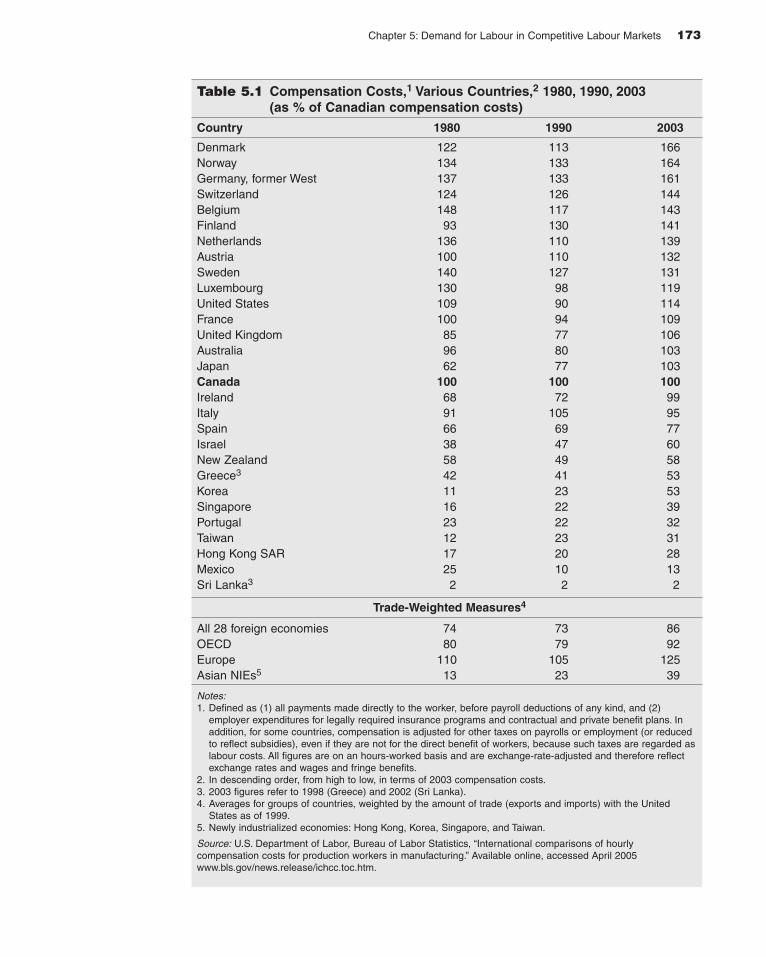
Table 5.1 compares compensation costs in Canada to a variety of countries throughoutthe world. The costs are converted to Canadian dollars on the basis of the exchange rate,and hence they reflect fluctuations in the exchange rate. They are specified on an hourlybasis so they are adjusted for differences in hours worked. The costs for each year areindexed to the Canadian costs, which are set equal to 100, so that they are all expressed aspercentages of the Canadian costs. For example, in 2003, compensation costs in thehighest-cost country, Denmark, were 166 percent of Canadian costs (i.e., 66 percent aboveCanadian costs), while the costs in the lowest-cost country of Mexico were 13 percent ofthose in Canada. The figures of Table 5.1 indicate that Canada is reasonably competitive onan international basis in terms of compensation costs. We are significantly below high-wage countries like Germany, Switzerland, the Netherlands, and the Scandinavian coun-tries, but significantly above low-wage countries like Mexico and the newly industrializedeconomies of Hong Kong, Korea, Singapore, and Taiwan (though the gap is narrowing).Canadian costs are also lower than those of our major trading partners the United Statesand Japan. An important point to bear in mind, however, is that one should not be entirelycheered by declining wages. From a welfare perspective, while low wages might make onemore competitive, they do not necessarily make one better off. National standards of liv-ing depend crucially on high wages derived from high productivity. This further empha-sizes the importance of considering productivity along with wage costs.

The continued success of higher wage countries like Germany and Japan shows the via-bility of being able to compete on the basis of productivity and quality, as opposed to low



Table 5.1 Compensation Costs,1 Various Countries,2 1980, 1990, 2003 (as % of Canadian compensation costs)

Country 1980 1990 2003

Denmark 122 113 166Norway 134 133 164Germany, former West 137 133 161Switzerland 124 126 144Belgium 148 117 143Finland 93 130 141Netherlands 136 110 139Austria 100 110 132Sweden 140 127 131Luxembourg 130 98 119United States 109 90 114France 100 94 109United Kingdom 85 77 106Australia 96 80 103Japan 62 77 103Canada 100 100 100Ireland 68 72 99Italy 91 105 95Spain 66 69 77Israel 38 47 60New Zealand 58 49 58Greece3 42 41 53Korea 11 23 53Singapore 16 22 39Portugal 23 22 32Taiwan 12 23 31Hong Kong SAR 17 20 28Mexico 25 10 13Sri Lanka3 2 2 2

Trade-Weighted Measures4

All 28 foreign economies 74 73 86OECD 80 79 92Europe 110 105 125Asian NIEs5 13 23 39

Notes:1. Defined as (1) all payments made directly to the worker, before payroll deductions of any kind, and (2)

employer expenditures for legally required insurance programs and contractual and private benefit plans. Inaddition, for some countries, compensation is adjusted for other taxes on payrolls or employment (or reducedto reflect subsidies), even if they are not for the direct benefit of workers, because such taxes are regarded aslabour costs. All figures are on an hours-worked basis and are exchange-rate-adjusted and therefore reflectexchange rates and wages and fringe benefits.

2. In descending order, from high to low, in terms of 2003 compensation costs.3. 2003 figures refer to 1998 (Greece) and 2002 (Sri Lanka).4. Averages for groups of countries, weighted by the amount of trade (exports and imports) with the United

States as of 1999.5. Newly industrialized economies: Hong Kong, Korea, Singapore, and Taiwan.

Source: U.S. Department of Labor, Bureau of Labor Statistics, “International comparisons of hourlycompensation costs for production workers in manufacturing.” Available online, accessed April 2005www.bls.gov/news.release/ichcc.toc.htm.

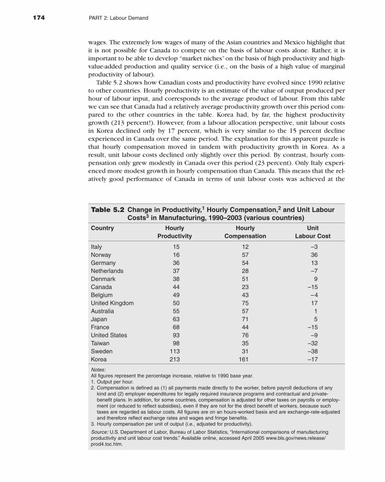
wages. The extremely low wages of many of the Asian countries and Mexico highlight thatit is not possible for Canada to compete on the basis of labour costs alone. Rather, it isimportant to be able to develop “market niches”on the basis of high productivity and high-value-added production and quality service (i.e., on the basis of a high value of marginalproductivity of labour).

Table 5.2 shows how Canadian costs and productivity have evolved since 1990 relativeto other countries. Hourly productivity is an estimate of the value of output produced perhour of labour input, and corresponds to the average product of labour. From this tablewe can see that Canada had a relatively average productivity growth over this period com-pared to the other countries in the table. Korea had, by far, the highest productivitygrowth (213 percent!). However, from a labour allocation perspective, unit labour costsin Korea declined only by 17 percent, which is very similar to the 15 percent declineexperienced in Canada over the same period. The explanation for this apparent puzzle isthat hourly compensation moved in tandem with productivity growth in Korea. As aresult, unit labour costs declined only slightly over this period. By contrast, hourly com-pensation only grew modestly in Canada over this period (23 percent). Only Italy experi-enced more modest growth in hourly compensation than Canada. This means that the rel-atively good performance of Canada in terms of unit labour costs was achieved at the


Table 5.2 Change in Productivity,1 Hourly Compensation,2 and Unit LabourCosts3 in Manufacturing, 1990–2003 (various countries)

Country Hourly Hourly UnitProductivity Compensation Labour Cost

Italy 15 12 –3Norway 16 57 36Germany 36 54 13Netherlands 37 28 –7Denmark 38 51 9Canada 44 23 –15Belgium 49 43 –4United Kingdom 50 75 17Australia 55 57 1Japan 63 71 5France 68 44 –15United States 93 76 –9Taiwan 98 35 –32Sweden 113 31 –38Korea 213 161 –17

Notes:All figures represent the percentage increase, relative to 1990 base year.1. Output per hour.2. Compensation is defined as (1) all payments made directly to the worker, before payroll deductions of any

kind and (2) employer expenditures for legally required insurance programs and contractual and private-benefit plans. In addition, for some countries, compensation is adjusted for other taxes on payrolls or employ-ment (or reduced to reflect subsidies), even if they are not for the direct benefit of workers, because suchtaxes are regarded as labour costs. All figures are on an hours-worked basis and are exchange-rate-adjustedand therefore reflect exchange rates and wages and fringe benefits.

3. Hourly compensation per unit of output (i.e., adjusted for productivity).

Source: U.S. Department of Labor, Bureau of Labor Statistics, “International comparisons of manufacturingproductivity and unit labour cost trends.” Available online, accessed April 2005 www.bls.gov/news.release/prod4.toc.htm.

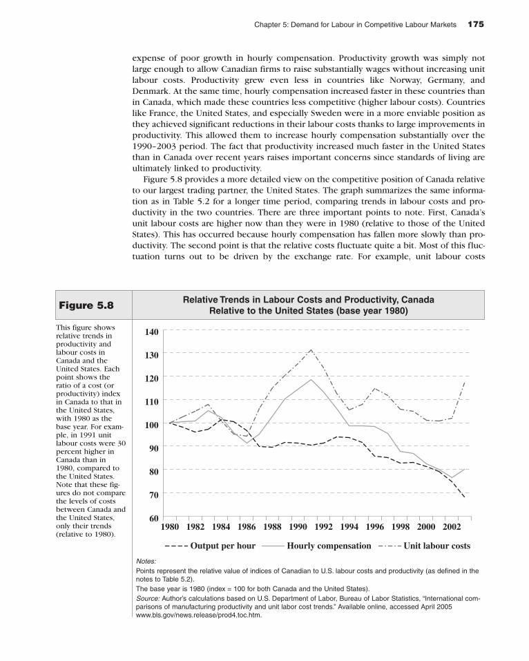
expense of poor growth in hourly compensation. Productivity growth was simply notlarge enough to allow Canadian firms to raise substantially wages without increasing unitlabour costs. Productivity grew even less in countries like Norway, Germany, andDenmark. At the same time, hourly compensation increased faster in these countries thanin Canada, which made these countries less competitive (higher labour costs). Countrieslike France, the United States, and especially Sweden were in a more enviable position asthey achieved significant reductions in their labour costs thanks to large improvements inproductivity. This allowed them to increase hourly compensation substantially over the1990–2003 period. The fact that productivity increased much faster in the United Statesthan in Canada over recent years raises important concerns since standards of living areultimately linked to productivity.

Figure 5.8 provides a more detailed view on the competitive position of Canada relativeto our largest trading partner, the United States. The graph summarizes the same informa-tion as in Table 5.2 for a longer time period, comparing trends in labour costs and pro-ductivity in the two countries. There are three important points to note. First, Canada’sunit labour costs are higher now than they were in 1980 (relative to those of the UnitedStates). This has occurred because hourly compensation has fallen more slowly than pro-ductivity. The second point is that the relative costs fluctuate quite a bit. Most of this fluc-tuation turns out to be driven by the exchange rate. For example, unit labour costs


60

70

80

90

100

110

120

130

140

Unit labour costsHourly compensationOutput per hour

200220001998199619941992199019881986198419821980

Figure 5.8

This figure showsrelative trends inproductivity andlabour costs inCanada and theUnited States. Eachpoint shows theratio of a cost (orproductivity) indexin Canada to that inthe United States,with 1980 as thebase year. For exam-ple, in 1991 unitlabour costs were 30percent higher inCanada than in1980, compared tothe United States.Note that these fig-ures do not comparethe levels of costsbetween Canada andthe United States,only their trends(relative to 1980).

Relative Trends in Labour Costs and Productivity, CanadaRelative to the United States (base year 1980)

Notes:Points represent the relative value of indices of Canadian to U.S. labour costs and productivity (as defined in thenotes to Table 5.2).The base year is 1980 (index = 100 for both Canada and the United States).Source: Author’s calculations based on U.S. Department of Labor, Bureau of Labor Statistics, “International com-parisons of manufacturing productivity and unit labor cost trends.” Available online, accessed April 2005www.bls.gov/news.release/prod4.toc.htm.

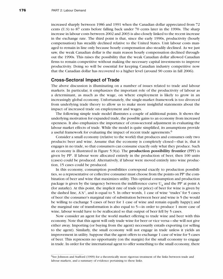
increased sharply between 1986 and 1991 when the Canadian dollar appreciated from 72cents (U.S) to 87 cents before falling back under 70 cents later in the 1990s. The sharpincrease in labour costs between 2002 and 2003 is also closely linked to the recent increasein the exchange rate. The third point is that, since the early 1990s, productivity (hourlycompensation) has steadily declined relative to the United States. Unit labour costs man-aged to remain in line only because hourly compensation also steadily declined. As we justsaw, the weak Canadian dollar is the main reason hourly compensation declined through-out the 1990s. This raises the possibility that the weak Canadian dollar allowed Canadianfirms to remain competitive without making the necessary capital investments to improveproductivity. Doing so will be essential for keeping Canadian industry competitive nowthat the Canadian dollar has recovered to a higher level (around 90 cents in fall 2006).

Cross-Sectoral Impact of TradeThe above discussion is illuminating on a number of issues related to trade and labourmarkets. In particular, it emphasizes the important role of the productivity of labour as a determinant, as much as the wage, on where employment is likely to grow in anincreasingly global economy. Unfortunately, the single-market framework is too divorcedfrom underlying trade theory to allow us to make more insightful statements about theimpact of increased trade on employment and wages.

The following simple trade model illustrates a couple of additional points. It shows theunderlying motivation for expanded trade, the possible gains to an economy from increasedopenness. It also emphasizes the importance of cross-sectoral adjustment in evaluating thelabour market effects of trade. While the model is quite simplified, its assumptions providea useful framework for evaluating the impact of recent trade agreements.6

Consider a small economy (relative to the world) that produces and consumes only twoproducts: beer and wine. Assume that the economy is completely closed—that is, that itengages in no trade, so that consumers can consume exactly only what they produce. Suchan economy is illustrated in Figure 5.9(a). The production possibility frontier (PPF) isgiven by PP'. If labour were allocated entirely in the production of beer, then 100 units(cases) could be produced. Alternatively, if labour were moved entirely into wine produc-tion, 15 cases could be produced.

In this economy, consumption possibilities correspond exactly to production possibili-ties, so a representative or collective consumer must choose from the points on PP' the com-bination of beer and wine that maximizes utility. This optimal consumption and productionpackage is given by the tangency between the indifference curve UA and the PP' at point A(for autarky). At this point, the implicit rate of trade (or price) of beer for wine is given bythe dashed line, A'A'', and is equal to 5. In other words, 1 case of wine “trades” for 5 casesof beer: the consumer’s marginal rate of substitution between beer and wine is 5 (he wouldbe willing to exchange 5 cases of beer for 1 case of wine and remain equally happy); andthe marginal rate of transformation is also equal to 5—in order to produce 1 more case ofwine, labour would have to be reallocated so that output of beer fell by 5 cases.

Now consider an agent for the world market offering to trade wine and beer with thiseconomy. Note that this agent will only trade wine for beer or vice versa—she will not giveeither away. Importing (or buying from the agent) necessarily entails exporting (or sellingto the agent). Similarly, the small economy will not engage in trade unless it yields animprovement in utility. Suppose that the agent offers to exchange 1 case of wine for 5 casesof beer. This represents no opportunity (on the margin) for the small economy to engagein trade. In order for the international agent to offer something to the small economy, there


6See Johnson and Stafford (1999) for a theoretically more rigorous treatment of the links between trade andlabour markets, and a summary of evidence pertaining to these links.

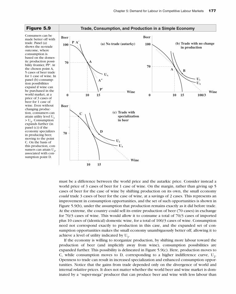
must be a difference between the world price and the autarkic price. Consider instead aworld price of 3 cases of beer for 1 case of wine. On the margin, rather than giving up 5cases of beer for the case of wine by shifting production on its own, the small economycould trade 3 cases of beer for the case of wine, at a savings of 2 cases. This represents animprovement in consumption opportunities, and the set of such opportunities is shown inFigure 5.9(b), under the assumption that production remains exactly as it did before trade.At the extreme, the country could sell its entire production of beer (70 cases) in exchangefor 70/3 cases of wine. This would allow it to consume a total of 70/3 cases of importedplus 10 cases of (identical) domestic wine, for a total of 100/3 cases of wine. Consumptionneed not correspond exactly to production in this case, and the expanded set of con-sumption opportunities makes the small economy unambiguously better off, allowing it toachieve a level of utility indicated by U1.

If the economy is willing to reorganize production, by shifting more labour toward theproduction of beer (and implicitly away from wine), consumption possibilities areexpanded further. This possibility is delineated in Figure 5.9(c). Here, production moves toC, while consumption moves to D, corresponding to a higher indifference curve, U2.Openness to trade can result in increased specialization and enhanced consumption oppor-tunities. Notice that the gains from trade depended only on the divergence of world andinternal relative prices. It does not matter whether the world beer and wine market is dom-inated by a “super-mega” producer that can produce beer and wine with less labour than


100

70

A″

UA

A′

A

P′

BeerP (a) No trade (autarky) (b) Trade with no change

in production

(c) Trade with specialization in beer

100

100

70BA

U1

UA

100 15

Beer

15Wine Wine

10 15Wine

UA

U2

D

C•

••

•

Beer

••70

100/3

Figure 5.9Consumers can bemade better off withtrade. Panel (a)shows the no-tradeoutcome, whereconsumption isbased on the domes-tic production possi-bility frontier, PP'. Atthe chosen point A,5 cases of beer tradefor 1 case of wine. Inpanel (b) consump-tion possibilitiesexpand if wine canbe purchased in theworld market, at aprice of 3 cases ofbeer for 1 case ofwine. Even withoutchanging produc-tion, consumers canattain utility level U1> UA. Consumptionexpands further (inpanel (c)) if theeconomy specializesin producing beer,moving to the pointC. On the basis ofthis production, con-sumers can attain U2,associated with con-sumption point D.

Trade, Consumption, and Production in a Simple Economy

the small economy, or an inefficient producer of both goods. All that matters is the differ-ence in the relative productivity in production of beer and wine. This is the basic notion ofcomparative advantage, the driving force in the theoretical arguments regarding the gainsfrom trade.

This simple model illustrates why most economists favour free trade as a general prin-ciple. Consumers are made unambiguously better off with increased opportunities totrade. The value of the model also lies in its ability to assess the likely impact of increasedtrade on the labour market. First, it suggests that trade leads to sectoral adjustment— somesectors will expand, while others will shrink. Unless the world economy is “giving away”its output, at least one sector must expand in order for the small economy to be able topurchase the world-produced goods. Looking at aggregate employment statistics may nottell the full story of the effects of trade on the labour market. Second, the argument for thegains from trade assumes that there is a representative consumer, or equivalently, that theconsumption pie is shared equally with all members of the small economy. If the labourallocated in the shrinking sector does not share in the increased consumption opportuni-ties, then the argument that trade is necessarily welfare-enhancing is questionable. In morepractical terms, unless the “losers” are compensated, or costlessly shifted to the “winning”sector, it is not necessarily the case that freer trade makes the small economy better off.We will be pursuing these issues further in our examination of inequality and wage differ-entials, later in Chapter 9.

EvidenceWith these theoretical insights behind us, let us turn to the more specific question of howfreer trade has affected the Canadian labour market, especially since the Canada–U.S. freetrade agreement (FTA) was implemented in 1989. The effects were expected to be posi-tive: job gains exceeding job losses, increases in real wages, and reductions in unemploy-ment. However, more than 15 years after its beginning, controversy remains about itsactual effects, with opponents attributing mass layoffs and plant closings to the FTA. It hasbeen difficult to isolate the independent impact of the FTA, in part because it was phasedin over a ten-year period, but more importantly because it was only one of many interre-lated forces affecting the labour market at the time (Betcherman and Gunderson, 1990).The other forces include those discussed in this section—global competition, industrialstructuring, technological change, privatization, and subcontracting. The FTA also coin-cided with a recession in both Canada and the United States, and a high Canadian dollar(recall Figure 5.8).

An increasing consensus is emerging about the overall impact of the FTA. First, therewere definite short-run adjustment costs, especially in heavily protected industries, that is,those that had the largest tariff reductions. Gaston and Trefler (1997) estimate that of the400,000 jobs lost in Canada between 1989 and 1993, between 9 and 14 percent (around40,000 jobs) can be attributed to the FTA, netting out the variety of other contributingfactors. To some extent, both Gaston and Trefler and a more recent study by Beaulieu(2000) attribute the adjustment costs to inflexibility (wage rigidity) in the Canadian labourmarket. Implicit in our discussion of the gains from trade is a costless reallocation of labourfrom the shrinking sector to the expanding one. If this reallocation is impeded by labourmarket imperfections, the potentially adverse consequences of trade are magnified. Gastonand Trefler’s results emphasize the importance of labour market structure in assessing thebenefits of freer trade.

However, Trefler (2001) also shows that while the short-run costs are evident, there havealso been significant long-run benefits of the FTA, especially in terms of higher labour pro-ductivity. The reallocation of labour out of the less productive into the more productiveplants has led to increases in labour productivity of 0.6 percent per year in all of manufac-


turing, and a “staggering” 2.1-percent-per-year increase in those manufacturing industriesmost affected by free trade. While painful in the short run, the specialization in more pro-ductive activities (or modes of production) generates long-run benefits, largely in line withwhat we would expect using the simple trade models, such as those discussed in Figure 5.9.

Other Demand-Side FactorsAs noted previously, there have been a number of other important changes occurring onthe demand side of the Canadian labour market. Industrial restructuring has also beenprominent, associated mainly with the decline of blue-collar, often unionized, well-paidjobs in heavy manufacturing. As outlined in more detail later in the chapter on wage struc-tures, these middle-wage jobs have been displaced by jobs at polar ends of the occupa-tional distribution. At the high end are professional, managerial, and administrative jobs; atthe low end are the low-wage jobs in services and retailing. This phenomenon has beendescribed as the “declining middle” and it has led to increased wage polarization.


In 1990 and 1991, opponents of free trade linked the Canada–U.S. free tradeagreement to the significant job loss experienced in Canada over this time period.Hardly a day went by without the media reporting of one factory or another clos-ing down and moving to the United States. While employment has recovered sig-nificantly since that time, to what extent were FTA opponents correct in layingblame on free trade for these job losses? As it turns out, this is a difficult questionto answer. The job losses at the time coincided with four other major adverse eco-nomic factors: (1) a severe recession that occurred in both Canada and the UnitedStates; (2) a high Canadian dollar, the increased value of which may have offsetany favourable effects of U.S. tariff reductions (recall Figure 5.8); (3) high relativeCanadian interest rates, which may have contributed to higher relative economiccontraction; and (4) ongoing structural adjustment, and other manifestations oftechnological change and globalization.

Gaston and Trefler (1994, 1997) present a thorough and careful attempt to dis-entangle these factors. Given lags in data availability, their studies focus onchanges up to 1993, corresponding to the depths of the last recession. They pointout that any “conviction” of the FTA for job destruction depends on establishing alink between job loss and trade, and furthermore, to the tariff changes that couldbe associated with changed trade patterns. The aggregate employment condi-tions at the time cannot be blamed on the FTA, or at least FTA proponents canreasonably argue that other factors might have been responsible. Thus, theGaston and Trefler studies look at cross-industry variation in employment growth,compared across the two countries.

They show that employment decline, especially in “sunset” or declining indus-tries, was more severe in Canada. This could be associated with changed tariffs.However, some of the more severe employment declines occurred in industriesthat were less affected by the FTA (automobiles, steel, and lumber for example).In the end, they attribute only about 9 to 14 percent of the overall job loss (around400,000 jobs) to tariff changes resulting from the FTA. Furthermore, they point outthat some of this loss would have been reduced if Canadian wages had adjustedmore toward the U.S. level.

Free Trade and JobsExhibit 5.2

The large factories of the heavy-manufacturing, “smokestack” industries have oftengiven way to more flexible, modular factories linked together by advanced communica-tions and “just in time” delivery systems that require little inventory. Flexibility and adapt-ability are crucial, and the need for these elements has led to increases in subcontracting,permanent part-time work forces, and contingent work forces that are utilized as demandchanges. The industrial restructuring has often been accompanied through mergers andacquisitions, often leading to work force reductions (“downsizing”) and pressures forconcession bargaining.

Technological change has continued its advance, especially in areas of information andcommunication technologies (ICTs). These technologies and the Internet have dramati-cally reshaped the internal organization of firms and business practices. Robotics has beenintroduced on the factory floor and the assembly line, and computer-assisted technologyhas been utilized in virtually every aspect of the production cycle.

In the public sector, privatization and subcontracting have been prominent for func-tions ranging from building maintenance to road maintenance. Former Crown corpora-tions such as Air Canada have also been privatized.

These various changes emanating from the demand side of the labour market have sig-nificant implications both for labour markets and for human resource practices and indus-trial relations policies in general. They imply greater demands for a flexible and adaptablework force, just like the flexibility that is required from the product market side fromwhich the demand for labour is derived. The work force must be willing and able to do abroader array of job assignments and to integrate quality control as an integral part of thejob. The product market changes place greater emphasis on a work force that is trained inthe general skills required for continuous upgrading and retraining and is also able to do avariety of tasks (“multiskilling”) associated with the broader job assignments and theemphasis on quality control. As part of the individual worker’s responsibility for qualitycontrol, there is less emphasis on direct supervision and more emphasis on employeeinvolvement in decision-making.

The demand-side changes are also pressuring for compensation that is more flexible andresponsive to the changing economic conditions and to the particular economic circum-stances of each individual enterprise. This in turn puts pressure toward the breakdown ofhistorical pattern bargaining that often prevailed, whereby establishments frequently fol-lowed the wage settlements established by certain key pattern-setting firms. This may nolonger be viable given the different demand conditions facing different firms.

The changes emanating from the demand side of the labour market have also led tonumerous changes in workplace practices. Jobs have often been redesigned to provide forboth job enlargement (the horizontal addition of a variety of tasks of similar complexity)and job enrichment (the vertical addition of tasks of different levels of complexity).

Whether these changes are part of a fundamental transformation or a continuous evo-lution of the workplace and the labour market is a debatable issue. What is certain is thatthe demand-side forces are having a substantial impact. The impact is particularly pro-nounced because the forces tend to work in the same direction, thereby compoundingtheir individual effects. When coupled with many of the supply-side pressures highlightedpreviously (aging work force, continued labour force participation of women, dominanceof the two-earner family), they emphasize the dynamism that will continue to characterizethe Canadian labour market.


Summary


• Labour demand is “derived demand,” that is, labouris hired in order to produce goods that are sold inthe product market. For this reason, labourdemand is always connected to the product mar-ket, especially in terms of the degree of competi-tion, whether from foreign or domestic producers.

• Labour is only one of several factors of production.In the short run, we imagine that all of these otherfactors are fixed, and labour is the only variableinput. The profit-maximizing level of labourdemand will be chosen so that the marginal bene-fit equals the marginal cost of hiring an additionalunit of labour. The marginal cost is the wage rate,while the marginal benefit is the revenue associ-ated with the extra production by that worker, itsmarginal revenue product (MRPN ). Therefore, theshort-run labour demand function is given by theMRPN schedule, where employment is determinedby W = MRPN.

• In the long run, labour can be substituted withother inputs like capital. An increase in the wagewill have two effects on the quantity of labourdemanded. First, even if output remains the same,

the firm will substitute toward capital and awayfrom labour (the substitution effect). Second, theincrease in marginal cost will lead to a reduction inthe optimal output, and a further reduction inlabour demanded (the scale effect).

• Labour demand curves unambiguously slopedownward, in both the long and short run. Thelong-run function is more elastic (at any givenwage), because of the greater degree of flexibilityin substituting other inputs for labour.

• The impact of globalization and outsourcing on theCanadian labour market can be analyzed in thecontext of a simple labour demand model, whereemployment in Canada depends on labour produc-tivity and labour costs in Canada versus the rest ofthe world. However, a richer model allowing formore than a single sector provides a better under-standing of the cross-sectoral impacts of increasedtrade on employment, wages, and economic wel-fare, and also highlights the important role playedby comparative advantage in determining tradeand employment patterns.

KEYWORDS

complements 172cost minimization 156derived demand 151diminishing marginal returns

154elasticity of demand for labour

166factor of production 151fixed costs 153ICTs 170isocost line 158

isoquant 157long run 151Maquiladora 170marginal cost 153marginal physical product 155marginal rate of technical

substitution 157marginal revenue 153marginal revenue product 154monopolist 153outsourcing 170

production function 153production possibility frontier

(PPF) 176productivity 172profit maximization 153scale effect 160short run 151total revenue product 154value of the marginal product

155variable costs 153

REVIEW QUESTIONS

1. Why is the point E0 in Figure 5.2(c) a stable equi-librium? Show the firm’s expansion path. That is,show how the firm’s input mix evolves as output isincreased.

2. What is meant by an inferior factor of production?How would the firm’s demand for labour be alteredif labour were an inferior factor of production?

3. “The firm’s demand schedule for labour is a nega-tive function of the wage because, as the firm usesmore labour, it has to utilize poorer-quality labour,and hence pays a lower wage.” True or false?Explain.

4. Derive the firm’s demand schedule for labour if itwere a monopolist that could influence the price

www.mcgrawhill.ca/olc/benjamin

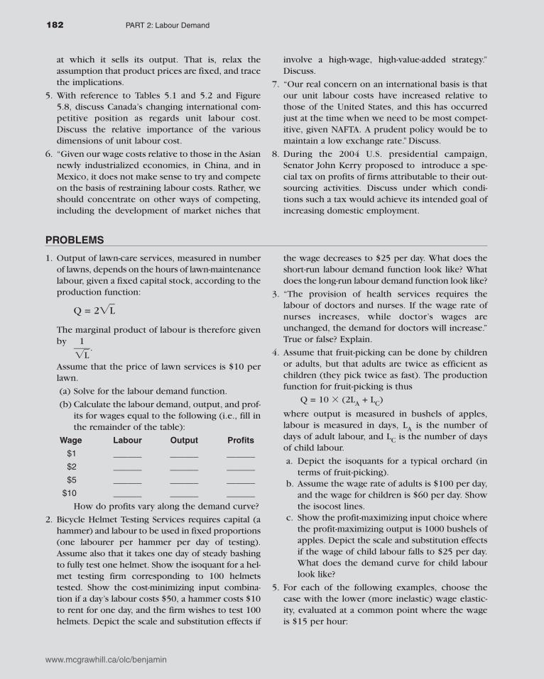
at which it sells its output. That is, relax theassumption that product prices are fixed, and tracethe implications.

5. With reference to Tables 5.1 and 5.2 and Figure5.8, discuss Canada’s changing international com-petitive position as regards unit labour cost.Discuss the relative importance of the variousdimensions of unit labour cost.

6. “Given our wage costs relative to those in the Asiannewly industrialized economies, in China, and inMexico, it does not make sense to try and competeon the basis of restraining labour costs. Rather, weshould concentrate on other ways of competing,including the development of market niches that

involve a high-wage, high-value-added strategy.”Discuss.

7. “Our real concern on an international basis is thatour unit labour costs have increased relative tothose of the United States, and this has occurredjust at the time when we need to be most compet-itive, given NAFTA. A prudent policy would be tomaintain a low exchange rate.” Discuss.

8. During the 2004 U.S. presidential campaign,Senator John Kerry proposed to introduce a spe-cial tax on profits of firms attributable to their out-sourcing activities. Discuss under which condi-tions such a tax would achieve its intended goal ofincreasing domestic employment.


PROBLEMS

1. Output of lawn-care services, measured in numberof lawns, depends on the hours of lawn-maintenancelabour, given a fixed capital stock, according to theproduction function:

Q = 2�L�

The marginal product of labour is therefore givenby

��1

L��.

Assume that the price of lawn services is $10 perlawn.

(a) Solve for the labour demand function.

(b) Calculate the labour demand, output, and prof-its for wages equal to the following (i.e., fill inthe remainder of the table):

Wage Labour Output Profits

$1 ______ ______ ______

$2 ______ ______ ______

$5 ______ ______ ______

$10 ______ ______ ______

How do profits vary along the demand curve?

2. Bicycle Helmet Testing Services requires capital (ahammer) and labour to be used in fixed proportions(one labourer per hammer per day of testing).Assume also that it takes one day of steady bashingto fully test one helmet. Show the isoquant for a hel-met testing firm corresponding to 100 helmetstested. Show the cost-minimizing input combina-tion if a day’s labour costs $50, a hammer costs $10to rent for one day, and the firm wishes to test 100helmets. Depict the scale and substitution effects if

the wage decreases to $25 per day. What does theshort-run labour demand function look like? Whatdoes the long-run labour demand function look like?

3. “The provision of health services requires thelabour of doctors and nurses. If the wage rate ofnurses increases, while doctor’s wages areunchanged, the demand for doctors will increase.”True or false? Explain.

4. Assume that fruit-picking can be done by childrenor adults, but that adults are twice as efficient aschildren (they pick twice as fast). The productionfunction for fruit-picking is thus

Q = 10 � (2LA + LC)

where output is measured in bushels of apples,labour is measured in days, LA is the number ofdays of adult labour, and LC is the number of daysof child labour.

a. Depict the isoquants for a typical orchard (interms of fruit-picking).

b. Assume the wage rate of adults is $100 per day,and the wage for children is $60 per day. Showthe isocost lines.

c. Show the profit-maximizing input choice wherethe profit-maximizing output is 1000 bushels ofapples. Depict the scale and substitution effectsif the wage of child labour falls to $25 per day.What does the demand curve for child labourlook like?

5. For each of the following examples, choose thecase with the lower (more inelastic) wage elastic-ity, evaluated at a common point where the wageis $15 per hour:


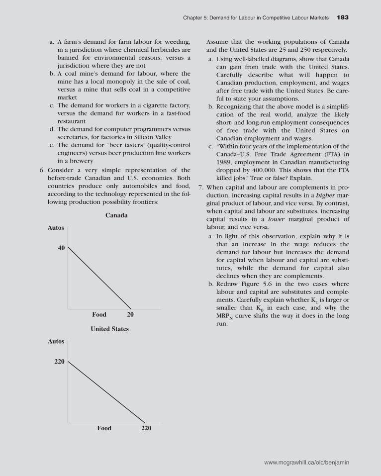
a. A farm’s demand for farm labour for weeding,in a jurisdiction where chemical herbicides arebanned for environmental reasons, versus ajurisdiction where they are not

b. A coal mine’s demand for labour, where themine has a local monopoly in the sale of coal,versus a mine that sells coal in a competitivemarket

c. The demand for workers in a cigarette factory,versus the demand for workers in a fast-foodrestaurant

d. The demand for computer programmers versussecretaries, for factories in Silicon Valley

e. The demand for “beer tasters” (quality-controlengineers) versus beer production line workersin a brewery

6. Consider a very simple representation of thebefore-trade Canadian and U.S. economies. Bothcountries produce only automobiles and food,according to the technology represented in the fol-lowing production possibility frontiers:

Assume that the working populations of Canadaand the United States are 25 and 250 respectively.

a. Using well-labelled diagrams, show that Canadacan gain from trade with the United States.Carefully describe what will happen toCanadian production, employment, and wagesafter free trade with the United States. Be care-ful to state your assumptions.

b. Recognizing that the above model is a simplifi-cation of the real world, analyze the likelyshort- and long-run employment consequencesof free trade with the United States onCanadian employment and wages.

c. “Within four years of the implementation of theCanada–U.S. Free Trade Agreement (FTA) in1989, employment in Canadian manufacturingdropped by 400,000. This shows that the FTAkilled jobs.” True or false? Explain.

7. When capital and labour are complements in pro-duction, increasing capital results in a higher mar-ginal product of labour, and vice versa. By contrast,when capital and labour are substitutes, increasingcapital results in a lower marginal product oflabour, and vice versa.

a. In light of this observation, explain why it isthat an increase in the wage reduces thedemand for labour but increases the demandfor capital when labour and capital are substi-tutes, while the demand for capital alsodeclines when they are complements.

b. Redraw Figure 5.6 in the two cases wherelabour and capital are substitutes and comple-ments. Carefully explain whether K1 is larger orsmaller than K0 in each case, and why theMRPN curve shifts the way it does in the longrun.


United States

Autos

220

220

Food

Canada

Food

Autos

20

40
