NUMERICAL METHODS FOR PARTIAL DIFFERENTIAL EQUATIONS http://pde.fusion.kth.se Andr´ e Jaun <[email protected]> September 10, 2001 with the participation of Thomas Johnson <[email protected]> Thomas H¨ urtig <[email protected]> Thomas Rylander <[email protected]> Mikael Persson <[email protected]> Laurent Villard <Laurent.Villard@epfl.ch> Amplitude Position -32 32 Zabuski’s finite difference scheme for solitons 1 0 2001 course of the Summer University of Southern Stockholm, held simultaneously at the Ecole Polytechnique F´ ed´ erale de Lausanne, Lausanne, Switzerland Chalmers Institute of Technology, G¨oteborg, Sweden Royal Institute of Technology, Stockholm, Sweden

Welcome message from author
This document is posted to help you gain knowledge. Please leave a comment to let me know what you think about it! Share it to your friends and learn new things together.
Transcript
NUMERICAL METHODS FOR PARTIAL
DIFFERENTIAL EQUATIONS
http://pde.fusion.kth.se
Andre Jaun <[email protected]>
September 10, 2001
with the participation of
Thomas Johnson <[email protected]>Thomas Hurtig <[email protected]>
Thomas Rylander <[email protected]>Mikael Persson <[email protected]>Laurent Villard <[email protected]>
Am
plit
ud
e
Position-32 32
Zabuski’s finite difference scheme for solitons1
0
2001 course of the Summer University of Southern Stockholm, held simultaneously at theEcole Polytechnique Federale de Lausanne, Lausanne, Switzerland
Chalmers Institute of Technology, Goteborg, SwedenRoyal Institute of Technology, Stockholm, Sweden

ii
This document is typeset with LATEX 2ε1 using the macros in the latex2html2 packageon Sun3 and Linux4 platforms.
c© A. Jaun, J. Hedin, T. Johnson, 1999-2001, TRITA-ALF-1999-05 report, Royal Instituteof Technology, Stockholm, Sweden.
1http://www.tug.org/2http://cdc-server.cdc.informatik.tu-darmstadt.de/%7Elatex2html3http://www.sun.com4http://www.linux.org
CONTENTS iii
Contents
1 INTRODUCTION 51.1 How to study this course . . . . . . . . . . . . . . . . . . . . . . . . . . . . . 51.2 Differential Equations . . . . . . . . . . . . . . . . . . . . . . . . . . . . . . 7
1.2.1 Ordinary differential equations . . . . . . . . . . . . . . . . . . . . . 71.2.2 Partial differential equations . . . . . . . . . . . . . . . . . . . . . . 81.2.3 Boundary / initial conditions . . . . . . . . . . . . . . . . . . . . . . 81.2.4 Characteristics and dispersion relations . . . . . . . . . . . . . . . . 91.2.5 Moments & conservation laws . . . . . . . . . . . . . . . . . . . . . . 9
1.3 Prototype problems . . . . . . . . . . . . . . . . . . . . . . . . . . . . . . . 101.3.1 Advection . . . . . . . . . . . . . . . . . . . . . . . . . . . . . . . . . 101.3.2 Diffusion . . . . . . . . . . . . . . . . . . . . . . . . . . . . . . . . . 101.3.3 Dispersion . . . . . . . . . . . . . . . . . . . . . . . . . . . . . . . . . 111.3.4 Wave-breaking . . . . . . . . . . . . . . . . . . . . . . . . . . . . . . 111.3.5 Schrodinger . . . . . . . . . . . . . . . . . . . . . . . . . . . . . . . . 12
1.4 Discretization . . . . . . . . . . . . . . . . . . . . . . . . . . . . . . . . . . . 121.4.1 Convergence . . . . . . . . . . . . . . . . . . . . . . . . . . . . . . . 131.4.2 Sampling on a grid . . . . . . . . . . . . . . . . . . . . . . . . . . . . 131.4.3 Finite elements . . . . . . . . . . . . . . . . . . . . . . . . . . . . . . 141.4.4 Splines . . . . . . . . . . . . . . . . . . . . . . . . . . . . . . . . . . . 141.4.5 Harmonic functions . . . . . . . . . . . . . . . . . . . . . . . . . . . 161.4.6 Wavelets . . . . . . . . . . . . . . . . . . . . . . . . . . . . . . . . . . 161.4.7 Quasi-particles . . . . . . . . . . . . . . . . . . . . . . . . . . . . . . 19
1.5 Exercises . . . . . . . . . . . . . . . . . . . . . . . . . . . . . . . . . . . . . 211.0 E-publishing . . . . . . . . . . . . . . . . . . . . . . . . . . . . . . . 211.1 Stiff ODE . . . . . . . . . . . . . . . . . . . . . . . . . . . . . . . . . 211.2 Predator-Prey model . . . . . . . . . . . . . . . . . . . . . . . . . . . 211.3 Fourier-Laplace transform . . . . . . . . . . . . . . . . . . . . . . . . 211.4 Random-walk . . . . . . . . . . . . . . . . . . . . . . . . . . . . . . . 211.5 Convergence . . . . . . . . . . . . . . . . . . . . . . . . . . . . . . . 221.6 Laplacian in 2D . . . . . . . . . . . . . . . . . . . . . . . . . . . . . 221.7 Hypercube . . . . . . . . . . . . . . . . . . . . . . . . . . . . . . . . 22
1.6 Further reading . . . . . . . . . . . . . . . . . . . . . . . . . . . . . . . . . . 221.7 Solutions . . . . . . . . . . . . . . . . . . . . . . . . . . . . . . . . . . . . . 231.8 Interactive evaluation form . . . . . . . . . . . . . . . . . . . . . . . . . . . 25
2 FINITE DIFFERENCES 272.1 Explicit 2 levels . . . . . . . . . . . . . . . . . . . . . . . . . . . . . . . . . . 272.2 Explicit 3 levels . . . . . . . . . . . . . . . . . . . . . . . . . . . . . . . . . . 292.3 Lax-Wendroff . . . . . . . . . . . . . . . . . . . . . . . . . . . . . . . . . . . 292.4 Leapfrog, staggered grid . . . . . . . . . . . . . . . . . . . . . . . . . . . . . 302.5 Implicit Crank-Nicholson . . . . . . . . . . . . . . . . . . . . . . . . . . . . 31
2.5.1 Advection-diffusion equation . . . . . . . . . . . . . . . . . . . . . . 312.5.2 Schrodinger equation . . . . . . . . . . . . . . . . . . . . . . . . . . . 33
2.6 Exercises . . . . . . . . . . . . . . . . . . . . . . . . . . . . . . . . . . . . . 342.1 Upwind differences, boundary conditions . . . . . . . . . . . . . . . . 342.2 Numerical dispersion . . . . . . . . . . . . . . . . . . . . . . . . . . . 35
iv CONTENTS
2.3 Shock waves using Lax-Wendroff . . . . . . . . . . . . . . . . . . . . 352.4 Leapfrog resonator . . . . . . . . . . . . . . . . . . . . . . . . . . . . 352.5 European option . . . . . . . . . . . . . . . . . . . . . . . . . . . . . 352.6 Particle in a periodic potential . . . . . . . . . . . . . . . . . . . . . 36
2.7 Further Reading . . . . . . . . . . . . . . . . . . . . . . . . . . . . . . . . . 362.8 Solutions . . . . . . . . . . . . . . . . . . . . . . . . . . . . . . . . . . . . . 362.9 Interactive evaluation form . . . . . . . . . . . . . . . . . . . . . . . . . . . 39
3 FINITE ELEMENTS METHODS 413.1 Mathematical background . . . . . . . . . . . . . . . . . . . . . . . . . . . . 413.2 An engineer’s formulation . . . . . . . . . . . . . . . . . . . . . . . . . . . . 423.3 Numerical quadrature and solution . . . . . . . . . . . . . . . . . . . . . . . 433.4 Linear solvers . . . . . . . . . . . . . . . . . . . . . . . . . . . . . . . . . . . 463.5 Variational inequalities . . . . . . . . . . . . . . . . . . . . . . . . . . . . . . 483.6 Exercises . . . . . . . . . . . . . . . . . . . . . . . . . . . . . . . . . . . . . 49
3.1 Quadrature . . . . . . . . . . . . . . . . . . . . . . . . . . . . . . . . 493.2 Diffusion in a cylinder . . . . . . . . . . . . . . . . . . . . . . . . . . 493.3 Mass lumping . . . . . . . . . . . . . . . . . . . . . . . . . . . . . . . 503.4 Iterative solver . . . . . . . . . . . . . . . . . . . . . . . . . . . . . . 503.5 Obstacle problem . . . . . . . . . . . . . . . . . . . . . . . . . . . . . 503.6 Numerical dispersion . . . . . . . . . . . . . . . . . . . . . . . . . . . 503.7 American option . . . . . . . . . . . . . . . . . . . . . . . . . . . . . 50
3.7 Further reading . . . . . . . . . . . . . . . . . . . . . . . . . . . . . . . . . . 513.8 Interactive evaluation form . . . . . . . . . . . . . . . . . . . . . . . . . . . 51
4 FOURIER TRANSFORM 534.1 Fast Fourier Transform (FFT) with the computer . . . . . . . . . . . . . . . 534.2 Linear equations. . . . . . . . . . . . . . . . . . . . . . . . . . . . . . . . . . 544.3 Aliasing, filters and convolution. . . . . . . . . . . . . . . . . . . . . . . . . 554.4 Non-linear equations. . . . . . . . . . . . . . . . . . . . . . . . . . . . . . . . 574.5 Exercises . . . . . . . . . . . . . . . . . . . . . . . . . . . . . . . . . . . . . 59
4.1 Advection-diffusion . . . . . . . . . . . . . . . . . . . . . . . . . . . . 594.2 Equivalent filter for Zabusky’s FD scheme . . . . . . . . . . . . . . . 594.3 Prototype problems . . . . . . . . . . . . . . . . . . . . . . . . . . . 604.4 Intrinsic numerical diffusion . . . . . . . . . . . . . . . . . . . . . . . 60
4.6 Further Reading . . . . . . . . . . . . . . . . . . . . . . . . . . . . . . . . . 604.7 Interactive evaluation form . . . . . . . . . . . . . . . . . . . . . . . . . . . 60
5 MONTE-CARLO METHODS 615.1 Monte Carlo integration . . . . . . . . . . . . . . . . . . . . . . . . . . . . . 615.2 Stochastic theory . . . . . . . . . . . . . . . . . . . . . . . . . . . . . . . . . 615.3 Particle orbits . . . . . . . . . . . . . . . . . . . . . . . . . . . . . . . . . . . 625.4 A scheme for the advection diffusion equation . . . . . . . . . . . . . . . . . 645.5 When should you use Monte Carlo methods? . . . . . . . . . . . . . . . . . 665.6 Exercises . . . . . . . . . . . . . . . . . . . . . . . . . . . . . . . . . . . . . 66
5.1 Expectancy and variance . . . . . . . . . . . . . . . . . . . . . . . . 665.2 Diffusion statistics . . . . . . . . . . . . . . . . . . . . . . . . . . . . 675.3 Periodic boundary conditions . . . . . . . . . . . . . . . . . . . . . . 67
CONTENTS 1
5.4 Steady state with velocity gradient . . . . . . . . . . . . . . . . . . . 675.5 Diffusion coefficient gradient . . . . . . . . . . . . . . . . . . . . . . 685.6 Evolution of a crowd of people . . . . . . . . . . . . . . . . . . . . . 68
5.7 Further readings . . . . . . . . . . . . . . . . . . . . . . . . . . . . . . . . . 685.8 Interactive evaluation form . . . . . . . . . . . . . . . . . . . . . . . . . . . 69
6 LAGRANGIAN METHODS 716.1 Introduction . . . . . . . . . . . . . . . . . . . . . . . . . . . . . . . . . . . . 716.2 Cubic-Interpolated Propagation (CIP) . . . . . . . . . . . . . . . . . . . . . 716.3 Non-Linear equations with CIP . . . . . . . . . . . . . . . . . . . . . . . . . 726.4 Exercises . . . . . . . . . . . . . . . . . . . . . . . . . . . . . . . . . . . . . 73
6.1 Arbitrary CFL number . . . . . . . . . . . . . . . . . . . . . . . . . 736.2 Diffusion in CIP . . . . . . . . . . . . . . . . . . . . . . . . . . . . . 736.3 Lagrangian method with splines . . . . . . . . . . . . . . . . . . . . 736.4 Non-linear equation . . . . . . . . . . . . . . . . . . . . . . . . . . . 73
6.5 Further Reading . . . . . . . . . . . . . . . . . . . . . . . . . . . . . . . . . 736.6 Interactive evaluation form . . . . . . . . . . . . . . . . . . . . . . . . . . . 73
7 WAVELETS 757.1 Remain a matter of research . . . . . . . . . . . . . . . . . . . . . . . . . . . 75
8 THE JBONE USER MANUAL 798.1 Source code & installation . . . . . . . . . . . . . . . . . . . . . . . . . . . . 798.2 Program execution . . . . . . . . . . . . . . . . . . . . . . . . . . . . . . . . 808.3 Program structure & documentation . . . . . . . . . . . . . . . . . . . . . . 818.4 An object-oriented example: Monte-Carlo in JBONE . . . . . . . . . . . . . 81
9 LEARNING LABORATORY ENVIRONEMENT 839.1 Typesetting with TEX . . . . . . . . . . . . . . . . . . . . . . . . . . . . . . 839.2 Progamming in JAVA . . . . . . . . . . . . . . . . . . . . . . . . . . . . . . . 859.3 Parameters and switches in HTML . . . . . . . . . . . . . . . . . . . . . . . 87
10 COURSE EVALUATION AND PROJECTS 8910.1 Interactive evaluation form . . . . . . . . . . . . . . . . . . . . . . . . . . . 8910.2 Suggestions for one-week projects . . . . . . . . . . . . . . . . . . . . . . . . 89

2 CONTENTS
PREFACE 3
PREFACE
This is the syllabus of the course taught at the Royal Institute of Technology (KTH,Stockholm) to graduate students in physics, engineering and quantitative social sciences.With the development of collaborative teaching and distance learning, the material isnow also shared with the Chalmers (CTH, Goteborg) and the Swiss Federal Institutes ofTechnology (EPFL, Lausanne), the University of Perugia (Perugia, Italy) and independentlearners from the Internet.
Recognizing the value of an introductory level text describing a whole range of numer-ical methods for partial differential equations (PDEs) with practical examples, a virtuallearning laboratory has been developed around this highly interactive document 5 . Everyproblem is exposed all the way from the formulation of the master equation, the discretiza-tion resulting in a computational scheme, to the actual implementation with hyper-linksinto the JAVA source code. The JBONE applet executes every scheme with edit-able pa-rameters and initial conditions that can be modified by the user. Comparisons of differentmethods show advantages and drawbacks that are generally exposed separately in ad-vanced and specialized books. The complete source of the program can be obtained freeof charge for personal use after registration.
For this second web edition accessible to everyone on the internet, I would like to thankKurt Appert (EPFL, Lausanne) for the inspiration he provided when I was a student ofhis own course Experimentation Numerique. Johan Carlsson, Johan Hedin and ThomasJohnson (KTH, Stockholm) have one after the other been responsible for the Monte-Carlomethod, Johan Hedin providing valuable advice for the development of the educationaltechnology. Ambrogio Fasoli (MIT, Cambridge), with whom I have the pleasure to col-laborate in fusion energy research (by comparing numerical solutions of PDEs with actualexperiments), provided the measurement of an Alfven instability, showing the importanceof aliasing in the digital acquisition of data.
I hope that this learning environement will be useful to you; I will consider my task morethan satisfactorily accomplished, if, by the end of the course, you will not be tempted toparaphrase Oscar Wilde’s famous review: “Good in parts, and original in parts; unfortu-nately the good part were not original, and the original parts were not good”.
Andre JAUN, Stockholm, 1997–2001
5accessible with a java-powered web browser from http://pde.fusion.kth.se

4 PREFACE
5
1 INTRODUCTION
1.1 How to study this course
Studying is fundamentally an individual process, where every student has to find outhimself what is the most efficient method to understand and assimilate new concepts. Ourexperience however shows that major steps are taken when a theory exposed by the teacher(in a regular classroom- or a video-lecture or a syllabus) is first reviewed, questionned,discussed with peers (best accross the table during a coffee break, alternatively duringvideo-conferences or in user forums) and later applied to solve practical problems.
The educational tools that have been developed for this course reflect this pedagogicalunderstanding: they are meant to be combined in the order / manner that is most appro-priate for each individual learner. Along the same line, the assessment of the progress iscarried out with a system of bonus points. They reward original contribution in the userforum as well as the assignments that have been sucessfully carried out.
An example showing how you could study the material during a typical day of theintensive summer course involves three distinct phases.
Passive learning (1h). This is when new concepts are first brought to you and you haveto follow the teacher’s line of thought. You may combine
• Video-Lecture. From the course main page6, select COURSE: video-lecture.Download the video file once for all to your local disk (press SHIFT + selectlink) to enable you scrolling back and forth in the lecture. Use the labels on topof the monitor for synchronization with the syllabus. Open your Real playernext or on the top of the web browser to use both simultaneously (Windowsusers: select Always on top when playing).
• Syllabus. Select the COURSE: notes where you can execute the applets dis-cussed in the lectures. You may prefer reading the equivalent paper editionthat can be downloaded in PDF or Postsript format and sent to your localprinter.
Active learning (2h). After a first overview, you are meant to question the validity ofnew concepts, verify the calculations and test the parametric dependencies in theJBONE applet.
• Syllabus. Repeat the analytical derivations, which are on purpose scarce toforce you to complete the intermediate steps by yourself. Answer the quizquestions and perform numerical experiments on the web. The original appletparameters can always be recovered and the applet restarted (click RIGHT inthe white area + press SHIFT + select Reload).
• Video-Conference. Rather than a lecture, the video-conference is reallymeant to discuss and refine the understanding you have previously acquiredin the passive phase. An opportunity for everyone not only to ask, but also toanswer and comment the questions from peers.
• User Forum. Regular students select the classroom forum to obtain advicehelping the understanding of new material. Don’t hesitate to discuss related
6http://pde.fusion.kth.se
6 1 INTRODUCTION
topics and comment the answers of your classmates: we judge this virtualclassroom activity sufficiently important that your participation is rewardedwith bonus points (independently on whether your arguments are correct ornot — it is the teachers’ duty to correct potential errors). Consult the Forum:rules and try make your contributions beneficial for all the learners.
Problem based learning (5h). Most important after acquiring a new skill is to testand practice it by solving practical problems. Select USER: login to enter into yourpersonal web account. A whole list of problems appears under assignments; each canbe edited in your browser simply by clicking on the identification number. Below thehandout, three input windows allow you to submit your solution to the compilers:
• TeX. The first window takes regular text (ASCII) and LATEXinput, allowingyou to write text and formulas (symbols inserted between two dollar signs, suchas $\sin^2\alpha + \cos^2\alpha = 1$, will appear as regular algebra inyour web browser). Explain how you derive your numerical scheme, how youimplement it and analyse the numerical output. Users who are not familiarwith LATEXgenerally find it easy to first only modify the templates and use thesymbols dictionary appearing on the top of every input window.
• JAVA. The content of the second window is compiled into the JBONE applet,allowing you to execute your own schemes locally in your browser. Careful: besure to correct all compiler errors before you switch to a new exercise — or yourapplet will stop working everywhere! Also, your web browser may store old datain your cash; you may have to force it to reload the new compiled version (again,click RIGHT in the white area + press SHIFT + select Reload). If you don’tget immediate programming advice from the User Forum, you can temporarilydeactivate a problematic scheme using the /* java comment delimiters */.
• Parameters. Choose defaults values that exploit the strength of your scheme,but remain compatible with the numerical limitations.
Be sure to submit only one input window at a time and please do always compileyour work before you navigate further to the syllabus or the user Forum. Sometimes,the Back button of your browser restores lost data... but don’t count on it! Whenyour solution is ready and documented, click on the CheckMe button (appears onlyafter the first compilation) and select Submit Check (bottom of the list) to send yourassignment for correction to the teachers. Take into account the modifications thatare suggested until your solution is accepted and the exercise is signalled as passed.
The amount of work in each chapter is sufficiently large that it is not possible to completeall the requirements directly within two intensive weeks; rather than proceeding sequen-tially chapter by chapter, it is important that you start at least one assignment beforeevery topic is discussed in the video-conference. Remember, this is not a lecture and israther useless if you did not study the material before!
Individual work (1 week). One week is reserved to complete the assignments thatcould not be finished in time during the first two weeks. Combine the learningtools until you meet the course requirements. Please submit your evaluation of thecourse as we keep improving it in the future.
1.2 Differential Equations 7
Project (1 week). Regular students are given an opportunity to apply their newly ac-quired skills in a topic that could be of interest for their own research. Part of theintention is to reward taking a risk (stricktly limited to one week), to assess whetherone of the tools could potentially result in an useful development in the frame ofa PhD thesis. A small report with no more than four A4 pages will be publishedunder the main course web page.
1.2 Differential Equations
1.2.1 Ordinary differential equations
Ordinary differential equations (ODE) are often encountered when dealing with initialvalue problems. In Newtonian mechanics, for example, the trajectory of a particle isdescribed by a set of first order equations in time:
d2Xdt2
=F
m⇐⇒ d
dt
(XV
)=(
VF/m
)This example shows explicitly how higher order equations can be recast into a system offirst order equations, with components of the form
y′ = f(t, y), y(0) = y0 (1.2.1#eq.1)
Under very general assumptions, an initial condition y(0) = y0 yields exactly one solutionto Eq. (1.2.1#eq.1), which can be approximated with a digital computer. Rather thandeveloping the details of elementary numerical analysis, this section is meant only toidentify the problem and review the elementary solutions that will be used later in theMonte-Carlo method for partial differential equations.
Introducing a discretization yn = y(tn) with a finite number n of time steps tn = n∆t+t0,a straight forward manner to solve an ODE is to approximate the derivative with a finitedifference quotient (yn+1 − yn)/h, which leads to the Euler recursion formula
yn+1 = yn + hf(tn, yn), y0 = y(t0) (1.2.1#eq.2)
Because all the quantities are known at time tn, the scheme is called explicit. An implicitevaluation of the function f(tn+1, yn+1) is sometimes desirable in order to stabilize thepropagation of numerical errors in O(h); this is however computationally expensive whenthe function cannot be inverted analytically.
More precision is granted with a symmetric method to evaluate the derivative, usinga Taylor expansion that involves only even powers of h. This achieved in the so-calledmidpoint formula
yn+1 = yn−1 + 2hf(tn, yn), y−1 = y0 − hf(t0, y0) (1.2.1#eq.3)
It is accurate to O(h2), but requires a special initialization to generate the additionalvalues that are needed from the past. Writing the mid-point rule as
yn+1 = yn + hf
(tn +
h
2, y(tn +
h
2))
8 1 INTRODUCTION
this initialization problem is cured in the second order Runge-Kutta method, by using anEuler extrapolation for the intermediate step
k1 = hf(tn, yn)
k2 = hf(tn +h
2, yn +
12k1)
yn+1 = yn + k2 (1.2.1#eq.4)
Such elementary and more sophisticated methods are commonly available in software pack-ages such as MATLAB. They are usually rather robust, but become extremely inefficientwhen the problem is stiff (exercise 1.1) — i.e. involves two very different spatial scales,that limit the step size to the shorter one even if it is not a priori relevant.
1.2.2 Partial differential equations
Partial differential equations (PDE) involve at least 2 variables in space (boundary valueproblems) or / and time (initial value problems):
A∂2f
∂t2+ 2B
∂2f
∂t∂x+ C
∂2f
∂x2+D(t, x,
∂f
∂t,∂f
∂x) = 0 (1.2.2#eq.1)
It is of second order in the derivatives acting on the unknown f , it is linear if D is linearin f , and is homogenous if all the terms in D depend on f .
Initial value problems with several spatial dimensions and / or involving a combinationof linear and non-linear operators
∂f
∂t= Lf (1.2.2#eq.2)
can sometimes be solved with the so-called operator splitting. The idea, based on thestandard separation of variable, is to decompose the operator in a sum of m pieces Lf =L1f+L2f+ . . .+Lmf and to solve the whole problem in sub-steps, where each part of theoperator is evolved separately while keeping all the others fixed. One particularly popularsplitting for is the alternating-direction implicit (ADI) method, where only one spatialdimension is evolved at any time using an implicit scheme. Non-linearities can equally besplit from the linear operators and treated with an appropriate technique.
1.2.3 Boundary / initial conditions
Depending on the problem, initial conditions (IC)
f(x, t = 0) = f0(x) , ∀x ∈ Ω (1.2.3#eq.1)
and / or boundary conditions (BC) need to be imposed. The latter are often of the form
af + b∂f
∂x= c , ∀x ∈ ∂Ω ∀t (1.2.3#eq.2)
and are called Dirichlet (b=0), Neumann (a=0), or Robin (c=0) conditions. Other formsinclude the periodic condition f(xL) = f(xR), where xL, xR ∈ ∂Ω ∀t, and the outgoing-wave conditions if the domain is open. Note that to prevent reflections from the compu-tational boundary of an open domain, it can be useful to introduce absorbing boundaryconditions: they consist in a small layer of an artificial material distributed over a fewmesh cells that absorb outgoing waves. The perfectly matched layers [1] are often used inproblems involving electromagnetic waves.
1.2 Differential Equations 9
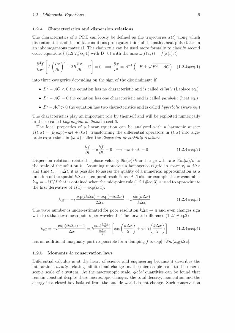
1.2.4 Characteristics and dispersion relations
The characteristics of a PDE can loosly be defined as the trajectories x(t) along whichdiscontinuities and the initial conditions propagate: think of the path a heat pulse takes inan inhomogeneous material. The chain rule can be used more formally to classify secondorder equations ( (1.2.2#eq.1) with D=0) with the ansatz f(x, t) = f(x(t), t)
∂2f
∂x2
[A
(∂x
∂t
)2
+ 2B∂x
∂t+ C
]= 0 =⇒ ∂x
∂t= A−1
(−B ±
√B2 −AC
)(1.2.4#eq.1)
into three categories depending on the sign of the discriminant: if
• B2 −AC < 0 the equation has no characteristic and is called elliptic (Laplace eq.)
• B2 −AC = 0 the equation has one characteristic and is called parabolic (heat eq.)
• B2−AC > 0 the equation has two characteristics and is called hyperbolic (wave eq.)
The characteristics play an important role by themself and will be exploited numericallyin the so-called Lagrangian methods in sect.6.
The local properties of a linear equation can be analyzed with a harmonic ansatzf(t, x) = f0 exp(−iωt + ikx), transforming the differential operators in (t, x) into alge-braic expressions in (ω, k) called the dispersion or stability relation:
∂f
∂t+ u
∂f
∂t= 0 =⇒ −ω + uk = 0 (1.2.4#eq.2)
Dispersion relations relate the phase velocity <e(ω)/k or the growth rate =m(ω)/k tothe scale of the solution k. Assuming moreover a homogeneous grid in space xj = j∆xand time tn = n∆t, it is possible to assess the quality of a numerical approximation as afunction of the spatial k∆x or temporal resolutions ωt. Take for example the wavenumberkeff = −if ′/f that is obtained when the mid-point rule (1.2.1#eq.3) is used to approximatethe first derivative of f(x) = exp(ikx):
keff = −iexp(ik∆x)− exp(−ik∆x)2∆x
= ksin(k∆x)k∆x
(1.2.4#eq.3)
The wave number is under-estimated for poor resolution k∆x→ π and even changes signwith less than two mesh points per wavelenth. The forward difference (1.2.1#eq.2)
keff = −iexp(ik∆x)− 1∆x
= ksin(k∆x
2 )k∆x
2
[cos(k∆x
2
)+ i sin
(k∆x
2
)](1.2.4#eq.4)
has an additional imaginary part responsible for a damping f ∝ exp[−=m(keff)∆x].
1.2.5 Moments & conservation laws
Differential calculus is at the heart of science and engineering because it describes theinteractions locally, relating infinitesimal changes at the microscopic scale to the macro-scopic scale of a system. At the macroscopic scale, global quantities can be found thatremain constant despite these microscopic changes: the total density, momentum and theenergy in a closed box isolated from the outside world do not change. Such conservation
10 1 INTRODUCTION
laws can in general be constructed by taking moments in phase space x, where the momentof order K a function f(x) is defined by
MK =∫
ΩdV xKf (1.2.5#eq.1)
Usually,M0 is the total density,M1 the total momentum andM2 the total energy in thesystem. Conservation laws provide useful self-consistency checks when PDEs are solvedin an approximate manner with the computer: deviations from the initial value can beused to monitor the quality of a numerical solution as it evolves in time.
1.3 Prototype problems
Here are some of the most important initial value problems /equations, illustrated in a1D periodic slab x ∈ [0;L[.
1.3.1 Advection
Also called convection, advection models the streaming of infinitesimal element in a fluid.It generally appears when a transport process is modeled in a Eulerian representationthrough the convective derivative
d
dtf ≡ ∂f
∂t+ u
∂f
∂x= 0 (1.3.1#eq.1)
For a constant advection velocity u, this can be solved analytically as f(x, t) = f0(x−ut)∀f0 ∈ C(Ω), showing explicitly the characteristic x = ut. Use the applet 7 to compute theevolution of a Gaussian pulse with an advection computed using the Lagrangian CIP/FEMmethod from sect.6. For a constant advection speed, the wave equation can be writtenin flux-conservative form
∂2h
∂t2− u2∂
2h
∂x2= 0 ⇐⇒ ∂
∂t
(fg
)− ∂
∂x
[(0 uu 0
)·(fg
)]= 0 (1.3.1#eq.2)
suggesting how the advection schemes may be generalized for wave problems.
1.3.2 Diffusion
At the microscopic scale, diffusion is related to a random walk and leads to the prototypeequation (exercise 1.4)
∂f
∂t−D∂
2f
∂x2= 0 (1.3.2#eq.1)
where D ≥ 0 is the so-called diffusion coefficient. For a homogeneous medium, the com-bined advection-diffusion equation
∂f
∂t+ u
∂f
∂x−D∂
2f
∂x2= 0 (1.3.2#eq.2)
7in the electronic version of the lecture notes http://pde.fusion.kth.se
1.3 Prototype problems 11
can be solved analytically in terms of a Green’s function (exercise 1.3)
f(x, t) =∫ +∞
−∞f0(x0)G(x− x0 − ut, t)dx0
G(x− x0 − ut, t) =1√π4Dt
exp(−(x− x0 − ut)2
4Dt
)(1.3.2#eq.3)
A numerical solution is generally required to solve the equation in an inhomogeneousmedium, where u(x), D(x):
∂f
∂t+ u
∂f
∂x− ∂
∂x
(D∂f
∂x
)= 0
Check the document on-line for an example of a numerical solution describing the advection-diffusion of a box computed with the finite element method from sect.3.
A harmonic ansatz in space and time f ∼ exp i(kx− ωt) yields the dispersion relation
ω = −iDk2 (1.3.2#eq.4)
and shows that short wavelengths (large k) are more strongly damped than long wave-lengths. Change the initial conditions to Cosine and model this numerically in the appletby altering the wavelength.
1.3.3 Dispersion
Dispersion occurs when different wavelengths propagate with different phase velocities.Take for example the third order dispersion equation
∂f
∂t− ∂3f
∂x3= 0 (1.3.3#eq.1)
A harmonic ansatz f ∼ exp i(kx− ωt) yields the phase velocity
−if(ω − k3) = 0 =⇒ ω
k= k2 (1.3.3#eq.2)
showing that short wavelengths (large k) propagate faster than long wavelengths (smallk). In the Korteweg-DeVries equation below, this explains why large amplitude solitonswith shorter wavelengths propagate more rapidly than low amplitudes solitons.
1.3.4 Wave-breaking
Wave-breaking is a non-linearity that can be particularly nicely understood when surfingat the see shore... where the shallow water steepens the waves until they break. It canalso be understood theoretically from the advection equation with a velocity proportionalto the amplitude u = f :
∂f
∂t+ f
∂f
∂x= 0 (1.3.4#eq.1)
As a local maximum (large f) propagates faster than a local minimum (small f) both willeventually meet and and the function becomes multi-valued, causing the wave (and our
12 1 INTRODUCTION
numerical schemes) to break. Sometimes, this wave-breaking is balanced by a competingmechanism. This is the case in the Burger equation for shock-waves
∂f
∂t+ f
∂f
∂x−D∂
2f
∂x2= 0 (1.3.4#eq.2)
where the creation of a shock front (with short wavelengths) is physically limited by adiffusion — damping the short wavelengths (1.3.2#eq.4). Check the document on-lineto see a shock formation computed using a 2-levels explicit finite difference scheme fromsect.2.
Another example, where the wave-breaking is balanced by dispersion leads to theKorteweg-DeVries equation for solitons
∂f
∂t+ f
∂f
∂x+ b
∂3f
∂x3= 0 (1.3.4#eq.3)
The on-line document shows how large amplitudes solitons (short wavelengths) propagatefaster than lower amplitudes (long wavelength).
1.3.5 Schrodinger
Choosing units where Planck’s constant ~ = 1 and the mass m = 1/2, its appears clearlythat the time-dependent Schrodinger equation is special type of wave / diffusion equation:
i∂ψ
∂t= Hψ with H(x) = − ∂2
∂x2+ V (x) (1.3.5#eq.1)
In quantum mechanics, such a Schrodinger equation evolves the complex wave-function|ψ >= ψ(x, t) that describes the probability < ψ|ψ >=
∫Ω |ψ|2dx of finding a particle in a
given interval Ω = [xL;xR]. Take the simplest example of a free particle modeled with awave-packet in a periodic domain with a constant potential V (x) = 0. The JBONE appleton-line shows the evolution of a low enery E = − < ψ|∂2
x|ψ > (long wavelength) particleinitially known with a rather good accuracy in space (narrow Gaussian envelope): thewave-function <e(ψ) (blue line) oscillates and the probability density |ψ|2 quickly spreadsout (black line) — reproducing Heisenberg’s famous uncertainty principle.
1.4 Discretization
Differential equations are solved numerically by evolving a discrete set of values fj,j = 1, N and by taking small steps in time ∆t to approximate what really should be acontinuous function of space and time f(x, t), x ∈ [a; b], t ≥ t0. Unfortunately, there is nouniversal method. Rather than adopting the favorite of a “local guru”, your choice for adiscretization should really depend on
• the structure of the solution (continuity, regularity, precision), the post-processing(filters) and the diagnostics (Fourier spectrum) that are expensive but might beanyway required
• the boundary conditions, which can be difficult to implement depending on themethod
• the structure of the differential operator (the formulation, the computational costin memory×time, the numerical stability) and the computer architecture (vectoriza-tion, parallelization).
1.4 Discretization 13
This course is a lot about advantages and limitations of different methods; it aims atgiving you a broad knowledge, so that you to make the optimal choices and that allowsyou to pursue with relatively advanced literature when this becomes necessary.
1.4.1 Convergence
The most important aspect of a numerical approximation of a continuous function with afinite number of discrete values is that this approximation converges to the exact value asmore information is gathered (exercise 1.5). This convergence can be defined locally forany arbitrary point in space / time (more restrictive) or by monitoring a global quantity(more permissive).
Take for example the function f(x) = xα in [0; 1] discretized using a homogeneous meshwith N values measured in the middle of each interval at xn = (n+ 1/2)/N . The lowestorder approximation f(0) ≈ f (N)(x0) = (2N)−α converges at the origin provided α ≥ 0.The convergence rate can be estimated from a geometric sequence of approximations f (i),obtained by successively doubling the numerical resolution i = N, 2N, 4N
r =ln[(f (N) − f (2N))/(f (2N) − f (4N))
]ln[2]
(1.4.1#eq.1)
For the example above, this gives a local convergence rate r = α when α > 0. Using themid-point rule (sect.3.3)
∫ 10 f(x)dx ≈
∑Nn=0 x
αn∆x with ∆x = 1/N , global convergence is
achieved when α > −1; because of the weak singularity, the rate however drops from theO[(∆x)2] expected for “smooth” functions to r ' 1.5, 0.5, 0.2 when α = 0.5,−0.5,−0.8.
1.4.2 Sampling on a grid
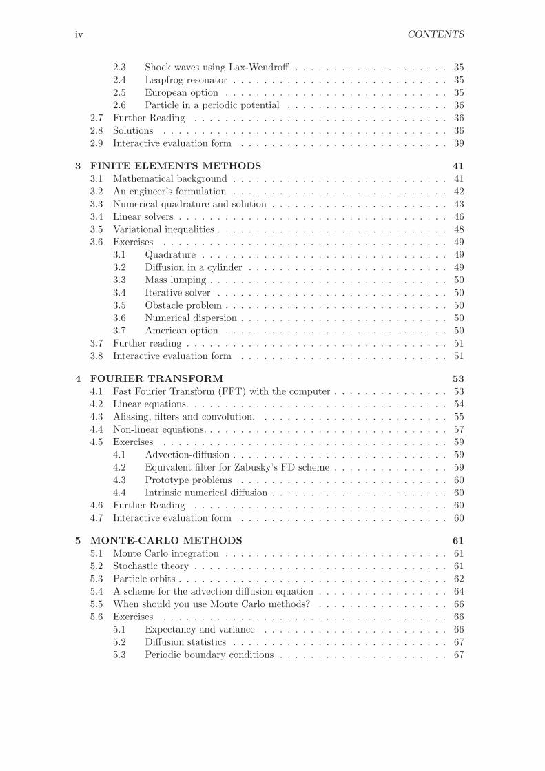
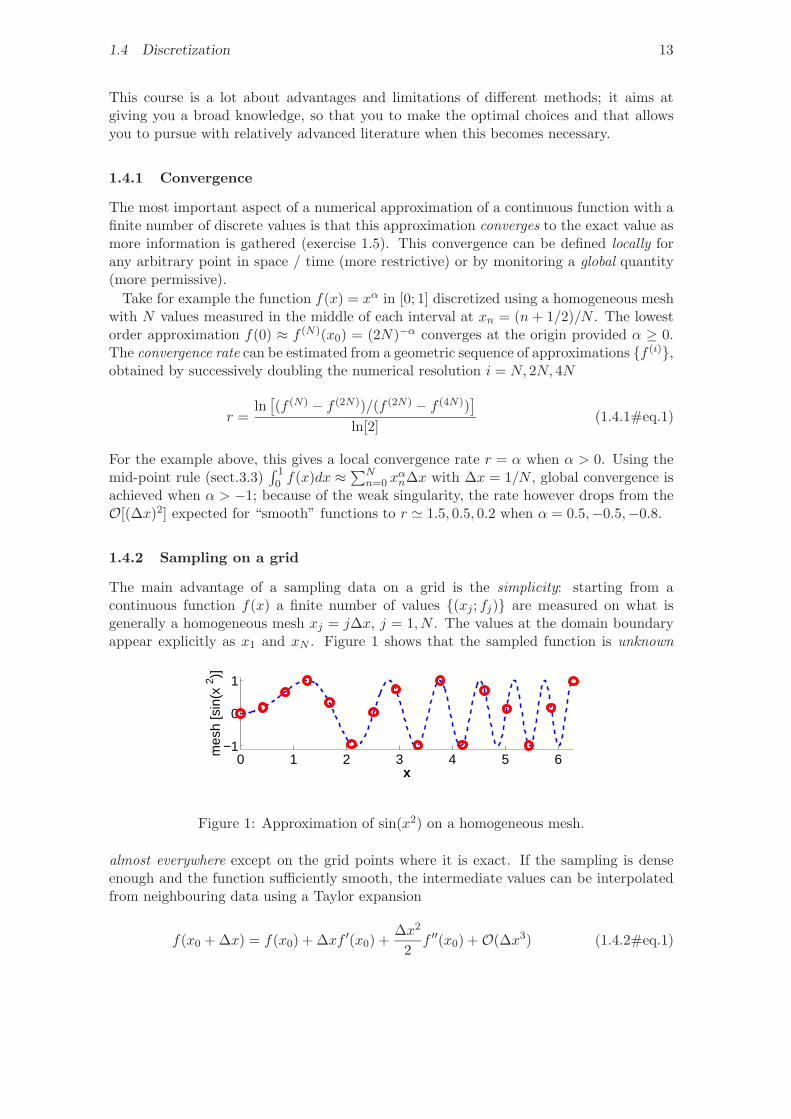
The main advantage of a sampling data on a grid is the simplicity: starting from acontinuous function f(x) a finite number of values (xj; fj) are measured on what isgenerally a homogeneous mesh xj = j∆x, j = 1, N . The values at the domain boundaryappear explicitly as x1 and xN . Figure 1 shows that the sampled function is unknown
0 1 2 3 4 5 6−1
0
1
mes
h [s
in(x
2 )]
x
Figure 1: Approximation of sin(x2) on a homogeneous mesh.
almost everywhere except on the grid points where it is exact. If the sampling is denseenough and the function sufficiently smooth, the intermediate values can be interpolatedfrom neighbouring data using a Taylor expansion
f(x0 + ∆x) = f(x0) + ∆xf ′(x0) +∆x2
2f ′′(x0) +O(∆x3) (1.4.2#eq.1)
14 1 INTRODUCTION
Derivatives are obtained by finite differencing from neighboring locations
fj+1 ≡ f(xj + ∆x) = fj + ∆xf ′j +∆x2
2f ′′j + . . .
fj−1 ≡ f(xj −∆x) = fj −∆xf ′j +∆x2
2f ′′j + . . .
leading to the formulas for the k-th derivative f (k) from Abramowitz [2] §25.1.2
f(2n)j =
2n∑k=0
(−1)k(
2nk
)fj+n−k (1.4.2#eq.2)
f(2n+1)j+1/2 =
2n+1∑k=0
(−1)k(
2n+ 1k
)fj+n+1−k (1.4.2#eq.3)(
nk
)=
n(n− 1) · · · (n− k + 1)k!
Note that a discretization on a grid is non-compact: the convergence depends not onlyon the initial discretisation, but also on the interpolation used a posteriori to reconstructthe data between the mesh points.
1.4.3 Finite elements
Following the spirit of Hilbert space methods, a function f(x) is decomposed on a completeset of nearly orthogonal basis functions ej ∈ B
f(x) =N∑j=1
fjej(x) (1.4.3#eq.1)
These finite-elements (FEM) basis functions span only as far as the neighboring meshpoints; most common are the normalized “roof-tops”
ej(x) =
(x− xj−1)/(xj − xj−1) x ∈ [xj−1;xj](xj+1 − x)/(xj+1 − xj) x ∈ [xj;xj+1]
(1.4.3#eq.2)
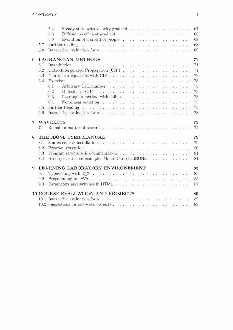
which yield a piecewise linear approximation for f(x) and a piecewise constant derivativef ′(x) defined almost everywhere in the interval [x1;xN ].
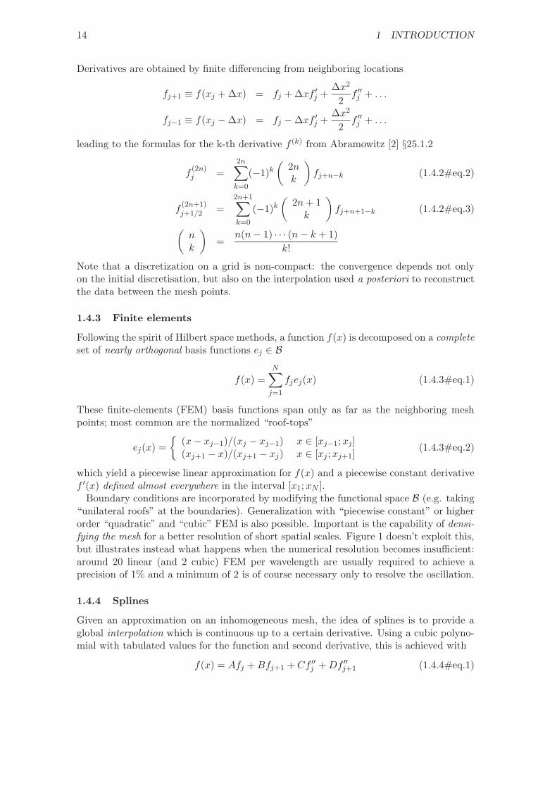
Boundary conditions are incorporated by modifying the functional space B (e.g. taking“unilateral roofs” at the boundaries). Generalization with “piecewise constant” or higherorder “quadratic” and “cubic” FEM is also possible. Important is the capability of densi-fying the mesh for a better resolution of short spatial scales. Figure 1 doesn’t exploit this,but illustrates instead what happens when the numerical resolution becomes insufficient:around 20 linear (and 2 cubic) FEM per wavelength are usually required to achieve aprecision of 1% and a minimum of 2 is of course necessary only to resolve the oscillation.
1.4.4 Splines
Given an approximation on an inhomogeneous mesh, the idea of splines is to provide aglobal interpolation which is continuous up to a certain derivative. Using a cubic polyno-mial with tabulated values for the function and second derivative, this is achieved with
f(x) = Afj +Bfj+1 + Cf ′′j +Df ′′j+1 (1.4.4#eq.1)
1.4 Discretization 15
0 1 2 3 4 5 6−1
0
1
LFE
M [s
in(
x 2 )]
0 1 2 3 4 5 60
1
2 e
5 −> f
5 =−0.947
x
Figure 1: Approximation of sin(x2) with roof-top linear finite elements.
A(x) = (xj+1 − x)/(xj+1 − xj) B(x) = 1−AC(x) = (xj+1 − xj)2(A3 −A)/6 D(x) = (xj+1 − xj)2(B3 −B)/6
from which it is straight forward to derive
f ′(x) =fj+1 − fjxj+1 − xj
− 3A2 − 16
(xj+1 − xj)f ′′j +3B2 − 1
6(xj+1 − xj)f ′′j+1 (1.4.4#eq.2)
f ′′(x) = Af ′′j +Bf ′′j+1 (1.4.4#eq.3)
Usually f ′′i , i = 1, N is calculated rather than measured: requiring that f ′(x) is continuousfrom one interval to another (1.4.4#eq.2) leads to a tridiagonal system for j = 2, N − 1
xj − xj−1
6f ′′j−1 +
xj+1 − xj−1
3f ′′j +
xj+1 − xj6
f ′′j+1 =fj+1 − fjxj+1 − xj
− fj − fj−1
xj − xj−1
(1.4.4#eq.4)
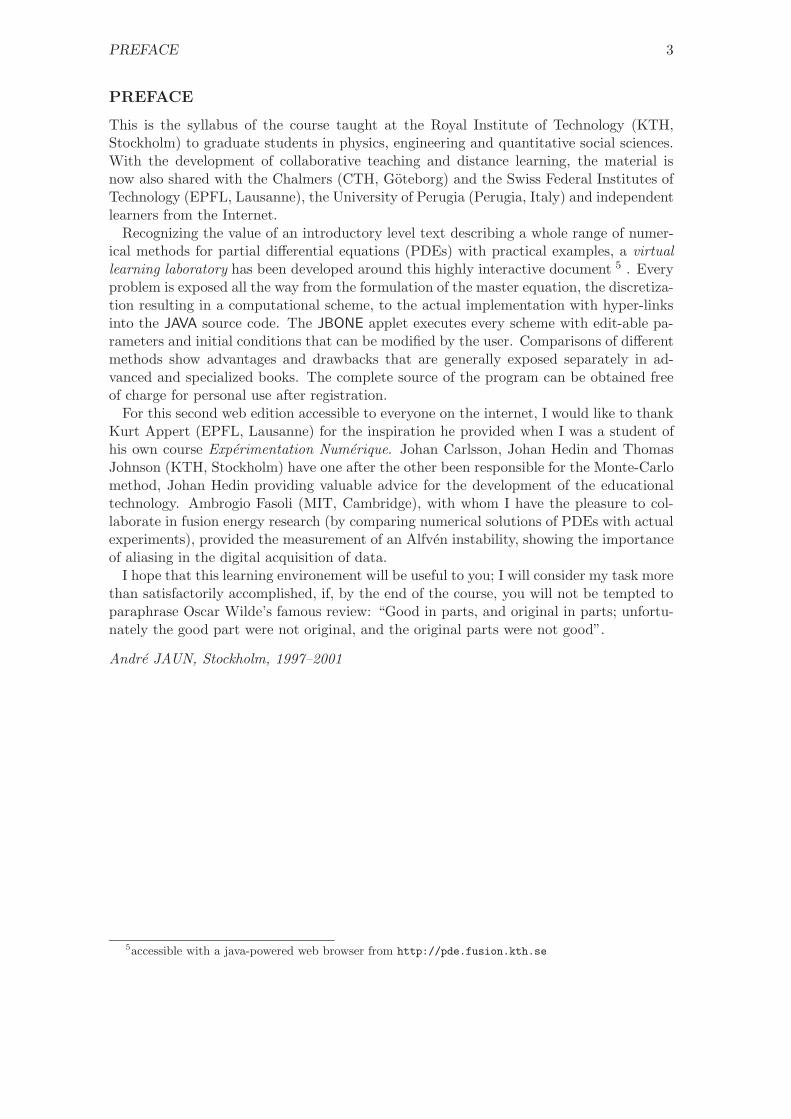
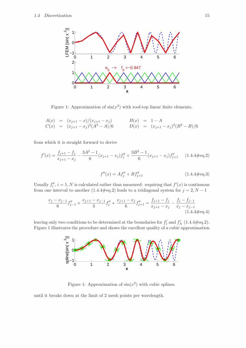
leaving only two conditions to be determined at the boundaries for f ′1 and f ′N (1.4.4#eq.2).Figure 1 illustrates the procedure and shows the excellent quality of a cubic approximation
0 1 2 3 4 5 6−1
0
1
splin
e[si
n( x
2 )]
x
Figure 1: Approximation of sin(x2) with cubic splines.
until it breaks down at the limit of 2 mesh points per wavelength.
16 1 INTRODUCTION
1.4.5 Harmonic functions
A harmonic decomposition is obtained from discrete Fourier transform (DFT) assuminga regular mesh and a periodicity L. Using the notations xm = m∆x = mL/M andkm = 2πm/L, the forward and backward transformations are given by:
f(km) =1M
M−1∑j=0
f(xj)W−kmxj , W = exp(2πi/M) (1.4.5#eq.1)
f(xj) =M−1∑m=0
f(km)W+kmxj (1.4.5#eq.2)
If M is a power of 2, the number of operation can be dramatically reduced from 8M2 toM log2M with the fast Fourier transform (FFT), applying recursively the decomposition
f(km) =1M
2M−1∑j=0
f(xj)W−kmxj =∑j even
+∑j odd
=
=1M
2M−1−1∑j=0
f(x2j)(W 2)−kmxj +W−km
M
2M−1−1∑j=0
f(x2j+1)(W 2)−kmxj
(1.4.5#eq.3)
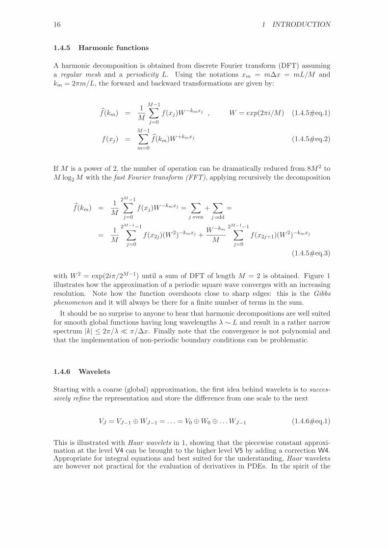
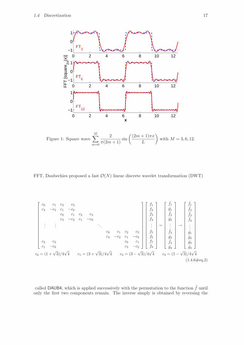
with W 2 = exp(2iπ/2M−1) until a sum of DFT of length M = 2 is obtained. Figure 1illustrates how the approximation of a periodic square wave converges with an increasingresolution. Note how the function overshoots close to sharp edges: this is the Gibbsphenomenon and it will always be there for a finite number of terms in the sum.
It should be no surprise to anyone to hear that harmonic decompositions are well suitedfor smooth global functions having long wavelengths λ ∼ L and result in a rather narrowspectrum |k| ≤ 2π/λ π/∆x. Finally note that the convergence is not polynomial andthat the implementation of non-periodic boundary conditions can be problematic.
1.4.6 Wavelets
Starting with a coarse (global) approximation, the first idea behind wavelets is to succes-sively refine the representation and store the difference from one scale to the next
VJ = VJ−1 ⊕WJ−1 = . . . = V0 ⊕W0 ⊕ . . .WJ−1 (1.4.6#eq.1)
This is illustrated with Haar wavelets in 1, showing that the piecewise constant approxi-mation at the level V4 can be brought to the higher level V5 by adding a correction W4.Appropriate for integral equations and best suited for the understanding, Haar waveletsare however not practical for the evaluation of derivatives in PDEs. In the spirit of the
1.4 Discretization 17
0 2 4 6 8 10 12−1
0
1
FT3
0 2 4 6 8 10 12−1
0
1F
FT
[squ
are 2π
(x)]
FT6
0 2 4 6 8 10 12−1
0
1
FT12
x
Figure 1: Square waveM∑m=0
2π(2m+ 1)
sin(
(2m+ 1)πxL
)with M = 3, 6, 12.
FFT, Daubechies proposed a fast O(N) linear discrete wavelet transformation (DWT)
c0 c1 c2 c3c3 −c2 c1 −c0
c0 c1 c2 c3c3 −c2 c1 −c0
......
. . .c0 c1 c2 c3c3 −c2 c1 −c0
c2 c3 c0 c1c1 −c0 c3 −c2
f1
f2
f3
f4
...f5
f6
f7
f8
=
f1
g1
f2
g2
...f3
g3
f4
g4
→
f1
f2
f3
f4
...g1
g2
g3
g4
c0 = (1 +
√3)/4√
4 c1 = (3 +√
3)/4√
4 c2 = (3−√
3)/4√
4 c3 = (1−√
3)/4√
4(1.4.6#eq.2)
called DAUB4, which is applied successively with the permutation to the function f untilonly the first two components remain. The inverse simply is obtained by reversing the
18 1 INTRODUCTION
0 1 2 3 4 5 6−1
0
1 V5
0 1 2 3 4 5 6−1
0
1 V4H
aar
wav
elet
s [s
in(
x 2 )]
0 1 2 3 4 5 6−1
0
1 W4
x
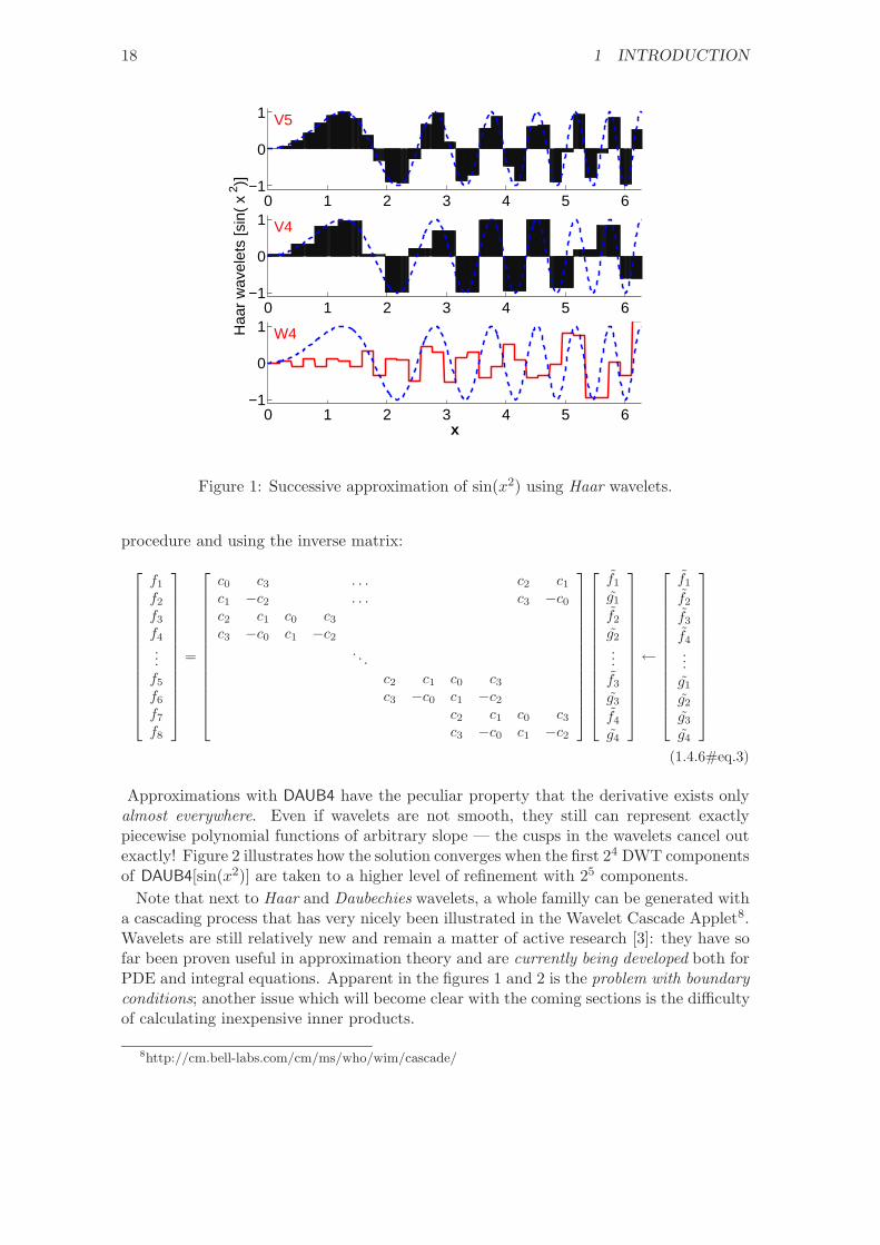
Figure 1: Successive approximation of sin(x2) using Haar wavelets.
procedure and using the inverse matrix:
f1
f2
f3
f4
...f5
f6
f7
f8
=
c0 c3 . . . c2 c1c1 −c2 . . . c3 −c0c2 c1 c0 c3c3 −c0 c1 −c2
. . .c2 c1 c0 c3c3 −c0 c1 −c2
c2 c1 c0 c3c3 −c0 c1 −c2
f1
g1
f2
g2
...f3
g3
f4
g4
←
f1
f2
f3
f4
...g1
g2
g3
g4
(1.4.6#eq.3)
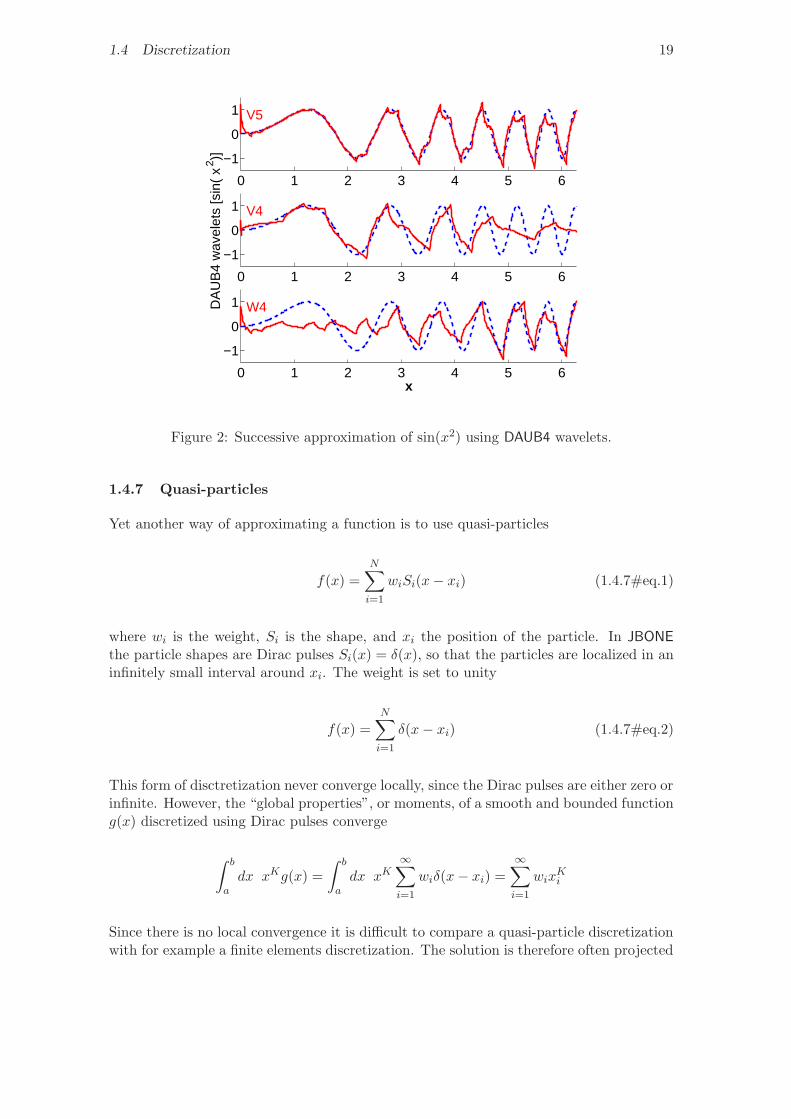
Approximations with DAUB4 have the peculiar property that the derivative exists onlyalmost everywhere. Even if wavelets are not smooth, they still can represent exactlypiecewise polynomial functions of arbitrary slope — the cusps in the wavelets cancel outexactly! Figure 2 illustrates how the solution converges when the first 24 DWT componentsof DAUB4[sin(x2)] are taken to a higher level of refinement with 25 components.
Note that next to Haar and Daubechies wavelets, a whole familly can be generated witha cascading process that has very nicely been illustrated in the Wavelet Cascade Applet8.Wavelets are still relatively new and remain a matter of active research [3]: they have sofar been proven useful in approximation theory and are currently being developed both forPDE and integral equations. Apparent in the figures 1 and 2 is the problem with boundaryconditions; another issue which will become clear with the coming sections is the difficultyof calculating inexpensive inner products.
8http://cm.bell-labs.com/cm/ms/who/wim/cascade/
1.4 Discretization 19
0 1 2 3 4 5 6
−1
0
1 V5
0 1 2 3 4 5 6
−1
0
1 V4D
AU
B4
wav
elet
s [s
in(
x 2 )]
0 1 2 3 4 5 6
−1
0
1 W4
x
Figure 2: Successive approximation of sin(x2) using DAUB4 wavelets.
1.4.7 Quasi-particles
Yet another way of approximating a function is to use quasi-particles
f(x) =N∑i=1
wiSi(x− xi) (1.4.7#eq.1)
where wi is the weight, Si is the shape, and xi the position of the particle. In JBONEthe particle shapes are Dirac pulses Si(x) = δ(x), so that the particles are localized in aninfinitely small interval around xi. The weight is set to unity
f(x) =N∑i=1
δ(x− xi) (1.4.7#eq.2)
This form of disctretization never converge locally, since the Dirac pulses are either zero orinfinite. However, the “global properties”, or moments, of a smooth and bounded functiong(x) discretized using Dirac pulses converge
∫ b
adx xKg(x) =
∫ b
adx xK
∞∑i=1
wiδ(x− xi) =∞∑i=1
wixKi
Since there is no local convergence it is difficult to compare a quasi-particle discretizationwith for example a finite elements discretization. The solution is therefore often projected
20 1 INTRODUCTION
onto a set of basis functions ϕjNϕj=1
fϕ(x) =Nϕ∑j=1
∫f(x)ϕj(x)) dξ√∫
ϕj(ξ)2 dξϕj(x)
=Nϕ∑j=1
N∑i=1
∫wiδ(ξ − xi)ϕj(ξ) dξ√∫
ϕj(ξ)2 dξϕj(x)
=Nϕ∑j=1
N∑i=1
wiϕj(xi)√∫ϕj(ξ)2 dξ
ϕj(x)
(1.4.7#eq.3)
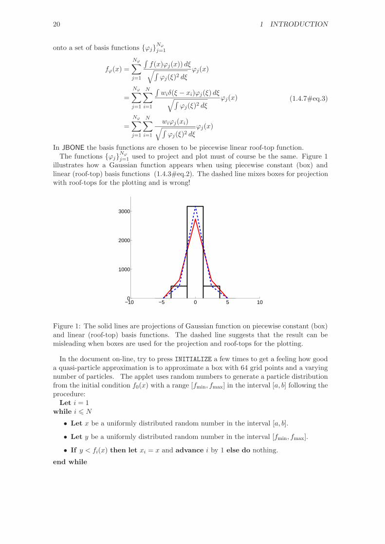
In JBONE the basis functions are chosen to be piecewise linear roof-top function.The functions ϕjNϕj=1 used to project and plot must of course be the same. Figure 1
illustrates how a Gaussian function appears when using piecewise constant (box) andlinear (roof-top) basis functions (1.4.3#eq.2). The dashed line mixes boxes for projectionwith roof-tops for the plotting and is wrong!
−10 −5 0 5 100
1000
2000
3000
Figure 1: The solid lines are projections of Gaussian function on piecewise constant (box)and linear (roof-top) basis functions. The dashed line suggests that the result can bemisleading when boxes are used for the projection and roof-tops for the plotting.
In the document on-line, try to press INITIALIZE a few times to get a feeling how gooda quasi-particle approximation is to approximate a box with 64 grid points and a varyingnumber of particles. The applet uses random numbers to generate a particle distributionfrom the initial condition f0(x) with a range [fmin, fmax] in the interval [a, b] following theprocedure:
Let i = 1while i 6 N• Let x be a uniformly distributed random number in the interval [a, b].
• Let y be a uniformly distributed random number in the interval [fmin, fmax].
• If y < fi(x) then let xi = x and advance i by 1 else do nothing.
end while
1.5 Exercises 21
1.5 Exercises
1.0 E-publishing
Familiarize yourself with the electronic submission of assignments and use the discussionforums. Follow the TEXlink to type a small text with formulas; learn how to interpretthe error messages. Change the default applet parameters to compute the diffusion ofa harmonic function and determine the largest diffusion coefficient that seems to give areasonable result (this will be discussed in the next chapter). Read the rules governingthe discussion forums and introduce yourself, telling a few words about your backgroundand interests; chat with your colleagues...
1.1 Stiff ODE
Assuming boundary conditions u(0) = 1; v(0) = 0, use the MATLAB commands ode23and ode23s to integrate
u′ = 998u+ 1998vv′ = −999u− 1999v
in the interval [0; 1]. Use the variable transformation u = 2y − z; v = −y + z to comparewith an analytical solution and show that the problem is stiff.
1.2 Predator-Prey model
Study the solutions of the famous Volterra Predator-Prey model
dy1
dt= αy1 − βy1y2;
dy2
dt= −γy2 + δy1y2
that predicts the evolution of two populations (y1 the number of preys and y2 the numberof predators) depending on each other for their existence. Assume α = β = γ = δ = 1and use MATLAB to study periodic solutions in the interval [0; 4]× [0; 4]. Is there a wayto reach a natural equilibrium?
1.3 Fourier-Laplace transform
Solve the advection-diffusion analytically in an infinite 1D slab assuming both the ad-vection speed u and the diffusion coefficient D constant. Hint: use a Fourier-Laplacetransform to first determine the evolution of the Green’s function G(x − x0, t) startingfrom an initial condition δ(x − x0). Superpose to describe an arbitrary initial functionf0(x).
1.4 Random-walk
Determine the diffusion constant for a random-walk process with steps of a typical durationτ and mean free path λ =
√〈v2〉τ . Hint: calculate first the RMS displacement
⟨z2⟩
(t)of the position after a large number M = t/τ of statistically independent steps took place.Take the second moment of the diffusion equation and integrate by parts to calculate theaverage z2(t). Conclude by relating each other using the ergodicity theorem.
22 1 INTRODUCTION
1.5 Convergence
Calculate a discrete representation of sin(kx), kx ∈ [0; 2π] for atleast four numericalapproximations introduced in the first chapter. Sketch (with words) the relative localerror for kx = 1 and show how the approximations converge to the analytical value whenthe numerical resolution increases. What about the first derivative?
1.6 Laplacian in 2D
Use a Taylor expansion to calculate an approximation of the Laplacian operator on arectangular grid ∆x = ∆y = h. Repeat the calculation for an evenly-spaced, equilateraltriangular mesh. Hint: determine the coordinate transformation for a rotation of 0, 60,120o and apply the chain rule for partial derivatives in all the three direction.
1.7 Hypercube
Show that when using a regular grid with n mesh points in each direction, most of thevalues sampled in hypercube of large dimension N land on the surface. Can you thinkof a discretization that is more appropriate? Hint: estimate the relative number of meshpoints within the volume with
(n−2n
)N , write it as an exponential and expand.
1.6 Further reading
• ODE, symplectic integration and stiff equations.Numerical Recipes [4] §16, 16.6, Sanz-Serna [5], Dahlquist [6] §13
• PDE properties.Fletcher [7] §2
• Interpolation and differentiation.Abramowitz [2] §25.2–25.3, Dahlquist [6] §4.6, 4.7, Fletcher [7] §3.2, 3.3
• FEM approximation.Fletcher [7] §5.3, Johnson [8], Appert [9]
• Splines.Numerical Recipes [4] §12.0–12.2, Dahlquist [6] §4.8
• FFT.Numerical Recipes [4] §12.0–12.2
• Wavelets.Numerical Recipes [4] §13.10, www.wavelet.org9 [3]
• Software.Guide to Available Mathematical Software10 [10], Computer Physics Communica-tions Library11 [11]
9http://www.wavelet.org/wavelet/index.html10http://gams.nist.gov11http://www.cpc.cs.qub.ac.uk/cpc/
1.7 Solutions 23
1.7 Solutions
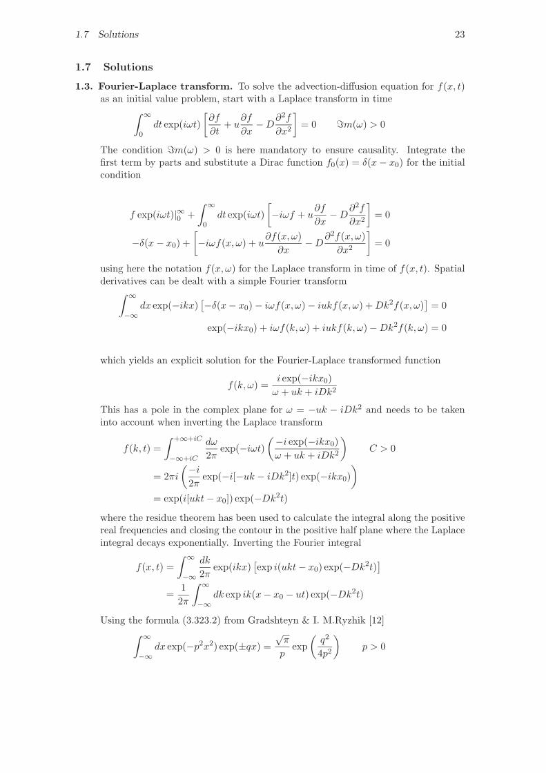
1.3. Fourier-Laplace transform. To solve the advection-diffusion equation for f(x, t)as an initial value problem, start with a Laplace transform in time∫ ∞
0dt exp(iωt)
[∂f
∂t+ u
∂f
∂x−D∂
2f
∂x2
]= 0 =m(ω) > 0
The condition =m(ω) > 0 is here mandatory to ensure causality. Integrate thefirst term by parts and substitute a Dirac function f0(x) = δ(x− x0) for the initialcondition
f exp(iωt)|∞0 +∫ ∞
0dt exp(iωt)
[−iωf + u
∂f
∂x−D∂
2f
∂x2
]= 0
−δ(x− x0) +[−iωf(x, ω) + u
∂f(x, ω)∂x
−D∂2f(x, ω)∂x2
]= 0
using here the notation f(x, ω) for the Laplace transform in time of f(x, t). Spatialderivatives can be dealt with a simple Fourier transform∫ ∞
−∞dx exp(−ikx)
[−δ(x− x0)− iωf(x, ω)− iukf(x, ω) +Dk2f(x, ω)
]= 0
exp(−ikx0) + iωf(k, ω) + iukf(k, ω)−Dk2f(k, ω) = 0
which yields an explicit solution for the Fourier-Laplace transformed function
f(k, ω) =i exp(−ikx0)ω + uk + iDk2
This has a pole in the complex plane for ω = −uk − iDk2 and needs to be takeninto account when inverting the Laplace transform
f(k, t) =∫ +∞+iC
−∞+iC
dω
2πexp(−iωt)
(−i exp(−ikx0)ω + uk + iDk2
)C > 0
= 2πi(−i2π
exp(−i[−uk − iDk2]t) exp(−ikx0))
= exp(i[ukt− x0]) exp(−Dk2t)
where the residue theorem has been used to calculate the integral along the positivereal frequencies and closing the contour in the positive half plane where the Laplaceintegral decays exponentially. Inverting the Fourier integral
f(x, t) =∫ ∞−∞
dk
2πexp(ikx)
[exp i(ukt− x0) exp(−Dk2t)
]=
12π
∫ ∞−∞
dk exp ik(x− x0 − ut) exp(−Dk2t)
Using the formula (3.323.2) from Gradshteyn & I. M.Ryzhik [12]∫ ∞−∞
dx exp(−p2x2) exp(±qx) =√π
pexp
(q2
4p2
)p > 0
24 1 INTRODUCTION
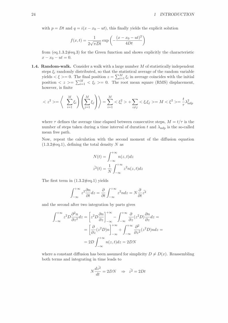
with p = Dt and q = i(x− x0 − ut), this finally yields the explicit solution
f(x, t) =1
2√πDt
exp(−(x− x0 − ut)2
4Dt
)from (eq.1.3.2#eq.3) for the Green function and shows explicitly the characteristicx− x0 − ut = 0.
1.4. Random-walk. Consider a walk with a large number M of statistically independentsteps ξi randomly distributed, so that the statistical average of the random variableyields < ξ >= 0. The final position z =
∑Mi=1 ξi in average coincides with the initial
position < z >=∑M
i=1 < ξi >= 0. The root mean square (RMS) displacement,however, is finite
< z2 >=
⟨(M∑i=1
ξi
) M∑j=1
ξj
⟩ =M∑i=1
< ξ2i > +
∑i6=j
< ξiξj >= M < ξ2 >=t
τλ2
mfp
where τ defines the average time elapsed between consecutive steps, M = t/τ is thenumber of steps taken during a time interval of duration t and λmfp is the so-calledmean free path.
Now, repeat the calculation with the second moment of the diffusion equation(1.3.2#eq.1), defining the total density N as
N(t) =∫ +∞
−∞n(z, t)dz
z2(t) =1N
∫ +∞
−∞z2n(z, t)dz
The first term in (1.3.2#eq.1) yields∫ +∞
−∞z2∂n
∂tdz =
∂
∂t
∫ +∞
−∞z2ndz = N
∂
∂tz2
and the second after two integration by parts gives∫ +∞
−∞z2D
∂2n
∂z2dz =
[z2D
∂n
∂z
]+∞
−∞−∫ +∞
−∞
∂
∂z(z2D)
∂n
∂zdz =
=[∂
∂z(z2D)n
]+∞
−∞+∫ +∞
−∞
∂2
∂z2(z2D)ndz =
= 2D∫ +∞
−∞n(z, t)dz = 2DN
where a constant diffusion has been assumed for simplicity D 6= D(x). Reassemblingboth terms and integrating in time leads to
Ndz2
dt= 2DN ⇒ z2 = 2Dt
1.8 Interactive evaluation form 25
The ergodicity theorem is finally used to identify the statistical average < X > withthe mean value of a continuous variable X, leading to the well known identity
D =λ2
mfp
2τ.
The theory of stochastic processes behind the Monte-Carlo Method is rather so-phisticated and will be introduced later in sect.5. From the calculation above, itis however possible to conclude now already that the evolution of a large numberof independent particles following a random walk can be described implemented inJBONE with the simple algorithm
for(int j = 0; j < numberOfParticles; j++)particlePosition[j] += random.nextGaussian() *Math.sqrt(2 * diffusCo * timeStep);
and describes in fact a diffusion.
1.8 Interactive evaluation form
Your anonymous opinion is precious. Please fill-in our anonymous form in the web edition.Thank you very much in advance for your collaboration!

26 1 INTRODUCTION
27
2 FINITE DIFFERENCES
2.1 Explicit 2 levels
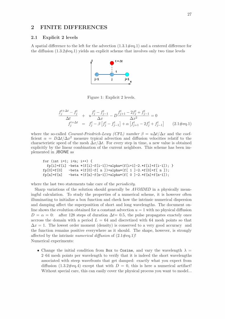
A spatial difference to the left for the advection (1.3.1#eq.1) and a centered difference forthe diffusion (1.3.2#eq.1) yields an explicit scheme that involves only two time levels
∆t + t
t
x
t
j−1 j j+1
Figure 1: Explicit 2 levels.
f t+∆tj − f tj
∆t+ u
f tj − f tj−1
∆x−D
f tj+1 − 2f tj + f tj−1
∆x2= 0
f t+∆tj = f tj − β
[f tj − f tj−1
]+ α
[f tj+1 − 2f tj + f tj−1
](2.1#eq.1)
where the so-called Courant-Friedrich-Lewy (CFL) number β = u∆t/∆x and the coef-ficient α = D∆t/∆x2 measure typical advection and diffusion velocities relatif to thecharacteristic speed of the mesh ∆x/∆t. For every step in time, a new value is obtainedexplicitly by the linear combination of the current neighbors. This scheme has been im-plemented in JBONE as
for (int i=1; i<n; i++) fp[i]=f[i] -beta *(f[i]-f[i-1])+alpha*(f[i+1]-2.*f[i]+f[i-1]);
fp[0]=f[0] -beta *(f[0]-f[ n ])+alpha*(f[ 1 ]-2.*f[0]+f[ n ]);fp[n]=f[n] -beta *(f[n]-f[n-1])+alpha*(f[ 0 ]-2.*f[n]+f[n-1]);
where the last two statements take care of the periodicity.Sharp variations of the solution should generally be AVOIDED in a physically mean-
ingful calculation. To study the properties of a numerical scheme, it is however oftenilluminating to initialize a box function and check how the intrinsic numerical dispersionand damping affect the superposition of short and long wavelengths. The document on-line shows the evolution obtained for a constant advection u = 1 with no physical diffusionD = α = 0: after 128 steps of duration ∆t= 0.5, the pulse propagates exactely onceaccross the domain with a period L = 64 and discretized with 64 mesh points so that∆x = 1. The lowest order moment (density) is conserved to a very good accuracy andthe function remains positive everywhere as it should. The shape, however, is stronglyaffected by the intrinsic numerical diffusion of (2.1#eq.1)!Numerical experiments:
• Change the initial condition from Box to Cosine, and vary the wavelength λ =2–64 mesh points per wavelength to verify that it is indeed the short wavelengthsassociated with steep wavefronts that get damped: exactly what you expect fromdiffusion (1.3.2#eq.4) except that with D = 0, this is here a numerical artifact!Without special care, this can easily cover the physical process you want to model...
28 2 FINITE DIFFERENCES
• Looking for a quick fix, you reduce the time step and the CFL number from β = 0.5down 0.1. What happens ? Adding further to the confusion, increase the time stepto exactly 1 and check what happens.
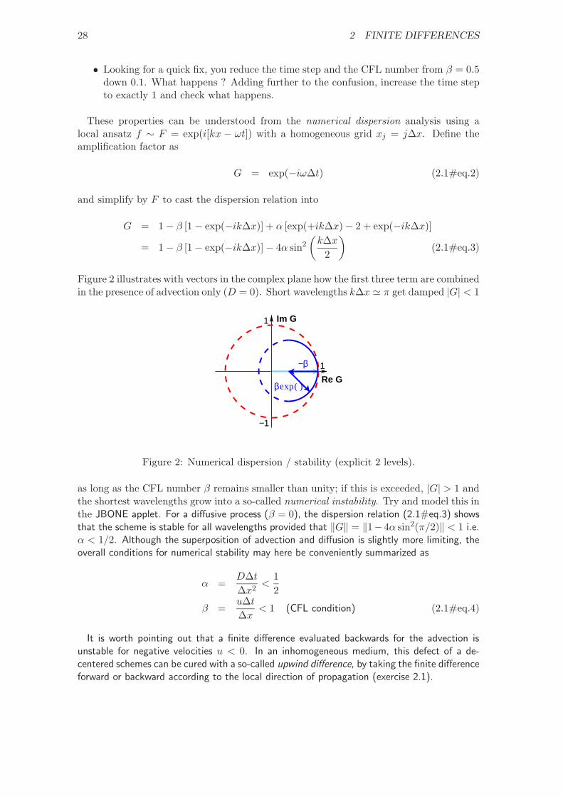
These properties can be understood from the numerical dispersion analysis using alocal ansatz f ∼ F = exp(i[kx − ωt]) with a homogeneous grid xj = j∆x. Define theamplification factor as
G = exp(−iω∆t) (2.1#eq.2)
and simplify by F to cast the dispersion relation into
G = 1− β [1− exp(−ik∆x)] + α [exp(+ik∆x)− 2 + exp(−ik∆x)]
= 1− β [1− exp(−ik∆x)]− 4α sin2
(k∆x
2
)(2.1#eq.3)
Figure 2 illustrates with vectors in the complex plane how the first three term are combinedin the presence of advection only (D = 0). Short wavelengths k∆x ' π get damped |G| < 1
−1
1 Im G
Re G
−β 1
βexp( )
Figure 2: Numerical dispersion / stability (explicit 2 levels).
as long as the CFL number β remains smaller than unity; if this is exceeded, |G| > 1 andthe shortest wavelengths grow into a so-called numerical instability. Try and model this inthe JBONE applet. For a diffusive process (β = 0), the dispersion relation (2.1#eq.3) showsthat the scheme is stable for all wavelengths provided that ‖G‖ = ‖1− 4α sin2(π/2)‖ < 1 i.e.α < 1/2. Although the superposition of advection and diffusion is slightly more limiting, theoverall conditions for numerical stability may here be conveniently summarized as
α =D∆t∆x2
<12
β =u∆t∆x
< 1 (CFL condition) (2.1#eq.4)
It is worth pointing out that a finite difference evaluated backwards for the advection isunstable for negative velocities u < 0. In an inhomogeneous medium, this defect of a de-centered schemes can be cured with a so-called upwind difference, by taking the finite differenceforward or backward according to the local direction of propagation (exercise 2.1).
2.2 Explicit 3 levels 29
∆t + t
t − t∆
x
t
j−1 j j+1
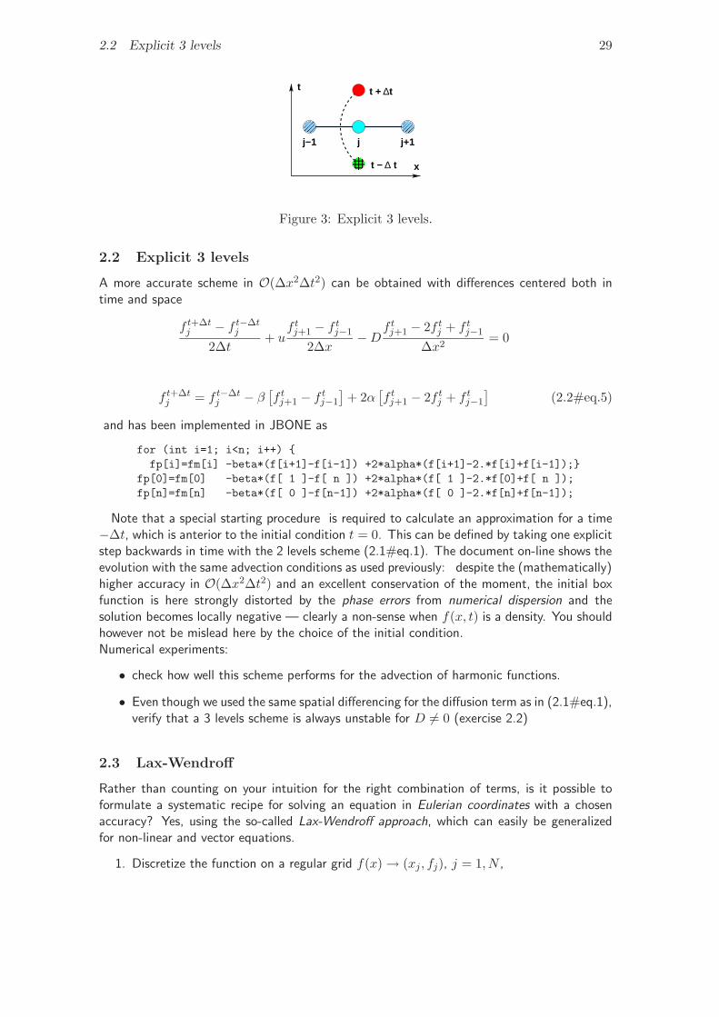
Figure 3: Explicit 3 levels.
2.2 Explicit 3 levels
A more accurate scheme in O(∆x2∆t2) can be obtained with differences centered both intime and space
f t+∆tj − f t−∆t
j
2∆t+ u
f tj+1 − f tj−1
2∆x−D
f tj+1 − 2f tj + f tj−1
∆x2= 0
f t+∆tj = f t−∆t
j − β[f tj+1 − f tj−1
]+ 2α
[f tj+1 − 2f tj + f tj−1
](2.2#eq.5)
and has been implemented in JBONE as
for (int i=1; i<n; i++) fp[i]=fm[i] -beta*(f[i+1]-f[i-1]) +2*alpha*(f[i+1]-2.*f[i]+f[i-1]);
fp[0]=fm[0] -beta*(f[ 1 ]-f[ n ]) +2*alpha*(f[ 1 ]-2.*f[0]+f[ n ]);fp[n]=fm[n] -beta*(f[ 0 ]-f[n-1]) +2*alpha*(f[ 0 ]-2.*f[n]+f[n-1]);
Note that a special starting procedure is required to calculate an approximation for a time−∆t, which is anterior to the initial condition t = 0. This can be defined by taking one explicitstep backwards in time with the 2 levels scheme (2.1#eq.1). The document on-line shows theevolution with the same advection conditions as used previously: despite the (mathematically)higher accuracy in O(∆x2∆t2) and an excellent conservation of the moment, the initial boxfunction is here strongly distorted by the phase errors from numerical dispersion and thesolution becomes locally negative — clearly a non-sense when f(x, t) is a density. You shouldhowever not be mislead here by the choice of the initial condition.Numerical experiments:
• check how well this scheme performs for the advection of harmonic functions.
• Even though we used the same spatial differencing for the diffusion term as in (2.1#eq.1),verify that a 3 levels scheme is always unstable for D 6= 0 (exercise 2.2)
2.3 Lax-Wendroff
Rather than counting on your intuition for the right combination of terms, is it possible toformulate a systematic recipe for solving an equation in Eulerian coordinates with a chosenaccuracy? Yes, using the so-called Lax-Wendroff approach, which can easily be generalizedfor non-linear and vector equations.
1. Discretize the function on a regular grid f(x)→ (xj , fj), j = 1, N ,
30 2 FINITE DIFFERENCES
2. Expand the differential operators in time using a Taylor series
f t+∆txj = f txj + ∆t
∂f
∂t
∣∣∣∣xj
+∆t2
2∂2f
∂t2
∣∣∣∣xj
+O(∆t3) (2.3#eq.6)
3. Substitute the time derivatives from the master equation. Using only advection (1.3.1#eq.1)here for illustration, this yields
f t+∆txj = f txj − u∆t
∂f
∂x
∣∣∣∣xj
+(u∆t)2
2∂2f
∂x2
∣∣∣∣xj
+O(∆t3) (2.3#eq.7)
4. Take centered differences for spatial operators
f t+∆tj = f tj −
β
2(f tj+1 − f tj−1
)+β2
2(f tj+1 − 2f tj + f tj−1
)+O(∆x3∆t3) (2.3#eq.8)
This procedure results in a second order advectionscheme which is explicit, centered and stableprovided that the CFL number β = u∆t/∆x remains below unity:
for (int i=1; i<n; i++) fp[i]=f[i] -0.5*beta *(f[i+1]-f[i-1])
+0.5*beta*beta*(f[i+1]-2.*f[i]+f[i-1]); fp[0]=f[0] -0.5*beta *(f[ 1 ]-f[ n ])
+0.5*beta*beta*(f[ 1 ]-2.*f[0]+f[ n ]);fp[n]=f[n] -0.5*beta *(f[ 0 ]-f[n-1])
+0.5*beta*beta*(f[ 0 ]-2.*f[n]+f[n-1]);
Numerical diffusion damps mainly the shorter wavelengths and distorts somewhat the boxfunction as it propagates.Numerical experiments:
• Test if this scheme works also for negative velocities.
• Explain what happens when you chose β = 1; why can you not rely on that?
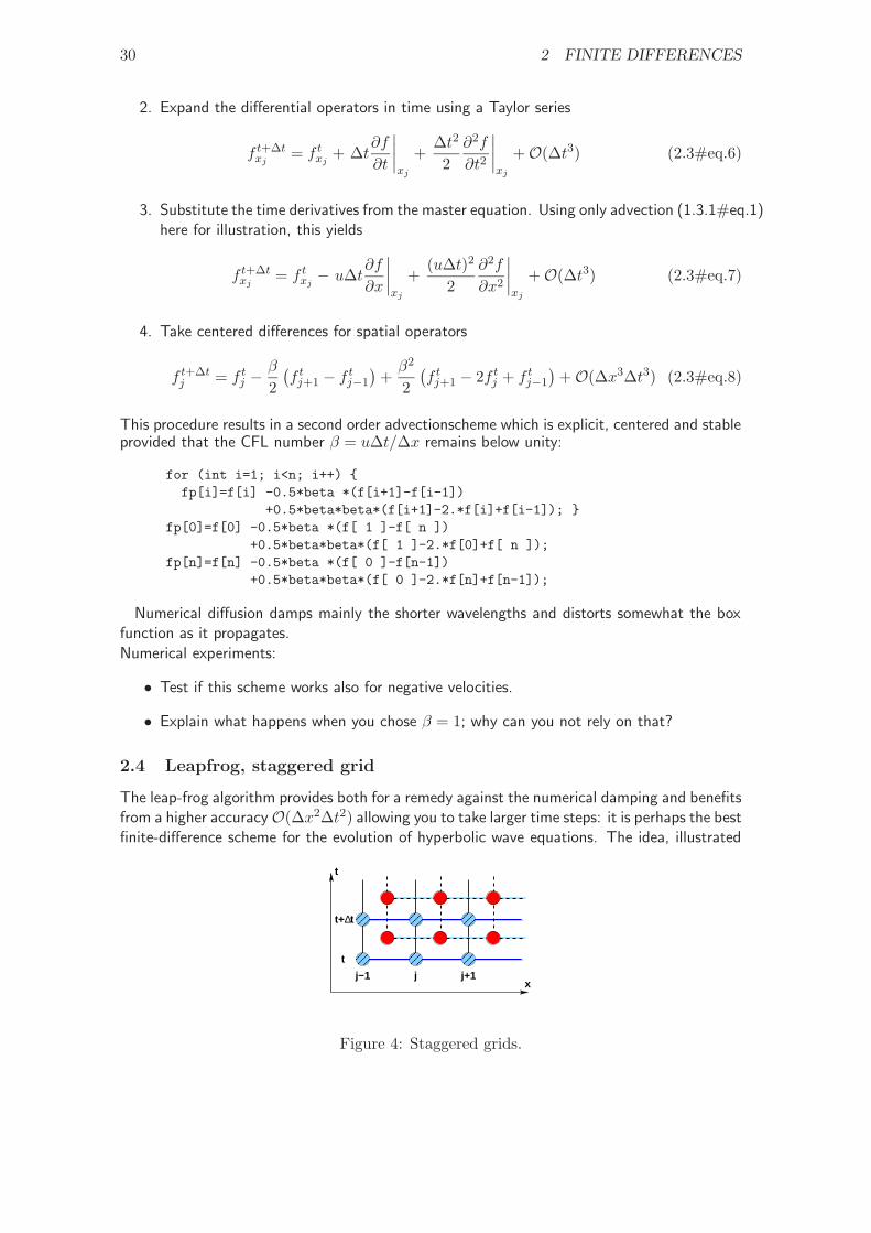
2.4 Leapfrog, staggered grid
The leap-frog algorithm provides both for a remedy against the numerical damping and benefitsfrom a higher accuracyO(∆x2∆t2) allowing you to take larger time steps: it is perhaps the bestfinite-difference scheme for the evolution of hyperbolic wave equations. The idea, illustrated
j+1j−1 j
t+ t∆
t
x
t
Figure 4: Staggered grids.
2.5 Implicit Crank-Nicholson 31
in figure 4, is to use so called staggered grids (where the mesh points are shifted with respectto each other by half an interval) and evaluate the solution using two functions of the form
1∆t
[f t+∆ti+1/2 − f
ti+1/2
]= u
∆x
[gt+∆t/2i+1 − gt+∆t/2
i
]1
∆t
[gt+∆t/2i − gt−∆t/2
i
]= u
∆x
[f ti+1/2 − f ti−1/2
] (2.4#eq.9)
This scheme suggests with scalar fields (f, g) how Maxwell’s equations can be convenientlysolved using the so-called finite differences in the time domain (FDTD) by using different grids
for the electric and the magnetic fields ( ~E, ~B) [2.7]. The leapfrog algorithm in JBONE hasbeen implemented as
for (int i=1; i<=n; i++) //time + time_stepfp[i]=f[i] -beta*(g[i]-g[i-1]);
fp[0]=f[0] -beta*(g[0]-g[n]);for (int i=0; i<=n-1; i++) //time + 1.5*time_stepgp[i]=g[i] -beta*(fp[i+1]-fp[i]);
gp[n]=g[n] -beta*(fp[0]-fp[n]);
Special care is required when starting the integration — here particularly since it is the initialcondition which determines the direction of propagation (exercise 2.4).
Numerical experiments:
• Vary the wavelength of the harmonic oscillation in the applet and check how it performsin terms of numerical diffusion / dispersion in comparison with the previous schemes.
• Compare your conclusions with the ones you draw when propagating a box function.
Finally, note by substitution that that a leap-frog scheme is in fact equivalent to an implicit3 levels scheme
1(∆t)2
(f t+∆ti − 2f ti + f t−∆t
i
)=
u2
(∆x)2
(f ti+1 − 2f ti + f ti−1
). (2.4#eq.10)
where the matrix inversion is carried out explicitly in an elegant manner.
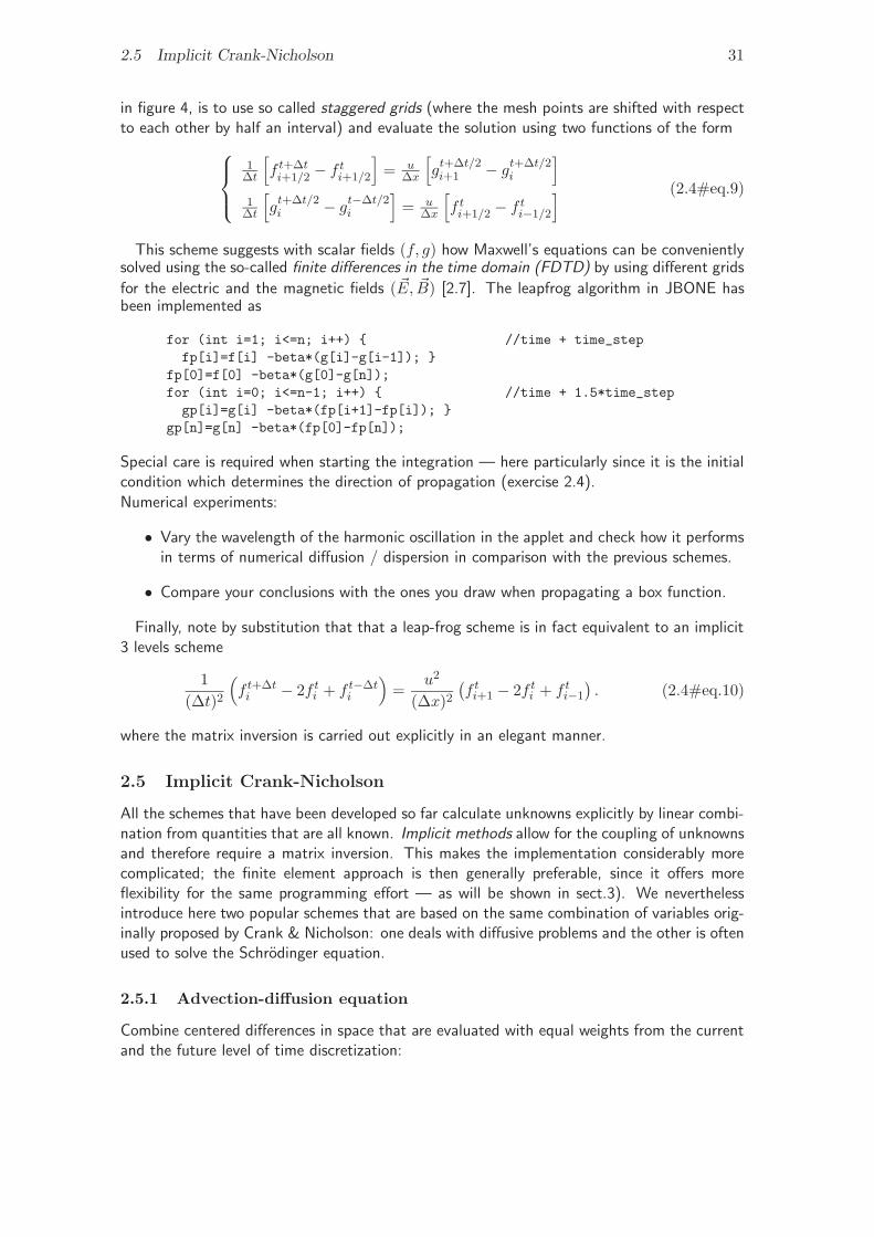
2.5 Implicit Crank-Nicholson
All the schemes that have been developed so far calculate unknowns explicitly by linear combi-nation from quantities that are all known. Implicit methods allow for the coupling of unknownsand therefore require a matrix inversion. This makes the implementation considerably morecomplicated; the finite element approach is then generally preferable, since it offers moreflexibility for the same programming effort — as will be shown in sect.3). We neverthelessintroduce here two popular schemes that are based on the same combination of variables orig-inally proposed by Crank & Nicholson: one deals with diffusive problems and the other is oftenused to solve the Schrodinger equation.
2.5.1 Advection-diffusion equation
Combine centered differences in space that are evaluated with equal weights from the currentand the future level of time discretization:
32 2 FINITE DIFFERENCES
∆t + t
t
x
t
j−1 j j+1
Figure 5: Implicit Crank-Nicholson.
f t+∆tj − f tj
∆t+
u
2
f t+∆tj+1 − f t+∆t
j−1
2∆x+f tj+1 − f tj−1
2∆x
− D
2
f t+∆tj+1 − 2f t+∆t
j + f t+∆tj−1
∆x2+f tj+1 − 2f tj + f tj−1
∆x2
= 0
(2.5.1#eq.11)
This Crank-Nicholson scheme is conveniently written as a linear system −α/2− β/41 + α−α/2 + β/4
T
·
f t+∆tj−1
f t+∆tj
f t+∆tj+1
=
α/2 + β/41− α
α/2− β/4
T
·
f tj−1
f tjf tj+1
(2.5.1#eq.12)
showing explicitly the tri-diagonal structure of the matrix implemented in JBONE as
BandMatrix a = new BandMatrix(3, f.length);BandMatrix b = new BandMatrix(3, f.length);double[] c = new double[f.length];for (int i=0; i<=n; i++) a.setL(i,-0.25*beta -0.5*alpha); //Matrix elementsa.setD(i, 1. +alpha);a.setR(i, 0.25*beta -0.5*alpha);b.setL(i, 0.25*beta +0.5*alpha); //Right hand sideb.setD(i, 1. -alpha);b.setR(i,-0.25*beta +0.5*alpha);
c=b.dot(f); //Right hand sidec[0]=c[0]+b.getL(0)*f[n]; // with periodicityc[n]=c[n]+b.getR(n)*f[0];
fp=a.solve3(c); //Solve linear problem
We will show later in sect.3 how the simple BandMatrix.solve3() method solves the linearsystem efficiently with an LU-factorisation in O(N) operations [2.7] dealing explicitly with theperiodicity.
Repeating the von Neumann stability analysis with (2.5.1#eq.11), a pure diffusive process(u = α = 0) yields the amplification factor
G =1− 2α sin2
(k∆x
2
)1 + 2α sin2
(k∆x
2
) (2.5.1#eq.13)
proving that this scheme is unconditionally stable ∀∆x, ∀∆t, phase errors affecting shortwavelength oscillations k∆x ∼ 1. The analogue is true also for the advective part. This
2.5 Implicit Crank-Nicholson 33
favorable stability property can nicely be exploited when solving diffusion dominated problemsthat concerned mainly with the evolution of large scale features λ ∆x.
Starting from a relatively smooth Gaussian pulse that is subject both to advection anddiffusion u = D = 1, the document on-line shows that a reasonably accurate solution (12 %for the valley to peak ratio as the time reaches 100) can be computed using extremely largetime steps with α = β = 5.Numerical experiments:
• Repeat the calculation with an initial box function; what happens?
• Add a few tiny time steps using a 2 level scheme (2.1#eq.1) at the end of an implicitevolution with very large time steps. When is this combination particularly indicated?
2.5.2 Schrodinger equation
When a complex wave function |ψ >= ψ(x, t) (which represents a non-decaying particle inquantum mechanics) evolves in time, the physical problem requires that the total probabilityof finding that particle somewhere in space remains exactly unity at all times < ψ|ψ >=∫|ψ|2dx = 1 ∀t. Solving the Schrodinger equation
i∂ψ
∂t= H(x)ψ with H(x) = − ∂2
∂x2+ V (x) (2.5.2#eq.14)
here normalized so as to have Planck’s constant ~ = 1, the particle mass m = 1/2 and a staticpotential V (x), it could therefore be important to keep the evolution operator unitary even in itsdiscretized form. This is achieved by writing the formal solution ψ(x, t) = exp(−iHt)ψ(x, 0)in the so-called Cayley form for the finite difference in time
exp(−iH∆t) '1− i
2H∆t1 + i
2H∆t(2.5.2#eq.15)
This approximation is unitary, accurate to second-order in time O(∆t2) and suggests an evo-lution of the form
(1 +i
2H∆t)ψt+∆t = (1− i
2H∆t)ψt (2.5.2#eq.16)
Replacing the second order derivative in the Hamiltonian operator H(x) with finite differencescentered in space O(∆x2), one obtains a scheme that is stable, unitary and in fact again theCrank-Nicholson method in a new context:
ψt+∆tj +
i∆t2
(−ψt+∆tj−1 − 2ψt+∆t
j + ψt+∆tj+1
∆x2+ Vjψ
t+∆tj
)=
= ψtj +i∆t2
(−ψtj−1 − 2ψtj + ψtj+1
∆x2+ Vjψ
tj
)(2.5.2#eq.17)
The scheme is finally cast into the linear system − i∆t2∆x2
1 + i∆t∆x2 + i∆t
2 Vj− i∆t
2∆x2
T
·
ψt+∆tj−1
ψt+∆tj
ψt+∆tj+1
=
i∆t2∆x2
1− i∆t∆x2 − i∆t
2 Vji∆t
2∆x2
T
·
ψtj−1
ψtjψtj+1
(2.5.2#eq.18)
exploiting the tri-diagonal structure of the matrix, and has been implemented in JBONE usingcomplex arithmetic
34 2 FINITE DIFFERENCES
BandMatrixC a = new BandMatrixC(3, h.length); //Complex objectsBandMatrixC b = new BandMatrixC(3, h.length);Complex[] c = new Complex[h.length];Complex z = new Complex();
double[] V = physData.getPotential(); //Heavyside(x-L/2) timesdouble scale = 10.*velocity; // an arb. scaling factordouble dtodx2 = timeStep/(dx[0]*dx[0]);Complex pih = new Complex(0., 0.5*dtodx2);Complex mih = new Complex(0.,-0.5*dtodx2);Complex pip1 = new Complex(1., dtodx2);Complex mip1 = new Complex(1., -dtodx2);
for (int i=0; i<=n; i++) z = new Complex(0.,0.5*scale*timeStep*V[i]);a.setL(i,mih); //Matrix elementsa.setD(i,pip1.add(z));a.setR(i,mih);b.setL(i,pih); //Right hand sideb.setD(i,mip1.sub(z));b.setR(i,pih);
c=b.dot(h); //Right hand side withc[0]=c[0].add(b.getL(0).mul(h[n])); // with periodicityc[n]=c[n].add(b.getR(n).mul(h[0]));
hp=a.solve3(c); //Solve linear problem
for (int i=0; i<=n; i++) //Plot norm & real partfp[i]=hp[i].norm();gp[i]=hp[i].re();
It again relys on the complex BandMatrixC.solve3() method to solve the linear system effi-ciently with a standard LU-factorisation with O(N) complex operations [2.7].
The document on-line shows the evolution of the wavefunction and the probability when awavepacket is scattered on a (periodic) square potential barrier rizing in the right side of thesimulation domain. The conservation of the moment shows that the total probability remainsindeed perfectly conserved for all times.
Numerical experiment:
• Modify the energy in the wavepacket ICWavelength and verify that the applet recpro-duces the probability of reflection / transmission accross a potential barrier.
2.6 Exercises
2.1 Upwind differences, boundary conditions
Use upwind differences and modify the explicit 2 level scheme (2.1#eq.1) in JBONE to proposea new scheme that is stable both for forward and backward propagation. Implement Dirichletconditions to maintain a constant value on the boundary up-the-wind (i.e. in the back of thepulse) and an outgoing wave in the front.
2.6 Exercises 35
2.2 Numerical dispersion
Determine analytically how the explicit 3 levels scheme (2.2#eq.5) affects the advection ofshort wavelength components and calculate the growth rate of the numerical instability whenD 6= 0. Use a harmonic initial condition to confirm your results with the JBONE applet.
2.3 Shock waves using Lax-Wendroff
Follow the Lax-Wendroff approach to solve the Burger equation (1.3.4#eq.2) with the JBONEapplet. Implement a first order scheme and study the numerical convergence for different valuesof the physical diffusion D. If you want, you may try to go to second order and notice that it isbetter not to expand high order non-linear derivatives to keep 2f(∂xf)2 + f2∂2
xf = (∂2xf
3)/3.How can you compare the performance of the first and second order schemes? Hint: usethe high order finite differences formulas (1.4.2#eq.2) to calculate an approximation for thederivatives.
2.4 Leapfrog resonator
Study the intitialization of the leapfrog scheme (2.4#eq.9) in the JBONE applet and examinehow you can affect the direction of propagation of a Gaussian pulse (comment out one ofthe three definitions for gm). Modify the numerical scheme to incorporate perfectly reflectingboundary conditions.
2.5 European option
Use a finite difference schemes to solve the Black-Scholes equation
∂V
∂t+
12σ2S2∂
2V
∂S2+ (r −D0)S
∂V
∂S− rV = 0 (2.6#eq.1)
for the value of a European Vanilla put option using an underlying asset S ∈ [0; 130] and astike price E = 95, a fixed annual interest rate r = 0.05, a volatility σ = 0.7155, no dividendD0 = 0 and T = 0.268 year to expiry. Start with a change of variables t = T − t′ to form abackward-parabolic equation in time and propose an explicit scheme for the variables (S, t′).
After giving some thoughts to the numerical stability of this solution, examine the transfor-mation into normalized variables (x, τ) defined by t = T − 2τ/σ2, S = E exp(x) and use theansatz
V (S, t) = E exp[−1
2(k2 − 1)x−
(14
(k2 − 1)2x+ k1
)τ
]u(x, τ) (2.6#eq.2)
k1 = 2r/σ2, k2 = 2(r −D0)/σ2
to reduce the original Black-Scholes equation to a standard diffusion problem
∂u
∂τ− ∂2u
∂x2= 0 (2.6#eq.3)
Derive initial and boundary conditions and implement the improved scheme in the JBONEapplet. Compare with the Monte-Carlo solution previously developed in this course now runningvery nicely as an applet
36 2 FINITE DIFFERENCES
2.6 Particle in a periodic potential
The quantum mechanics for particles in a periodic potential is a cornerstone of Solid StatePhysics (see e.g. Ashcroft and Mermin [13], chapters 8 and 9).
It is shown from perturbative theory that the addidtion of a weak periodic potential modifiesthe energy levels of the particle as compared to the free particle case E = h2k2/2m. Themost dramatic effect is felt for wavenumbers k close to a Bragg plane, for which a forbiddengap in allowed energy occurs. If L is the periodicity of the potential, K = 2p/L is called areciprocal lattice vector, and the Bragg plane is at k = K/2. Thus the dispersion relation forparticles in a weak potential is such that the group velocity vanishes at the Bragg plane.
The aim of this exercise is to demonstrate this property. Modify the scheme for theSchroedinger equation (2.5.2#eq.18) to include a periodic potential. Choose the period lengthfor the potential and an amplitude set by PhysDataValue. See how plane wave particlespropagate when their wavelength is equal to the Bragg condition, as compared to when theirwavelength differs from that. Then choose a wave packet. Document your observations andrelate them to the theory.
2.7 Further Reading
• Eulerian schemes for advection-diffusion problems.Numerical Recipes [4] §19.1–19.2, Boris [14]
• FDTD leapfrog for Maxwell’s equation.Jin [15], EMLIB homepage12 [16]
• Direct and iterative methods for solving linear systems.Numerical Recipes [4] §2.4, Dahlquist [6] §6.3, §11.1–11.4, Saad [17]
• Option pricing.Wilmott [18], Bjork [19], Duffie [20], Rebonato [21]
2.8 Solutions
2.5. Option pricing. It is really not possible to give here a complete introduction into thebroad subject of option pricing; simple explanations can be found on-line in a tutorial bythe Chicago Bord of Exchange13; a more thorough analysis is given in books by Wilmott[18] and Rebonato [21]. For this excercise, it is sufficient to understand that an EuropeanVanilla put option is a contract giving its owner the right to sell a certain asset (calledthe underlying) for a fixed price (E the exercise or strike price) at a prescribed time Tin the future (the expiry date).
The parameters of the exercise have been chosen for the underlying QQQ index (NAS-DAQ top 100) on the evening of May 24, 2000 when QQQ was traded for S = 79.5 USD(alternatively, you can take the value from today and repeat the exercise with updatedvalues). Imagine you are the owner of a put option allowing you to sell a QQQ share forE = 95.00 USD on September 1st, 2000: you may want to know how much this rightwas worth on May 24, 2000, i.e. T = 0.268 year before expiry (alt. take today).
12http://emlib.jpl.nasa.gov/13http://www.cboe.com
2.8 Solutions 37
At expiry on September 1st, 2000, it is clear that the value of the put depends onlyon the price S of the underlying share and is given by the payoff function P (S, t =0) = max(E − S, 0) given as initial condition to the JBONE applet: the put option isworthless if QQQ is traded above S = 95 USD (an option is a right you are allowed notto exercise) and you will earn the price difference if QQQ is traded below (you can buyQQQ shares for e.g. S = 75 USD on the market and sell them without taking any riskfor the strike price of E = 95 USD with a net profit of 20 USD per share).
Two factors at least can change the price of this right from May to September:
1. If you give your money to a bank, you can earn an interest rate of say r = 0.05 onyour deposit; you should therefore discount this systematic (risk free) return fromthe value of the option during the entire period your money is invested.
2. The market (and in particular NASDAQ) is volatile. Prices change constantly withwhat may be modeled as a random component in the price of a share: even ifchance are slim, you may still earn money with a put option at 95 USD if QQQis above 100 USD in August... if the market crashes, making you rich! Clearly,options keep a finite value until they expire depending on the underlying volatility14.For QQQ, this was σ = 0.7155 in May (alt. take the value today).
The Black & Scholes model takes these factors into account and integrates the payofffunction backwards in time to model the price of an option before it expires.
Using an explicit 2 levels spatially centered finite difference scheme, eq.2.6#eq.1 cannaively be written as
V t+∆t = V t + ∆t[σ2(
12j∆S)2Vj+1 − 2Vj + Vj−1
∆S2+ r(j∆S)
Vj+1 − Vj−1
2∆S− rVj
]= 0
(2.8#eq.1)
and cast into
V t+∆t =∆t2
(σ2j2 + rj)Vj+1 + (1− σ2j2∆t+ r∆t)Vj +∆t2
(σ2j2 − rj)Vj−1
(2.8#eq.2)
This has been implemented in JBONE as:
double E = runData.getInitialShapePosition(); //Exercise pricedouble sigmaSq= diffusCo; //Volatility squaredouble rate = velocity; //Interest rate
fp[0]=E*Math.exp(-rate*time); //Boundary conditionfor (int i=1; i<n; i++) fp[i]=f[i+1]* 0.5*timeStep*(sigmaSq*i*i +rate*i) //Explicit 2 levels
+f[i ]*(1.0-timeStep*(sigmaSq*i*i +rate ))+f[i-1]* 0.5*timeStep*(sigmaSq*i*i -rate*i);
fp[n]=fp[n-1]+dx[0]*(fp[n-1]-fp[n-2]); //Boundary condition
Press Start/Stop to start the (slow) integration backward in time. Increase the timestep by a factor 2: after only about 40 steps, a numerical instability develops that canbe traced down to a violation of the stability criterion σ2∆t/∆x2 < 1/2 (eq.2.1#eq.4).
14http://www.cboe.com/tools/historical/vol0400.txt
38 2 FINITE DIFFERENCES
The problem with this naive approach is that the random changes in the asset pricesδS are in reality lognormally distributed, so that the natural mesh for the a randomwalk should in fact be equally spaced in logS rather than S. The time step is thereforelimited by the largest asset price, where the relative mesh intervals ∆S is smallest.
To avoid instabilities and negative values for large asset prices, it is possible to changefrom financial (S, t′) to lognormal variables (x, τ) and evolve the standard diffusionequation (eq.2.6#eq.3). An interpolation back to financial variable is only required fordiagnostic purposes. This has been implemented in JBONE as:
double E = runData.getInitialShapePosition(); //Exercise pricedouble sigmaSq= diffusCo; //Volatility squaredouble rate = velocity; //Interest ratedouble divid = disperCo; //Dividendint j;double x0, x1, f0, f1, xi; //Change variablesdouble tau = 0.5*sigmaSq*time; // f(x,t) ->double dtau= 0.5*sigmaSq*timeStep; // fm(xx,tau)double xx0 = Math.log(x[1]/E);double dxx =(Math.log(x[n]/E)-Math.log(x[1]/E))/(n-1);double k1 = 2*rate/sigmaSq;double k2 = 2*(rate-divid)/sigmaSq;double k2m1 = k2-1.;
//Interpolate from financial (x,t) to lognormal variables (xx,tau)if (time <=timeStep) j=1; ; x0=xx0;f0=f[1]/E*Math.exp(0.5*k2m1*x0+(0.25*k2m1*k2m1+k1)*tau);x1=x0; f1=f0; xi=x0;for (int i=1; i<n; i++) //Loop over lognormal mesh indexxi=xx0+(i-1)*dxx;while (xi>=x1) j++; x0=x1; f0=f1; x1=Math.log(x[j]/E); f1=f[j]/E*Math.exp(0.5*k2m1*x1+(0.25*k2m1*k2m1+k1)*tau);fm[i]= f0 + (xi-x0)*(f1-f0)/(x1-x0);
fm[n]= fm[n-1] + dxx*(fm[n-1]-fm[n-2]);
else //Retrieve fm[] from previous time step
//Solve diffusion equation with an explicit 2 levels schemedouble D = dtau/(dxx*dxx);for (int i=2; i<n; i++)f[i]= fm[i] + D*(fm[i+1]-2.*fm[i]+fm[i-1]);
f[1]= Math.exp(0.5*k2m1*xx0+0.25*k2m1*k2m1*tau); //Boundary cond.f[n]= f[n-1] + dxx*(f[n-1]-f[n-2]);
//Interpolate back from lognormal to financial mesh variablesfp[0]=E*Math.exp(-rate*time); //Analyticallyj=1; x0=x[0]; x1=x0; f0=fp[0];xi=xx0; f1=f[1]*E/Math.exp(0.5*k2m1*xi+(0.25*k2m1*k2m1+k1)*tau);for (int i=1; i<n; i++) //Loop over financial mesh indexwhile (x[i]>=x1)j++;x0=x1;f0=f1;xi=xx0+(j-1)*dxx;x1=E*Math.exp(xi);
f1=f[j]*E/Math.exp(0.5*k2m1*xi+(0.25*k2m1*k2m1+k1)*tau);
2.9 Interactive evaluation form 39
fp[i]= f0 + (x[i]-x0)/(x1-x0)*(f1-f0);xi=Math.log(x[n]/E);fp[n]=f[n]*E/Math.exp(0.5*k2m1*xi+(0.25*k2m1*k2m1+k1)*tau);
Using lognormal variables, the stability limit is the same for all prices; the maximum valuecan therefore be considerably larger and the problem with negative payoffs for large assetprices is cured. After the first step, you can clearly see the numerical interpolation errorinduced by changing to lognormal variables and back; higher precision is achieved byrefining the mesh, but keep in mind that the scheme remains subject to the stabilitycondition (eq.2.1#eq.4).
After these numerical considerations, you are ready to calculate what was the price ofyour put option on May 24, 2000 (alt. today).
1. Edit the value of the
• interest rate r → Velocity = 0.05,
• volatility square σ2 = 0.71552 = 0.512→ Diffusion = 0.512,
• time to expiry of 98 days = 0.268 year → Run time = 0.268
• strike price → ICPosition = 95.
• largest asset price → Mesh length = 130.
2. Press Initialize and then Start/Stop for the calculation
3. Select Data to java console in the applet top right selector, press Step 1 andswitch back to Double click to edit below
4. Open the java console (in Netscape, select Communicator->Tools->Java console)
With an underlying QQQ traded for S = 79.5 USD on the evening of May 24, 2000,the nearest grid point approximation from x[79]=80.23 shows that the price of the putoption will finally reach g[79]=14.77 on September 1st, but was still much higher onMay 24 f[79]=21.82 because of the so-called time value associated with the marketvolatility. This predicted value of 21.82 USD can finally be compared with the valueset by the market, which was 20.875 on the evening of May 24, 2000 (alt. consult thecurrent market price on the web). The agreement is certainly not bad given the crudeapproximations made for the input parameters... and remember: the Black-Scholes isonly a model of what the market really does!
2.9 Interactive evaluation form
Your anonymous opinion is precious. Please fill-in our anonymous form in the web edition.Thank you very much in advance for your collaboration!

40 2 FINITE DIFFERENCES
41
3 FINITE ELEMENTS METHODS
3.1 Mathematical background
To approximate a set of linear partial differential equations
L~v = ~r in Ω (3.1#eq.1)
for an unknown ~v ∈ V ⊂ Cn(Ω) continuously defined with n derivatives in the volume Ω andsubject to the boundary conditions
B~v = ~s in ∂Ω (3.1#eq.2)
a mathematician would probably first involve
Weighted residuals. Having defined a scalar product (·, ·) and a norm || · ||, the calculationessentially amounts to the minimization of a residual vector
||~R|| = ||~r − L~v|| (3.1#eq.3)
which can be carried out using tools from the variational calculus.
Variational form. A quadratic form is constructed for that purpose by choosing a testfunction ~w in a sub-space W that is “sufficiently general” and satisfies the boundaryconditions. The linear equation (3.1#eq.1) can then be written as an equivalent varia-tional problem
(~w, ~R) = (~w,L~v − ~r) = 0 ~v ∈ V, ∀~w ∈ W (3.1#eq.4)
Integration by parts. If ~w is differentiable at least once W ⊂ C1(Ω), the regularity re-quired by the forth-coming discretization can often be relaxed by partial integrations.Using L = ∇2 for illustration, Leibniz’ rule states that
∇ · (v ~w) = (∇v) · ~w + v∇ · ~w =⇒ ∇v · ~w = −v∇ · ~w +∇ · (v ~w) (3.1#eq.5)
Integrating over the volume Ω and using Gauss’ divergence theorem∫Ω∇ · ~F dV =
∫∂Ω
~F · ~dS
yields a generalized formula for partial integration:∫Ω∇v · ~w dV = −
∫Ωv∇ · ~w dV +
∫∂Ωv ~w · ~dS (3.1#eq.6)
For the special case where ~w = ∇u, this is known as Green’s formula∫Ωv∇2u dV = −
∫Ω∇v · ∇u dV −
∫∂Ωv∇u · ~dS (3.1#eq.7)
Note that the last (surface-) term can sometimes be imposed to zero (or to a finitevalue) when applying so-called natural boundary conditions.
42 3 FINITE ELEMENTS METHODS
Numerical approximation. It turns out that the formulation as a variational problem isgeneral enough that the solution ~v of (3.1#eq.4) remains a converging approximationof (3.1#eq.1) even when the sub-spaces V,W are restricted to finite, a priori non-orthogonal, but still complete sets V,W of functions; the overlap integrals betweenthese functions can then be handled simply as linear algebra by the computer.
In general, the discretized solution ~v is expanded in basis functions ~ej ∈ V ⊂ V whicheither reflect a property of the solution (e.g. the operator Green’s function in the Methodof Moments), or which are simple and localized enough so that they yields cheap innerproducts (~w, ~ej) and sparse linear systems (e.g. the roof-top function for the linear FiniteElement Method). Different discretizations are possible also for the test functions ~w.Among the most popular choices is the Galerkin method where test and basis functionsare both chosen from the same sub-space V ≡ W; the method of collocation consistsin taking ~w ∈ W = δ(~x − ~xj), j = 1, N which yields a point-wise evaluation of theintegrand on a discrete mesh ~xj, j = 1, N .
3.2 An engineer’s formulation
After a section of what a physicist believes might be a mathematician’s view of the subject,it is time for an example. Using the format of a “recipe” applicable to a rather broad class ofpractical problems, this shows how the advection-diffusion problem (1.3.2#eq.2) is formulatedusing Galerkin linear finite elements (FEMs) and how it is implemented in the JBONE applet.
Derive a weak variational form. “Multiply” your equation by ∀g ∈ C1(Ω),∫
Ω dx g∗(x)
where the conjugation is necessary only if your equation(s) is (are) complex:
∀g ∈ C1(Ω),∫ xR
xL
dx g
[∂f
∂t+ u
∂f
∂x−D∂
2f
∂x2
]= 0 (3.2#eq.1)
Integrate by parts. To avoid having to use quadratic basis functions for the discretizationof the second order diffusion operator, you now integrate by parts:∫ xR
xL
dx
[g∂f
∂t+ ug
∂f
∂x+D
∂g
∂x
∂f
∂x
]− Dg
∂f
∂x
∣∣∣∣xRxL
= 0 ∀g (3.2#eq.2)
Assuming a periodic domain, the surface term can here be cancelled, imposing so-callednatural boundary conditions.
Discretize time. This can be formulated in general using a partially implicit scheme f =(1− θ)f t + θf t+∆t, where θ ∈ [1/2; 1]:∫ xR
xL
dx
[g
(f t+∆t − f t
∆t
)+ ug
∂
∂x
[(1− θ)f t + θf t+∆t
]+D
∂g
∂x
∂
∂x
[(1− θ)f t + θf t+∆t
]]= 0
∫ xR
xL
dx
[g
∆t+ θug
∂
∂x+ θD
∂g
∂x
∂
∂x
]f t+∆t =
∫ xR
xL
dx
[g
∆t− (1−θ)ug ∂
∂x− (1−θ)D∂g
∂x
∂
∂x
]f t
(3.2#eq.3)
∀g, where all the unknowns have been reassembled on the left. Re-scale by ∆t, and
3.3 Numerical quadrature and solution 43
Discretize space using a linear FEMs expansion and a Galerkin choice for the test function:
f t(x) =N∑j=1
f tjej(x), ∀g ∈ ei(x), i = 1, N (3.2#eq.4)
∫ xR
xL
dx
ei N∑j=1
f t+∆tj ej + ∆tθeiu
N∑j=1
f t+∆tj
∂ej∂x
+ ∆tθD∂ei∂x
N∑j=1
f t+∆tj
∂ej∂x
=
∫ xR
xL
dx
ei N∑j=1
f tjej + ∆t(θ − 1)eiuN∑j=1
f tj∂ej∂x
+ ∆t(θ − 1)D∂ei∂x
N∑j=1
f tj∂ej∂x
∀i = 1, N (3.2#eq.5)
Note how the condition ∀g ∈ C1([xL;xR]) is now used to create as many independentequations i = 1, N as there are unknowns f t+∆t
j , j = 1, N . All the essential boundaryconditions are imposed by allowing e1(x) and eN (x) to overlap in the periodic domain.Since only the basis and test functions ei(x), ej(x) and perhaps the problem coefficientsu(x), D(x) remain space dependent, the discretized equations can all be written interms of inner products for example of the form (ei, ue′j) =
∫ xRxLdx u(x)ei(x)e′j(x).
Reassembling them in matrix notation,
Write a linear system through which the unknown values from the next time step f t+∆tj
can implicitly be calculated in terms of the current values f tj
N∑j=1
Aijft+∆tj =
N∑j=1
Bijftj (3.2#eq.6)
To relate this Galerkin linear FEM scheme with the code which has been implemented inthe JBONE applet, it is necessary now to evaluate the integrals from the inner product; thisis usually performed with a numerical quadrature.
3.3 Numerical quadrature and solution
Except when the PDE coefficients are singular and require a special treatment, the precisionrequired for the numerical integration really depends on the type of FEMs; in general, it issufficient to preserve the convergence rate guaranteed by the discretization. Using a numericalquadrature of the form∫ b
af(y)dy =
b− a2
n∑i=1
wif(yi) +Rn (3.3#eq.1)
yi =(b− a
2
)xi +
(b+ a
2
)(3.3#eq.2)
with the abscissas xi, weights wi and rests Rn given in the table 1 below it is possible exactlyintegrate polynomials with a degree (p − 1), simply by superposing n terms for which theintegrand is evaluated at the specified location yi(xi) ∈ [a; b] and weighted by the factor wi.Using the powerful Gaussian quadrature, the product of two cubic FEMs will therefore require
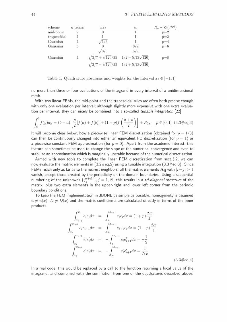
44 3 FINITE ELEMENTS METHODS
scheme n terms ±xi wi Rn ∼ O(f (p))mid-point 2 0 1 p=2trapezoidal 2 1 1 p=2Gaussian 2
√1/3 1 p=4
Gaussian 3 0 8/9 p=6√3/5 5/9
Gaussian 4√
3/7 +√
120/35 1/2− 5/(3√
120) p=8√3/7−
√120/35 1/2 + 5/(3
√120)
Table 1: Quadrature abscissas and weights for the interval xi ∈ [−1; 1]
no more than three or four evaluations of the integrand in every interval of a unidimensionalmesh.
With two linear FEMs, the mid-point and the trapezoidal rules are often both precise enoughwith only one evaluation per interval; although slightly more expensive with one extra evalua-tion per interval, they can nicely be combined into a so-called tunable integration [22]∫ b
af(y)dy = (b− a)
[p
2[f(a) + f(b)] + (1− p)f
(a+ b
2
)]+R2, p ∈ [0; 1] (3.3#eq.3)
It will become clear below, how a piecewise linear FEM discretization (obtained for p = 1/3)can then be continuously changed into either an equivalent FD discretization (for p = 1) ora piecewise constant FEM approximation (for p = 0). Apart from the academic interest, thisfeature can sometimes be used to change the slope of the numerical convergence and even tostabilize an approximation which is marginally unstable because of the numerical discretization.
Armed with new tools to complete the linear FEM discretization from sect.3.2, we cannow evaluate the matrix elements in (3.2#eq.5) using a tunable integration (3.3#eq.3). SinceFEMs reach only as far as to the nearest neighbors, all the matrix elements Aij with |i−j| > 1vanish, except those created by the periodicity on the domain boundaries. Using a sequentialnumbering of the unknowns f t+∆t
j , j = 1, N , this results in a tri-diagonal structure of thematrix, plus two extra elements in the upper-right and lower left corner from the periodicboundary conditions.
To keep the FEM implementation in JBONE as simple as possible, homogeneity is assumedu 6= u(x), D 6= D(x) and the matrix coefficients are calculated directly in terms of the innerproducts ∫ xi
xi−1
eieidx =∫ xi+1
xi
eieidx = (1 + p)∆x4∫ xi+1
xi
eiei+1dx =∫ xi+1
xi
ei+1eidx = (1− p)∆x4∫ xi+1
xi
eie′idx = −
∫ xi+1
xi
eie′i+1dx = −1
2∫ xi+1
xi
e′ie′idx = −
∫ xi+1
xi
e′ie′i+1dx =
1∆x
(3.3#eq.4)
In a real code, this would be replaced by a call to the function returning a local value of theintegrand, and combined with the summation from one of the quadratures described above.
3.3 Numerical quadrature and solution 45
Substituting back into (3.2#eq.5) finally yields the FEM scheme (1− p)∆x4 − θ∆t
u2 − θ∆t
D∆x
(1 + p)2∆x4 + θ∆t 2D
∆x
(1− p)∆x4 + θ∆tu2 − θ∆t
D∆x
T
·
f t+∆ti−1
f t+∆ti
f t+∆ti+1
=
(1− p)∆x4 − (θ − 1)∆tu2 − (θ − 1)∆t D∆x
(1 + p)2∆x4 + (θ − 1)∆t 2D
∆x
(1− p)∆x4 + (θ − 1)∆tu2 − (θ − 1)∆t D∆x
T
·
f ti−1
f tif ti+1
(3.3#eq.5)
After initialization where the initial condition is discretized with trivial projection on piecewiselinear “roof-top” FEMs, the scheme is implemented in JBONE using two tri-diagonal matrixesa, b and a vector c:
BandMatrix a = new BandMatrix(3, f.length);BandMatrix b = new BandMatrix(3, f.length);double[] c = new double[f.length];
double h = dx[0];double htm = h*(1-tune)/4;double htp = h*(1+tune)/4;
for (int i=0; i<=n; i++) a.setL(i, htm +h*(-0.5*beta -alpha)* theta );a.setD(i,2*(htp +h*( alpha)* theta ));a.setR(i, htm +h*( 0.5*beta -alpha)* theta );b.setL(i, htm +h*(-0.5*beta -alpha)*(theta-1) );b.setD(i,2*(htp +h*( alpha)*(theta-1)));b.setR(i, htm +h*( 0.5*beta -alpha)*(theta-1) );
c=b.dot(f); //Right hand sidec[0]=c[0]+b.getL(0)*f[n]; // with periodicityc[n]=c[n]+b.getR(n)*f[0];
fp=a.solve3(c); //Solve linear problem
The BandMatrix.solve3() method is again used to compute a direct solution in O(N) opera-tions with LU-factorization. The on-line document illustrates the advection of a box, calculatedwith a piecewise linear “roof-top” FEMs discretization (p = 1/3) slightly decentered in time(θ = 0.55).
After a considerable effort spent in understanding this FEM discretization, isn’t it frustratingto see how similar the code is with the implicit Crank-Nicholson FD scheme from sect.2.5?This should be the main argument for the community who still uses implicit finite differenceschemes! With some thinking but the same computational cost, a finite element approachoffers considerably more flexibility: it is now for example easy to densify the mesh15, varythe partially implicit time integration from centered to fully implicit θ ∈ [1
2 ; 1] and tune theintegration p ∈ [0; 1]. Convince yourself that Crank-Nicholson (2.5.1#eq.12) and this FEMscheme (3.3#eq.5) are strictly equivalent for a homogeneous mesh xj = j∆x, j = 1, N , atime centered integration θ = 1
2 and a trapezoidal quadrature p = 1. Also take a coupleof minute to experiment how you can affect the numerical dispersion / diffusion of shortwavelengths by varying both the parameters θ ∈ [1
2 ; 1] and p ∈ [0; 1].15Although this has, for pedagogical reasons, here not been exploited
46 3 FINITE ELEMENTS METHODS
Numerical experiments:
• Vary the TimeImplicit and TuneIntegr parameters and determine which combinationsyields the smallest numerical damping. Do your conclusions depend on the CFL number?
• Repeat this study to minimize the phase errors
3.4 Linear solvers
Writing efficient solvers for linear systems is a complete chapter of numerical analysis — andinvolves much more than what can be introduced here with a couple of sentences! As a userof software libraries such as Netlib [23] or PetSc [24], it is however sufficient to have a roughidea of what type of solvers exist and what they do.
Direct LU factorization. Remember that you should a priori never calculate a matrixinverse; you can solve a linear problem directly with only a third of the operations bydecomposing it first into lower and upper triangular parts [3.7] with 2
3N3 operations
(∗,+)
A · x = (L ·U) · x = L(U · x) = b (3.4#eq.1)
and then solve a forward-backward substitution with 2N2 operations
y1 =b1L11
; yi =1Lii
bi − i−1∑j=1
Lijyi
, i = 2, ...N
xN =yNU11
; xi =1Uii
yi − N∑j=i+1
Uijxj
, j = N−1, ...1 (3.4#eq.2)
A particularly simple version has been implemented in JBONE for tri-diagonal matri-ces, where the solve3() method computes the solution in O(N) operations; the firstand the last equations are simply eliminated “by hand” to take care of the periodic-ity. Many different implementations of one and the same algorithm exist and adapt theLU-factorization to specific non-zero patterns of A; it is likely that Netlib has a routinealready tailored for your application.
For matrices with more than three diagonals, it is important to allow for a pivoting duringthe factorization process — interchanging rows and columns to avoid divisions by smallvalues created on the diagonal. For particularly large problems, note the possibility ofstoring most of the matrix on disk with a frontal implementation of the same algorithm.
If memory consumption, calculation time or the parallelization of a solver becomes an issuefor 2D, 3D or even higher dimensions, it might be useful to consider iterative methods as analternative to direct solvers. The idea behind them is best understood from a splitting of thematrix into a sum16 of a diagonal D and strict lower −E and upper −F triangular parts
A = D−E− F (3.4#eq.3)
16Don’t get confused here with the product previously used for the LU factorization!

3.4 Linear solvers 47
An iterative solution of the problem
(b−A · xk+1)i = 0 , i = 1, ...N (3.4#eq.4)
is then sought where xk+1 =(ξ
(k+1)i
)is the (k + 1)-th iterate approximating the solution,
with components ranging from i = 1, ...N .
Iterative Jacobi. The simplest form of iteration consists in inverting only the diagonal
aiiξ(k+1)i = βi −
∑i6=j
aijξ(k)j (3.4#eq.5)
which is equivalent in matrix notation to
D · xk+1 = (E + F) · xk + b (3.4#eq.6)
Starting from an arbitrary initial guess x0, simple elliptic problems will –albeit slowly–converge to a stationary point which is the solution of the linear problem.
Gauss-Seidel. As the equations i = 1, ...N are updated one after the other, it is in factpossible to immediately use the updated information available in an explicit forwardscheme
aiiξ(k+1)i +
∑j<i
aijξ(k+1)j = βi −
∑j>i
aijξ(k)j (3.4#eq.7)
or
(D−E) · xk+1 = F · xk + b (3.4#eq.8)
where the calculation is carried out with an equation index increasing from i = 1, ...N .The reverse is also possible and is called backward Gauss-Seidel
(D− F) · xk+1 = E · xk + b (3.4#eq.9)
Successive over-relaxation — SOR is obtained when either of the Gauss-Seidel itera-tions (3.4#eq.8 or 3.4#eq.9) is linearly combined with the value of the previous step
xk+1 = ωxGSk + (1− ω)xk (3.4#eq.10)
using the parameter ω ∈ [0; 1] for an under-relaxation or ω ∈ [1; 2] for an over-relaxation.A symmetric-SOR (SSOR) scheme can be obtained for the combination
(D− ωE) · xk+1/2 = [ωF + (1− ω)D] · xk + ωb(D− ωF) · xk+1 = [ωE + (1− ω)D] · xk+1/2 + ωb
(3.4#eq.11)
Preconditionning / approximate inverse. Realizing that all the methods above are ofthe form xk+1 = G ·xk +f where G = 1−M−1 ·A, the linear problem approximativelybe diagonalized with a preconditionning
M−1 ·A · x = M−1 · b (3.4#eq.12)
48 3 FINITE ELEMENTS METHODS
MJacobi = D MSOR =1ω
(D− ωE)
MGS = D−E MSSOR =1
ω(2− ω)(D− ωE) ·D−1 · (D− ωF)
(3.4#eq.13)
Note that a product s = M−1 · A · x for a given x can be calculated without everforming the inverse, first with a product r = A · x and then solving the linear systemM · s = r in sparse format.
All these variants of Gauss-Seidel are simple and work fairly well for reasonable sized (e.g.20× 20) elliptic problems, making the much more complicated multigrid approach attractiveonly for larger applications which have to be solved many times. Solving hyperbolic (wave-)problems and non-Hermitian operators iteratively is however more complicated and remainsa matter of research [15], [25]. Methods rely in general both on a suitable preconditionningand the rapid convergence of Krylov-space and minimal residual methods such as GMRES orTFQMR [3.7].
It is important finally to note that the matrix-vector multiplication to form iterates can beperformed in sparse format, i.e. using only those matrix elements which are different fromzero. This is why iterative methods can be much more economical than direct solvers whichfill the matrix during the LU factorization process — if they converge!
3.5 Variational inequalities
Consider the obstacle problem, which arises when an elastic string held fixed at both ends ispulled over a smooth object and you seek an equilibrium without a priori knowing where arethe regions of contact between the string and this object. Define a function S(x) ∈ C1(Ω) tomeasure the elevation of the string in the interval Ω = [xL;xR] and O(x) ∈ C1(Ω) to modelthe shape of this object. The obstacle problem amounts to finding S(x) from the conditions:
1. the string always remains above the obstacle S(x) ≥ O(x),
2. the string satisfies the equilibrium equation. Neglecting the inertia, this says that thestring has either zero curvature (straight line between the points of contact) or a negativecurvature S′′ ≤ 0 (line of contact – in other words, the obstacle can only push the stringup, not pull it down).
Here are two manners for solving such problems that involve inequalities:
Linear complementary formulation. Reassemble all the conditions in a form
AB = 0, A ≥ 0, B ≥ 0 (3.5#eq.1)
After discretization, assuming that A invertible and positive definite, the linear problem
(x− c)(Ax− b) = 0, Ax ≥ b, x ≥ c (3.5#eq.2)
can be solved with the so-called projected SOR method, replacing (3.4#eq.10) by
xk+1 = max[c, ωxGSk + (1− ω)xk] (3.5#eq.3)
and starting the iteration from an initial guess x0 ≥ c.
3.6 Exercises 49
For the obstacle problem, the string follows either a straight line above the obstacleS′′ = 0 or fits exactly the object S − O = 0, suggesting how the complementaryproblem
S′′(S −O) = 0 S −O ≥ 0 − S′′ ≥ 0 (3.5#eq.4)
can be discretized with finite differences and solved using the pojected SOR method(exercise 3.5).
Variational formulation. This second approach is paticularly well suited for a discretiza-tion with finite elements is and best illustrated directly with the example. Choose a testfunction ∀w ∈ V ∈ C1(Ω) that satisfies the same conditions as the solution (w− c) ≥ 0.Having already (S − c) ≥ 0 and −S′′ ≥ 0, write two inequalities∫ xR
xL
−S′′(w − c) ≥ 0∫ xR
xL
−S′′(S − c) ≥ 0
and substract them ∫ xR
xL
−S′′(w − S) ≥ 0 (3.5#eq.5)
The condition c now appears only implicitly through the fact that w and S are membersof the same sub-space V. After the usual integration by parts and a discretization withlinear FEMs, the linear problem can be solved with projected SOR (3.5#eq.3) iterations(exercises 3.5, 3.7).
3.6 Exercises
3.1 Quadrature
Calculate the integral∫ π
0 sin(x)dx for a piecewise linear FEM approximation with two intervals,comparing the analytical result both with the tunable integration scheme (3.3#eq.3) and atwo point Gaussian quadrature (3.3#eq.1) using the table 1 with m = 2.
3.2 Diffusion in a cylinder
Use a Galerkin linear FEM approximation to compute the diffusion of heat when a homogeneouscylinder of radius rc, a conduction capacity κ and a radially inhomogeneous initial temperatureT0(r) is kept isolated from the outside world. (Hint: solve the heat equation for the evolutionof the temperature T (r, t) in cylindrical geometry
∂T
∂t− κ1
r
∂
∂r
(r∂T
∂r
)= 0 (3.6#eq.1)
Formulate a variational problem, integrate by parts and impose natural boundary conditionsto guarantee a regular behavior of the solution in the limit r → 0. Choose either a 2-pointsGaussian or a trapezoidal quadrature and form a linear system of equations which you completewith boundary conditions on the cylinder surface r = rc. Implement the scheme in the JBONEapplet.
50 3 FINITE ELEMENTS METHODS
3.3 Mass lumping
Examine the possibility of “lumping the mass matrix”, a procedure invented by structuralengineers in the 1970’s where the mass matrix (Aij) in (3.2#eq.6) is artificially set to unityto obtain an explicit scheme in terms only of the stiffness matrix (Bij). Study the advectionproblem separately from the diffusion.
3.4 Iterative solver
Implement an iterative–SOR solver in JBONE and study the number of iterations required toachieve a 10−6 precision for different values of the diffusion coefficient and advection velocity.
3.5 Obstacle problem
Compute a numerical solution for the obstacle problem from sect.3.5. For simplicity, take anobstacle parametrized by O(x) = 1
2 − x2 and an elastic string S(x) attached to the edge ofthe solution interval S(−1) = S(1) = 0. Hint: you may call the BandMatrix.ssor3() solverdocumented in the JBONE tree.
3.6 Numerical dispersion
Use a local ansatz f(x, t) ∼ exp(−iωt)∑
j exp(ikxj)ej(x) to determine how a Galerkin dis-cretization based on linear FEMs affects the dispersion of a wave in the standard wave equation(1.3.1#eq.2). Plot the phase velocity as a function of the numerical resolution).
3.7 American option
Extending your knowledge from exercise 2.5, use a Galerkin linear FEM formulation to solvethe Black-Scholes equation for an American put option, which differs from the European inthat it can be exercised anytime until it expires:
∫ x+
x−
∂u
∂τ(φ− u) +
∂u
∂x
(∂φ
∂x− ∂u
∂x
)dx ≥ 0, ∀φ ∈ W, ∀τ ∈ [0;
12σ2T ] (3.6#eq.1)
Restrict φ ∈ W to a piecewise linear test function which remains larger than the transformedpayoff functions φ(x, τ) ≥ g(x, τ) for all x and τ
gput(x, τ) = exp[
14
(k2 − 1)2 + 4k1
]τ
max
0, exp
[12
(k2 − 1)x− 12
(k2 + 1)x]
gcall(x, τ) = exp[
14
(k2 − 1)2 + 4k1
]τ
max
0, exp
[12
(k2 + 1)x− 12
(k2 − 1)x]
(3.6#eq.2)
and satisfying the boundary conditions φ(x+, τ) = g(x+, τ), φ(x−, τ) = g(x−, τ), φ(x, 0) =g(x, 0). Implement the scheme in JBONE and compare with the solution previously obtainedfor the European put in exercise 2.5.

3.7 Further reading 51
3.7 Further reading
• Finite elements.Johnson [8], Fletcher [7], Saad [17] §2.3
• Quadrature.Abramowitz [2] §25.4.29 with table 25.4, Numerical Recipes [4] §4.5
• Linear solvers.Dahlquist [6] §6, Saad [17], Numerical Recipes [4] §2.4.Software from netlib17, and PetSc18,
3.8 Interactive evaluation form
Your anonymous opinion is precious. Please fill-in our anonymous form in the web edition.Thank you very much in advance for your collaboration!
17http://www.netlib.org18http://www.mcs.anl.gov/petsc

52 3 FINITE ELEMENTS METHODS
53
4 FOURIER TRANSFORM
4.1 Fast Fourier Transform (FFT) with the computer
As mentioned earlier in sect.1.4, it is largely thanks to the possibility of computing efficientlythe Fourier transformation in O(N logN) operations that FFT’s can be considered as a viablealternative to solve partial differential equations. And here again, it is sufficient to have onlya rough idea of the underlying process to efficiently use the routines from software libraries.Particularly for FFT’s, you should privilege vendors implementations which have in generalbeen optimized for the specific computer you are using. Since no library is available yet inJAVA, a couple of routines from Numerical Recipes [4] have been translated for JBONE
into the FFT.java class, making as little modification as possible to the original code, enablingyou to learn more about the algorithm directly from the book. The Complex.java class hasbeen imported to illustrate how rewarding it is to work with Netlib [23] libraries.
Remember that a complex function f(x) of period L = 2π/K can be represented with acomplex series
f(x) =∞∑
m=−∞cm exp(imKx), cm =
1L
∫ a+L
af(x) exp(−imKx)dx (4.1#eq.1)
On the other hand, you can use the cosine – sine form
f(x) =a0
2+∞∑m=1
[am cos(mKx) + bm sin(mKx)] (4.1#eq.2)
am =2L
∫ a+L
af(x) cos(mKx)dx (m ≥ 0), bm =
2L
∫ a+L
af(x) sin(mKx)dx (m ≥ 1)
(4.1#eq.3)
with the following relations that hold between the Fourier coefficients
c0 = 12a0, cm = 1
2(am − ibm), c−m = c∗m, m ≥ 1a0 = 2c0, am = cm + c−m, bm = i(cm − c−m), m ≥ 1
(4.1#eq.4)
and only if f(x) is real
a0 = 2c0, am = 2Re(cm), bm = −2Im(cm), cm = c∗−m, m ≥ 1 (4.1#eq.5)
This is almost how the transformation is implemented in FFT.java, except that
1. the number of modes is assumed to be an integer power of 2. The creation of anFFT-object from data sampled on a homogeneous mesh relies on the command
double f = new double[64];FFT myFTObject = new FFT(f, FFT.inXSpace);
where FFT.inXSpace chooses the original location of the variable myFTObject of typeFFT.
2. To avoid negative indices and relying on the periodicity f(x + L) = f(x), negativeharmonics (−m) are stored in wrap-around order after the positive components and areindexed by N/2−m. For a real function f(x) = [7 + 8 cos(2πx/64) + 4 sin(2πx/32) +3 cos(2πx/2)] sampled on a mesh xj = 0, 1, ...63 with a period L = 64, the call to
54 4 FOURIER TRANSFORM
Complex spectrum = new Complex[64];double periodicity=64.;spectrum = myFTObject.getFromKSpace(FFT.firstPart,periodicity);for (int m=0; m<N; m++)
System.out.println("spectrum["+m+"] = "+spectrum[m]);
will print the non-zero components
spectrum[0] = (7. +0.0i)spectrum[1] = (4. +0.0i) spectrum[63] = (4. +0.0i)spectrum[2] = (0. +2.0i) spectrum[62] = (0. -2.0i)spectrum[32]= (3. +0.0i)
It is easy to see that the shortest wavelength component [32] will always be real if f(x)was real, since sin(2πx/2) is sampled exactly for the multiples of π.
3. Relying on the linearity of the FFT, two real numbers are packed into one complexnumber and transformed for the cost of a single complex transformation by initializing
double f = new double[64];double g = new double[64];FFT myPair = new FFT(f,g, FFT.inXSpace);
This is the reason for the argument FFT.firstPart used here above, asking for thespectrum of only the first (and in this example the only) function.
Apart from the array index which starts with [0] in JAVA, the implementation is equivalentto the routines in Numerical Recipes [4] and indeed very similar to many computer vendors.
4.2 Linear equations.
Albeit slower for a single time-step than all the numerical schemes we have seen so far, anFFT can be used to compute the Fourier representation of the advection-diffusion problem(1.3.2#eq.2) and describe the evolution of each Fourier component fm separately
dfmdt
+ ikmufm + k2mDfm = 0, km =
2πmL
(4.2#eq.1)
This can be integrated analytically without any restriction on the size of the time-step; startingdirectly from the initial condition, this yields for every Fourier component
fm(t) = fm(0) exp[−(ikmu+ k2mD)t)] (4.2#eq.2)
After an initialization, where the initial condition is discretized by sampling on a regular meshand stored for subsequent transformation, the scheme implemented in JBONE reads:
int N = mesh_.size(); //A power of 2double boxLen = mesh_.size()*mesh_.interval(0); //Periodicitydouble k = 2*Math.PI/boxLen; //NotationComplex ik1 = new Complex( 0., k );Complex ik2 = new Complex(-k*k, 0. );
Complex advection = new Complex(ik1.scale(velocity)); //VariablesComplex diffusion = new Complex(ik2.scale(diffusCo));
4.3 Aliasing, filters and convolution. 55
Complex[] s0 = new Complex[f.length]; //FFT real to KSpaces0=keepFFT.getFromKSpace(FFT.firstPart,boxLen); // only once
s[0] = s0[0];for (int m=1; m<N/2+1; m++) //Propagate directlytotal= advection.scale((double)(m )); // from initialtotal=total.add(diffusion.scale((double)(m*m))); // contition
exp=(total.scale(timeStep*(double)(jbone.step))).exp();
s[m ] = s0[m].mul(exp); // s0 contains the ICs[N-m] = s[m].conj(); // f is real
FFT ffts = new FFT(s,FFT.inKSpace); //Initialize in Kspacef = ffts.getFromXSpacePart(FFT.firstPart,boxLen); //FFT real back for plot
If you are a careful reader, you should now wonder about the sign of the phase factor, whichis exactly the opposite from (4.2#eq.2); the reason is that the phase of the spatial harmonicsis exactly opposite to the one used in the FFT routine from Numerical Recipes [4]. Thismakes the scheme look like as if it evolves backwards in time. Also note that once the initialcondition has been transformed to K-space, subsequent transformations back to X-space areonly required for the plotting.
The on-line document illustrates the advection of a box calculated with the same time step∆t = 0.5 as previously. The Gibbs phenomenon (artifact from using harmonic functions forthe discretization discussed in sect.1.4.5) is clearly visible except when u∆t/∆x is an integer;don’t get fooled however by the plotting, which (for simplicity – but still incorrectly) missesparts of the oscillations visible in figure 1 by linear interpolation between the grid points.The power of the method is evident when taking larger time-steps: edit the parameter toTimeStep=64, add some diffusion Diffusion=0.3 and compare the solution obtained in onesingle step with the result computed using your favorite FD or FEM scheme from the previoussections19. This is very nice indeed, but remember that dealing with an inhomogeneousmedium u(x), D(x) or complicated boundary conditions are problematic in Fourier space.Numerical experiments:
• Switch to Finite Differences and Finite Elements to measure the quality of pre-vious schemes for Advection=1, Diffusion=0.5 by comparing the results with theexact solution obtained with the Fourier transform. Hint: re-select the method thathas just been used to re-scale the plot window and print the maximum at the end of theevolution.
• Initialize a Gaussian and determine the optimal numerical parameters (MeshPoints,TimeStep, TimeImplicit, TuneIntegr) for different schemes to achieve a 2% precisionin the final value of the peak.
4.3 Aliasing, filters and convolution.
One of the beauties when using Fourier transforms, is the ability to work with a spectrum ofmodes and act on each of the components individually with a filter. By sampling a functionover a period L with a finite number of values N = L/∆ where ∆ is the size of the sampling
19Don’t forget to reduce again the time-step!
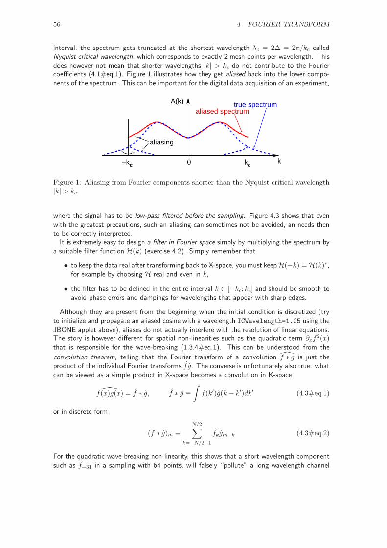
56 4 FOURIER TRANSFORM
interval, the spectrum gets truncated at the shortest wavelength λc = 2∆ = 2π/kc calledNyquist critical wavelength, which corresponds to exactly 2 mesh points per wavelength. Thisdoes however not mean that shorter wavelengths |k| > kc do not contribute to the Fouriercoefficients (4.1#eq.1). Figure 1 illustrates how they get aliased back into the lower compo-nents of the spectrum. This can be important for the digital data acquisition of an experiment,
0
aliasing
aliased spectrumtrue spectrum
k−kc c
A(k)
k
Figure 1: Aliasing from Fourier components shorter than the Nyquist critical wavelength|k| > kc.
where the signal has to be low-pass filtered before the sampling. Figure 4.3 shows that evenwith the greatest precautions, such an aliasing can sometimes not be avoided, an needs thento be correctly interpreted.
It is extremely easy to design a filter in Fourier space simply by multiplying the spectrum bya suitable filter function H(k) (exercise 4.2). Simply remember that
• to keep the data real after transforming back to X-space, you must keepH(−k) = H(k)∗,for example by choosing H real and even in k,
• the filter has to be defined in the entire interval k ∈ [−kc; kc] and should be smooth toavoid phase errors and dampings for wavelengths that appear with sharp edges.
Although they are present from the beginning when the initial condition is discretized (tryto initialize and propagate an aliased cosine with a wavelength ICWavelength=1.05 using theJBONE applet above), aliases do not actually interfere with the resolution of linear equations.The story is however different for spatial non-linearities such as the quadratic term ∂xf
2(x)that is responsible for the wave-breaking (1.3.4#eq.1). This can be understood from the
convolution theorem, telling that the Fourier transform of a convolution f ∗ g is just theproduct of the individual Fourier transforms f g. The converse is unfortunately also true: whatcan be viewed as a simple product in X-space becomes a convolution in K-space
f(x)g(x) = f ∗ g, f ∗ g ≡∫f(k′)g(k − k′)dk′ (4.3#eq.1)
or in discrete form
(f ∗ g)m ≡N/2∑
k=−N/2+1
fkgm−k (4.3#eq.2)
For the quadratic wave-breaking non-linearity, this shows that a short wavelength componentsuch as f+31 in a sampling with 64 points, will falsely “pollute” a long wavelength channel
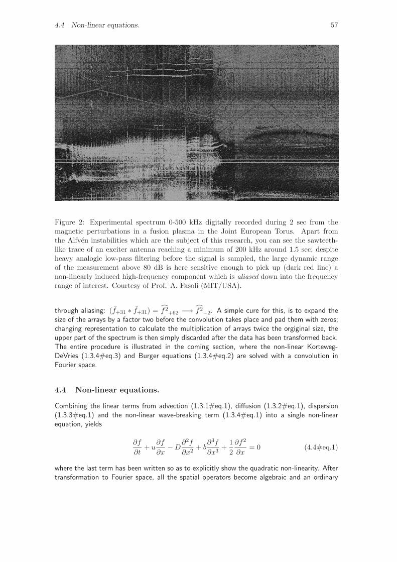
4.4 Non-linear equations. 57
Figure 2: Experimental spectrum 0-500 kHz digitally recorded during 2 sec from themagnetic perturbations in a fusion plasma in the Joint European Torus. Apart fromthe Alfven instabilities which are the subject of this research, you can see the sawteeth-like trace of an exciter antenna reaching a minimum of 200 kHz around 1.5 sec; despiteheavy analogic low-pass filtering before the signal is sampled, the large dynamic rangeof the measurement above 80 dB is here sensitive enough to pick up (dark red line) anon-linearly induced high-frequency component which is aliased down into the frequencyrange of interest. Courtesy of Prof. A. Fasoli (MIT/USA).
through aliasing: (f+31 ∗ f+31) = f2+62 −→ f2−2. A simple cure for this, is to expand the
size of the arrays by a factor two before the convolution takes place and pad them with zeros;changing representation to calculate the multiplication of arrays twice the orgiginal size, theupper part of the spectrum is then simply discarded after the data has been transformed back.The entire procedure is illustrated in the coming section, where the non-linear Korteweg-DeVries (1.3.4#eq.3) and Burger equations (1.3.4#eq.2) are solved with a convolution inFourier space.
4.4 Non-linear equations.
Combining the linear terms from advection (1.3.1#eq.1), diffusion (1.3.2#eq.1), dispersion(1.3.3#eq.1) and the non-linear wave-breaking term (1.3.4#eq.1) into a single non-linearequation, yields
∂f
∂t+ u
∂f
∂x−D∂
2f
∂x2+ b
∂3f
∂x3+
12∂f2
∂x= 0 (4.4#eq.1)
where the last term has been written so as to explicitly show the quadratic non-linearity. Aftertransformation to Fourier space, all the spatial operators become algebraic and an ordinary
58 4 FOURIER TRANSFORM
evolution equation is obtained for each individual Fourier component
dfmdt
+ (ikmu+ k2mD − ik3
mb)fm +12ikmf2
m = 0 (4.4#eq.2)
It would of course formally be possible to write the non-linear term as a convolution in K-space, but it is here much easier to write and efficient to compute the multiplication in X-space.Following the same lines as in sect.4.2, the linear terms are integrated analytically and yielda phase shift proportional to the time-step ∆t. The convolution is calculated numerically bytransforming back and forth from Fourier to configuration space, and after a simple Eulerintegration (1.2.1#eq.2) in time yields the formal solution
fmt+∆t
= fmtexp[−(ikmu+ k2
mD − ik3mb)∆t] +
∆t2ikmf2
m
t(4.4#eq.3)
This has been implemented in JBONE using the variable keepFFT to store the current values
of spectrum fmt
and the variable toolFFT for the transformation to X-space required by theconvolution and the plotting. As mentionned earlier in sect.4.2, the sign of time in (4.4#eq.3)has been changed to stick to the definition of the phase factor used in Numerical Recipes [4].
int N = mesh_.size(); //A power of 2double boxLen = mesh_.size()*mesh_.interval(0); //Periodicitydouble k = 2*Math.PI/boxLen; //NotationComplex ik1 = new Complex( 0., k );Complex ik2 = new Complex(-k*k, 0. );Complex ik3 = new Complex( 0.,-k*k*k);
Complex advection = new Complex(ik1.scale(velocity)); //VariablesComplex diffusion = new Complex(ik2.scale(diffusCo));Complex dispersion= new Complex(ik3.scale(disperCo));
//----- Non-linear term: convolutions = keepFFT.getFromKSpace(FFT.bothParts,boxLen); //Current SpectrumtoolFFT = new FFT(s,s,FFT.inKSpace); // for convolution
if (scheme.equals(jbone.ALIASED)) //With-/out aliasing,sp = toolFFT.aliasedConvolution(boxLen); // use an FFT to
else //scheme.equals(jbone.EXPAND) // calculate product,sp = toolFFT.expandedConvolution(boxLen); // FFT back to KSpace
//----- Linear terms: complex terms in spectrum ss = keepFFT.getFromKSpace(FFT.bothParts,boxLen); //Current Spectrumlinear= s[0];sp[0]=linear;for (int m=1; m<=N/2; m++) total= advection.scale((double)(m ));total=total.add(diffusion.scale((double)(m*m)));total=total.add(dispersion.scale((double)(m*m*m)));exp=(total.scale(timeStep)).exp();linear = s[m].mul(exp);nonlin = sp[m].mul(ik1.scale(0.5*timeStep*(double)(m)));sp[m ] = linear.add(nonlin);if (m<N/2) sp[N-m] = sp[m].conj(); //For a real spectrum
4.5 Exercises 59
keepFFT = new FFT(sp,FFT.inKSpace); //Spectrum is completetoolFFT = new FFT(sp,FFT.inKSpace); //inv FFT for plottingf=toolFFT.getFromXSpacePart(FFT.firstPart,boxLen);
Depending on the scheme selector, the convolution is calculated either without precaution andis subject to aliasing, or by temporarily expanding the spectrum padding the upper part withzeros to cure the problem.
The on-line document shows the evolution obtained for the Korteweg-DeVries equation,when two solitons propagate and collide through the delicate balance between the non-linearwave-breaking and dispersion. Change the switch to Aliased Convolution and verify howthe aliasing pollutes the spectrum with short wavelengths that rapidly evolve into a non-linearinstability.
Replace the dispersion with a small amount of diffusion by setting Dispersion=0.0 andDiffusion=0.1; evolve a Gaussian into a shock front and verify how much less aliasing seemsto be an issue for the Burger equation (1.3.4#eq.2), when a diffusive process physically dampsthe short wavelengths... Remember however that the cascade of energy from one wavelengthto another is now affected by the aliasing and is much more delicate to diagnose!Numerical experiments:
• Go back to the KdV equation by setting Dispersion=0.5 and try to cure the aliasedscheme with a small amount of non-physical diffusion. Separate the short wavelengths(unphysical aliases) from the longuer wavelengths (physical) by reducing the ICAmplitude.Is such a solution attractive?
4.5 Exercises
4.1 Advection-diffusion
Propose an alternative scheme solving the linear advection-diffusion problem in Fourier space,evolving the solution with small steps in time ∆t.
4.2 Equivalent filter for Zabusky’s FD scheme
Study Zabusky’s finite difference scheme for the Korteweg-DeVries equation
f t+∆tj − f t−∆t
j
2∆t+
13[f tj+1 + f tj + f tj−1
] f tj+1 − f tj−1
2∆x+ b
f tj+2 − 2f tj+1 + 2f tj−1 − f tj−2
2∆x3= 0
(4.5#eq.1)
using JBONE with b = 1/2. Calculate the equivalent Fourier space filter that is impliedfor the linear terms when the calculation is performed in configuration space. Add this fil-ter to the Fourier scheme available in JBONE and check that after filtering, both the FDand FT methods indeed are similar. What remains different? Hint: Zabusky’s finite differ-ence scheme has already been implemented under this link and can be executed by selectingFinite differences, Explicit 3-level and KdV (solitons) in the applet selectors.Your task in this exercise is first to calculate and then to implement a filter function Hm,which emulates for each Fourier component f t+∆t
m = Hmf tm the evolution that results fromthe finite differencing of the linear terms.
60 4 FOURIER TRANSFORM
4.3 Prototype problems
Modify the parameters of the non-linear equation 4.4#eq.3 in Fourier space to develop abetter qualitative understanding of what are advection, diffusion, dispersion and wave-breaking.Choose a regime where you trust the numerical description and propose a combination ofparameters you believe is particularly interesting.
4.4 Intrinsic numerical diffusion
Use the exact solution of the advection-diffusion equation calculated with the Fourier method(4.2#eq.2) to measure the numerical damping Dnum in FD / FEM schemes with differentimplicit-time and tunable-integration parameters. Start with uphys = Dphys = 1 and, afterevolving a narrow Gaussian, measure the final peak amplitude max[f ](Dtot) for a decreasingvalue of the total diffusion Dtot = Dphys +Dnum. Calculate the intrinsic numerical dampingDnum from the saturation you observe for small values of the physical damping Dphys. Hint:in JBONE, re-select the method that has just been used to re-scale the plot window and printthe maximum of the solution.
4.6 Further Reading
• FFT algorithm.Numerical Recipes [4] §12
4.7 Interactive evaluation form
Your anonymous opinion is precious. Please fill-in our anonymous form in the web edition.Thank you very much in advance for your collaboration!
61
5 MONTE-CARLO METHODS
5.1 Monte Carlo integration
The name stems from the city which is famous for its casinos and suggests a method involvingrandom numbers. The most common use of Monte-Carlo methods (mcm) is the evaluation ofmulti dimensional integrals [4]. Consider first the approximation of an integral obtained withthe trapezoidal rule (3.3#eq.1) by sampling on a uniform mesh∫ b
af(ξ) dξ =
N−1∑i=0
f(xi)b− aN
+ O(
1N
), xi = a+
b− aN − 1
i (5.1#eq.1)
Instead, you could use a mesh where the positions xi are random numbers uniformly dis-tributed in the interval [a, b]. This suggests the Monte Carlo integration∫ b
af(ξ) dξ =
N∑i=1
f(xi)b− aN
+O(
1√N
), xi ∈ U(a, b) (5.1#eq.2)
The rate of convergence of this Monte-Carlo integration is lower than for the sampling ona uniform mesh (5.1#eq.1). The strength however appears for the evaluation of integrals inhigher dimensions d > 2, where the mcm error scales as N−1/2 irrespective of the number ofdimensions, instead of the O
(N−1/d
)obtained using a uniform mesh.
5.2 Stochastic theory
This section is intended as a very short introduction into the stochastic calculus that providesthe mathematical foundation behind the Monte Carlo method. Check Kloeden [26] and VanKampen [27] for complete courses on the subject!
Definition The expected or mean value E and the variance V are defined by
E [X](x) ,∫ ∞−∞
xfX(x) dx (5.2#eq.1)
V[X](x) , E [X](
(x− E [X] (x))2)
(5.2#eq.2)
=E [X](x2)− E2 [X] (x) (5.2#eq.3)
where fX(x) is the density distribution function of the stochastic variable X.
Definition N (µ, σ) refers to the set of Gaussian or normal distributed stochastic variableX with density distribution function
fX(x) =1
σ√
2πexp
[−(x− µ)2
2σ2
](5.2#eq.4)
where µ is the mean and σ2 is the variance.
Definition U(a, b) refers to the set of uniformly distributed random numbers in theinterval [a, b].
Definition A stochastic process Wt is called a Wiener process (or Brownian motion) intime t if and only if
62 5 MONTE-CARLO METHODS
1. Wt+∆t−Wt ∈ N (0,√
∆t), where N is the set of normal distributed random numbers.
2. E [WtdWt] = E [Wt]E [dWt], where E denotes expected value, dWt = Wt+∆t −Wt and∆t > 0, i.e. the Wiener increment dWt is independent of the past.
The distribution function of a Wiener increment Wt+∆t −Wt is essentially the same functionas the Green’s function of the diffusion equation (1.3.2#eq.3).
The differential calculus of stochastic processes, the so called Ito calculus, involves newproperties that are fundamentally different from the ordinary Riemann calculus. The reasoncan be tracked down to the preferred direction of time t in the Ito integral:
Definition The Ito integral is defined as the limit of an explicit (forward Euler) dis-cretization ∫ T
0b(Wt, t) dWt ≡
∑i
lim∆ti→0
b(Wti , ti)(Wti+∆ti −Wti) (5.2#eq.5)
for any sequence ti : ti ∈ [0, T ], ti+1 = ti + ∆ti. The circle, stands for Ito differentialand states that dWt is independent of b(Wt, t).
Note that an implicit discretization in (5.2#eq.5) would give a fundamentally different result.Now consider a property Yt that is a sum of ordinary Riemann integral and an Ito integral.
YT =∫ T
0v(Yt, t)dt+
∫ T
0b(Yt, t) dWt (5.2#eq.6)
Integrating over a infinitely short time interval we obtain the so called stochastic differentialequation
dYt = v(Yt, t)dt+ b(Yt, t) dWt (5.2#eq.7)
which reduces to an ordinary differential equation if b(Yt, t) = 0 in the absence of a stochasticcomponent in the evolution
dYtdt
= v(Yt, t) (5.2#eq.8)
5.3 Particle orbits
When using the Monte Carlo method to solve pdes, functions are discretized using quasiparticles and differential operators need to be reformulated in terms of particle motions. In(1.4.7#eq.1) a quasi-particle is defined by a weight wi, a position xi and a shape function Si.For simplicity, we assume here unit weights wi = 1 and point shaped particles Si(x) = δ(x)described by the Dirac pulse. The solution is computed from an ensemble of particle positionsxi(t), that are called the particle orbits.
A deterministic orbit is described by an ordinary differential equation for the position X(t)as a function of time t
dX(t)dt
= v(X(t), t) (5.3#eq.1)
or
dX(t) = v(X(t), t)dt (5.3#eq.2)
5.3 Particle orbits 63
This equation can be solved numerically using the methods discussed in section 1.2.1, with anexplicit or implicit discretization of time
X(t+ ∆t) = X(t) + v(X(t), t)∆t “explicit” (5.3#eq.3a)X(t+ ∆t) = X(t) + v (X(t+ ∆t), t+ ∆t) ∆t “implicit” (5.3#eq.3b)
For an ensemble of N particles with orbits xi(t), a particle density distribution function f(x, t)is constructed according to section 1.4 and yields
f(x, t) =N∑i=0
δ(x− xi(t)) (5.3#eq.4)
Note that the first order moment is perfectly conserved, since no particle is lost.Using a large number of particles, the density distribution function is then approximated by
a smooth function. If the individual particle orbits X(t) evolve according to
dX(t) = v(X(t), t)dt. (5.3#eq.5)
then the Taylor’s transport theorem states that the evolution of particle density distri-bution function f(x, t) is described by the advection equation
∂f
∂t+
∂
∂x(vf) = 0 (5.3#eq.6)
This theorem makes it possible to study a PDE instead of an N -particle system; the reverseis also possible and used in particle methods involving the advection equation.
Let us now introduce the concept of stochastic particle orbits; that is an ensemble ofpossible orbits with different probabilities. As an example, picture a snowflake falling slowlyfrom the sky: the motion is unpredictable and the evolution could be described as a stochasticparticle orbit X(t) following the stochastic differential equation
dX(t) = v(X(t), t)dt+ b(X(t), t) dWt (5.3#eq.7)
where Wt is a Wiener processes (Brownian motion).Starting from (5.3#eq.7), you will show in exercise 5.2 that
∂
∂tE [X(t)](x) =v(x, t) (5.3#eq.8)
∂
∂tV[X(t)](x) =b(x, t)2. (5.3#eq.9)
where ∂∂tE [X(t)](x) is the average particle velocity, ∂
∂tV[X(t)](x) is a measure of the broad-ening of the distribution of possible orbits. Eq. (5.3#eq.7) can then be written as
dXt =∂
∂tE [Xt] (x)dt+
ö
∂tV [Xt] (x) dWt (5.3#eq.10)
Example: Let X(t) be a stochastic process with an evolution of the probability densitydistribution f(x, t) following the advection-diffusion equation
∂f(x, t)∂t
+∂
∂x[a(x)f(x, t)] =
∂
∂x
(D(x)
∂f
∂x
), x ∈ (−∞,∞) (5.3#eq.11)
64 5 MONTE-CARLO METHODS
From the derivations in exercise 5.1, we obtain
∂
∂tE [X(t)](x) = a(X(t)) +
(∂
∂xD(x)
)x=X(t)
(5.3#eq.12a)
∂
∂tV[X(t)](x) = 2D(X(t)) (5.3#eq.12b)
In the same spirit as in Taylor’s transport theorem, it is possible to relate the evolution of a largenumber of stochastic particle orbits to a PDE. This is a form of the so-called Feynman-Kactheorem, tellings that a smooth density distribution function f(x, t) in which the individualparticles move according to
dX(t) = v(X(t), t)dt+ b(X(t), t) dWt (5.3#eq.13)
evolves according to the Fokker-Planck (or Kolmogorov forward) equation
∂f
∂t= − ∂
∂x(vf) +
∂2
∂x2
(b2
2f
)(5.3#eq.14)
which is in fact an advection-diffusion equation.
5.4 A scheme for the advection diffusion equation
Using the Feynman-Kac theorem, we solve a large number of stochastic particle orbits toapproximate the advection diffusion equation. According to the Ito calculus, the time dis-cretization has to be explicit
Xt+∆t = Xt + v(Xt, t)∆t+ b(Xt, t)(Wt+∆t −Wt) (5.4#eq.1)
using the notation Xt = X(t). It is also possible to construct implicit discretizations ofa stochastic differential equation, but it not as straightforward as for ordinary differential
equations [26]. Since (Wt+∆t−Wt) ∈ N(
0,√
∆t)
, the Wiener process can now be rewritten
Wt+∆t −Wt = ζ√
∆t (5.4#eq.2)
in terms of normally distributed in random numbers ζ ∈ N (0, 1). According to the centrallimit theorem, any sum of n equally distributed random numbers with zero mean and unitvariance will eventually converge to N (0,
√n), for large n. Any such random number could
therefore be used for ζ if the number of time steps is large; practically, ζ ∈ N (0, 1) leads tothe fastest convergence.
Consider a N -particle ensemble; a numerical Monte Carlo scheme for the advection diffusionequation can now be constructed with particles evolving according to
Xt+∆t = Xt + v(Xt, t)∆t+ ζb(Xt, t)√
∆t (5.4#eq.3)
or
Xt+∆t = Xt +∂
∂tE [Xt] ∆t+ ζ
√(∂
∂tV [Xt]
)∆t (5.4#eq.4)
5.4 A scheme for the advection diffusion equation 65
which describes an ensemble of stochastic orbits, corresponding to the possible outcomes of therandom variable ζ. With a large number of particles, it is possible to sample and approximatethe entire ensemble of orbits.
In JBONE, this has been implemented as
for(int j = 0; j < numberOfParticles; j++)particlePosition[j] += velocity * timeStep +random.nextGaussian() *Math.sqrt(2 * diffusCo * timeStep);
// Periodic boundary conditions
// for
JAVA is one of the few programming languages that has a pseudo random numbers gen-erator N (0, 1). Most programming languages don’t, but they usually have uniform pseudorandom numbers U(0, 1). Random numbers in N (0, 1) can then be obtained from the BoxMuller method
• Construct two uniformly distributed random numbers U1, U2 ∈ U(0, 1).
• Then
N1 =√−2 ln(U2) cos(2πU1) (5.4#eq.5a)
N2 =√−2 ln(U2) sin(2πU1) (5.4#eq.5b)
are two independent pseudo random numbers in N (0, 1).
Example: 1D Diffusion equation. As an example, let us calculate a Monte Carlo approxi-mation of the temperature in a 1D slab u(x, t), which follows the equation
∂u(x, t)∂t
= D∂2
∂x2u(x, t) 0 6 t (5.4#eq.6)
subject to the initial condition
u(x, 0) =
1 if 0 < x < 10 otherwise
(5.4#eq.7)
• Imagine N heat-particles, so that the local heat is given by the density of particles.According to the Feynman-Kac theorem and equation (5.4#eq.6) the position of thei’th particle evolves according to
dxi(t) =√
2D dWt, i = 1, 2...N (5.4#eq.8)
where Wt is a Wiener process.
• This is discretized as
xi(t+ ∆t) = xi(t) + ζ√
2D∆t. (5.4#eq.9)
66 5 MONTE-CARLO METHODS
• Randomize the initial positions xi(0) of the N particles, using a good pseudo randomnumber generator in U(0, 1).
• With the Box Muller method pseudo random numbers are obtained from ζ ∈ N (0, 1).
• For each particle calculate step by step the evolution xi(0)→ xi(∆t)→ ...
• The solution can then be visualized by projection as previously discussed in (1.4.7#eq.3).
5.5 When should you use Monte Carlo methods?
Monte Carlo methods are efficient for a large number of dimensions and complex geometries:table 1 suggests that Monte Carlo methods are more efficient than fd or fem approximativelywhen d/n > 2 (in the limit of N →∞ and neglecting computer hardware issues).
Method AccuracyMonte Carlo O
(N−1/2
), N is the number of particles.
FEM/FD (n:th-order) O(N−n/d
), N is number of grid points.
Table 1: Accuracy for a d-dimensional problem.
The mcm is also well suited for problems with complicated boundary conditions. Take forexample a 3D cube with a ball bouncing inside. Let the cube contain a non collisional gas,so that the atoms bounce back from the surfaces of the cube and the ball. For simplicitylet the cube and the ball have infinite mass during the collisions with the gas particles. Thedistribution of the gas atoms is fairly easy to compute with mcm, but nearly untraceable witha fluid method.
Parallelization is easy and efficient if the problem is linear and the particles are completelydecoupled: just run a copy of the simulation program on several machines simultaneously. Thefinal result is obtained simply by summation and normalization of the results from the individualmachines, since the Monte Carlo time stepping is a diagonal linear operation L = Lij
f(t+ dt) = L[f(t)] = L[∑j
fj(t)] =∑ij
Lij [fj(t)] =∑i
Lii[fi(t)] (5.5#eq.1)
where fi is either the particle or its projection (1.4.7#eq.3). Simply be careful to seed therandom numbers differently on the different machines — or the simulations will all be identical!
The mcm is however not that easy to parallelize for non-linear problems: if a and b arefunctions of the density distribution, the continuous density distribution function needs to beapproximated after each step. This will dramatically reduce the performance on a parallelmachine.
5.6 Exercises
5.1 Expectancy and variance
Calculate ∂∂tE [X(t)](x) and ∂
∂tV[X(t)](x), where X(t) is the position of a particle with adensity distribution function f(x, t), given by
∂f(x, t)∂t
+∂
∂x[a(x)f(x, t)] =
∂
∂x
(D(x)
∂f
∂x
), x ∈ (−∞,∞) (5.6#eq.1)
5.6 Exercises 67
With initial condition X(0) = xi, ie the density distribution is
f(x, 0) = δ(x− xi) (5.6#eq.2)
Hint: The time derivative of E is obtained by
∂
∂tE [X(t)](x) =
∂
∂t
∫ ∞−∞
f(x, t)xdx =∫ ∞−∞
∂f(x, t)∂t
x dx (5.6#eq.3)
Use partial integration to remove the derivatives of the Dirac distribution.
5.2 Diffusion statistics
Use the stochastic differential equation (5.3#eq.7) and the definitions
∂
∂tE [X(t)](x) = lim
dt→∞
1dtE [dX(t)]
∂
∂tV[X(t)](x) = lim
dt→∞
1dtE [dX(t)2]
to calculate the average particle velocity (5.3#eq.8) and the broadening of the distributionof possible orbits (5.3#eq.9) in a random walk. Combine this with the results from theprevious excercise, and show that the advection-diffusion equation (5.3#eq.11) is related tothe Fokker-Planck equation (5.3#eq.14).
Comment: combined with the previous exercise, you have shown that the two first momentsof a density distribution function are treated in an equivalent manner by the stochastic differ-ential equation (5.3#eq.7) and by the advection diffusion equation (5.3#eq.14). If you wouldextend this to include all moments, you would prove the Feynman-Kac theorem.
5.3 Periodic boundary conditions
Add periodic boundary conditions to the Monte Carlo solver in the JBONE applet.Hint: for every particle lost on the right an identical particle should enter from the left.
Remember that a kick might be larger than the length of simulation domain,
double[] lim = mesh_.point(0),mesh_.point(mesh_.size() - 1) + dx[0];
which ranges from lim[0] on the left to lim[1] on the right (lim[1] includes the extra meshcell connecting consecutive domains, which is not plotted).
5.4 Steady state with velocity gradient
Simulate the equation
∂f
∂t= − ∂
∂x
((x0 − x)
sf
)+D
∂2f
∂x2(5.6#eq.1)
Adjust x0, D and s to obtain a steady state solution. Note that a steady state with randomwalkers can be fairly noisy.
68 5 MONTE-CARLO METHODS
5.5 Diffusion coefficient gradient
Simulate the equation
∂f
∂t= −u∂f
∂x+
∂
∂x
(D
[14−(x− (xR + xL)/2
xR − xL
)2]∂f
∂x
)(5.6#eq.1)
Why is the motion of the pulse retarded at the right boundary? Play with u and D anddetermine for which values the particles passes the boundary. Hint: Use the incrementscalculated in exercise 5.1.
5.6 Evolution of a crowd of people
Simulate people walking using the continuity equation
∂P
∂t+
∂
∂xv(P )P = 0 (5.6#eq.1)
where P denotes the density of people. The speed at which a person walks is stronglydependent on the density of people at that point: it is indeed very difficult to walk fast in apacked crowd! Invent and motivate your own function v(P ) and let your walkers go around incircle using periodic boundaries. Did you notice that people do not always know where theyare going? It may therefore be appropriate to include a diffusion term, making the behavioureven more interesting. The complete equation to simulate will then look like this:
∂P
∂t+
∂
∂xv(P )P −D∂
2P
∂x2= 0 (5.6#eq.2)
Hint: Use the function getValue(particlePosition[j]) as the argument for the densityat the particle position.
5.7 Further readings
• Numerical Solution of Stochastic Differential EquationsKloeden [26].
• Stochastic processes in physics and chemistryVan Kampen [27].
• Numerical RecipiesW. H. Press et al [4].
• The Black-Scholes equation with an AppletCarlsson20 [28]
• Particle MethodsBirdsall21 [29] and Hockney [30]
• Example of Monte Carlo integrationIsing model22
20http://fedu52.fed.ornl.gov/%7Ecarlsson/MonteCarlo21http://ptsg.eecs.berkeley.edu/22http://www2.truman.edu/%7Evelasco/ising.html
5.8 Interactive evaluation form 69
• Monte Carlo MethodsMonte Carlo Methods23 in www virtual library24, Taygeta Scientific Incorporated25
including c++ classes
5.8 Interactive evaluation form
Your anonymous opinion is precious. Please fill-in our anonymous form in the web edition.Thank you very much in advance for your collaboration!
23http://random.mat.sbg.ac.at/others/24http://vlib.org/Overview.html25http://www.taygeta.com/stochastics.html

70 5 MONTE-CARLO METHODS
71
6 LAGRANGIAN METHODS
6.1 Introduction
Rather than solving the convective derivative ddt = ∂
∂t + u ∂∂x in Eulerian coordinates, for
example by using a Taylor expansion with the Lax-Wendroff method (sect.2.2), the idea behindLagrangian schemes is first to split the evolution into a sequence of alternating advection andnon-advection phases
df
dt= G(f) =⇒
df
dt= 0 (advection)
∂f
∂t= G(f) (all the rest)
(6.1#eq.1)
The advection is then evolved independently by propagating the solution along the charac-teristics (sect.1.2.4) in a suitable and if possible explicit manner with no restriction on thetime step, keeping an Eulerian method such as explicit finite differences for the non-advectionphase.
6.2 Cubic-Interpolated Propagation (CIP)
Introduced less than a decade ago by Yabe and Aoki [31], a whole family of schemes have beenproposed along the same lines, relying on different interpolatations to propagate the solutionalong the characteristics.
Using a cubic-Hermite polynomial, the discretized function and its derivatives xj , fj , f ′jcan be approximated in a continuous manner with
Fj(x) =[(ajX − bj)X + ∆xf ′j
]X + fj ; aj = ∆x(f ′j + f ′j+1)− 2(fj+1 − fj)
X =(x− xj)
∆x; ∆x = xj − xj−1 ; bj = ∆x(f ′j + 2f ′j+1)− 3(fj+1 − fj)
(6.2#eq.1)
Both satisfy the master evolution equation and its spatial derivativedf
dt≡ ∂f
∂t+
∂
∂x(uf) = g
df ′
dt≡ ∂f ′
∂t+(∂u
∂xf ′ + u
∂f ′
∂x
)=∂g
∂x
(6.2#eq.2)
They are split into an advection and non-advection phasedf
dt= 0
df ′
dt= 0
and
∂f
∂t= g − ∂u
∂xf
∂f ′
∂t=∂g
∂x− ∂u
∂xf ′
(6.2#eq.3)
For the advection phase, the solution is integrated analytically simply by shifting the cubicpolynomials Fj(x, t) = Fj(x− u∆t, t−∆t) along the characteristics
f t+∆tj+1 = Fj+1(xj+1 − u∆t, t−∆t) = f tj+1 − β
[∆xf ′ tj+1 − β(bj+1 − βaj+1)
]f ′ t+∆tj+1 = d
dxFj+1(xj+1 − u∆t, t−∆t) = f ′ tj+1 −β
∆x(2bj+1 − 3βaj+1)(6.2#eq.4)
72 6 LAGRANGIAN METHODS
where β = u∆t/∆x is the Courant-Friedrich-Lewy (CFL) number.Although this is not at all mandatory (exercise 6.1), the scheme implemented in JBONE
assumes for simplicity that β ∈ [0; 1] so that the quantities (f t+∆tj+1 , f ′ t+∆t
j+1 ) can be interpolated
exclusively from the polynomial Fj+1, which is continuously defined in the interval [xj ;xj+1] —some bookkeeping is necessary to determine which interval to interpolate from when |β| > 1.After an initialization where the function is discretized with cubic-Hermite polynomials bysampling on a grid and the derivative calculated with centered finite differences, the CIPscheme is implemented in JBONE as
double alpha=timeStep*diffusCo/(dx[0]*dx[0]); //These are only constantdouble beta =timeStep*velocity/(dx[0]); // if the problem and theint n=f.length-1; // mesh are homogeneous
for (int i=0; i<n; i++) a=dx[0]*(df[i]+ df[i+1])-2*(f[i+1]-f[i]);b=dx[0]*(df[i]+2*df[i+1])-3*(f[i+1]-f[i]);fp[i+1]= f[i+1] -beta*(dx[0]*df[i+1]-beta*(b-beta*a));dfp[i+1]= df[i+1] -beta/dx[0]*(2*b-3*beta*a);
a=dx[0]*(df[n]+ df[0])-2*(f[0]-f[n]);b=dx[0]*(df[n]+2*df[0])-3*(f[0]-f[n]);fp[0]= f[0] -beta*(dx[0]*df[0]-beta*(b-beta*a));dfp[0]= df[0] -beta/dx[0]*(2*b-3*beta*a);
The on-line document illustrates the high quality of this approach when it is compared withthe advection of a box function computed using other methods.Numerical experiments:
• Change the initial condition to Cosine and reduce the spatial resolution down to 4 and2 mesh points per wavelength in order to check how small both the numerical diffusionand dispersion are in comparison with other schemes!
6.3 Non-Linear equations with CIP
The same approach is applicable more generally for non-linear and vector equations
∂ ~f
∂t+
∂
∂x(u~f) = ~g (6.3#eq.1)
where u = u(~f) and ~g = ~g(~f). The problem is again decomposed in alternating phaseswithout / with advection describing the evolution of the function
∂ ~f
∂t= ~g − ~f
∂u
∂x= ~G (non-advection with compression term)
∂ ~f
∂t+ u
∂ ~f
∂x= 0 (advection)
(6.3#eq.2)
and by differentiation of (eq.6.3#eq.1), the evolution of the derivative∂~f ′
∂t= ~g′ − u∂
~f ′
∂x= ~G′ − ~f ′
∂u
∂x(non-advection)
∂~f ′
∂t+ u
∂~f ′
∂x= 0 (advection)
(6.3#eq.3)

6.4 Exercises 73
Starting with the non-advection phase, the discretized function is first evolved according to
~f∗j = ~f tj + ~Gj∆t (6.3#eq.4)
where the super-script (∗) refers to the intermediate step between the non- and advection
phases. To avoid having to calculate ~G′j , the equation for the derivative is computed with
~f ′ ∗j − ~f ′ tj∆t
=
[~Gj+1 − ~Gj−1
2∆x− ~f ′ tj
uj+1 − uj−1
2∆x=
]
=~f ′ ∗j+1 − ~f ′ ∗j−1 − ~f ′ tj+1 + ~f ′ tj−1
2∆x∆t− ~f ′ tj
uj+1 − uj−1
2∆x(6.3#eq.5)
The advection phase is then evolved in the same manner as before (eq.6.2#eq.4), by shiftingthe cubic-Hermite polynomials along the characteristics (exercise 6.4).
6.4 Exercises
6.1 Arbitrary CFL number
Modify the CIP scheme in the JBONE applet to allow for arbitrarily large time-steps andnegative advection velocities.
6.2 Diffusion in CIP
Use your favourite method to implement the diffusion phase with CIP in the JBONE applet.Discuss the merits of this combined solution.
6.3 Lagrangian method with splines
Analyze and discuss the Lagrangian scheme proposed by Guillaume Jost (EPFL, Lausanne)using a cubic-spline interpolation of the function.
6.4 Non-linear equation
Use the formalism in sect.6.3 to solve the general non-linear problem (4.4#eq.1). Study eachof the wave-breaking, diffusion and dispersion terms separatly and compare with the solutionsobtained previously with another method.
6.5 Further Reading
• Cubic-Interpolated Propagation (CIP).Yabe and Aoki [31], [32], [33]
6.6 Interactive evaluation form
Your anonymous opinion is precious. Please fill-in our anonymous form in the web edition.Thank you very much in advance for your collaboration!

74 6 LAGRANGIAN METHODS
75
7 WAVELETS
7.1 Remain a matter of research
There is a growing interest in using wavelets not only for the discretization of functions(sect.1.4), but also to approximate differential and integral operators. Motivations for thatare the potential gain of solving global problems with the same O(N) operations as there areunknowns, relying on recent advances in iterative methods (sect.3.4) to solve linear systemsin sparse format. Having not had the possibility so far to implement wavelets into the JBONEapplet and extract the essence of research papers in a pedagogical manner, this section islimited to a number of links to papers maintained on a web site from MathSoft26:
1. D. M. Bond and S. A. Vavasis, Fast Wavelet Transforms for Matrices Arising FromBoundary Element Methods.27
2. T. Chan, W. Tang and W. Wan, Wavelet sparse approximate inverse preconditioners28
3. P. Charton and V. Perrier, Factorisation sur Bases d’Ondelettes du Noyeau de la Chaleuret Algorithmes Matriciels Rapides Associes29
4. P. Charton and V. Perrier, Towards a Wavelet Based Numerical Scheme for the Two-Dimensional Navier-Stokes Equations.30
5. P. Charton and V. Perrier, A Pseudo-Wavelet Scheme for the Two-Dimensional Navier-Stokes Equations.31
6. S. Dahlke and A. Kunoth, Biorthogonal Wavelets and Multigrid.32
7. S. Dahlke and I. Weinreich, Wavelet-Galerkin Methods: An Adapted BiorthogonalWavelet Basis.33
8. S. Dahlke and I. Weinreich, Wavelet Bases Adapted to Pseudo-Differential Operators.34
9. W. Dahmen and A. Kunoth, Multilevel Preconditioning.35
10. R. Glowinski, T. Pan , R. O. Wells, Jr. and X. Zhou, Wavelet and Finite ElementSolutions for the Neumann Problem Using Fictitious Domains36
11. R. Glowinski, A. Rieder, R. O. Wells, Jr. and X. Zhou, A Wavelet Multigrid Precondi-tioner for Dirichlet Boundary Value Problems in General Domains.37
26http://www.mathsoft.com/wavelets.html27ftp://ftp.tc.cornell.edu/pub/tech.reports/tr174.ps28ftp://ftp.math.ucla.edu/pub/camreport/cam96-33.ps.gz29ftp://ftp.lmd.ens.fr/MFGA/pub/wavelets/produits2d.ps.Z30ftp://ftp.lmd.ens.fr/MFGA/pub/wavelets/iciam95.ps.Z31ftp://ftp.lmd.ens.fr/MFGA/pub/wavelets/ns.ps.Z32ftp://ftp.igpm.rwth-aachen.de/pub/dahlke/dksh.ps.Z33ftp://ftp.igpm.rwth-aachen.de/pub/ilona/wega.ps.Z34ftp://ftp.igpm.rwth-aachen.de/pub/ilona/wega2.ps.Z35ftp://ftp.igpm.rwth-aachen.de/pub/dahmen/mulpre.ps.gz36ftp://cml.rice.edu/pub/reports/9201.ps.Z37ftp://cml.rice.edu/pub/reports/9306.ps.Z
76 7 WAVELETS
12. R. Glowinski, A. Rieder, R. O. Wells, Jr. and X. Zhou, A Preconditioned CG-Methodfor Wavelet-Galerkin Discretizations of Elliptic Problems38
13. F. Heurtaux, F. Planchon and M. V. Wickerhauser, Scale Decomposition in Burgers’Equation39
14. A. Jiang, Fast wavelet based methods for certain time dependent problems40
15. A. Kunoth, Multilevel Preconditioning – Appending Boundary Conditions by LagrangeMultipliers.41
16. J. Lewalle, Wavelet Transforms of some Equations of Fluid Mechanics42
17. J. Lewalle, Energy Dissipation in the Wavelet-Transformed Navier-Stokes Equations43
18. J. Lewalle, On the effect of boundary conditions on the multifractal statistics of incom-pressible turbulence44
19. J. Lewalle, Diffusion is Hamiltonian45
20. D. Lu, T. Ohyoshi and L. Zhu, Treatment of Boundary Conditions in the Applicationof Wavelet-Galerkin Method to a SH Wave Problem46
21. A. Rieder and X. Zhou, On the Robustness of the Damped V-Cycle of the WaveletFrequency Decompositions Multigrid Method47
22. A. Rieder, R. O. Wells, Jr. and X. Zhou, A Wavelet Approach to Robust MultilevelSolvers for Anisotropic Elliptic Problems.48
23. A. Rieder, R. O. Wells, Jr. and X. Zhou, On the Wavelet Frequency DecompositionMethod49
24. O. V. Vasilyev and S. Paolucci, A Dynamically Adaptive Multilevel Wavelet CollocationMethod for Solving Partial Differential Equations in a Finite Domain.50
25. O. V. Vasilyev, S. Paolucci and M. Sen, A Multilevel Wavelet Collocation Method forSolving Partial Differential Equations in a Finite Domain.51
26. R. O. Wells, Jr. and X. Zhou, Wavelet Solutions for the Dirichlet Problem52
27. R. O. Wells, Jr. and X. Zhou, Wavelet Interpolation and Approximate Solution ofElliptic Partial Differential Equations53
38ftp://cml.rice.edu/pub/reports/9414.ps.Z39http://wuarchive.wustl.edu/doc/techreports/wustl.edu/math/papers/burgers.ps.Z40ftp://ftp.math.ucla.edu/pub/camreport/cam96-20.ps.gz41ftp://ftp.igpm.rwth-aachen.de/pub/kunoth/cosh.ps.Z42http://www.mame.syr.edu/faculty/lewalle/acta-94.html43http://www.mame.syr.edu/faculty/lewalle/dissip-93.html44http://www.mame.syr.edu/faculty/lewalle/camb-93.html45http://www.mame.syr.edu/faculty/lewalle/hamdiff.html46ftp://ftp.mathsoft.com/pub/wavelets/bc.ps.gz47ftp://cml.rice.edu/pub/reports/9310.ps.Z48ftp://cml.rice.edu/pub/reports/9307.ps.Z49ftp://cml.rice.edu/pub/reports/9413.ps.Z50http://landau.mae.missouri.edu/%7evasilyev/Publications/adaptive.ps.gz51http://landau.mae.missouri.edu/%7evasilyev/Publications/WML.ps.gz52ftp://cml.rice.edu/pub/reports/9202.ps.Z53ftp://cml.rice.edu/pub/reports/9203.ps.Z
7.1 Remain a matter of research 77
28. R. O. Wells, Jr. and X. Zhou, Representing the Geometry of Domains by Wavelets withApplications to Partial Differential Equations54
29. R. O. Wells, Jr., Multiscale Applications of Wavelets to Solutions f Partial DifferentialEquations55
54ftp://cml.rice.edu/pub/reports/9214.ps.Z55ftp://cml.rice.edu/pub/reports/9409.ps.Z

78 7 WAVELETS
79
8 THE JBONE USER MANUAL
The Java Bed for ONE dimensional evolution equations JBONE provides a flexible environe-ment to test and compare a variety of numerical schemes using a JAVA applet. This sectiongives a short introduction serves as a user manual for the program. Note that you don’tneed to install the code if you open a distance-learning account on the course web server56.
8.1 Source code & installation
In the downloadable distribution, the JBONE package consists of JAVA sources files *.java,installation instructions in the README file and a number of UNIX specific configurationconfig* and compiler rules Makefile*.
Download. The JBONE source code can be obtained free of charge for personal use fromthe course main page57. After registration, the server will send a password that givesyou access to an automatic download service.
Install under UNIX. The installation is in principle very simple using the commandsautoconf / automake that generate a Makefile tailored specifically for your system:
cd ~ # Preferably your home directorygunzip pde-course-*.tar.gz # Uncompresstar xvf pde-course-*.tar # Unbundlecd jboneconfigure # Create Makefile for your system
A Makefile.default is provided if configure fails on an old UNIX platform:
cp Makefile.default Makefile
Compile under UNIX. Different targets are built using the commands
make all # Everything belowmake jbone # Compile java filesmake docs # Generate documentationmake run.html # Wrapper file for appletviewer
It is possible to compile the JAVA sources by hand using commands of the type
javac jbone.java # Compile java filesjavadoc -private -version *.java # Generate documentationcp *.html ~/public_html/jbone # Publish on the web
These are however system dependent.
Install & compile under Windows. Please refer to vendor supplied information to findout how to compile and run the JBONE code starting from the source files *.java.
56http://pde.fusion.kth.se57http://pde.fusion.kth.se
80 8 THE JBONE USER MANUAL
Program listing. The substance of the program listing58 (excluding the graphics user inter-face) can be consulted directly in your web browser. If you read this document on-line,the previous link illustrates how markers of the form //TAG_rights_TAG// have beeninserted in the source code to target specific sections, enabling the web browser to jumpdirectly to a section of interest. The column on the left tells you from which file theprogram instruction comes from.
8.2 Program execution
The JBONE code can be executed either as an independent JAVA program or as an applet,the latter adding the possibility of running it in your web browser.
There are 3 manners to execute. On a UNIX platform, type
java jbone # Run program interpreterappletviewer run.html # Run applet with default
# arguments in run.html
The third manner, of course, is to open the file run.html directly with your web browserusing the address file://absolute_path/run.html. You need to recompile with thecommand make all after every modification. Because the web browser tend to usebuffered data, you must PRESS SHIFT AND SELECT View->RELOAD to force itto load the newly compiled code.
Preset with HTML tags. Running applets has the advantage of choosing the run timearguments in the calling HTML file. Take for example run.html:
<html><head><! -- @(#)run.htmlAndre JAUN ([email protected]) and Johan HEDIN ([email protected])(C) 1999-2001, all rights reserved. This shareware can be obtainedwithout fee by e-mail from the authors. Permission to use, copy, andmodify the source and its documentation for your own personal use isgranted provided that this copyright notice appears in all copies.--><title>JBONE</title>
</head><body><h1>JBONE scratch-pad</h1>Select the switches and modify the parameters to study and comparedifferent numerical schemes<br><p><applet codebase="../jbone/" code=jbone.class
align=center width=740 height=340><param name=pde value="Advection"><param name=method value="Lagrangian"><param name=ic value="Gaussian"><param name=Velocity value=1.>
</applet><p></body>
</html>
58http://www.fusion.kth.se/courses/jbone/listing.html#rights
8.3 Program structure & documentation 81
The default parameters are here modified to calculate the advection of a Gaussian pulseusing the CIP / Lagrangian scheme from sect.6.
8.3 Program structure & documentation
Using an object oriented language such as JAVA, it is important to realize that you don’thave to read the entire listing to understand and even modify the code. This section gives yousome hints as where to find information and what needs to be done to add a new scheme.
Documentation. It is generated and automatically updated with the command make docs,using the comments /** */ that preceed the declarations in the JBONE source code.Check how this happens in the method Mesh.point() from the Mesh object in the fileMesh.java
/** Coordinate value@param i The index of a coordinate@return The value of a coordinate */
public double point(int i) return x[i];
Follow the links to verify where Mesh.point() appears in the program tree and thename index, defining everything you need to know to obtain a mesh point coordinate:give it an integer index and it will return the corresponding real position. Unless youwant to modify the properties of the Mesh object, you never need to know where andhow the position was stored!
All you need to modify. To complete most of the projects, it is sufficient to modify oradd some small sections in the sub-classes of the Solution hierarchy, i.e. the files
• FDSolution.java — for finite difference schemes
• FEMSolution.java — for finite elements schemes
• FFTSolution.java — for Fourier methods
• MCMSolution.java — for Monte-Carlo schemes
• CHASolution.java — for Lagarangian schemes
Having identified the section with a specific choice of the selectors your task consists indefining new values fp[] from the old f[]. If you add a new combination of selectors,you need to define it in Solution.hasOption() to finally make it appear at run time.
After each modification, remember that you need to recompile with the command makeall. And you must press SHIFT and select View->RELOAD to force the browser to loadthe new compiled code.
8.4 An object-oriented example: Monte-Carlo in JBONE
The Monte Carlo solver in JBONE is different from the finite differences and finite elementssolvers in the sense that the solution is represented by the set of particles and the function fis just used for diagnostics. As shown in the class tree, the solvers have been divided intoparticle methods and fluid methods. The discretization with particles is contained in theclass ParticleSolution and the Monte Carlo time stepping and boundary conditions in theclass MCMSolution. The class ParticleSolution contains a vector of the particles phase
82 8 THE JBONE USER MANUAL
space coordinates. Since f[] is only defined as a projection onto the roof-top base, theadvantage of an objected oriented methods becomes clear, as e.g. the method limits()can here be overridden from the definition in Solution. Indeed, check how limits() inFluidSolution is computed directly from the solution f[], whereas in ParticleSolutionthe method generateDistribution() needs to be called prior to finding min and max off[]. Everything the class jbone needs to know is that the solver is a sub-class of Solution.How and where things are computed, is none of jbone’s business! Also note how the solutionsto exercises 5.3–5.5 will be inherited in the class MCMDrawParticlesSolution
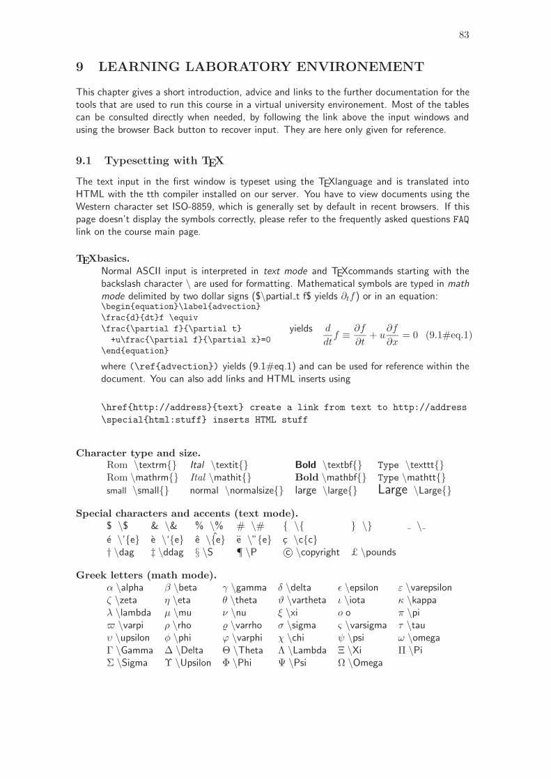
83
9 LEARNING LABORATORY ENVIRONEMENT
This chapter gives a short introduction, advice and links to the further documentation for thetools that are used to run this course in a virtual university environement. Most of the tablescan be consulted directly when needed, by following the link above the input windows andusing the browser Back button to recover input. They are here only given for reference.
9.1 Typesetting with TEX
The text input in the first window is typeset using the TEXlanguage and is translated intoHTML with the tth compiler installed on our server. You have to view documents using theWestern character set ISO-8859, which is generally set by default in recent browsers. If thispage doesn’t display the symbols correctly, please refer to the frequently asked questions FAQlink on the course main page.
TEXbasics.Normal ASCII input is interpreted in text mode and TEXcommands starting with thebackslash character \ are used for formatting. Mathematical symbols are typed in mathmode delimited by two dollar signs ($\partial t f$ yields ∂tf) or in an equation:\beginequation\labeladvection\fracddtf \equiv\frac\partial f\partial t+u\frac\partial f\partial x=0
\endequation
yields d
dtf ≡ ∂f
∂t+ u
∂f
∂x= 0 (9.1#eq.1)
where (\refadvection) yields (9.1#eq.1) and can be used for reference within thedocument. You can also add links and HTML inserts using
\hrefhttp://addresstext create a link from text to http://address\specialhtml:stuff inserts HTML stuff
Character type and size.Rom \textrm Ital \textit Bold \textbf Type \textttRom \mathrm Ital \mathit Bold \mathbf Type \mathttsmall \small normal \normalsize large \large Large \Large
Special characters and accents (text mode).$ \$ & \& % \% # \# \ \ \e \’e e \‘e e \e e \”e c \cc† \dag ‡ \ddag § \S ¶ \P c© \copyright £ \pounds
Greek letters (math mode).α \alpha β \beta γ \gamma δ \delta ε \epsilon ε \varepsilonζ \zeta η \eta θ \theta ϑ \vartheta ι \iota κ \kappaλ \lambda µ \mu ν \nu ξ \xi o o π \pi$ \varpi ρ \rho % \varrho σ \sigma ς \varsigma τ \tauυ \upsilon φ \phi ϕ \varphi χ \chi ψ \psi ω \omegaΓ \Gamma ∆ \Delta Θ \Theta Λ \Lambda Ξ \Xi Π \PiΣ \Sigma Υ \Upsilon Φ \Phi Ψ \Psi Ω \Omega
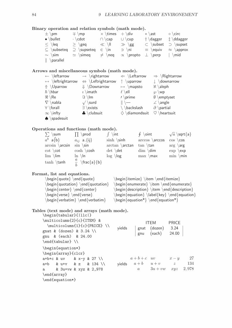
84 9 LEARNING LABORATORY ENVIRONEMENT
Binary operation and relation symbols (math mode).± \pm ∓ \mp × \times ÷ \div ∗ \ast \circ• \bullet · \cdot ∩ \cap ∪ \cup † \dagger ‡ \ddagger≤ \leq ≥ \geq \ll \gg ⊂ \subset ⊃ \supset⊆ \subseteq ⊇ \supseteq ∈ \in 3 \ni ≡ \equiv ≈ \approx∼ \sim ' \simeq 6= \neq ∝ \propto ⊥ \perp | \mid‖ \parallel
Arrows and miscellaneous symbols (math mode).← \leftarrow → \rightarrow ⇐ \Leftarrow ⇒ \Rightarrow↔ \leftrightarrow ⇔ \Leftrightarrow ↑ \uparrow ↓ \downarrow⇑ \Uparrow ⇓ \Downarrow 7→ \mapsto ℵ \aleph~ \hbar ı \imath ` \ell ℘ \wp< \Re = \Im ′ \prime ∅ \emptyset∇ \nabla
√ \surd ‖ \— ∠ \angle∀ \forall ∃ \exists \ \backslash ∂ \partial∞ \infty ♣ \clubsuit ♦ \diamondsuit ♥ \heartsuit♠ \spadesuit
Operations and functions (math mode).∑\sum
∏\prod
∫\int
∮\oint
√a \sqrta
ab ab aij a ij sinh \sinh arccos \arccos cos \cosarcsin \arcsin sin \sin arctan \arctan tan \tan arg \argcot \cot cosh \cosh det \det dim \dim exp \explim \lim ln \ln log \log max \max min \min
tanh \tanha
b\fracab
Format, list and equations.\beginquote \endquote \beginitemize \item \enditemize\beginquotation \endquotation \beginenumerate \item \endenumerate\begincenter \endcenter \begindescription \item \enddescription\beginverse \endverse \beginequation \labelkey \endequation\beginverbatim \endverbatim \beginequation* \endequation*
Tables (text mode) and arrays (math mode).\begintabular|llc|\multicolumn2cITEM &\multicolumn1cPRICE \\
gnat & (dozen) & 3.24 \\gnu & (each) & 24.00\endtabular \\
yieldsITEM PRICE
gnat (dozen) 3.24gnu (each) 24.00
\beginequation*\beginarrayclcra+b+c & uv & x-y & 27 \\a+b & u+v & z & 134 \\a & 3u+vw & xyz & 2,978\endarray\endequation*
yields
a+ b+ c uv x− y 27a+ b u+ v z 134a 3u+ vw xyz 2, 978
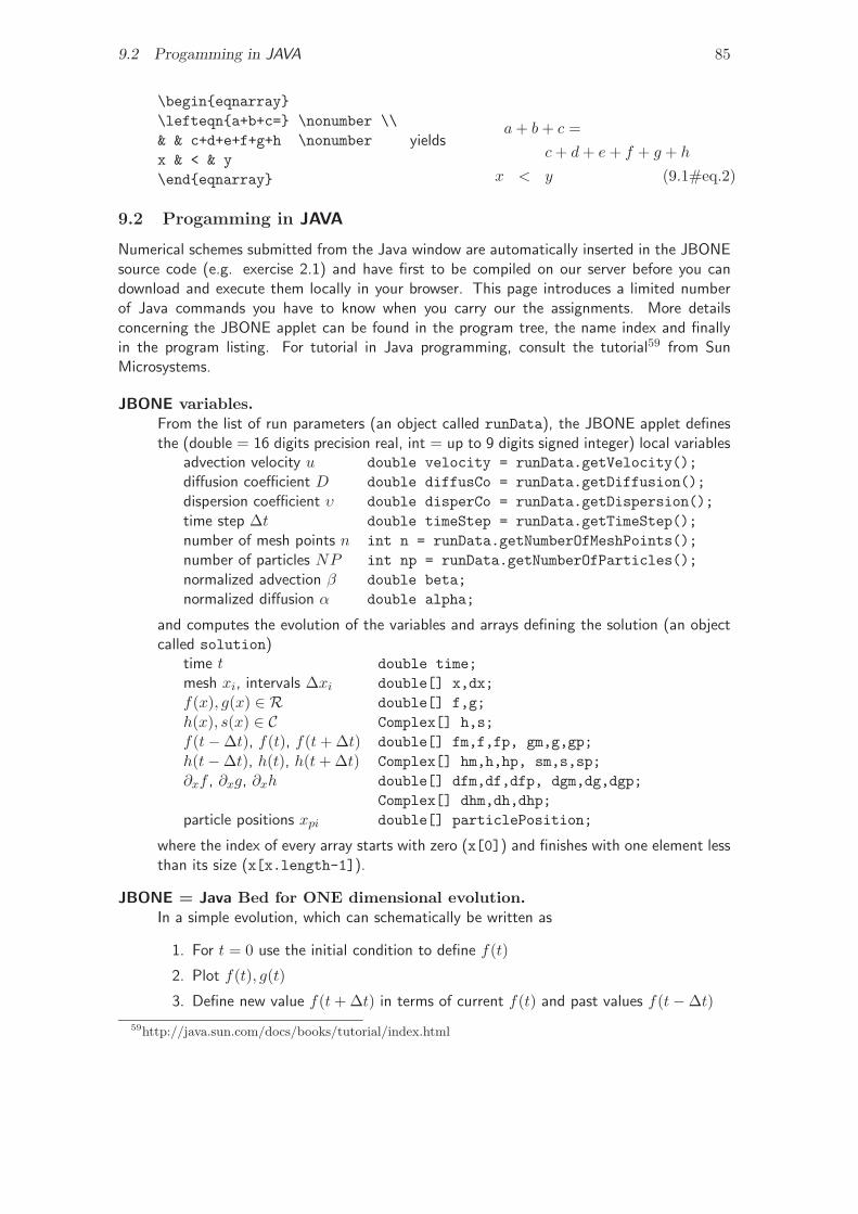
9.2 Progamming in JAVA 85
\begineqnarray\lefteqna+b+c= \nonumber \\& & c+d+e+f+g+h \nonumberx & < & y\endeqnarray
yieldsa+ b+ c =
c+ d+ e+ f + g + h
x < y (9.1#eq.2)
9.2 Progamming in JAVA
Numerical schemes submitted from the Java window are automatically inserted in the JBONEsource code (e.g. exercise 2.1) and have first to be compiled on our server before you candownload and execute them locally in your browser. This page introduces a limited numberof Java commands you have to know when you carry our the assignments. More detailsconcerning the JBONE applet can be found in the program tree, the name index and finallyin the program listing. For tutorial in Java programming, consult the tutorial59 from SunMicrosystems.
JBONE variables.From the list of run parameters (an object called runData), the JBONE applet definesthe (double = 16 digits precision real, int = up to 9 digits signed integer) local variables
advection velocity u double velocity = runData.getVelocity();diffusion coefficient D double diffusCo = runData.getDiffusion();dispersion coefficient υ double disperCo = runData.getDispersion();time step ∆t double timeStep = runData.getTimeStep();number of mesh points n int n = runData.getNumberOfMeshPoints();number of particles NP int np = runData.getNumberOfParticles();normalized advection β double beta;normalized diffusion α double alpha;
and computes the evolution of the variables and arrays defining the solution (an objectcalled solution)
time t double time;mesh xi, intervals ∆xi double[] x,dx;f(x), g(x) ∈ R double[] f,g;h(x), s(x) ∈ C Complex[] h,s;f(t−∆t), f(t), f(t+ ∆t) double[] fm,f,fp, gm,g,gp;h(t−∆t), h(t), h(t+ ∆t) Complex[] hm,h,hp, sm,s,sp;∂xf , ∂xg, ∂xh double[] dfm,df,dfp, dgm,dg,dgp;
Complex[] dhm,dh,dhp;particle positions xpi double[] particlePosition;
where the index of every array starts with zero (x[0]) and finishes with one element lessthan its size (x[x.length-1]).
JBONE = Java Bed for ONE dimensional evolution.In a simple evolution, which can schematically be written as
1. For t = 0 use the initial condition to define f(t)
2. Plot f(t), g(t)
3. Define new value f(t+ ∆t) in terms of current f(t) and past values f(t−∆t)
59http://java.sun.com/docs/books/tutorial/index.html
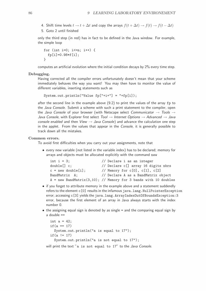
86 9 LEARNING LABORATORY ENVIRONEMENT
4. Shift time levels t→ t+ ∆t and copy the arrays f(t+ ∆t)→ f(t)→ f(t−∆t)5. Goto 2 until finished
only the third step (in red) has in fact to be defined in the Java window. For example,the simple loop
for (int i=0; i<=n; i++) fp[i]=0.98*f[i];
computes an artificial evolution where the initial condition decays by 2% every time step.
Debugging.Having corrected all the compiler errors unfortunately doesn’t mean that your schemeimmediately behaves the way you want! You may then have to monitor the value ofdifferent variables, inserting statements such as
System.out.println("Value fp["+i+"] = "+fp[i]);
after the second line in the example above (9.2) to print the values of the array fp tothe Java Console. Submit a scheme with such a print statement to the compiler, openthe Java Console of your browser (with Netscape select Communicator → Tools →Java Console, with Explorer first select Tool → Internet Options → Advanced → Javaconsole enabled and then View → Java Console) and advance the calculation one stepin the applet. From the values that appear in the Console, it is generally possible totrack down all the mistakes.
Common errors.To avoid first difficulties when you carry out your assignments, note that
• every new variable (not listed in the variable index) has to be declared; memory forarrays and objects must be allocated explicitly with the command new
int i = 3; // Declare i as an integerdouble[] c; // Declare c[] array 16 digits nbrsc = new double[i]; // Memory for c[0], c[1], c[2]BandMatrix A; // Declare A as a BandMatrix objectA = new BandMatrix(3,10); // Memory for 3 bands with 10 doubles
• if you forget to attribute memory in the example above and a statement suddendlyrefers to the element c[0] results in the infamous java.lang.NullPointerExceptionerror; accessing c[3] yields the java.lang.ArrayIndexOutOfBoundsException:3error, because the first element of an array in Java always starts with the indexnumber 0.
• the assigning equal sign is denoted by as single = and the comparing equal sign bya double ==
int a = 42;if(a == 17)System.out.println("a is equal to 17");
if(a != 17)System.out.println("a is not equal to 17");
will print the text ”a is not equal to 17” to the Java Console.
9.3 Parameters and switches in HTML 87
9.3 Parameters and switches in HTML
Editable parameters.The following list of input parameters can be used to change the defaults pre-defined inthe JBONE code:
• Velocity the advection velocity u (or the market interest rate r)
• Diffusion the diffusion D (or the market volatility σ)
• Dispersion the dispersion
• TimeStep the time step ∆t
• MeshPoints the number of mesh points N
• Particles the number of particles Np
• TimeImplicit the time implicit parameter θ
• TuneIntegr the tunable integration parameter p
• ICAmplitude the initial condition amplitude
• ICPosition the initial condition position
• ICWidth the initial condition width
• ICWavelength the initial condition wavelength
• RunTime the physical run time, T=n∆t
• MeshLeft the left position of the mesh x0
• MeshLength the length of the simulation box xN
• PhysDataCase the type of Physical Data, e.g potential shape
• PhysDataValue a Physical Data parameter, e.g potential amplitude
Selectors.The selectors appear over the JBONE plot window and allow you to choose the problemyou want to solve. Careful, white spaces count!
• method selects the numerical method. Choices include”Finite differences”, ”Finite elements”, ”Fourier transform”, ”Monte-Carlo”, ”La-grangian”.
• scheme selects a particular scheme in a given method. Choices include”Standard scheme”, ”Explicit 2-level”, ”Explicit 3-level”, ”Implicit 2-level”, ”Expl-LaxWendroff”, ”Impl-LaxWendroff”, ”Leap-frog (FDTD)”, ”European naive”, ”Eu-ropean vanilla”, ”American vanilla”, ”Tunable Integration”, ”Expanded convol.”,”Aliased convol.”, ”CubicHermite FEM”, ”Cubic – Splines”, ”Forward Euler”,”Forward Euler pp”, ”My scheme”, ”Exercise 2.1”, ”Exercise 2.3”, etc
• ic selects the type of initial condition. Choices include”Box”, ”Gaussian”, ”Cosine”, ”Soliton”, ”WavePacket”, ”PutOption”.
• pde selects the type of PDE. Choices include”Advection”, ”Burger (shock)”, ”KdV (solitons)”, ”Schroedinger”, ”Black-Scholes”,”My equation 1”, ”My equation 2”, ”Exercise”.
TAG defaults.The JBONE applet is included an HTML document with a header of the form
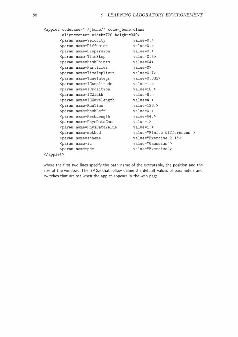
88 9 LEARNING LABORATORY ENVIRONEMENT
<applet codebase="./jbone/" code=jbone.classalign=center width=720 height=340>
<param name=Velocity value=0.><param name=Diffusion value=0.><param name=Dispersion value=0.><param name=TimeStep value=0.5><param name=MeshPoints value=64><param name=Particles value=0><param name=TimeImplicit value=0.7><param name=TuneIntegr value=0.333><param name=ICAmplitude value=1.><param name=ICPosition value=18.><param name=ICWidth value=8.><param name=ICWavelength value=4.><param name=RunTime value=128.><param name=MeshLeft value=0.><param name=MeshLength value=64.><param name=PhysDataCase value=1><param name=PhysDataValue value=1.><param name=method value="Finite differences"><param name=scheme value="Exercise 2.1"><param name=ic value="Gaussian"><param name=pde value="Exercise">
</applet>
where the first two lines specify the path name of the executable, the position and thesize of the window. The TAGS that follow define the default values of parameters andswitches that are set when the applet appears in the web page.
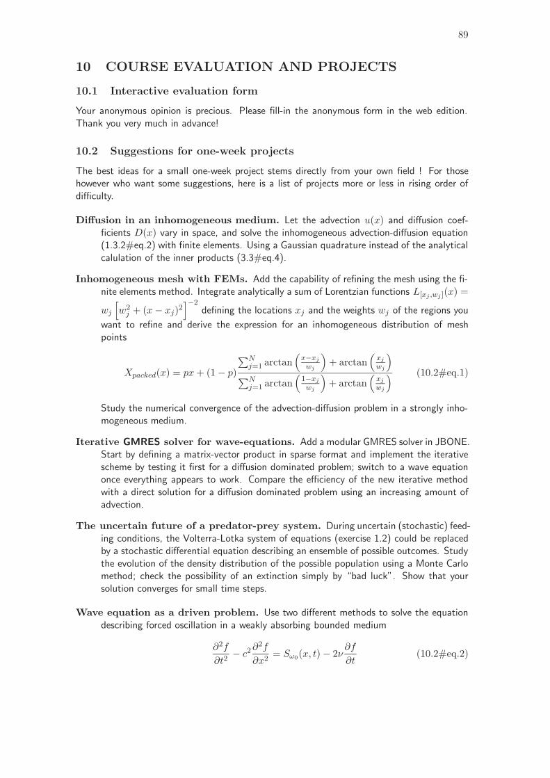
89
10 COURSE EVALUATION AND PROJECTS
10.1 Interactive evaluation form
Your anonymous opinion is precious. Please fill-in the anonymous form in the web edition.Thank you very much in advance!
10.2 Suggestions for one-week projects
The best ideas for a small one-week project stems directly from your own field ! For thosehowever who want some suggestions, here is a list of projects more or less in rising order ofdifficulty.
Diffusion in an inhomogeneous medium. Let the advection u(x) and diffusion coef-ficients D(x) vary in space, and solve the inhomogeneous advection-diffusion equation(1.3.2#eq.2) with finite elements. Using a Gaussian quadrature instead of the analyticalcalulation of the inner products (3.3#eq.4).
Inhomogeneous mesh with FEMs. Add the capability of refining the mesh using the fi-nite elements method. Integrate analytically a sum of Lorentzian functions L[xj ,wj ](x) =
wj
[w2j + (x− xj)2
]−2defining the locations xj and the weights wj of the regions you
want to refine and derive the expression for an inhomogeneous distribution of meshpoints
Xpacked(x) = px+ (1− p)∑N
j=1 arctan(x−xjwj
)+ arctan
(xjwj
)∑N
j=1 arctan(
1−xjwj
)+ arctan
(xjwj
) (10.2#eq.1)
Study the numerical convergence of the advection-diffusion problem in a strongly inho-mogeneous medium.
Iterative GMRES solver for wave-equations. Add a modular GMRES solver in JBONE.Start by defining a matrix-vector product in sparse format and implement the iterativescheme by testing it first for a diffusion dominated problem; switch to a wave equationonce everything appears to work. Compare the efficiency of the new iterative methodwith a direct solution for a diffusion dominated problem using an increasing amount ofadvection.
The uncertain future of a predator-prey system. During uncertain (stochastic) feed-ing conditions, the Volterra-Lotka system of equations (exercise 1.2) could be replacedby a stochastic differential equation describing an ensemble of possible outcomes. Studythe evolution of the density distribution of the possible population using a Monte Carlomethod; check the possibility of an extinction simply by “bad luck”. Show that yoursolution converges for small time steps.
Wave equation as a driven problem. Use two different methods to solve the equationdescribing forced oscillation in a weakly absorbing bounded medium
∂2f
∂t2− c2∂
2f
∂x2= Sω0(x, t)− 2ν
∂f
∂t(10.2#eq.2)
90 10 COURSE EVALUATION AND PROJECTS
Choose a source Sω0(x, t) = S0 exp(x2/∆2) sin(ω0t) smoothly distributed inside thecavity x ∈ [−L/2;L/2] and a sink ν ω0 ' 2πc/L which is sufficiently small to allowthe perturbations to propagate and reflect. Vary the driving frequency ω0 and study thepossibility of exciting resonances inside the cavity.
Particle weight. Apply individual weights wi to the particles in the Monte Carlo solver. Tryto reduce the amount of noise at low levels in a steady state solution (e.g. exercise 5.4)by splitting particles with wi > wlimit(x). Try to find a good maximum weight func-tion wlimit(x). After a while some particles will be to heavy. Solve this by re-discretizingthe distribution function with a call to discretize(new ShapeNumerical(this));The particle weight should be used to increase the accuracy in discretization. Thisproject involves changing the projection, the discretization and learning the Vectorclass in Java.
Option pricing. Study the finite difference schemes proposed for the price of a Europeanput option in financial and lognormal variables (exercise 2.5) and implement the implicitfinite element scheme for an American put (exercise 3.5) in financial variables. Completethe project by implementing a Monte-Carlo solver along the same lines.
Bose-Einstein condensation. Start with the linear Schrodinger equation
i∂ψ
∂t=[− ∂2
∂x2+ V (x)
]ψ (10.2#eq.3)
normalized with Plank’s constant ~ = 1 and a particle mass m = 1/2 and use two differ-ent schemes to calculate the scattering of a wavepacket by a simple one-dimensional po-tential V (x). Having validated your schemes with analytical results, solve the non-linearequation describing the Bose-Einstein condensation in a parabolic trapping potentialV (r) = α
2 r2 with cylindrical symmetry
i∂ψ
∂t=[−1r
∂
∂r
(r∂
∂r
)+ V (r) + 2πa | ψ |2
]ψ (10.2#eq.4)
where the parameter a defines the scattering length.
Slowing down of beams. The slowing down of a beam in a collisional media is given by
∂f(x, v, t)∂t
+ v∂f(x, v, t)
∂x+
∂
∂v[−vpvf(x, v, t)] =
∂
∂v
(Dp
∂f(x, v, t)∂v
)(10.2#eq.5)
Use Monte Carlo for solving the beam distribution function. Identify the drift anddiffusion coefficients in x and v. Start the pulse to the left with v = v0. Modify vpand Dp in order to get a nice slowing down of the pulse.
KdV with wavelets.
REFERENCES 91
References
[1] J. P. Berenger. A perfectly matched layer for the absorption of electomagnetic waves.Journal of Computational Physics, 114:185, 1994.
[2] M. Abramowitz and A. Stegun. Handbook of Mathematical Functions. Dover Publica-tions, New York, tenth edition, 1972.
[3] W. Sweldens. The Wavelet Home Page60.
[4] W. H. Press, S. A. Teukolsky, W. T. Vetterling, and B. P. Flannery. Numerical Recipies61.Cambridge University Press, second edition, 1992.
[5] J. M. Sanz-Serna and P. Calvao. Numerical Hamiltonian Problems. Chapman & Hall,1994.
[6] G. Dahlquist and A Bjorck. Numerical Methods. Prentice-Hall, 1974.
[7] C. A. Fletcher. Computational Techniques for Fluid Dynamics. Springer, second edition,1991.
[8] C. Johnson. Numerical Solution of PDEs by the FEM Method. Studentlitteratur – Lund,Sweden, 1987.
[9] K. Appert. Experimentation numerique. unpublished lecture notes, CRPP-EPFL, CH-1015 Lausanne, Switzerland, 1988.
[10] National Institute of Standards and Technology (NIST). Guide to Available MathematicalSoftware62.
[11] J. Eastwood. Computer Physics Communications Library63.
[12] I. M.Ryzhik I. S. Gradshteyn. Table of integrals, series and products. Academic Press,New York, 1980.
[13] N.W. Ashcroft and N.D. Mermin. Solid State Physics. Holt-Saunders InternationalEditions, 1976.
[14] J. Boris. Methods in Computational Physics, Vol.16. Academic, 1976.
[15] J. M. Jin. The Finite Element Method in Electromagnetics. John Wiley, 1993.
[16] D. Katz and T. Cwik. EMLIB homepage64.
[17] Y. Saad. Iterative Methods for Sparse Linear Systems. PWS Publishing Company, 1996.
[18] P. Wilmott, J. Dewynne, and S. Howison. Option Pricing. Oxford Financial Press, 1993.
[19] T. Bjork. Examples in optimization theory. unpublished lecture notes, Inst. for Optimiza-tion and System Theory, KTH, SE-100 44 Stockholm, Sweden, 1995.
60http://www.wavelet.org/wavelet/index.html61http://www.ulib.org/webRoot/Books/Numerical Recipes/bookcpdf.html62http://gams.nist.gov63http://www.cpc.cs.qub.ac.uk/cpc/64http://http://emlib.jpl.nasa.gov/
92 REFERENCES
[20] D. Duffie. Dynamic Asset Pricing Theory. Princeton University Press, 1992.
[21] R. Rebonato. Interest-Rate Option Models. Wiley & Sons Ldt, UK, 1996.
[22] A. Bondeson and G. Y. Fu. Tunable integration scheme. Computer Physics Communi-cations, 66:167, 1991.
[23] S. Betts, S. Browne, J. Dongarra, E. Grosse, P McMahan, and T. Rowan. Netlib SoftwareRepository65.
[24] S. Balay, W. D. Gropp, L. C. McInnes, and B. F. Smith. PETSc home page. The PETSchome page66, 1999.
[25] A. Jaun, K. Blomqvist, A. Bondeson, and T. Rylander. Iterative solution of global elec-tromagnetic wavefields with finite elements. Computer Physics Communications, 2001.
[26] P. E. Kloeden and E. Platen. Numerical Solution of Stochastic Differential Equations.Springer-Verlag, second corrected printing edition, 1995.
[27] N.G. Van Kampen. Stochastic Processes in Physics and Chemistry. North-Holland Per-sonal Library, 1992.
[28] J. Carlsson. The Monte-Carlo method – a cookbook approach67. Alfven Laboratory,KTH, SE-100 44 Stockholm, Sweden, 1997.
[29] C. K. Birdsall and A. B. Langdon. Plasma physics via computer simulation. McGraw-Hill,1985. The Plasma Theory and Simulation Group Homepage68.
[30] R. W. Hockney and J. W. Eastwood. Computer Simulation Using Particles. Adam Hilger,1988.
[31] T. Yabe and T. Aoki. A universal solver for hyberbolic equations by cip. ComputerPhysics Communications, 66:219, 1991.
[32] H. Takewaki and T. Yabe. The cubic-interpolated pseudo particle (cip) method. ComputerPhysics Communications, 70:355, 1987.
[33] T. Utsumi, T. Kunugi, and T. Aoki. Stability and accuracy of the cip scheme. ComputerPhysics Communications, 101:9, 1997.
65http://www.netlib.org66http://www.mcs.anl.gov/petsc67http://fedu52.fed.ornl.gov/%7ecarlsson/MonteCarlo/cookbook/notes.html68http://ptsg.eecs.berkeley.edu/
Related Documents